the fractal structure of cellular automata on abelian groups
TRANSCRIPT
HAL Id: hal-01185495https://hal.inria.fr/hal-01185495
Submitted on 20 Aug 2015
HAL is a multi-disciplinary open accessarchive for the deposit and dissemination of sci-entific research documents, whether they are pub-lished or not. The documents may come fromteaching and research institutions in France orabroad, or from public or private research centers.
L’archive ouverte pluridisciplinaire HAL, estdestinée au dépôt et à la diffusion de documentsscientifiques de niveau recherche, publiés ou non,émanant des établissements d’enseignement et derecherche français ou étrangers, des laboratoirespublics ou privés.
The fractal structure of cellular automata on abeliangroups
Johannes Gütschow, Vincent Nesme, Reinhard F. Werner
To cite this version:Johannes Gütschow, Vincent Nesme, Reinhard F. Werner. The fractal structure of cellular automataon abelian groups. Automata 2010 - 16th Intl. Workshop on CA and DCS, 2010, Nancy, France.pp.51-70. �hal-01185495�
Automata 2010 — 16th Intl. Workshop on CA and DCS DMTCS proc. AL, 2010, 51–70
The fractal structure of cellular automata onabelian groups
Johannes Gutschow, Vincent Nesme, and Reinhard F. WernerInstitut fur Theoretische Physik, Universitat Hannover, Hannover, Germany
It is a well-known fact that the spacetime diagrams of some cellular automata have a fractal structure: forinstance Pascal’s triangle modulo 2 generates a Sierpinski triangle. Explaining the fractal structure of thespacetime diagrams of cellular automata is a much explored topic, but virtually all of the results revolvearound a special class of automata, whose main features include irreversibility, an alphabet with a ringstructure and a rule respecting this structure, and a property known as being (weakly) p-Fermat. The classof automata that we study in this article fulfills none of these properties. Their cell structure is weaker andthey are far from being p-Fermat, even weakly. However, they do produce fractal spacetime diagrams, andwe will explain why and how.
These automata emerge naturally from the field of quantum cellular automata, as they include the classicalequivalent of the Clifford quantum cellular automata, which have been studied by the quantum commu-nity for several reasons. They are a basic building block of a universal model of quantum computation, andthey can be used to generate highly entangled states, which are a primary resource for measurement-basedmodels of quantum computing.
Keywords: fractal, abelian group, linear cellular automaton, substitution system
IntroductionThe fractal structure of cellular automata (CA) has been a topic of interest for several decades.In many works on linear CA, the authors present ways to calculate the fractal dimension or topredict the state of an arbitrary cell at an arbitrary time step, with much lower complexity thanby running the CA step by step; however, their notions of linearity are quite different. Oftenonly CA that use states in Zp
(i) are studied; other approaches are more general, but still makecertain assumptions on the time evolution or the underlying structure of the CA. In this workwe try to loosen these restrictions as far as possible. We consider one-dimensional linear CAwhose alphabet is an abelian group. We show how they can be described by n× n matrices withpolynomial entries and use this description to derive a recursion relation for the iterations of theCA. This recursion relation enables us to formulate the evolution of the spacetime diagram as a
(i) We use the simple notation Zd for the cyclic group of order d, instead of Z/dZ, as we are concerned with finite groupsonly.
1365–8050 c© 2010 Discrete Mathematics and Theoretical Computer Science (DMTCS), Nancy, France
52 Johannes Gutschow, Vincent Nesme, and Reinhard F. Werner
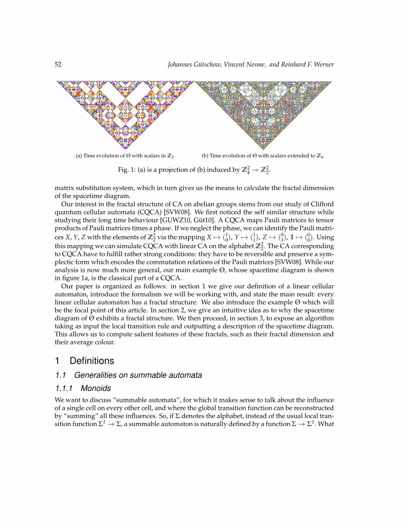
(a) Time evolution of Θ with scalars in Z2. (b) Time evolution of Θ with scalars extended to Z4.
Fig. 1: (a) is a projection of (b) induced by Z24 � Z2
2.
matrix substitution system, which in turn gives us the means to calculate the fractal dimensionof the spacetime diagram.
Our interest in the fractal structure of CA on abelian groups stems from our study of Cliffordquantum cellular automata (CQCA) [SVW08]. We first noticed the self similar structure whilestudying their long time behaviour [GUWZ10, Gut10]. A CQCA maps Pauli matrices to tensorproducts of Pauli matrices times a phase. If we neglect the phase, we can identify the Pauli matri-ces X, Y, Z with the elements of Z2
2 via the mapping X 7→ (10), Y 7→ (1
1), Z 7→ (01), 1 7→ (0
0). Usingthis mapping we can simulate CQCA with linear CA on the alphabet Z2
2. The CA correspondingto CQCA have to fulfill rather strong conditions: they have to be reversible and preserve a sym-plectic form which encodes the commutation relations of the Pauli matrices [SVW08]. While ouranalysis is now much more general, our main example Θ, whose spacetime diagram is shownin figure 1a, is the classical part of a CQCA.
Our paper is organized as follows: in section 1 we give our definition of a linear cellularautomaton, introduce the formalism we will be working with, and state the main result: everylinear cellular automaton has a fractal structure. We also introduce the example Θ which willbe the focal point of this article. In section 2, we give an intuitive idea as to why the spacetimediagram of Θ exhibits a fractal structure. We then proceed, in section 3, to expose an algorithmtaking as input the local transition rule and outputting a description of the spacetime diagram.This allows us to compute salient features of these fractals, such as their fractal dimension andtheir average colour.
1 Definitions1.1 Generalities on summable automata
1.1.1 MonoidsWe want to discuss “summable automata”, for which it makes sense to talk about the influenceof a single cell on every other cell, and where the global transition function can be reconstructedby “summing” all these influences. So, if Σ denotes the alphabet, instead of the usual local tran-sition function ΣI → Σ, a summable automaton is naturally defined by a function Σ→ ΣI . What
The fractal structure of cellular automata on abelian groups 53
is then the minimal structure on Σ that would make such a definition work? These influenceshave to be “summed”, so we need an operation on Σ. Since the strip is infinite, an infinitaryoperation would do, but that wouldn’t give us much to work with. Instead, it seems reasonableto consider a binary operation +. In the same spirit, when we think of the superposition ofinfluences coming from each cell, no notion of order between the cells is involved; even if in theone-dimensional case a natural order can be put on the cells, it would be less than clear what todo in higher dimensions. We require therefore that + be associative and commutative. The lastrequirement comes from the fact that, given only the global transition function, we want to beable to isolate the influence of one cell; that is why we demand that + have an identity element,which makes now (Σ,+) an abelian monoid. Of course, in order for all of this to be relevant, thetransition function has to be a morphism.
Let I be some finite subset of Z and f a morphism from Σ to ΣI . From f one can define theglobal transition function as an endomorphism F of ΣZ by
F :
ΣZ → ΣZ
r = (rn)n∈Z 7→(
∑i∈I
f (rn−i)i
)n∈Z
. (1)
Let σ be the right shift on ΣZ, i.e. σ(r)n = rn−1. We have F ◦ σ = σ ◦ F, which means F istranslation invariant. Also, F(r)n depends only on the values rn−i for i ∈ I; since I is finite, F isa one-dimensional cellular automaton on the alphabet Σ, with neighbourhood included in −I.Conversely, if F is an endomorphism of ΣZ defining a cellular automaton over the alphabet Σ,then one can choose a neighbourhood I, and define, for i ∈ I,
f (s)i = F(s)i, (2)
where s is the word of ΣZ defined by sn =
{s if n = 0e otherwise , e denoting the neutral element of
Σ.
1.1.2 GroupsWe will now consider the case when Σ is a (finite abelian) group. For p prime, let Σp be thesubgroup of Σ of elements of order a power of p; then Σ is isomorphic to ∏
pΣp, and every
endomorphism of ΣZ factorises into a product of endomorphisms of the ΣZp ’s. It is therefore
enough to study the case of the (abelian) p-groups: let us assume Σ is a p-group.It is a well-known fact (see for instance section I-8 of [Lan93]) that Σ is isomorphic to Zpk1 ×
Zpk2 × · · · ×Zpkd with kd ≥ kd−1 ≥ . . . ≥ k1 = k. Consider an endomorphism α of Σ andlet ej denote (0, . . . , 0, 1, 0, . . . , 0), where the 1 lies in position j. When i ≥ j, there is a naturalembedding si,j of Zpki into Z
pkj , namely the multiplication by pkj−ki ∈ N. Since ej has order
pkj , α(ej)i ∈ Zpki has to be in the image of sj,i when i ≤ j. We can therefore associate to α the
endomorphism of Zdpk given by the matrix A(α) ∈Md(Zpk ) defined by A(α)i,j = pkj−ki α
(ej)
i.

54 Johannes Gutschow, Vincent Nesme, and Reinhard F. Werner
For instance, if G is Z32 × Z4 × Z2, and α is defined by α(1, 0, 0) = (3, 2, 1), α(0, 1, 0) =(24, 0, 1) and α(0, 0, 1) = (16, 2, 0), then the corresponding matrix of M3 (Z32) would be
A(α) =
3 3 116 0 116 2 0
.
Let us give a summary of the construction we have just exposed.
Proposition 1 For every finite abelian p-group G and endomorphism α of G, there are positive integers kand d, an embedding s of G into Zd
pk , and an endomorphism A(α) of Zdpk such that the following diagram
commutes:
G α−−−−→ Gysys
Zdpk
A(α)−−−−→ Zdpk
(3)
This implies that to study the behaviour of CA on abelian groups, it is enough to study thecase where these groups are of the form Zd
pk .
1.1.3 R-modulesWe will actually consider the more general case where R is a finite commutative ring, and Σ is afree R-module of dimension d, i.e. isomorphic to Rd. The first reason for doing so is that it doesnot complicate the mathematics. It will also appear more efficient to understand, for instance,F24 as a 1-dimensional vector space over itself than as a 4-dimensional vector space over F2: theformer simply bears more information, and therefore implies more restrictions on the form of aCA, so that more can be deduced.
For any ring B, B[u, u−1] denotes the ring of Laurent polynomials over B; it is the ring of
linear combinations of integer powers (negative as well as nonnegative) of the unknown u.Applying this to B = HomR (Σ), we can associate to the function f the Laurent polynomialτ( f ) ∈ HomR (Σ)
[u, u−1] defined by
τ( f ) = ∑n∈Z
f (·)nun. (4)
τ is an isomorphism of R-algebras between the linear cellular automata on the alphabet Σwith internal composition rules (+, ◦) and HomR (Σ)
[u, u−1], which can be identified with
Md(
R[u, u−1]) because Σ ' Rd; we are going to think and work in this former algebra, so from
now on a linear cellular automaton T = τ( f ) will be for us an element of Md(
R[u, u−1]).
1.2 Related workMany papers have been published about the fractal structure of cellular automata spacetimediagrams. We give here a short review and point out the differences to our approach. When wemention d and k we are referring to Md
(Zk[u, u−1]
).

The fractal structure of cellular automata on abelian groups 55
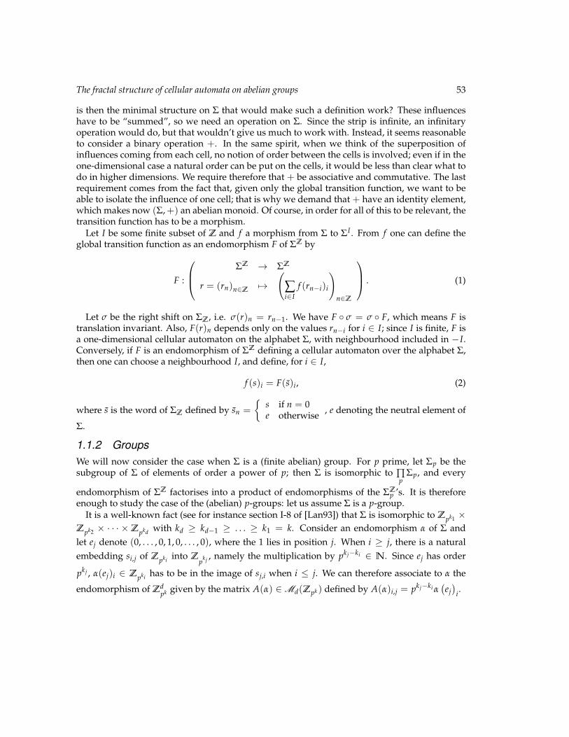
(a) Time evolution of Θ starting from ξ = (10).
3p
2p
p
(b) Time evolution of a general nearest neighbour p-FermatCA.
Fig. 2: This figure shows that Θ cannot be a p-Fermat CA. In a p-Fermat CA at least the whiteareas are filled by the neutral element e; Θ has a different pattern.
[Wil87] In this work, Willson considers the case d = 1, k = 2. In order to determine the fractaldimension of the spacetime diagram, he analyses how blocks of length n in the configura-tion of time step t are mapped to such blocks in steps 2t and 2t + 1, a technique we alsouse in section 3.
[Tak90, Tak92] Takahashi generalises Willson’s work to the case d = 1, with no restriction onthe value of k.
[HPS93, HPS01] Haeseler et al. study the fractal time evolution of CA with special scaling prop-erties, the weakest of them being “weakly p-Fermat”, where p is some integer, which in-cludes the case d = 1, k = p. Let us briefly introduce the p-Fermat property and showwhy the CA studied by us do not have to be p-Fermat. Let πp be the scaling map
πp(ξ)x =
{ξy if x = pye otherwise . (5)
A CA T is weakly p-Fermat if for all s ∈ Σ, n ∈N and x ∈ Z, Tnp(s)x = e⇔ πpTn(s)x = e.
Let us now consider
Θ =
(0 11 u−1 + 1 + u
)∈M2(Z2[u, u−1]). (6)
We will use this example throughout the paper. It generates the time evolution depictedin Figure 2a. A general nearest-neighbour p-Fermat CA produces a time evolution thatreproduces itself after p steps in at most three copies located at positions {−p; 0; p}. After2p steps we have five copies at most. This creates areas filled with the neutral element eshared by all p-Fermat CA for a fixed p. In figures 2a and 2b we can easily see that Θ doesnot exhibit these areas. Thus it is not p-Fermat. Furthermore p-Fermat CA that are notperiodic are irreversible, while we also allow reversible CA, Θ being again one example.
56 Johannes Gutschow, Vincent Nesme, and Reinhard F. Werner
[AHPS96, AHP+97] Allouche et al. study recurrences in the spacetime diagram of linear cellu-lar automata, from the angle of k-automatic sequences, which we will not define in thispaper. However they require Σ to be an abelian ring and the CA to be a ring homomor-phism, which is again essentially the case d = 1.
[Moo97, Moo98] Moore studies CA with an alphabet A on a staggered spacetime, where everycell c is only influenced by two cells a and b of the last time step. The update rule isc = a • b. He requires (A, •) to be a quasigroup and studies different special cases. Firstlet us note that these CA are irreversible, while ours don’t have to be. Thus, although itis possible to bring our CA in the form of a staggered CA, the results of Moore do notapply. In his setting, our CA would be of the form c = a • b = f (a) + g(b) for somehomomorphisms f and g. For (A, •) to be a quasigroup means
∀a, b ∈ A ∃!x, y ∈ A a • x = b ∧ y • x = b. (7)
In our case, the required equalities translate respectively as g(x) = b− f (a) and f (y) =b− g(a). The right-hand sides are each arbitrary elements of A, thus f and g have to beisomorphisms, as indeed required in [Moo97].
The angle of study of Moore is also different: he does not exactly study fractal propertiesof the CA, but rather the complexity of the prediction — “What will be the state of this cellafter t steps?”. Describing the spacetime diagram with a matrix substitution system is analternative way of proving that prediction is an easy task — for instance it makes it NC.
[Mac04] Macfarlane uses Willson’s approach and generalises parts of it to matrix-valued CA,his examples including Θ. However, the transition matrix is obtained heuristically — “byscrutiny of figure 9” — from the spacetime diagram, instead of being algorithmically de-rived from the transition rule (as in the present work). The conclusion (section 6) suggeststhat the analysis of Θ is easily generalisable to matrices of various sizes over various rings,so in a sense the present article is but an elaboration of the concluding remark of [Mac04],although we have to say we do not find this generalisation to be that obvious.
The heart of the proof is in section 3. In a nutshell, whereas most of the techniques used in ourarticle can be traced back to older articles, the new one that allows us to extend the analysis to alarger class of automata is the introduction of α in equation (20). The idea in doing so is to getrid of the complicated noncommutative ring structure and go back to a simple linear recurrence,as state in Proposition 4. Since a linear recurrence is precisely where the analysis started from,it could seem at first sight that nothing is gained in the process, but the new recurrence actuallydoes not define a cellular automaton. Instead of defining line n + 1 from line n, it cuts rightthrough to line mn, thus establishing a scaling property.
1.3 Different CAWhile we use Θ, which has very special properties (being reversible, over a field of characteristictwo, and described by a 2× 2 matrix) as our example throughout the paper, the analysis appliesof course to all other linear CA. In this section we give a short overview over the variety of
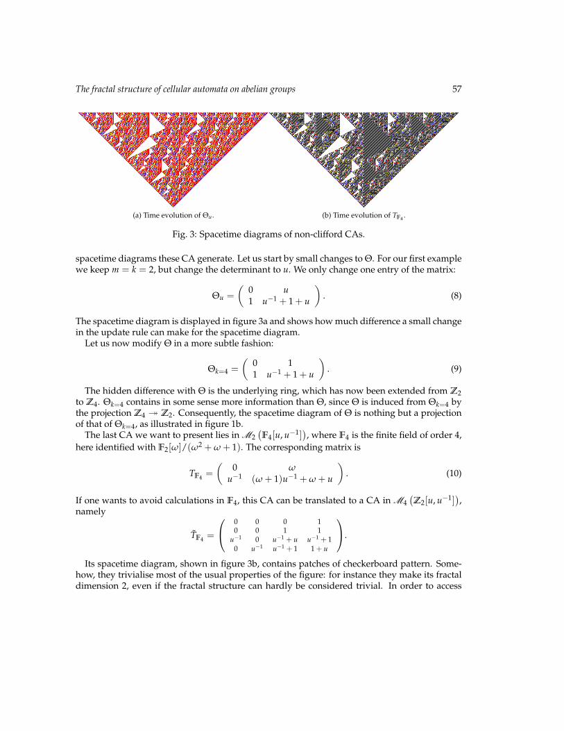
The fractal structure of cellular automata on abelian groups 57
(a) Time evolution of Θu. (b) Time evolution of TF4 .
Fig. 3: Spacetime diagrams of non-clifford CAs.
spacetime diagrams these CA generate. Let us start by small changes to Θ. For our first examplewe keep m = k = 2, but change the determinant to u. We only change one entry of the matrix:
Θu =
(0 u1 u−1 + 1 + u
). (8)
The spacetime diagram is displayed in figure 3a and shows how much difference a small changein the update rule can make for the spacetime diagram.
Let us now modify Θ in a more subtle fashion:
Θk=4 =
(0 11 u−1 + 1 + u
). (9)
The hidden difference with Θ is the underlying ring, which has now been extended from Z2to Z4. Θk=4 contains in some sense more information than Θ, since Θ is induced from Θk=4 bythe projection Z4 � Z2. Consequently, the spacetime diagram of Θ is nothing but a projectionof that of Θk=4, as illustrated in figure 1b.
The last CA we want to present lies in M2(F4[u, u−1]
), where F4 is the finite field of order 4,
here identified with F2[ω]/(ω2 + ω + 1). The corresponding matrix is
TF4 =
(0 ω
u−1 (ω + 1)u−1 + ω + u
). (10)
If one wants to avoid calculations in F4, this CA can be translated to a CA in M4(Z2[u, u−1]
),
namely
TF4 =
0 0 0 10 0 1 1
u−1 0 u−1 + u u−1 + 10 u−1 u−1 + 1 1 + u
.
Its spacetime diagram, shown in figure 3b, contains patches of checkerboard pattern. Some-how, they trivialise most of the usual properties of the figure: for instance they make its fractaldimension 2, even if the fractal structure can hardly be considered trivial. In order to access
58 Johannes Gutschow, Vincent Nesme, and Reinhard F. Werner
more interesting properties, it is possible to blank this pattern out, considering it as just “anothershade of white”. This can be trivially done on the matrix substitution system, by removing thestates from which the blank state is inaccessible.
1.4 Coloured spacetime diagramsThe mainstream setting when studying the fractal structure of spacetime diagrams is monochro-matic; we introduce colours in the picture.
Instead of considering simple compact subsets of the plane, we will have a finite set of coloursC and compact subsets of
(R2)C . Let b 6∈ C be the additional “blank” colour and c : Σ →
C ∪ {b} a colouring of Σ such that c(0) = b. To determine a coloured spacetime diagram, weneed furthermore to be given an automaton T ∈Md
(R[u, u−1]), an initial state ξ ∈ Rd, and an
integer n. The corresponding coloured spacetime diagram is then the rescaled diagram obtainedby iteratively applying T n times on ξ.
Formally, for n, i, j ∈N, let Sn,i,j be the full square centred in 1n (i, j) and whose edges, parallel
to the axes, are of length 1n . To each positive integer n and colour c ∈ C is associated a compact
subset of the plane Pn(c) which is the union of the Sn,i,j’s such that 0 ≤ j ≤ n and c(T j (ξ)i
)= c.
The coloured spacetime diagram of order n is then the function Pn : c 7→Pn(c). A sequence ofcoloured patterns (Pn)n∈N of spacetime diagrams is said to converge to some coloured patternP∞ if for every c ∈ C , (Pn(c))n∈N converges to P∞(c) for the Hausdorff distance.
We can now state our main result.
Theorem 1 Let G be a finite abelian p-group. For every cellular automaton over G that is also a grouphomomorphism, there exists a positive integer m such that for every fixed initial state the coloured space-time diagrams of order pmn converge when n goes to infinity.
In general, to know about the fractal structure of a cellular automaton over some finite groupG, write G as a product of p-groups and study each p-component of the spacetime diagram in-dependently; according to Theorem 1, each component generates a fractal pattern. Then, sincethe logarithms of the prime numbers are rationally independent, it is possible to find a sequenceof resized spacetime diagrams that converges towards a superposition of these different com-ponents with arbitrary independent rescaling coefficients, but there is no direct generalisationof the theorem. For instance, even in the simple case of Pascal’s triangle modulo 6, there is noreal number α > 0 such that the diagrams of order bαnc converge; however those of order tnwill converge as soon as the fractional parts of log3(tn) and log2(tn) both converge, and thentheir limits determine the limit pattern. The situation is described very briefly in the section 5 of[Tak92].
1.4.1 Matrix substitution systemsWe will show how to find a suitable description of the limit pattern in the rest of this article. Wenow explain exactly what it means to generate a coloured picture by rules of substitution, andhow to take the limit of all these pictures. This is a generalisation of the usual monochromaticdescription that can be found for instance in [MGAP85, Wil87, HPS93], and which correspondsin our setting to the case where all the colours are mapped to “black”.
The fractal structure of cellular automata on abelian groups 59
Let V be a finite alphabet; because we want colours, compared with the usual definition ofa matrix substitution system, we don’t have to include a special ”empty” letter. A matrix sub-stitution system is then a function D : V → VJ1;rK2
; for some integer r. Together with a setof colours C and a colouring c : V → C , it defines coloured patterns, much in the same waycellular automata do. With the previous notations, at each step n, the pattern Pn is the union ofsquares Srn ,i,j of different colours, for different i’s and j’s; each one of them is indexed by someletter in V.
Then at step n + 1, each coloured square of colour c indexed by v ∈ V present in the nth steppattern is replaced by r2 smaller squares that pave it; these smaller squares are given by D(v)and indexed accordingly. To such a matrix substitution system we can associate a multigraphΓ = (V, E) where the set of vertices is V and we put as many edges from v to w as there are w’sin D(v).
A plain matrix substitution system is one of the usual kind: no colouring, and V contains aspecial letter ε such that D (ε) is a matrix full of ε’s and c(ε) = b. In the multigraph associated toa plain matrix substitution system, ε is excluded from the set of vertices.
We want to generalise the usually property of convergence of the patterns defined by plainmatrix substitution systems. This will be done by the conjunction of the two following proposi-tions. Let us first remind some notions on graphs: the period of a graph is the greatest commondivisor of the lengths of all the cycles in Γ; a graph is aperiodic if it has period 1.
Proposition 2 If every strongly connected component of Γ is aperiodic, then (Pn)n∈N converges.
Proof: To each colour c ∈ C we associate the plain matrix substitution system D c, obtained fromD simply by turning some letters into ε. For v ∈ V, let Xc(v) be the set of integers n such thatthere exists a path of length n in Γ connecting v to a letter of the colour c. Since the stronglyconnected component containing v is aperiodic, Xc(v) is either finite or cofinite. Those lettersv ∈ V such that Xc(v) is finite are sent to ε, and this defines D c. If Xc(v) is finite and v′ can bereached from v, then Xc(v′) is also finite; therefore, D c is indeed a substitution system. Let M besuch that for every v ∈ V, either Xc(v) or its complement is strictly bounded by M.
Let us now compare two sequences of figures. The first one is (Pn(c)), the subpattern ofcolour c defined by D . The second one is (Pc
n), the one obtained from D c; we know that itconverges to some compact D c
∞. By construction, Pn+M(c) is included in Pcn, and for every
black square of Pcn, there is a black subsquare in Pn+M(c). The Hausdorff distance between
Pn+M(c) and Pcn therefore converges to 0, so that (Pn(c)) converges to D c
∞. 2
For a graph Γ, let Γk = (V, Ek) be defined by
(v0, vk) ∈ Ek ⇐⇒ (∃v1, . . . , vk−1 ∈ V ∀i ∈ {0, . . . , k− 1} (vi, vi+1) ∈ E) . (11)
Proposition 3 For every (multi)graph Γ, there exists k such that every strongly connected component ofΓk is aperiodic.
Proof: Each strongly connected component ∆ of Γ has a period p(∆), so that ∆p(∆) is aperiodic.Let k0 be the least common divisor of the p(∆)’s; then each strongly connected component ofΓ induces an aperiodic graph in Γk0 , but it is possible that, in the process, it broke down into

60 Johannes Gutschow, Vincent Nesme, and Reinhard F. Werner
several connected components, so that Γk0 might not have the required property. The procedurethen has to be repeated from Γk0 to obtain Γk0k1 , and so on. Since the strongly connected com-ponents of Γk0···ki+1 are included in those of Γk0···ki , this process reaches a fixed point, which is agraph with the required property. 2
Ergo, a coloured matrix substitution system defines a convergent coloured pattern when con-sidering the steps that are a multiple of some well-chosen integer m. So, in order to proveTheorem 1, all we need to do is find such a substitution system. This will be done in a specialcase in the next section, and in the general case in section 3.
2 A special recursion scheme for ΘThe aim of this section is to give the most direct and natural explanation of the fractal structuregenerated by Θ that we are aware of. Modulo some caveat, it applies effortlessly to all invertibleelements T of M2
(R[u, u−1]
), where R is a finite abelian ring of characteristic 2. This section
is not vital to the proof of the general case presented in 3, and can therefore be skipped by theimpatient reader.
We will deduce informally the basic structure of the spacetime diagrams from a simple re-cursion relation for the 2n-th powers of T. The characteristic polynomial of T, PT(X), is equalto X2 + (tr T) + det T. According to Cayley-Hamilton theorem, PT(T) = 0, so T2 + (tr T) T +(det T) I = 0. Multiplying this equation by T−1, we get T = (det T) T−1 +(tr T) I. Let us denoteT = (det T) T−1, det T = uε, which we will name the dual of T; since we are in characteristic 2,by repeatedly taking the square of this equality, we obtain
∀n ∈N T2n= T2n
+ (tr T)2nI. (12)
Taking the trace of this equation, we get tr T2n= tr T2n
; in particular, tr T = tr T so Equa-tion (12) is also valid when swapping T and T. Let IT be a finite set, and the λi’s elements of Rsuch that tr T = ∑i∈IT
λiui. Then we have
∀n ∈N (tr T)2n= ∑
i∈IT
(λi)2n
u2ni. (13)
We do not yet specify the initial state; as a matter of fact, it will prove to be largely irrelevant.The only thing we ask for now is that it is nontrivial (and finite).
Consider for instance Θ; we have det Θ = 1 = uε=0 and λi = χ{−1;0;1}(i). We start with thespacetime diagram corresponding to 2n steps; it is rescaled to a triangle with vertex coordinates{(0, 0), (−1, 1), (1, 1)}. Taking equations (12) and (13), we can see that the state at the 2n-thtime step can be decomposed into a sum of several copies of the initial state (the positions aregoverned by the coefficients of the trace) and a configuration that can be derived by applyingT2n
to the initial state. In the next 2n steps, this configuration will contract itself to the initialstate, which is shifted according to ε as T is the inverse of T composed with the shift uεI. Thecopies of the original initial state evolve according to T. This is illustrated in Figure 4. The figuresuggests to divide the spacetime diagram into four parts A, B, C, and D as shown in Figure 5awhich overlap only on a single cell strip at the borders.
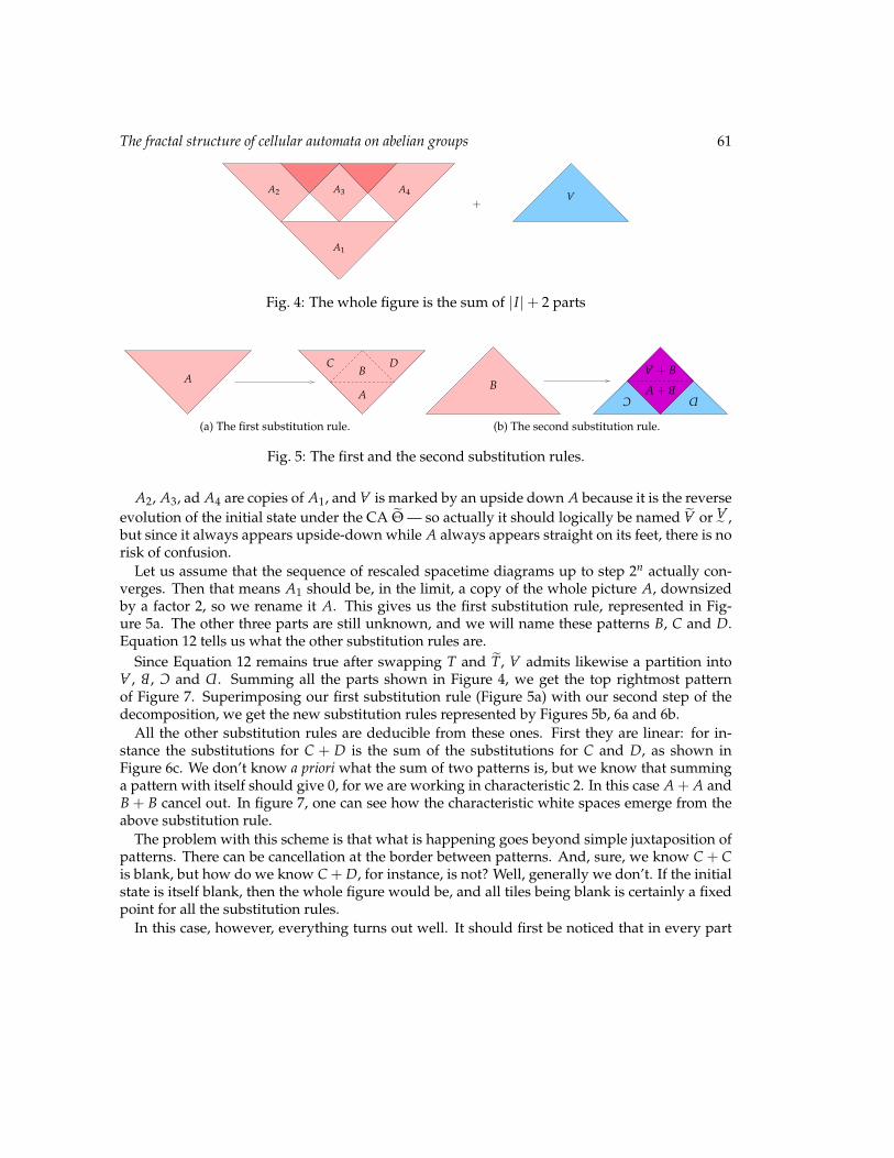
The fractal structure of cellular automata on abelian groups 61
A1
A3A2 A4 A
+
Fig. 4: The whole figure is the sum of |I|+ 2 parts
AA
C DB
(a) The first substitution rule.
D
B
A
+ B
A +
BC
(b) The second substitution rule.
Fig. 5: The first and the second substitution rules.
A2, A3, ad A4 are copies of A1, and
A
is marked by an upside down A because it is the reverseevolution of the initial state under the CA Θ — so actually it should logically be named ˜A
or
A
,but since it always appears upside-down while A always appears straight on its feet, there is norisk of confusion.
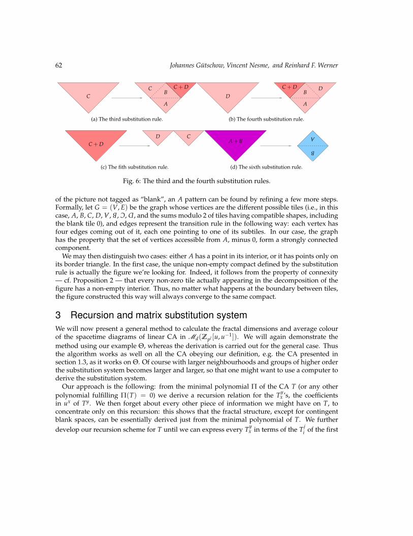
Let us assume that the sequence of rescaled spacetime diagrams up to step 2n actually con-verges. Then that means A1 should be, in the limit, a copy of the whole picture A, downsizedby a factor 2, so we rename it A. This gives us the first substitution rule, represented in Fig-ure 5a. The other three parts are still unknown, and we will name these patterns B, C and D.Equation 12 tells us what the other substitution rules are.
Since Equation 12 remains true after swapping T and T,
A
admits likewise a partition intoA
,
B
,
C
and
D
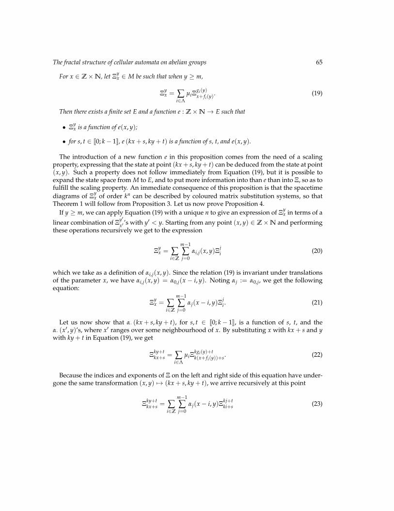
. Summing all the parts shown in Figure 4, we get the top rightmost patternof Figure 7. Superimposing our first substitution rule (Figure 5a) with our second step of thedecomposition, we get the new substitution rules represented by Figures 5b, 6a and 6b.
All the other substitution rules are deducible from these ones. First they are linear: for in-stance the substitutions for C + D is the sum of the substitutions for C and D, as shown inFigure 6c. We don’t know a priori what the sum of two patterns is, but we know that summinga pattern with itself should give 0, for we are working in characteristic 2. In this case A + A andB + B cancel out. In figure 7, one can see how the characteristic white spaces emerge from theabove substitution rule.
The problem with this scheme is that what is happening goes beyond simple juxtaposition ofpatterns. There can be cancellation at the border between patterns. And, sure, we know C + Cis blank, but how do we know C + D, for instance, is not? Well, generally we don’t. If the initialstate is itself blank, then the whole figure would be, and all tiles being blank is certainly a fixedpoint for all the substitution rules.
In this case, however, everything turns out well. It should first be noticed that in every part
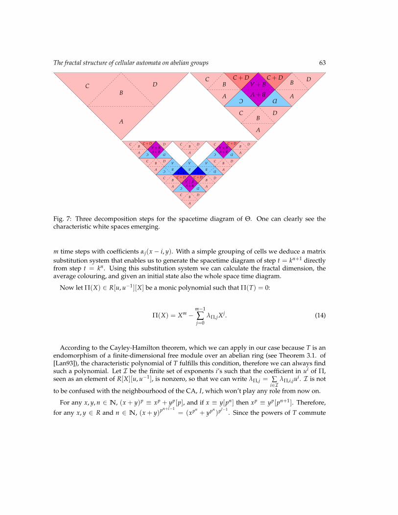
62 Johannes Gutschow, Vincent Nesme, and Reinhard F. Werner
CA
CB
C + D
(a) The third substitution rule.
A
BD
D
C + D
(b) The fourth substitution rule.
D CC + D
(c) The fith substitution rule.
B
A
A +
B
(d) The sixth substitution rule.
Fig. 6: The third and the fourth substitution rules.
of the picture not tagged as “blank”, an A pattern can be found by refining a few more steps.Formally, let G = (V, E) be the graph whose vertices are the different possible tiles (i.e., in thiscase, A, B, C, D,
A
,
B
,
C
,
D
, and the sums modulo 2 of tiles having compatible shapes, includingthe blank tile 0), and edges represent the transition rule in the following way: each vertex hasfour edges coming out of it, each one pointing to one of its subtiles. In our case, the graphhas the property that the set of vertices accessible from A, minus 0, form a strongly connectedcomponent.
We may then distinguish two cases: either A has a point in its interior, or it has points only onits border triangle. In the first case, the unique non-empty compact defined by the substitutionrule is actually the figure we’re looking for. Indeed, it follows from the property of connexity— cf. Proposition 2 — that every non-zero tile actually appearing in the decomposition of thefigure has a non-empty interior. Thus, no matter what happens at the boundary between tiles,the figure constructed this way will always converge to the same compact.
3 Recursion and matrix substitution systemWe will now present a general method to calculate the fractal dimensions and average colourof the spacetime diagrams of linear CA in Md(Zpl [u, u−1]). We will again demonstrate themethod using our example Θ, whereas the derivation is carried out for the general case. Thusthe algorithm works as well on all the CA obeying our definition, e.g. the CA presented insection 1.3, as it works on Θ. Of course with larger neighbourhoods and groups of higher orderthe substitution system becomes larger and larger, so that one might want to use a computer toderive the substitution system.
Our approach is the following: from the minimal polynomial Π of the CA T (or any otherpolynomial fulfilling Π(T) = 0) we derive a recursion relation for the Ty
x ’s, the coefficientsin ux of Ty. We then forget about every other piece of information we might have on T, toconcentrate only on this recursion: this shows that the fractal structure, except for contingentblank spaces, can be essentially derived just from the minimal polynomial of T. We furtherdevelop our recursion scheme for T until we can express every Ty
x in terms of the T ji of the first
The fractal structure of cellular automata on abelian groups 63
C C + DB D
B
A +
BD
CB
D
A
A C
A
+ BC + D
A
A
BC D
C DA A
B BC D
CA DB B B
A
B
A A A
BDCDC
C DA A C D
DB
CDB
CDB
C
A +
B
A +
BA
+ B
A
+ B
A
+ BA +
B
C + D C + D
C
+
D
C + D
C
+
D
C + D
A
CB
D
A
Fig. 7: Three decomposition steps for the spacetime diagram of Θ. One can clearly see thecharacteristic white spaces emerging.
m time steps with coefficients αj(x − i, y). With a simple grouping of cells we deduce a matrixsubstitution system that enables us to generate the spacetime diagram of step t = kn+1 directlyfrom step t = kn. Using this substitution system we can calculate the fractal dimension, theaverage colouring, and given an initial state also the whole space time diagram.
Now let Π(X) ∈ R[u, u−1][X] be a monic polynomial such that Π(T) = 0:
Π(X) = Xm −m−1
∑j=0
λΠ,jX j. (14)
According to the Cayley-Hamilton theorem, which we can apply in our case because T is anendomorphism of a finite-dimensional free module over an abelian ring (see Theorem 3.1. of[Lan93]), the characteristic polynomial of T fulfills this condition, therefore we can always findsuch a polynomial. Let I be the finite set of exponents i’s such that the coefficient in ui of Π,seen as an element of R[X][u, u−1], is nonzero, so that we can write λΠ,j = ∑
i∈IλΠ,i,jui. I is not
to be confused with the neighbourhood of the CA, I, which won’t play any role from now on.
For any x, y, n ∈ N, (x + y)p ≡ xp + yp[p], and if x ≡ y[pn] then xp ≡ yp[pn+1]. Therefore,
for any x, y ∈ R and n ∈ N, (x + y)pn+l−1= (xpn
+ ypn)pl−1
. Since the powers of T commute

64 Johannes Gutschow, Vincent Nesme, and Reinhard F. Werner
pairwise, we get
Tpn+2(l−1)m =
(m−1
∑j=0
λpn+l−1
Π,j Tpn+l−1 j
)pl−1
=
m−1
∑j=0
(∑i∈I
λpn
Π,i,jupni
)pl−1
Tpn+l−1 j
pl−1
. (15)
For each i, j, the sequence λpn
Π,i,j is ultimately periodic. There exists therefore integers N and
M such that for all i, j, λpM+N
Π,i,j = λpM
Π,i,j. Let k = pN ; substituting n by M + Nn in (15), we get
Tkn pM+2(l−1)m =
m−1
∑j=0
(∑i∈I
λpM
Π,i,jukn pM i
)pl−1
Tkn pM+l−1 j
pl−1
. (16)
Hence, if we note m′ = pM+2(l−1)m and expand this equation, we find that there is some finitesubset I ′ of Z and some elements µi,j of R, for i ∈ I ′ and j ∈ J0; m′ − 1K, such that for all n ∈N,
Tknm′ =m′−1
∑j=0
∑i∈I ′
µi,jukniTkn j. (17)
We have now used everything we needed to know from the multiplicative structure on thering of matrices. As announced at the end of section 1.2, we will now get rid of it and con-centrate only on the linear recurrence relation that we have just derived. Remember that T j ∈Md
(R[u, u−1]), and we are interested in the coefficient of T j in ui, denoted T j
i , so that T j =
∑i∈I
T ji ui. We thus get the following relation: Tknm′+y
x = ∑i∈I ′ ∑m′−1j=0 µi,jT
y+kn jx−kni , which we rewrite
in this form:
Tyx = ∑
(i,j)∈I ′×J0;m′−1Kµi,jT
gi,j(y)x+ fi,j(y)
(18)
where fi,j(y) = −kni and gi,j(y) = y − kn(m′ − j), which of course works with any n, butwe will choose n =
⌊logk
ym′⌋. In order to emphasise that the rest of the proof will use only a
minimal structure, we state in the next proposition what will actually be proven, and change thenotation from T, which was an element of Md
(R[u, u−1]
), to Ξ, an element of a more arbitrary
R-module. It is straightforward to check that T fulfils the hypotheses of the proposition.
Proposition 4 Let M be a finite R-module, k a positive integer, Λ a finite set of indices, and for i ∈ Λ,µi ∈ R, fi : Jm;+∞J→ Z and gi : Jm;+∞J→N such that for all y ∈ Jm;+∞J and t ∈ J0; k− 1K,
• gi(y) < y;
• fi(ky + t) = k fi(y) and gi(ky + t) = kgi(y) + t.
The fractal structure of cellular automata on abelian groups 65
For x ∈ Z×N, let Ξyx ∈ M be such that when y ≥ m,
Ξyx = ∑
i∈ΛµiΞ
gi(y)x+ fi(y)
. (19)
Then there exists a finite set E and a function e : Z×N→ E such that
• Ξyx is a function of e(x, y);
• for s, t ∈ J0; k− 1K, e (kx + s, ky + t) is a function of s, t, and e(x, y).
The introduction of a new function e in this proposition comes from the need of a scalingproperty, expressing that the state at point (kx + s, ky + t) can be deduced from the state at point(x, y). Such a property does not follow immediately from Equation (19), but it is possible toexpand the state space from M to E, and to put more information into than e than into Ξ, so as tofulfill the scaling property. An immediate consequence of this proposition is that the spacetimediagrams of Ξy
x of order kn can be described by coloured matrix substitution systems, so thatTheorem 1 will follow from Proposition 3. Let us now prove Proposition 4.
If y ≥ m, we can apply Equation (19) with a unique n to give an expression of Ξyx in terms of a
linear combination of Ξy′
x′ ’s with y′ < y. Starting from any point (x, y) ∈ Z×N and performingthese operations recursively we get to the expression
Ξyx = ∑
i∈Z
m−1
∑j=0
αi,j(x, y)Ξji (20)
which we take as a definition of αi,j(x, y). Since the relation (19) is invariant under translationsof the parameter x, we have αi,j(x, y) = α0,j(x − i, y). Noting αj := α0,j, we get the followingequation:
Ξyx = ∑
i∈Z
m−1
∑j=0
αj(x− i, y)Ξji . (21)
Let us now show that α· (kx + s, ky + t), for s, t ∈ J0; k− 1K, is a function of s, t, and theα· (x′, y)’s, where x′ ranges over some neighbourhood of x. By substituting x with kx + s and ywith ky + t in Equation (19), we get
Ξky+tkx+s = ∑
i∈ΛµiΞ
kgi(y)+tk(x+ fi(y))+s. (22)
Because the indices and exponents of Ξ on the left and right side of this equation have under-gone the same transformation (x, y) 7→ (kx + s, ky + t), we arrive recursively at this point
Ξky+tkx+s = ∑
i∈Z
m−1
∑j=0
αj(x− i, y)Ξkj+tki+s (23)
66 Johannes Gutschow, Vincent Nesme, and Reinhard F. Werner
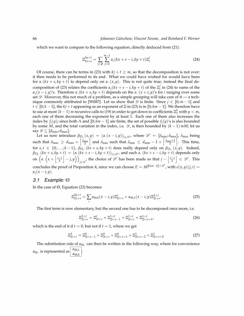
which we want to compare to the following equation, directly deduced from (21):
Ξky+tkx+s = ∑
i∈Z
m−1
∑j=0
αj(kx + s− i, ky + t)Ξji (24)
Of course, there can be terms in (23) with kj + t ≥ m, so that the decomposition is not over:it then needs to be performed to its end. What we could have wished for would have beenfor α·(kx + s, ky + t) to depend only on α· (x, y). This is not quite true; instead the final de-composition of (23) relates the coefficients αj(kx + s− i, ky + t) of the Ξj
i in (24) to sums of theαj(x − i, y)’s. Therefore α·(kx + s, ky + t) depends on the α· (x + i, y)’s for i ranging over someset D . However, this not much of a problem, as a simple grouping will take care of it — a tech-nique commonly attributed to [Wil87]. Let us show that D is finite. Since j ∈ J0; m− 1K andt ∈ J0; k− 1K, the kj + t appearing as an exponent of Ξ in (23) is in J0; km− 1K. We therefore haveto use at most (k− 1)m recursive calls to (19) in order to get down to coefficients Ξy
x with y < m,each one of them decreasing the exponent by at least 1. Each one of them also increases theindex by fi(y); since both Λ and J0; km− 1K are finite, the set of possible fi(y)’s is also boundedby some M, and the total variation in the index, i.e. D , is then bounded by (k− 1)mM; let ussay D ⊆ Jdmin; dmaxK.
Let us now introduce βΠ,·(x, y) = (α·(x− i, y))i∈D ′ , where D ′ = Jδmin; δmaxK, δmax being
such that δmax ≥ dmax +⌈
δmaxk
⌉and δmin such that δmin ≤ dmin − 1 +
⌈δmin+1
k
⌉. This time,
for s, t ∈ {0; . . . ; k− 1}, βΠ,· (kx + s, ky + t) does really depend only on βΠ,· (x, y). Indeed,βΠ,· (kx + s, ky + t) = (α·(kx + s− i, ky + t))i∈D ′ , and each α· (kx + s− i, ky + t) depends only
on(
α·(
x +⌊
s−ik
⌋− j, y
))j∈D
; the choice of D ′ has been made so that j −⌊
s−ik
⌋∈ D ′. This
concludes the proof of Proposition 4, since we can choose E = MJ0;m−1K×D ′ , with e(x, y)(j, i) =αj(x− i, y).
3.1 Example: ΘIn the case of Θ, Equation (23) becomes
Ξ2y+t2x+s = ∑
iαΘ,0(x− i, y)Ξt
2i+s + αΘ,1(x− i, y)Ξ2+t2i+s. (25)
The first term is now elementary, but the second one has to be decomposed once more, i.e.
Ξ2+t2i+s = Ξt
2i+s + Ξ1+t2i+s−1 + Ξ1+t
2i+s + Ξ1+t2i+s+1, (26)
which is the end of it if t = 0, but not if t = 1, where we get
Ξ32i+s = Ξ0
2i+s−1 + Ξ02i+s + Ξ0
2i+s+1 + Ξ12i+s−2 + Ξ1
2i+s+2. (27)
The substitution rule of αΘ,· can then be written in the following way, where for convenience
αΘ,· is represented as αΘ,1αΘ,0
:

The fractal structure of cellular automata on abelian groups 67
αΘ,·(x, y) → αΘ,·(2x, 2y + 1) αΘ,·(2x + 1, 2y + 1)αΘ,·(2x, 2y) αΘ,·(2x + 1, 2y)
=
αΘ,0 (x, y) + αΘ,1 (x− 1, y) + αΘ,1 (x + 1, y)αΘ,1(x, y)
0αΘ,1(x, y) + αΘ,1(x + 1, y)
αΘ,1(x, y)αΘ,0 (x, y) + αΘ,1 (x, y)
αΘ,1(x, y) + αΘ,1(x + 1, y)0
If we follow exactly what has been said in the general case, we ought to consider the grouping{−2; · · · ; 3}. However, this general bound is obviously too rough in the case of Θ, where wewill just have to take {−1; 2}. We will represent the grouping in the form
αΘ,1(x− 1, y) αΘ,1(x, y) αΘ,1(x + 1, y) αΘ,1(x + 2, y)αΘ,0(x− 1, y) αΘ,0(x, y) αΘ,0(x + 1, y) αΘ,0(x + 2, y) .
The alphabet has thus size 256, and the substitution system is described by
a b c de f g h →
0 a + c + f 0 b + d + ga + b b b + c c
a + c + f 0 b + d + g 0b b + c c c + d
a + b b b + c c0 b + f 0 c + g
b b + c c c + db + f 0 c + g 0
Let us denote by A the matrix having a 1 in position a and 0 elsewhere, B the matrix havinga 1 only in position b, and so on. For these matrices, we will denote the sum of matrices by asimple juxtaposition: AB will mean A + B, as the matrix multiplication has no meaning in thiscontext.
Since T0x = δx0T0
0 , the starting position, with which we describe the whole line number 0,
is · · · 0 H G F E 0 · · · . Since we have, for instance, the rule F → B AF E , the
graph derived from this substitution system is aperiodic; that means that, in whatever wayA, B, C, . . . are represented, either as coloured dots or as white dots, the pattern converges, andthe fractal structure is described by this matrix substitution system (see Section 1.4).
To calculate the fractal dimension of our spacetime diagram we use the transition matrix of thematrix substitution system, which contains the information about the images of all states. Theline corresponding to F would contain a 1 in the rows of A, B, E, and F and zeros elsewhere. Asevery cell gives rise to four new cells the sum of all entries in each column of the matrix is 4. Wethus deal with a sparse 256× 256 matrix. The base 2 logarithm of the second largest eigenvalueof this matrix is the fractal dimension of the spacetime diagram (cf. for instance [Wil87]). Herethis gives a fractal dimension of log2
3+√
172 ' 1.8325, as also found in [Mac04].
Let us note that up to this point our analysis for Θ is word for word valid for all CA inM2(Z2[u, u−1]) of determinant 1 and trace u−1 + 1+ u. The additional information is only usedfor the actual colouring of the picture. In general all CA with the same minimal polynomial havethe same substitution system, and in dimension 2 the minimal polynomial is entirely determinedby the trace and the determinant. The fractal we get if we use the substitution system startingfrom · · · 0 H G F E 0 · · · is shown in Figure 8.
68 Johannes Gutschow, Vincent Nesme, and Reinhard F. Werner
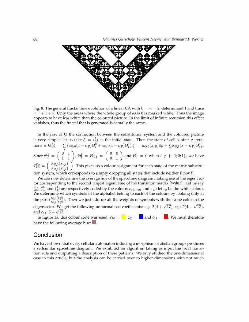
Fig. 8: The general fractal time evolution of a linear CA with k = m = 2, determinant 1 and traceu−1 + 1 + u. Only the areas where the whole group of αs is 0 is marked white. Thus the imageappears to have less white than the coloured picture. In the limit of infinite recursion this effectvanishes, thus the fractal that is generated is actually the same.
In the case of Θ the connection between the substitution system and the coloured pictureis very simple; let us take ξ = (1
0) as the initial state. Then the state of cell x after y itera-tions is Θy
xξ = ∑i
(αΘ,0(x− i, y)Θ0
i + αΘ,1(x− i, y)Θ1i)
ξ = αΘ,0(x, y)1ξ + ∑i
αΘ,1(x − i, y)Θ1i ξ.
Since Θ10 =
(0 11 1
), Θ1
1 = Θ1−1 =
(0 00 1
)and Θ1
i = 0 when i 6∈ {−1; 0; 1}, we have
Tyx ξ =
(αΘ,0(x, y)αΘ,1(x, y)
). This gives us a colour assignment for each state of the matrix substitu-
tion system, which corresponds to simply dropping all states that include neither B nor F.We can now determine the average hue of the spacetime diagram making use of the eigenvec-
tor corresponding to the second largest eigenvalue of the transition matrix [Wil87]. Let us say(1
0), (01) and (1
1) are respectively coded by the colours c10, c01 and c11; let cq be the white colour.We determine which symbols of the alphabet belong to each of the colours by looking only atthe part (αΘ,0(x,y)
αΘ,1(x,y)). Then we just add up all the weights of symbols with the same color in the
eigenvector. We get the following unnormalised coefficients: c10: 2(4 +√
17), c01: 2(4 +√
17),and c11: 5 +
√17.
In figure 1a, this colour code was used: c10 = , c01 = and c11 = . We must thereforehave the following average hue: .
ConclusionWe have shown that every cellular automaton inducing a morphism of abelian groups producesa selfsimilar spacetime diagram. We exhibited an algorithm taking as input the local transi-tion rule and outputting a description of these patterns. We only studied the one-dimensionalcase in this article, but the analysis can be carried over to higher dimensions with not much

The fractal structure of cellular automata on abelian groups 69
more ado. Instead of Md(
R[u, u−1]), a n-dimensional linear cellular automaton would then
be an element of Md(R[u1, u−11 , u2, u−1
2 , . . . un, u−1n ]), matrix substitution systems would become
(n + 1)-dimensional array substitution systems, the system of indices in section 3 would befurther complicated, and the spacetime diagrams would be harder to display. However, thegeneralisation does not present any theoretical difficulty.
We list here some open questions and possible future developments.
• Possibly, the m in Theorem 1 can always be taken to be 1. This is known to be true in thecyclic case, i.e. when d = 1, cf [Tak92].
• The algorithm presented in this article, producing a description of the spacetime diagramin the form of a matrix substition system, has a high complexity, due to the large size ofits output. Is this a necessary evil, or can more efficient descriptions be found? Couldfor instance the more elegant triangle-based substitution scheme presented in section 2 benaturally generalised?
• To what extent can the algebraic structure be weakened? Instead of the alphabet being anabelian group, could we consider an abelian monoid? Is it possible to get rid of commuta-tivity and/or associativity?
AcknowledgementsThe authors would like to thank Jean-Paul Allouche, Bruno Durand, Cris Moore and VolkherScholz for their useful feedback and bibliographical hints. They also gratefully acknowledgethe support of the Deutsche Forschungsgemeinschaft (Forschergruppe 635), the EU (projectsCORNER and QICS), the Erwin Schrodinger Institute and the Rosa Luxemburg Foundation.
References[AHP+97] Jean-Paul Allouche, Fritz von Haeseler, Heinz-Otto Peitgen, A. Petersen, and
Guentcho Skordev. Automaticity of double sequences generated by one-dimensional linear cellular automata. Theoretical Computer Science, 188(1–2):195–209,November 1997.
[AHPS96] Jean-Paul Allouche, Fritz von Haeseler, Heinz-Otto Peitgen, and Guentcho Skordev.Linear cellular automata, finite automata and Pascal’s triangle. Discrete AppliedMathematics, 66(1):1–22, April 1996.
[Gut10] Johannes Gutschow. Entanglement generation of Clifford quantum cellular au-tomata. Applied Physics B, 98(4):623–633, March 2010.
[GUWZ10] Johannes Gutschow, Sonja Uphoff, Reinhard F. Werner, and Zoltan Zimboras. Timeasymptotics and entanglement generation of Clifford quantum celluar automata.Journal of Mathematical Physics, 51(1), January 2010.
70 Johannes Gutschow, Vincent Nesme, and Reinhard F. Werner
[HPS93] Fritz von Haeseler, Heinz-Otto Peitgen, and Guentcho Skordev. Cellular automata,matrix substitutions and fractals. Annals of Mathematics and Artificial Intelligence,8(3–4):345–362, September 1993.
[HPS01] Fritz von Haeseler, Heinz-Otto Peitgen, and Guentcho Skordev. Self-similar struc-ture of rescaled evolution sets of cellular automata. International Journal of Bifurcationand Chaos, 11(4):913–941, 2001.
[Lan93] Serge Lang. Algebra. Addison-Wesley publishing company, third edition, 1993.
[Mac04] Alan J. Macfarlane. Linear reversible second-order cellular automata and their first-order matrix equivalents. Journal of Physics A: Mathematical and General, 37:10791–10814, 2004.
[Mac09] Alan J. Macfarlane. On the evolution of the cellular automaton of rule 150 fromsome simple initial states. Journal of Mathematical Physics, 50(6):062702, 2009.
[MGAP85] Benoıt B. Mandelbrot, Yuval Gefen, Amnon Aharony, and Jacques Peyrire. Fractals,their transfer matrices and their eigen-dimensional sequences. Journal of Physics A:Mathematical and General, 18:335–354, 1985.
[Moo97] Cristopher Moore. Quasi-linear cellular automata. Physica D, 103:100–132, 1997.
[Moo98] Cristopher Moore. Non-abelian cellular automata. Physica D, 111:27–41, 1998.
[MOW84] Olivier Martin, Andrew M. Odlyzko, and Stephen Wolfram. Algebraic properties ofcellular automata. Communications in Mathematical Physics, 93:219–258, March 1984.
[SVW08] Dirk M. Schlingemann, Holger Vogts, and Reinhard F. Werner. On the structure ofClifford quantum cellular automata. Journal of Mathematical Physics, 49, 2008.
[Tak90] Satoshi Takahashi. Cellular automata and multifractals: dimension spectra linearcellular automata. Physica D, 45(1-3):36–48, 1990.
[Tak92] Satoshi Takahashi. Self-similarity of linear cellular automata. Journal of Computerand System Sciences, 44(1):114–140, 1992.
[Wil87] Stephen J. Willson. Computing fractal dimensions for additive cellular automata.Physica D, 24:190–206, 1987.