the fourier transform - utkweb.eecs.utk.edu/~mjr/ece503/presentationslides/chapter5slides.pdfof the...

The Fourier Transform

5/10/04 M. J. Roberts - All Rights Reserved 2

Extending the CTFS

• The CTFS is a good analysis tool for systemswith periodic excitation but the CTFS cannotrepresent an aperiodic signal for all time

• The continuous-time Fourier transform(CTFT) can represent an aperiodic signal forall time


CTFS-to-CTFT Transition

Its CTFS harmonic function is X sinckAwT

kwT

[ ] =

0 0

Consider a periodic pulse-train signal, x(t), with duty cycle, wT0

As the period, , is increased, holding w constant, the duty cycle is decreased. When the period becomes infinite (and the duty cycle becomes zero) x(t) is no longer periodic.

T0


CTFS-to-CTFT Transition

wT= 0

2 wT= 0

10

Below are plots of the magnitude of X[k] for 50% and 10% dutycycles. As the period increases the sinc function widens and itsmagnitude falls. As the period approaches infinity, the CTFSharmonic function becomes an infinitely-wide sinc function withzero amplitude.


CTFS-to-CTFT TransitionThis infinity-and-zero problem can be solved by normalizing the CTFS harmonic function. Define a new “modified” CTFS harmonic function,

T k Aw w kf0 0X sinc[ ] = ( )( )and graph it versus instead of versus k.kf0


CTFS-to-CTFT TransitionIn the limit as the period approaches infinity, the modifiedCTFS harmonic function approaches a function of continuousfrequency f ( ).kf0


Forward Inverse

X x xf t t e dtj ft( ) = ( )( ) = ( ) −

−∞

∞

∫F 2π

x X X-1t f f e dfj ft( ) = ( )( ) = ( ) +

−∞

∞

∫F 2π

f form

X xj t x t e dtj tω ω( ) = ( )( ) = ( ) −

−∞

∞

∫F x X X-1t j j e dj t( ) = ( )( ) = ( ) +

−∞

∞

∫F ωπ

ω ωω12

ω formForward Inverse

Definition of the CTFT

x Xt f( )← → ( )F x Xt j( )← → ( )F ωor

Commonly-used notation:


Some Remarkable Implicationsof the Fourier Transform

The CTFT expresses a finite-amplitude, real-valued, aperiodic signal which can also, in general, be time-limited, as a summation (an integral) of an infinite continuum of weighted, infinitesimal-amplitude, complex sinusoids, each of which is unlimited intime. (Time limited means “having non-zero values only for afinite time.”)


Frequency Content

Lowpass Highpass

Bandpass


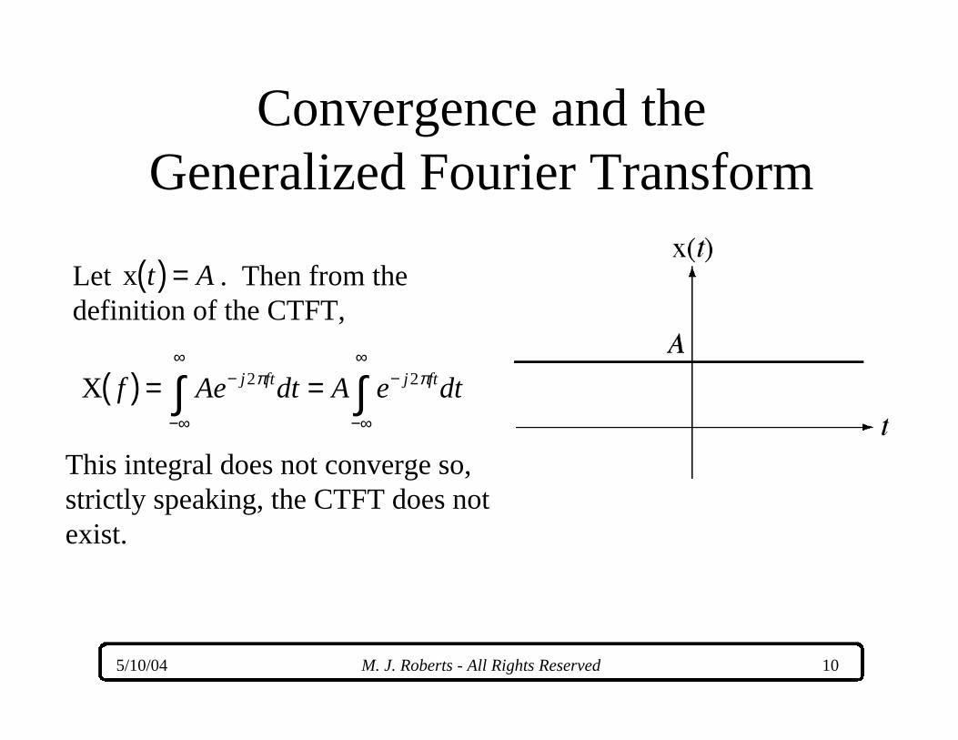
Convergence and theGeneralized Fourier Transform

Let . Then from the definition of the CTFT,

x t A( ) =

X f Ae dt A e dtj ft j ft( ) = =−

−∞

∞−

−∞

∞

∫ ∫2 2π π

This integral does not converge so, strictly speaking, the CTFT does not exist.


Convergence and the GeneralizedFourier Transform

x ,σσ σt Ae t( ) = >− 0

Its CTFT integral,

does converge.

Xσσ πf Ae e dtt j ft( ) = − −

−∞

∞

∫ 2

But consider a similar function,



Carrying out the integral, . Xσσ

σ πf A

f( ) =

+( )2

22 2

If then . The area under thisfunction is

f ≠ 0 limσ

σσ π→ +( )

=0 2 2

2

20A

f

Area =+( )−∞

∞

∫Af

df2

22 2

σσ π

which is A, independent of the value of σ. So, in the limit as

σ approaches zero, the CTFT has an area of A and is zero unless

. This exactly defines an impulse of strength, A. Therefore

f = 0

A A fF← → ( )δ

Now let σ approach zero.



By a similar process it can be shown that

cos 2

120 0 0π δ δf t f f f f( )← → −( ) + +( )[ ]F

and

sin 2

20 0 0π δ δf tj

f f f f( )← → +( ) − −( )[ ]F

These CTFT’s which involve impulses are called generalized Fourier transforms (probably becausethe impulse is a generalized function).


Convergence and the GeneralizedFourier Transform


Negative FrequencyThis signal is obviously a sinusoid. How is it describedmathematically?

It could be described by

x cos cost At

TA f t( ) =

= ( )22

00

π π

But it could also be described by

x cost A f t( ) = −( )( )2 0π


Negative Frequency

x(t) could also be described by

x cos cos ,t A f t A f t A A A( ) = ( ) + −( )( ) + =1 0 2 0 1 22 2π π

x t Ae ej f t j f t

( ) = + −2 20 0

2

π π

and probably in a few other different-looking ways. So who isto say whether the frequency is positive or negative? For thepurposes of signal analysis, it does not matter.

or


CTFT PropertiesIf F Fx X X and y Y Yt f j t f j( )( ) = ( ) ( ) ( )( ) = ( ) ( )or orω ωthen the following properties can be proven.

Linearity α β α βx y X Yt t f f( )+ ( )← → ( )+ ( )F

α β α ω β ωx y X Yt t j j( )+ ( )← → ( )+ ( )F


CTFT Properties

Time Shifting

x Xt t f e j ft−( )← → ( ) −0

2 0F π

x Xt t j e j t−( )← → ( ) −0

0F ω ω


CTFT Properties

x Xt e f fj f t( ) ← → −( )+ 20

0π F

Frequency Shifting

x Xt e j t( ) ← → −( )+ ω ω ω00

F


CTFT Properties

Time Scaling x Xat

afa

( )← →

F 1

x Xat

aj

a( )← →

F 1 ω

Frequency Scaling 1a

ta

afx X

← → ( )F

1a

ta

jax X

← → ( )F ω


The “Uncertainty” PrincipleThe time and frequency scaling properties indicate that if a signal is expanded in one domain it is compressed in the other domain.This is called the “uncertainty principle” of Fourier analysis.

e et

f−

− ( )← →

π π2 2

2

2

2F

e et f− −← →π π2 2F e et f− −← →π π2 2

2F


CTFT Properties

Transform of a Conjugate

x X* *t f( )← → −( )F

x X* *t j( )← → −( )F ω

Multiplication-Convolution

Duality

x y X Yt t f f( )∗ ( )← → ( ) ( )F

x y X Yt t j j( )∗ ( )← → ( ) ( )F ω ω

x y X Yt t f f( ) ( )← → ( )∗ ( )F

x y X Yt t j j( ) ( )← → ( )∗ ( )F 1

2πω ω


CTFT Properties


CTFT PropertiesAn important consequence of multiplication-convolutionduality is the concept of the transfer function.

In the frequency domain, the cascade connection multipliesthe transfer functions instead of convolving the impulseresponses.


CTFT Properties

Time Differentiation

ddt

t j f fx X( )( )← → ( )F 2π

ddt

t j jx X( )( )← → ( )F ω ω

Modulation x cos X Xt f t f f f f( ) ( )← → −( ) + +( )[ ]2

120 0 0π F

x cos X Xt t j j( ) ( )← → −( )( ) + +( )( )[ ]ω ω ω ω ω0 0 0

12

F

Transforms ofPeriodic Signals

x X X Xt k e f k f kfj kf t

k k

F( ) = [ ] ← → ( ) = [ ] −( )− ( )

=−∞

∞

=−∞

∞

∑ ∑20

π δF

x X X Xt k e j k kj k t

k k

F( ) = [ ] ← → ( ) = [ ] −( )− ( )

=−∞

∞

=−∞

∞

∑ ∑ω ω π δ ω ωF 2 0


CTFT Properties


CTFT Properties

Parseval’s Theorem

x Xt dt f df( ) = ( )−∞

∞

−∞

∞

∫ ∫2 2

x Xt dt j df( ) = ( )−∞

∞

−∞

∞

∫ ∫2 212π

ω

Integral Definitionof an Impulse

e dy xj xy−

−∞

∞

∫ = ( )2π δ

Duality X x X xt f t f( )← → −( ) −( )← → ( )F Fand

X x X xjt jt( )← → −( ) −( )← → ( )F F2 2π ω π ωand


CTFT Properties

Total-AreaIntegral

X x x0 2

0

( ) = ( )

= ( )−

−∞

∞

→ −∞

∞

∫ ∫t e dt t dtj ft

f

π

x X X0 2

0

( ) = ( )

= ( )+

−∞

∞

→ −∞

∞

∫ ∫f e df f dfj ft

t

π

X x x00

( ) = ( )

= ( )−

−∞

∞

→ −∞

∞

∫ ∫t e dt t dtj tω

ω

x X X01

21

20

( ) = ( )

= ( )+

−∞

∞

→ −∞

∞

∫ ∫πω ω

πω ωωj e d j dj t

t

Integration x

XXλ λ

πδ( ) ← → ( ) + ( ) ( )

−∞∫ d

fj f

ft

F

212

0

x

XXλ λ ω

ωπ δ ω( ) ← → ( ) + ( ) ( )

−∞∫ d

jj

tF 0


CTFT Properties

x X0( ) = ( )−∞

∞

∫ f df

X x0( ) = ( )−∞

∞

∫ t dt


CTFT Properties


Extending the DTFS

• Analogous to the CTFS, the DTFS is a goodanalysis tool for systems with periodicexcitation but cannot represent an aperiodicDT signal for all time

• The discrete-time Fourier transform (DTFT)can represent an aperiodic DT signal for alltime


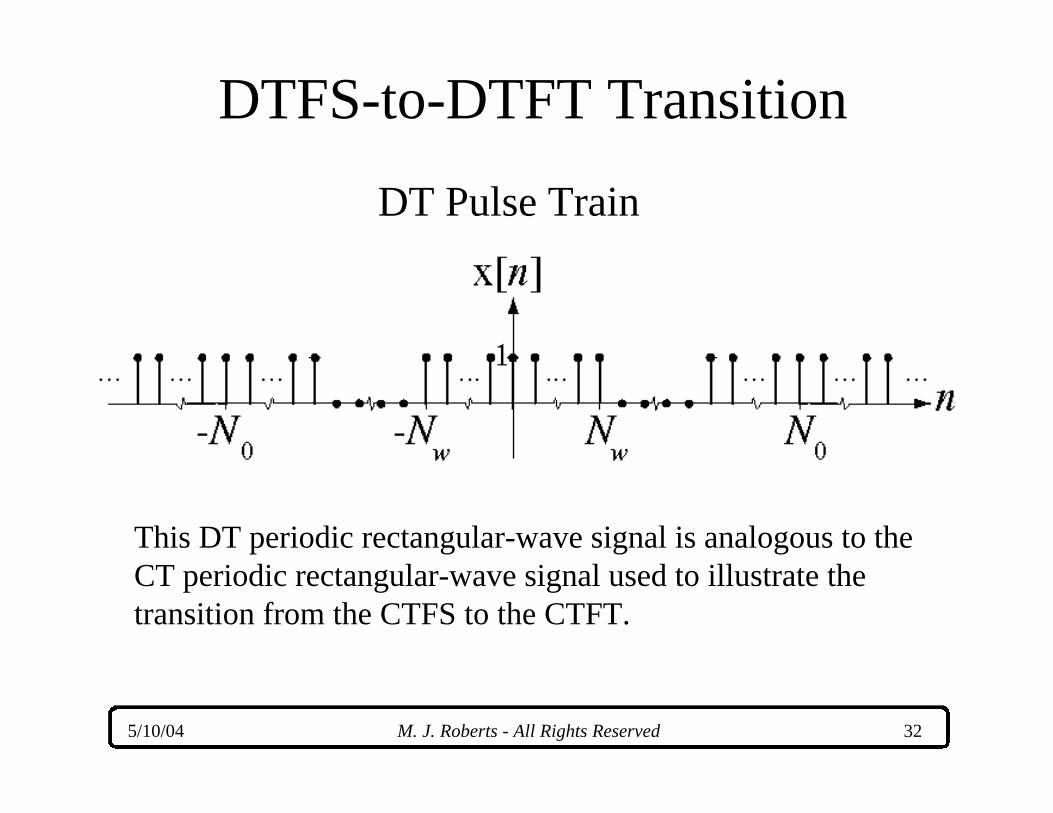
DTFS-to-DTFT Transition

DT Pulse Train

This DT periodic rectangular-wave signal is analogous to theCT periodic rectangular-wave signal used to illustrate the transition from the CTFS to the CTFT.



DTFS of DT Pulse Train

As the period of therectangular waveincreases, the period ofthe DTFS increasesand the amplitude ofthe DTFS decreases.


DTFS-to-DTFT TransitionNormalized

DTFS ofDT Pulse Train

By multiplying theDTFS by its period andplotting versusinstead of k, theamplitude of the DTFSstays the same as theperiod increases andthe period of thenormalized DTFSstays at one.

kF0



The normalized DTFS approaches this limit as the DTperiod approaches infinity.


Definition of the DTFT

x X X xn F e dF F n ej Fn j Fn

n

[ ] = ( ) ← → ( ) = [ ]∫ ∑ −

=−∞

∞2

1

2π πF

F Form

x X X xn j e d j n ej n j n

n

[ ] = ( ) ← → ( ) = [ ]∫ ∑ −

=−∞

∞12 2π π

Ω Ω ΩΩ ΩF

Ω Form

ForwardInverse

ForwardInverse


DTFT Properties

Linearity α β α βx y X Yn n F F[ ] + [ ]← → ( )+ ( )F

α β α βx y X Yn n j j[ ] + [ ]← → ( )+ ( )F Ω Ω


DTFT PropertiesTime

Shifting x Xn n e Fj Fn−[ ] ← → ( )−

02 0F π

x Xn n e jj n−[ ] ← → ( )−0

0F Ω Ω


DTFT Properties

e n F Fj F n20

0π x X[ ]← → −( )F

e n jj nΩ Ω Ω00x X[ ]← → −( )( )F

FrequencyShifting

TimeReversal

x X−[ ]← → −( )n FF

x X−[ ]← → −( )n jF Ω


DTFT Properties x x Xn n e Fj F[ ] − −[ ]← → −( ) ( )−1 1 2F π

Differencing

x x Xn n e jj[ ] − −[ ]← → −( ) ( )−1 1F Ω Ω


DTFT Properties

x

XX combm

Fe

Fm

n

j F[ ]← → ( )−

+ ( ) ( )=−∞

−∑ F

112

02πAccumulation

x

XX combm

jem

n

j[ ]← → ( )−

+ ( )

=−∞−∑ F Ω Ω

Ω112

02π


DTFT Properties

As is true for other transforms, convolution in the time domain is equivalent to multiplication in the frequency domain

Multiplication-Convolution

Duality

x y X Yn n F F[ ] ∗ [ ]← → ( ) ( )F

x y X Yn n j j[ ] ∗ [ ]← → ( ) ( )F Ω Ω

x y X Yn n F F[ ] [ ] ← → ( ) ( )F

x y X Yn n j j[ ] [ ] ← → ( ) ( )F 1

2πΩ Ω


DTFT Properties


DTFT Properties

AccumulationDefinition of a Comb Function

e Fj Fn

n

2π

=−∞

∞

∑ = ( )comb

The signal energy is proportional to the integral of the squared magnitude of the DTFT of the signal over one period.

Parseval’sTheorem x Xn j d

n

[ ] = ( )=−∞

∞

∑ ∫2 2

2

12π π

Ω Ω

x Xn F dFn

[ ] = ( )=−∞

∞

∑ ∫2 2

1


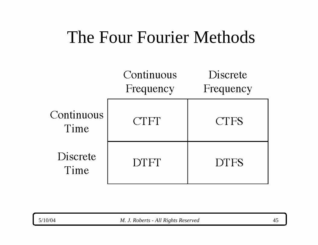
The Four Fourier Methods


Relations Among Fourier MethodsDiscrete Frequency Continuous Frequency

CT

DT


CTFT - CTFS RelationshipX Xf k f kf

k

( ) = [ ] −( )=−∞

∞

∑ δ 0


CTFT - CTFS Relationship

X Xp p pk f kf[ ] = ( )


CTFT - DTFT Relationship

Let x x comb xδ δt tT

tT

nT t nTs s

s sn

( ) = ( )

= ( ) −( )=−∞

∞

∑1

and let x xn nTs[ ] = ( )

X XDTFT sF f F( ) = ( )δ X Xδ fffDTFT

s

( ) =

X XDTFT s CTFT sk

F f f F k( ) = −( )( )=−∞

∞

∑

There is an “information equivalence” between and . They are both completely described bythe same set of numbers.

xδ t( )x n[ ]


CTFT - DTFT Relationship


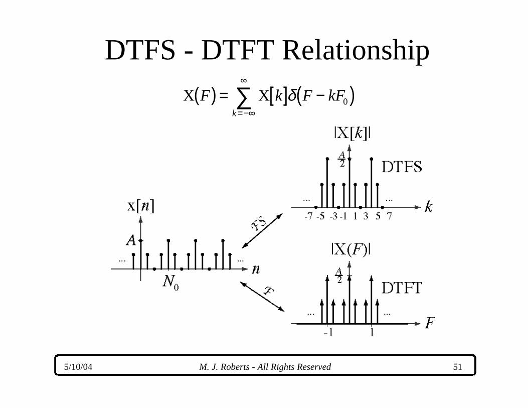
DTFS - DTFT Relationship

X XF k F kFk

( ) = [ ] −( )=−∞

∞

∑ δ 0


DTFS - DTFT Relationship

X Xpp

pkN

kF[ ] = ( )1

the fourier transform - utkweb.eecs.utk.edu/~mjr/ece503/presentationslides/chapter5slides.pdfof the...

Documents