the four types of estimable functions - sas...introduction to reduction notation f 257 since all...

SAS/STAT® 13.1 User’s GuideThe Four Types ofEstimable Functions

This document is an individual chapter from SAS/STAT® 13.1 User’s Guide.

The correct bibliographic citation for the complete manual is as follows: SAS Institute Inc. 2013. SAS/STAT® 13.1 User’s Guide.Cary, NC: SAS Institute Inc.

Copyright © 2013, SAS Institute Inc., Cary, NC, USA

All rights reserved. Produced in the United States of America.

For a hard-copy book: No part of this publication may be reproduced, stored in a retrieval system, or transmitted, in any form or byany means, electronic, mechanical, photocopying, or otherwise, without the prior written permission of the publisher, SAS InstituteInc.

For a web download or e-book: Your use of this publication shall be governed by the terms established by the vendor at the timeyou acquire this publication.

The scanning, uploading, and distribution of this book via the Internet or any other means without the permission of the publisher isillegal and punishable by law. Please purchase only authorized electronic editions and do not participate in or encourage electronicpiracy of copyrighted materials. Your support of others’ rights is appreciated.

U.S. Government License Rights; Restricted Rights: The Software and its documentation is commercial computer softwaredeveloped at private expense and is provided with RESTRICTED RIGHTS to the United States Government. Use, duplication ordisclosure of the Software by the United States Government is subject to the license terms of this Agreement pursuant to, asapplicable, FAR 12.212, DFAR 227.7202-1(a), DFAR 227.7202-3(a) and DFAR 227.7202-4 and, to the extent required under U.S.federal law, the minimum restricted rights as set out in FAR 52.227-19 (DEC 2007). If FAR 52.227-19 is applicable, this provisionserves as notice under clause (c) thereof and no other notice is required to be affixed to the Software or documentation. TheGovernment’s rights in Software and documentation shall be only those set forth in this Agreement.

SAS Institute Inc., SAS Campus Drive, Cary, North Carolina 27513-2414.

December 2013

SAS provides a complete selection of books and electronic products to help customers use SAS® software to its fullest potential. Formore information about our offerings, visit support.sas.com/bookstore or call 1-800-727-3228.

SAS® and all other SAS Institute Inc. product or service names are registered trademarks or trademarks of SAS Institute Inc. in theUSA and other countries. ® indicates USA registration.

Other brand and product names are trademarks of their respective companies.

SAS and all other SAS Institute Inc. product or service names are registered trademarks or trademarks of SAS Institute Inc. in the USA and other countries. ® indicates USA registration. Other brand and product names are trademarks of their respective companies. © 2013 SAS Institute Inc. All rights reserved. S107969US.0613

Discover all that you need on your journey to knowledge and empowerment.

support.sas.com/bookstorefor additional books and resources.

Gain Greater Insight into Your SAS® Software with SAS Books.

Chapter 15

The Four Types of Estimable Functions

ContentsOverview . . . . . . . . . . . . . . . . . . . . . . . . . . . . . . . . . . . . . . . . . . . . 255Estimability . . . . . . . . . . . . . . . . . . . . . . . . . . . . . . . . . . . . . . . . . . . 255

General Form of an Estimable Function . . . . . . . . . . . . . . . . . . . . . . . . . 256Introduction to Reduction Notation . . . . . . . . . . . . . . . . . . . . . . . . . . . 257Examples . . . . . . . . . . . . . . . . . . . . . . . . . . . . . . . . . . . . . . . . . 258

Estimable Functions . . . . . . . . . . . . . . . . . . . . . . . . . . . . . . . . . . . . . . 261Type I SS and Estimable Functions . . . . . . . . . . . . . . . . . . . . . . . . . . . 261Type II SS and Estimable Functions . . . . . . . . . . . . . . . . . . . . . . . . . . . 263Type III and IV SS and Estimable Functions . . . . . . . . . . . . . . . . . . . . . . 266

References . . . . . . . . . . . . . . . . . . . . . . . . . . . . . . . . . . . . . . . . . . . 271

OverviewMany regression and analysis of variance procedures in SAS/STAT label tests for various effects in the modelas Type I, Type II, Type III, or Type IV. These four types of hypotheses might not always be sufficient for astatistician to perform all desired inferences, but they should suffice for the vast majority of analyses. Thischapter explains the hypotheses involved in each of the four test types. For additional discussion, see Freund,Littell, and Spector (1991) or Milliken and Johnson (1984).

The primary context of the discussion is testing linear hypotheses in least squares regression and analysis ofvariance, such as with PROC GLM. In this context, tests correspond to hypotheses about linear functions ofthe true parameters and are evaluated using sums of squares of the estimated parameters. Thus, there will befrequent references to Type I, II, III, and IV (estimable) functions and corresponding Type I, II, III, and IVsums of squares, or simply SS.

EstimabilityGiven a response or dependent variable Y, predictors or independent variables X, and a linear expectationmodel EŒY� D Xˇ relating the two, a primary analytical goal is to estimate or test for the significance ofcertain linear combinations of the elements of ˇ. For least squares regression and analysis of variance, thisis accomplished by computing linear combinations of the observed Ys. An unbiased linear estimate of aspecific linear function of the individual ˇs, say Lˇ, is a linear combination of the Ys that has an expectedvalue of Lˇ. Hence, the following definition:

256 F Chapter 15: The Four Types of Estimable Functions

A linear combination of the parameters Lˇ is estimable if and only if a linear combination of theYs exists that has expected value Lˇ.

Any linear combination of the Ys, for instance KY, will have expectation EŒKY� D KXˇ. Thus, theexpected value of any linear combination of the Ys is equal to that same linear combination of the rows of Xmultiplied by ˇ. Therefore,

Lˇ is estimable if and only if there is a linear combination of the rows of X that is equal toL—that is, if and only if there is a K such that L D KX.

Thus, the rows of X form a generating set from which any estimable L can be constructed. Since the rowspace of X is the same as the row space of X0X, the rows of X0X also form a generating set from which allestimable Ls can be constructed. Similarly, the rows of .X0X/�X0X also form a generating set for L.

Therefore, if L can be written as a linear combination of the rows of X, X0X, or .X0X/�X0X, then Lˇ isestimable.

In the context of least squares regression and analysis of variance, an estimable linear function Lˇ can beestimated by Lb̌, where b̌D .X0X/�X0Y. From the general theory of linear models, the unbiased estimatorLb̌ is, in fact, the best linear unbiased estimator of Lˇ, in the sense of having minimum variance as well asmaximum likelihood when the residuals are normal. To test the hypothesis that Lˇ D 0, compute the sum ofsquares

SS.H0W Lˇ D 0/ D .Lb̌/0.L.X0X/�L0/�1Lb̌and form an F test with the appropriate error term. Note that in contexts more general than least squaresregression (for example, generalized and/or mixed linear models), linear hypotheses are often tested byanalogous sums of squares of the estimated linear parameters .Lb̌/0.VarŒLb̌�/�1Lb̌.

General Form of an Estimable FunctionThis section demonstrates a shorthand technique for displaying the generating set for any estimable L.Suppose

X D

26666664

1 1 0 0

1 1 0 0

1 0 1 0

1 0 1 0

1 0 0 1

1 0 0 1

37777775 and ˇ D

2664�

A1

A2

A3

3775

X is a generating set for L, but so is the smaller set

X� D

24 1 1 0 0

1 0 1 0

1 0 0 1

35X� is formed from X by deleting duplicate rows.

Introduction to Reduction Notation F 257

Since all estimable Ls must be linear functions of the rows of X� for Lˇ to be estimable, an L for asingle-degree-of-freedom estimate can be represented symbolically as

L1 � .1 1 0 0/C L2 � .1 0 1 0/C L3 � .1 0 0 1/

or

L D .L1 C L2 C L3 ; L1 ; L2 ; L3 /

For this example, Lˇ is estimable if and only if the first element of L is equal to the sum of the other elementsof L or if

Lˇ D .L1 C L2 C L3 / � �C L1 � A1 C L2 � A2 C L3 � A3

is estimable for any values of L1, L2, and L3.

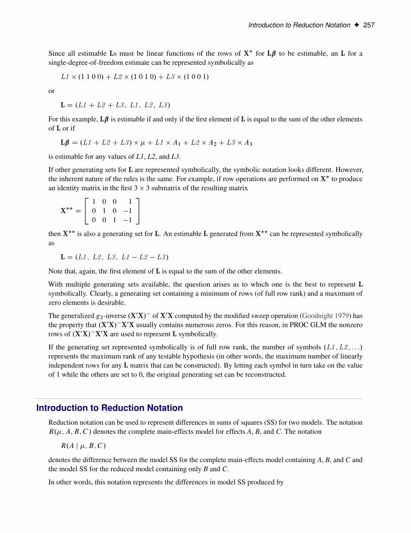
If other generating sets for L are represented symbolically, the symbolic notation looks different. However,the inherent nature of the rules is the same. For example, if row operations are performed on X� to producean identity matrix in the first 3 � 3 submatrix of the resulting matrix

X�� D

24 1 0 0 1

0 1 0 �1

0 0 1 �1

35then X�� is also a generating set for L. An estimable L generated from X�� can be represented symbolicallyas

L D .L1 ; L2 ; L3 ; L1 � L2 � L3 /

Note that, again, the first element of L is equal to the sum of the other elements.

With multiple generating sets available, the question arises as to which one is the best to represent Lsymbolically. Clearly, a generating set containing a minimum of rows (of full row rank) and a maximum ofzero elements is desirable.

The generalized g2-inverse .X0X/� of X0X computed by the modified sweep operation (Goodnight 1979) hasthe property that .X0X/�X0X usually contains numerous zeros. For this reason, in PROC GLM the nonzerorows of .X0X/�X0X are used to represent L symbolically.

If the generating set represented symbolically is of full row rank, the number of symbols .L1 ;L2 ; : : :/represents the maximum rank of any testable hypothesis (in other words, the maximum number of linearlyindependent rows for any L matrix that can be constructed). By letting each symbol in turn take on the valueof 1 while the others are set to 0, the original generating set can be reconstructed.

Introduction to Reduction NotationReduction notation can be used to represent differences in sums of squares (SS) for two models. The notationR.�;A;B; C / denotes the complete main-effects model for effects A, B, and C. The notation

R.A j �;B;C /

denotes the difference between the model SS for the complete main-effects model containing A, B, and C andthe model SS for the reduced model containing only B and C.

In other words, this notation represents the differences in model SS produced by


proc glm;class a b c;model y = a b c;

run;

and

proc glm;class b c;model y = b c;

run;

As another example, consider a regression equation with four independent variables. The notationR.ˇ3; ˇ4 j ˇ1; ˇ2/ denotes the differences in model SS between

y D ˇ0 C ˇ1x1 C ˇ2x2 C ˇ3x3 C ˇ4x4 C �

and

y D ˇ0 C ˇ1x1 C ˇ2x2 C �

This is the difference in the model SS for the models produced, respectively, by

model y = x1 x2 x3 x4;

and

model y = x1 x2;

The following examples demonstrate the ability to manipulate the symbolic representation of a generating set.Note that any operations performed on the symbolic notation have corresponding row operations that areperformed on the generating set itself.

Examples

A One-Way Classification Model

For the model

Y D �C Ai C � i D 1; 2; 3

the general form of estimable functions Lˇ is (from the previous example)

Lˇ D L1 � �C L2 � A1 C L3 � A2 C .L1 � L2 � L3 / � A3

Thus,

L D .L1 ;L2 ;L3 ;L1 � L2 � L3 /

Tests involving only the parameters A1, A2, and A3 must have an L of the form

L D .0;L2 ;L3 ;�L2 � L3 /

Examples F 259

Since this L for the A parameters involves only two symbols, hypotheses with at most two degrees of freedomcan be constructed. For example, letting .L2;L3/ be .1; 0/ and .0; 1/, respectively, yields

L D�0 1 0 �1

0 0 1 �1

�The preceding L can be used to test the hypothesis that A1 D A2 D A3. For this example, any L with twolinearly independent rows with column 1 equal to zero produces the same sum of squares. For example, ajoint test for linear and quadratic effects of A

L D�0 1 0 �1

0 1 �2 1

�gives the same SS. In fact, for any L of full row rank and any nonsingular matrix K of conformabledimensions,

SS.H0W Lˇ D 0/ D SS.H0W KLˇ D 0/

A Three-Factor Main-Effects Model

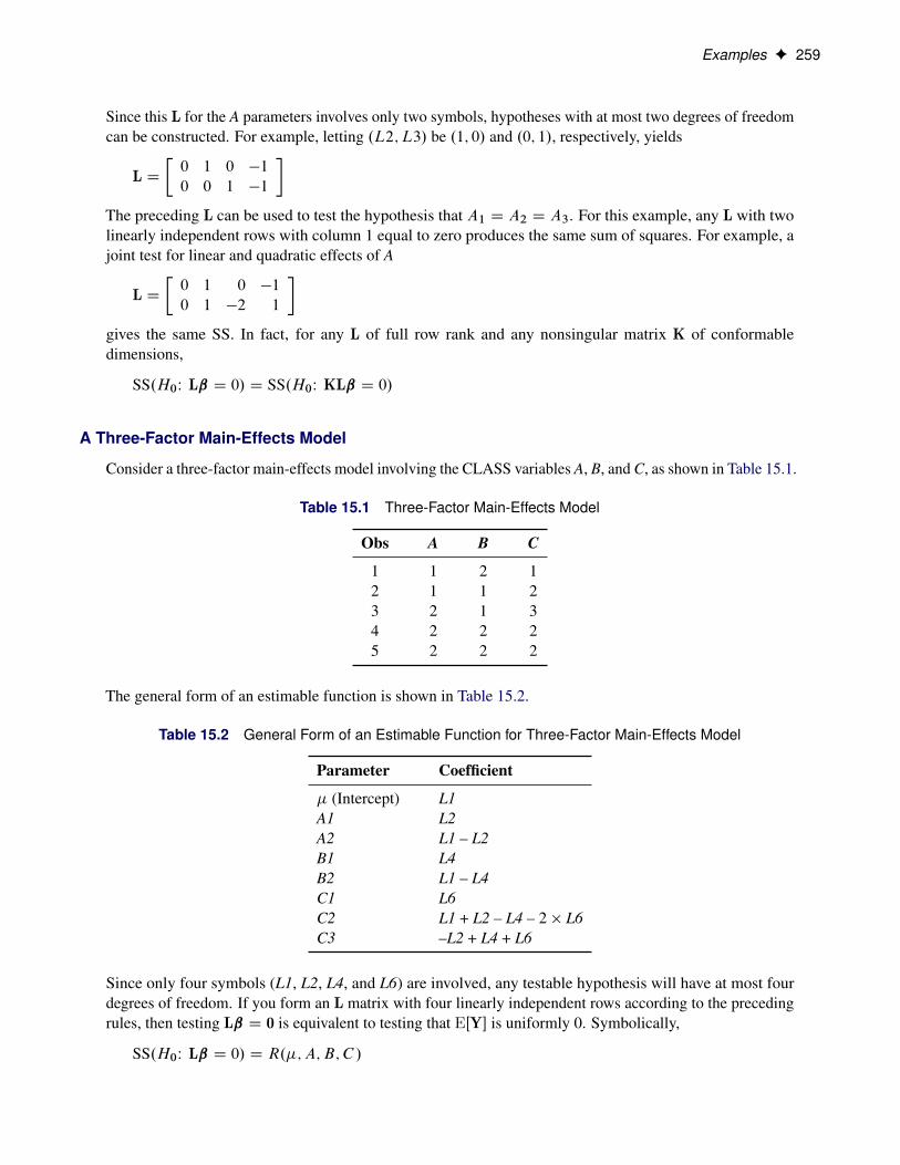
Consider a three-factor main-effects model involving the CLASS variables A, B, and C, as shown in Table 15.1.

Table 15.1 Three-Factor Main-Effects Model

Obs A B C

1 1 2 12 1 1 23 2 1 34 2 2 25 2 2 2

The general form of an estimable function is shown in Table 15.2.

Table 15.2 General Form of an Estimable Function for Three-Factor Main-Effects Model

Parameter Coefficient

� (Intercept) L1A1 L2A2 L1 – L2B1 L4B2 L1 – L4C1 L6C2 L1 + L2 – L4 – 2 � L6C3 –L2 + L4 + L6

Since only four symbols (L1, L2, L4, and L6) are involved, any testable hypothesis will have at most fourdegrees of freedom. If you form an L matrix with four linearly independent rows according to the precedingrules, then testing Lˇ D 0 is equivalent to testing that EŒY� is uniformly 0. Symbolically,

SS.H0W Lˇ D 0/ D R.�;A;B; C /


In a main-effects model, the usual hypothesis of interest for a main effect is the equality of all the parameters.In this example, it is not possible to unambiguously test such a hypothesis because of confounding: any testfor the equality of the parameters for any one of A, B, or C will necessarily involve the parameters for theother two effects. One way to proceed is to construct a maximum rank hypothesis (MRH) involving only theparameters of the main effect in question. This can be done using the general form of estimable functions.Note the following:

• To get an MRH involving only the parameters of A, the coefficients of L associated with �, B1, B2,C1, C2, and C3 must be equated to zero. Starting at the top of the general form, let L1 = 0, then L4 =0, then L6 = 0. If C2 and C3 are not to be involved, then L2 must also be zero. Thus, A1 – A2 is notestimable; that is, the MRH involving only the A parameters has zero rank and R.A j �;B;C / D 0.

• To obtain the MRH involving only the B parameters, let L1 = L2 = L6 = 0. But then to removeC2 and C3 from the comparison, L4 must also be set to 0. Thus, B1 – B2 is not estimable andR.B j �;A;C / D 0.

• To obtain the MRH involving only the C parameters, let L1 = L2 = L4 =0. Thus, the MRH involvingonly C parameters is

C1 � 2 � C2 C C3 D K (for any K)

or any multiple of the left-hand side equal to K. Furthermore,

SS.H0W C1 � 2 � C2 C C3 D 0/ D R.C j �;A;B/

A Multiple Regression Model

Suppose

EŒY � D ˇ0 C ˇ1x1 C ˇ2x2 C ˇ3x3

where the X0X matrix has full rank. The general form of estimable functions is as shown in Table 15.3.

Table 15.3 General Form of Estimable Functions for a Multiple Regression Model When X0X Matrix Is ofFull Rank


ˇ0 L1ˇ1 L2ˇ2 L3ˇ3 L4

For example, to test the hypothesis that ˇ2 D 0, let L1 = L2 = L4 = 0 and let L3 = 1. Then SS.Lˇ D 0/ DR.ˇ2 j ˇ0; ˇ1; ˇ3/. In this full-rank case, all parameters, as well as any linear combination of parameters,are estimable.

Suppose, however, that X3 D 2x1 C 3x2. The general form of estimable functions is shown in Table 15.4.

Estimable Functions F 261

Table 15.4 General Form of Estimable Functions for a Multiple Regression Model When X0X Matrix IsNot of Full Rank


ˇ0 L1ˇ1 L2ˇ2 L3ˇ3 2 � L2 C 3 � L3

For this example, it is possible to test H0Wˇ0 D 0. However, ˇ1, ˇ2, and ˇ3 are not jointly estimable; that is,

R.ˇ1 j ˇ0; ˇ2; ˇ3/ D 0

R.ˇ2 j ˇ0; ˇ1; ˇ3/ D 0

R.ˇ3 j ˇ0; ˇ1; ˇ2/ D 0

Estimable Functions

Type I SS and Estimable FunctionsIn PROC GLM, the Type I SS and the associated hypotheses they test are byproducts of the modified sweepoperator used to compute a generalized g2-inverse of X0X and a solution to the normal equations. For themodel EŒY � D x1ˇ1 C x2ˇ2 C x3ˇ3, the Type I SS for each effect are as follows:

Effect Type I SS

x1 R.ˇ1/

x2 R.ˇ2 j ˇ1/

x3 R.ˇ3 j ˇ1; ˇ2/

Note that some other SAS/STAT procedures compute Type I hypotheses by sweeping X0X (for example,PROC MIXED and PROC GLIMMIX), but their test statistics are not necessarily equivalent to the results ofusing those procedures to fit models that contain successively more effects.

The Type I SS are model-order dependent; each effect is adjusted only for the preceding effects in themodel.

There are numerous ways to obtain a Type I hypothesis matrix L for each effect. One way is to form the X0Xmatrix and then reduce X0X to an upper triangular matrix by row operations, skipping over any rows with azero diagonal. The nonzero rows of the resulting matrix associated with x1 provide an L such that

SS.H0W Lˇ D 0/ D R.ˇ1/


The nonzero rows of the resulting matrix associated with x2 provide an L such that

SS.H0W Lˇ D 0/ D R.ˇ2 j ˇ1/

The last set of nonzero rows (associated with x3) provide an L such that

SS.H0W Lˇ D 0/ D R.ˇ3 j ˇ1; ˇ2/

Another more formalized representation of Type I generating sets for x1, x2, and x3, respectively, is

G1 D . X01X1 j X01X2 j X01X3 /

G2 D . 0 j X02M1X2 j X02M1X3 /

G3 D . 0 j 0 j X03M2X3 /

where

M1 D I � X1.X01X1/�X01

and

M2 DM1 �M1X2.X02M1X2/�X02M1

Using the Type I generating set G2 (for example), if an L is formed from linear combinations of the rows ofG2 such that L is of full row rank and of the same row rank as G2, then SS.H0W Lˇ D 0/ D R.ˇ2 j ˇ1/.

In the GLM procedure, the Type I estimable functions displayed symbolically when the E1 option is requestedare

G�1 D .X01X1/�G1

G�2 D .X02M1X2/�G2

G�3 D .X03M2X3/�G3

As can be seen from the nature of the generating sets G1, G2, and G3, only the Type I estimable functionsfor ˇ3 are guaranteed not to involve the ˇ1 and ˇ2 parameters. The Type I hypothesis for ˇ2 can (and oftendoes) involve ˇ3 parameters, and likewise the Type I hypothesis for ˇ1 often involves ˇ2 and ˇ3 parameters.

There are, however, a number of models for which the Type I hypotheses are considered appropriate. Theseare as follows:

• balanced ANOVA models specified in proper sequence (that is, interactions do not precede main effectsin the MODEL statement and so forth)

• purely nested models (specified in the proper sequence)

• polynomial regression models (in the proper sequence)

Type II SS and Estimable Functions F 263

Type II SS and Estimable FunctionsFor main-effects models and regression models, the general form of estimable functions can be manipulatedto provide tests of hypotheses involving only the parameters of the effect in question. The same result canalso be obtained by entering each effect in turn as the last effect in the model and obtaining the Type I SS forthat effect. These are the Type II SS. Using a modified reversible sweep operator, it is possible to obtain theType II SS without actually refitting the model.

Thus, the Type II SS correspond to the R notation in which each effect is adjusted for all other appro-priate effects. For a regression model such as

EŒY � D x1ˇ1 C x2ˇ2 C x3ˇ3

the Type II SS correspond to

Effect Type II SS

x1 R.ˇ1 j ˇ2; ˇ3/

x2 R.ˇ2 j ˇ1; ˇ3/

x3 R.ˇ3 j ˇ1; ˇ2/

For a main-effects model (A, B, and C as classification variables), the Type II SS correspond to

Effect Type II SS

A R.A j B;C /

B R.B j A;C /

C R.C j A;B/

As the discussion in the section “A Three-Factor Main-Effects Model” on page 259 indicates, for regressionand main-effects models the Type II SS provide an MRH for each effect that does not involve the parametersof the other effects.

In order to see what effects are appropriate to adjust for in computing Type II estimable functions, note thatfor models involving interactions and nested effects, in the absence of a priori parametric restrictions, it isnot possible to obtain a test of a hypothesis for a main effect free of parameters of higher-level interactionseffects with which the main effect is involved. It is reasonable to assume, then, that any test of a hypothesisconcerning an effect should involve the parameters of that effect and only those other parameters with whichthat effect is involved. The concept of effect containment helps to define this involvement.

Contained EffectGiven two effects F1 and F2, F1 is said to be contained in F2 provided that the following two conditions aremet:

• Both effects involve the same continuous variables (if any).

• F2 has more CLASS variables than F1 does, and if F1 has CLASS variables, they all appear in F2.


Note that the intercept effect � is contained in all pure CLASS effects, but it is not contained in any effectinvolving a continuous variable. No effect is contained by �.

Type II, Type III, and Type IV estimable functions rely on this definition, and they all have one thing incommon: the estimable functions involving an effect F1 also involve the parameters of all effects that containF1, and they do not involve the parameters of effects that do not contain F1 (other than F1).

Hypothesis Matrix for Type II Estimable FunctionsThe Type II estimable functions for an effect F1 have an L (before reduction to full row rank) of the followingform:

• All columns of L associated with effects not containing F1 (except F1) are zero.

• The submatrix of L associated with effect F1 is .X01MX1/�.X01MX1/.

• Each of the remaining submatrices of L associated with an effect F2 that contains F1 is.X01MX1/

�.X01MX2/.

In these submatrices,

X0 D the columns of X whose associated effects do not contain F1

X1 D the columns of X associated with F1

X2 D the columns of X associated with an F2 effect that containsF1

M D I � X0.X00X0/�X00

For the model

class A B;model Y = A B A*B;


R.A j �;B/; R.B j �;A/; R.A � B j �;A;B/

for effects A, B, and A * B, respectively. For the model

class A B C;model Y = A B(A) C(A B);


R.A j �/; R.B.A/ j �;A/; R.C.AB/ j �;A;B.A//

for effects A, B.A/ and C.AB/, respectively. For the model

model Y = x x*x;

Type II SS and Estimable Functions F 265


R.X j �;X �X/ and R.X �X j �;X/

for x and x � x, respectively.

Note that, as in the situation for Type I tests, PROC MIXED and PROC GLIMMIX compute Type I hypothesesby sweeping X0X, but their test statistics are not necessarily equivalent to the results of sequentially fittingwith those procedures models that contain successively more effects; while PROC TRANSREG computestests labeled as being Type II by leaving out each effect in turn, but the specific linear hypotheses associatedwith these tests might not be precisely the same as the ones derived from successively sweeping X0X.

Example of Type II Estimable Functions

For a 2 � 2 factorial with w observations per cell, the general form of estimable functions is shown inTable 15.5. Any nonzero values for L2, L4, and L6 can be used to construct L vectors for computing the TypeII SS for A, B, and A * B, respectively.

Table 15.5 General Form of Estimable Functions for 2 � 2 Factorial

Effect Coefficient

� L1A1 L2A2 L1 – L2B1 L4B2 L1 – L4AB11 L6AB12 L2 – L6AB21 L4 – L6AB22 L1 – L2 – L4 + L6

For a balanced 2 � 2 factorial with the same number of observations in every cell, the Type II estimablefunctions are shown in Table 15.6.

Table 15.6 Type II Estimable Functions for Balanced 2 � 2 Factorial

Coefficients for EffectEffect A B A * B

� 0 0 0A1 L2 0 0A2 –L2 0 0B1 0 L4 0B2 0 –L4 0AB11 0.5 � L2 0.5 � L4 L6AB12 0.5 � L2 –0.5 � L4 –L6AB21 –0.5 � L2 0.5 � L4 –L6AB22 –0.5 � L2 –0.5 � L4 L6


Now consider an unbalanced 2 � 2 factorial with two observations in every cell except the AB22 cell, whichcontains only one observation. The general form of estimable functions is the same as if it were balanced,since the same effects are still estimable. However, the Type II estimable functions for A and B are not thesame as they were for the balanced design. The Type II estimable functions for this unbalanced 2� 2 factorialare shown in Table 15.7.

Table 15.7 Type II Estimable Functions for Unbalanced 2 � 2 Factorial

Coefficients for EffectEffect A B A * B

� 0 0 0A1 L2 0 0A2 –L2 0 0B1 0 L4 0B2 0 –L4 0AB11 0.6 � L2 0.6 � L4 L6AB12 0.4 � L2 –0.6 � L4 –L6AB21 –0.6 � L2 0.4 � L4 –L6AB22 –0.4 � L2 –0.4 � L4 L6

By comparing the hypothesis being tested in the balanced case to the hypothesis being tested in the unbalancedcase for effects A and B, you can note that the Type II hypotheses for A and B are dependent on the cellfrequencies in the design. For unbalanced designs in which the cell frequencies are not proportional tothe background population, the Type II hypotheses for effects that are contained in other effects are ofquestionable value.

However, if an effect is not contained in any other effect, the Type II hypothesis for that effect is an MRHthat does not involve any parameters except those associated with the effect in question.

Thus, Type II SS are appropriate for the following models:

• any balanced model

• any main-effects model

• any pure regression model

• an effect not contained in any other effect (regardless of the model)

In addition to the preceding models, Type II SS are generally accepted by most statisticians for purely nestedmodels.

Type III and IV SS and Estimable FunctionsWhen an effect is contained in another effect, the Type II hypotheses for that effect are dependent on the cellfrequencies. The philosophy behind both the Type III and Type IV hypotheses is that the hypotheses testedfor any given effect should be the same for all designs with the same general form of estimable functions.

Type III and IV SS and Estimable Functions F 267

To demonstrate this concept, recall the hypotheses being tested by the Type II SS in the balanced 2�2 factorialshown in Table 15.6. Those hypotheses are precisely the ones that the Type III and Type IV hypothesesemploy for all 2�2 factorials that have at least one observation per cell. The Type III and Type IV hypothesesfor a design without missing cells usually differ from the hypothesis employed for the same design withmissing cells since the general form of estimable functions usually differs.

Many SAS/STAT procedures can perform tests of Type III hypotheses, but only PROC GLM offers Type IVtests as well.

Type III Estimable Functions

Type III hypotheses are constructed by working directly with the general form of estimable functions. Thefollowing steps are used to construct a hypothesis for an effect F1:

1. For every effect in the model except F1 and those effects that contain F1, equate the coefficients in thegeneral form of estimable functions to zero.

If F1 is not contained in any other effect, this step defines the Type III hypothesis (as well as the TypeII and Type IV hypotheses). If F1 is contained in other effects, go on to step 2. (See the section “TypeII SS and Estimable Functions” on page 263 for a definition of when effect F1 is contained in anothereffect.)

2. If necessary, equate new symbols to compound expressions in the F1 block in order to obtain thesimplest form for the F1 coefficients.

3. Equate all symbolic coefficients outside the F1 block to a linear function of the symbols in the F1block in order to make the F1 hypothesis orthogonal to hypotheses associated with effects that containF1.

By once again observing the Type II hypotheses being tested in the balanced 2 � 2 factorial, it is possible toverify that the A and A * B hypotheses are orthogonal and also that the B and A * B hypotheses are orthogonal.This principle of orthogonality between an effect and any effect that contains it holds for all balanced designs.Thus, construction of Type III hypotheses for any design is a logical extension of a process that is used forbalanced designs.

The Type III hypotheses are precisely the hypotheses being tested by programs that reparameterize using theusual assumptions (for example, constraining all parameters for an effect to sum to zero). When no missingcells exist in a factorial model, Type III SS coincide with Yates’ weighted squares-of-means technique. Whencells are missing in factorial models, the Type III SS coincide with those discussed in Harvey (1960) andHenderson (1953).

The following discussion illustrates the construction of Type III estimable functions for a 2 � 2 factorial withno missing cells.

To obtain the A * B interaction hypothesis, start with the general form and equate the coefficients for effects�, A, and B to zero, as shown in Table 15.8.


Table 15.8 Type III Hypothesis for A * B Interaction

Effect General Form L1 = L2 = L4 = 0

� L1 0A1 L2 0A2 L1 – L2 0B1 L4 0B2 L1 – L4 0AB11 L6 L6AB12 L2 – L6 –L6AB21 L4 – L6 –L6AB22 L1 – L2 – L4 + L6 L6

The last column in Table 15.8 represents the form of the MRH for A * B.

To obtain the Type III hypothesis for A, first start with the general form and equate the coefficients for effects� and B to zero (let L1 = L4 = 0). Next let L6 = K � L2, and find the value of K that makes the A hypothesisorthogonal to the A * B hypothesis. In this case, K = 0.5. Each of these steps is shown in Table 15.9.

In Table 15.9, the fourth column (under L6 = K � L2) represents the form of all estimable functions notinvolving �, B1, or B2. The prime difference between the Type II and Type III hypotheses for A is the way Kis determined. Type II chooses K as a function of the cell frequencies, whereas Type III chooses K such thatthe estimable functions for A are orthogonal to the estimable functions for A * B.

Table 15.9 Type III Hypothesis for A

Effect General Form L1 = L4 = 0 L6 = K � L2 K= 0.5

� L1 0 0 0A1 L2 L2 L2 L2A2 L1 – L2 –L2 –L2 –L2B1 L4 0 0 0B2 L1 – L4 0 0 0AB11 L6 L6 K � L2 0.5 � L2AB12 L2 – L6 L2 – L6 (1 – K) � L2 0.5 � L2AB21 L4 – L6 –L6 –K � L2 –0.5 � L2AB22 L1 – L2 – L4 + L6 –L2 + L6 –(1 – K) � L2 –0.5 � L2

An example of Type III estimable functions in a 3 � 3 factorial with unequal cell frequencies and missingdiagonals is given in Table 15.10 (N1 through N6 represent the nonzero cell frequencies).

Table 15.10 3 � 3 Factorial Design with Unequal Cell Frequencies and Missing Diagonals

B1 2 3

1 N1 N2

A 2 N3 N4

3 N5 N6

Type III and IV SS and Estimable Functions F 269

For any nonzero values of N1 through N6, the Type III estimable functions for each effect are shown inTable 15.11.

Table 15.11 Type III Estimable Functions for 3 � 3 Factorial Design with Unequal Cell Frequencies andMissing Diagonals

Effect A B A * B

� 0 0 0A1 L2 0 0A2 L3 0 0A3 –L2 – L3 0 0B1 0 L5 0B2 0 L6 0B3 0 –L5 – L6 0AB12 0.667 � L2 + 0.333 � L3 0.333 � L5 + 0.667 � L6 L8AB13 0.333 � L2 – 0.333 � L3 –0.333 � L5 – 0.667 � L6 –L8AB21 0.333 � L2 + 0.667 � L3 0.667 � L5 + 0.333 � L6 –L8AB23 –0.333 � L2 + 0.333 � L3 –0.667 � L5 – 0.333 � L6 L8AB31 –0.333 � L2 – 0.667 � L3 0.333 � L5 – 0.333 � L6 L8AB32 –0.667 � L2 – 0.333 � L3 –0.333 � L5 + 0.333 � L6 –L8

Type IV Estimable Functions

By once again looking at the Type II hypotheses being tested in the balanced 2 � 2 factorial (see Table 15.6),you can see another characteristic of the hypotheses employed for balanced designs: the coefficients oflower-order effects are averaged across each higher-level effect involving the same subscripts. For example,in the A hypothesis, the coefficients of AB11 and AB12 are equal to one-half the coefficient of A1, and thecoefficients of AB21 and AB22 are equal to one-half the coefficient of A2. With this in mind, the basicconcept used to construct Type IV hypotheses is that the coefficients of any effect, say F1, are distributedequitably across higher-level effects that contain F1. When missing cells occur, this same general philosophyis adhered to, but care must be taken in the way the distributive concept is applied.

Construction of Type IV hypotheses begins as does the construction of the Type III hypotheses. That is, foran effect F1, equate to zero all coefficients in the general form that do not belong to F1 or to any other effectcontaining F1. If F1 is not contained in any other effect, then the Type IV hypothesis (and Type II and III)has been found. If F1 is contained in other effects, then simplify, if necessary, the coefficients associatedwith F1 so that they are all free coefficients or functions of other free coefficients in the F1 block.

To illustrate the method of resolving the free coefficients outside the F1 block, suppose that you are interestedin the estimable functions for an effect A and that A is contained in AB, AC, and ABC. (In other words, themain effects in the model are A, B, and C.)

With missing cells, the coefficients of intermediate effects (here they are AB and AC) do not always havean equal distribution of the lower-order coefficients, so the coefficients of the highest-order effects aredetermined first (here it is ABC). Once the highest-order coefficients are determined, the coefficients ofintermediate effects are automatically determined.

The following process is performed for each free coefficient of A in turn. The resulting symbolic vectors arethen added together to give the Type IV estimable functions for A.


1. Select a free coefficient of A, and set all other free coefficients of A to zero.

2. If any of the levels of A have zero as a coefficient, equate all of the coefficients of higher-level effectsinvolving that level of A to zero. This step alone usually resolves most of the free coefficients remaining.

3. Check to see if any higher-level coefficients are now zero when the coefficient of the associated levelof A is not zero. If this situation occurs, the Type IV estimable functions for A are not unique.

4. For each level of A in turn, if the A coefficient for that level is nonzero, count the number of timesthat level occurs in the higher-level effect. Then equate each of the higher-level coefficients to thecoefficient of that level of A divided by the count.

An example of a 3� 3 factorial with four missing cells (N1 through N5 represent positive cell frequencies) isshown in Table 15.12.

Table 15.12 3 � 3 Factorial Design with Four Missing Cells

B1 2 3

1 N1 N2

A 2 N3 N4

3 N5

The Type IV estimable functions are shown in Table 15.13.

Table 15.13 Type IV Estimable Functions for 3 � 3 Factorial Design with Four Missing Cells

Effect A B A * B

� 0 0 0A1 –L3 0 0A2 L3 0 0A3 0 0 0B1 0 L5 0B2 0 –L5 0B3 0 0 0AB11 –0.5 � L3 0.5 � L5 L8AB12 –0.5 � L3 –0.5 � L5 –L8AB21 0.5 � L3 0.5 � L5 –L8AB22 0.5 � L3 –0.5 � L5 L8AB33 0 0 0

A Comparison of Type III and Type IV Hypotheses

For the vast majority of designs, Type III and Type IV hypotheses for a given effect are the same. Specifically,they are the same for any effect F1 that is not contained in other effects for any design (with or withoutmissing cells). For factorial designs with no missing cells, the Type III and Type IV hypotheses coincidefor all effects. When there are missing cells, the hypotheses can differ. By using the GLM procedure, you

References F 271

can study the differences in the hypotheses and then decide on the appropriateness of the hypotheses for aparticular model.

The Type III hypotheses for three-factor and higher completely nested designs with unequal Ns in the lowestlevel differ from the Type II hypotheses; however, the Type IV hypotheses do correspond to the Type IIhypotheses in this case.

When missing cells occur in a design, the Type IV hypotheses might not be unique. If this occurs in PROCGLM, you are notified, and you might need to consider defining your own specific comparisons.

References

Freund, R. J., Littell, R. C., and Spector, P. C. (1991), SAS System for Linear Models, Cary, NC: SAS InstituteInc.

Goodnight, J. H. (1978), Tests of Hypotheses in Fixed-Effects Linear Models, Technical Report R-101, SASInstitute Inc., Cary, NC.

Goodnight, J. H. (1979), “A Tutorial on the Sweep Operator,” American Statistician, 33, 149–158.

Harvey, W. R. (1960), Least-Squares Analysis of Data with Unequal Subclass Frequencies, Technical ReportARS 20-8, U.S. Department of Agriculture, Agriculture Research Service.

Henderson, C. R. (1953), “Estimation of Variance and Covariance Components,” Biometrics, 9, 226–252.

Milliken, G. A. and Johnson, D. E. (1984), Designed Experiments, Analysis of Messy Data, Belmont, CA:Lifetime Learning Publications.

the four types of estimable functions - sas...introduction to reduction notation f 257 since all...

Documents