the formal posterior of a standard flat prior in manova is incoherent

J. ltal. Statist. Soc. (1995) 2, pp. 251-270

THE FORMAL POSTERIOR OF A STANDARD FLAT PRIOR IN MANOVA IS INCOHERENT*

M o r r i s L . E a t o n * *

W i l l i a m D . S u d d e r t h University of Minnesota

Summary

A standard improper prior for the parameters of a MANOVA model is shown to yield an inference that. is incoherent in the sense of Heath and Sudderth. The proof of incoherence is based on the fact that the formal Bayes estimate, say 60, of the covariance matrix based on the improper prior and a certain bounded loss function is uniformly inadmissible in that there is another estimator 6t and an e > 0 such that the risk functions satisfy R(61, Y,) <~ R(6o, Y,) - e for all values of the covariance matrix 2,. The estimator 6/is formal Bayes for an alternative improper prior which leads to a coherent inference.

Keywords: coherent inference, improper prior, invariant estimation, uniform inadmissibility, Haar measure.

O. Introduction

Let 0-g be the set of possible values for a data variable Y whose probabil i ty distribution P(.[O) depends on a state of nature 0 with possible values in a pa rame te r space O. By an inference we mean a mapping R which assigns to each y ~ ~ a probabili ty distribution R(. ly) on O. An inference might correspond to a posterior distribution, a system of confidence regions, or even a fiducial distribution. The use of inference in this sense appeared earlier in Ea ton (1982) and Lane and Sudderth (1983).

An inference R can be given an interpretat ion in economic or gambling terminology as a rule for posting odds on the true state of nature t~ after observing Y. The inference is called coherent by Hea th and Sudderth (1978) if it is impossible for a gambler to devise a finite system of bets that attains an expected payoff greater than some positive constant for every O. The precise

* Research supported by National Science Foundation grants DMS-89-22607 (for Eaton) and DMS-9123358 (for Sudderth). ** Address for correspondence: M. L. Eaton, Dept. of Theoretical Statistics, 270 Vincent Hall, University of Minnesota, 206 Church Street S.E., Minneapolis, MN 55455, U.S.A.

251

M. L. E A T O N �9 W . D . S U D D E R T H

definition is given in w 4 and was inspired by the ideas of de Finetti and a paper of Freedman and Purves (1969).

An interesting alternative notion of coherence for inferences was defined by Regazzini (1987). This definition of Regazzini was compared and con- trasted with that of Heath and Sudderth in the papers of Berti, Regazzini, and Rigo (1991) and Berti and Rigo (1994). In this paper we will use the term ,<coherence~ in the sense defined by Heath and Sudderth.

An inference R that corresponds to the posterior of a proper prior can easily be shown to be coherent. However, the formal posterior of an improper prior may or may not be coherent (Heath and Sudderth (1978, 1989)). Such formal Bayes inferences are of interest because they are often used by Bayesians and also because many widely-used non-Bayesian inferences agree with some formal Bayes inference.

In this paper our main object is to study the formal posterior O of the standard ,,flat~ prior ~ for the MANOVA model introduced in w 1 below. The improper prior ~ arises naturally in two ways. First, as is explained in w 1, the MANOVA model is invariant under the left action of a certain natural group G and ~ is the prior induced by the right Haar measure on G. Second, as Box and Tiao (1973) explain, ~ is the <~noninformative~ prior derived from a criterion of Jeffreys. It turns out that the inference Q si coherent in the univariate case (Theorem 4.3) and is incoherent in dimensions greater than one (Theorem 4.2).

Because the group G is amenable in the univariate case, the coherence of Q follows easily from results of Heath and Sudderth (1978) and Wetzel (1993). Most of the paper is devoted to the proof of incoherence in higher dimensions where G is not amenable. Our inadmissibility results parallel those in James and Stein (1960), although our model of proof is different. They considered the problem of estimating the covariance _r for a certain unbounded, G-invariant loss function L. In w 2 we consider the same problem for the bounded, G-invariant loss function l = 1 - exp(-L). The best G-invariant estimator tG is calculated and shown to be formal Bayes for the improper prior ~. In w 3 we consider a proper subgroup H of G and calculate the best H-invariant estimator tH which is formal Bayes for the improper prior 0r corresponding to a right Haar measure on H. It is shown that tn uniformly dominates tG and is the minimax rule (Theorem 3.4). It is then easy to deduce the incoherence of Q in w 4 where it is also shown that the formal Bayes inference Q from the improper prior ~'r is coherent in all dimensions.

Perhaps the first examples of incoherent inferences from uniform priors are due to Stone (1976). Under mild measurability assumptions, Stone's notion of ,,strong inconsistency~, is essentially equivalent to incoherence (Lane

252

FLAT PRIOR IN MANOVA

and Sudderth (1983), Berti and Rigo (1994)). Stone's interesting examples also illustrate the role played by nonamenable groups. Our example may be the first in which a standard statistical inference is seen to be incoherent.

It is easier for the formal posterior of an improper prior to be coherent in the sense of Regazzini (1987). Indeed, all of the specific inferences considered in this paper are coherent in his sense as follows f rom Proposit ion 4.2 in Berti and Rigo (1994).

1. Invariance of the Model

Here we consider a M A N O V A model in canonical form and describe the classical group invariance of the model. More precisely, suppose a data matrix Y: n x p has a multivariate normal distribution with a mean matrix

%Y= (B), B: k x p (1.1)

and covariance given by

Cov(Y) = I,, @ 2" (1.2)

where Z is an unknown p • p positive definite matrix. Thus the matrix Y has independent rows each with covariance matrix Z, and the mean matrix of Y is assumed to have the form (1.1) where B is an unknown k • p real matrix. This we write as

(1.3)

In what follows, it is convenient to partition Y as

I"1) (1.4) Y = Y2

where I,'1 is k x p and Y2 is m x p with m = n - k. It is assumed that m ~> p. For future use, set

S = Y'2Y2 (1.5)

so S has a W(,,Y, p, m) distribution - the Wishart distribution with parameters 2, p and m degrees of freedom.

253

M. L. E A T O N �9 W . D. S U D D E R T H

Let G be the group whose elements are

g = (A, c) (1.6)

where 3 is a p x p nonsingular matrix and c is a k x p real matrix. T h e group operation is

(AI, cl) (32, r = (A1A2, cl + c2A'I) (1.7)

where the prime denotes transpose. Then G acts on the sample space via

+(0 ) It is easy to check this is a left action when group composition is (1.7). Furth- ermore, the induced left action of G on the parameter point 0 = (~, B) is

(27, B)---~ ( A Z A ' , B A ' + c). (1.9)

With these two group actions, it is clear that the model specified by (1.3) is invariant.

In our discussion to follow, we also need to consider a subgroup H of G. Elements of the subgroup H are

h = (t, c) (1.10)

where again c is a k x p real matrix, but t is a p x p lower triangular matrix whose diagonal elements are positive. Thus, H acts on the sample space and the parametric space via (1.8) and (1.9) respectively and the model (1.3) is invariant. The following proportion is well-known.

Proposition 1.1. The group H acts transitively on the parameter space - that is, given any parameter (27, B) there exists an h = (t, c) in H such tha t t$t ' = Ip and Bt ' + c = O.

Proof. That a t exists (and is unique) follows from Eaton (1983, p. 162). Next pick c = - B t ' . o

Since H acts transitively on the parameter space, so does the bigger group G.

254


2. A G-invariant estimation problem

Invariant estimation of the covariance matrix Z was discussed in James and Stein (1960). In the decision theoretic formulation of this problem, the action space is Sf~-, the space o f p x p positive definite matrices, and the loss function used by James and Stein was

L(a, ~) = tr(aZ - z ) - log d e t ( a ~ - t ) - p . (2.1)

Here , tr denotes the trace, and a is an element of b~ The action of the group G on 5~ - is

a ~ A a A ' . (2.2)

The invariance of L is easily checked. Observe that L(a, Z) is just a function of the eigenvalues of aZ --z (which are all positive), say )~1 . . . . . ~.p. It is easily checked that

P

L(a, Z) = ~, (Ai - log ~.i - 1). (2.3) i=1

The motivation of this loss function is that the function x ~ x - log x - 1 is convex on (0, oo), has a unique minimum of 0 at x = 1, and increases to ao as x approaches 0 or oo. Thus L(a, Z) can be thought of as a measure of how far the eigenvalues of aZ --1 ae from (1, 1, ..., 1).

For our purposes, (2.3) is not suitable because it is unbounded. The basic results of Heath and Sudderth (1978) concerning extended admissibility apply only to bounded loss functions. The loss function considered in this paper is

l(a, Z) = 1 - e x p [ - L ( a , Z)] (2.4)

where L is given in (2.3). Obviously t is invariant and bounded. Using this loss function we are able to calculate the best G and H invariant estimators of Z.

The method used to calculate the best invariant estimators is based on a result due to Stein. The form of Stein's result used here is discussed in Eaton (1989, pp. 84-94). To describe the method, consider the group G and let Vr denote a right Haar measure on G. Because G is transitive on the parameter

255


space O = {(27, B) I 27 ~ 5f~, B : k x p}, vr induces an improper prior distribution ~ on O via the equation

fof(O) ~(dO)-- fo f(gOo) v,(dg) (2.5)

where 19o is a fixed point in O. That is, equation (2.5) is to hold for all non- negative measurable functions fdefined on O. It is easy to check that a right Haar measure on G is

v~(dg) = v~(dA, dC) = d c - dA iAiP (2.6)

where dc and dA denote Lebesgue measure. For convenience, pick O0 = (Ip, 0) cO. Now, standard results from the theory of Haar measure show that there is a constant k e (0, o0) such that the measure

~(dO) = ~(d,Y,, dB) = k d B - - d27

(2.7)

satisfies (2.5). Using the measure ~(dtg) as an improper prior distribution, Stein's result asserts that in the case at hand, a best invariant estimator is found by minimizing

~p(a) = f~e(a, ~) p(yla) ~(dO) (2.8)

where y is a fixed sample point and p(ylO) is the density function of the data (density with respect to Lebesgue) specified by (1.3). The minimizer, which we find below, say dr(y), is then the best invariant estimator of 27 relative to the loss function (2.4). The transitivity of G on O is a crucial ingredient in Stein's result. It implies that all invariant decision rules have constant risk, so it then makes sense to talk about a ~best,, invariant rule. The above prescrip- tion shows how to find the best invariant rule using the formal Bayes method - namely, by minimizing the posterior risk (2.8).

We now turn to the minimization of (2.8).

Theorem 2.1. Consider the measure ~ given by (2.7), the loss function given by (2.4) and the density of Y specified by the model (1.3). Then the function ~p defined by (2.8) is minimzed at

1 a(y) = - - s (2.9)

m

256


where m = n - k and s (as a function of y) is defined in (1.5).

R e m a r k . Since 27 is assumed to be non-singular, the data matrix Y has rank p with probability one and S is positive definite with probability one. In the s tatement of Theorem 2.1 and what follows, we take s to be positive definite.

Q

Proof . In what follows, we use the symbol gal, to mean that two functions of a ~ 9~ - are equal up to a positive constant (which can depend on y). The partitioning o f y : n • p into y, : k x p and Y2 : m x p is the same as the partitioning of Y in (1.4). The form of the loss function, of ~, and of the density p(y lO) shows that to minimize ~p(a), it is sufficient to maximize

W,(a) = f exp[-L(a, 27)] Ixl -"'2 (2.10)

[ 1 1 ] exp - -~- tr(yl - B ) Z --1 (Yt - B ) ' - ~ - tr s27 --1

Integrating out B and using the form of L yields

/ [ 1 tr(s+2a)X._l] dX v/ ,(a) alia I IXl - r '+e) /2exp - --~ iX[(p+~)/2

Setting ti = s - v 2 as - m and doing a bit of algebra gives

d27 d B

(2.11)

]a] i s + 2 a [ ( m + 2 ) / 2 "

~ , ( a ) d lal 1i+2dl ( m + 2 ) / 2 "

(2.12)

However , the right side of (2.12) can be written

P / 7 v, i=, (1 +2vi) (m+2)/2

(2.13)

where Vl . . . . , Vp are the eigenvalues of ti. Since the function v ~ v/(1 + 1

2v) ~ is uniquely maximized (over 0, oo) at v = - - , it follows that the m

right side of (2.12) is uniquely maximized at d = m - l i p . Therefore ~p/ is uniquely maximized at a = ~(y) = m - I s . This completes the proof. []

Summarizing the above discussion gives

257

M. L. EATON �9 W . D. S U D D E R T H

Theorem 2.2. Given the model (1.3) and the loss function (2.4), the best G-invariant estimator of 27 is

ta(Y) = m - i S (2.14)

where S is defined in (1.5). This best invariant estimator is a formal Bayes rule when the improper prior is ~(dO) given by (2.7). In other words, ta(y) is the minimizer of the posterior risk

a -->/t(a, 27) q(Oly) ~(dO). (2.15)

Here q(~ is the posterior density (with respect to ~) given by

q(Oly) - P(Yl O) (2.16) m(y)

where

m(y) =/p(y lO) ~(dO). (2.17)

Theorem 2.3. The risk of the best G-invariant estimator tc in (2.14) is

ro = 1 ePw(m'P) m-e w(m+2,p) (1 +2m-1) p~m+2)/2 (2.18)

where w(o, o) is the standard Wishart constant (see Eaton (1983, p. 175)).

Proof. Because tc has constant risk, its risk is

rc = %ag(tc(Y), Ip) (2.19)

where %0 denotes expectation under the model when B = 0 and 27 = Ip. Using the form of ~ and the fact that to(Y ) depends on Y only through S = II'27"2 allows us to write (2.19) as

(2.20)

/ [ ] 1 dS r G 1 -- ePm -p w(m, p) [S](m+2)/2exp - - ~ tr(1 + 2m-1)S ]S](p+t)/2.

Making a change of variable and using the definition of w(~ .) yields (2.18). []

258


3. A best H-invariant estimator

It was noted in Section 1 that H, as well as G, acts transitively on 8 . There- fore, the same argument used in Section 2 to find a best G-invafiant decision rule can be used here to find a best H-invafiant rule. Let G ~ denote the group of all p x p lower triangular matrices which have strictly positive diagonal elements. For each p • p positive definite Z, there exists a unique y in G~ such that

= yy'. (3.1)

Obviously, (3.1) defines a one-to-one onto map between 5~p and G~. Thus, we can parameterize our model with 77 = (y, fl) where y~ G ~ and B is a k • p real matrix. Recall that elements h e H are written as

h = (t, c), t ~ G ~ , c : k x p . (3.2)

In this new parametfization, H acts on the parameter space via

(y, B) ~ (ty, Bt' + c), (3.3)

and the model is invariant with the action (3.3) on 7/. Let P(YlY, B) be the density function (with respect to Lebesgue measure) for the model (1.3) in the new parameterization.

Let Qr denote a fight Haar measure on H. Note that the parameter space for the model is just H itself. With 7/0 = (Ip, 0), the analog of equation (2.5) simply induces the improper prior distribution Qr on the parameter space H. It is easy to check that a right Haar measure on H is

pr(dy, dB) = dB t2r(d'f) (3.4)

where I.tr(d'f) is a fight Haar measure on G~- given by

l~r(dy ) __ d)p ( 3 . 5 ) P

U ) / iPi - i+ l i=l

Here d y is Lebesgue measure on G~- and Y11 . . . . . ypp are the diagonal elements of y [see Eaton (1989, pp. 16-18) for a discussion of this]. Further , a left Haar measure on G~- is

259

M. L. EATON �9 W. D. SUDDERTH

#t (dy) = A ( y ) #r(dy) (3.6)

where A(o) is the modular function of G~ given by

P A(~/) = E l ~/iPi -2i+1. ( 3 . 7 )

i=l

In what follows the one-to-one onto correspondence between b~ - and G f plays a central role. For each u �9 SOp, let r denote the unique e lement of G ~ which satisfies

u = ~o(u) (q) (u) ) ' .

Thus, ~ is a function from S~ - to G~- which is bijection. Also no te that satisfies

cp(huh') = hop(u); u �9 SO~, h �9 G~-.

This follows from the uniqueness of cp(u). Given u �9 SO~-, cp(u) is of ten called the lower triangular square root of u (with the understanding that q~(u) �9 G~).

From Stein's results, a best H-invariant estimator of-Y" = yy' is calculated by finding the minimizer (over SOp) of

W2(a) = J e(a, r / ) P(YI~', B) Qr(dy, dB) ( 3 . 8 )

for each fixed y. Using the notation set in section 2, recall that

s = Y'2Ye (3.9)

is assumed to be positive definite (a set of measure zero in the sample space is being ignored). For notational convenience, let t = q~(s) so

s = tt', t �9 G~-. (3.10)

Theorem 3.1. Given s in (3.9), the unique element d = ~(y) E S~ which minimizes ~p2(~ in (3.8) is

d(y) = tDt ' (3.11)

where t is defined in (3.10) and D is a p x p diagonal matrix with diagonal elements

260

FLAT PRIOR IN M A N O V A

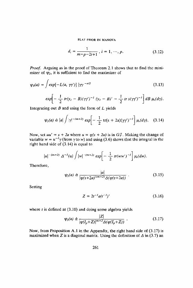
1 di - m + p -''-tztt l ' i = 1, . . . , p. (3.12)

Proof. Arguing as in the proof of Theorem 2.1 shows that to find the minimizer of ~P2, it is sufficient to find the maximizer of

~03(a) = / e x p [ - L ( a , yy')] - n ' 2 (3.13)

[ 1 exp - - ~ tr(yz - B)(y7') -1 (Yz - B) ' ~ tr s(gy') -1 dB l~r(dy).

2

Integrating out B and using the form of L yields

[_ 1 tr(s + 2a)(yy') -1] I~r(dg) (3.14) V23(a) d[al fill -(m§ exp - ~

Now, set uu' = s + 2a where u = qo(s + 2a) is in G~. Making the change of variable w = u - l y (from y to w) and using (3.6) shows that the integral in the right hand side of (3.14) is equal to

1 tr(ww,)_z] t~,(dw). lU[ -(m+2) A-l(u)/lwl-(m+2)exp[----~

Therefore,

Lal ~P3(a) d ] q)(s + 2a) I (''+2) A (cp(s + 2a)) (3.15)

Setting

Z = 2t-Za(t-z) ' (3.16)

where t is defined at (3.10) and doing some algebra yields

~03(a) dt Izl (3.17) i (ip§ z) l .2 zX(q (zp§ z)) �9

Now, from Proposition A.1 in the Appendix, the right hand side of (3.17) is maximized when Z is a diagonal matrix. Using the definition of A in (3.7) an

261


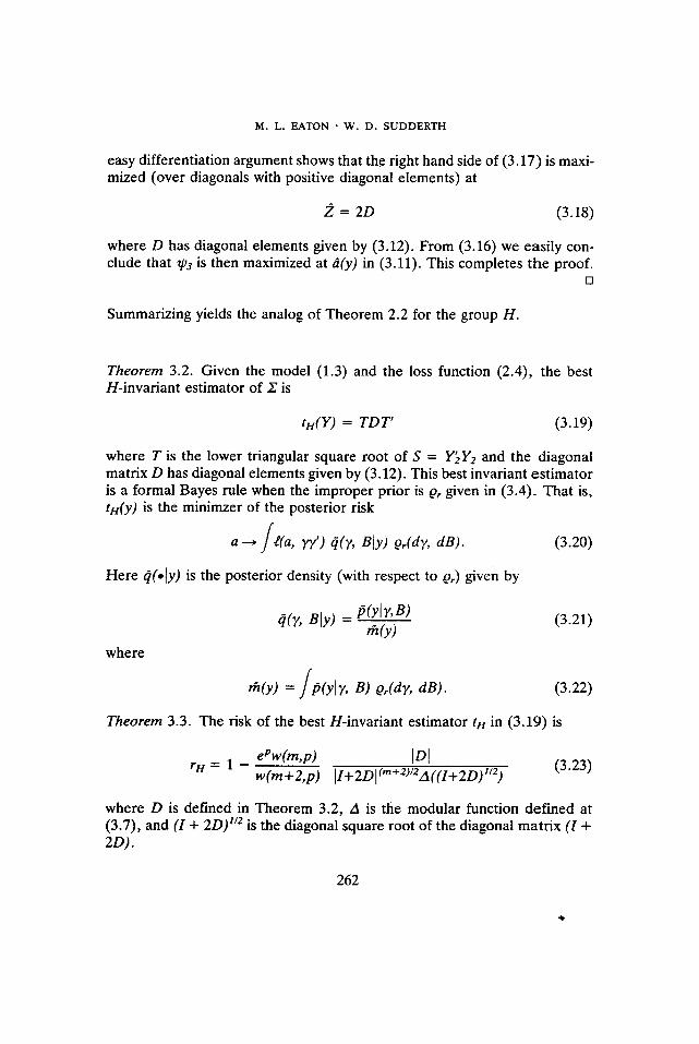
easy differentiation argument shows that th.e right hand side of (3.17) is maximized (over diagonals with positive diagonal elements) at

Z = 2D (3.18)

where D has diagonal elements given by (3.12). From (3.16) we easily conclude that ~P3 is then maximized at d(y) in (3.11). This completes the proof.

[]

Summarizing yields the analog of Theorem 2.2 for the group H.

Theorem 3.2. Given the model (1.3) and the loss function (2.4), the best H-invariant estimator of ~ is

t , ( Y ) = TDT' (3.19)

where T is the lower triangular square root of S = Y'2Y2 and the diagonal matrix D has diagonal elements given by (3.12). This best invariant estimator is a formal Bayes rule when the improper prior is Qr given in (3.4). That is, tn(y) is the minimzer of the posterior risk

a ~ / # ( a , yy') El(y, Bly) or(dY, dB). (3.20)

Here ~l(.[y) is the posterior density (with respect to @r) given by

where

~l(Y, Bly) - : (y]~' ,B) (3.21) rn(y)

rh(y) = f P(ylr, B) e,(dr, riB). (3.22)

Theorem 3.3. The risk of the best H-invariant estimator tH in (3.19) is

rn = 1 - ePw(m'P) [D] w(m+2,p) [I+2DICm+2mA((I+2D) 1/2)

(3.23)

where D is defined in Theorem 3.2, A is the modular function defined at (3.7), and (I + 2D) m is the diagonal square root of the diagonal matrix (I + 20).

262


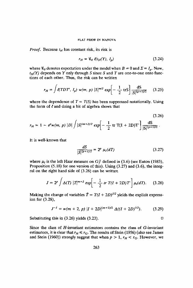
Proof . Because tH has constant risk, its risk is

rH = %0 r It,) (3.24)

where %0 denotes expectation under the model when B = 0 and ,S = It,. Now, tM(Y) depends on Y only through S since S and T are one-to-one onto functions of each other. Thus, the risk can be written

rn = r It,) w(m, p) IS[ m/2 exp - ~ trS [S1(p+1)/2

where the dependence of T = T(S) has been suppressed notationally. Using the form of I and doing a bit of algebra shows that

(3.26)

/ [ 1 tr T ( I + 2D)T'] dS rn = 1 - ePw(m, p) IOl Isl tin+2)/2 exp - -~- i s l ~ P + X ) ~ ,

It is well-known that

dS

Isl t,+, ,2 - - - 2 p I~,(dT) (3.27)

where /h is the left Haar measure on G~- defined in (3.6) (see Eaton (1983), Proposition (5.18) for one version of this). Using (3.27) and (3.6), the integral on the fight hand side of (3.26) can be written

/ [1 ] J = 2 p A (T ) 1~ m+eexp - - - ~ t r T ( I + 2 D ) T ' #r(dT). (3.28)

Making the change of variables T = T( I + 2D) 1/2 yields the explicit express- ion for (3.28),

j - 1 = w ( m + 2, p) 11 + 2D[ (m+2)/2 A ( ( I + 2D)i/z) . (3.29)

Substituting this in (3.26) yields (3.23). El

Since the class of H-invariant estimators contains the class of G-invariant estimators, it is clear that rH <<- re . T h e results of Stein (1956) (also see James and Stein (1960)) strongly suggest that when p > 1, rH < re . However, we

263


have not been able to construct a rigorous ,,soft,, proof of this. Bu t , a direct verification that rH < rc when p > 1 is not too difficult.

Theorem 3.4. For the loss function ~', the estimator tH is minimax. W h e n p > 1, ru < r c and the estimator tc is uniformly inadmissible.

Proof . T h e group H is amenable (see Greenleaf (1973)) so by Kie fe r (1957) tH is minimax since it is a best H-invariant estimator. To show rH < rc , it suffices to show that when p > 1,

m-P tDI < (3.30)

(l+2m-1)p:m+2)/2 11+2DI(m+2)/2A((I+2D) ~/2) �9

Taking logs and substituting the explicit form of D shows that (3.30) holds iff

m log m - (m + 2) log(m + 2) < 1 _ 1 ~ { (m + p - 2 i + 1) (3.31) p L i~1

1

l og (m + p - 2i + 1) - (m + p - 2i + 3) log(m + p - 2i + 3)}J Inequality (3.31) follows from these two observations:

1 P (i) m = - - ,~ ' (m + p - 2 i + 1)

p i=1

(ii) for each a > 0 (in particular, for a = 2), the function

x ~ x log x - (x + a) log(x + a)

is strictly convex on (0, o0). This completes the proof. []

R e m a r k 3.1. It is quite surprising that the best G- and Hoinvariant est imators in this paper are the same as the best G- and H-invariant est imators derived in James and Stein (1960) [when the parameter matrix B is not present] , even though the loss function here is very different from that used in James and Stein. We do not have an explanation for this curious happenstance.

4. Coherence and Incoherence

Let 0 be the space of parameter values 0 = (X, B) for the M A N O V A model

264


of w 1 and take the space of observations 9t to be the collection of data matrices y such that Y'2Y2 is nonsingular. (Here Y2 is the m x p matrix in (1.4)). An inference R for this model is defined to be a mapping y ~ R(.ly) from to the space of probability distributions on the Borel subsets of O. We will restrict our attention to inferences R which are measurable inthe sense that y

R(BIy) is Borel measurable for each Borel subset B of O. An example from w 2 is the formal Bayes inference Q from the improper

prior ~(dO) given by

Q(dOly) = q(Oly) ~(dO) (4.1)

where q(~ is the density of (2.16). Another example from w 3 is the formal Bayes inference Q based on the improper prior o,(dO) for the parameter 0 = (y, B) and satisfying

O_(d61y) = O(6IY) (4.2)

where 0 is the density of (3.21). Now 0 and 0 are in one-to-one correspondence under the mapping f: (I, B) ~ (y, B). So Q induces an inference 0, for 0 according to the rule

O(Ely) = O(f(E)ly) (4.3)

for Borel subsets of E of O. In the special case of dimension p = 1 the inferences Q and 0 are the same as is easy to check.

In the theory of coherence as formulated by Heath and Sudderth (1978), an inference R is viewed as a conditional odds function which a statistician or bookie uses to post odds on subsets of O after seeing y. A gambler can choose a subset A y of O and an amount b(y) to be on the event that 0 belongs to A y. The payoff from the bookie to the gambler is

qg(O, y) = b(y) [AY(t$) - - R(AYIy)]

where A y is identified with its indicator function. The set A = { (0, y): 0 �9 A y} is here required to be Borel and the function b to be bounded and Borel measurable. The pair (A, b) is a simple betting system. For a given 0 it yields an expected payoff to the gambler of

e(O) = f rp(O, y) p(ylO) dy.

The inference R is called coherent if there does not exist a finite collection of

265

M. L. E A T O N �9 W . D . S U D D E R T H

simple betting systems (Ab bl), "', (An, b~) with associated expected payoffs et, "", en such that

inf {el(O) + "" + e,,(O)} > O. o

Thus the bookie is coherent if there is no ~sure expected win,> for the gambler. There is an equivalent ,~sure wire, formulation in which the bookie also accepts bets on the model regarded as a conditional odds function o n y given 0 (of. Sudderth (1994)).

A finitely additive probability measure ~r defined on the Borel subsets of O is here called a finitely additive prior. Such a prior together with the model determine a marginal distribution m on ~ by the formula

/~ (y ) m(dy) = //~p(y) p(y[O)dy =(dO)

for bounded Borel functions % An inference R is called a posterior for ~r if 0

for all bounded Borel functions tp of (0, y).

Lemma 4.1. An inference R is coherent if and only if it is a posterior for some finitely additive prior ~t.

Proof. This is a special case of Corollary 1 of Heath and Sudderth (1978)/:3

We are now ready to apply the results of the previous sections to the question of whether the inferences Q and ~ are coherent.

Theorem 4.2. The inference Q is incoherent for p ~> 2.

Proof. Suppose Q is coherent. So, by Lemma 4.1, Q is a posterior for some finitely additive prior :t. Let m be the corresponding marginal and let l(a, 0) = t(a, Z) be the loss function of (2.4). Then

ro = f r o Cao)

=//l( tc(y) , 0) p(ylO)dy ~r(dO)

= ffl(tG(y), 0) Q(d~y) m(dy)

266


<<-ffl(tH(y), O) Q(dO]y) m(dy)

= gr O) p(ylO)dy z(dO)

= f r . st(dO)

rH ,

where the interchanges of integrals are justified by the definition of posterior and the inequality holds because to(y) = a(y) minimizes the posterior risk (2.15). But this contradicts the inequality rH < rG of Theorem 3.4. []

Theorem 4.2 could also be derived from Theorem 3.4 together with Theorem 2 of Heath and Sudderth (1978) which states that a Bayes decision rule for a finitely additive prior cannot be uniformly inadmissible in a decision problem with a bouned loss function.

Theorem 4.3. The inference Q is coherent for p = 1 and the inference ~ is coherent for all p.

Proof. Since Q = Q when p = 1, it suffices to prove the second assertion. Also the coherence of Q is equivalent to that of the inference Q, as is easily seen from (4.3). So we will check that Q is coherent.

The inference Q is for the parameter space O, which consists of all t~ = (y, fl) and can be identified with the group H. The key to proving the coherence of Q is that the group H is amenable, a fact already used in the proof of Theorem 3.4. This implies that there is a finitely additive, right-invariant probability measure z defined on the Borel subsets of H.

Consider next the sufficient statistic

rl(y) = (Y'2Y2, Yl)

which is equivalent to the statistic

X(y) = (r(y), yl)

where v(y) is the lower triangular square root of y'2y2. The collection A = ~(~) can also be identified with the group H. Fur thermore the inference depends only on ). in the sense that Q.(,ly) = O.(,Iz) whenever ),(y) = Mz)

267

M . L . E A T O N �9 W . D . S U D D E R T H

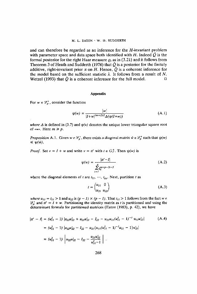
and can therefore be regarded as an inference for the H- invar ian t p rob lem with p a r a m e t e r space and data space both identified with H. I n d e e d Q is the formal pos ter ior for the right H a a r measure Or as in (3.21) and it follows f rom T h e o r e m 3 o f Hea th and Sudder th (1978) that Q is a pos ter ior for the finitely addit ive, r ight-invariant prior :r on H. Hence , Q is a cohe ren t inference for the mode l based on the sufficient statistic ~. It follows f rom a result o f N. Wetze l (1993) that Q is a coheren t inference for the full model . []

Appendix

For w E 9~ consider the function

Iwf ap(w) = (A. 1)

I I+wl (m+2) /2A(cp ( l+w ) )

w h e r e A is defined in (3.7) and cp(.) denotes the unique lower triangular Square root of ~~ Here m i> p.

P r o p o s i t i o n A. 1. Given w ~ ~ ; , there exists a diagonal matrix ~, ~ b~; such that ~p(w) -< ~0(g,).

P r o o f . Set v = I + w and write v = tt' with t e G~-. Then ~p(w) is

[ t t ' - l l ~p(w) - (A.2)

P .~ i i +P -2i+3 i=l

where the diagonal elements of t are tH, " ' , tpp. Next, partition t as

Ull 0 ) t = (A.3)

\U21 U22

w h e r e u t l = tu > 1 and u22 is (p - 1) • (p - 1) . That ttt > I follows from the fact w E 9~ and tt ' = I + w. Partitioning the identity matrix as t is partitioned and using the determinant formula for partitioned matrices (Eaton (1983), p. 42), we have

Itr - 11 = ( ~ , - 1)[u22u'22 + u2xu'2t - 122 - U2~UH(~ , -- 1 ) - ' U,U'2,1

= ( ~ t -- 1) lu22u'22 - 122 - u 2 ~ ( u , , ( u 2, - 1 ) - ' u H - 1}u~tl

(A.4)

I -- U21U~.___~ 1 ] = ( u f i - 1 ) !u22u' 2 - 122 "

268


However, the fact that tt' - I is positive definite implies that

U22Ul22 + U21Ul21 - - I22 - - U21UlI(U~I I - - 1 ) - l U l l U r 2 1 = U22Ut22 - - 122 - - _ _

is also positive definite so

U21U'21

u~l I - - 1

u22u'22 - 122

is positive definite. Hence,

Ill' - II <~ (u~t - 1) lu22u'22 - 1221 = (t~1 - 1) [u22u'22 - 1221. (A.5)

Now, repeat the above argument p - 1 times to conclude that P

Itt' - 11 <- 1-1 (t2ii - 1). (A.6) i=1

Finally, let r be diagonal with diagonal elements tffl - 1, -.-, ~p - 1. A bit of algebra shows that ~p(w) <~ lp(ff O. []

A c k n o w l e d g e m e n t

The au thors would like to thank the referees for a n u m b e r o f helpful com- ments which improved exposition.

R E F E R N C E S

BEaTI, P., REGAZZINI, E. and RIGO, P. (1991). Coherent statistical inference and Bayes theorem. Ann. Statist. 19, 366-381.

BERTI, P. and Rmo, P. (1994). Coherent inferences and improper priors. Ann. Statist. 22, 1177-1194.

Box, G. E. P. and TIAO, G. C. (1973). Bayesian Inference in Statistical Analysis. Addison-Wesley, Reading, MA.

EATON, i . (1982). A method for evaluating improper prior distributions. In Statistical Decision Theory and Related Topics III. S. S. Gupta and J. Berger (Eds.), Academic Press, New York.

EATON, M. (1983). Multivariate Statistics: A Vector Space Approach. Wiley, New York.

EATON, i . (1989). Group Invariance Applications in Statistics. Published by the Insti- tute of Mathematical Statistics and the American Statistical Association. [Confer- ence Board Publication sponsored by National Science Foundation].

269

M. L. EATON �9 W. D. SUDDERTH

FREEDMAN, D. and PURVES, R. (1969). Bayes method for bookies. Ann. Math. Statist. 40, 1177-1186.

GREENLEAF, F. P. (1973). Ergodic theorems and the construction of summing sequ- ences in amenable locally compact groups. Comm. Pure and Applied Math. XXVI, 29-46.

HEATH, D. and SUDDERTH, W. (1978). On finitely additive priors, coherence, and extended admissibility. Ann. Statist. 6, 333-345.

HEATH, D. and SUDDERTH, W. (1989). Coherent inference from improper priors and from finitely additive priors. Ann. Statist. 17, 907-919.

JAMES, W. and STEIN, C. (1960). Estimation with quadratic loss. Proc. Fourth Ber- keley Syrup. Math. Statist. Probab. 1,361-380, Univ. of California Press.

IZJEFER, J. (1957). Invariance, minimax sequential estimation, and continuous time processes. Ann. Math. Statist. 28, 573-601.

LANE, D. and SUDDERTH, W. (1983). Coherent and continuous inference. Ann. Stat- ist. 11, 114-120.

REGAZZINI, E. (1987). De Finetti's coherence and statistical inference. Ann. Statist. 15, 845-864.

STEIN, C. (1956). Some problems in multivariate analysis, Part. I. Technical Report No. 6, Department of Statistics, Stanford University.

STONE, M. (1976). Strong inconsistency from uniform priors. Jour. Amer. Statist. Ass'n 71, 114-119.

SODDERTH, W. (1994). Coherent inference and prediction in statistics. Logic, Metho- dology, and Philosophy of Science IX, editor D. Prawitz, B. Skyrms, and D. Wes- terst~hl, 833-844, Elsevier Science.

WETZEL, N. (1993). Coherence and statistical summaries. Ph.D. Dissertation, School of Statistics, University of Minnesota.

270

the formal posterior of a standard flat prior in manova is incoherent

Documents