The externalities from social housing

Evidence from housing prices

Antoine Goujard∗

(Job Market Paper)January 2011

Abstract

I investigate the impact of social housing on the sales price of neighboring flats in Paris. Iconstruct a unique dataset including flat sales and social housing projects at the building level.To account for endogenous placement of social housing projects, I use a difference-in-differencesstrategy that includes fine geographical controls and trending unobservables. In my preferredspecifications which control for building fixed effects, a particular spatial pattern emerges: a10 percentage points increase in the social housing share implies a 1.2% increase in housingvalue within a radius of 50 meters. However, private properties located farther away fromthe social projects within a 350 to 500 meter belt experience price decrease by 5.5%. Thepositive effects appear more important for small dwellings and for properties located in poorneighborhoods while negative impacts dominate in high income neighborhoods and for familydwellings. Further estimates exploit the unexpected win of a left-wing mayor in Paris, whichwas followed by a sharp increase in social housing units driven by the direct conversion ofprivate rental flats into social units without any accompanying rehabilitation. This naturalexperiment allows to identify the impact of the inflow into the neighborhood of low incometenants, separately from the effects of social housing on the quality of the existing housingstock. I do not find evidence of a positive impact of the conversion projects on housing prices.

Keywords: Social housing, neighborhood effects, housing prices.JEL Classification: J0, H42, R38

∗I thank my supervisors Barbara Petrongolo and Steve Pischke for guidance and support. I am gratefulto Julien Grenet, Radha Iyengar, Alan Manning, Guy Michaels and Henry Overman for helpful comments andsuggestions. The Commission of Parisian Notaries, the Centre Maurice-Halbwachs, the DREIF, the City of Paris,the APUR and the IAURIF provided the data. I thank Alain David who prepared the housing transactions data.All views and remaining errors are mine.Ph.D. candidate in Economics, London School of Economics and Political Science.Tel: +44 (0)20 7955 6907. E-mail: a.j.goujard@lse.ac.uk.

1

1 Introduction

Neighborhood effects and externalities are key issues in the social sciences and in the designof social policy. A large existing literature investigates the causes and impacts of neighborhoodand peer effects in a range of scenarios such as education, labor markets, health and crime1.Social housing is an important and growing component of social policy. Various countries haveseen an increasing Government involvement in this area at least partly motivated by the inten-tion to create or maintain mixed neighborhoods (see Currie, 2006, for the USA, Cheshire et al.,2008, for the UK and Laferrere and le Blanc, 2006, for France). However, there is little evidenceon the impacts of low-income housing developments on the neighborhoods in which they arebuilt.

While economists’ knowledge of the effects of social housing in local neighborhoods is stillrelatively thin (recent exceptions include Baum-Snow and Marion, 2009, and Schwartz et al.,2006), assessing such effects is crucial to compare the benefits of social housing for low-incometenants to the costs (if any) of creating and maintaining mixed neighborhoods. The overall ef-fect of social housing on nearby private housing is potentially ambiguous. On the one hand, bybringing in an inflow of relatively low-income residents, social housing affects the socio-economicmix of a neighborhood and may lower the value of the neighborhood to existing residents. Onthe other hand, project-based assistance that complements social housing projects may providean offset to the above effects, and more generally to urban decay. Rosen (1985) argues that so-cial housing units may be justified to replace distressed properties in low-income neighborhoodswhere social units may be better maintained than private rental units. Thus the effect of socialhousing concentration on local housing prices is ultimately an empirical question.

This paper estimates the impact of social housing on the private housing market, usinginformation on new housing developments and property sales at the building level for the cityof Paris between 1995 and 2005. I ask how proximity to social housing units affect the housingprices of nearby private flats and what are the underlying mechanisms. Paris provides a com-pelling setting to study the externalities of social housing for three main reasons. First, recentsocial housing policies in 2001 lead to a rapid expansion of the social dwelling stock with 18thousands social units, provided between 2000 and 2005. Social units accounted for 23.8% ofthe occupied rental housing stock at the end 1995 and nearly 27.3% at the end of 2005. Second,Paris is by far the most densely populated city in Europe, and as a result new social housingunits potentially affect a large number of private sales. I will be able to exploit the underlyingvariation using information on private sales at the building level. Finally, by comparing salesaffected by new constructions, rehabilitation of existing housing developments, or conversionof private housing, I can obtain a precise picture of the mechanisms driving the externalitiesstemming from social housing developments.

To analyze the effects of new social housing projects on neighboring private flats, I exploittwo complementary research designs. The first identification strategy builds on a difference-in-differences specification. An important contribution here is the introduction of a rich set of

1See among recent examples: Oreopoulos, 2003, Kling et al., 2007, Currie et al., 2010, Linden and Rockoff,2008, the review of Oreopoulos, 2008, and references therein.

2

local controls. Both developers and housing authorities have some control on the location ofnew social units and it is therefore important to control for unobserved determinants of projectlocation. In my difference-in-differences estimates, I can control for local unobservables downto the building level. Using the share of social housing within different neighborhoods as anexplanatory variable, I examine whether private flats located near social housing projects expe-rience different price changes once the social housing projects are created.

My difference-in-differences estimation strategy delivers two main results. First, withoutfine local controls the estimated impacts of social housing on housing prices is mainly negative.This mostly stems from the endogenous location of social housing in declining or deprived partsof small neighborhoods. When building fixed effects and local linear trends are included, theprivate housing stock located within 50 meters of the social housing projects experience positiveprice growth. Specifically, a new social housing project of typical size (35 units) raises localhousing prices by around 2.6% and a 10 percentage points increase of the social housing shareraises housing prices by about 1.2%. The timing of these effects is consistent with a causal im-pact and the estimates are robust to the inclusion of local linear trends. This result challengesthe belief that the potential inflows of low-income tenants could offset the benefits of the reha-bilitations and new constructions associated with social housing projects. Second, the impactsof social housing projects appear either close to zero or negative for private flats located fartheraway from the projects. For neighborhoods located 350 to 500 meters away from the socialprojects, a 10 percentage points increase in the social housing share (corresponding to aboutone standard-deviation change) would imply a 5.5% decrease in housing values. These averageeffects are the result of important heterogeneity with respect to neighborhood’s characteristicsand dwelling size. The positive impacts measured within 50 meter of the projects are drivenby small flats in low-income neighborhoods, while the negative externalities measured withinthe outer belt from 350 to 500 meters are mainly driven by family dwellings and high incomeneighborhoods.

To investigate the mechanisms driving these externalities, I exploit the election of the cur-rent mayor, Bertrand Delanoe, in March 2001. The Delanoe administration marked a sharpincrease in the number of social units and a change in their usual channel of provision fromnew constructions and rehabilitations of distressed private properties towards the conversion ofprivate rental properties into social units. As these direct conversions (acquisition sans travaux )do not involve new buildings or rehabilitations, they allow me to identify the effect of the inflowinto the neighborhood of low income tenants, separately from the effect of social housing onthe quality of the existing housing stock. This policy experiment points towards zero effects oflow-income tenants inflows.

This paper builds on the research assessing externalities of housing policies in the privatehousing market. A first stream of this literature is based on difference-in-differences estimationstrategies controlling for census tract or block unobservables. Schwartz et al. (2006) investi-gate the effects of subsidized housing projects in New York between 1987 and 2000. Usinga difference-in-differences hedonic regression at the census tract level, they define the houseslocated within 600 meters of a project as treated. They find that both rental and owner oc-cupied subsidized housing projects tend to have large positive externalities, mainly due to the

3

construction of new buildings and the removals of disamenities in distressed neighborhoods.Santiago et al. (2001) find similar results for the dispersed housing subsidy program in Denverwhich led to an increase in small scale rental projects over the period 1987 to 1997. Autor et al.(2009) analyze the effects of the elimination of rent control in Cambridge (USA) during 1995-1997 and document negative externalities of rent controlled properties on neighboring houses,having controlled for detailed property characteristics. Hartley (2008) finds that the timing ofclosures and demolitions of high rise public housing buildings in Chicago is associated with anincrease in housing prices in the vicinity of the past projects, consistent with the removal ofdisamenities.

Baum-Snow and Marion (2009) tackle more directly the issue of the endogenous location ofthe new social housing projects. They exploit a discontinuity in the formula for the eligibilityfor Low Income Housing Tax Credit (LIHTC) subsidies, which creates quasi random variationsin the number of new buildings between census tracts. Their regression discontinuity designshows that additional new projects and LIHTC tenants stimulate home-ownership turn-over,housing prices in declining areas and lower median income in poor gentrifying areas.

My identification strategy differs from both the usual difference-in-differences strategies andBaum-Snow and Marion (2009) in three important dimensions that are likely to explain the dif-ference in my findings. First, most papers have used aggregate census data at the tract level2,while my data gives me the exact location of each sale and each new social housing unit. Thisspatial richness allows me to get a more detailed picture of spatial spillovers and to control forbuilding unobservables. This is important when the effects considered are extremely localizedand if the location of new projects is endogenous within census tracts. Second, the regressiondiscontinuity design adopted by Baum-Snow and Marion (2009) focuses their analysis on theimpacts of social housing in poor neighborhoods, while Paris is one the wealthiest city in Eu-rope, the median pre-tax household income ranging from 13, 985 euros in the poorest censustract to 61, 783 euros in the highest in 2001. This allows me to uncover heterogeneous effects ofsocial housing on housing prices. Third, most of the point estimates provided by the existing lit-erature reflect the combined impact of the revitalization effects of new housing projects and theinflows of low-income tenants into a neighborhood. The Parisian set-up allows me to distinguishbetween the impact of new social housing created via new constructions and rehabilitations ofexisting dwellings and that of straight conversions of private rental units into social housing andtherefore more closely isolate the impact of additional poor households on neighborhoods.

The paper is organized as follows. The next section discusses the features of Parisian socialhousing that are relevant for my analysis, describes data construction and some summary statis-tics. Section 3 describes my identification strategies. Section 4 describes my main empiricalfindings on the externalities of social housing on private housing prices. Section 5 investigatesfurther the mechanisms driving these externalities. Section 6 concludes.

2For example, Baum-Snow and Marion (2009) use US census data at the tract level and define neighborhoodas a 1-km circle around the census tract’s center. Chay and Greenstone (2005) and Greenstone and Gallagher(2008) use comparable data.

4

2 Institutional background and summary statistics

2.1 Institutional background

The Parisian social housing system is based on rental units subsidized by low interests loansand tax deductions. Housing units are owned by private local companies, HLM 3. Despite theirprivate status, these companies are closely monitored by the central government and the mu-nicipality, that sometimes contribute to rehabilitation, maintenance or demolition of buildings.Moreover, in Paris, the municipality is the main joint owner of the largest HLM companies.

Project-based assistance is used by HLM companies to create new social units either throughsubsidized construction, rehabilitation or conversion of private buildings4. Once a social housingunit is created, it remains in the social sector forever5. Figure 1 breaks down the number of newunits created in Paris from 1970 by year of completion and type of creation. The timing andtypes of the new units match closely the city mayoral elections that took place every six yearsfrom 1977 to 2001 and in 2008. The overall production of social dwellings is lower after thechange of mayor in 1995 and increases significantly after the first election of a left-wing mayorin 2001. Until 2001, the main method to create new social housing units was new buildings.During the 1980s the rehabilitations of existing distressed properties increased significantly. Atthe same time, figure 1 reveals a sharp decline in the number of social units created through newbuildings during the 1990s, from an average of approximately 2, 700 annual new dwellings atthe end of the 1980s, to an average of 900 new dwellings between 2000 and 2010. The purchaseof 20 year old buildings without any rehabilitation was only authorized by a change in law in20016. From 2001, rehabilitation of existing properties and conversions of private rental flatswere the main methods used to increase the stock of social dwellings.

The French Government has designed several incentives for each municipality to develop acomparable stock of social dwellings. A law adopted in 2000 imposes a minimum share of 20%of social housing units among the occupied housing stock in each municipality and thereforeParis, with a social housing share of 13.1% in 2001, is directly concerned7. However, the spatialdistribution of social housing inside Paris is a joint decision of the HLM developers and themunicipality. The municipality intervenes through the selling of public land and buildings todevelopers, the authorization of new buildings and the design of the subsidies that add non-trivial monetary and non-monetary incentives to the location of new social units. The mainobjective since 2001 has been to reach a better spatial distribution of the social housing stock.The municipality decided to apply the 20% limit to all the arrondissements in Paris and createdan inclusionary zoning which stipulates that any large private project located in central Parisshould incorporate at least 25% of social dwellings. Figure 2 plots the location of the new units

3Habitations a loyer modere.4HLM companies were allowed to buy a minority of dwellings of private new projects before their completions

(VEFA) by the decret 2001-104 (08/02/2000).5The French government created incentives for HLM companies to sell social units to their low-income tenants.

The main HLM companies in Paris do not apply this policy.6Decret 2001-336 (18/04/2001) for the financing of PLUS dwellings and Prefecture de Paris (2004). The

purchase of existing buildings for PLA-I was authorized earlier by the Decret 1990-151 (16/02/1990).7Recently, Glaeser and Gottlieb (2008) advocate the use of subsidized housing in the USA to increase the

supply of affordable housing in highly productive areas.

5

over time. Small dots represent social housing projects created before 2001 and larger dots theprojects created after 2001. The conversion projects created after 2001 are represented by largesquares. The underlying map presents the median housing price (per square meter) in 1995.Overall a negative correlation appears between the number of projects and housing prices. In-terestingly, recent projects are spread throughout the city while older social housing units arelocated in fewer neighborhoods. The unequal distribution of the variation in the social housingshare across the city would pose problems in the presence of localized shocks (e.g. renewal pro-grams, industrial clean-ups etc.). The widespread distribution of the new social housing unitsmitigate the influence of these local shocks.

The expected impacts of social units on surrounding properties depend crucially on thecharacteristics of the social dwellings. Each dwelling is subject to some level of rent controlaccording to the subsidies used to finance the project. HLM companies have a restricted choiceover the eligible tenants who are determined mainly through income, number of children andprevious housing (Laferrere and le Blanc, 2006). As a priority is given to households in finan-cial difficulties, the income of the successful applicants appears far below the maximum incomelevels. Allocation of the two main types of social housing published by the municipality in 2005shows that the income of the new tenants was below 60% of the usual income threshold in 90%of the cases (APUR, 2006). Hence, new social tenants are typically below the 20th percentile ofincome by consumption unit8.

Table 1 summarizes the characteristics of the HLM dwellings and tenants with respect tothe private accommodation sector according to the French Housing Survey in 2002. The firstcolumn shows the characteristics of the stock of social housing dwellings, the second showsthe characteristics of the social dwellings with new tenants9 while the last two columns showthe characteristics of private rental dwellings and owner occupied dwellings. Panel A providesinformation about the structural characteristics of the units. Social dwellings are located inlarger and more recent buildings: 19% were built after 1982 against 7% in the private rentalsector or 4% for owner occupied units. They are also larger than private rental units by around25% or 0.6 rooms and located in larger buildings. The average rent by square meters in thesocial sector is less than half the rent in the private sector. As a result of this rent differenceand the scarcity of the social offer, the duration of tenancy in the social sector is greater thanin the private sector by 5 years.

Panel B of table 1 displays the main characteristics of the social tenants. The income byconsumption unit of the social tenants is one third, approximately one standard-deviation, be-low the corresponding average in the private rental sector. This lower level of income is relatedto larger shares of non qualified, unemployed and inactive individuals. Social tenants are alsoolder and less likely to be born in France than households in private accommodation. Theshares of families and single parents are also significantly higher.

Finally, panel C of table 1 reports the opinion of the households on the neighborhood andmaintenance of social dwellings. Flooding appears less of a concern in the social sector asthe buildings are more recent. However, 38% social tenants report that the building has been

8Eurostat consumption unit. There are large variation of eligibility level by household size.9I define as new tenants the households who moved in during the last four years.

6

degraded last year while this number is only of 18% in the private sector. The number ofhouseholds that declares being victims of robberies (or attempts) is also substantially higherthan in the private sector. While the average social tenant thinks that his neighborhood is lesssafe than the average private tenant, new social housing tenants have a more positive view ofthe neighborhoods of their social units.

Due to the difference in households’ income and the characteristics of the social buildings,investments in low-income housing could have different externalities according to both construc-tion types, level of income of the tenants and initial neighborhoods. Depending on the projects,the main spillover effects could be through the low-income tenants living in social housing, theupgrade of existing buildings or through complementary investments. For example, social hous-ing units are often created through urban renewal operations and associated with new publicfacilities such as new roads, additional playgrounds or schools’ investments.

2.2 Data and summary statistics

The definition of social housing adopted in this article is restrictive, it closely follows theFrench law of 2000 (SRU ). Social units belong to an HLM landlord and receive an agreementfrom the state which give rights to construction and rent subsidies in exchange for some levelof control on the rents and the choices of the tenants10. The only exception are the dwellingswhich belong to the HLM companies since 1977 or before. As formal rental agreement (conven-tionement) did not exist before 1977, all these HLM rental dwellings are considered as socialhousing. Furthermore I restrict the sample of projects to the family dwellings excluding the fewstudents’ residences, collective accommodation for the elderly and temporary accommodationfor the homeless11. These restrictions are motivated by the fact that these social housing unitsrepresent a very small fraction of the inflows and are not considered as social housing in theavailable surveys or in the existing literature.

The public housing stock and its evolution is constructed from seven yearly exhaustive sur-veys completed by the regional planning agency (DREIF ). These surveys are mandatory andwere carried out in 1998, 2002, 2003, 2004, 2005, 2006 and 2007. Each year the planning agencyasks the HLM landlords to update a description of their social housing dwellings. The resultsare used to compute tax transfers to municipalities and as planning instruments for the publichousing policy at national and local levels. I have complemented these surveys by administra-tive records from the City of Paris which contain the same information on a more recent period.This dataset tracks the new and planed social housing units from 2001 to 2012 as of June 2007.In the two data-sets, projects are defined by an address, a subsidy type and a year of comple-

10There is no unique definition of the social housing stock. The French census, housing surveys and adminis-trative records use different definitions (see data appendix, CNIS, 2001 and Briant et al., 2010).

11In the French 2000 law, these types of housing are considered as social housing. Each bed or room has aweight that is a fraction of a family dwelling.

7

tion12. Information on each project include: the completion year13, the year of agreement, theaddress and the number of dwellings by level of subsidy. The completion and agreement of theprojects are only known up to the year level. The completion year corresponds to the year of thefirst occupancy of the building by a social tenant. The agreement year is the signing year of theformal subsidy agreement between the State and the HLM company (conventionnement). Theamount of time between these two dates depends crucially on the mode of provision of socialhousing units, from less than a year for the conversion of existing private rental properties intosocial units up to an average of three years for new buildings or rehabilitations. The createddataset is then matched to the geographical location using the addresses of the buildings toleave me with an address-year panel of the social housing stock.

Data on property sales are from the Commission of Parisian Notaries, BIEN dataset14. Thedata has been used to produce official statistics, evaluate the impact of school quality (Fack andGrenet, 2010) and the efficiency of urban renewal projects (Barthelemy et al., 2007). In France,each property sale has to be registered by a Notary who is in charge of setting up the contractand collecting taxes for the State. The sample is restricted to arm’s-length sales of Parisianflats without occupant owner. The transactions data set is almost comprehensive from 1995 to2005 and contains 333, 590 flats transactions inside Paris. The INSEE evaluated the coveragerate of all housing transactions in Paris at 90% in 2004 (Gourieroux and Laferrere, 2006)15. Asmy outcome variable is the log price, the quality of the information on prices is a main issue.The reported prices may be biased by tax evasion and money laundering. The French NationalAssembly notes that the permissive regulation of French property-owning companies is the mainsource of fraudulent transactions in the real estate market (Assemblee Nationale, 2002). Thisissue is less tangible for the sales between private households. In 95% of these sales, a falseprice record would require collusion between four parties: the buyer, the seller, the real estateagent and the notary (OECD, 2008). As a result, I restrict my sample to the sales between pri-vate households. The sales between private households represent 231, 803 transactions (69.5%of the initial sample). This restricted sample avoids the problem of sales to and from HLMcompanies and other administrative bodies. However these restrictions discard the sales fromdevelopers to private households occurring in new buildings that may be located close to socialhousing projects in urban renewal programs. In the empirical section, I present evidence thatthese restrictions do not imply sample selection issues. The sales located close to social housingprojects are not more likely to have private buyers before or after the projects’ completion.Furthermore, the number of sales at the building level does not depend on the local evolutionof the social housing share.

12The same address or building may contain units financed by different subsidies. This represents severalprojects in my data.

13I corrected two obvious mistakes. First, there were two main mergers between HLM companies and someof the buildings were recorded at the merger year in the following surveys. Second, early HLM, HBM buildings,were described as completed at the time of a public renovation. I recoded them at the time of construction. Someof the projects started in 2007 were not completed. I used the estimated completion year provided by the Cityof Paris in 2007.

14Base d’Informations Economiques Notariales.15This number is for the whole universe of housing transactions and does not distinguish private households

from firms or public bodies.

8

The control variables include the characteristics of the flats and the sales, namely: size,number of bedrooms and bathrooms, date of construction of the building, day of the sale andthe address. Each address was located in Lambert grid coordinates (Lambert 1 North) bymatching on its exact name16. Table 2 provides broad descriptive features of the flats sold inParis in 1995 and 2005: for the whole sample, for the flats sold between private householdsand repeated sales within the same building. Panel A shows the characteristics of the flats.There was first no independent check on the accuracy of the dwellings attributes17. This isparticularly striking for the dwellings’ size, as nearly half the information was missing in 1995.As data quality control increases, there was less than 10% missing values for the same attributein 2005. During the sample period the average price per square meter in 2005 euros increasesby 100% between 1995 and 2005, while the number of sales also increases twofold from 1995 to2000 and remains stable afterwards. The main characteristics of the sales remain homogeneousover the sample period. The average flat is around 51 square meters, 60% of the sold propertieshave one or two rooms and 90% of them were built before 1992. Interestingly, 90.1% of thesales between private households (208, 918) occur within buildings18 having at least two sales(between private households). Consequently, it is reassuring that my results based on controlsat the building level will not be driven by a small subsample.

Panel B of table 2 presents the main explanatory variable of my analysis. It was constructedby combining the precise geographic coordinates of sales and the mapping of new social housingprojects. To describe the relative intensity of social housing in the vicinity of a sale i at time t,I define different neighborhoods by distance d. Sit(d) represents the share of social housing inthe neighborhood of sale i with respect to the number of flats in the same circle according tothe last comprehensive census in 1999:

Sit(d) =Hit(d)Ni(d)

, (1)

where Hit(d) is the number of social housing units completed at or before time t within a circleof radius d around the flat and Ni(d) is the estimated number of occupied flats in the circle ofradius d according to the census in 1999. The break-down of the number of flats at the tractlevel is the smallest publicly available data from the 1999 census. Thus it is not possible to geta direct estimate of Ni(d). Figure 3 illustrates the process used to compute the social housingshare. It shows a map of the 13th arrondissement in Paris. Plain lines represent census blocksand dots the social housing buildings in 2010. Three circles of 50, 250 and 500 meter radii arecentered around a particular sale. For each circle, Ni(d) is the sum of the occupied dwellings

16Incorrect spellings were manually corrected. The main remaining mistakes were corrected using local tax lots(parcelles cadastrales) and additional location information (complements d’adresses). The spatial location has aprecision of the order of five meters. The addresses were matched to the census blocks (Ilots) and tracts (IRIS)that are clusters of blocks using the French statistical office coding file. In Paris, census tracts represent smallareas of around 2, 500 inhabitants and census blocks have an average of less than 500 inhabitants.

17The French statistical office now produces quarterly housing prices using these data.18I define a building as the intersection of an address and a period of construction. According to this definition,

69.6% of the addresses have a unique building (89.5% for the repeated sales sub-sample). Using building ratherthan address as the unit of analysis has the advantage of not considering demolition and new construction onthe same address as an upgrade of an existing entity. In practice, the results are not sensitive to using buildingor address fixed effects once I control for the period of construction of the buildings.

9

over all intersected census tracts, each tract being weighted by the fraction of its area locatedwithin the circle19.

In Panel B of table 2, the average transacted flat in 1995 has 10% of social housing unitswithin 500 meters. This number decreases slightly once smaller circles of 350, 250, 150 and50 meter radii are considered. Within the smallest geography of 50 meters, the social housingshare in 1995 is 7%. This pattern is very similar in the cross-sections in 1995 and 2005. Itcorresponds to the spatial bunching of social housing units in a few neighborhoods observedin figure 2. The circles are centered around private properties and the smallest radius of 50meters takes only into account immediate neighbors which are less likely to be social housingunits. Furthermore, the standard-deviations of the radial measures of the social housing shareare increasing when I consider smaller radii. In 1995, the standard-deviation of the 500 metermeasure (0.10) is nearly five times lower than the standard-deviation for the 50 meter measure(0.46). However, all the radial measures display a similar evolution from 1995 to 2005. Overthe sample period 1995 to 2005, the share of social housing in the housing stock increases by27, 773 units or 2.5% of the occupied housing stock in 1999.

The last row of table 2 gives the evolution of an alternative measure of the social housingshare. This measure uses a parametric definition of neighborhood: the census tract of the 1999census. I consider the total number of social units located in each tract. The denominator ofthe census tract measure, Ni, is known without uncertainty. The descriptive statistics for thismeasure are close to those obtained for a circle of radius 150 meters. The median size of a censustract is indeed equivalent to a circle of radius 146 meters. However, from figure 3, the radialmeasures of the social housing share have two main advantages. First, they can be computedat different geographical levels. Second, the census tract boundaries follow the middle of thestreets. Thus the crossing of a street implies a partly artificial discontinuity in the measuredsocial housing share.

3 Empirical strategy

3.1 Main specifications

Exposure to social housing varies across time and location. This paper seeks to identifya traditional hedonic equation where the log-price of a flat sale is related to the flat’s variouscharacteristics:

ln(pibgt) = xibgtβ + γSbt(d) + αgt + εibgt , (2)

where i is an index for flats, b for buildings, g for various geography levels and t for time. xibgt isa row vector of observable dwelling characteristics that may affect housing prices. Specifically,xibgt includes number of rooms; size in square meters; floor; age of the building; and dummyvariables if the flat has a bathroom, a parking lot, a cellar or a lift. Sbt(d) is the share ofsocial housing dwellings in the neighborhood of the building within a given radius d and αgt

19The implicit assumption that the density is constant within census tract is likely to approximately hold inParis. The regulation of building height, epannelage, is strictly applied.

10

represents geographical unobservable characteristics. My main specifications correspond to adifference-in-differences set-up where αgt = δg + αt.

OLS estimates of the impact of public housing on housing prices are unlikely to identify γ,the parameter of interest, because Sbt(d) may be correlated to unobserved neighborhood char-acteristics or unobserved characteristics of the dwelling through αgt or εibgt. This identificationproblem is difficult to circumvent for three main reasons.

First, the location of social housing projects is a joint decision between the HLM developersand the municipality. As the rent of social units is fixed at the city level, landlords have incen-tives to target distressed properties and neighborhoods with low or declining housing values20.Similarly, the municipality may value the removal of slums and their replacement by publichousing. Thus, the specific unobservables of the private properties surrounding social housingprojects may differ from the characteristics of properties not affected by the projects.

Second, the timing of the effects of new social housing dwellings is ambiguous. Changes inneighborhood composition could be anticipated by buyers and sellers. Social housing buildingstake an average of three to four years to be completed after the initial agreement and, in thecase of new buildings, public hearings are mandatory. Furthermore, there is a time lag betweenthe flat buying decisions and the recorded time of the sales.

Third, the local public housing stock may evolve jointly with other factors having directimpacts on dwellings’ values. For example, new public housing projects may be accompanied bybetter transportation links, infrastructure investments and new commercial or public services.These complementary investments could be planed by the municipality or the result of a politi-cal process. Anecdotal evidence suggests that the affected populations may organize themselvesto lobby local governments and HLM companies in order to obtain various forms of compen-sation or amendments to the initial projects (Paris, 2006). Developers may also target newsocial buildings according to adverse neighborhood shocks such as fire or lack of maintenance ofnearby buildings. Mean reversion could also bias upwards the measure of the impacts of socialhousing on nearby private properties. Even in the same census tract, the characteristics of thesales before and after the creation of social housing units may differ in a systematic mannerwhich would bias difference-in-differences estimates. Finally, the observed changes in price maybe driven by changes in the own characteristics of the dwellings such as buildings’ upgrades, orby changes in the valuation of observable dwelling’s characteristics.

To circumvent the endogeneity of location problem, I take advantage of the high populationdensity in Paris to control for local unobservables. Most previous papers have considered thegeographical unit of interest g as a census aggregate (tracts, blocks or counties)21. I extendthese geographical controls by defining my smallest geographical unit at the building level. Pre-cisely, I define a building as the interaction between an address and a period of construction.This allows me to control for numerous time invariant characteristics of the dwellings. Forexample, Parisian school catchment boundaries do not follow census tract definition (Fack and

20Anecdotal evidence suggests that most HLM companies do not take into account the potential residualmarket value of social properties when they compute the expected returns of social housing projects (InspectionGenerale des Finances and Conseil General des Ponts et Chaussees, 2002).

21In most set-ups, repeated sale specifications imply some issues of sample selection.

11

Grenet, 2010) and most of the major investments that could impact sales prices take place at thebuilding level (e.g. water provision, sanitation, lift maintenance etc.). Moreover, building fixedeffects mitigate a main source of time varying unobservables that may be correlated with thesocial housing share. The replacement of distressed private buildings by new private buildingsis not confounded as a neighborhood upgrade.

A first test of the causality of the estimates is to generalize regression (2) by allowing theexternalities of social housing to decay with the distance to the projects. In this case, the effectsof the social housing projects are measured by a vector (γr) corresponding to the impact of thesocial housing share in different rings (r) around a sale:

ln(pibgt) = xibgtβ +∑

r

γrSbt(r) + αgt + εibgt (3)

where the ring variables Sbt(r) are mutually exclusive and define concentric belts with differenttreatment intensities. I would expect to see larger effects for private properties located closer tothe social projects because they have a more direct exposure to the potential buildings’ upgradesand inflows of low income tenants.

I address the problem of the timing of the impacts by allowing the effects of interest todepend on the completion date of the projects. As the same transaction can be affected byseveral housing projects occurring at different points in time, I need to consider the inflows ofsocial housing units over time and not pre and post treatment dummy variables. Specifically, Iintroduce lead and lag flows of social housing divided by the number of flats in the neighborhoodin 1999. Fb,t+2c(d) represents the additional share of social housing due to projects completedbetween 2(c− 1) and 2c after the time of the sale, t, within a circle of radius d. I use two yearchanges to ensure sufficient variation even within small neighborhoods. These new variablescan be expressed in terms of the share of social housing within a circle of d meter radius at timet, Sb,t(d):

Fb,t+2c(d) = Sb,t+2c(d)− Sb,t+2(c−1)(d) . (4)

For example, Fb,t−2(d) takes into account all projects completed two and three years prior tothe sale at time t and Fb,t(d) measures the inflows of social housing units during years t andt− 1. The final regression corresponds to:

ln(pibgt) = xibgtβ + γiSb,t−14(d) +3∑

c=−6

γcFb,t+2c(d) + αgt + εibgt . (5)

This specification assumes that projects built more than 14 years before the time of the saleshave a constant impact on housing prices (γi) and that projects that will be built more than6 years after the sale can not be anticipated by the housing market. Under the assumptionthat flats and neighborhoods unobservable characteristics do not evolve systematically with so-cial housing inflows, the γc’s measure the differential impact of the closeness to social housingdwellings with respect to the year of completion of the projects. Specification (5) can be ex-tended as specification (3) to incorporate heterogenous impacts on housing values by distancebelts.

12

I test the robustness to potential time varying unobservables correlated with the social hous-ing share by including local linear trends at different geographical levels. In my most flexiblespecification, this heterogenous growth model includes controls for building unobservables andcensus tract linear trends.

To get an idea of the precision of my local controls, it is useful to compare the geographyof Paris to the one used by Schwartz et al. (2006) to evaluate the externalities of subsidizedhousing in New-York. The smallest level of the French census is the block for which no publicdata are available. French census tracts are small clusters of blocks that are designed for therelease of statistical information. The French census tracts match the main political units. Eachof the twenty arrondissements of Paris are divided into four administrative quartiers which aresubdivided into census tracts. A direct comparison of the 2000 US census and the 1999 Frenchcensus show that the typical Parisian tract is much smaller than the average New-York tract:the population is on average one third below and the area five times smaller. In terms of area,the average Parisian census tract is also between the Chicago census block groups and censusblocks considered by Autor et al. (2009).

3.2 Isolating the effects of low-income tenants

The previous specifications have two remaining shortcomings. First, they estimate an ag-gregate impact: the creation of new social units through rehabilitation and new buildings andthe inflow of low income tenants. Second, even after controlling for local trends, disentanglingsocial housing effects from local complementary investments is not straightforward. In orderto obtain a more precise idea of the effects of low income tenants on housing prices, I exploitvariation in the stock of social housing units following the election of the current mayor in 2001.The current mayor of Paris, Bertrand Delanoe, was virtually unknown before his electoral winin 2001. This electoral poll was close and uncertain: at the second round of the election, theleft-wing alliance received 49.6% of the votes against 50.4% for the divided right wing.

Following this electoral win, a sharp increase in the provision of social housing units wasachieved through the conversion of existing buildings into social housing units (Figures 1 and2) or acquisition sans travaux 22. There were no conversion projects before 2001. These projectswere not accompanied by new construction or rehabilitation and thus one can infer that theireffects on housing prices were limited to the inflow of low income tenants into the neighbor-hoods and the consequent changes in their socio-economic compositions. Bacquet et al. (2010)describe the new process for two projects in Paris based on interviews with the tenants. TheHLM company or the municipality buys an existing rental building from private landlords usingsocial housing subsidies. The vacant flats are allocated to HLM applicants and the remainingprivate tenants are slowly replaced by HLM households when they leave the building or theirtenancy expires. This process was particularly controversial as it was judged costly in respectto the other ways to provide social housing. Moreover, it was mainly used in wealthy neigh-

22This process is also known as acquisition conventionnement.

13

borhoods to create dwellings for very low income households. The APUR (2010)23 providesdescriptive statistics from a survey of the HLM landlords of converted buildings in April 2009.During the first two years after the mayoral election, 3, 933 social dwellings, more than 60% ofthe total number of agreed dwellings, were created using this financing scheme. At the time ofthe survey, 80% of these dwellings were occupied by social tenants. From 2001 to 2005, 6, 913private dwellings were converted into social housing units.

I use this policy shock to isolate the impact of the share of social tenants in the neighborhoodof the sales. This policy has two main advantages. It was arguably unpredictable by home-buyers of nearby sales and it is not systematically associated with other public investments inthe neighborhood of the sales. From the data provided by the City of Paris, I construct theevolution of the share of the converted social housing in the occupied housing stock in 1999from 2001 to 2005 as in equation (1).

4 Empirical results

4.1 Cross-sectional estimates and parametric neighborhood definition

Table 3 shows how the log price of sales (in 2005 euros) changes with existing and futuresocial housing projects from 1995 to 2005. The sample is restricted to the sales occurring withinbuilding with repeated sales to ease the comparison with the estimates controlling for buildingunobservables. I use my two alternative measures of the social housing shares: by radii from500 meters to 50 meters in columns (1) to (4) and within census tract in column (5)24.

The regressions in panel A control only for the time of the sales. These cross-sectional esti-mates reveal that housing values are negatively correlated with the share of social housing in thevicinity of the sales. This conclusion is robust to the neighborhoods I consider. The magnitudeof the cross-sectional estimate at 500 meters indicates that an increase in the share of socialhousing by 10 percentage points (approximately one standard-deviation) is correlated with adecrease of 14% in housing prices. The negative impact of social housing on housing prices isdecreasing with the closeness to the sales even if the standard-errors remain low. When thesocial housing share is measured only within 50 meters to the sales, the cross-sectional pointestimate is divided by 21. However a one standard-deviation increase of the share of socialhousing within 50 meters would still imply a significant decrease in housing price by 2.6%. Asimple computation can help to get a better sense of the size of the measured effect. As the av-erage property has 161 surrounding flats within 50 meters, an average project of 35 flats woulddecrease the property value by 1.4%. The census tract measure of the social housing sharedoes not provide a different picture from the radial measures. As expected from the descriptivestatistics, the point estimates and standard-errors match closely the results obtained for the150 meter radius.

23Atelier Parisien d’URbanisme.24As the pattern of the point estimates is smooth over radii, table 3 does not report the estimates for the 350

meter measure to save some space. Table A1 presents descriptive statistics for the social housing share measuresby circles and belts around the sales.

14

The second and third rows of panel A investigate further the causality of these point es-timates. In row 2, the negative point estimates are stronger when the social housing includesonly the projects created within the past 10 years. The point estimate for the 500 meter radiusis multiplied by 7 and the one for the 50 meter radius by nearly 2. New social housing projectsappear to have more negative externalities than existing low income housing. This could beconsistent with more negative externalities. New social tenants are poorer than establishedtenants and new social housing dwellings have more stringent income eligibility requirementsthan HLM created before 1977 (table 1). However, no causal interpretation can be given to thisphenomenon. New social housing projects may also be located close to private housing havingworse observable and unobservable characteristics than older projects. In row 3, housing pricesare also correlated with future social housing units which will be built in the next five years.Interestingly, the magnitude of the point estimates in columns (2) and (3) are close. Withinthe 50 meter radius, the effect of the future social units is more than twice as high as that ofthe current units. Flats located in neighborhoods where the share of social units will increaseby 10 percentage points in the next five years have 2.6% lower values. On the one hand, thetime pattern of the point estimates could be consistent with the fact that social dwellings arelocated in large deprived neighborhoods and tend to replace distressed properties at the locallevel. On the other hand, the same pattern could also be consistent with rational expectationsof the home buyers if they are able to predict future social housing developments.

In panel B, I introduce an extensive set of controls for flats characteristics25. The esti-mated coefficients decrease slightly in absolute value but are also more precisely estimated. Thesmallest estimate at 50 meters still implies that a new social housing project would decreasehousing values by 1.1% and it remains significant at the 1% significance level. In summary, thelinear covariate adjustment leads to similar results as the specification without these controls.Although the set of controls is large, it may not be adequate to solve the endogeneity of thenew projects’ location. To isolate the causal impact of social housing on housing prices moreprecise local controls may be needed.

4.2 Geography fixed effects

Table 4 presents the results of the difference-in-differences specifications (2) to (4) at vari-ous geographical levels: 80 quartiers, 902 census tracts and 36, 274 buildings26. The idea is tocontrol for the particular local characteristics around social housing projects. All regressionsinclude an extensive set of controls for the flat characteristics and the time of the sales. I usemy main measure of the social housing share: by radii from 500 meters to 50 meters. Columns(1) to (3) introduce the share of social housing within 500 meters of the sales, columns (4) to(6) within 250 meters, columns (7) to (9) within 150 meters and columns (10) to (12) within50 meters.

Panel A of table 4 does not control for different house price trends around the social housing25Table A2 presents the specification and the summary statistics for all the control variables included.26For all specifications, the sample is restricted to the sales between private households occurring within

buildings with repeated sales. Controlling for building fixed effects or address fixed effects does not affectsignificantly the point estimates.

15

projects. While using quartier or census tract controls, the estimates appear consistently nega-tive, their sign changes once the fixed unobserved characteristics of the buildings are controlledfor. Column (1), the point estimate using quartier fixed effects indicates that an increase of10 percentage points of the share of social housing within 500 meters would decrease housingvalue by 6.0%. This estimate is divided by two, a 2.8% decrease, when I control for census tractfixed effects in column (2). However, once I control for building unobservables, column (3), Iobserve a different story in Paris. The same change would imply a 3% increase in housing value.The price increase estimate is statistically significant at the 10% level. At the same time, theR-squared rise from 0.871 to 0.911 when building rather than census tract controls are included.This means that building and precise location characteristics play a key role to determine bothhousing prices and social projects’ location. The change in the values of the point estimates andR-squared across fixed effects from quartier to building is consistent over the different radii.

Focusing on the specification controlling for building unobservables and variation within the50 meter circle, column (12), the positive impact of the share of social housing within 50 metersof the sale is statistically significant at the 1% level. A new social project of 35 flats wouldimply an increase in housing value by 1.4%. As projects are associated with new buildingsand rehabilitations, positive estimates could correspond to disamenity removals and buildings’upgrades at a small spatial scale. Based on census tract controls, the estimates for the impactof the share of social housing on housing price seem to be biased by omitted variables andhave a negative sign. The social housing share is proxying for buildings having worse unobserv-able characteristics. However, the positive estimates are consistent with another story relatedto time varying unobservables. The creation of social housing units could be associated withcomplementary investments in small neighborhoods, such that additional playgrounds or newpublic services. Even controlling for building fixed effects, the estimates of the impact of thesocial housing share could be confounded by mean reversion and the selection of locations withparticular underlying price trends.

Panel B of table 4 presents the results of the same specifications as panel A but including 80quartier linear trends27. In all the fixed effect specifications the overall impact of social housingappears similar to the estimates reported in panel A. At the same time, the R-squared for allthe regressions are not affected by the inclusion of these trends. The quartier trends explainneither the location of social housing nor the evolution of the log housing price.

Table 5 presents the results of the difference-in-differences specification (3) that investigatesfurther the causality of the relationships of table 4 by introducing the share of social housingwithin different belts around the flats. As the share of social housing in the different belts aremutually exclusive, each coefficient represents the effect of the social housing share in a givenbelt. Estimates in columns (1) to (3) condition on flat controls, time of the sales and geographicfixed-effects, while the specifications in columns (4) to (6) also include 80 quartier linear trends.In columns (1) and (2), with geographical controls at the quartier or tract levels, the spatialpattern of the point estimates is not consistent with a negative externality centered around theprojects. The estimate for the 350 to 500 meter social housing share in column (1) is nearly 20times higher than the point estimate for the 50 meter circle. The pattern of the standard-errors

27The linear trends are measured as the number of days between the sale and the 31st December 1994.

16

is also informative. Given that the 350 to 500 meter ring is much larger than the 50 meter circle,one possible concern is that the observed spatial difference in point estimates may be driven bymeasurement error. However, the near zero point estimate for the share of social housing within50 meters in column (1) is very precisely estimated and still significant at the 1% level. Thusit is unlikely that the results are generated by some kind of attenuation bias. Once buildingfixed effects are included in columns (3) and (6) the estimates are consistent with positive ex-ternalities decreasing with distance from social projects. In my preferred specification includingboth building fixed effects and linear trends by quartiers in column (6), the point estimate forthe 50 meter circle remains similar to the one obtained in table 4 panel B specification (12).The estimates for the impact of the social housing share within the 50 to 150 meters, 150 to250 meters and 250 to 350 meter belts appear consistent with some positive externalities anddecline with distance. In this specification, properties located within 50 meters of a new socialhousing project experience a 1.2% increase in housing prices once the project is completed.

Finally, figure 4 plots the difference-in-differences estimates of the social housing projectsimpacts over time as in specification (5) for the circles from 500 meters (panel a) to 50 meters(panel d). These specifications introduce leads and lags flows of social housing and control forbuilding fixed effects and linear trends by quartiers28. On the solid lines, each point corre-sponds to the estimate of γc, the time-varying impact of the social housing share on the log ofhousing prices29. The last point, 15 years after the projects completion, is the estimate for γi,the long-run impact of social housing on the log of housing prices. The vertical bars representthe 95 confidence interval and the dashed lines represent the 90% confidence interval.

In figure 4 panel a, the long run estimates of the effects of the share of social housing within500 meters on housing prices appear negative. The timing of the impacts matches closely thecompletion of the social housing buildings. Estimates are slightly increasing over time beforethe projects completion but insignificant and close to zero three years and one year before theproject completion. They become slightly positive just after the completion of the projects andstart to decline five years later. They display constant magnitude after nine years. Based onthese estimates, an increase of 10 percentage point of the social housing share would imply onthe long-run a 6.2% decrease of private property values located in the vicinity of the projects.

In figure 4, panels b to d replicate the estimates of panel a using circles of 250 meters, 150meters and 50 meters around the private properties. No clear time pattern emerge from thesefigures. Panel b, the estimates using the 250 meter share of social housing decrease after thecompletion of the projects as in figure 4 panel a but they are insignificant at the 10% level. Fig-ure 4 panel c reports the estimates for the impact of social housing within 150 meters. Housingvalues appear to rise slightly after the completion of the projects. However, the estimates cannot be statistically distinguished from zero at the 10% significance level. Finally, figure 4 paneld plots the estimates for the impact of the share of social housing on housing values within 50meters. The estimates have a clear time pattern. They can not be statistically distinguishedfrom zero before the completion of the social projects and start rising just after. They remainpositive and stable three year after the projects’ completion. Private properties located within

28The corresponding estimates for the radii of 500 meters and 50 meters are reported in appendix table A3.29The γcs are displayed at the middle of the two year intervals (−2c+ 1).

17

50 meters of a new social project of 35 units experience in the long run a 2.6% price increase.Figure 5 shows the results of the extension of specification (5) that allows the impact of

social housing to vary with both time and distance for the outer belt from 350 to 500 meters,panel a, and the circle of 50 meters, panel b. The specification includes sales’ controls, buildingfixed effects and linear quartier trends. Panel a display only the point estimates over time forthe house price impacts of the social housing share within the 350 to 500 meter belt. In theouter belt, housing prices decrease after the completion of the social projects. The estimatedimpacts become significant at the 5% level seven years after the projects’ completion and re-main stable afterwards. A 10 percentage points higher social housing intensity leads to a 5.5%decrease housing prices 15 years after the projects’ completion.

On the contrary, panel b, in the 50 meter circles around the projects, if the social housingshare increases by 10 percentage points, housing prices would increase by 1.2%. This last pointestimate is very close to the one obtained in figure 4 panel d where I only introduced the socialhousing share within 50 meters. The estimates for the other distance belts have more mixedpatterns insignificant at the 10% significance level.

4.3 Sample selection issues

As previously mentioned, a possible concern for measuring the externalities of social housingon housing values is that I restricted my sample to the sales between private households andthat my sample is restricted to the properties that transact. If the flats that transact after orbefore the projects’ completion become harder or easier to sell to private buyers or if they havedifferent unobservable characteristics, this would likely bias my point estimates. I estimate alinear probability model where my dependent variable is a dummy variable if the flat is sold toa private buyer as in specifications (2) and (5). In this specification, my sample includes thewhole universe of transactions from private sellers, administrative bodies and firms30.

I also investigate if there is any relationship between the number of sales and the timing ofthe social housing projects at the building level. To do this, I modify my specification to capturethe fact that the sales of flats within a building are irregular events but that the number of saleseach year is a continuously updated outcome. I construct a panel of building-year observations.I treat a building constructed before 1995 as if it contributed for 11 building-year observations31.The new dependent variable is coded as the total number of sales if there are some observedsales in the current year and 0 in all other periods. My specification includes building fixedeffects, dummy variables by years and linear trends for the 80 quartiers. I then estimate a linearcount data model similar to specifications (2) and (5) for the whole sample of buildings and forthe balanced panel of buildings constructed before 1992.

Table 6 panel A reports the marginal effects of the social housing share at 500 and 5030A limitation of this analysis is that I only observe the realized sales. All my estimates are conditional on the

properties being sold.31As the observation of the year of construction is censored by intervals, I consider that the buildings constructed

before 2000 contribute to the sample after 2001 for 5 years and discard the buildings constructed after 2001. I donot observe buildings leaving the sample because they are closed or demolished. My dependent variable is codedas 0 in these cases.

18

meters on the probability to sell a property to a private buyer for the whole universe of sales.The estimated marginal effects are small both for the whole sample, columns (1) and (2), andthe sales of private properties within buildings constructed before 1992, columns (3) and (4).In columns (1) and (3), a 10 percentage points increase in the social housing share within500 meters would decrease the probability that a flat is sold to a private buyer by 0.7 to 1percentage point32. These estimates are not statistically significant at the 10% significancelevel. In columns (2) and (4) the marginal effect of a 10 percentage points increase of the shareof social housing within 50 meters on the likelihood to sell to a private buyer is between 0.06and 0.02%. The standard-errors are precise but the point estimates remain not statisticallysignificant at the 10% level. The pattern of the point estimates of specification (5) over timedo not reveal any irregularities with respect to the timing of the projects (not reported).

Panel B of table 6 shows the estimates of the linear count data model for the yearly numberof sales at the building level. In columns (2) and (4), the point estimates for the impact of thesocial housing share within 500 meters are imprecisely estimated but small. A 10 percentagepoints increase of the social housing share within 500 meters would imply a decrease of almost0.03 sales by year33. This figure is consistent with a weak association between social housingprojects and urban renewal programs. However, this relationship does not hold for the shareof social housing within 50 meters. A 10 percentage points increase of the social housing sharewould have no distinguishable effects on the number of transactions at the building level.

Overall the estimates in table 6 suggest that my main estimates are unlikely to be biasedby the selection of the flats that are transacted and sold to private households. A 10 percentagepoints increase in the social housing share at 50 meters was generating an increase of 1.2% onhousing prices. For the average sale in my sample, this represents 2, 125 euros. The lower boundof the 95% confidence interval in Panel B column (4) implies that an increase of 10 percentagepoints of the social housing share could reduce the number of transactions by 0.01 × (0.015 +1.96× 0.019) = 0.005 sales. The prices of the non-transacted flats after the projects completionwould have to be as low as 1.3% of the average price of the transacted flats in order to generatethe observed positive effects on housing prices.

4.4 Discussion

Compared to the existing literature, the estimate for the outer belt from 350 meters to 500meters have of the same sign and magnitude as the estimates of Autor et al. (2009) for rentcontrol housing, where a one standard-deviation increase in rent control intensity implies a 3%to 7% decrease in non-controlled property values within 0.25 miles (400 meters). They interprettheir point estimates as the result of investment complementarities in the housing market. Rentcontrolled properties are less well maintained than non-controlled properties and imply lowerlevel of housing investments in their vicinity. This story does not fit well the Parisian contextwhere most of the new social projects are associated with rehabilitations and new buildings.

32The mean of the dependent variable is 0.855 in columns (1) and (2) and 0.861 in columns (3) and (4).33For the whole sample of buildings, the average number of sales by year is 0.435 with standard-deviation

1.083. For the buildings created before 1992, the mean and standard-deviation of the yearly sales are bothslightly higher: 0.473 and 1.129.

19

Other mechanisms include inflows of low-income private tenants, local increase in crime ratesand deterioration of public and private schools quality within the school zones of the projects.These mechanisms can not be tested directly due to the lack of available data for Paris. Baum-Snow and Marion (2009) find that LIHTC programs in Chicago were associated with inflows oflow income tenants in the private housing market. Hartley (2008) reports that the demolitionof high rise social housing buildings is associated with a decrease in crime rate but that smallprojects do not have significant impacts on local crimes.

Another stream of the literature has found positive impacts of social housing developmentson housing values in line with the estimate of the impact of the evolution of the social housingshare within the 50 meter circle. Baum-Snow and Marion (2009) estimate positive impacts ofnew LITHC developments on housing values. However, their estimates are difficult to comparewith the ones obtained here as the geographies of Paris and the US metropolitan areas arequite different. They use neighborhoods of one kilometer radius and their explanatory variableis the total number of projects, not the share of social housing units in the occupied housingstock. In New-York city, Schwartz et al. (2006) find a positive impact of subsidized housingon surrounding properties values. They define 150 meter neighborhoods and, in the case offully rental multifamily projects, a new project leads to an average increase in housing pricesby 3.5%, while in the Parisian case within 50 meters of a new project I observe a 2.6% increasein housing value. But their average project is much larger, 250 units, than the typical Parisiandevelopment of 35 units.

The overall pattern of the point estimates is difficult to reconcile with a theory based oncomplementary investments. This would need a public infrastructure making better off the closeneighbors and worse off the private owners located farther away from the social housing projects.A first explanation is that if new social projects replace distressed properties the benefits maybe extremely localized while other negative externalities (e.g. crime, school performance, etc.)may operate at larger spatial scales. Another story consistent with this evidence would be basedon initial taste sorting within small neighborhoods. As social housing projects are located inthe distressed parts of neighborhoods, the close neighbors may have lower aversion against low-income tenants than neighbors located farther away in initially better located properties.

Compared to the other determinants of housing prices, the magnitude of my estimates issizeable and plausible. Fack and Grenet (2010) found that a one standard-deviation increasein middle school quality tends to increase property value by 1.4% to 2.4% in Paris. Thisestimate is slightly smaller than the first estimate of Black (1999) and in the middle range ofthe empirical literature on housing prices and school quality reviewed by Gibbons and Machin(2008). The literature on the impact of local crime on property values displays estimatesof similar magnitude. Linden and Rockoff (2008) estimate that the average price of a homedeclines by around 4% once a sex-offender arrives in a neighborhood. Gibbons (2004) reportsthat a one standard-deviation decrease in the local density of domestic property crime adds10% to the price of an average London property. Concerning the clean-up of hazardous wastesites, Greenstone and Gallagher (2008) report a maximum positive impact on housing prices of2.3% once the clean-up is completed through the US Superfund program. Finally, Chay andGreenstone (2005) and Bajari et al. (2010) use quasi-experimental and structural estimation

20

methods and find that a 10% increase in air quality tends to increase property values by 2% to8%34.

5 Disentangling different mechanisms

5.1 Heterogeneity by neighborhoods and sales’ observables

In the absence of available data to directly test the mechanisms leading to positive socialhousing externalities in small neighborhoods and negative externalities further away from theprojects35, I investigate the heterogeneity of the treatment effects. So far the results use thefull sample of sales in Paris between private households, but the heterogeneity of the effects byneighborhoods and sales’ characteristics is potentially important.

Table 7 reports the estimates by neighborhood characteristics. I focus on the impact of thesocial housing share within 50 meters on housing prices for my preferred specification with build-ing fixed effects and quartier linear trends. Panel A shows the estimates of four sub-samplesby quartile of housing price in 1995. The quartiles correspond to the median housing priceper square meter computed from the 1995 sample of sales with information on flats size. Themedian prices are computed for each of the 80 quartiers of Paris36. A clear pattern emerges byneighborhoods’ initial housing prices. Most of the positive impact of social housing is driven byneighborhoods with low housing prices (lowest quartile) while the second and third quartile ofinitial housing prices display smaller point estimates. Interestingly, the estimates are virtuallyidentical if I estimate a constrained specification where the quartiles of housing prices are onlyinteracted with the social housing share and for the sake of brevity I do not report them37. Thusmy estimation is robust to the implicit assumption that the return to private flats characteris-tics are homogeneous over space. Overall, the positive estimates decreasing with neighborhoodinitial wealth are consistent with the view that the renewal effects and the improvement of thequality of the housing stock should dominate any externalities of low-income tenants when theincome differential between the current neighborhood population and the social tenants is small.

Panel B of table 7 shows the estimates of an identical specification but using the quartilesof the social housing shares in 1995 by quartiers38. For comparison with panel A, the quartilesare displayed in reverse order. The externalities of new social housing appears clearly positivein neighborhoods with high initial social housing shares, while they are close to zero otherwise.

Finally, figure 8, panels a and b plot the impact of the 50 meter social housing share onhousing prices over time for the lowest and highest quartiles of housing price in 1995. Theestimates correspond to specification (5). Panel a, before the completion of the projects, the

34These estimates are long-run effects. Currie and Walker (2009) find no immediate effects of the sharpreduction in emissions from motor vehicles induced by electronic toll collection technology on housing prices

35French police forces record crime at a geographically localized level. However, it is not possible to obtainthis data at the present time for research purposes. Fougere et al. (2009) use the most geographically detailedFrench data. Paris is one of their data points.

36At this level, the spatial distribution of prices is stable over time. Figure A1 plots the quartile of housingprices in 1995.

37Estimates using this alternative specification are available upon request.38Figure A2 plots the corresponding quartiles. They are almost perfectly negatively correlated with the quartiles

of figure A1.

21

estimates can not be distinguished from zero at the 10% significance level and raise after thecompletion of the projects to become stable five years later. The long-run point estimate ishigher than for the average Parisian flat: 0.179 against 0.120 log points. An addition of 35social units would imply an increase of private housing prices by 3.9%. On the contrary, in highincome neighborhoods, the social housing share has no statistically significant impact and thepoint estimates are close to zero or negative (−0.065 log points) in the long-run39.

Table 8 and figure 7 replicate the results of table 7 and figure 6 using the 500 meter measureof the social housing share. Most of the estimates are not significant at the 10% significancelevel. In panel A of table 8 and figure 7, the basic finding that any positive impact of socialhousing decreases with the level of initial housing price holds true. The negative estimates forthe effects of the social housing share within 500 meters are driven by high income neighbor-hoods. The estimates of table 8 panel B, which divides the sample by social housing share in1995, are less clear-cut.

I now study the heterogeneity of the effects with respect to flat size. Table 9 presents theestimates for the effects of the social housing share within 500 and 50 meters by different numberof rooms. As my preferred specification includes building fixed effects, in columns (1) and (3),I introduce the heterogeneity with respect to flat size by interacting the share of social housingwith dummy variables for flats of one or two rooms, three or four rooms and more than fourrooms. Columns (2) and (4) report the estimates of a more parsimonious specification wherethe local share of social housing is linearly interacted with the number of rooms of the privateflats. In both specifications, all the positive impact of the social housing share on housing pricesare measured for small flats of one or two rooms which are mainly made up of single householdsand couples without children. On the contrary, estimates for the effects of the 500 meter shareof social housing becomes negative for flats of more than four rooms and estimates for the effectsof the 50 meter share of social housing can not be distinguished from zero for family dwellings.Figures 8 and 9 plot the point estimates over time for the flats of less than two rooms andmore than four rooms for the 50 and 500 meter measures of the social housing share. The timepattern of the point estimates is consistent with a causal effect on housing prices for one or tworoom flats and the 50 meter share and for family dwellings and the 500 meter share of socialhousing.

5.2 Conversion projects after 2001

In this subsection, I report the estimates based on acquisition sans travaux projects (conver-sion projects). Table 10 presents the estimates of the effects of the share of social housing unitscreated by conversion of existing private buildings between 2001 and 2005 on housing priceswithin neighborhoods of 500 to 50 meters around the sales. I restrict my sample to the flatstransacted after 2001. All the specifications include building fixed effects and quartier lineartrends.

39The pattern observed for the 2nd and 3rd quartiles of housing prices in 1995 is the same. The time patternobtained when pooling the 2nd to 4th quartiles of housing prices is the same but more precisely estimated.

22

Panel A reports the estimates using the full sample of flats sold after 2001. The point esti-mates for the share of social housing units created by conversion of private buildings within 500meters is negative. In column (1), a 10% increase in share of the flats rented to social tenantswould imply a housing price decrease by 3.1%. However, this estimate is not significant at the10% significance level. The concentration of social tenants within smaller circles of 250 meters,column (2), to 50 meters, column (4) are also imprecise. They become economically close tozero. The last two point estimates for the share of social housing within 150 and 50 meters arepositive but more than twice below the corresponding point estimates reported for the share ofall social housing units and the same specification in table 4 panel B columns (11) and (12).

These positive point estimates raise concerns that conversion projects may be associatedwith larger social housing developments and proxy for rehabilitations of distressed buildings andnew constructions. This will be the case if HLM developers buy buildings located close to eachother and decide to convert part them into social housing or to rehabilitate them according tothe occupation and maintenance status of the properties. Panel B examines this assumption bycontrolling for the evolution of the share of other social housing projects within the same neigh-borhoods. The estimate in column (4) for the share of the conversion projects within 50 metersis divided by two and remains insignificant at the 10% significance level. For wider radii, theestimates for the impact of the share of converted private properties on housing prices becomemore negative than the corresponding estimates in panel A but they are all insignificant at the10% level. Overall the conversion projects provide evidence that social housing not associatedwith new buildings and other public investments does not have a positive impact on privateproperties located in the vicinity of the new social housing tenants. The estimates for the effectsof the share of new social tenants within 500 meters on housing prices are sizeable and negative,but there is not enough variation to provide a definite answer.

6 Conclusion

This paper investigates the indirect effects of social housing on private property values inParis. I find that social housing projects tend to have a positive average impact on housingprices in small neighborhoods of 50 meters around the social projects while the estimated impactbecome negative farther away from the projects.

The analysis is based on a unique dataset which combines the whole universe of socialhousing projects and flat transactions during eleven years at the building level. I exploit thehigh population density of Paris to identify the impacts of social projects on housing values. Irely on a difference-in-differences identification strategy within small neighborhoods controllingfor building unobservables and local linear trends. The timing of the effects provides additionalsupport for a causal interpretation of my results.

I show that a sharp increase of the social housing stock of 10 percentage points, as plannedby the French 2000 law, would account for an average increase of around 1.2% of neighboringhouses’ prices within 50 meters of the projects. However, the measured impacts on housingprices become negative if the share of social housing units is measured at wider radii whereprivate properties are less exposed to the renewal effects of the projects. Within an outer belt

23

from 350 to 500 meters around the projects, the average housing value would decrease by 5.5%.The empirical results are consistent with the idea that social housing projects associated

with new buildings or rehabilitations of distressed properties have two distinct impacts. Theyimprove the quality of the existing housing stock but they lead to an inflow of social tenants intothe neighborhood. First, the positive effects of new social housing units are entirely concentratedin small neighborhoods around the projects. Private properties located between 350 and 500meters experience price decrease. Second, the increase in property value is concentrated in low-income neighborhoods, while high income neighborhoods would not experience housing priceincrease. The price increase is also entirely driven by small flats of one or two rooms whilefamily dwellings of more than four rooms would not benefit from social housing developments.Third, when I isolate the inflows of low income tenants using the direct conversion of privaterental units into social housing without any rehabilitation, the point estimates show that socialhousing projects that are not associated with an improvement of the quality of the existinghousing stock do not have positive effects.

My results suggest that policies intended to create or maintain mixed communities throughsocial housing have significant impacts on the neighborhoods in which they are located andthat these externalities depend on neighborhoods and flats’ characteristics. The goal of futurework would be to evaluate the whole welfare effect of social housing policies. This raises severalchallenges. First, the subsidized supply of housing is costly and the potential long-run benefitsfor the social tenants are unclear. Second, the misallocation of the rent controlled dwellings dueto the allocation through a queuing mechanism rather than to the households who value themthe most is an important concern (Glaeser and Luttmer, 2003).

24

References

APUR (2006): “L’acces au Logement social a Paris en 2005,” Report, APUR.

——— (2010): “Les immeubles acquis conventionnes a Paris entre 2001 et 2008: l’etat de leuroccupation en 2009,” Note de 4 Pages.

Assemblee Nationale (2002): “La lutte contre le blanchiment des capitaux en France : uncombat a poursuivre,” Report, Assemblee Nationale.

Autor, D., C. Palmer, and P. Pathak (2009): “Externalities from Rent Control? Evidencefrom Cambridge MA,” Working paper, MIT.

Bacquet, M.-H., Y. Fijalkow, F. Ame, and S. Vermeersch (2010): “Comment noussommes devenus hlm. Les operations de mixite sociale a Paris dans les annees 2000,” Espaceset societes, 1, 93–109.

Bajari, P., J. Cooley, K. il Kim, and C. Timmins (2010): “A Theory-Based Approach toHedonic Price Regressions with Time-Varying Unobserved Product Attributes: The Price ofPollution,” Working Paper 15724, National Bureau of Economic Research.

Barthelemy, F., A. Michelangeli, and A. Trannoy (2007): “La renovation de la Goutted’Or est-elle un succes ?” Economie et Prevision, 107–126.

Baum-Snow, N. and J. Marion (2009): “The effects of low income housing tax credit devel-opments on neighborhoods,” Journal of Public Economics, 93, 654–666.

Black, S. E. (1999): “Do Better Schools Matter? Parental Valuation of Elementary Educa-tion,” Quarterly Journal of Economics, 114, 577–599.

Briant, P., N. Donzeau, M. Marpsat, C. Pirus, and C. Rougerie (2010): “Le dispositifstatistique de l’Insee dans le domaine du logement - Etat des lieux et evaluation compareedes sources,” Working Paper F2010/02, INSEE.

Chay, K. Y. and M. Greenstone (2005): “Does Air Quality Matter? Evidence from theHousing Market,” Journal of Political Economy, 113, 376–424.

Cheshire, P., S. Gibbons, and I. Gordon (2008): “Policies for ”Mixed Communities”: ACritical Evaluation,” Policy Paper 2, Spatial Economics Research Centre.

CNIS (2001): “Questionnaires du Recensement renove de la Population,” Report, CNIS.

Currie, J. (2006): The Invisible Safety Net, Princeton University Press.

Currie, J., S. DellaVigna, E. Moretti, and V. Pathania (2010): “The Effect of FastFood Restaurants on Obesity and Weight Gain,” American Economic Journal: EconomicPolicy, 2, 32–63.

25

Currie, J. and R. Walker (2009): “Traffic Congestion and Infant Health: Evidence fromE-ZPass,” Working Paper 15413, National Bureau of Economic Research.

Fack, G. and J. Grenet (2010): “When do better schools raise housing prices? Evidencefrom Paris public and private schools,” Journal of Public Economics, 94, 59 – 77.

Fougere, D., F. Kramarz, and J. Pouget (2009): “Youth Unemployment and Crime inFrance,” Journal of the European Economic Association, 7, 909–938.

Gibbons, S. (2004): “The Costs of Urban Property Crime,” Economic Journal, 114, F441–F463.

Gibbons, S. and S. Machin (2008): “Valuing school quality, better transport, and lowercrime: evidence from house prices,” Oxford Review of Economic Policy, 24, 99–119.

Glaeser, E. L. and J. D. Gottlieb (2008): “The Economics of Place-Making Policies,”Working Paper 14373, National Bureau of Economic Research.

Glaeser, E. L. and E. F. P. Luttmer (2003): “The Misallocation of Housing Under RentControl,” American Economic Review, 93, 1027–1046.

Gourieroux, C. and A. Laferrere (2006): “Managing hedonic housing price indexes: theFrench experience,” Report, OECD-IMF Workshop.

Greenstone, M. and J. Gallagher (2008): “Does Hazardous Waste Matter? Evidence fromthe Housing Market and the Superfund Program,” The Quarterly Journal of Economics, 123,951–1003.

Hartley, D. A. (2008): “The Effects of High Concentration Public Housing on Crime, Con-struction, and Home Prices: Evidence from demolitions in Chicago,” Working paper, Berkeley.

Inspection Generale des Finances and Conseil General des Ponts et Chaussees

(2002): “Rapport sur le Financement du Logement Social,” Report, IGF-CGPC.

Kling, J. R., J. B. Liebman, and L. F. Katz (2007): “Experimental Analysis of Neighbor-hood Effects,” Econometrica, 75, 83–119.

Laferrere, A. and D. le Blanc (2006): Housing Policy: Low Income Households in France,Arnott, Richard and McMillen, Daniel, 159–178, The Blackwell Companion to Urban Eco-nomics.

Linden, L. and J. E. Rockoff (2008): “Estimates of the Impact of Crime Risk on PropertyValues from Megan’s Laws,” American Economic Review, 98, 1103–27.

OECD (2008): “Report on tax fraud and money laundering vulnerabilities involving the realestate sector,” Working paper, OECD.

Oreopoulos, P. (2003): “The Long-Run Consequences of Living in a Poor Neighborhood,”Quarterly Journal of Economics, 118, 1533–1575.

26

——— (2008): “Neighbourhood Effects in Canada: A Critique,” Canadian Public Policy, 34,237–258.

Paris, R. (2006): “Petites miseres de la production du logement social,” Etudes foncieres, 119,12–16.

Prefecture de Paris (2004): “La production de logements sociaux a Paris de 1988 a 2003,”Report, Prefecture de Paris.

Rosen, H. S. (1985): “Housing subsidies: Effects on housing decisions, efficiency, and equity,”in Handbook of Public Economics, ed. by A. J. Auerbach and M. Feldstein, Elsevier, vol. 1 ofHandbook of Public Economics, chap. 7, 375–420.

Santiago, A. M., G. C. Galster, and P. Tatian (2001): “Assessing the property valueimpacts of the dispersed subsidy housing program in Denver,” Journal of Policy Analysis andManagement, 20, 65–88.

Schwartz, A. E., I. G. Ellen, I. Voicu, and M. H. Schill (2006): “The external effectsof place-based subsidized housing,” Regional Science and Urban Economics, 36, 679–707.

27

7 Data appendix

7.1 Social housing stock from EPLS surveys

The EPLS data-set distinguishes between several types of social housing subsidies which wereavailable during different time periods. Differences over time are due to two main reforms in1977 and in 1997. From 1977, new social housing projects are subject to a formal agreementbetween the State and the HLM companies called conventionnement. This agreement is acondition to the subsidies. The existing stock created before 1977 has been subject to variousagreements in 1979, 1985 and 1995. In exchange for these subsidies, the HLM companies agreeto have regulated rents and a limited choice of tenants. The agreement holds in most casesover the whole period of the subsidized loans and is tacitly re-approved. The agreement of thedwellings is the main condition for future tenants to be eligible to means tested benefits, APL.I have regrouped this different categories into four main groups according to their level of rents:

• Very low income tenants: PLA-I and PLA d’integration (10), PLA social (12).

• Low income tenants: PLUS (13) created in October 1999 to replace the PLA-LM/PLA-TS/PLAI (11).

• Middle/low income tenants: PLS and PLS/PPLS/PLA-CFF (14), ILM (53), ILN (54).

• Stock before 1977: Other financing sources before 1977 (99), HBM (50), ”Ordinary” HLMor HLM-O (52).

• ANAH subsidies (18).

The EPLS surveys take also into account various form of subsidies to middle income tenantsthat are not considered as social housing by the 2000 law. I discard all the projects financedthrough a PLI (16), PAP-locatif (15), PCL (17) or other financing sources after 1976 (49).None of these subsidies is subject to a conventionnement.

In Paris, HBM buildings have been renovated from 1984. As substantial improvements weredone to the buildings new agreements between the State and the HLM companies took place.In this paper, all the HBM units are considered entering in the social housing stock when theyare built.

7.2 Estimation of the share of social housing at the local level

To estimate the number of dwellings in a circle of radius d around sale i, Nd, I use the French1999 census. For each tract, I know the number Nj of dwellings. Denoting the census tractpolygons by (Tj) and the circle around the sale by Cd, I use the area operator, a(), to define:Nd =

∑j

a(Tj⋂

Cd)a(Tj)

×Nj

28

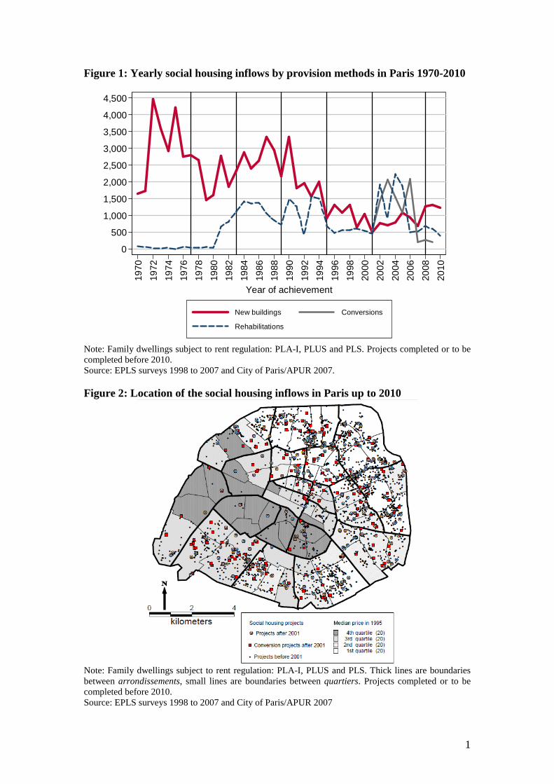
1

Figure 1: Yearly social housing inflows by provision methods in Paris 1970-2010

0

500

1,000

1,500

2,000

2,500

3,000

3,500

4,000

4,500

1970

1972

1974

1976

1978

1980

1982

1984

1986

1988

1990

1992

1994

1996

1998

2000

2002

2004

2006

2008

2010

Year of achievement

New buildings Conversions

Rehabilitations

Note: Family dwellings subject to rent regulation: PLA-I, PLUS and PLS. Projects completed or to be completed before 2010. Source: EPLS surveys 1998 to 2007 and City of Paris/APUR 2007. Figure 2: Location of the social housing inflows in Paris up to 2010

Note: Family dwellings subject to rent regulation: PLA-I, PLUS and PLS. Thick lines are boundaries between arrondissements, small lines are boundaries between quartiers. Projects completed or to be completed before 2010. Source: EPLS surveys 1998 to 2007 and City of Paris/APUR 2007

2

Figure 3: Estimation of the share of social housing in the neighbourhood of a sale

Note: 3 circles (50, 250 and 500 meters), grey dots represent social housing buildings created before 2010. Small lines are IRIS boundaries and the thick line is the boundary between the 13th and 14th arrondissements. Source: EPLS surveys 1998 to 2007 and City of Paris/APUR 2007. Family dwellings subject to rent regulation: PLA-I, PLUS and PLS.

3

Figure 4: Impact of the social housing share on housing prices over time controlling for building unobservables 4.a. Social housing share at 500 meters

-1.50

-1.25

-1.00

-0.75

-0.50

-0.25

0.00

0.25

0.50

0.75

1.00

Impa

ct o

n lo

g h

ousi

ng p

rice

-5 -3 -1 0 1 3 5 7 9 11 13 15Years since projects' completion

Estimate 95% confidence interval

90% confidence interval

4.b. Social housing share at 250 meters

-0.75

-0.50

-0.25

0.00

0.25

0.50

0.75

Impa

ct o

n lo

g h

ousi

ng p

rice

-5 -3 -1 0 1 3 5 7 9 11 13 15Years since projects' completion

Estimate 95% confidence interval

90% confidence interval

Note: The figure represents the impact of the social housing share on housing prices over time including confidence intervals at the 95% level. The zero value on the horizontal axis defines the year in which the first social tenants moved in. The sample includes only the sales between private households occurring within building with repeated sales. Sales’ controls include: a cubic in size, dummy for unknown size, dummies by numbers of rooms interacted with unknown size, dummies for having a bathroom, a parking, a cellar, a lift interacted with the floor of the flat, dummies by periods of construction and a series of quarterly dummies for each quarter from 1995q1 to 2005q4 and quartier linear trends (see appendix table A2). Source: BIEN dataset, DREIF EPLS surveys 1998-2007, City of Paris records. 1999 census at the IRIS (tract) level.

4

Figure 4: Impact of the social housing share on housing prices over time controlling for building unobservables 4.c. Social housing share at 150 meters

-0.25

-0.20

-0.15

-0.10

-0.05

0.00

0.05

0.10

0.15

0.20

0.25

0.30

Impa

ct o

n lo

g h

ousi

ng p

rice

-5 -3 -1 0 1 3 5 7 9 11 13 15Years since projects' completion

Estimate 95% confidence interval

90% confidence interval

4.d. Social housing share at 50 meters

-0.05

-0.03

-0.01

0.01

0.03

0.06

0.08

0.10

0.12

0.14

0.16

Impa

ct o

n lo

g h

ousi

ng p

rice

-5 -3 -1 0 1 3 5 7 9 11 13 15Years since projects' completion

Estimate 95% confidence interval

90% confidence interval

Note: The figure represents the impact of the social housing share on housing prices over time including confidence intervals at the 95% level. The zero value on the horizontal axis defines the year in which the first social tenants moved in. The sample includes only the sales between private households occurring within building with repeated sales. Sales’ controls include: a cubic in size, dummy for unknown size, dummies by numbers of rooms interacted with unknown size, dummies for having a bathroom, a parking, a cellar, a lift interacted with the floor of the flat, dummies by periods of construction and a series of quarterly dummies for each quarter from 1995q1 to 2005q4 and quartier linear trends (see appendix table A2). Source: BIEN dataset, DREIF EPLS surveys 1998-2007, City of Paris records. 1999 census at the IRIS (tract) level.

5

Figure 5: Impact of the social housing share on housing prices over time and by distance belts 5.a. Controlling for building unobservables (350-500 meter belt)

-1.20

-1.00

-0.80

-0.60

-0.40

-0.20

0.00

0.20

0.40

0.60

Impa

ct o

n lo

g h

ousi

ng p

rice

-5 -3 -1 0 1 3 5 7 9 11 13 15Years since projects' completion

Estimate 95% confidence interval

90% confidence interval

5.b. Controlling for building unobservables (50 meter circle)

-0.04

-0.02

0.00

0.02

0.04

0.06

0.08

0.10

0.12

0.14

0.16

Impa

ct o

n lo

g h

ousi

ng p

rice

-5 -3 -1 0 1 3 5 7 9 11 13 15Years since projects' completion

Estimate 95% confidence interval

90% confidence interval

Note: The figure represents the impact of the social housing share on housing prices over time including confidence intervals at the 95% level. The zero value on the horizontal axis defines the year in which the first social tenants moved in. The sample includes only the sales between private households occurring within building with repeated sales. Sales’ controls include: a cubic in size, dummy for unknown size, dummies by numbers of rooms interacted with unknown size, dummies for having a bathroom, a parking, a cellar, a lift interacted with the floor of the flat, dummies by periods of construction and a series of quarterly dummies for each quarter from 1995q1 to 2005q4 and quartier linear trends (see appendix table A2). Source: BIEN dataset, DREIF EPLS surveys 1998-2007, City of Paris records. 1999 census at the IRIS (tract) level.

6

Figure 6: Impact of the social housing share on housing prices over time by neighborhood initial housing prices (50 meters) 6.a. In low-income neighborhoods (1st quartile of housing price in 1995)

-0.05

0.00

0.05

0.10

0.15

0.20

0.25Im

pact

on

log

hou

sing

pri

ce

-5 -3 -1 0 1 3 5 7 9 11 13 15Years since projects' completion

Estimate 95% confidence interval

90% confidence interval

6.b. In high-income neighborhoods (4th quartile of housing price in 1995)

-0.80-0.70-0.60-0.50-0.40-0.30-0.20-0.100.000.100.200.300.400.50

Impa

ct o

n lo

g h

ousi

ng p

rice

-5 -3 -1 0 1 3 5 7 9 11 13 15Years since projects' completion

Estimate 95% confidence interval

90% confidence interval

Note: The figure represents the impact of the social housing share on housing prices over time including confidence intervals at the 95% level. The zero value on the horizontal axis defines the year in which the first social tenants moved in. The sample includes only the sales between private households occurring within building with repeated sales. Sales’ controls include: a cubic in size, dummy for unknown size, dummies by numbers of rooms interacted with unknown size, dummies for having a bathroom, a parking, a cellar, a lift interacted with the floor of the flat, dummies by periods of construction and a series of quarterly dummies for each quarter from 1995q1 to 2005q4 and quartier linear trends (see appendix table A2). Source: BIEN dataset, DREIF EPLS surveys 1998-2007, City of Paris records. 1999 census at the IRIS (tract) level.

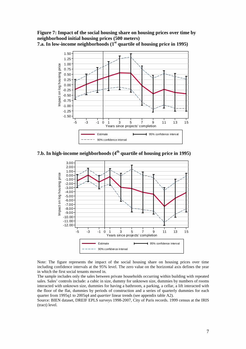
7

Figure 7: Impact of the social housing share on housing prices over time by neighborhood initial housing prices (500 meters) 7.a. In low-income neighborhoods (1st quartile of housing price in 1995)

-1.50

-1.25

-1.00

-0.75

-0.50

-0.25

0.00

0.25

0.50

0.75

1.00

1.25

1.50

Impa

ct o

n lo

g h

ousi

ng p

rice

-5 -3 -1 0 1 3 5 7 9 11 13 15Years since projects' completion

Estimate 95% confidence interval

90% confidence interval

7.b. In high-income neighborhoods (4th quartile of housing price in 1995)

-12.00-11.00-10.00-9.00-8.00-7.00-6.00-5.00-4.00-3.00-2.00-1.000.001.002.003.00

Impa

ct o

n lo

g h

ousi

ng p

rice

-5 -3 -1 0 1 3 5 7 9 11 13 15Years since projects' completion

Estimate 95% confidence interval

90% confidence in terval

Note: The figure represents the impact of the social housing share on housing prices over time including confidence intervals at the 95% level. The zero value on the horizontal axis defines the year in which the first social tenants moved in. The sample includes only the sales between private households occurring within building with repeated sales. Sales’ controls include: a cubic in size, dummy for unknown size, dummies by numbers of rooms interacted with unknown size, dummies for having a bathroom, a parking, a cellar, a lift interacted with the floor of the flat, dummies by periods of construction and a series of quarterly dummies for each quarter from 1995q1 to 2005q4 and quartier linear trends (see appendix table A2). Source: BIEN dataset, DREIF EPLS surveys 1998-2007, City of Paris records. 1999 census at the IRIS (tract) level.

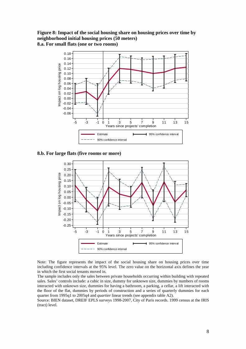
8

Figure 8: Impact of the social housing share on housing prices over time by neighborhood initial housing prices (50 meters) 8.a. For small flats (one or two rooms)

-0.06

-0.04

-0.02

0.000.02

0.04

0.06

0.08

0.10

0.12

0.14

0.16

0.18

Impa

ct o

n lo

g h

ousi

ng p

rice

-5 -3 -1 0 1 3 5 7 9 11 13 15Years since projects' completion

Estimate 95% confidence interval

90% confidence interval

8.b. For large flats (five rooms or more)

-0.25

-0.20

-0.15

-0.10

-0.05

0.00

0.05

0.10

0.15

0.20

0.25

0.30

Impa

ct o

n lo

g h

ousi

ng p

rice

-5 -3 -1 0 1 3 5 7 9 11 13 15Years since projects' completion

Estimate 95% confidence interval

90% confidence interval

Note: The figure represents the impact of the social housing share on housing prices over time including confidence intervals at the 95% level. The zero value on the horizontal axis defines the year in which the first social tenants moved in. The sample includes only the sales between private households occurring within building with repeated sales. Sales’ controls include: a cubic in size, dummy for unknown size, dummies by numbers of rooms interacted with unknown size, dummies for having a bathroom, a parking, a cellar, a lift interacted with the floor of the flat, dummies by periods of construction and a series of quarterly dummies for each quarter from 1995q1 to 2005q4 and quartier linear trends (see appendix table A2). Source: BIEN dataset, DREIF EPLS surveys 1998-2007, City of Paris records. 1999 census at the IRIS (tract) level.

9

Figure 9: Impact of the social housing share on housing prices over time by neighborhood initial housing prices (500 meters) 9.a. For small flats (one or two rooms)

-1.50

-1.25

-1.00

-0.75

-0.50

-0.25

0.00

0.25

0.50

0.75

1.00

1.25

Impa

ct o

n lo

g h

ousi

ng p

rice

-5 -3 -1 0 1 3 5 7 9 11 13 15Years since projects' completion

Estimate 95% confidence interval

90% confidence interval

9.b. For large flats (five rooms or more)

-3.00-2.75-2.50-2.25-2.00-1.75-1.50-1.25-1.00-0.75-0.50-0.250.000.250.500.75

Impa

ct o

n lo

g h

ousi

ng p

rice

-5 -3 -1 0 1 3 5 7 9 11 13 15Years since projects' completion

Estimate 95% confidence interval

90% confidence interval

Note: The figure represents the impact of the social housing share on housing prices over time including confidence intervals at the 95% level. The zero value on the horizontal axis defines the year in which the first social tenants moved in. The sample includes only the sales between private households occurring within building with repeated sales. Sales’ controls include: a cubic in size, dummy for unknown size, dummies by numbers of rooms interacted with unknown size, dummies for having a bathroom, a parking, a cellar, a lift interacted with the floor of the flat, dummies by periods of construction and a series of quarterly dummies for each quarter from 1995q1 to 2005q4 and quartier linear trends (see appendix table A2). Source: BIEN dataset, DREIF EPLS surveys 1998-2007, City of Paris records. 1999 census at the IRIS (tract) level.

10

Table 1: Public and Private dwellings and tenants in Paris in 2002

Social tenants New Social tenants (1) Private tenants Home owners Panel A. Dwelling’s characteristics Mean S.d. Mean S.d. Mean S.d. Mean S.d. Flat size (in m2) 61.80 23.79 58.48 23.41 49.04 32.35 71.19 37.86 Number of rooms 2.90 1.22 2.73 1.20 2.27 1.30 3.22 1.60 Number of dwellings in the building 66.51 81.73 52.25 50.04 32.05 61.35 53.99 113.79 Built before 1914 0.02 0.13 0.02 0.13 0.56 0.50 0.53 0.50 Between 1914 and 49 0.46 0.50 0.51 0.50 0.23 0.42 0.19 0.40 Between 1949 and 81 0.33 0.47 0.15 0.36 0.14 0.35 0.23 0.42 Between 1982 and 90 0.10 0.30 0.12 0.32 0.02 0.15 0.01 0.12 After 1991 0.09 0.29 0.20 0.40 0.05 0.21 0.03 0.18 Monthly rent (euros per m2) 6.17 2.37 6.84 2.48 13.88 6.26 Years of tenancy/ownership 14.28 12.18 2.24 1.13 9.00 12.65 16.82 15.21 Panel B. Household’s characteristics (2) Age 51.81 17.28 39.59 12.52 40.94 16.40 57.05 16.75 Foreign born 0.28 0.45 0.36 0.48 0.27 0.45 0.18 0.38 Couple without children 0.18 0.38 0.12 0.33 0.18 0.38 0.28 0.45 Couple with children 0.21 0.41 0.35 0.48 0.14 0.35 0.16 0.37 Single parents 0.15 0.35 0.19 0.39 0.06 0.23 0.03 0.18 Number of children 0.71 1.21 0.91 1.18 0.35 0.81 0.34 0.79 Without High School dipl. 0.53 0.50 0.48 0.50 0.27 0.44 0.25 0.43 Unemployed (if 18/55 yo) 0.04 0.19 0.07 0.25 0.02 0.15 0.02 0.14 Inactive (if 18/55 yo) 0.09 0.28 0.10 0.30 0.07 0.25 0.08 0.27 Income (euros by Eurostat UC) 16731 8768 15767 8591 24240 20173 32666 23161 Panel C. Building’s maintenance and safety Flood damage last year (flat) 0.19 0.40 0.15 0.35 0.24 0.43 0.22 0.42 Degradation of common space (building) 0.38 0.49 0.26 0.44 0.18 0.38 0.21 0.41 Flat's robbery (or attempt of) 0.22 0.41 0.09 0.28 0.12 0.32 0.13 0.34 Think that neighborhood is not safe 0.23 0.42 0.14 0.34 0.12 0.33 0.15 0.36

Note: (1) New tenants moved in during the last 4 years. (2) For the head of the household. All statistics are weighted using the households’ survey weights. Source: French Housing Survey (ENL) in 2002, Paris.

11

Table 2: Summary statistics. Features of sales and social housing shares in 1995 and 2005 by selected samples

Sample: All buyers and sellers

Buyers and sellers are private households

Buyers and sellers are private households

All sales All sales Repeated sales Within building

(1) (2) (3)

Sold in year: 1995 2005 1995 2005 1995 2005

Mean Mean Mean Mean Mean Mean (s.d.) (s.d.) (s.d.) (s.d.) (s.d.) (s.d.) Panel A. Individual Flat characteristics

Price (euros 2005) 153702 303099 142917 279375 140389 270321 (168283) (301588) (142331) (241548) (133931) (228837) Log price 11.6 12.33 11.56 12.29 11.56 12.27 (0.8) (0.74) (0.75) (0.69) (0.74) (0.68) Price per m2 (euros 2005) 2573.9 5241.3 2520.2 5207.5 2516.4 5165.0 (1043) (1504.5) (859.4) (1340.9) (844) (1308.8) Flat size (in m2) 52.92 54.18 50.95 51.34 50.67 50.22 (34.52) (39.09) (32.06) (34.27) (31.20) (32.77) Missing size 0.48 0.09 0.45 0.08 0.46 0.09 Previous ownership (years) 9.62 9.74 10.61 10.43 10.62 10.44 (9.10) (9.70) (8.80) (9.45) (8.79) (9.45)

Number of rooms

One 0.23 0.24 0.24 0.24 0.24 0.24

Two 0.35 0.34 0.36 0.36 0.37 0.36

Three 0.21 0.21 0.21 0.21 0.21 0.22

Four or more 0.17 0.19 0.16 0.18 0.16 0.17

Unknown 0.03 0.03 0.02 0.02 0.02 0.02

Building age

Before 1914 0.50 0.42 0.53 0.43 0.54 0.46

Between 1914 and 92 0.40 0.46 0.42 0.48 0.42 0.47

After 1992 0.04 0.04 0.00 0.02 0.00 0.01

Unknown 0.05 0.09 0.05 0.07 0.04 0.05

Having at least 1 bathroom 0.77 0.88 0.77 0.88 0.77 0.88

# bathrooms unknown 0.01 0.10 0.01 0.09 0.01 0.09

Having at least 1 parking lot 0.14 0.15 0.11 0.13 0.11 0.14

# parking lots unknown 0.10 0.01 0.10 0.01 0.10 0.01

Panel B. Share of social housing at the time of the sale (by vicinity, circles)

Within 500 meters 0.10 0.12 0.10 0.13 0.10 0.13

(0.10) (0.11) (0.10) (0.11) (0.10) (0.12)

Within 350 meters 0.09 0.12 0.09 0.12 0.09 0.12

(0.11) (0.13) (0.11) (0.13) (0.11) (0.13)

Within 250 meters 0.09 0.11 0.09 0.12 0.09 0.12

(0.13) (0.14) (0.13) (0.14) (0.13) (0.14)

Within 150 meters 0.08 0.10 0.08 0.11 0.08 0.11

(0.18) (0.17) (0.19) (0.17) (0.19) (0.18)

Within 50 meters 0.07 0.09 0.07 0.09 0.07 0.09

(0.46) (0.37) (0.51) (0.38) (0.53) (0.35)

Share of social housing 0.08 0.10 0.08 0.10 0.08 0.11

within the same census tract (0.13) (0.16) (0.13) (0.16) (0.13) (0.16)

# observations 18,437 33,546 12,435 23,686 11,408 20,426

Note: The sample is restricted to the sales between private households for the sets of columns (1) and (2). Source: BIEN dataset, DREIF EPLS surveys 1998-2007, City of Paris records. 1999 census at the IRIS (tract) level.

12

Table 3: Cross sectional estimates of the effects of social housing on housing prices

Dependent variable: ln(price in 2005 euros)

(1) (2) (3) (4) (5) Vicinity of the sales, within: 500 meters 250 meters 150 meters 50 meters Census

tract Panel A. Years 1995 to 2005 without flat’s controls

Share of social housing -1.404*** -0.883*** -0.474*** -0.066*** -0.667***

(0.101) (0.081) (0.078) (0.024) (0.069)

Variation in the last 10 years -7.440*** -2.883*** -1.075*** -0.113** -1.574***

(0.505) (0.359) (0.297) (0.045) (0.240)

Variation in the next 5 years -7.092*** -2.282*** -1.105*** -0.263*** -0.922**

(0.742) (0.435) (0.309) (0.070) (0.375) Year times quarter dummies Yes Yes Yes Yes Yes

Flat’s controls No No No No No Panel B. Years 1995 to 2005 with flat’s controls

Share of social housing -1.152*** -0.735*** -0.376*** -0.051*** -0.557***

(0.058) (0.047) (0.053) (0.019) (0.038)

Variation in the last 10 years -5.576*** -2.190*** -0.806*** -0.076** -1.165***

(0.276) (0.224) (0.198) (0.031) (0.129)

Variation in the next 5 years -5.168*** -1.959*** -0.894*** -0.143*** -0.887***

(0.431) (0.255) (0.166) (0.034) (0.213) Year times quarter dummies Yes Yes Yes Yes Yes

Flat’s controls Yes Yes Yes Yes Yes

# observations 208,918 208,918 208,918 208,918 208,918 # clusters 902 902 902 902 902

Note: Each cell is from a different OLS regression. * significant at the 10% level, ** at 5%, *** at 1%. Standard errors are clustered by census tract (IRIS). In panel B, a basic set of flat’s and sales’ controls is included in all the regressions. Sales’ controls include: a cubic in size, dummy for unknown size, dummies by numbers of rooms interacted with unknown size, dummies for having a bathroom, a parking, a cellar, a lift interacted with the floor of the flat, dummies by periods of construction (see appendix table A2). The variation in the last ten years of this measure corresponds to the change between 1985 and 1995 for year 1995. The variation in the next five years of this measure corresponds to the change between 1995 and 2000 for year 1995. Source: BIEN dataset, DREIF EPLS surveys 1998-2007, City of Paris records. 1999 census at the IRIS (tract) level. The sample includes only the sales between private households occurring within building with repeated sales.

13

Table 4. Estimates of the effects of social housing on housing prices with alternative geographical controls

Dependent variable: ln (price in euros 2005)

Vicinity of the sales, within: 500 meters 250 meters 150 meters 50 meters

Panel A. Estimates without control for different price trends around the sales

(1) (2) (3) (4) (5) (6) (7) (8) (9) (10) (11) (12)

Share of social -0.603*** -0.276*** 0.301* -0.307*** -0.113*** 0.107 -0.132*** -0.046*** 0.088 -0.016*** -0.003 0.064*** housing (0.044) (0.046) (0.177) (0.027) (0.018) (0.099) (0.019) (0.010) (0.057) (0.005) (0.002) (0.018) R-squared 0.863 0.871 0.911 0.862 0.871 0.911 0.861 0.871 0.911 0.860 0.871 0.911

Fixed effects Quartier Tract Building Quartier Tract Building Quartier Tract Building Quartier Tract Building

Quartiers trends No No No No No No No No No No No No

Sales controls Yes Yes Yes Yes Yes Yes Yes Yes Yes Yes Yes Yes

Panel B. Estimates controlling for different price trends around the sales

(1) (2) (3) (4) (5) (6) (7) (8) (9) (10) (11) (12)

Share of social -0.608*** -0.304*** 0.157 -0.308*** -0.116*** 0.097 -0.132*** -0.047*** 0.081** -0.016*** -0.003 0.058*** housing (0.044) (0.045) (0.139) (0.027) (0.018) (0.071) (0.019) (0.010) (0.041) (0.005) (0.002) (0.016) R-squared 0.864 0.872 0.912 0.863 0.872 0.912 0.862 0.872 0.912 0.862 0.872 0.912

Fixed effects Quartier Tract Building Quartier Tract Building Quartier Tract Building Quartier Tract Building

Quartiers trends Yes Yes Yes Yes Yes Yes Yes Yes Yes Yes Yes Yes

Sales controls Yes Yes Yes Yes Yes Yes Yes Yes Yes Yes Yes Yes

# observations 208,918 208,918 208,918 208,918 208,918 208,918 208,918 208,918 208,918 208,918 208,918 208,918

# clusters 902 902 902 902 902 902 902 902 902 902 902 902

Note: * significant at the 10% level, ** at 5%, *** at 1%. Standard errors are clustered at the census tract level. The sample includes only the sales between private households within buildings with repeated sales. Sales’ controls include: a cubic in size, dummy for unknown size, dummies by numbers of rooms interacted with unknown size, dummies for having a bathroom, a parking, a cellar, a lift interacted with the floor of the flat, dummies by periods of construction and a series of quarterly dummies for each quarter from 1995q1 to 2005q4 (see appendix table A2). Source: BIEN dataset, DREIF EPLS surveys 1998-2007, City of Paris records. 1999 census at the IRIS (tract) level.

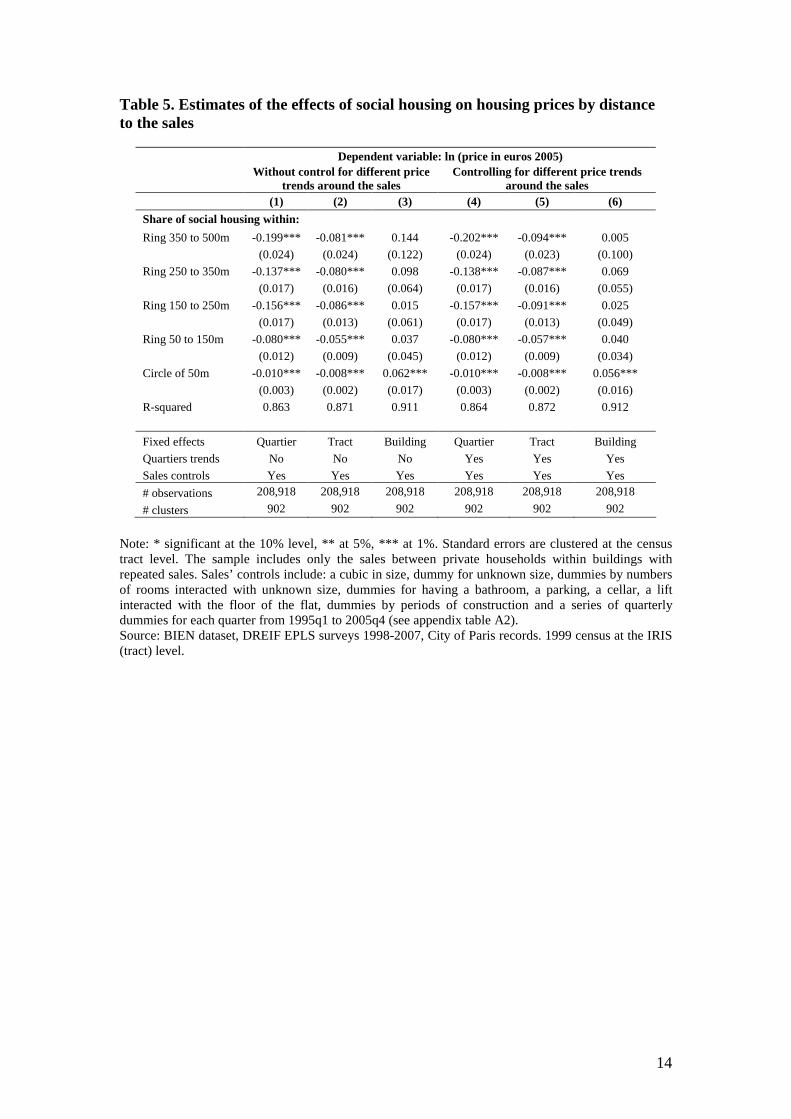
14

Table 5. Estimates of the effects of social housing on housing prices by distance to the sales

Dependent variable: ln (price in euros 2005)

Without control for different price

trends around the sales Controlling for different price trends

around the sales

(1) (2) (3) (4) (5) (6)

Share of social housing within:

Ring 350 to 500m -0.199*** -0.081*** 0.144 -0.202*** -0.094*** 0.005

(0.024) (0.024) (0.122) (0.024) (0.023) (0.100)

Ring 250 to 350m -0.137*** -0.080*** 0.098 -0.138*** -0.087*** 0.069

(0.017) (0.016) (0.064) (0.017) (0.016) (0.055)

Ring 150 to 250m -0.156*** -0.086*** 0.015 -0.157*** -0.091*** 0.025

(0.017) (0.013) (0.061) (0.017) (0.013) (0.049)

Ring 50 to 150m -0.080*** -0.055*** 0.037 -0.080*** -0.057*** 0.040

(0.012) (0.009) (0.045) (0.012) (0.009) (0.034)

Circle of 50m -0.010*** -0.008*** 0.062*** -0.010*** -0.008*** 0.056***

(0.003) (0.002) (0.017) (0.003) (0.002) (0.016)

R-squared 0.863 0.871 0.911 0.864 0.872 0.912

Fixed effects Quartier Tract Building Quartier Tract Building

Quartiers trends No No No Yes Yes Yes

Sales controls Yes Yes Yes Yes Yes Yes

# observations 208,918 208,918 208,918 208,918 208,918 208,918

# clusters 902 902 902 902 902 902

Note: * significant at the 10% level, ** at 5%, *** at 1%. Standard errors are clustered at the census tract level. The sample includes only the sales between private households within buildings with repeated sales. Sales’ controls include: a cubic in size, dummy for unknown size, dummies by numbers of rooms interacted with unknown size, dummies for having a bathroom, a parking, a cellar, a lift interacted with the floor of the flat, dummies by periods of construction and a series of quarterly dummies for each quarter from 1995q1 to 2005q4 (see appendix table A2). Source: BIEN dataset, DREIF EPLS surveys 1998-2007, City of Paris records. 1999 census at the IRIS (tract) level.

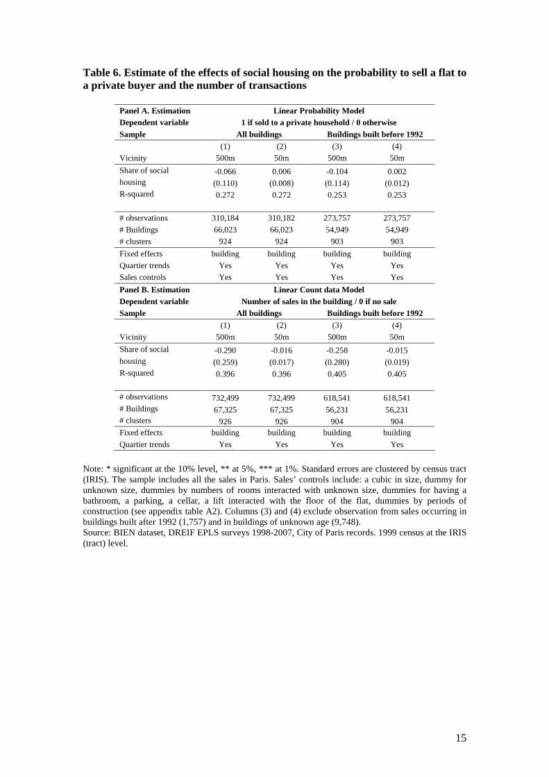
15

Table 6. Estimate of the effects of social housing on the probability to sell a flat to a private buyer and the number of transactions

Panel A. Estimation Linear Probability Model Dependent variable 1 if sold to a private household / 0 otherwise Sample All buildings Buildings built before 1992

(1) (2) (3) (4)

Vicinity 500m 50m 500m 50m

Share of social -0.066 0.006 -0.104 0.002 housing (0.110) (0.008) (0.114) (0.012) R-squared 0.272 0.272 0.253 0.253

# observations 310,184 310,182 273,757 273,757

# Buildings 66,023 66,023 54,949 54,949

# clusters 924 924 903 903

Fixed effects building building building building

Quartier trends Yes Yes Yes Yes

Sales controls Yes Yes Yes Yes

Panel B. Estimation Linear Count data Model Dependent variable Number of sales in the building / 0 if no sale Sample All buildings Buildings built before 1992 (1) (2) (3) (4)

Vicinity 500m 50m 500m 50m

Share of social -0.290 -0.016 -0.258 -0.015 housing (0.259) (0.017) (0.280) (0.019) R-squared 0.396 0.396 0.405 0.405

# observations 732,499 732,499 618,541 618,541 # Buildings 67,325 67,325 56,231 56,231 # clusters 926 926 904 904 Fixed effects building building building building

Quartier trends Yes Yes Yes Yes

Note: * significant at the 10% level, ** at 5%, *** at 1%. Standard errors are clustered by census tract (IRIS). The sample includes all the sales in Paris. Sales’ controls include: a cubic in size, dummy for unknown size, dummies by numbers of rooms interacted with unknown size, dummies for having a bathroom, a parking, a cellar, a lift interacted with the floor of the flat, dummies by periods of construction (see appendix table A2). Columns (3) and (4) exclude observation from sales occurring in buildings built after 1992 (1,757) and in buildings of unknown age (9,748). Source: BIEN dataset, DREIF EPLS surveys 1998-2007, City of Paris records. 1999 census at the IRIS (tract) level.

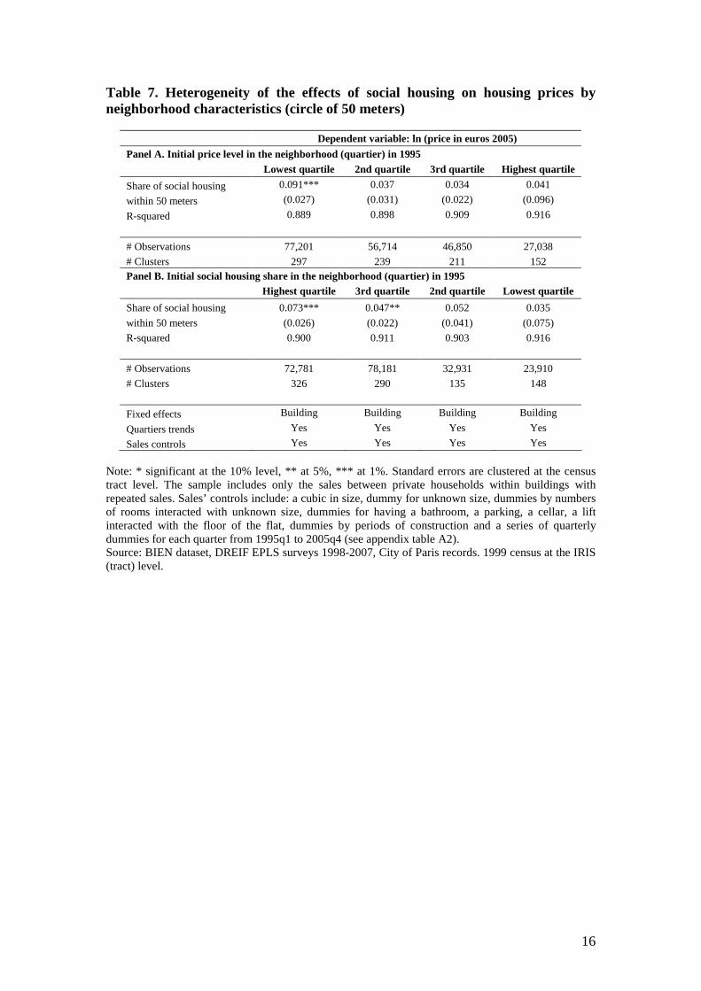
16

Table 7. Heterogeneity of the effects of social housing on housing prices by neighborhood characteristics (circle of 50 meters)

Dependent variable: ln (price in euros 2005)

Panel A. Initial price level in the neighborhood (quartier) in 1995

Lowest quartile 2nd quartile 3rd quartile Highest quartile

Share of social housing 0.091*** 0.037 0.034 0.041

within 50 meters (0.027) (0.031) (0.022) (0.096)

R-squared 0.889 0.898 0.909 0.916

# Observations 77,201 56,714 46,850 27,038

# Clusters 297 239 211 152 Panel B. Initial social housing share in the neighborhood (quartier) in 1995

Highest quartile 3rd quartile 2nd quartile Lowest quartile

Share of social housing 0.073*** 0.047** 0.052 0.035

within 50 meters (0.026) (0.022) (0.041) (0.075)

R-squared 0.900 0.911 0.903 0.916

# Observations 72,781 78,181 32,931 23,910

# Clusters 326 290 135 148

Fixed effects Building Building Building Building Quartiers trends Yes Yes Yes Yes

Sales controls Yes Yes Yes Yes

Note: * significant at the 10% level, ** at 5%, *** at 1%. Standard errors are clustered at the census tract level. The sample includes only the sales between private households within buildings with repeated sales. Sales’ controls include: a cubic in size, dummy for unknown size, dummies by numbers of rooms interacted with unknown size, dummies for having a bathroom, a parking, a cellar, a lift interacted with the floor of the flat, dummies by periods of construction and a series of quarterly dummies for each quarter from 1995q1 to 2005q4 (see appendix table A2). Source: BIEN dataset, DREIF EPLS surveys 1998-2007, City of Paris records. 1999 census at the IRIS (tract) level.

17

Table 8. Heterogeneity of the effects of social housing on housing prices by neighborhood characteristics (circle of 500 meters)

Dependent variable: ln (price in euros 2005)

Panel A. Initial price level in the neighborhood (quartier) in 1995

Lowest quartile 2nd quartile 3rd quartile Highest quartile

Share of social housing 0.202 0.089 0.000 -0.120

within 500 meters (0.263) (0.233) (0.194) (0.871)

R-squared 0.889 0.898 0.909 0.916

# Observations 77,201 56,714 46,850 27,038

# Clusters 297 239 211 152 Panel B. Initial social housing share in the neighborhood (quartier) in 1995

Highest quartile 3rd quartile 2nd quartile Lowest quartile

Share of social housing 0.026 -0.030 1.417*** -1.331

within 500 meters (0.192) (0.193) (0.535) (0.993)

R-squared 0.900 0.911 0.903 0.916

# Observations 72,781 78,181 32,931 23,910

# Clusters 326 290 135 148

Fixed effects Building Building Building Building Quartiers trends Yes Yes Yes Yes

Sales controls Yes Yes Yes Yes

Note: * significant at the 10% level, ** at 5%, *** at 1%. Standard errors are clustered at the census tract level. The sample includes only the sales between private households within buildings with repeated sales. Sales’ controls include: a cubic in size, dummy for unknown size, dummies by numbers of rooms interacted with unknown size, dummies for having a bathroom, a parking, a cellar, a lift interacted with the floor of the flat, dummies by periods of construction and a series of quarterly dummies for each quarter from 1995q1 to 2005q4 (see appendix table A2). Source: BIEN dataset, DREIF EPLS surveys 1998-2007, City of Paris records. 1999 census at the IRIS (tract) level.

18

Table 9. Heterogeneity of the effects of social housing on housing prices by flats’ characteristics (circles of 500 and 50 meters)

Dependent variable: ln (price in euros 2005)

Share of social housing within 500 meters within 50 meters Interacted with: (1) (2) (3) (4) No variable 0.600*** 0.082*** (0.136) (0.019) Number of rooms is 1 or 2 0.299** 0.065*** (0.136) (0.016) Number of rooms is 3 or 4 -0.022 0.051***

(0.140) (0.016)

Number of rooms is greater than 4 -0.417*** 0.008

(0.142) (0.018)

Number of rooms -0.190*** -0.010** (0.012) (0.005) Number of rooms is unknown 0.362* -0.245** 0.060 -0.022 (0.190) (0.123) (0.053) (0.053) R-squared 0.912 0.912 0.912 0.912 Fixed effects Building Building Building Building Quartiers trends Yes Yes Yes Yes Sales controls Yes Yes Yes Yes

# Observations 208,918 208,918 208,918 208,918

# Clusters 902 902 902 902

Note: * significant at the 10% level, ** at 5%, *** at 1%. Standard errors are clustered at the census tract level. The sample includes only the sales between private households within buildings with repeated sales. Sales’ controls include: a cubic in size, dummy for unknown size, dummies by numbers of rooms interacted with unknown size, dummies for having a bathroom, a parking, a cellar, a lift interacted with the floor of the flat, dummies by periods of construction and a series of quarterly dummies for each quarter from 1995q1 to 2005q4 (see appendix table A2). Source: BIEN dataset, DREIF EPLS surveys 1998-2007, City of Paris records. 1999 census at the IRIS (tract) level.

19

Table 10: Estimates of the effects of the conversion projects on housing prices

Dependent variable: ln(price in 2005 euros)

(1) (2) (3) (4) Vicinity of the sales, within: 500 meters 250 meters 150 meters 50 meters

Panel A. Effect of the conversion projects

Share of conversion projects -0.314 -0.055 0.023 0.032

(0.340) (0.135) (0.066) (0.033)

R-squared 0.924 0.924 0.924 0.924

# observations 116,105 116,105 116,105 116,105 # clusters 892 892 892 892 Panel B. Controlling for the share of other social housing projects

Share of conversion projects -0.510 -0.122 -0.062 0.017

(0.354) (0.142) (0.074) (0.034)

Share of other projects 0.500** 0.186 0.201** 0.055*

(0.232) (0.115) (0.080) (0.030)

R-squared 0.924 0.924 0.924 0.924

# observations 116,105 116,105 116,105 116,105 # clusters 892 892 892 892 Fixed effects Building Building Building Building Quartiers trends Yes Yes Yes Yes

Sales controls Yes Yes Yes Yes

Note: * significant at the 10% level, ** at 5%, *** at 1%. Standard errors are clustered by census tract (IRIS). The sample includes only the sales between private households occurring within building with repeated sales. Sales’ controls include: a cubic in size, dummy for unknown size, dummies by numbers of rooms interacted with unknown size, dummies for having a bathroom, a parking, a cellar, a lift interacted with the floor of the flat, dummies by periods of construction (see appendix table A2). Source: BIEN dataset, DREIF EPLS surveys 1998-2007, City of Paris records. 1999 census at the IRIS (tract) level.

20

Appendices Figure A1: Housing prices per square meters in Paris in 1995 by quartiers

Note: The sample includes only the sales between private households in 1995 with information about price and surface. Thick lines represent the boundaries of the 20 arrondissements. Source: BIEN dataset. Figure A2: Social housing share in Paris in 1995 by quartiers

Note: Thick lines represent the boundaries of the 20 arrondissements. Source: DREIF EPLS surveys 1998-2007 and 1999 census.

21

Table A1: Summary statistics. Social housing share for the sample of sales 1995-2005 by circles and belts

Year 1995 2005 1995-2005 1995 2005 1995-

2005

Mean Mean Mean Mean Mean Mean

(s.d.) (s.d.) (s.d.) (s.d.) (s.d.) (s.d.)

Vicinity Within circles Vicinity Within belts

500 m 0.10 0.13 0.11 350-500 m 0.10 0.13 0.12

(0.10) (0.12) (0.11) (0.11) (0.13) (0.12)

350 m 0.09 0.12 0.11 250-350 m 0.10 0.13 0.12

(0.11) (0.13) (0.12) (0.13) (0.15) (0.14)

250 m 0.09 0.12 0.10 150-250 m 0.09 0.12 0.11

(0.13) (0.14) (0.13) (0.14) (0.16) (0.15)

150 m 0.08 0.11 0.09 50-150 m 0.08 0.11 0.10

(0.19) (0.18) (0.18) (0.20) (0.19) (0.18)

50 m 0.07 0.09 0.08 50 m 0.07 0.09 0.08

(0.53) (0.35) (0.49) (0.53) (0.35) (0.49)

Within census 0.08 0.11 0.09 Within census 0.08 0.11 0.09

tract (0.13) (0.16) (0.14) tract (0.13) (0.16) (0.14)

# observations 11,408 20,426 208,918 11,408 20,426 208,918

Note: The sample is restricted to the sales between private households within buildings with repeated sales. Source: BIEN dataset, DREIF EPLS surveys 1998-2007, City of Paris records. 1999 census at the IRIS (tract) level.

22

Table A2: Summary statistics. Characteristics of the repeated sales within buildings

Variable Mean (Std. Dev.) Price (euros 2005) 173,650.9 (173,133.1) Log (price) 11.743 (0.784) 1 room 0.236 2 rooms 0.367 3 rooms 0.219 4 rooms 0.101 5 rooms or more 0.060 Number of rooms unknown 0.017 1 room and unknown flat size 0.054 2 rooms and unknown flat size 0.084 3 rooms and unknown flat size 0.050 4 rooms and unknown flat size 0.024 5 rooms or more and unknown flat size 0.016 Rooms and flat size unknown 0.007 Flat size (0 if unknown) 38.274 (35.445) Flat size squared/100 27.212 (58.153) Flat size cubed/10000 27.941 (147.307) Flat size unknown 0.235 At least one bathroom 0.825 Number of bathrooms unknown 0.032 At least one parking space 0.126 Number of parking spaces unknown 0.140 Having a lift 0.458 Having a cellar 0.715 Ground floor 0.079 1st floor 0.152 2nd floor 0.161 3rd floor 0.157 4th floor or higher 0.435 Floor unknown 0.016 1st floor and lift 0.059 2nd floor and lift 0.063 3rd floor and lift 0.063 4th floor or higher and lift 0.060 Floor unknown and lift 0.007 Period of construction 1850 or before 0.053 1850 / 1913 0.454 1914 / 1947 0.157 1948 / 1969 0.136 1970 / 1980 0.123 1981 / 1991 0.018 1992 / 2000 0.008 After 2001 0.001 Unknown 0.050 # observations 208,918

Note: The sample is restricted to the sales between private households within buildings with repeated sales. Source: BIEN dataset.