the external finance premium in brazil: empirical … · analyses using state space models fernando...

THE EXTERNAL FINANCE PREMIUM IN BRAZIL: EMPIRICAL

ANALYSES USING STATE SPACE MODELS

FERNANDO NASCIMENTO DE OLIVEIRA

(CENTRAL BANK OF BRAZIL)12

ABSTRACT

Our objective in this paper is to estimate the external finance premium (EFP), which is a

non observable variable, of firms in Brazil using state space models. For this purpose,

we built an original database with confidential and public data containing balance sheet

information of 5,026 public and private firms from the third quarter of 1994 to the

fourth quarter of 2010. Our results show that the average and volatility of the EFP of

small firms is higher than those of large firms and that the EFP is more sensitive to

monetary policy for small firms than for large firms. We also found that the sensitivity

in relation to EFP of inventories, short term debt and net operational revenues, all in

proportion of total assets is higher for small firms than for large firms. These empirical

evidences point to the importance of the balance sheet channel of the transmission

mechanism of monetary policy in Brazil.

Key Words: External Finance Premium (EFP), State Space Models, Kalman Filter,

Monetary Transmission Mechanism, Balance Sheet Channel.

JEL G30, G32

1 Research Department Rio de Janeiro

2 We thank Eduardo Klumb (IBMEC/RJ) and Alberto Ronchi (Previ S/A) for research assistance. I am

especially thankful of Eduardo Klumb for obtaining the SERASA database and making it available for

this paper. We also thank INSPER/SP for making the Gazeta Mercantil database also available for this

paper. Both SERASA and Gazeta Mercantil database are confidential.

2

1-Introduction

The external finance premium (EFP), defined as the difference between the cost of

raising funds externally and the opportunity cost of internal funds, is a fundamental

variable in economics. While internal finance is available relatively cheaply, obtaining

external funds through loans, bonds or equity possibly implies substantial costs.

The EFP is a crucial variable to understand several microeconomic decisions of firms,

such as capital structure, dividend and compensation policies, demand for investment

among others. It is also important in a macroeconomic context because it is the key

variable related to the credit channels of monetary transmission mechanisms, such as

the bank lending and balance sheet channel.34

3 Credit channel theories can be broken down into two distinct theories: the bank lending and the balance

sheet theories. In the former, monetary contractions increase the adverse selection problems between

firms and banks, which may decrease the volumes of loans from banks to firms and households. The

reason for this is that banks experience a decrease in the volume of demand deposits that can lead to a

decrease in the volumes of loans if they are not able to replace demand deposits with other financial

instruments. The balance sheet channel of monetary policy arises because policy shifts affect not only

market interest rates, but also the borrowers’ financial positions, both directly and indirectly. A tight

monetary policy directly weakens borrowers’ balance sheets in at least two ways. First, a rise in interest

rates directly increases interest expenses, reducing net cash flows and weakening the borrowers’ financial

position. Second, a rise in interest rates is also typically associated with declining asset prices, which,

among other things, shrink the value of the borrowers’ collateral. In the aggregate, these effects could

lead to a substantial impact on aggregate demand.

4 The credit channel considers the existence of a financial premium, that is a difference between the cost

of funds raised externally (issued by equity or debt) and the opportunity costs of funds raised internally

(by retaining earnings). The size of the external finance premium reflects imperfections in credit markets.

The explanation of the dynamics of this premium can improve the timing and strength of monetary policy

provided by traditional mechanism. The credit view as a whole is interesting and important for several

reasons. First, if the credit view is correct, it means that monetary policy can affect the real economy

without much variation in the open-market interest rates. Second, the view can explain how monetary

contraction influences investment and inventory behavior. Finally, the credit view also implies that the

impact of monetary policy on economic activity is not always the same. It is also sensitive to the state of

firms’ balance sheet and health of the banking sector.

3

However, as Bernanke and Gertler (1995) discuss a major problem for empirical studies

in this area is that the EFP is a non observable variable. There are currently two

approaches that tackle this fact. 5

The first approach relies on finding readily available financial market indicators that are

arguably good indicators for the EFP, such as corporate bond spreads for instance. The

fact that these indicators have substantial predictive content for business cycle

fluctuations is often interpreted as evidence for the existence of financial frictions, as

Gertler and Lown (1999) and Mody and Taylor (2003) argue. Another approach is

adopted by Levin et al. (2004) that use microeconomic financial frictions along with

balance sheet and bond market data, to estimate the external finance premium for a

group of listed firms in the USA. 6

In this paper, we contribute to the literature by taking a different approach to estimate

the EFP. We estimate it for Brazilian private and public firms using a state space

framework. The EFP for each one of the firms in our database is a smooth Kalman filter

of the state variable. In our estimation of the state space model, we use several signal

and control variables related to financial indicators of the firms highly correlated with

credit market imperfections.

To achieve our objectives, we use an original and confidential database composed of

unbalanced balance sheet information of 291 public firms and 4,735 private firms. Of

the private firms, 102 disclose quarterly information while all the others disclose only

end of the year information.7 The information of the public firms comes from Comissão

de Valores Imobiliários (CVM) and Economatica and the information of the private

firms come from Valor Econômico and from confidential data of SERASA and Gazeta

Mercantil. 89

5 Bernanke and Gertler (1995) use the inverse of coverage ratio.

6 There is a vast empirical literature that uses one or these approaches. See Grave (2008) for a good

discussion about this literature and about the EFP in the USA. 7 All public corporations disclose quarterly balance sheet information. We use their consolidated balance

sheet information. 8 SERASA is a privately held company that has one of the largest databases of financial and accounting

information of firms and individuals in the world. The data is related to debt of firms and individuals in

Brazil. The information of SERASA is provided to banks, to trade shops, small, medium and large

4

We choose size defined as total assets as our criteria to classify firms in small or large.

We verify that size is highly correlated to other financial characteristics of firms that

indicate the degree in which firms access the financial markets.

Our results show that small firms in Brazil have a much higher average as well as

volatility of EFP than large firms. The EFP of small firms is much more elastic to the

interest rate than the EFP of large firms. We also find that the elasticity of inventories,

short term debt and net operational revenues all as a proportion of total assets relative to

EFP is higher for small firms than large firms. Finally, we have empirical evidence that

these elasticities decrease in the case the firm had an outstanding loan with Brazil’s

development bank, Banco Nacional de Desenvolvimento Social (BNDES), in our

sample period. Our results seem robust to different specifications of the state space

models. Therefore, these results seem to indicate the relevance of the balance sheet

explanation of the monetary transmission mechanism in Brazil.

Brazil is a very special case of an emerging market where asymmetries of information

could play a very important role in the transmission mechanism of monetary policy.

Brazil has a very interesting financial system. In some of its aspects, like its means of

payments, for instance, the Brazilian financial system rivals that of developed countries.

However, as far as volume of credit to households and firms and depth of the capital

markets is considered, Brazil still lags behind OECD countries.10

The cost of capital in Brazil is very high when compared to international standards. The

spread banks charge on their loans, even for very well rated companies, is well above

companies, with the goal of giving support to credit decisions and thus make business more cheap, fast

and reliable. The data from SERASA goes from 1998 to 2007, and is both quarterly and annual.

9 The data of Gazeta Mercantil is annual and goes from 1998 to 2007 and is based on the balance sheet

information of private firms published in this newspaper. The information of Valor Econômico is annual

and goes from 2009 to 2010 and is based on the balance sheet information available on the 1000 Maiores

Empresas publication. 10

The total credit to the private sector is around 50% of GNP, while in the USA, for example, it is over

100% of GNP.

5

what is charged worldwide. This high cost of capital creates enormous agency costs

between private agents and financial institutions.11

Another very important characteristic of corporations in Brazil is that, due to the high

costs of capital, many of them look for a public development bank (BNDES - Brazilian

Social and Economic Development Bank)- for long-term financing. Not only are

interest rates much lower, but also maturities are much longer. Monetary policy affects

only indirectly the long-term interest rates set by the BNDES in its loans.

There is a vast literature both empirical and theoretical about EFP. Most papers focus on

the macroeconomic aspects of EFP. Just to cite some empirical papers, we could point

to Gertler and Gilchrist (1994) that use the inverse of coverage ratio as a proxy for EFP

of firms in United States. Gertler and Gilchrist conclude that balance sheet effects can

be more relevant for smaller firms (defined by the relative size of its total assets in

relation to large firms).

Oliveira (2009) undertakes a similar work to Gertler e Gilchrist (1994) for Brazil

adopting also the firm’s size as a measure of credit market access. The empirical

analyses were conducted over a database of public firms between the third quarter of

1994 and the fourth quarter of 2007. Following Gertler and Gilchrist (1994), Oliveira

concludes that smaller firms are more sensitive to EFP than large firms.

Gilchrist and Himmelberg (1995, 1998) investigate the influence of fundamental

(expected return and present value) and financial (availability of internal and external

funds) factors on firms investment decisions considering capital market imperfections.

Among others characteristics, the authors adopted the existence of debt rating as a

criterion to measure the credit market imperfections. According to the authors,

considering that most companies that issues public debt obtains a bond rating, this

strategy permits to split the sample into firms that have, or not, issued public debt in the

past. If the company didn’t issue debt it must have faced more constraints in credit

11

This is how the literature defines credit market imperfections in general terms.

6

market access. Their empirical analyses indicated that non rating firms are more

sensitive to EFP than large firms.

The rest of this paper is organized as follows. Section 2 describes the data. Section 3

presents our model. Section 4 presents the empirical analyses. Section 5 concludes.

2. Data

We built an original and confidential database of an unbalanced panel of balance sheet

information of 291 public firms and 4,735 private firms from the third quarter of 1994

to the fourth quarter of 2010. Of the private firms, 102 disclose quarterly information

while all the others disclose only end of the year information.12

The information of the

public firms comes from Comissão de Valores Imobiliários (CVM) and Economatica

and, and the information of the private firms come from Valor Econômico and

confidential data of SERASA and Gazeta Mercantil.

We take size, measured by total assets, as our classification criteria for credit access

following Gertler and Gilchrist (1994). We observe that size is highly correlated with

other financial variables that indicate the capacity firms have to access the financial

markets. We classify firms into small and large. We will show that our small firms have

relatively less access to the financial markets than do large corporations.

Our interest in separating firms into large and small ones is that, as Gertler and Gilchrist

(1994) point out, is that by doing this we can infer the level of access of the firms to the

financial markets. In theory, small firms will depend much more on bank loans than will

large firms. The latter will also issue much more short-term and long-term debts and

will have more inventories.

In the case of firms with quarterly information, we consider a possible candidate for

small firm one whose logarithm of total assets is less than or equal to the 30th percentile

of the distribution of total assets in at least one quarter of our sampling periods. In a

12

All public corporations disclose quarterly balance sheet information. We use their consolidated balance

sheet information.

7

similar fashion, we consider a possible candidate for large firm, one whose logarithm of

total assets is greater than or equal to the 30th percentile in at least one year of our

sampling periods. Thus, we obtain 112 small firms and 68 large firms. Of the 68 large

firms, five are private ones. Of the 112 small firms, 36 are private ones.

In the case of firms with yearly information, we consider a firm to be small if its

logarithm of total assets is less than or equal to the 30th percentile in at least one year. A

firm is large if its logarithm of total assets is greater than or equal to the 70th percentile

in at least one year. Thus, we obtain 108 large firms and 181 small firms.

We look at the skewness of the distribution of small and large firms in every quarter or

year. We could have problems in our sample selection if the distribution of small firms

were skewed to the right or if the distribution of large firms were skewed to the left.

This could indicate that our cut-off for small and large is not a good one. The averages

of quarterly skewness (considering all periods) were 0.89 and 1.59 for small and large

firms, respectively. In the case of end-of-the-year information, the skewness

(considering all periods) was 0.79 for small firms and 1.21 for large firms. These results

indicate that our classification scheme is not a bad one as far as the cut-off is concerned.

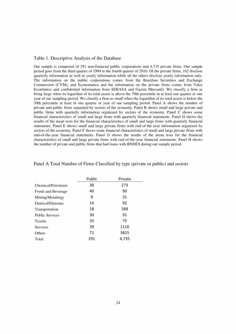
Panel A of Table 1 shows all firms, private and public, classified by sectors of the

economy. As one can see, public firms come mostly from the food and beverages

sector (13.74%), while private firms come mostly from the services sector (23.44%).

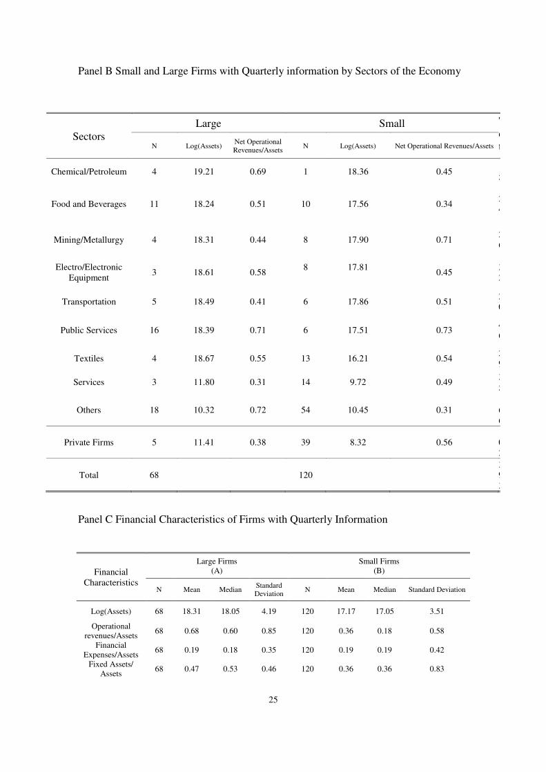
Panel B of Table 1 shows the small and large public and private firms with quarterly

information organized by the sector of the economy they belong to. As one would

imagine, large firms (23%) include concessionaries of public services, followed by the

food and beverage sector (16%) while small firms include mostly the service sector

(11%) followed by the textile sector (11%).

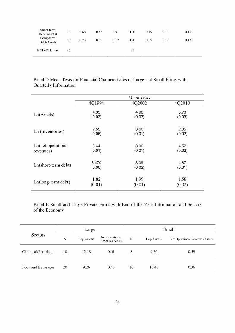
Panel C of Table 1 presents the mean values of some financial characteristics of small

and large firms for the whole sample relative to their assets. As we can easily verify,

large firms have, on average, greater long-term and short-term debt than do small firms.

Large firms also have more fixed assets and net operational revenues as a percentage of

8

total assets. Finally, 53% of large firms (36 firms) have much more outstanding loans

with the BNDES compared to only 18.0% of small firms (22 firms).

Panel D of Table 1 shows some mean tests for these characteristics considering the

financial statements of the last quarters of the years 1999, 2002 and 2010. As one can

see, all p-values of the differences in the mean values for the characteristics between

large and small firms are close to 0. Therefore, it seems that small firms in our sample

of quarterly data differ from large firms as far as access to the financial market is

concerned. They have less access to the financial markets.

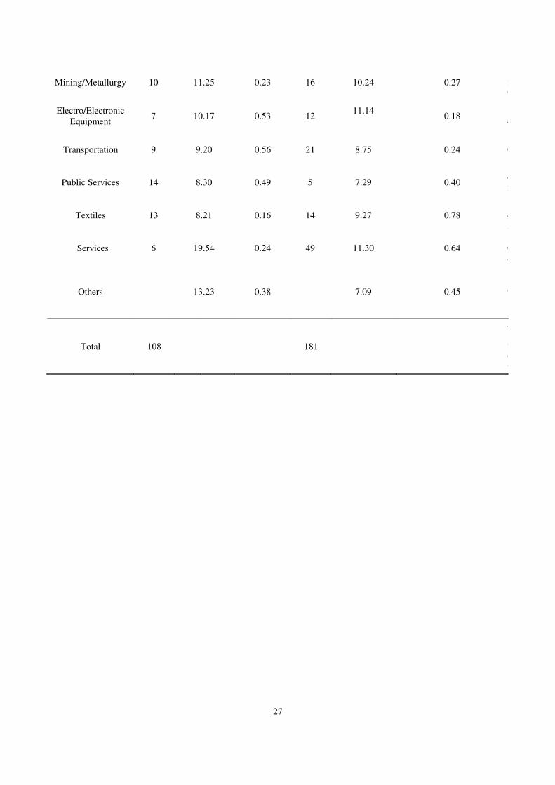
Panel E of Table 1 shows the small and large private firms with end-of-the-year

information organized by the sector of the economy they belong to. We have 4,735 non-

financial firms in our database with balance sheet information for all years from 1998 to

2007. There are 108 large firms and 181 small firms. Of the large firms, 18% pertain to

the food and beverage sector. In the case of small private firms, 26% belong to the

service sector.

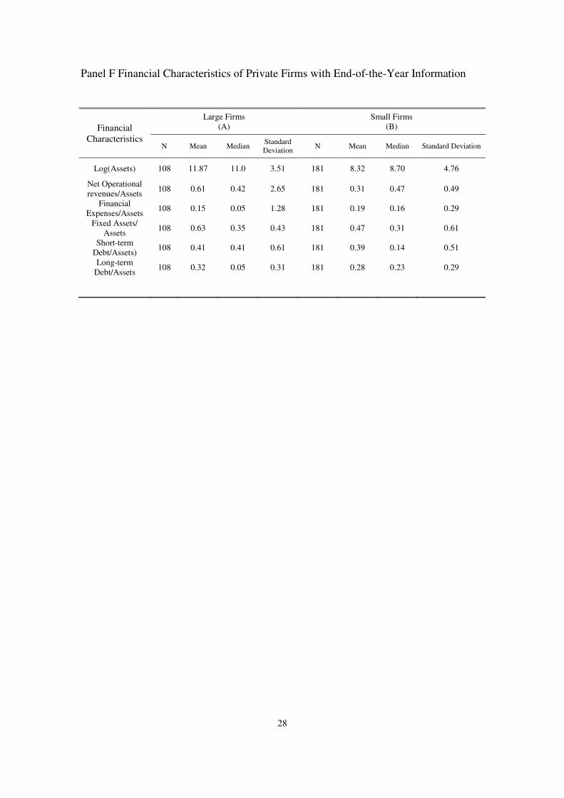
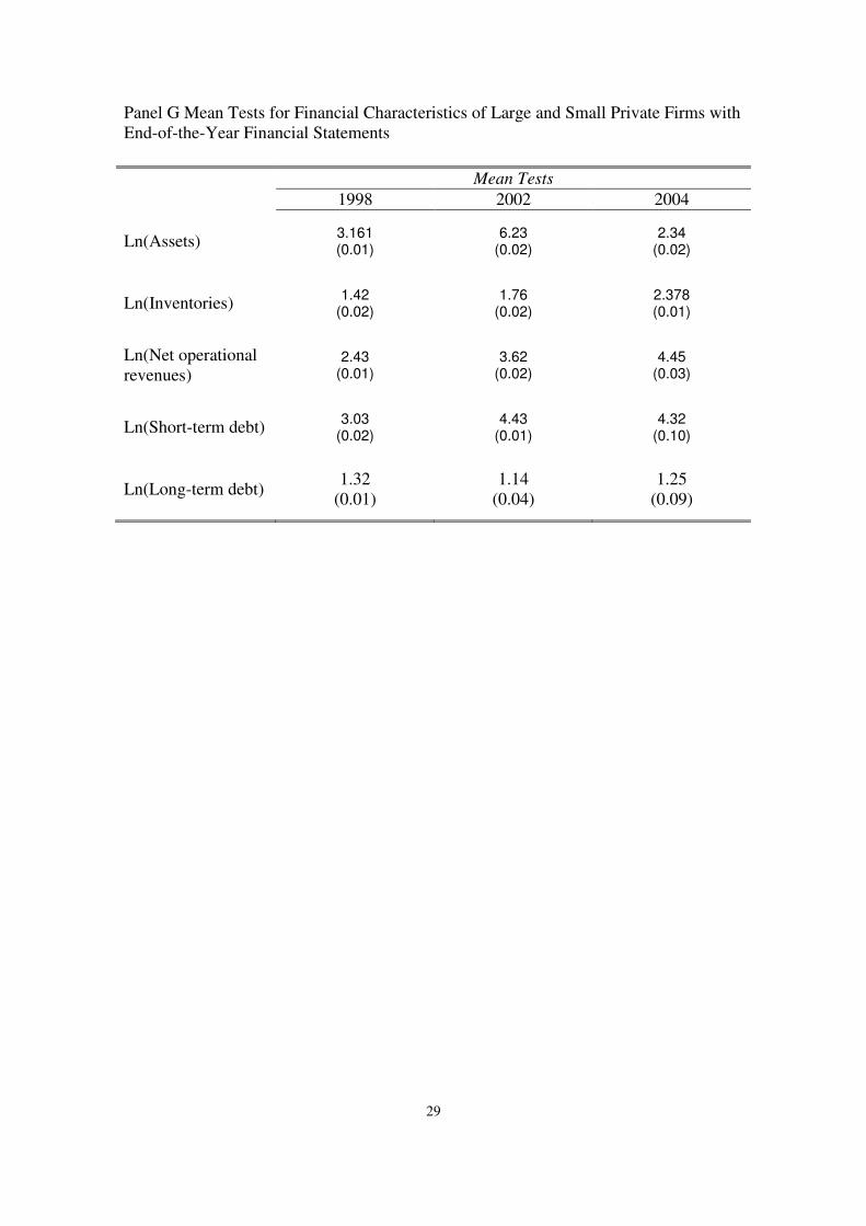
Panels F and G of Table 1 present the financial characteristics of small and large private

firms with end-of-the-year balance sheet information as well as their mean tests. Large

private firms have, on average, greater long-term and short-term debt than do small

private firms and more net operational revenues. Therefore, it seems that small private

firms in our sample differ as well from large firms as far as access to the financial

market is concerned. They seem to have also less access to the financial markets.

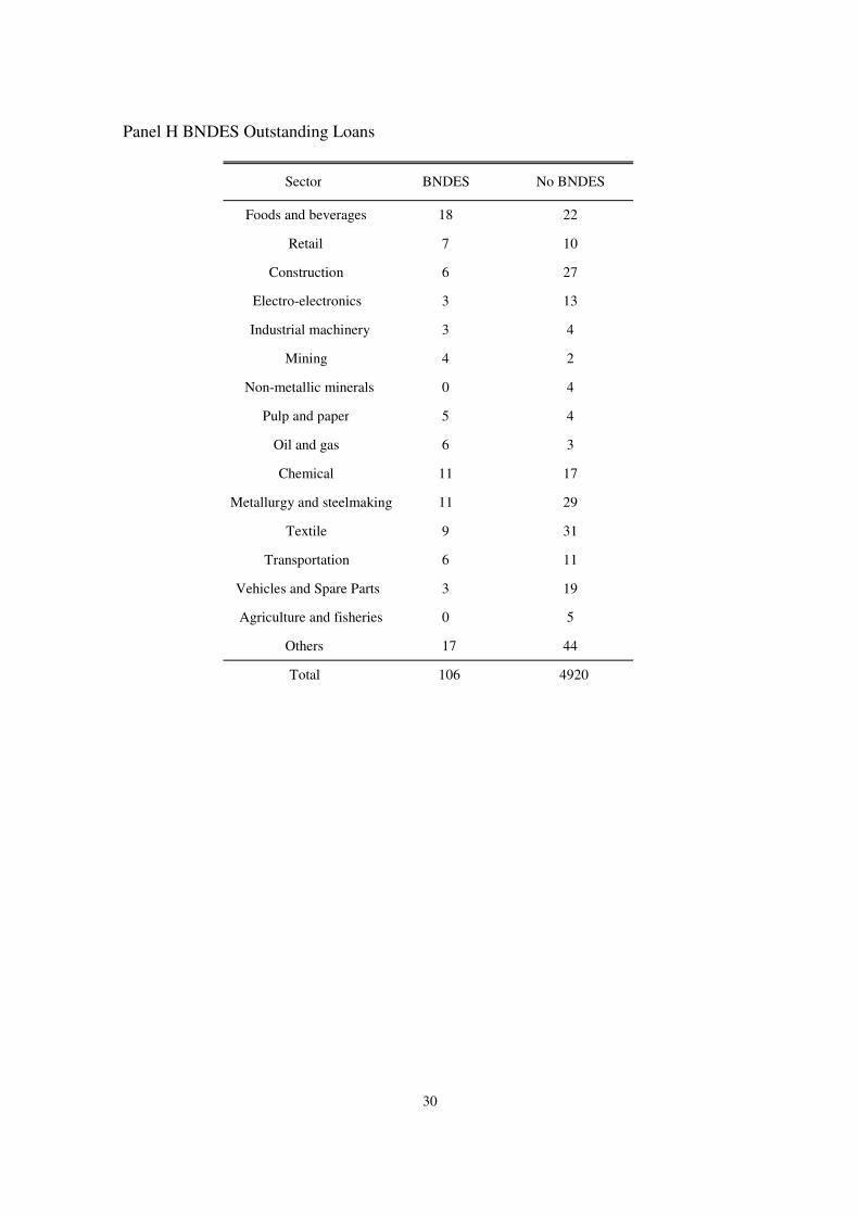
Finally, Panel H of Table 1 presents information about outstanding loans of firms in our

sample of firms with BNDES during our sample period. As one can see, there are 106

firms (21.09%) with outstanding loans. Most come from the food and beverages sector

(16.98%).13

In the next section, we will describe our model.

13

To obtain the information on BNDES we looked at off balance sheet information of public firms as

well as information disclosed on the homepage of BNDES at the Internet.

9

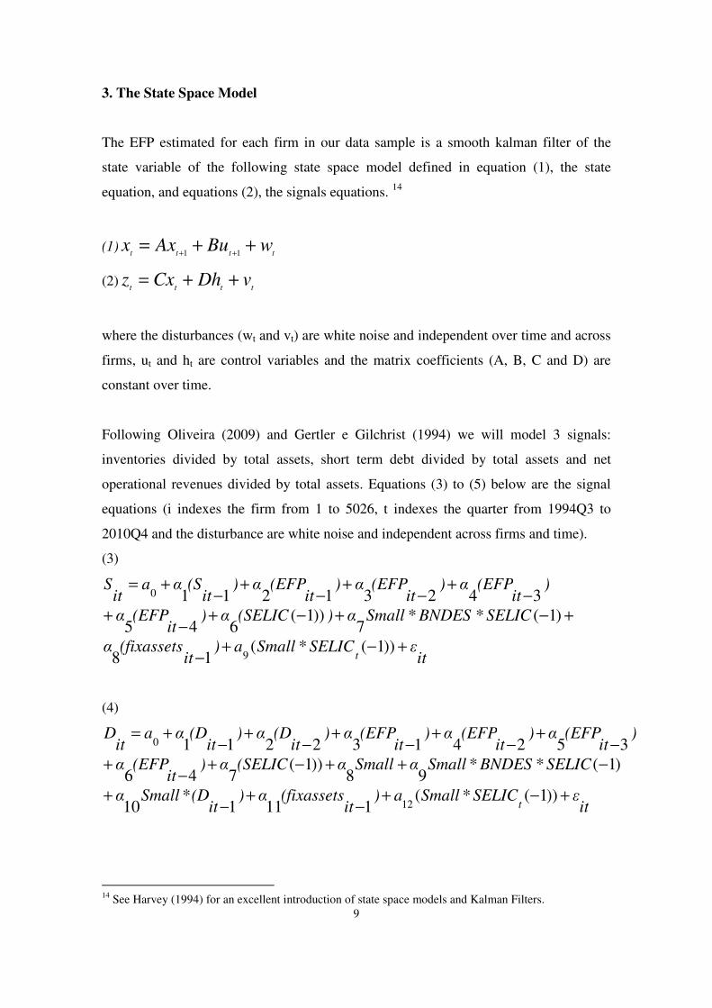
3. The State Space Model

The EFP estimated for each firm in our data sample is a smooth kalman filter of the

state variable of the following state space model defined in equation (1), the state

equation, and equations (2), the signals equations. 14

(1)tttt

wBuAxx ++=++ 11

(2)tttt

vDhCxz ++=

where the disturbances (wt and vt) are white noise and independent over time and across

firms, ut and ht are control variables and the matrix coefficients (A, B, C and D) are

constant over time.

Following Oliveira (2009) and Gertler e Gilchrist (1994) we will model 3 signals:

inventories divided by total assets, short term debt divided by total assets and net

operational revenues divided by total assets. Equations (3) to (5) below are the signal

equations (i indexes the firm from 1 to 5026, t indexes the quarter from 1994Q3 to

2010Q4 and the disturbance are white noise and independent across firms and time).

(3)

itεSELICSmalla)

it(fixassetsα

SELICBNDESSmallα)(SELICα)it

(EFPα

)it

(EFPα)it

(EFPα)it

(EFPα)it

(Sαait

S

t+−+

−

+−+−+−

+−

+−

+−

+−

+=

))1(*(18

)1(**7

))1(645

34231211

9

0

(4)

itεSELICSmalla)

it(fixassetsα)

it(DSmallα

SELICBNDESSmallαSmallα(SELICα)it

(EFPα

)it

(EFPα)it

(EFPα)it

(EFPα)it

(Dα)it

(Dαait

D

t+−+

−+

−+

−++−+−

+−

+−

+−

+−

+−

+=

))1(*(1111

*10

)1(**98

))1(746

3524132211

12

0

14

See Harvey (1994) for an excellent introduction of state space models and Kalman Filters.

10

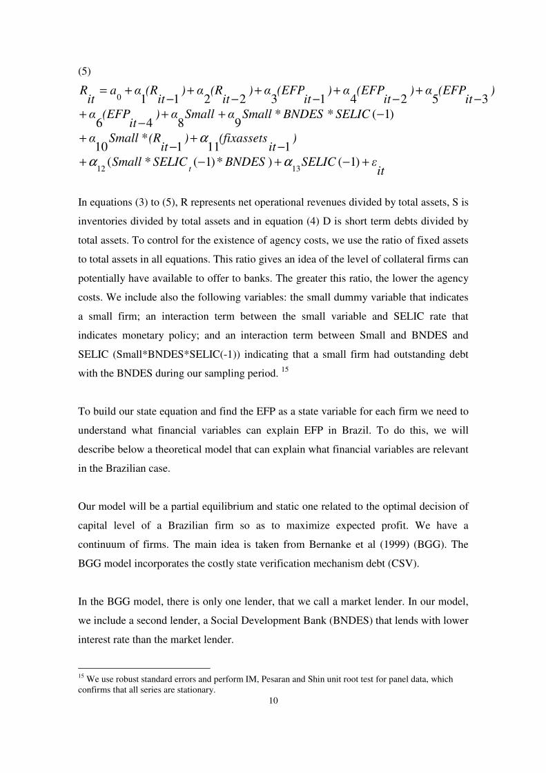
(5)

itεSELICBNDESSELICSmall

)it

(fixassets)it

(RSmallα

SELICBNDESSmallαSmallα)it

(EFPα

)it

(EFPα)it

(EFPα)it

(EFPα)it

(Rα)it

(Rαait

R

t+−+−+

−+

−+

−++−

+−

+−

+−

+−

+−

+=

)1()*)1(*(

1111*

10

)1(**9846

3524132211

1312

0

αα

α

In equations (3) to (5), R represents net operational revenues divided by total assets, S is

inventories divided by total assets and in equation (4) D is short term debts divided by

total assets. To control for the existence of agency costs, we use the ratio of fixed assets

to total assets in all equations. This ratio gives an idea of the level of collateral firms can

potentially have available to offer to banks. The greater this ratio, the lower the agency

costs. We include also the following variables: the small dummy variable that indicates

a small firm; an interaction term between the small variable and SELIC rate that

indicates monetary policy; and an interaction term between Small and BNDES and

SELIC (Small*BNDES*SELIC(-1)) indicating that a small firm had outstanding debt

with the BNDES during our sampling period. 15

To build our state equation and find the EFP as a state variable for each firm we need to

understand what financial variables can explain EFP in Brazil. To do this, we will

describe below a theoretical model that can explain what financial variables are relevant

in the Brazilian case.

Our model will be a partial equilibrium and static one related to the optimal decision of

capital level of a Brazilian firm so as to maximize expected profit. We have a

continuum of firms. The main idea is taken from Bernanke et al (1999) (BGG). The

BGG model incorporates the costly state verification mechanism debt (CSV).

In the BGG model, there is only one lender, that we call a market lender. In our model,

we include a second lender, a Social Development Bank (BNDES) that lends with lower

interest rate than the market lender.

15

We use robust standard errors and perform IM, Pesaran and Shin unit root test for panel data, which

confirms that all series are stationary.

11

The reason for this is a particular feature of Brazil’s credit market, as we stressed

before. In Brazil, BNDES is a key player in the implementation of government’s

industrial policy and the main long term financing provider for private investment. The

funds offered by BNDES have better costs and maturity conditions compared with other

financing agents from Brazil’s credit market. Furthermore, the long term interest rate

charged for funds obtained in the development bank16

are just marginally affected by

the short term interest rate that Central Bank controls. In such a context, firms that have

more access to BNDES funds must present more resilience to external finance premium

variation.17

We will assume that the probability a firm has to obtain a loan at BNDES is BP . To

apply for financing with BNDES resources, the client must meet the following

minimum requirements: be up to date with tax obligations; have ability to pay; have

sufficient guarantees against the risk of the operation; not be under a credit recovery

regime; and comply with legislation on the imports, in the case of financing for imports

of machinery and equipment; finally comply with environmental laws.

The firms are assumed to be risk neutral and have finite horizons. They acquire capital

K at a price Q at the end of period t for use in production in period t+1. At the end of

period t, the firm j has available net worth jtN 1+ and finances capital with internal funds

supplemented by external borrowing from a financial intermediary:

jtjttjt NKQB 1111 ++++ −= .

Ex-ante the expected revenue from investment project depends if the lender obtained a

loan at BNDES or at the market bank. It is given by tt

K

tB KQRw 1+ in the case of the

market bank and tt

K

tM KQRw 1+ in the case of BNDES as a lender, where BwMw , are

productivity disturbance for a firm that obtains a loan at the market lender and at

BNDES respectively. These disturbances are iid across firms and time.

16

TJLP – “Taxa de Juros de Longo Prazo” (Long Term Interest Rate). 17

In the homepage of BNDES, one can verify that the volume of loans as well as the number of firms

that have received loans has increased over time, particularly in recent years.

12

Adopting the CSV approach, an agency problem arises because intermediaries (market

Bank and BNDES) cannot observe BwMw , and need to pay an auditing cost if they

wish to observe the outcome. The financial contract is a standard debt contract including

the following bankruptcy clause: if _

MM ww > or BB ww_

> the firm pays off the loan in

full from revenues and keeps the residual. The lender receives tt

K

tB KQRw 1

_

+ in the case

of BNDES and tt

K

tM KQRw 1

_

+ in the case of a market bank.

If the firm defaults on its loan, the lender pays an auditing cost Bµ in the case of

BNDES and Mµ in the case of the market lender. BNDES receives what is found,

namely (1- )Bµ tt

K

tB KQRw 1

_

+ and the market bank receives (1- )Mµ tt

K

tM KQRw 1

_

+ . A

defaulting firm receives nothing.

It is reasonable to assume that the lender will issue the loan only if the expected gross

return to the firm equal´s the lenders relevant opportunity costs of lending. Because the

loan risk is perfectly diversifiable, the relevant opportunity cost of the lender is the

riskless rate Rt+1 (SELIC rate) in the case of the market lender and ρ Rt+1 ρ <1 in the

case of the BNDES.

Let FB(w) , and FM(w) be the probability of default in the case of a firm that obtained a

loan at BNDES and market bank respectively. Let

=

+

+

1

1

t

K

t

R

REs be the discounted return

on capital or the EFP.

The following propositions relate the EFP to the probability of default of firms and to

the probability a firm has to obtain a loan at BNDES.

13

Proposition 1

Considering the structure of the model defined above, the external finance premium,

EFP, is an increasing function of the probabilities of default of firms at BNDES and the

market lender.

Demonstration: See Appendix A

Proposition 2

Considering the structure of the model, defined above, the external finance premium,

EFP, is a decreasing function of the probability of the firm to obtain a loan at BNDES if

the expected profit of BNDES is less than the expected profit of the market lender.

Demonstration See Appendix A

Taking in consideration Propositions 1 and 2 above, EFP is related to the probability of

default of firms and to the probability of obtaining a loan at BNDES. The probability of

default is a function of agency costs that depend on leverage, the return on capital, the

price of capital and default costs.

We follow Smith and Stulz (1985) and take total debt divided by total assets as an

empirical approximation of the leverage ratio. We also use the ratio between current

assets and current liabilities. This variable shows the degree of the firm’s current

liquidity. Extremely liquid businesses will have less probability of bankruptcy.

Myers (1977) demonstrates that indebted businesses have distorted incentives in terms

of their policies for investment. To summarize, the distortion occurs due to the priority

that the creditors have over the shareholders for receiving cash flow generated by

corporations. Given this priority, the shareholders do not have incentives to contribute

resources for investments whose returns—because of the highly indebted situation—

will likely be used in the payment of debt. Excessive debt, however, can impede

lucrative projects from being implemented. Thus, creditors anticipate the conflict of

14

interest and incorporate their costs in the interest rate. We will use the SELIC rate ,

lagged one period so as to avoid problems of endogeneity, as an approximation for this

interest rate.

As Jensen and Meckling (1976) argue the higher the ratio between the fixed assets and

total assets, the greater the firm’s capacity to offer real collateral to creditors, that can

reduce the creditors’ loss due to financial stress and, consequently, reduce the incentives

to distort the investment policy. Therefore, a greater ratio between fixed assets and

total assets reduces the probability of default.

Rajan and Zingales (1995) show that a high ratio between a corporation’s market value

and the book value suggests that future gains (embedded in the market value of the

firm’s shares) still do not correspond to the value of the existing assets. Such a

corporation should have greater difficulty offering real collateral to creditors compatible

with the profitability of the existing investment opportunities. So we will use this ratio

as a control variable as well.

Another characteristic of a firm related to its cost of agency with creditors is its size.

Larger firms, in general, have greater reputation, a fact that can reduce costs of agency.

Therefore, we can expect that the size, defined by the total assets, reduce the probability

of the firm using hedge or speculation as explained by Rajan and Zingales (1995).

We also consider an explanatory variable that is related to both the costs of bankruptcy

and to the cost of agency with creditors: the firm’s profitability, as Rajan and Zingales

(1995) discuss. The firm’s profitability is defined as the ratio of the company’s net

revenue to its net worth. This variable gives an idea about the capacity of the

corporation to internally finance itself, avoiding the capital market or bank loans. The

less a company needs to finance externally, the less are the costs of bankruptcy.

We also follow Bernanke and Gertler (1995) and use the inverse of the coverage ratio as

a proxy for EFP.

15

To summarize, EFP in our model in time t will be a function of the following variables

also in time t with the exception of SELIC rate, that is lagged one period: fixed assets

divided by total assets; size, measured by a dummy variable equal to 1 if the firm is

small; profitability, measured by net revenues divided by net worth; inverse of coverage

ratio; market value divided by book value; current assets divided by current liabilities;

total debt divided by total assets and a binary variable that indicates that the firm

obtained an outstanding loan at BNDES in our sample period interacted with the

dummy small and the SELIC rate.

Equation (6) below shows the state equation (i indexes the firm from 1 to 5026, t

indexes the quarter from 1994Q3 to 2010Q4, L is the lag function and the disturbance is

white noise and independent across firms and time). 18

(6)

itεSELICSELICSmallacontrol

SELICBNDESSmallαSmallα)it

L(EFPait

EFP

it

tititi

+−+−+Π

+−++−

Γ+=

)1(*)))1(*(6

)1(**2110

5α

4- Empirical Analysis

One problem to estimate our state space model, equations (3) to (6), is that we have

much not available information of firms, particularly private firms with annual balance

sheet information only. So we backcast all control and signal series used in equations

(3) to (6).

There are many techniques to do this.19

We follow Issler et al (2009). In this case,

missing values will be the state variables described by the smooth kalman filter state

variable of the model below for each variable of interest and for each firm (i indexes the

firm from 1 to 5026 and t indexes the quarter from 1994Q3 to 2010Q4).

ititSI ∆=∆ for t=1994Q3 to 2010Q4

tI∆ missing

18

The number of lags for each firm is obtained by the Akaike identification criteria. 19

See Chon e Lin (1971), Harvey e Pierse (1984) and Silva and Cardoso (2001).

16

ititII ∆=∆ otherwise (3)

ititititXSS εα +Β+∆=∆

−1

where,

I∆ - series of interest used as control or signal in our state space from (3) to (6)

measured in growth rate;

X– control variables: growth rate of real GDP, growth rate of real industrial production

and growth rate of services GDP.

S∆ - state variable at t

- White noise

After backcasting our controls and signal series, we estimate our state space model,

equations (3) to (6) for each firm. The EFP is the smooth kalman filter of the state

equation(6).

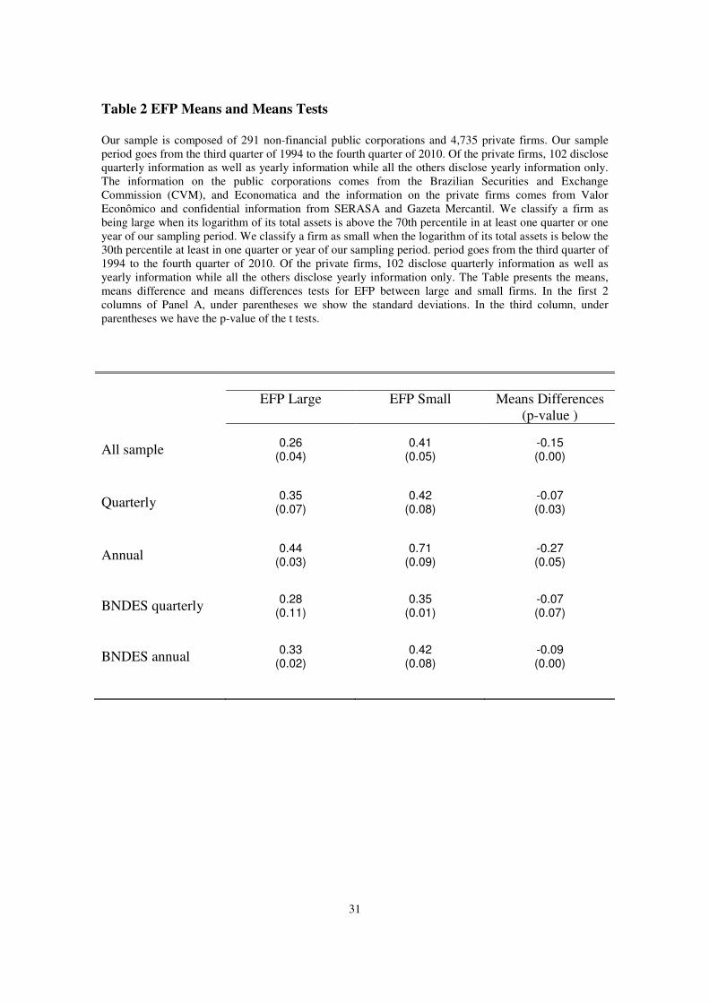
Table 2 presents the average of all EFP estimated for several classifications of firms.

One can observe that small firms in our sample have higher average and volatility of

EFP than large firms independently if they have quarterly or annual information or had

outstanding loans at BNDES during our sample period.

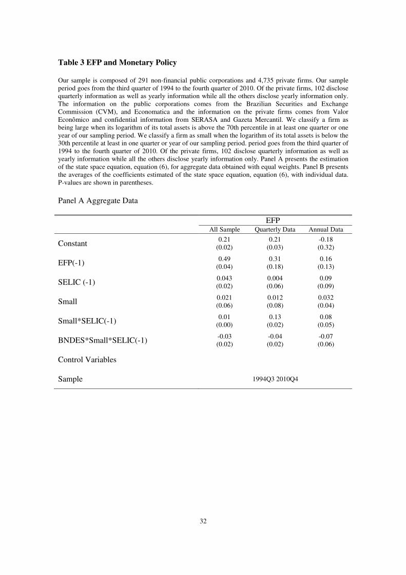
In Table 3 Panels A and B, we present the results of the estimation of the state equation

(6). We are interested in the sign of the following regressors: SELIC, the dummy

variable of the small firms alone and interacted with the SELIC rate and the interaction

between the Selic rate, the small variable and the BNDES dummy variable. If the

balance sheet explanation of the monetary policy is relevant, the coefficients of SELIC,

small and the interaction between the two are positive and significant. Due to the credit

market characteristics of the credit market in Brazil, we would expect also the

17

coefficient variable of the interaction between BNDES, small and SELIC to be negative

and significant.

Table 3 Panel A presents the results of the estimation of the state variable based on

aggregate data of all the series involved in our estimation for the whole sample, only for

firms that have quarterly information and for those firms with only annual information.

We aggregate the signal and control series using equal weights. As we can see all

coefficients have the right sign and are significant in all estimations for all types of

firms.

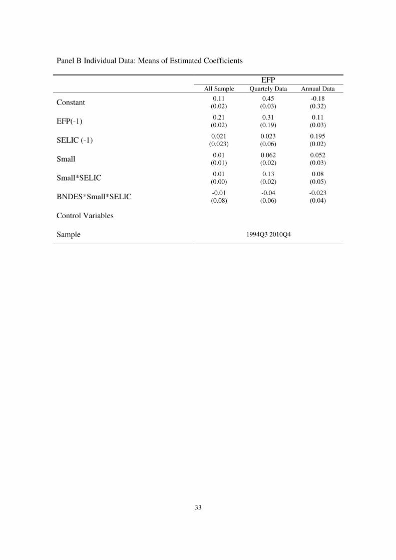
Table 3 Panel B presents the average of the coefficients of the estimation of the state

variables for each firm for the whole sample, only for firms that have quarterly

information and for those firms with only annual information.. As in Panel A, the

coefficients have the right sign and are statistically significant once more.

Panels A, B and C of Table 4 present the estimated coefficients of the signal equations,

that is the dynamics of inventories/assets, short-term debt/, and net operational

revenues/assets for aggregate data of all types of firms (equations (3) to (5)). We

aggregate the series of signal and controls using equal weights once more

For the dynamics of inventories /assets, short-term debt/assets, we are interested in the

sign of the following coefficients: the sum of the EFP coefficients; SELIC; the dummy

variable of the small firms alone and interacted with the SELIC rate; and the interaction

between the Selic rate, the small variable and the BNDES dummy variable. If the

balance sheet explanation of the monetary policy is consistent, the sum of EPP

coefficients, and the coefficients of SELIC, small and the interaction between the two

are positive and significant. Due to the credit market characteristics of the credit market

in Brazil, we would expect the coefficient variable between BNDES, small and SELIC

to be negative and significant. As one can observe, all coefficients have the right sign

and are significant.

For the dynamics of net operational revenues/assets, we are interested in the sign of the

following coefficients: the sum of EFP coefficients; the coefficients of SELIC;, the

18

dummy variable of the small firms alone and interacted with the SELIC rate and the

interaction between the Selic rate, the small variable and the BNDES dummy variable.

If the balance sheet explanation of the monetary policy is relevant prevalent, the sum of

EFP coefficients, the coefficients of SELIC, small and the interaction between the two

are negative and significant. Once more, due to the credit market characteristics of the

credit market in Brazil, we would expect the coefficient variable between BNDES,

small and SELIC to be positive and significant. As we can observe, all coefficients have

the right sign and are significant.

Panels A, B and C of Table 5 present the averages of the estimated coefficients of the

signal equations, that is the dynamics of inventories/assets, short-term debt/, and net

operational revenues/assets for the estimations with individual data of all types of

firms.20

The coefficients reported are averages of the coefficients of all firms (standard

deviation of the averages in parenthesis). As we can see, all coefficients have the correct

sign (as we discussed above) and are statistically significant.

The results for the dynamics of the three variables - inventories/assets, net operational

revenues/assets, and short-term debt/assets- using individual data seem to confirm the

results we obtained with aggregated data. They indicate that small and large public

firms react very differently to monetary policy. Small firms seem to be more sensitive to

monetary policy than large firms.

Maybe our previous results have some relation to the fact that we have more small firms

than large firms. To verify whether this is driving our results, we decreased the number

of small firms in all estimations presented above such that it would match the number of

large firms. Due to space restrictions, we do not report our results, but they confirm, in

general, the previous ones.

We also did several other robustness exercises. We used several different specifications

for the state and signal equations. We used the growth rate of BOVESPA and IBRX as

control variables in the backcasting estimations. We aggregated the data in Table 3 and

4 using weights proportional to the total assets of firms. We use medians instead of

19

averages for the coefficients estimated in Table 3 Panel B and Table 5 Panels A, B and

C. We included a control variable that indicates a financial crisis in Brazil in our

sampling period in the state and signal equations. In general, our results do not change.

Due once again to space restrictions, we do not report the results.

All our empirical results above seem to show a relevant asymmetry in the reaction of

small and large firms to monetary contractions. This asymmetry reflects different access

of Brazilian corporations to the financial markets. Large public and private firms have

more financing alternatives than do their small counterparts and therefore are able to

suffer less discontinuity in terms of investment, revenues and short-term financing after

monetary contractions.

Since the borrowers’ financial position affects their external premium and thus the

overall terms of credit they face, fluctuations in the quality of borrowers’ balance sheets

should likewise affect their investment and spending decisions.

This approach has been supported by a wide range of empirical work linking balance

sheet and cash flow variables to firms’ decisions concerning fixed investments,

inventories and other factor demands, as well as to household purchases of durables and

housing.

The balance sheet channel of monetary policy arises because shifts in the central bank

policy not only affect the market interest rate per se, but also the borrowers’ financial

positions both directly and indirectly. Our paper is in line with this overall empirical

evidence of the literature for OECD countries.

20

We use robust standard errors in our regressions to correct for autocorrelation and heteroskedasticity.

20

5. Conclusion

This paper investigates the balance sheet explanation of the monetary transmission

mechanism in Brazil. One problem to investigate this is that a fundamental variable for

this purpose, the external finance premium (EFP), is non observable. This paper

contributes to the literature by estimating the EFP of firms in Brazil using state space

models.

Our estimations are based on an original database with confidential and public data

containing information of 5,026 public and private firms from the third quarter of 1994

to the fourth quarter of 2010.

Our results show that the average and volatility of the EFP of small firms is higher than

those of large firms and that the EFP is more sensitive to monetary policy for small

firms than for large firms. We also found that the elasticity of EFP in relation to

inventories, short term debt and net operational revenues, all as a proportion of total

assets is higher for small firms than for large firms. These empirical evidences point to

the importance of the balance sheet channel as an explanation for the transmission

mechanism of monetary policy in Brazil.

Our results indicate that small firms are much more sensitive to monetary policy than

large firms and that BNDES plays a relevant role in decreasing this sensitiveness. The

results are robust to several different specifications of the space model.

Large firms in Brazil which are likely to obtain loans from the BNDES as well as

external finance typically respond to an unanticipated decline in cash flows in a

different manner from small firms. They can at least temporally be able to maintain

their levels of production and employment in the face of higher interest costs and

declining revenues through other sources of short-term and long-term financing.

However, this is not the case for small firms. These firms, which have more limited

access to the financial markets, tend to lose inventories and revenues and to cut work

hours and production.

21

These differences in access have many possible reasons. Some have to do with a

bankruptcy legislation that makes it difficult for creditors to size the assets of firms;

others relate to high spreads that are still prevalent in Brazil; another reason as well may

be related to a segmented credit market, where long-term financing basically comes

from the BNDES and is much easier for large firms, which meet the necessary

requisites for the loans, than for small firms.

REFERENCES

Bernanke, Ben.S, and Gertler, Mark., “Inside the Black Box: The Credit Channel of

Monetary Policy Transmission Mechanism,” Journal of economic Perspectives 9, 27-48

Bernanke, B., Gertler, M. and Gilchrist, S.: 1999, The financial accelerator in a

quantitative business cycle framework, in J. Taylor and M. Woodford (eds), Handbook

of Macroeconomics, Vol. 1C, Elsevier Science, North Holland.

Caballero, R.J. and Krishnamurth, A.. "International Domestic Collateral Constraints in

a Model of Emerging Market Crises." Journal of Monetary Economics, 48 (2001), 513-

548

Chow, C. Gregory e Lin, An-IOh. Best Linear Unbiased Interpolation, Distribution and

Extrapolation of Time Series by Related Series. The Review of Economic and Statistics,

vol 53, No 4 (1971(, 372-375

Gertler, M. and Lown, C.: 1999, The information in the high-yield bond spread for the

business cycle: Evidence and some implications, Oxford Review of Economic Policy

15, 132–150.

Gertler, Mark and Gilchrist Simon “Monetary Policy, Business Cycles and the

Behaviour of Small Manufacturing Firms.” The Quarterly Journal of Economics, Vol

109, No. 2 (May, 1994), 309-340

22

Gilchrist, Simon; Himmelberg, Charles P. (1995). “Evidence on the Role of Cash Flow

for Investment” In: Journal of Monetary Economics, n. 36, p. 541-572.

Gilchrist, Simon; Hilmlberg, Charles P. (1998). “Investment, Fundamentals, and

Finance” In: National Bureau of Economic Research. NBER Working paper series

6652.

Harvey, C. Andrew. Time Series Analysis MIT Press 1994

Issler, J.V., Notini, H.H. e Rodrigues, F.C. Um Indicador Coincidente e Antecedente da

Atividade Econômica Brasileira. Ensaios Econômicos FGV Fevereiro de 2009.

Kashyap, Stein, and Wilcox (1993). Monetary Policy and Credit Conditions: Evidence

from the Composition of External Finance.” The American Economic Review, pp. 78-

98.

Jensen, C. Michael and Meckling, H. William. "Theory of the Firm: Managerial

Behavior, Agency Costs and Ownership Structure". Journal of Financial Economics, 3,

1976, 305-360

Levin, A., Natalucci, F. and Zakrajsek, E.: 2004, The magnitude and cyclical behaviour

of financial market frictions’, Working Paper 2004–70, Board of Governors of the

Federal Reserve System.

Graeve, Ferre D. (2008). “The External Finance Premium and the Macroeconomy: US

post-WWII Evidence.”In: Federal Reserve Bank of Dallas, Working Paper nº 0809.

Mishkin, Frederick S. The Transmission Mechanism and the Role of Asset Prices in

Monetary Policy. NBER 8617, December 2001

----------------- The Channels of Monetary Transmission: Lessons for Monetary Policy.

NBER 5464, February 1996

----------------- "Financial Policies and the Prevention of Financial Crises in Emerging

Market Countries." NBER 8087, January 2001.

23

Mody, A. and Taylor, M.: 2004, Financial predictors of real activity and the financial

accelerator, Economics Letters 82, 167–172.

Myers, S. “Determinants of Corporate Borrowing”, Journal of Financial Economics, 3,

1977, 147 – 175.

Oliveira, Fernando N. (2009). “Effects of Monetary Policy on Corporations in Brazil:

An Empirical Analysis of the Balance Sheet Channel”. Brazilian Review of

Econometrics 29, Number 2 November 2009.

Rajan, Raghuram G & Zingales, Luigi, “What Do We Know about Capital Structure?

Some Evidence from International Data," Journal of Finance, American Finance

Association, vol. 50(5), pages 1421-60, December 1995.

Silva, S.M.J e Cardoso,F.N.. The Chow-Lin Model Using Dynamic Models. Economic

Modelling 18(2001) 269-280.

Smith, W. Clifford and Stulz, M. René. "The Determinants of Firms Hedging Policies".

Journal of Financial and Quantitative Analysis, 20, 1985, 391-405.

24

Table 1. Descriptive Analysis of the Database

Our sample is composed of 291 non-financial public corporations and 4,735 private firms. Our sample

period goes from the third quarter of 1994 to the fourth quarter of 2010. Of the private firms, 102 disclose

quarterly information as well as yearly information while all the others disclose yearly information only.

The information on the public corporations comes from the Brazilian Securities and Exchange

Commission (CVM), and Economatica and the information on the private firms comes from Valor

Econômico and confidential information from SERASA and Gazeta Mercantil. We classify a firm as

being large when its logarithm of its total assets is above the 70th percentile in at least one quarter or one

year of our sampling period. We classify a firm as small when the logarithm of its total assets is below the

30th percentile at least in one quarter or year of our sampling period. Panel A shows the number of

private and public firms separated by sectors of the economy. Panel B shows small and large private and

public firms with quarterly information organized by sectors of the economy. Panel C shows some

financial characteristics of small and large firms with quarterly financial statements. Panel D shows the

results of the mean tests for the financial characteristics of small and large firms with quarterly financial

statements. Panel E shows small and large private firms with end-of-the-year information organized by

sectors of the economy. Panel F shows some financial characteristics of small and large private firms with

end-of-the-year financial statements. Panel G shows the results of the mean tests for the financial

characteristics of small and large private firms with end-of-the-year financial statements. Panel H shows

the number of private and public firms that had loans with BNDES during our sample period.

Panel A Total Number of Firms Classified by type (private or public) and sectors

Public Private

Chemical/Petroleum 36 273

Foods and Beverage 40 90

Mining/Metalurgy 8 31

Eletrical/Eletronic 14 92

Transportation 18 268

Public Services 30 91

Textile 35 75

Services 39 1110

Others 71 3815

Total 291 4,735

25

Panel B Small and Large Firms with Quarterly information by Sectors of the Economy

Sectors

Large Small T

o

t

a

N Log(Assets) Net Operational

Revenues/Assets N Log(Assets) Net Operational Revenues/Assets

Chemical/Petroleum 4 19.21 0.69 1 18.36 0.45 1

5

Food and Beverages 11 18.24 0.51 10 17.56 0.34 2

4

Mining/Metallurgy 4 18.31 0.44 8 17.90 0.71 2

6

Electro/Electronic

Equipment 3 18.61 0.58

8

17.81

0.45

3

2

Transportation 5 18.49 0.41 6 17.86 0.51 2

0

Public Services

16 18.39 0.71 6 17.51 0.73 4

6

Textiles 4 18.67 0.55 13 16.21 0.54 2

9

Services 3 11.80 0.31 14 9.72 0.49 3

5

Others 18 10.32 0.72 54 10.45 0.31

1

6

6

Private Firms 5 11.41 0.38 39 8.32 0.56

1

0

2

Total 68 120

3

9

3

Panel C Financial Characteristics of Firms with Quarterly Information

Financial

Characteristics

Large Firms

(A)

Small Firms

(B)

N Mean Median Standard

Deviation N Mean Median Standard Deviation

Log(Assets) 68 18.31 18.05 4.19 120 17.17 17.05 3.51

Operational

revenues/Assets 68 0.68 0.60 0.85 120 0.36 0.18 0.58

Financial

Expenses/Assets 68 0.19 0.18 0.35 120 0.19 0.19 0.42

Fixed Assets/

Assets 68 0.47 0.53 0.46 120 0.36 0.36 0.83

26

Short-term

Debt/Assets) 68 0.68 0.65 0.91 120 0.49 0.17 0.15

Long-term

Debt/Assets 68 0.23 0.19 0.17 120 0.09 0.12 0.13

BNDES Loans

36

21

Panel D Mean Tests for Financial Characteristics of Large and Small Firms with

Quarterly Information

Mean Tests

4Q1994 4Q2002 4Q2010

Ln(Assets) 4.33

(0.03) 4.96

(0.03) 5.70

(0.03)

Ln (inventories) 2.55

(0.06) 3.66

(0.01) 2.95

(0.02)

Ln(net operational

revenues) 3.44

(0.01) 3.06

(0.01) 4.52

(0.02)

Ln(short-term debt) 3.470 (0.00)

3.09 (0.02)

4.87 (0.01)

Ln(long-term debt) 1.82

(0.01)

1.99

(0.01)

1.58

(0.02)

Panel E Small and Large Private Firms with End-of-the-Year Information and Sectors

of the Economy

Sectors

Large Small T

o

t

a

N Log(Assets) Net Operational

Revenues/Assets N Log(Assets) Net Operational Revenues/Assets

Chemical/Petroleum 10 12.18 0.61 8 9.26 0.59

1

1

5

Food and Beverages 20 9.26 0.43 10 10.46 0.36

1

3

9

27

Mining/Metallurgy 10 11.25 0.23 16 10.24 0.27

1

2

9

Electro/Electronic

Equipment 7 10.17 0.53 12

11.14

0.18

3

4

Transportation 9 9.20 0.56 21 8.75 0.24

1

0

1

Public Services

14 8.30 0.49 5 7.29 0.40 4

2

Textiles 13 8.21 0.16 14 9.27 0.78

1

4

5

Services 6 19.54 0.24 49 11.30 0.64

1

0

4

Others 13.23 0.38 7.09 0.45

3

,

9

8

8

Total 108 181

4

,

7

9

7

28

Panel F Financial Characteristics of Private Firms with End-of-the-Year Information

Financial

Characteristics

Large Firms

(A)

Small Firms

(B)

N Mean Median Standard

Deviation N Mean Median Standard Deviation

Log(Assets) 108 11.87 11.0 3.51 181 8.32 8.70 4.76

Net Operational

revenues/Assets 108 0.61 0.42 2.65 181 0.31 0.47 0.49

Financial

Expenses/Assets 108 0.15 0.05 1.28 181 0.19 0.16 0.29

Fixed Assets/

Assets 108 0.63 0.35 0.43 181 0.47 0.31 0.61

Short-term

Debt/Assets) 108 0.41 0.41 0.61 181 0.39 0.14 0.51

Long-term

Debt/Assets 108 0.32 0.05 0.31 181 0.28 0.23 0.29

29

Panel G Mean Tests for Financial Characteristics of Large and Small Private Firms with

End-of-the-Year Financial Statements

Mean Tests

1998 2002 2004

Ln(Assets) 3.161 (0.01)

6.23 (0.02)

2.34 (0.02)

Ln(Inventories) 1.42

(0.02) 1.76

(0.02) 2.378 (0.01)

Ln(Net operational

revenues) 2.43

(0.01) 3.62

(0.02) 4.45

(0.03)

Ln(Short-term debt) 3.03

(0.02) 4.43

(0.01) 4.32

(0.10)

Ln(Long-term debt) 1.32

(0.01)

1.14

(0.04)

1.25

(0.09)

30

Panel H BNDES Outstanding Loans

BNDES No BNDESSector

Retail

Non-metallic minerals

27 Construction 6

4

4

7 10

Foods and beverages 18 22

Industrial machinery 3

Electro-electronics 3 13

0

3

Mining 4 2

Oil and gas 6

Textile 9 31

29

Pulp and paper 5 4

Metallurgy and steelmaking 11

Vehicles and Spare Parts 3

11

Chemical 11 17

Transportation 6

Total 106 4920

Agriculture and fisheries 0

19

5

44 17 Others

31

Table 2 EFP Means and Means Tests









30th percentile at least in one quarter or year of our sampling period. period goes from the third quarter of

1994 to the fourth quarter of 2010. Of the private firms, 102 disclose quarterly information as well as

yearly information while all the others disclose yearly information only. The Table presents the means,

means difference and means differences tests for EFP between large and small firms. In the first 2

columns of Panel A, under parentheses we show the standard deviations. In the third column, under

parentheses we have the p-value of the t tests.

EFP Large EFP Small Means Differences

(p-value )

All sample 0.26

(0.04) 0.41

(0.05) -0.15 (0.00)

Quarterly 0.35

(0.07) 0.42

(0.08)

-0.07 (0.03)

Annual 0.44

(0.03) 0.71

(0.09) -0.27 (0.05)

BNDES quarterly 0.28

(0.11) 0.35

(0.01) -0.07 (0.07)

BNDES annual 0.33

(0.02) 0.42

(0.08) -0.09 (0.00)

32

Table 3 EFP and Monetary Policy











yearly information while all the others disclose yearly information only. Panel A presents the estimation

of the state space equation, equation (6), for aggregate data obtained with equal weights. Panel B presents

the averages of the coefficients estimated of the state space equation, equation (6), with individual data.

P-values are shown in parentheses.

Panel A Aggregate Data

EFP All Sample Quarterly Data Annual Data

Constant 0.21

(0.02)

0.21

(0.03)

-0.18

(0.32)

EFP(-1) 0.49

(0.04)

0.31

(0.18)

0.16

(0.13)

SELIC (-1) 0.043

(0.02)

0.004

(0.06)

0.09

(0.09)

Small 0.021

(0.06)

0.012

(0.08)

0.032

(0.04)

Small*SELIC(-1) 0.01

(0.00)

0.13

(0.02)

0.08

(0.05)

BNDES*Small*SELIC(-1) -0.03

(0.02)

-0.04

(0.02)

-0.07

(0.06)

Control Variables

Sample 1994Q3 2010Q4

33

Panel B Individual Data: Means of Estimated Coefficients

EFP All Sample Quartely Data Annual Data

Constant 0.11

(0.02)

0.45

(0.03)

-0.18

(0.32)

EFP(-1) 0.21

(0.02)

0.31

(0.19)

0.11

(0.03)

SELIC (-1) 0.021

(0.023)

0.023

(0.06)

0.195

(0.02)

Small 0.01

(0.01)

0.062

(0.02)

0.052

(0.03)

Small*SELIC 0.01

(0.00)

0.13

(0.02)

0.08

(0.05)

BNDES*Small*SELIC -0.01

(0.08)

-0.04

(0.06)

-0.023

(0.04)

Control Variables

Sample 1994Q3 2010Q4

34

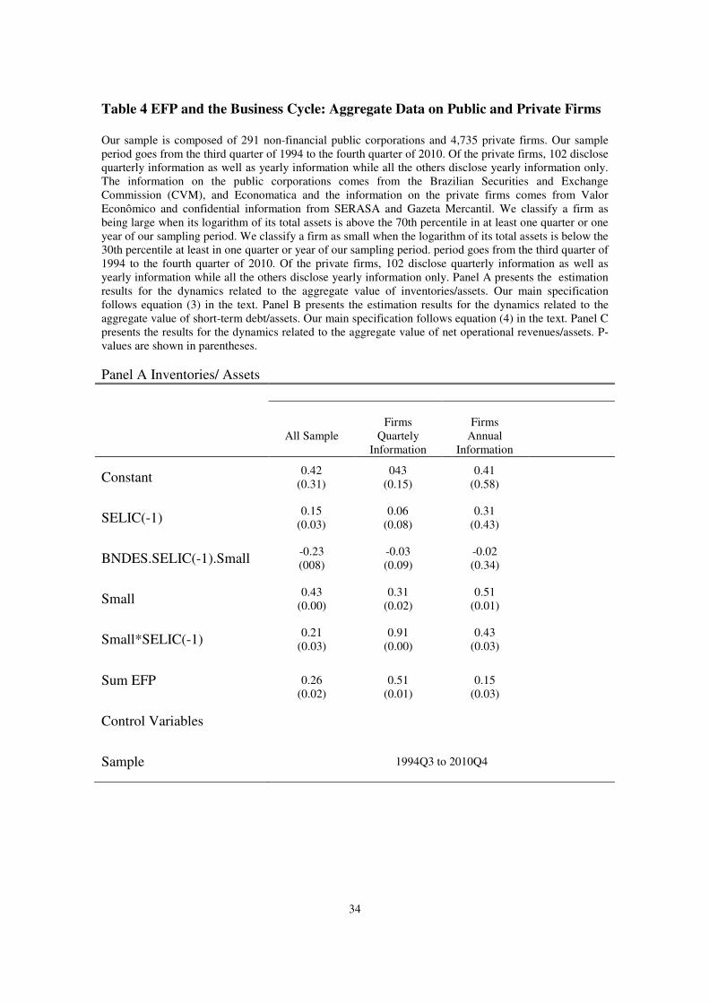
Table 4 EFP and the Business Cycle: Aggregate Data on Public and Private Firms











yearly information while all the others disclose yearly information only. Panel A presents the estimation

results for the dynamics related to the aggregate value of inventories/assets. Our main specification

follows equation (3) in the text. Panel B presents the estimation results for the dynamics related to the

aggregate value of short-term debt/assets. Our main specification follows equation (4) in the text. Panel C

presents the results for the dynamics related to the aggregate value of net operational revenues/assets. P-

values are shown in parentheses.

Panel A Inventories/ Assets

All Sample

Firms

Quartely

Information

Firms

Annual

Information

Constant 0.42

(0.31)

043

(0.15)

0.41

(0.58)

SELIC(-1) 0.15

(0.03)

0.06

(0.08)

0.31

(0.43)

BNDES.SELIC(-1).Small -0.23

(008)

-0.03

(0.09)

-0.02

(0.34)

Small 0.43

(0.00)

0.31

(0.02)

0.51

(0.01)

Small*SELIC(-1) 0.21

(0.03)

0.91

(0.00)

0.43

(0.03)

Sum EFP

0.26

(0.02)

0.51

(0.01)

0.15

(0.03)

Control Variables

Sample 1994Q3 to 2010Q4

35

Panel B Short-Term Debt/Assets

All Sample

Firms

Quartely

Information

Firms

Annual

Information

Constant -0.18

(0.33)

-0.69

(0.28)

-0.40

(0.23)

SELIC(-1) 0.15

(0.03)

0.06

(0.08)

0.31

(0.43)

Small 0.82

(0.03)

0.42

(0.01)

0.52

(0.04)

Small.SELIC(-1) 0.72

(0.00)

0.53

(0.03)

0.41

(0.01)

BNDES.SELIC(-1).Small -0.51

(0.08)

-0.42

(0.02)

-0.43

(0.04)

Sum EFP 0.16

(0.00)

0.311

(0.03)

0.18

(0.09)

Control Variables


Panel C Net Operational Revenues/ Assets

All sample

Firms

Quartely

Information

Firms

Annual

Information

Constant -0.71

(0.21)

-0.81

(0.29)

-0.21

(0.69)

SELIC(-1) -0.15

(0.03)

-0.06

(0.08)

0.31

(0.43)

Small -0.43

(0.03)

-0.61

(0.05)

-0.93

(0.08)

SELIC(-1).Small -0.52

(0.03)

-0.85

(0.01)

-0.76

(0.00)

BNDES.SELIC*Small(-1) 0.27

(0.08)

0.51

(0.01)

0.62

(0.04)

36

Sum EFP -0.22

(0.04)

-0.50

(0.06)

-0.19

(0.09)

Control Variables


37

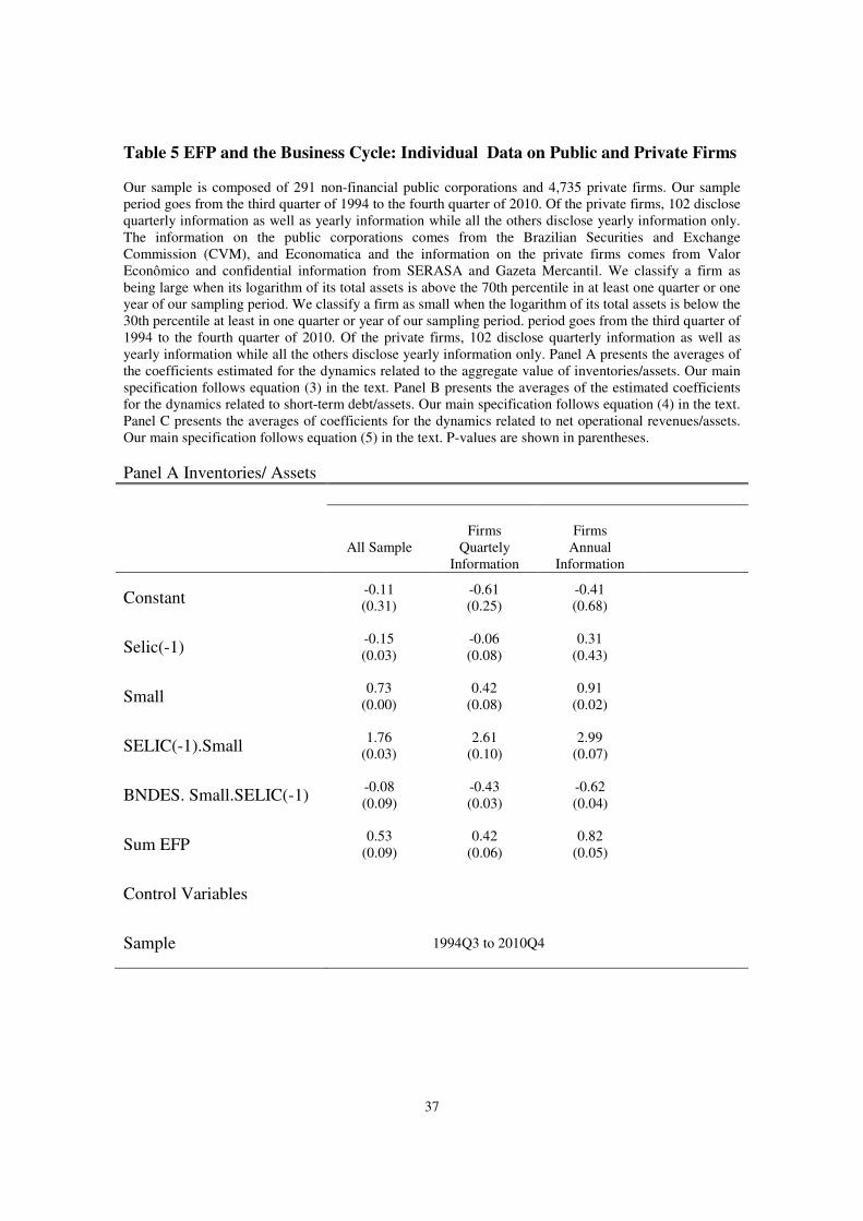
Table 5 EFP and the Business Cycle: Individual Data on Public and Private Firms











yearly information while all the others disclose yearly information only. Panel A presents the averages of

the coefficients estimated for the dynamics related to the aggregate value of inventories/assets. Our main

specification follows equation (3) in the text. Panel B presents the averages of the estimated coefficients

for the dynamics related to short-term debt/assets. Our main specification follows equation (4) in the text.

Panel C presents the averages of coefficients for the dynamics related to net operational revenues/assets.

Our main specification follows equation (5) in the text. P-values are shown in parentheses.

Panel A Inventories/ Assets

All Sample

Firms

Quartely

Information

Firms

Annual

Information

Constant -0.11

(0.31)

-0.61

(0.25)

-0.41

(0.68)

Selic(-1) -0.15

(0.03)

-0.06

(0.08)

0.31

(0.43)

Small 0.73

(0.00)

0.42

(0.08)

0.91

(0.02)

SELIC(-1).Small 1.76

(0.03)

2.61

(0.10)

2.99

(0.07)

BNDES. Small.SELIC(-1) -0.08

(0.09)

-0.43

(0.03)

-0.62

(0.04)

Sum EFP 0.53

(0.09)

0.42

(0.06)

0.82

(0.05)

Control Variables


38

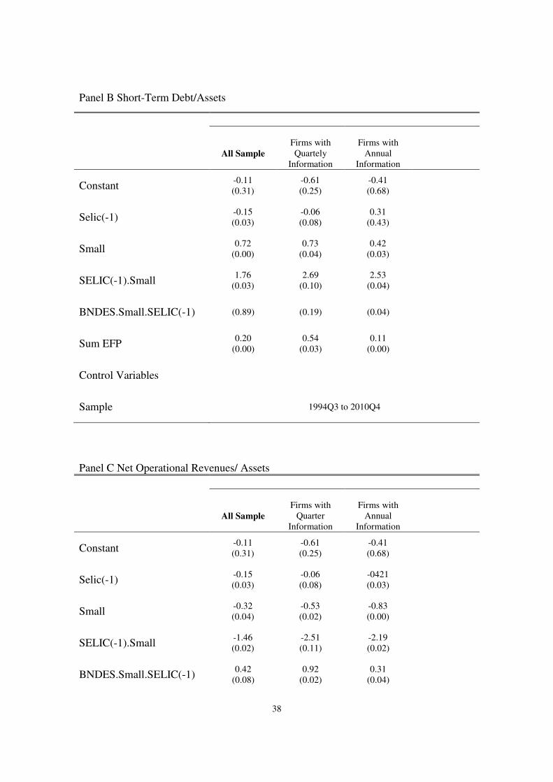
Panel B Short-Term Debt/Assets

All Sample

Firms with

Quartely

Information

Firms with

Annual

Information

Constant -0.11

(0.31)

-0.61

(0.25)

-0.41

(0.68)

Selic(-1) -0.15

(0.03)

-0.06

(0.08)

0.31

(0.43)

Small 0.72

(0.00)

0.73

(0.04)

0.42

(0.03)

SELIC(-1).Small 1.76

(0.03)

2.69

(0.10)

2.53

(0.04)

BNDES.Small.SELIC(-1) (0.89) (0.19) (0.04)

Sum EFP 0.20

(0.00)

0.54

(0.03)

0.11

(0.00)

Control Variables


Panel C Net Operational Revenues/ Assets

All Sample

Firms with

Quarter

Information

Firms with

Annual

Information

Constant -0.11

(0.31)

-0.61

(0.25)

-0.41

(0.68)

Selic(-1) -0.15

(0.03)

-0.06

(0.08)

-0421

(0.03)

Small -0.32

(0.04)

-0.53

(0.02)

-0.83

(0.00)

SELIC(-1).Small -1.46

(0.02)

-2.51

(0.11)

-2.19

(0.02)

BNDES.Small.SELIC(-1) 0.42

(0.08)

0.92

(0.02)

0.31

(0.04)

39

Sum EFP -0.16

(0.03)

-043

(0.01)

-0.35

(0.15)

Control Variables


40

Appendix A

In this appendix, we demonstrate Propositions 1 and 2 in the text. Our model adapts the

part of the BGG (1999) model related to the decision of the entrepreneur to the

Brazilian credit market. The idea is to model this decision using the costly state

verification mechanism (CSV).

It is a static partial equilibrium model related to the decision of the firm to maximize

expected profit. We have a continuum of firms and two types of lender, a market lender

and another lender, a social development Bank (BNDES). There is no aggregate risk.

The following are definitions of variables we use.

Definitions

=BP Probability Loan BNDES

=Bw productivity shock of BNDES loan

=Mw productivity shock of market loan

=Bw_

default cutoff BNDES

=Mw_

default cutoff market

=)(wBf density probability default of loan obtained at BNDES

=)(wMf density probability default of loan obtained at market bank

=)(wBµ monitoring costs BNDES

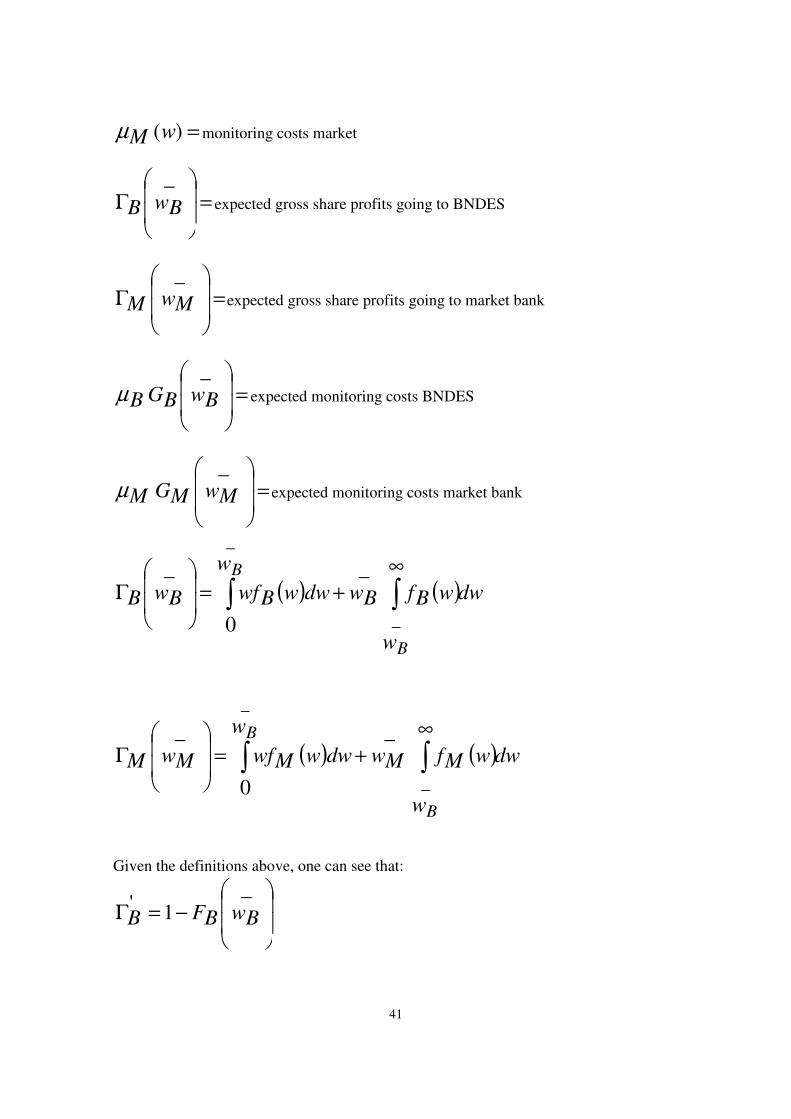
41

=)(wMµ monitoring costs market

=

Γ

_

BwB expected gross share profits going to BNDES

=

Γ

_

MwM expected gross share profits going to market bank

=

_

BwBGBµ expected monitoring costs BNDES

=

_

MwMGMµ expected monitoring costs market bank

( ) ( )dw

w

wBfBwdww

w

BwfBwB

B

B

∫∫∞

+=

Γ

_

_

_

0

_

( ) ( )dw

w

wMfMwdww

w

MwfMwM

B

B

∫∫∞

+=

Γ

_

_

_

0

_

Given the definitions above, one can see that:

−=Γ

_1'

BwBFB

42

−=Γ

_''

BwBfB

−=Γ

_1'

BwBFM

−=Γ

_1'

BwBFM

∫=

_

0

)(_ Bw

dwwBwfBBwBGB µµ

∫=

_

0

)(_ Bw

dwwBwfBBwBGB µµ

The Net Share Profit for BNDES and the market bank are:

BNDES: 0__

>

−

Γ BwBGBBwB µ

Market Bank: 0__

>

−

Γ MwMGMMwM µ

We have the following transversality conditions:

43

0__

lim

0_

=

−

Γ

→

BwBGBBwB

Bw

µ

0__

lim

0_

=

−

Γ

→

MwMGMMwM

Bw

µ

BBwBGBBwB

Bw

µµ −=

−

Γ

∞→

1__

lim_

MMwMGMMwM

Bw

µµ −=

−

Γ

∞→

1__

lim_

The hazards rate for the BNDES and Market bank loans are the following:

Hazard rate for BNDES=

−

_1

_

BwBF

BwBf

Hazard rate for Market Bank=

−

_1

_

MwMF

MwMf

44

As one can see,

__

BwhBw is increasing in

_

Bw

__

MwhMw is increasing in

_

Mw

There are global maximum for the net profits of firms that obtain a loan at BNDES and

at the market bank.

−

−=

−

Γ

__1

_1(

_'

_'

BwhBwBBwFBwBGBBwB µµ >=<

for *

_

BwBw >

−

−=

−

Γ

__1

_1(

_'

_'

MwhMwMMwFMwMGMMwM µµ

>=< for *

_

MwMw >

Proposition 1

Given the structure of the model described above an in the text, the external finance

premium, EFP, is an increasing function of the probabilities of default of firms.

Demonstration

A firm has the following problem to solve and it chooses: K, Bw

_Mw

_

45

( ) QKR KMMBBBB wPwPMax

Γ−−+

Γ−

__

111

s.t.

( )NQKRQKK

RBwBGBBwB −=

−

Γ ρµ

__

( )NQKRQKK

RMwMGMMwM −=

−

Γ

__µ

We define

10,, <<== ρN

QKk

R

KR

s

Where s is the external finance premium, EFP. Therefore, we will have:

46

( ) skMMBBBB wPwPMax

Γ−−+

Γ−

__

111

s.t.

1__

−=

−

Γ kk

sBwBGBBwB

ρµ

1__

−=

−

Γ kskMwMGMMwM µ

Or

( ) skMMBBBB wPwPMax

Γ−−+

Γ−

__

111

s.t.

022____

=+−

−

Γ+

−

Γ kskMwMGMMwMk

sBwBGBBwB µ

ρµ

47

Solution

( ) +

Γ−−+

Γ−= skMMBBBB wPwPL

__

111

022____

=+−

−

Γ+

−

Γ λλµλ

ρµλ kskMwMGMMwMk

sBwBGBBwB

FOC

(i) ⇒=∂

∂0

k

L

( ) +

Γ−−+

Γ− sMMBBBB wPwP

__

111

02____

=−

−

Γ+

−

Γ λµλµ

ρ

λMwMGMMwMsBwBGBBwB

s

(ii) ⇒=

∂

∂0

_

Bw

L

0_

'_

'_

' =

−

Γ+

Γ− BwBG

BBwBks

BwBBskP µρ

λ

(iii) ⇒=

∂

∂0

_

Mw

L

48

0_

'_

'_

')1( =

−

Γ+

Γ−− MwMG

MMwMskMwMBPsk µλ

Combining (ii) and (iii), we have:

( )

−

Γ+

−

Γ

Γ−+

Γ

=_

'_

'_

'_

'1

_1

_'

MwMGMMwMBwBGBBwB

MwMBPBwBBP

µµρ

λ

0,,,,,

__>

= MBMBB wwP µµρλλ

( )

−

Γ

Γ−+

Γ

−

−

Γ+

−

Γ

Γ

−

Γ+

−

Γ

=

∂

∂

_"

_''1

_'1

_'

_'

_'

_'

_'1

_''

2_

'_

'_

'_

'1

1

_

BwBGBBwBMwMBPBwBP

MwMGMMwMBwBGBBwBBwBP

x

MwMGMMwMBwBGBBwBBw

µρ

µµρ

µµρ

λ

It is easy to see that 0_

<

∂

∂

Bw

λ

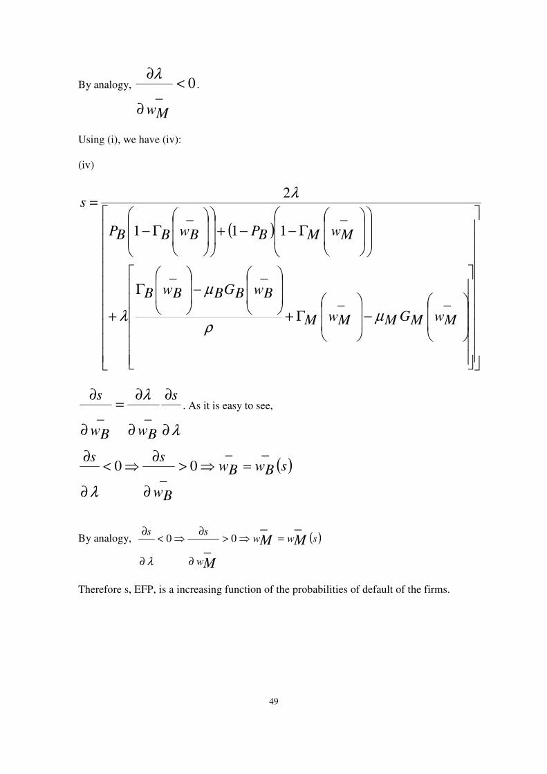
49

By analogy, 0_

<

∂

∂

Mw

λ.

Using (i), we have (iv):

(iv)

( )

−

Γ+

−

Γ

+

Γ−−+

Γ−

=

__

__

_11

_1

2

MwMGMMwM

BwBGBBwB

MwMBPBwBBP

s

µρ

µ

λ

λ

λ

λ

∂

∂

∂

∂=

∂

∂ s

BwBw

s

__. As it is easy to see,

( )sBwBw

Bw

ss__

0_

0 =⇒>

∂

∂⇒<

∂

∂

λ

By analogy, ( )sww

w

ssMM

M

__

_00 =⇒>

∂

∂⇒<

∂

∂

λ

Therefore s, EFP, is a increasing function of the probabilities of default of the firms.

50

Proposition 2

Given the structure of the model described above and in the text, the external finance

premium, EFP, is a decreasing function of the probability of the firm to obtain a loan at

BNDES if the expected profit of BNDES is less than the expected profit of the market

lender.

From (iv) above, we have:

0

112

2[]

__

<

Γ−−

Γ−−

=∂

∂

MMBB

B

ww

P

s

λ

:

Where [] is the denominator of (iv)

Γ<

Γ⇔<

∂

∂ __0 MwMBwB

BP

s

the external finance premium in brazil: empirical … · analyses using state space models fernando...

Documents