the expectations trap hypothesis
TRANSCRIPT

ighto
from
ghthat
lsoin
aryandducellen
e
areionscall
ursthe
Introduction and Summary
Many countries, including the United States, experienced a costly, hinflation in the 1970s. This article reviews some research devotedunderstanding why it happened and what can be done to prevent ithappening again.
We take it for granted that the high inflation was the result of himoney growth produced by the U.S. Federal Reserve. But, to make sureit does not happen again, it is not enough to know who did it. It is anecessary to knowwhy the Fed did it. We hypothesize that the Fed waseffect pushed into producing the high inflation by a rise in the inflationexpectations of the public. In the language of Chari, Christiano,Eichenbaum (1998), we say that when a central bank is pressured to proinflation because of a rise in inflation expectations, the economy has fainto an expectations trap. We call this hypothesis about inflation thexpectations trap hypothesis.
We argue that the dynamics of inflation in the early 1970sconsistent with the expectations trap hypothesis. We describe two versof this hypothesis. We also describe an alternative hypothesis, which wethe Phillips curve hypothesis. According to this hypothesis, inflation occwhen a central bank decides to increase money growth to stimulate
The Expectations Trap Hypothesis
Lawrence J. Christiano and Christopher Gust
347
* This is a later version of the paper presented, under the title “The Great Inflation of the1970s,” at the conference. It is also published in the Federal Reserve Bank of Chicago’sEconomic Perspectives, Second Quarter 2000, 25 (2): 21–39.The authors have benefited from discussions with Martin Eichenbaum. Lawrence Christianois grateful for the support of a grant from the National Science Foundation to the NBER.

348 Christiano and Gust
ils.bothere
tionthising asonstrapralltheoff
inyalí,singriousctedionthe
f the
thethe
onLMt isriseiated-thel.’sest,
vans
ingpolicytion
economy and is willing to accept the risk of high inflation that that entaThe expectations trap hypothesis and the Phillips curve hypothesismaintain that high inflation is a consequence of high money growth. Whthey differ is in the motives that they ascribe to the central bank.
Much of our analysis assessing the various hypotheses about inflais based on an informal review of the historical record. We supplementdiscussion by studying a version of the expectations trap hypothesis usgeneral-equilibrium, dynamic macroeconomic model. There are two reathat we do this. First, we want to demonstrate that the expectationshypothesis can be integrated into a coherent view of the ovemacroeconomy.1 Second, we want to document that that hypothesis haspotential to provide a quantitatively realistic account for the 1970s takein inflation.
The model we use is the limited-participation model studiedChristiano and Gust (1999).2 It requires a specification of monetary policin the 1970s, and for this we use the policy rule estimated by Clarida, Gand Gertler (1998). The account of the early 1970s that we produce uthe model posits that a bad supply shock (designed to capture the vacommodity shortages of the early 1970s) triggered a jump in expeinflation, which then became transformed into higher actual inflatbecause of the nature of monetary policy. We find that, consistent withdata, the model predicts stagflation. We view this result as supportive oexpectations trap hypothesis.
We compare our model with an alternative quantitative model of1970s inflation proposed by Clarida et al. That model can also explainrise in inflation in the 1970s as reflecting a self-fulfilling increase in inflatiexpectations. It is a sticky-price, rational-expectations version of the IS-model.3 When we use that model to simulate the 1970s, we find that iinconsistent with the observed stagflation of the time. It predicts that thein expected and actual inflation triggered by a bad supply shock is assocwith a sustainedrise in employment. We conclude that the limitedparticipation model provides a better account of the high inflation of1970s than does the sticky-price, IS-LM model with Clarida et arepresentation of policy. This result is potentially of independent intersince the latter model is currently in widespread use.
1. Also, see Chari, Christiano, and Eichenbaum (1998).2. This model is a modified version of the model in Christiano, Eichenbaum, and E(1998).3. The model is derived from a dynamic general-equilibrium model with maximizagents and cleared markets. The possibility that such a model could, under the sort ofestimated by Clarida et al. using data from the 1970s, have an equilibrium in which inflaexpectations can be self-fulfilling was first discovered by Kerr and King (1996).

The Expectations Trap Hypothesis 349
andide
urvetrap
hen
henat is
nts’ctualen.by anpensrtainan
tualthatwellan
ifferionsntednalre
andasedtheyputs
ite—
We begin with a description of the expectations trap hypothesiswhat it implies for policy. Then, we review the 1960s and 1970s and provan informal assessment of the expectations trap and Phillips chypotheses. We provide a quantitative evaluation of the expectationshypothesis using the limited-participation model as a vehicle. We tprovide an assessment of the Clarida et al. model.
1 What Is an Expectations Trap?
We begin with an abstract definition of an expectations trap. We tdescribe two particular types of expectations traps. Finally, we ask, Whthe ultimate cause of inflation under the expectations trap hypothesis?
1.1 The trap, defined
An expectations trap is a situation in which an increase in private ageexpectations of inflation pressures the central bank into increasing ainflation.4 There are different mechanisms by which this can happHowever, the basic idea is always the same. The scenario is initiatedrise in the public’s inflation expectations. Exactly why their inflatioexpectations rise doesn’t really matter. What does matter is what hapnext. On the basis of this rise in expectations, private agents take ceactions which then place the Fed in a dilemma: either respond withaccommodating monetary policy which then produces a rise in acinflation or refuse to accommodate and risk a recession. A central bankis responsive to concerns about the health of the economy could verywind up choosing the path of accommodation, that is, falling intoexpectations trap.
1.2 A cost-push trap and a working capital trap
We describe two versions of the expectations trap hypothesis, which daccording to the precise mechanism by which higher inflation expectatpressure the Fed into supplying more inflation. One mechanism, presein Chari, Christiano, and Eichenbaum (1998), is similar to the conventiocost-pushtheory of inflation. We call it a cost-push expectations trap. Heis how it works. Higher inflation expectations lead people to demand,receive, higher wage settlements. Firms are happy to pay the increwages because, expecting a rise in the general price level, they thinkcan pass along the higher wage costs in the form of higher prices. This
4. In this paper, we focus on expectations traps in which inflation is high. The opposan expectations trap in which inflation is low—is also a possibility.

350 Christiano and Gust
ationthell notceionsion
esis0s.have
w,cur.
onderderct onhowtionk is
t thehisratesma.tion
esttlyf thee int ofnd
as an
the Fed in the dilemma mentioned above. The Fed can produce the infleveryone expects by raising money growth. Or, if it does not, it will puteconomy through a recession. Under some circumstances, the Fed wibe willing to tolerate the recession and will feel compelled to produinflation. In this case, the Fed ends up validating the original rise in inflatexpectations. We call this hypothesis about inflation, the cost-push verof the expectations trap hypothesis.5
We shall see that this version of the expectations trap hypothencounters some difficulties explaining the high inflation of the 197We now describe another version of this hypothesis, which does notthese problems.
The limited-participation model of money, which is analyzed belohighlights a different mechanism by which an expectations trap can ocWe call this aworking-capitalexpectations trap. It relies on the assumptithat firms must borrow funds in advance (acquire working capital) in orto finance some or all of the inputs needed to carry on production. Unthese circumstances a high nominal interest rate has a negative impaeconomic activity because it raises the cost of working capital. To seethis mechanism works, suppose, again, that there is a jump in inflaexpectations. Private agents, correctly perceiving that the central banafraid of the negative output effects of high interest rates, anticipate thahigher future inflation will be associated with low real interest rates. Tleads them to cut back on saving, putting upward pressure on interestin the market for loanable funds. This places the central bank in a dilemIf it keeps the money supply unchanged, then the higher expected inflawill not occur. However, the reduced saving would result in high interrates. By drying up the supply of working capital, this would significanslow the economy. A central bank that is concerned about the health oprivate economy may prefer a second option: prevent a substantial risinterest rates by injecting money into the economy. This has the effecvalidating the initial jump in inflation expectations. Choosing this seco
5. The cost-push expectations trap is very close to the hypothesis Blinder advancesexplanation of the takeoff of inflation in the early 1970s:
Inflation from special factors can “get into” the baseline rate if it causes anacceleration of wage growth. At this point policymakers face an agonizingchoice—the so-called accommodation issue. To the extent that aggregatenominal demand isnot expanded to accommodate the higher wages andprices, unemployment and slack capacity will result. There will be arecession. On the other hand, to the extent that aggregate demandisexpanded (say, by raising the growth rate of money above previoustargets), inflation from the special factor will get built into the baselinerate. (Blinder 1982, 264)

The Expectations Trap Hypothesis 351
hisons
ate
rapfor
ine ase innly
ightriousen athatriceshebersontsidethe
n tothatin
thatvenFore ofre amictrap
ionps,nt topleoutt.
option is another way to fall into an expectations trap. We call thypothesis about inflation the working-capital version of the expectatitrap hypothesis.
1.3 Ultimate cause of inflation
Where, under the expectations trap hypothesis, does the ultimresponsibility for inflation lie? To answer this requires identifying thecauseof the rise in inflation expectations. According to the expectations thypothesis, the cause lies with monetary institutions themselves. If,example, the nature of those institutions is such that people cannot imagset of circumstances in which the central bank would accommodate a riinflation, then there is little reason for inflation expectations to suddejump. Expectations traps just couldn’t happen.
To see this, imagine there is an oil shortage. Certainly, one mreasonably expect this to lead to a rise in the price level. Because of valags, this rise might actually take place over a period of time, maybe evyear or two. But, there is nothing in conventional economic reasoningwould connect an oil shortage to the sustained, decade-long rise in pthat we call inflation. Anyone who inferred from a 10 per cent jump in tprice level in one year that prices would continue jumping like this and100 per cent higher in ten years, would be viewed as a crank. Such a pewould seem as foolish as the person who, seeing the temperature oudrop one degree from one day to the next, forecasts a drop intemperature by 100 degrees over the next 100 days.
Now consider an economy whose monetary institutions are knowassign a high priority to output and employment. In addition, supposethat economy’s central bank has no way of credibly committing itselfadvance to keeping money growth low. In a society like this, the ideainflation could take off seems quite plausible. In such a society, eseemingly irrelevant events could spark a rise in inflation expectations.example, a person who revised upward their inflation forecast in the wakan oil shock would now not necessarily seem like a crank. There anumber of ways they could back up their forecast with sensible econoreasoning. Such a person could use either of the two expectationsarguments described above.
So, the expectations trap hypothesis lays responsibility for inflatwith monetary institutions. To reduce the possibility of expectations trathe institutions must be designed so that the central bank’s commitmefighting inflation is not in doubt. Under these circumstances, peoparticipating in wage negotiations who profess to believe inflation is abto take off will be met with disbelief rather than a higher wage settlemen

352 Christiano and Gust
thet onleast
f the(or
Alanech,cectedong.t on
thatomy,
theh therap by
traphatsary,the
atathe
heationthe
l ofianer
obin.theility
).
How exactly monetary institutions should be designed to reducelikelihood of an expectations trap is controversial. But, there is one poinwhich there appears to be agreement. The central banker at the veryshould make a show of not being too concerned about the health oeconomy. An example of this can be found in the reaction to a famousinfamous) speech by the then vice-chairman of the Federal Reserve,Blinder, at a conference in Jackson Hole, Wyoming, in 1994. In that speBlinder acknowledged that it is feasible for a central bank to influenunemployment and output. This generated an uproar. Many who objeprobably did not do so because they thought what Blinder said was wrInstead, they simply thought it unwise that a central banker should lethat he thinks about such things.6 Why shouldn’t he let on? Onepossibility—the one emphasized in the expectations trap hypothesis—isthe greater the apparent concern by the central bank for the real econthe greater is the risk of falling into an expectations trap.
2 Background Events
We provide a brief review of the basic economic events leading up tohigh inflation of the 1970s. We argue that the data appear consistent withypothesis that the United States became ensnared in an expectations tthe late 1960s and early 1970s. We then compare the expectationshypothesis about inflation with another hypothesis. According to thypothesis, the Fed consciously produced the high inflation as a necesthough unfortunate, by-product of its aggressive attempts to stimulateeconomy. We call this thePhillips curve hypothesis, because it involvesthe Fed’s attempts to exploit the Phillips curve. Finally, we look at the dto identify the economic consequences of the takeoff in inflation inearly 1970s.
2.1 Events leading up to the 1970s: Setting the trap
An important part of the story of the inflation of the 1970s begins with trecession of the early 1960s. That recession helped bring the administrof John F. Kennedy into power. Kennedy brought with him the best andbrightest Keynesian minds of the time. The chairman of the CounciEconomic Advisers (CEA) was the very distinguished Keyneseconomist, Walter Heller. Members of the CEA included anothdistinguished Keynesian economist, the future Nobel laureate, James TGovernment policy was animated by the Keynesian conviction that ifeconomy was performing below its potential, then it was the responsib
6. For one prominent commentator who takes this position, see Barro (1996, 58–60

The Expectations Trap Hypothesis 353
d toowthears
aded
alsos ofthehe
rs’isest
encee ahe
oneThey-te in70nuedre 1).in a
ingsee theined
, and
x with
of the government to use the fiscal and monetary policies at its commanrestore it to strength. Figure 1 displays the federal funds rate and the grrate of the monetary base, using annual data. Also exhibited are the ydesignated by the NBER to be periods of business cycle contraction (sharea) and expansion (non-shaded area).7 The figure shows that the growthrate in the monetary base began to pick up in the early 1960s. The CEAset to work to craft an expansionary fiscal policy, and one of the productthose efforts was the tax reduction legislation of 1964. Confidence infeasibility and desirability of Keynesian stabilization policy soared with tlong expansion of the 1960s.
Figure 2 shows that inflation started to pick up with a few yeadelay, in 1965.8 As these observations suggest, that initial rise in inflationprobably not an example of an expectations trap. It is probably bunderstood in terms of the Phillips curve hypothesis: It was the consequof expansionary monetary policy, deliberately undertaken to stimulatweak economy. It is the dynamics of inflation after the initial uptick in t1960s that appears to take on the character of an expectations trap.
Figures 1 and 2 show that inflation proceeded to hit three peaks,in the early 1970s, one in early 1975, and the final one in late 1980.initial pickup in inflation in the 1960s was noted with alarm by policmakers, who responded with a very sharp rise in the federal funds ra1969. This policy tightening is often credited with producing the 19recession. Policy-makers expressed dismay that the inflation rate contito be high, even as the economy began to slide into recession (see FiguArthur Burns, the chairman of the Federal Reserve at this time, saidspeech at Pepperdine College, Los Angeles, on 7 December 1970:
The rules of economics are not working in quite the way theyused to. Despite extensive unemployment in our country, wagerate increases have not moderated. Despite much idleindustrial capacity, commodity prices continue to rise rapidly.(Burns 1978, 118)
The policy establishment became convinced that the underlydriving force of inflation was inflation expectations and that theexpectations were all but impervious to recession. In a statement beforJoint Economic Committee of the U.S. Congress in 1971, Burns explathe role of inflation expectations as follows:
7. The data are taken from Citibase. The mnemonic for the federal funds rate is fyffthe mnemonic for the monetary base is fmbase.8. Inflation is measured as the annual per cent change in the consumer price indeCitibase mnemonic, prnew (CPI-W: all items).

354 Christiano and Gust
Figure 1Base growth and federal funds rate
Figure 2Base growth and inflation
20
15
10
5
0
−5
1955 ’60 ’65 ’70 ’75 ’80 ’85 ’90
Rate
Basegrowth
Annual average per cent
Note: Shaded areas indicate NBER-dated recessions.Source: Based on data from Citibase.
15
10
5
0
−5
1955 ’60 ’65 ’70 ’75 ’80 ’85 ’90
Basegrowth
Inflation
Annual average per cent
Notes: Shaded areas indicate NBER-dated recessions.Inflation is measured as the annual per cent change in the CPI with Citibase mnemonic,prnew(CPI-W: all items).Source: Based on data from Citibase.

The Expectations Trap Hypothesis 355
berebe
tives,
e of70,wthght
e on
Consumer prices have been rising steadily since 1965—muchof the time at an accelerating rate. Continued substantialincreases are now widely anticipated over the months andyears ahead. . . . [I]n this environment, workers naturally seekwage increases sufficiently large . . . to getsome protectionagainst future price advances. . . . [T]houghtful employers . . .reckon, as they now generally do, that cost increases probablycan be passed on to buyers grown accustomed to inflation.(Burns 1978, 126)
Policy-makers understood that, in principle, inflation couldstopped with a sufficiently restrictive monetary policy, but they weconcerned that the short-run costs, in terms of lost output, wouldintolerable. In an appearance before the House of RepresentaCommittee on Banking and Currency, 30 July 1974, Burns said:
One may therefore argue that relatively high rates of monetaryexpansion have been a permissive factor in the acceleratedpace of inflation. I have no quarrel with this view. But an effortto use harsh policies of monetary restraint to offset theexceptionally powerful inflationary forces of recent yearswould have caused serious financial disorder and economicdislocation. That would not have been a sensible course formonetary policy. (Burns 1978)
In remarks before the Seventeenth Annual Monetary Conferencthe American Bankers Association, Hot Springs, Virginia, 18 May 19Burns elaborated on his views about the costs of relying on money groalone (without, say, wage and price controls) to reduce inflation. He thouthe costs were so large that the strategy was fundamentally infeasiblpolitical grounds. In his words,
There are several reasons why excessive reliance on monetaryrestraint is unsound. First, severely restrictive monetarypolicies distort the structure of production. General monetarycontrols, despite their seeming impartiality, have highlyuneven effects on different sectors of the economy. On the onehand, monetary restraint has relatively slight impact onconsumer spending or on the investments of large businesses.On the other hand, the homebuilding industry, state and localconstruction, real estate firms, and other small businesses arelikely to be seriously handicapped in their operations. Whenrestrictive monetary policies are pursued vigorously over aprolonged period, these sectors may be so adversely affectedthat the consequences become socially and economically

356 Christiano and Gust
ting71
o theneypageons.ageemsrice
eyrice
angerwas
ce of
ntaydot
5 per
ney
intolerable, and political pressures mount to ease up on themonetary brakes. . . .
An effort to offset, through monetary and fiscal restraints, allof the upward push that rising costs are now exerting on priceswould be most unwise. Such an effort would restrict aggregatedemand so severely as to increase greatly the risks of a veryserious business recession. If that happened, the outcries of anenraged citizenry would probably soon force the governmentto move rapidly and aggressively toward fiscal and monetaryease, and our hopes for getting the inflationary problem undercontrol would then be shattered. (Burns 1978)9
Policy-makers were so pessimistic about the prospects of getinflation under control by restrictive monetary policy, that in August 19they turned to wage and price controls.
What happened after this may seem to be an embarrassment texpectations trap hypothesis, particularly the cost-push version: Mogrowth continued to be high.10 According to the cost-push expectations trahypothesis, high money growth is the Fed’s response to inflationary wand price contracts, which are themselves driven by inflation expectatiBut, inflationary wage and price contracts became illegal during the wand price control period, which lasted until 1973. So, this hypothesis seto predict that money growth would have been low during the wage-pcontrols, not high.11
The key to reconciling the expectations trap with this high mongrowth lies in interest rates. Policy-makers were convinced that wage-p
9. In the same speech, Burns showed some foresight in warning about another dassociated with the strategy of relying on reduced money growth to stop inflation. Heconcerned that the nature of the lags in monetary policy was such that the varianinflation and money growth would go up in a “stop-and-go” process.
[T]he effects of monetary restraint on spending often occur with relatively longlags. . . .Because the lags tend to be long, there are serious risks that a stabilizatioprogram emphasizing monetary restraint will have its major effects on spending aa point in time when excess demand has passed its peak. The consequence mthen be an excessive slowdown of total spending and a need to move quickly anaggressively toward stimulative policies to prevent a recession. Such a stop-and-gprocess may well lead to a subsequent renewal of inflationary pressures of yegreater intensity. (Burns 1978)
10. Money growth in 1970–74 was 5.32 per cent, 7.60 per cent, 7.27 per cent, 8.7cent, and 7.99 per cent, respectively. The number for periodt is 100 x log
, wherem(t) denotes the monetary base,t = 1970, 1971, 1972, 1973,and 1974.11. We address the potential for the Phillips curve hypothesis to explain high mogrowth during the period of wage-price controls in the next subsection.
m t( )/m t 1–( )( )

The Expectations Trap Hypothesis 357
toas
s tohisandthetaryongn is
ing-esisoliothe
oneythe
heyoff.rateshownerely
le ofatedin thes ofeen
s and
ver,r Warctediod ofectednite
ast ofralthe
n realGDP
controls would not be politically feasible if interest rates were alloweddrift up. They thought that if this happened, the controls would be vieweda cover for redistributing income from people earning wages and salariethe (typically wealthy) people who earn interest. They feared that if thappened, then political support for the controls would evaporate,inflation would take off again. So, policy was directed toward keepingnominal interest rate about where it was before the severe monetightening of 1969 (see Figure 3). It is interesting that it required such strmoney growth to keep the interest rate at this level. A possible explanatiothat this reflects the type of portfolio decisions emphasized in the workcapital expectations trap hypothesis described earlier. That hypothpredicts that, in the absence of high money growth, household portfdecisions motivated by concerns about future inflation would drive uprate of interest.
These considerations suggest to us that although the high mgrowth during wage-price controls may well be an embarrassment toexpectations trap hypothesis, it isn’t necessarily so.
Policy-makers started dismantling wage-price controls in 1973. Twere once again surprised by the strength with which inflation tookThey had anticipated some inflationary pressure, and they raisedsharply in this period (see Figure 3). But, they were surprised at juststrong the rise in inflation was.12 The increase in rates was greater than omeasure of the rise in expected inflation (see Figure 3). And, it just bakept up with actual inflation (Figure 4).13 Policy-makers’ resolve began tofade when output and investment started to show weakness in the midd1973 and hours worked began to soften in late 1973. They had indicrepeatedly that they were unwilling to countenance a severe recessionfight against inflation. Their concerns about the recessionary costfighting inflation seemed credible since they appeared to have bconfirmed by the experience of the 1970 recession. Moreover, the 1960
12. To some extent, the rise in inflation was due to the oil shock in late 1973. Howeabout three-quarters of the price increases of that year occurred before the Yom Kippuand the October oil embargo. The takeoff in inflation in 1973 may, in part, have reflethe delayed response of prices to the high money growth that occurred during the perwage-price controls. We attempted to estimate what fraction of the 1973 price rise reflpast money growth, but found that statistical uncertainty is too large to draw a deficonclusion.13. We calculated expected inflation for Figure 4 based on a 1-month-ahead forecmonthly CPI inflation using 5-month lags in monthly inflation, 4-month lags in the fedefunds rate, 4-month lags in the monthly growth rate in M2, and 4-month lags inpremium in the return to 10-year Treasury bonds over the federal funds rate. The rise irates reported in Figures 4 and 5 would have been somewhat larger if we had used thedeflator to measure inflation.

358 Christiano and Gust
Figure 3Federal funds rate and inflation
Figure 4Ex ante real rate
20
15
10
5
0
−5
1955 ’60 ’65 ’70 ’75 ’80 ’85 ’90
Annual average per cent
Note: Shaded areas indicate NBER-dated recessions.Source: Based on data from Citibase.
Rate
Inflation
12
8
4
0
−4
1962 ’66 ’70 ’74 ’78 ’82 ’86 ’90 ’94 ’98
Annual average per cent
Note: Shaded areas indicate NBER-dated recessions.Source: Based on data from Citibase.

The Expectations Trap Hypothesis 359
s forcialgcese of
ed athewere1975d in
ain
aryds
videdwast of
theWIIilize
licy in
ote 9.y and
1970s were times when governments were expected to do good thingtheir citizens, and hurting a subset of them for the sake of curing a soproblem seemed unfair and wrong.14 In an address before the joint meetinof the American Economic Association and the American FinanAssociation, on 29 December 1972, Burns expressed the general senthe time:
Let me note, however, that there is no way to turn back theclock and restore the environment of a bygone era. We can nolonger cope with inflation by letting recessions run theircourse; or by accepting a higher average level of unem-ployment. . . . There are those who believe that the time is athand to . . . rely entirely on monetary and fiscal restraint torestore a stable price level. This prescription has greatintellectual appeal; unfortunately, it is impractical. . . . Ifmonetary and fiscal policies became sufficiently restrictive todeal with the situation by choking off growth in aggregatedemand, the cost in terms of rising unemployment, lost output,and shattered confidence would be enormous. (Burns 1978)
So, toward late 1974, policy-makers reversed course and adoptloose monetary policy, driving interest rates down sharply, to turneconomy around. Note from Figures 4 and 5 that real interest ratesnegative or close to zero. Of course, as the economy entered the deeprecession, inflation came down substantially anyway. But, the turnarounmonetary policy then had the implication that inflation would take off agas soon as the economy entered the expansion.15 Only later, in 1978 and1979, did the Fed turn “tough” and consciously adopt a tight monetpolicy until inflation came down (see how much higher the federal fun
14. With the experience of the Great Depression and the intellectual foundations proby Keynes’ General Theory, it was generally accepted that governments’ responsibilityto preserve the health of the economy. This was put into law in the Employment Ac1946, which created the CEA:
There is hereby created in the Executive Office of the President a Council ofEconomic Advisers . . . to formulate and recommend national economic policy topromote employment, production, and purchasing power under free competitiveenterprise.
See De Long (1995) for a discussion of the post-WWII intellectual climate regardingproper role of government in the economy and the sharp contrast with the pre-Wclimate. As noted earlier, the feasibility of the notion that the government ought to stabthe economy seemed to be confirmed with the apparent success of stabilization pothe 1960s.15. This was precisely the stop-and-go process that Burns feared, as mentioned in nFor another discussion of the stop-and-go nature of inflation in this period, see BarskKilian (2000).

360 Christiano and Gust
tionte
thatan
two
le tod inwasnstionthesedonature
the
Figure 5Ex post real rate
12
8
4
0
−4
1962 ’66 ’70 ’74 ’78 ’82 ’86 ’90 ’94 ’98
Annual average per cent
Note: Shaded areas indicate NBER-dated recessions.Source: Based on data from Citibase.
rate went in the early 1980s, and note how it stayed up—with the excepof a brief period of weakness in mid-1980—until after the inflation rabegan to fall).
We interpret these observations as being consistent with the viewby the late 1960s and early 1970s, the U.S. economy had fallen intoexpectations trap. Through their words and actions, policy-makers sentclear messages to the population:
• It is technically feasible for policy-makers to stop inflation.
• The costs of doing so were greater than policy-makers could accept.
Under these circumstances, it was perhaps reasonable for peopexpect higher inflation. When wage-price controls began to be dismantle1973, it would have been reasonable for the public to think that therenow nothing left standing in the way of high inflation. Inflation expectatiowere even stronger than before. One indication of this is that actual inflatook much longer to begin falling during the 1974 recession than it did in1970 recession (see Figure 3). Ironically, while policy-makers expresfrustration with the public for the seeming intransigence of their inflatiexpectations, the true cause of that intransigence may have been the nof the monetary policy institutions themselves. This is the implication ofexpectations trap hypothesis.

The Expectations Trap Hypothesis 361
f inrapt it
h. Itsetatesveivelypear
ntialterly
tothe
gingDP
eenundntialote
s ofls is7.
DP.205)s thisrdennly
erald
e, theich,nearr cann andes, itted or
2.2 Phillips curve hypothesis
We now briefly consider the Phillips curve hypothesis about the takeofinflation that occurred in the early 1970s. Like the expectations thypothesis, this hypothesis is also fundamentally monetarist in thainterprets the rise in inflation as reflecting an increase in money growtdiffers from the expectations trap hypothesis by highlighting a differentof motives on the part of the Fed. Policy-makers believed the CEA estimthat output was below potential in 1971. Under the Phillips curhypothesis, the Fed responded to this by adopting an aggressexpansionary monetary policy for the same sort of reasons that they apto have done so in the early 1960s, to restore output and employment.
To see that the economy was below at least one measure of potein 1971, consider the results in Figures 6 and 7. Figure 6 displays quardata on (log) real GDP in the United States for the period 1966Q11973Q4. In addition, we report two estimates of potential GDP based onHodrick and Prescott (1997) filter.16 One is computed using data coverinthe period, 1948Q1–1998Q1. A possible problem with this is that by uscurrently available data we may overstate the estimate of potential Gavailable to policy-makers in the early 1970s. They would not have baware of the slowdown in trend (that is, potential) GDP that started arothat time (Orphanides 1999). This motivates our second estimate of poteoutput, which is based only on data for the period 1948Q1–1973Q4. Nfrom Figure 6 that the qualitative difference between the two estimatepotential is as expected. However, quantitatively, the difference in levequite small. The implied estimates of the output gap appear in Figure17
16. The trend implicit in the H-P filter is a fairly standard way to estimate potential GFor example, the Organisation for Economic Co-operation and Development (1999,reports estimates of the output gap computed in this way. Taylor (1999a) also usemethod to compute the output gap. Finally, according to Orphanides and van No(1999, 1), “The difference between [actual output and potential output] is commoreferred to as thebusiness cycle or the output gap[italics added].” For an analysis of thestatistical properties of this way of computing the output gap, see Christiano and Fitzg(1999).
There are other output-gap measures based on a different notion of trend. In thestrend corresponds to the “non-accelerating inflation” level of the variable: the level whif it occurred, would produce a forecast of zero change in the rate of inflation in thefuture. Gap concepts like this are fundamentally multivariate. To see how the H-P filtebe adapted to correspond more closely to this alternative gap concept, see LaxtoTetlow (1992) and St-Amant and van Norden (1997). We assume that, for our purposdoes not matter significantly whether the output gap is measured based on the adjusunadjusted versions of the H-P filter.17. The output gap is measured as 100 x (logGDP – logGDPtrend), where logGDPtrend isthe trend in log GDP implied by the H-P filter.

362 Christiano and Gust
Figure 6Real GDP and two measures of potential GDP
Figure 7Two measures of GDP gap
8.3
8.2
8.1
8.0
7.9
1966 ’67 ’68 ’69 ’70 ’71 ’72 ’73 ’74
Source: Based on data from Citibase.
Per centLog GDPPotential ’73Potential ’98
............
4.0
0.0
−4.0
−8.0
1948 ’58 ’63 ’68 ’73’53
Annual average per cent
Source: Based on data from Citibase.
Gap ’98Gap ’73

The Expectations Trap Hypothesis 363
then971
e 7).a
ieffor
inlysingionort-
d byfor
ing
anseslemthe
pastand
hatarlyreal
nd
rve.was,. See
Note that the two sets of estimates virtually coincide through 1970, anddiverge a little after that. Each estimate implies that the gap in 1averaged around 2 per cent.18
The 2 per cent gap was substantial by historical standards (FigurStill, the notion that policy-makers actively solicited higher inflation asway to fight a weak economy conflicts sharply with the words of the chmonetary policy-maker, Burns. Burns was very clear about his distasteexploiting the Phillips curve for the sake of short-term gains. He certaaccepted the notion that policy could achieve higher output by increainflation. After all, his fears about the consequences of fighting inflatwith reduced money growth were fundamentally based on a belief in a shterm Phillips curve. His view, which corresponded to the one espouseMilton Friedman (1968), was that attempts to exploit the Phillips curveshort-term gains would only produce more trouble in the long run.19 As heput it in testimony before Wright Patman’s House Committee on Bankand Currency, 30 July 1974:
We have also come to recognize that public policies that createexcess aggregate demand, and thereby drive up wage rates andprices, will not result in any lasting reduction inunemployment. On the contrary, such policies—if longcontinued—lead ultimately to galloping inflation, to loss ofconfidence in the future, and to economic stagnation.(Burns 1978, 170)
It is hard to doubt the sincerity of these words. To Burns,important lesson of the inflation of the 1970s was that price increaproduced by temporary forces could lead to an intractable inflation problater on. It would have taken an extraordinary amount of duplicity to, onone hand, complain about the serious economic damage caused bypolicy mistakes in not counteracting temporary forces, and on the other hcontribute to them himself.20
2.3 Springing the trap
To evaluate our models, we require a simple characterization of whappened when the economy fell into the expectations trap in the e1970s. For this, consider Figures 8–10, which display the logarithm of
18. The average gap for 1971 was−1.75 per cent according to the full sample estimate a−1.99 per cent according to the sample that stops in 1973Q4.19. See Wells (1994, 72) for a further discussion of Burns’ view about the Phillips cu20. It has been argued that even if Burns was not himself duplicitous, President Nixonand Burns acted at the behest of Nixon. To us, the record is inconsistent with this viewthe appendix.

364 Christiano and Gust
Figure 8Gross domestic product and trends
Figure 9Hours of all persons, business sector, and trends
9.4
8.8
8.2
7.6
7.0
1948 ’53 ’58 ’63 ’68 ’73 ’78 ’83 ’88 ’93 ’98
Source: Based on data from Citibase.
LogarithmRaw dataTrend ’70sTrend pre-’70Quadratic............
4.8
4.6
4.4
4.2
4.0
1948 ’53 ’58 ’63 ’68 ’73 ’78 ’83 ’88 ’93 ’98
Source: Based on data from Citibase.
Logarithm
Raw dataQuadraticTrend pre-’70............

The Expectations Trap Hypothesis 365
xedted
latedrendn, in
lsothe
two70sfromthat
mustteatedes.thearlyentuseath.ssion.97.
Figure 10Business fixed investment and trends
7.5
7.0
6.5
6.0
5.5
5.0
1948 ’53 ’58 ’63 ’68 ’73 ’78 ’83 ’88 ’93 ’98
LogarithmRaw dataQuadraticTrend pre-’70
Source: Based on data from Citibase.
............
GDP, total hours worked in nonagricultural business, and business fiinvestment, respectively. In addition, we display linear trends, compuusing the data from the beginning of the sample to 1970Q1, and extrapothrough the end of the sample. These lines draw attention to the tchange that occurred in these variables in the early 1970s. In additioeach case we also fit a quadratic trend to the entire sample of data.
Consider the GDP data in Figure 8 first. In this case, we have aincluded a linear trend fit to the data for the 1970s and extrapolated toend of the sample. What is clear, by comparing the raw data with thelinear trends, is that the growth slowdown that started in the early 19became even more severe in the 1980s and the early 1990s. We inferthe fact that the slowdown persisted—even accelerated—in this period,the inflation and other transient shocks that occurred in the early 1970shave had little to do with it. Now consider hours worked in Figure 9. Nohow they take off beginning in the early 1970s, and how the growth rseems to just increase continuously throughout the following decaAgain, we infer from the fact that the growth rate continued to rise afterinflation stopped that the inflation and other temporary factors in the e1970s were not a factor in this development. Finally, note that investmshows very little trend change in the 1970s (see Figure 10). After a paduring the 1974–75 recession, investment returns to its former growth pInvestment does display weakness in the late 1980s and the 1990 receBut after that, it grows again, returning to the pre-1970s trend line by 19

366 Christiano and Gust
our70s.
torshaveraticts ofarell toutputt inwentend
g up
rapy theomyitedce,
ed’sHestateomlicy
f itsits
he
l in
These trend changes in hours worked and output complicateattempts to assess alternative explanations of the inflation of the 19Ideally, we would like to remove the effect on the data reflecting the facunderlying the persistent change in trend, and study the remainder. Wenot found a clean way to do this. The approach we take removes a quadtrend from each variable and assumes that the result reflects the effecthe inflation and bad supply shocks of the early 1970s. The resultsdisplayed in Figures 11–13. In the 1974–75 recession hours worked fearound 6 per cent below trend, investment was down 11 per cent, and owas down 3 per cent. At the same time, inflation rose from 4 per cen1972 to 10 per cent by the end of the recession. The federal funds ratefrom around 4 per cent in 1972 to a peak of around 12 per cent near theof the recession. The episode is a classic stagflation, with inflation goinand the economy, down.
3 Models
We now report on a quantitative evaluation of the expectations thypothesis. For this, we need a mathematical representation of the wacentral bank conducts monetary policy and of the way the private econis put together. We describe two models of the private economy: the limparticipation model of Christiano and Gust (1999) and the sticky-priIS-LM model of Clarida et al.21
3.1 Monetary policy rules
There is widespread agreement that the right way to model the Fmonetary policy is along the lines proposed by Taylor (1993, 1999b).posits that the Fed pursues an interest rate target, which varies with theof the economy. A version of this policy rule was estimated using data frthe 1970s by Clarida et al. They estimated that the Fed’s monetary pocauses the actual federal funds rate, , to evolve as follows:
. (1)
In words, is a weighted average of the current target value, , and ovalue in the previous period. By setting , the Fed would achievetarget, in each period. It might instead prefer ifexhibits more volatility than it wishes to see in the actual funds rate. Ttarget interest rate is determined according to the following expression:
21. The limited-participation model that we use is a modified version of the modeChristiano, Eichenbaum, and Evans (1998).
Rt
Rt ρRt 1−ρ( )Rt*+=
Rt Rt*
ρ 0=Rt Rt
*= 0 ρ 1< < Rt*

The Expectations Trap Hypothesis 367
Figure 11Detrended hours and inflation
Figure 12Detrended investment and inflation
16
12
8
4
0
−4
−8
1948 ’53 ’58 ’63 ’68 ’73 ’78 ’83 ’88 ’93 ’98
Note: Shaded areas indicate NBER-dated recessions.Source: Based on data from Citibase.
Per cent
Inflation
Hours
20
10
0
−10
−20
Per cent
1948 ’53 ’58 ’63 ’68 ’73 ’78 ’83 ’88 ’93 ’98
Note: Shaded areas indicate NBER-dated recessions.Source: Based on data from Citibase.
InflationInvestment

368 Christiano and Gust
Theuse
owt is
70s.very
, hethe
As autputtion,
riables
thats are. point
Figure 13
Detrended output and inflation
15
10
5
0
−5
−10
1948 ’53 ’58 ’63 ’68 ’73 ’78 ’83 ’88 ’93 ’98
Note: Shaded areas indicate NBER-dated recessions.Source: Based on data from Citibase.
Inflation
Output
Per cent
, (2)
where is the price level, is the date conditional expectation, andis the per cent deviation between actual output and trend output.estimated values of , and are 0.75, 0.8, and 0.44, respectively. Wethese parameter values in our analysis.22
The idea is that a tough central banker who is committed to linflation would adopt a rule with a large value of . A central banker tha
22. Clarida et al. (1998) use revised data to estimate the policy rule for the 19Orphanides (1997) argues that constructing using final revised data may give adifferent view of than policy-makers in the 1970s actually had. As noted aboveargues that the productivity slowdown that is thought to have occurred beginning inearly 1970s was not recognized by policy-makers until much later in that decade.result, according to Orphanides, real-time policy-makers in the 1970s thought that owas further below potential than current estimates suggest. In private communicaOrphanides has informed us that when he uses real-time data on and the other vato redo the Clarida et al. estimation procedure, he finds that the point estimated forρ, α, andβ for the 1970s change. They move into the region where our models no longer implyself-fulfilling inflation takeoffs are possible. The standard errors on the point estimatelarge, however, and a standard confidence interval does not exclude the Clarida et alestimates that we use.
Rt* constant αEt πt 1+( ) γ yt πt 1+,+log+
Pt 1+
Pt------------= =
Pt Et t yt
ρ α, γ
ytyt
yt
α

The Expectations Trap Hypothesis 369
eting
y istion.iderablythed onzero.hisat a
uttherewasav-
Thein
eluceialtheThe
n. Aandirence
to arizeationthe
heirg auretheidity
less able to commit to low inflation would have a low value of . Claridaal.’s estimate for the 1970s is relatively low. The value they estimate usdata after 1979 is higher, and this is a period when monetary policthought to have been characterized by greater commitment to low inflaTo see how much tougher monetary policy became in 1979, consFigures 4, 5, and 14. Figures 4 and 5 show that the real rate was noticehigher in this period. Figure 14 exhibits the difference between whatfederal funds rate actually was and what it was predicted to be baseequation (1). Up until 1979, these differences were on average close toAfter 1979, the average shifts up noticeably (see the horizontal line). Tindicates that the actual funds rate in that period was higher than whpolicy-maker following the pre-1979 rule would have allowed.
How well does this policy rule capture our observations abomonetary policy in the 1970s? In one sense, it misses. We saw thatwere times when the Fed was very tough, and other times when itaccommodating. We think of this policy rule as capturing the Fed’s behiour on average. On average, it was accommodating.
3.2 Two models of the private economy
We now present a brief description of the models used in the analysis.mathematical equations characterizing both models may be foundChristiano and Gust (1999).
Consider the limited-participation model first. Recall that this modemphasizes a working-capital channel in the firm sector: In order to prodoutput in a given period, firms must borrow funds from the financintermediary. By increasing and decreasing its injections of liquidity,central bank can create an abundance or scarcity of those funds.resulting interest rate fluctuations then have a direct impact on productioscarcity of funds in the financial intermediary drives up the interest rateinduces firms to cut back on borrowing. With fewer funds with which to hfactors of production, they cut back on production. Similarly, an abundaof funds leads to a fall in the interest rate and an expansion of output.
The mechanism whereby a rise in expected inflation may leadrise in actual inflation in this model was sketched earlier, but we summait again here for convenience. When there is an increase in expected infl(that is, log rises) and , this translates into a decrease inreal interest rate, log . This leads households to reduce tdeposits with the financial intermediary, and has the effect of creatinscarcity of the funds available for lending to firms. Upward pressdevelops on the rate of interest. In pursuing its policy of not lettinginterest rate rise too much, the monetary authority must inject some liqu
α
Et πt+1( ) α 1<Rt Et– πt+1( )

370 Christiano and Gust
thusaryis,
tion,elf-
beourinthe
eal. Thedard
heirzes at
y’sandinto
rate
Figure 14Actual federal funds rate minus value predicted by 1970s rule
8
4
0
−4
1960 ’63 ’66 ’69 ’72 ’75 ’78 ’81 ’84
Note: Shaded areas indicate NBER-dated recessions.Source: Based on data from Citibase.
Per cent
into the banking system. This injection then produces a rise in prices,validating the original rise in inflation expectations. Since the monetauthority does permit some rise in the nominal rate of interest (that
), this has the effect of depressing output, employment, consumpand investment. Thus, the limited-participation model predicts that a sfulfilling inflation outburst is associated with stagflation.
The pure logic of the model permits an inflation outburst totriggered for no reason at all or in response to some other shock. Inmodelling exercise, we treat the jump in expectations as occurringresponse to a transitory, bad supply shock. Here, we have in mindcommodity supply shocks, including the oil shock, of the early 1970s.
Now consider the Clarida et al. model. In that model, a fall in the rrate of interest stimulates the interest-sensitive components of demandexpansion of demand raises output and employment through a stansticky-price mechanism. In particular, firms are modelled as setting tprices in advance and then accommodating whatever demand materialithe posted price. As output increases, the utilization of the economresources, particularly labour, increases. This produces a rise in coststhese are then gradually (as the sticky-price mechanism allows) passedhigher prices by firms. In this way an increase in the expected inflationgives rise to an increase in actual inflation, as long as .
α 0>
α 1<

The Expectations Trap Hypothesis 371
entonlyatedstockither
gt. Ifet al.thet thel. In
inwith
s on
g theon
se
gThat
h at in’sital
ionly
al.nd.
e ofarios
a etthislf-
otate
A feature of Clarida et al.’s model is that it does not have investmor money. The absence of investment reflects the assumption thatlabour is used to produce output. Money could presumably be incorporby adding a money-demand equation and then backing out the moneyusing output and the interest rate. Clarida et al. do not do this and nedo we.
Evidently, the Clarida et al. model implies that a self-fulfillinoutburst of inflation is associated with a rise in employment and outputhere were no other shocks in the model, then it is clear that the Claridamodel would have a problem, since it would be inconsistent withphenomenon of stagflation observed in the 1970s. However, we treaClarida et al. model in the same way as the limited-participation modeparticular, we model the jump in inflation expectations as occurringresponse to a bad supply shock. So, in principle, it might be compatiblethe low output observed in the 1970s because of the bad supply shock.
3.3 Interpreting the Taylor rule in the two models
The various hypotheses about inflation that we discuss in this paper focuthe motivesof policy-makers. The Taylor rule summarizes theirdecisions,and is silent on what motives produced these decisions. Still, in assessinlimited-participation and Clarida et al. models, it is useful to speculatewhat sort of motives might produce a Taylor rule with in themodels.
In the limited-participation model, we interpret as reflectinthe working-capital expectations trap considerations discussed above.is, in this model a rise in inflation expectations confronts the Fed witdilemma because it places the goals of low inflation and stable outpudirect conflict. An interpretation of is that this reflects the Fedrelatively greater concern for the output goal, as in the working-capexpectations trap scenario.
By contrast, in the Clarida et al. model a rise in expected inflatdoes not put the low inflation, stable output goals in conflict. By simpsayingno to high money growth and inflation, the Fed in the Clarida etmodel prevents output and inflation from simultaneously going above treSo, in the Clarida et al. model does not appear to reflect the typcentral bank dilemmas that are at the heart of the expectations trap scendescribed above. Perhaps the only interpretation of in the Claridal. model is that it reflects a mistake on the part of policy-makers. Underinterpretation, policy-makers were not aware that with , a sefulfilling inflation outburst is possible. That is, policy-makers simply did nknow that they could have gotten out of the high inflation by raising the r
α 1<
α 1<
α 1<
α 1<
α 1<
α 1<

372 Christiano and Gust
iod
ibede athe
elsntalby
nt.hey
ted-tionthe
theon-withorethisffersasedthanous
olvesl,rsds.r anymeter
of interest sharply. Our reading of the policy-making record of this permakes us deeply skeptical of this idea.23
4 Evaluating the Models
Neither of our models captures the events at the level of detail descrearlier, nor would we want them to. The question is whether we havmodel that captures the broad outlines of the takeoff in inflation in1970s.
We construct a simulation of the 1970s using the two moddescribed in the previous section. We specify that the fundameexogenous shock in this period is a shift down in the production function1 per cent.24 That is, for each level of the inputs, output falls by 1 per ceInflation expectations in the wake of this shock are not pinned down. Tare exogenous variables, like the technology shock.25 We picked theexpectations subject to two constraints. First, we required that the limiparticipation model display a long-lasting, substantial response of inflato the shock. Second, we required that the price level in the period ofproduction-function shock be the same between the two models.
23. Woodford (1998) develops an alternative interpretation of by building onassumption that fiscal policy (something we abstract from in our analysis) was “nRicardian” during the 1970s. Using the fiscal theory of the price level, he argues thatfiscal policy satisfying this condition, the Fed was forced to set to avoid an even mexplosive inflation than the one that actually occurred. For a simplified explanation ofargument, see Christiano and Fitzgerald (2000). The fiscal theory of the price level oanother potential explanation of the takeoff in inflation in the 1970s, one that is not bon self-fulfilling expectations and that assigns a central role to fiscal policy rathermonetary policy. While this interpretation is controversial, it deserves sericonsideration. See Cochrane (1998) and Woodford (1998) for further discussion.24. The production function is , where denotes gross output,denotes the stock of capital, and denotes labour. The state of technology, , evaccording to , with . In the limited-participation mode
and in Clarida et al., . The simulation involves setting foand for all othert. With this value of the state of technology remain
0.7 per cent below trend after 10 periods and 0.4 per cent below trend after 20 perio25. There is one important difference. Shocks to the production function can occur foparameter values of the model. Shocks to expectations can only exist for certain paravalues.
α 1<
α 1<
Yt zt( )KtθLt
t θ–exp= Yt KtLt zt
zt ρz zt 1– εz t,+= ρz 0.95=θ 0.36= θ 0= εzt 0.01–=t 2= εzt 0= ρz

The Expectations Trap Hypothesis 373
Figure 15Response to technology shock in two different models
12.0
8.0
4.0
0.00 3 6 9 12 15 18
Limited participation modelClarida-Galí-Gertler model
Annualized percentage rateA. Money growth
3.0
1.5
0.0
−1.5
−3.00 3 6 9 12 15 18
Per cent deviation from steady stateB. Employment
4.0
2.0
0.0
−2.0
−4.00 3 6 9 12 15 18
Annualized percentage rateC. Real interest
..........
D. ConsumptionPer cent deviation from steady state
2.0
1.0
0.0
−1.0
−2.00 3 6 9 12 15 18
15.0
10.0
5.0
0.0
E. InflationAnnualized percentage rate
0 3 6 9 12 15 18quarters
Note: Shock happens in quarter two.
1.5
0.0
−1.5
−3.00 3 6 9 12 15 18
0 3 6 9 12 15 18
F. OutputPer cent deviation from steady state
G. Nominal interestAnnualized percentage rate10.0
9.0
8.0
7.0
6.0
0 3 6 9 12 15 18
H. InvestmentPer cent deviation from steady state
2.0
0.0
−2.0
−4.0
−6.0
−8.0
I. Transactions balances (Qt)Per cent deviation from steady state15.0
10.0
5.0
0.00 3 6 9 12 15 18
quarters

374 Christiano and Gust
Theon,he
ionrest.
ds’henandositctstheill
onsadsthat
raterityofall
for aainownuse
for athanoverthes arenot
ationthe
ion ofich
odel.The
results
asizes
Consider the limited-participation model first.26 Figure 15 exhibitsthe response of the variables in that model to a bad technology shock.shock occurs in period 2. Not surprisingly, in view of our earlier discussithe shock drives output and employment down and inflation up. Tmonetary authority reacts immediately to the increase in inflatexpectations by reducing the money supply to push up the rate of inte(recall, the coefficient on expected inflation in the Taylor rule is positive)
Notice the variable, , in the model. That is the part of householfinancial wealth that they hold in the form of transactions balances. Winflation expectations go up and , then households increasecorrespondingly reduce the part of their financial wealth that they depwith financial intermediaries. The increased value of in period 3 reflehouseholds’ higher inflation expectations. They understand thatmonetary authority’s policy rule implies that the nominal rate of interest wgo up, but that it will go up by less than the increase in inflation expectati(that is, ). That is, they expect the real rate to go down. This lethem to increase the funds allocated to the goods market by raisingis, to drain funds from the financial intermediary. To guarantee that theof interest only rises by a small amount ( is small), the monetary authomust inject funds into the financial intermediary to make up for the lossfunds due to the rise in The rise in the interest rate that occurs withthis produces a fall in output and employment. The stagflation persistslong time. Money growth, inflation, and the nominal interest rate remhigh for years. Output, employment, consumption, and investment are dfor years. Investment is low, despite the low real rate of interest, becainflation acts like a tax on investment in this model.27 Note that the effectsare quite large. Output and employment remain 2 per cent below trendlong time, and money growth, inflation, and interest rates are more6 percentage points above their steady state. The fall in investment is6 per cent. Inflation rises from 4 per cent to about 10 per cent andinterest rate rises from about 7.2 per cent to 10 per cent. These resulttentative, however, since the size of the supply shock, 1 per cent, wasbased on a careful analysis of the data. Nor was the response of inflexpectations chosen carefully. Still, the results build confidence that
26. For details of model parameterization, see Christiano and Gust (1999). The versthe limited-participation model underlying the calculations in Figure 15 is the one in whinvestment is a cash good, what Christiano and Gust (1999) call the “benchmark” mThey also consider the version of the model in which investment is a credit good.simulation of the 1970s using the Clarida et al. estimated Taylor rule resembles the in Figure 15.27. Feldstein (1997) has argued that high inflation hurts investment, though he empha mechanism that operates through the explicit tax system.
Q
α 1< Q
Q
0 α 1< <Q3,
α
Q3.

The Expectations Trap Hypothesis 375
rge
g ass-orratetputced.ionwed
he
stogre isaterlow
he
el,ters,ears.riceverylogyels
) isould
ifiedrmalhari,
working-capital expectations trap hypothesis can deliver quantitatively laeffects.
What is the reason for these persistent and large effects followintechnology shock? Fundamentally, it is bad monetary policy. With a leaccommodating monetary policy, it would not be an equilibrium finflation expectations to jump so much, and so the nominal interestwould not rise so much. With a smaller interest rate rise, the negative ouand employment response to a bad technology shock would be reduFigure 16 exhibits what happens in our benchmark limited-participatmodel when the policy rule estimated by Clarida et al. to have been folloin the post-Volcker period is used.28 In this case, the equilibrium is (locally)unique.29 Note that the fall in output and employment is smaller here. Trise in the interest rate is smaller too.
We think of a small value of in the pre-Volcker policy rule areflecting that the rule is the decision of a policy-maker without an abilitycommit to low inflation. If we interpret the inability to commit as reflectinthat the policy-maker has too soft a heart for economic agents, then theplenty of irony here. The soft-hearted policy-maker in the end does gredamage to the economy than a hard-hearted one who can commit toinflation.30
Now consider the Clarida et al. model. Figure 15 exhibits tdynamic response of the variables in that model to a 1 per cent drop intechnology. Note from the figure that in the Clarida et al. modemployment and output rise in response to the shock. After four quaroutput is down, but the employment response remains up for several yThis dynamic response pattern reflects two things. First, in sticky-pmodels the direct effect on output of a bad technology shock is at mostsmall, since output is demand determined. As a result, a bad technoshock actually has a positive effect on employment in these mod
28. This uses a larger value ofα.29. The result that raisingα above unity eliminates expectations traps (at least, locallysomewhat model specific. In some models this does not work and the central bank whave to adopt a different policy to rule out expectations traps.30. It deserves repetition that the policy rules have not been derived from well-specoptimization problems of policy-makers and that our discussion represents an infointerpretation. For an explicit analysis based on policy-maker optimization, see CChristiano, and Eichenbaum (1998).
α

376 Christiano and Gust
Figure 16Response to a negative technology shock under two different Taylor rules
12.0
8.0
4.0
0.00 3 6 9 12 15 18
A. Money growthAnnualized percentage growth
Pre-Volcker rulePost-Volcker rule
0 3 6 9 12 15 18
0.5
0.0
−0.5
−1.0
−1.5
−2.0
−2.5
F. OutputPer cent deviation from steady state
B. EmploymentPer cent deviation from steady state
0.5
0.0
−0.5
−1.0
−1.5
−2.0
−2.50 3 6 9 12 15 18
G. Nominal interestAnnualized percentage rate10.0
9.0
8.0
7.0
6.00 3 6 9 12 15 18
C. Real interestAnnualized percentage rate
4.0
2.0
0.0
−2.0
−4.00 3 6 9 12 15 18
H. InvestmentPer cent deviation from steady state
1.5
0.0
−1.5
−3.0
−4.5
−6.0
−7.50 3 6 9 12 15 18
D. ConsumptionPer cent deviation from steady state
0.5
0.0
−0.5
−1.0
−1.5
−2.00 3 6 9 12 15 18
I. Transaction balances (Qt)Per cent deviation from steady state12.0
8.0
4.0
0.00 3 6 9 12 15 18
E. InflationAnnualized percentage rate12.5
10.0
7.5
5.0
2.5
0.00 3 6 9 12 15 18
quarters
quarters
Note: Shock happens in quarter two.
..........

The Expectations Trap Hypothesis 377
idarest
th aeonseughmps
e inof
as aandheal.,ts ael’sot
highWeesis.riskned, and
suchsultss not
logy
ll inploy-
(see Galí 1999, and Basu and Fernald 1999).31 Second, a self-fulfilling risein inflation by itself produces a rise in output and employment in the Claret al. model, as the fall in the real rate of interest stimulates the intesensitive components of aggregate demand.
The simulation results in effect present the combined effects of boself-fulfilling rise in inflation and a bad technology shock. In view of thobservations in the previous paragraph, it is not surprising that the respof employment is positive. Output is also high for several quarters, althoit eventually goes negative as the effect of the bad technology shock swathe effect of the increase in employment. The employment responsparticular puts this model in sharp conflict with the observed stagflationthe 1970s.
We conclude that the limited-participation model providesreasonable interpretation of the takeoff in inflation in the 1970s aworking-capital expectations trap. The effects in the model are large,qualitatively of the right type: The model predicts a stagflation. Talternative model that we examine, the one proposed in Clarida etprovides a less-convincing explanation of the 1970s. The model predicboom. In addition, as discussed in the previous section, the modexplanation of why policy-makers allowed the inflation rate to take off is nvery compelling.
Conclusion
We have argued that the expectations trap hypothesis helps explain theinflation in the early 1970s, particularly the takeoff that began in 1973.have argued against another hypothesis, the Phillips curve hypothAccording to that, the high inflation was an unfortunate but necessarythat the Fed was willing to take when it decided to jump-start a weakeeconomy in the early 1970s. These hypotheses are in fact quite similar
31. The reasoning is simple. LetD denote demand andP andY denote price and output.Then,PY = D. In a sticky price model,P cannot change so that ifD does not change thenYcannot change either, even if there is a shock to technology. Of course, if the shock isthat it takes more people to produce a given level of output, then a fall in technology rein a rise in employment. This response of employment to a bad technology shock irobust to all specifications of monetary policy. For example, ifα is sufficiently large in theClarida et al. model, then the rise in anticipated inflation produced by a bad technoshock leads the monetary authority to raise the interest rate a lot, driving downD. If the fallin D is sufficiently large, then a bad technology shock could actually lead to a faemployment. Our results indicate that under the estimated monetary policy rule, emment rises after a bad technology shock in the Clarida et al. model.

378 Christiano and Gust
een
g a
thesily.
thentiremayovenaryboutnsdo
argeas
y toesis,ould
rt of
ange
ofdateThisthethe
thehari,ply
rapsf the
gesuldigh
tionin
so it may appear that we are splitting hairs in trying to differentiate betwthem. Is there anything at stake in the distinction?
We believe there is. Under the Phillips curve hypothesis, preventinrepeat of the high inflation of the 1970s is a relatively easy task:just say noto high money growth as a way to stimulate the economy. Underexpectations trap hypothesis, the problem of inflation is not solved so ea
According to the expectations trap hypothesis, high inflation isFed’s reaction to pressures originating in the private economy. The epolicy-making establishment, when confronted with these pressures,truly not want to say no. To see this, imagine that bad supply shocks drprices and unemployment up, and people responded by signing inflatiowage and price contracts. Certainly, the Fed would not be happy afollowing the path of accommodation and validating the expectatioincorporated in the wage and price contracts. But, it may well choose toso anyway. With the White House, the Congress, and the public at lbearing down on it like a great tsunami, the Fed may simply feel it hno choice.
So, the expectations trap hypothesis implies that it is not so easprevent a resurgence of a 1970s style inflation. According to that hypothfundamental institutional change is needed to guarantee that people wnever reasonably expect a takeoff in inflation in the first place. What soinstitutional change might that be?
We have not attempted to answer this question. There is a large rof possibilities. One is that the necessary changes havealready occurred.According to that, the simple memory of what happened in the inflationthe 1970s is enough to stay the hand of a policy-maker tempted to valithe expectations incorporated in inflationary wage and price contracts.is of course an attractive possibility, but there is reason to doubt it. Whenexpectations trap argument is worked out formally, it is assumed thatpolicy-maker has unlimited memory, a clear understanding ofconsequences of alternative actions, and excellent foresight (see CChristiano, and Eichenbaum 1998). The logic of expectations traps simhas nothing to do with ignorance. So, the notion that expectations tbecame less likely when our eyes were opened by the experience o1970s does not seem compelling.
Another possibility is that changes in legislation are needed, chanthat focus the legal mandate of the Fed exclusively on inflation. This womake it harder for a Congress and White House, panicked by hunemployment and inflation, to pressure the Fed into tossing inflaobjectives to the wind in favour of unemployment. Understanding this

The Expectations Trap Hypothesis 379
in0s.
ayng
ill
advance, the public would be unlikely to raise inflation expectationsresponse to transient events, as it seems to have done in the early 197
The expectations trap hypothesis does not saywhatchange is neededto prevent a self-fulfilling takeoff in inflation expectations. What it does sis that if the government finds a way to credibly commit to not validatihigh inflation expectations, then costly jumps in inflation expectations wnot occur in the first place.

380 Christiano and Gust
urnsetter
thatthein an
our
tingrns:
d atithhadampto
mFor
ixonthe
enwashisrice
AppendixBurns and Nixon
It has been argued that, as chairman of the Federal Reserve, Arthur Bsimply did what President Nixon told him to do. Burns initially joined thNixon administration as a special advisor to President Nixon when the latook office in 1968. The idea is that the boss-employee nature ofrelationship continued when Nixon appointed Burns to be chairman ofFederal Reserve. This impression was reinforced by Stanford Rosefamous article inFortune magazine in 1974, which suggested that Nixowas able to interrupt the policy-making committee of the Fed with a 1-htelephone call and control the outcome of the meeting.
Nixon apparently did havehopesof influencing Burns when heappointed Burns chairman of the Federal Reserve. In his fascinabiography of Burns, Wells (1994, 42) quotes Nixon as having said to Bu“You see to it: No recession.”
But, according to Wells (1994), the impression that Burns operatethe behest of Nixon is in fact completely untrue. Burns was a man wlegendary self-confidence and a powerful, imposing personality. Hebeen an influential chairman of the CEA under Eisenhower and left a ston that institution that is felt even today. During that time, accordingWells (1994, 29), Burns’ relationship to Nixon was that of a
senior partner: He was older than Nixon and enjoyed moreinfluence with Eisenhower and his lieutenants than did thevice president. Burns thought of Nixon as a protege andtreated him with what one friend described as “slightcondescension.” . . . After Nixon became president, Burns hadtrouble adjusting to a subordinate position. . . . He lecturedNixon on whatever issue was at hand, usually at great lengthand in considerable detail. Burns would also bluntly contradictthe president or anyone else in the administration with whomhe disagreed. . . .
The diaries of H.R. Haldeman (1994), Nixon’s chief of staff, confirthis impression of a self-assured Burns who expected to get his way.example, here are a couple of entries about Burns while he was in the NWhite House: “Huge Burns flap because he didn’t get in to see [President]. . .”; (p. 54) “Big flap with Arthur Burns on AID. . . .” (p. 59)
Wage and price controls were a major source of friction betweBurns and Nixon: Burns concluded that they were necessary, and Nixonopposed. For example, according to Haldeman (1994, 310) Nixon toldcabinet on 29 June 1971, “Our decisions are that there will be no wage-p

The Expectations Trap Hypothesis 381
thehitest,owsool
controls, no wage-price board.” According to Wells (1994, 70–7),disagreement provoked “ugly” confrontations between Burns and the WHouse, as Burns went public with his views. In the end, in mid-AuguNixon decided to impose wage-price controls after all. The episode shthat, as Wells (1994, 100) puts it, “The chairman was clearly no pliant tof the chief executive but rather did whatever he thought was best.”

382 Christiano and Gust
s.”
of638.
per
7257.
ng
lity:
ces ofey.
.
plain
ion.”
ser
l
References
Barksy, R.B. and L. Kilian. 2000. “A Monetary Explanation of the Great Stagflation of the 1970NBER Working Paper No. 7547.
Barro, R.J. 1996.Getting It Right: Markets and Choices in a Free Society. Cambridge, Mass.:MIT Press.
Basu, S. and J.G. Fernald. 1999. “Why Is Productivity Procyclical? Why Do We Care?” BoardGovernors of the Federal Reserve System, International Finance, Discussion Paper No.
Blinder, A.S. 1982. “Anatomy of Double-Digit Inflation in the 1970s.” InInflation: Causes andEffects, edited by R. Hall, 261–82. Chicago: University of Chicago Press.
Burns, A.F. 1978. “Reflections of an Economic Policy Maker: Speeches and CongressionalStatements, 1969–1978.” Washington: American Enterprise Institute for Public PolicyResearch. AEI Studies No. 217.
Chari, V.V., L.J. Christiano, and M. Eichenbaum. 1998. “Expectation Traps and Discretion.”Journalof Economic Theory 81 (2): 462–92.
Christiano, L.J., M. Eichenbaum, and C.L. Evans. 1998. “Modeling Money.” NBER Working PaNo. 6371.
Christiano, L.J. and T.J. Fitzgerald. 1999. “The Band Pass Filter.” NBER Working Paper No. ———. 2000. “Understanding the Fiscal Theory of the Price Level.” NBER Working Paper
No. 7668.
Christiano, L.J. and C. Gust. 1999. “Taylor Rules in a Limited Participation Model.” NBER WorkiPaper No. 7017.
Clarida, R.H., J. Galí, and M. Gertler. 1998. “Monetary Policy Rules and Macroeconomic StabiEvidence and Some Theory.” NBER Working Paper No. 6442.
Cochrane, J.H. 1998. “A Frictionless View of U.S. Inflation.”NBER Macroeconomics Annual13: 323–85.
De Long, J.B. 1995. “Keynesianism, Pennsylvania Avenue Style: Some Economic Consequenthe Employment Act of 1946.” Department of Economics, University of California at BerkelPhotocopy.
Feldstein, M. 1997. “The Costs and Benefits of Going from Low Inflation to Price Stability.” InReducing Inflation: Motivation and Strategy, edited by C.D. Romer and D.H. Romer, 123–56Chicago: University of Chicago Press. Studies in Business Cycles Vol. 30.
Friedman, M. 1968. “The Role of Monetary Policy.”American Economic Review 58 (1): 1–17.
Galí, J. 1999. “Technology, Employment, and the Business Cycle: Do Technology Shocks ExAggregate Fluctuations?”American Economic Review 89 (1): 249–71.
Haldeman, H.R. 1994.The Haldeman Diaries: Inside the Nixon White House. New York:G.P. Putnam’s.
Hodrick, R.J. and E.C. Prescott. 1997. “Postwar U.S. Business Cycles: An Empirical InvestigatJournal of Money, Credit and Banking 29 (1): 1–16.
Kerr, W. and R.G. King. 1996. “Limits on Interest Rate Rules in the IS Model.”Federal ReserveBank of Richmond Economic Quarterly 82 (2): 47–75.
Laxton, D. and R. Tetlow. 1992.A Simple Multivariate Filter for the Measurement of PotentialOutput.” Technical Report No. 59. Ottawa: Bank of Canada.
Organisation for Economic Co-operation and Development. 1999.OECD Economic Outlook66 (December).
Orphanides, A. 1997. “Monetary Policy Rules Based on Real-Time Data.” Board of Governorof the Federal Reserve System, Finance and Economic Discussion Series, Working PapNo. 1998–03.
———. 1999. “The Quest for Prosperity without Inflation.” Board of Governors of the FederaReserve System. Photocopy.

The Expectations Trap Hypothesis 383
e.”
Orphanides, A. and S. van Norden. 1999. “The Reliability of Output Gap Estimates in Real TimBoard of Governors of the Federal Reserve System. Photocopy.St-Amant, P. and S. van Norden. 1997. “Measurement of the Output Gap: A Discussion ofRecent Research and the Bank of Canada.” Bank of Canada. Photocopy.
Taylor, J.B. 1993. “Discretion versus Policy Rules in Practice.”Carnegie-Rochester ConferenceSeries on Public Policy 39: 195–214.
———. 1999a. “A Historical Analysis of Monetary Policy Rules.” InMonetary Policy Rules, editedby John B. Taylor, 319–41. Chicago: University of Chicago Press.
Taylor, J.B. ed. 1999b.Monetary Policy Rules. Chicago: University of Chicago Press.
Wells, W.C. 1994.Economist in an Uncertain World: Arthur F. Burns and the Federal Reserve,1970–1978. New York: Columbia University Press.
Woodford, M. 1998. “Comment [on Cochrane].”NBER Macroeconomics Annual13: 390–418.

testthatst tohisimalthean
00)tary
eiceionsricedels
ns forare
notis
nisms anheonslient
Limited-participation (LP) models are coming of age. Having passed theof empirical relevance at one level, LP models have matured to the pointthey are now being used to examine questions that are of direct interemonetary policy-makers. A number of recent contributions illustrate tdevelopment. Chari, Christiano, and Eichenbaum (1998) study optmonetary policy in an LP model, Christiano and Gust (1999) examineperformance of alternative simple interest rate reaction functions inLP model, and this latest contribution from Christiano and Gust (20considers the ability of an LP model to explain the pre-eminent monepolicy blunder of the post-war era—the great inflation of the 1970s.
The entry of LP models into the policy arena is a welcomdevelopment. The workhorse model of monetary policy—the sticky-prmodel—has been remarkably resilient, adapting to rational expectatand, to a lesser extent, optimizing agents; however, wage and pstickiness has carried a heavy load in the sense that without it, most mocannot explain the observed short-run consequences of monetary actioreal variables. While few policy-makers believe wages and pricesperfectly flexible, it is probably also fair to say that many believe this isthe only relevant rigidity. Moreover, everyone can agree that thereconsiderable uncertainty about how the monetary transmission mechaworks, so we should not put all our eggs in one basket. The LP model iinteresting alternative. It embodies a radically different view of ttransmission mechanism—one based on rigidities in portfolio decisibetween liquid and illiquid assets—and is capable of reproducing the sa
Discussion
Tiff Macklem
384
* I am grateful to Hope Pioro for valuable technical assistance.

Discussion: Macklem 385
tionlio-
anothe
thethee ofof
heof a
therheyr theinal1, soustativeresttes,hatthethusInt—
t theogytive,rtiesone
ial.(andhe0s
ofhed asingtrol
stylized facts regarding the real and nominal effects of a monetary injecboth qualitatively and quantitatively, provided we assume sufficient portfoadjustment costs.
In this the latest contribution to the LP research program, Christiand Gust argue that not only is the LP model a credible alternative tosticky-price (SP) model, it can actually do a better job of explainingdefining episode in post-war monetary history—the great inflation of1970s. This leads naturally to the conclusion that to avoid a recurrenc1970s-style inflation, we need to take seriously the implicationsLP models for the design of monetary institutions and monetary rules.
The Christiano and Gust story runs like this. They begin with tpremise that the stagflation of the 1970s was caused by the combinationnegative technology shock (that was observed by policy-makers) togewith an inappropriate monetary reaction function. The monetary rule tuse is not any arbitrary reaction function, but one estimated on data fo1970s by Clarida, Galí, and Gertler (1999). The key feature of this nominterest rate rule is that the coefficient on expected inflation is less thanthat self-fulfilling outbursts of inflation are possible. Christiano and Gdemonstrate that when this rule is used in LP and SP models, a negtechnology shock produces a sharp rise in inflation and a fall in real interates in both models. Thus, with respect to inflation and real interest rathe LP and SP models do equally well in explaining the 1970s. Wdistinguishes the LP model is its ability to generate stagflation. InSP model the decline in real interest rates stimulates spending andoutput, so rising inflation is associated with higher (not lower) output.contrast the LP model generates a period of high inflation and low outpustagflation—as observed in the 1970s.
Christiano and Gust’s paper is fascinating. The basic premise thagreat inflation of the 1970s is the joint outcome of a negative technolshock and a destabilizing monetary rule is both interesting and provocaand the idea of evaluating alternative models on the basis of their propewhen the usual root conditions are not satisfied is intriguing. I do havespecific comment that I want to explore in some detail.
Christiano and Gust’s interpretation of the 1970s is controversAn alternative explanation of the 1970s is that the excessive monetaryfiscal) easing was the result of policy-makers’ failure to identify both tslowdown in productivity growth that occurred in the first half of the 197and the roughly coincident rise in the non-accelerating-inflation rateunemployment. Although inflation was clearly rising in the first half of t1970s, rising unemployment and weak output growth were interpreteevidence of mounting excess supply. This, it was thought, would brinflation down, so what was needed was not restrictive policies to con

386 Discussion: Macklem
Therplyget
s isnew
asorsure 1l andandnal
6, andmatedthe
usingple
tionr ruleftheonep.
ndwersimes ofI find
usromntials, this
inflation, but stimulative ones to close the growing excess-supply gap.result of this colossal misreading of the state of the economy was shahigher inflation and a shift from government budget surpluses to buddeficits.
This alternative to Christiano and Gust’s interpretation of the 1970not a new story, but a recent paper by Orphanides (1999) has given itweight. Orphanides compiles real-time estimates of the output gappublished by the Council of Economic Advisers and the Board of Governof the Federal Reserve System from the late 1960s to the 1990s. As Fig(reproduced from Orphanides) reveals, the differences between the reathe final estimates of the output gap in the 1970s are both hugeincredibly persistent. The difference between the real-time and fiestimates of the output gap reaches almost 10 percentage points in 197even by the end of the decade the degree of excess supply is overesti(relative to the final estimate) by about 3 percentage points for most of1970s. Orphanides goes on to show that when a standard Taylor rulereal-time estimates of the output gap is simulated together with simestimated backward-looking IS and Phillips curves, the resulting inflaprofile closely matches the experience in the 1970s. The standard Taylo(in deviation form has a coefficient on inflation o1.5, which is clearly greater than 1. Thus Orphanides’ interpretation of1970s is very different from Christiano and Gust’s. The problem was notof a destabilizing monetary rule, but one of mismeasuring the output ga
In my view, Orphanides’ story is more believable. The Christiano aGust story requires the monetary policy-makers to have virtual superpoin identifying an unobserved technology shock, while at the same tpossessing a complete lack of understanding of the stability conditionsimple dynamic macro models. Perhaps I am too close to the issue, butboth these requirements difficult to swallow.
The compelling nature of Orphanides’ story leads to an obvioquestion: How well can LP and SP models explain the 1970s, starting fthe premise that the monetary rule was stable, but the level of poteoutput was overestimated? Since the SP model has only three equationis the obvious place to start in answering this question.
The three equations are an IS curve,
;
a Phillips curve,
;
i t απt γ yt)+= α( )
yt Etyt 1+1σ--- i t Etπt 1+–( )–=
πt βEt 1+ πt 1+ κyt κzt–+=
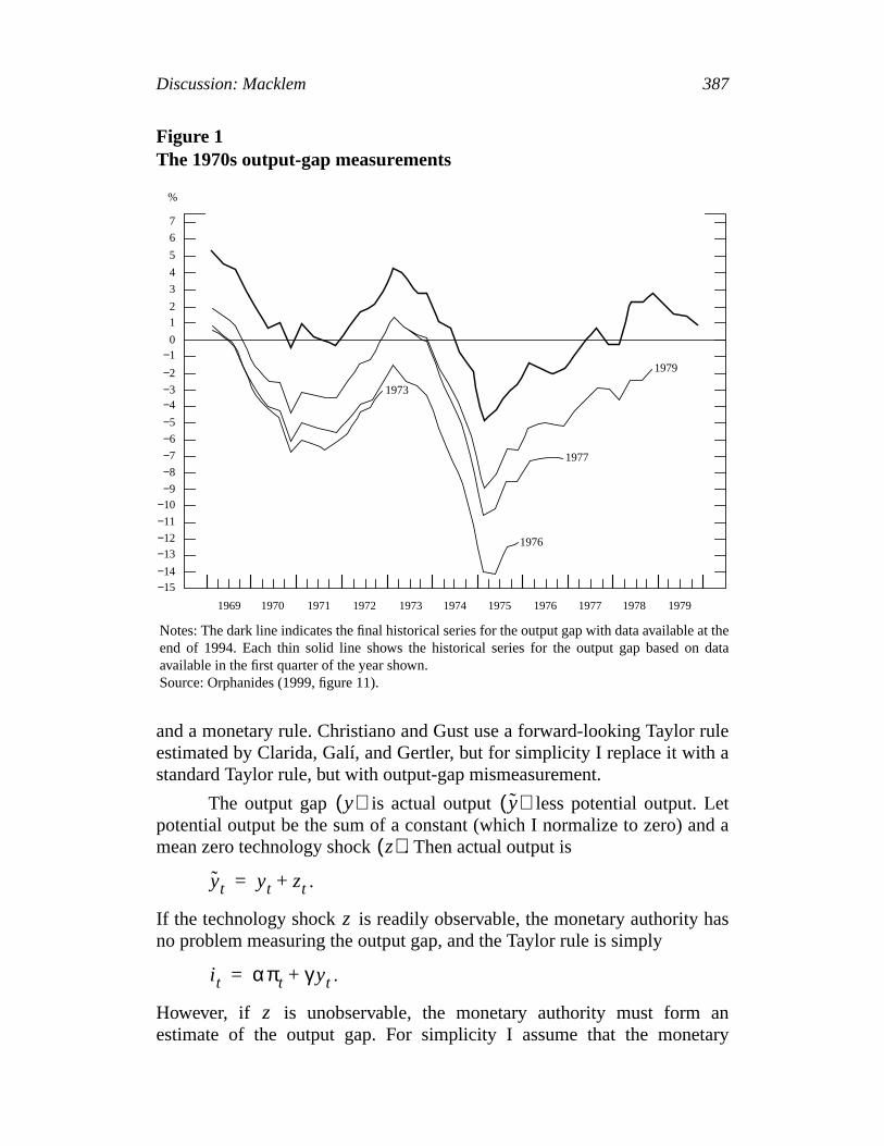
Discussion: Macklem 387
rulea
etd a
has
antary
Figure 1The 1970s output-gap measurements
7
6
5
4
3
21
0−1
−2
−3−4
−5
−6
−7
−8
−9−10
−11
−12−13
−14−15
1969 1970 1971 1972 1973 1974 1975 1976 1977 1978 1979
%
1979
1977
1973
1976
Notes: The dark line indicates the final historical series for the output gap with data available at theend of 1994. Each thin solid line shows the historical series for the output gap based on dataavailable in the first quarter of the year shown.Source: Orphanides (1999, figure 11).
and a monetary rule. Christiano and Gust use a forward-looking Taylorestimated by Clarida, Galí, and Gertler, but for simplicity I replace it withstandard Taylor rule, but with output-gap mismeasurement.
The output gap is actual output less potential output. Lpotential output be the sum of a constant (which I normalize to zero) anmean zero technology shock . Then actual output is
.
If the technology shock is readily observable, the monetary authorityno problem measuring the output gap, and the Taylor rule is simply
.
However, if is unobservable, the monetary authority must formestimate of the output gap. For simplicity I assume that the mone
y( ) y( )
z( )
yt yt zt+=
z
i t απt γ yt+=
z

388 Discussion: Macklem
realto be
oritynce
amers ,dard
amicsolidnt arehe
andeas-
ion.e seeandrest
ith athelemalreal
verrestct oftputvery
inse toas inatescess
st,ative
ust
authority does not learn about over the horizon that is relevant for theeffects of monetary disturbances, an assumption that does not appeargrossly at odds with experience (see Figure 1). The monetary auththerefore measures the gap by simply observing output (siunconditionally . The resulting Taylor rule istherefore
.
Figure 2 shows the dynamic response of this SP model to the snegative technology shock Christiano and Gust consider. The paramete
, and are set as they have them, and and are set to the stanTaylor values of 1.5 and 0.5. The dashed lines in the figure are the dynresponse in the standard SP model with no mismeasurement, and thelines are with mismeasurement. The consequences of mismeasuremesignificant. In particular, inflation jumps about twice as much in tsimulations with mismeasurement. Real interest rates also rise lessoutput falls less with mismeasurement, but the consequences of mismurement for these variables are small relative to those for inflatComparing the responses in Figure 2 to the experience of the 1970s, wthat the model with mismeasurement captures the sharp rise in inflationthe fall in output, but does not replicate the observed decline in real interates.
Figure 3 shows the dynamic responses to the same shock wmodified Taylor rule that shifts more weight onto the output gap, witheffect of making output-gap mismeasurement more of a prob(specifically and . Without mismeasurement the reinterest rate rises (as in Figure 2); however, with mismeasurement theinterest rate falls. This produces a very dramatic rise in inflation of o25 percentage points. The stimulative effects of the negative real interates produce a small positive output gap that offsets some of the impathe negative technology shock on output, but not all of the impact, so oufalls, getting us closer to the 1970s in the sense that inflation risessharply, and real interest rates and output both fall. However, asChristiano and Gust’s analysis, the output gap goes positive in responnegative real interest rates, and the reason is exactly the sameChristiano and Gust’s analysis. In the SP model, declining real interest rstimulate spending that, in this demand-driven model, produces exdemand for goods.
What can we learn from this exercise? Two things, I think. Firwhether the 1970s are interpreted as the by-product of an observed negtechnology shock and a destabilizing monetary or anunobserved negativetechnology shock with a stable rule, the SP model Christiano and G
z
E y( ) E y z–( ) y)= =
i t απt γ y+ απt γ yt zt+( )+= =
σβ κ α γ
α 1.1= γ 1.0)=

Discussion: Macklem 389
Figure 2Response to observed and unobserved negativetechnology shocks with a standard Taylor rule
0.5
0.0
−0.5
−1.0
−1.50 2 4 6 8 10 12 14
Z-shock
0 2 4 6 8 10 12 14
8
6
4
2
0
Inflation rate (%)(deviation from steady state)
8
6
4
2
00 2 4 6 8 10 12 140 2 4 6 8 10 12 14
0.5
0.0
−0.5
−1.0
−1.5
−2.0
Output(percentage deviation from steady state)
Interest rate (%)(deviation from steady state)
0.5
0.0
−0.5
−1.00 2 4 6 8 10 12 14
Output gap0.20
0.15
0.10
0.05
0.000 2 4 6 8 10 12 14
Real interest rate (%)(deviation from steady state)
Note: Solid lines, with error; dash lines, no error.
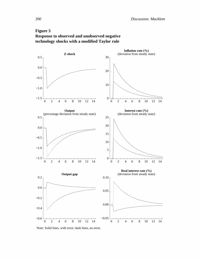
390 Discussion: Macklem
Figure 3Response to observed and unobserved negativetechnology shocks with a modified Taylor rule
0.5
0.0
−0.5
−1.0
−1.50 2 4 6 8 10 12 14
Z-shock
0 2 4 6 8 10 12 14
30
20
10
0
Inflation rate (%)(deviation from steady state)
25
20
15
10
00 2 4 6 8 10 12 140 2 4 6 8 10 12 14
0.5
0.0
−0.5
−1.0
−1.5
Output(percentage deviation from steady state)
Interest rate (%)(deviation from steady state)
0.2
0.0
−0.2
−0.60 2 4 6 8 10 12 14
Output gap0.10
0.05
0.00
−0.050 2 4 6 8 10 12 14
Real interest rate (%)(deviation from steady state)
5
−0.4
Note: Solid lines, with error; dash lines, no error.

Discussion: Macklem 391
ion,muchupplymayb ofwill
s toem totheiallyrious
eas-tput
ted,rule
ds)aker
thee,risen forto
apt istudyin
he
LP70s-utthisring.
consider has difficulty in simultaneously generating sharply higher inflatnegative real interest rates, and a negative output gap. The reason isthe same in both cases. This simple SP model has a very rudimentary sside, and what supply side it does have is weakened by sticky prices. Itwell be that an SP model with a richer supply side could do a better joexplaining the 1970s, but as long as sticky prices are active, demandtend to play a leading role in the short run.
I leave it to the experts to explore whether the LP model continueexplain the 1970s under the mismeasurement story, and I encourage thdo so. If Christiano and Gust find that the LP model does better thanSP model under both interpretations of the 1970s, this would substantstrengthen their conclusion that the lessons from LP models deserve seattention.
Second, the obvious message from the SP model with mismurement is that policy-makers should not put too much weight on the ougap if they are not very confident in its measurement.1 Figure 4demonstrates this point in a particularly forceful, if somewhat exaggerafashion. It compares the dynamic responses using a standard Taylor(i.e., and and an inflation-only rule (i.e., an
, both with mismeasurement. The inflation-only rule (solid linedoes result in slightly higher real interest rates and thus marginally weoutput. But these differences are second order when compared toimprovement realized on the inflation front. With the inflation-only rulinflation rises by only about 1/2 of a percentage point as compared to aof about 7 percentage points using the standard Taylor rule. The reasothis sharply different outcome is that the inflation-only rule is immunemismeasurement of the output gap.
Interestingly, the message from this SP model with output-guncertainty is very similar to a key result in LP models. In a paper thaclosely related to their conference paper, Christiano and Gust (1999) sthe performance of Taylor rules in LP models. They find that equilibriawhich expectations of inflation are self-fulfilling are eliminated when tTaylor rule respondsaggressivelyto inflation andvery little to output (e.g.,they find results in indeterminant solutions).
Perhaps the message for monetary policy-makers from bothmodels and SP models is that if they are to avoid the recurrence of 19style inflation, they should limit their ambitions with respect to outpstabilization and keep the focus on inflation. The robustness ofconclusion across radically different models is both striking and reassu
1. This idea is by no means original (see, for example, Smets 1998).
α 1.5= γ 0.5)= α 1.5=γ 0.0)=
γ 1.0=

392 Discussion: Macklem
Figure 4Response to unobserved negative technology shockswith inflation-only and standard Taylor rules
0.5
0.0
−0.5
−1.0
−1.50 2 4 6 8 10 12 14
Z-shock
0 2 4 6 8 10 12 14
Inflation rate (%)(deviation from steady state)
8
6
4
2
0 2 4 6 8 10 12 140 2 4 6 8 10 12 14
1
0
−1
−2
−3
Output(percentage deviation from steady state)
Interest rate (%)(deviation from steady state)
0.5
0.0
−0.5
−1.50 2 4 6 8 10 12 14
Output gap0.25
0.10
0.05
0.000 2 4 6 8 10 12 14
Real interest rate (%)(deviation from steady state)
0
−1.0
8
6
4
2
0
0.20
0.15
Note: Solid lines, inflation only; dash lines, standard Taylor.

Discussion: Macklem 393
ng
lity:
per
References
Chari, V.V., L.J. Christiano, and M. Eichenbaum. 1998. “Expectation Traps and Discretion.”Journalof Economic Theory 81 (2): 462–92.
Christiano, L.J. and C. Gust. 1999. “Taylor Rules in a Limited Participation Model.” NBER WorkiPaper No. 7017.
Clarida, R.H., J. Galí, and M. Gertler. 1998. “Monetary Policy Rules and Macroeconomic StabiEvidence and Some Theory.” NBER Working Paper No. 6442.
Orphanides, A. 1999. “The Quest for Prosperity without Inflation.” Board of Governors of theFederal Reserve System, Washington, D.C. Photocopy.
Smets, F. 1998. “Output Gap Uncertainty: Does it Matter for the Taylor Rule?” BIS Working PaNo. 60.

r ofe asthathigh
ingivateithern thenan
eyonshowtaryp.an
t oftwoleadcts
Christiano and Gust’s paper is concerned with explaining the behavioubase-money growth in the United States during the 1970s. They takgiven that the Fed was responsible for the great inflation witnessed indecade and that Fed policy-makers were very averse to the prospect ofinflation. Why, then, did the Fed do it?
Their hypothesis is that the Fed was reluctantly drawn into inflatessentially because this was what was expected of it. Given a jump in prsector expectations, the Fed perceived its choice as one of eaccommodating these expectations or risking a serious recession. GiveFed’s known proclivity for accommodation, private sector inflatioexpectations became a self-fulfilling prophesy. The Fed got caught in“expectations trap.”
Exactly why private sector inflation forecasts jumped the way thallegedly did is not explained; Christiano and Gust view the “expectatishock” as an exogenous impulse. What is explained, however, isparticular institutional arrangements that govern the conduct of monepolicy can give rise to the logical possibility of an expectations traMonetary policy in the 1970s is alleged to have operated in suchinstitutional setting. The authors formalize these ideas within the contexa computable dynamic general-equilibrium model and demonstrate howexogenous shocks—one to productivity and one to expectations—canto a 1970s-style stagflation. Their model’s ability to account for the fa
Discussion
David Andolfatto
394
* I would like to thank Lawrence Christiano, Ig Horstmann, David Laidler, and Ed Nosalfor a number of helpful conversations.

Discussion: Andolfatto 395
rpre-e by
itcant oftionive., theetter.
veryholds.
orheychthe
ible
ledmul-nt’shottioneyual
tedmmy
xpectanructFor
lends some credence to their argument. They also support their intetation of events by appealing to a number of selected statements madArthur Burns (Federal Reserve chairman, 1970–77).
Overall, I view their paper as an impressive piece of work;constitutes a wonderful example of how modern macroeconomic theorybe applied to important and difficult questions concerning the conducmonetary policy and the interpretation of monetary history. The explanaof events is original and the application of quantitative theory innovatEven if one is, as myself, not persuaded by the argument offered herepaper lays down a standard and invites competing explanations to do bIn all these senses their paper constitutes a valuable contribution.
The Expectations Trap
The basic idea of an expectations trap can be presented in terms of asimple game. Suppose that there are two players, the Fed and houseThe Fed has two possible actions: It can either choose a low inflationa high inflation . Likewise, households have two possible actions: Tcan expect either low inflation or high inflation. The utility payoff to eaplayer depends not only on its own action, but also on the actions ofother player. With two players and two actions, there are four posspayoff configurations (see Figure 1).
The payoff structure displayed in Figure 1 gives rise to what is cala coordination game. Players are imagined to make their choices sitaneously (they cannot condition their behaviour on their opponebehaviour). So two pure-strategy Nash equilibria exist for this one-sgame: one in which households and the Fed coordinate on a low-inflaequilibrium (each receiving a payoff equal to “1”), and one in which thcoordinate on a high-inflation equilibrium (each receiving a payoff eqto “0”).1
A question naturally arises here as to which of the two coordinaoutcomes is more likely to transpire; this is the question of equilibriuselection posed by game theorists. Unfortunately, to the best of
1. There is also a mixed-strategy equilibrium in which both the Fed and households ethe low-inflation regime with probability (1/3). In this case a “coordination failure” coccur with positive probability. By suitably modifying the game, one can also constcorrelated (sunspot) equilibria that eliminate the possibility of coordination failure.simplicity I will concentrate solely on pure strategies.
ΠLΠH

396 Discussion: Andolfatto
thetuteson)
willo doatethisusteat
old
, inholdseousmto
iateplinefittingthebut
nomy
ationothersnary
nousation
ock
Figure 1The game
Households
TheFed
1 −1
1 −1
−1 0−1 0
ΠL ΠH
ΠL
ΠH
knowledge there is still no good answer to this question.2 So we see herethat the prevailing institutional structure (the rules and structure ofgame) gives rise to a fundamental indeterminacy: Either outcome constia logical possibility. In the game, if households expect (for whatever reasthat inflation is to be high, then the Fed, anticipating this expectation,have an irresistible incentive to accommodate these expectations. Totherwise would invite coordination failure. But if the Fed plans to genera high inflation, then households are perfectly rational in expecting it. Inway, high expectations of inflation can be self-fulfilling. Christiano and Gexploit exactly this type of indeterminacy in their explanation of the grinflation.
In applying their theory they invoke the assumption that househinflation expectations are subject to exogenous shocks.3 By specifying sucha process the theorist is in effect selecting an equilibrium. For examplethe context of the game, suppose that I simply assume that housechoose (or that households choose on the basis of some extraninformation).4 Conditional on this assumed behaviour, the only equilibriuis the low-inflation outcome. It would appear that the theorist is now freechoose any desired outcome simply by specifying the approprexogenous process for inflation expectations. One way to impose discion the exogenous expectations process is to estimate its parameters bythe model to the data. Obviously this exercise is not going to answerquestion of why inflation expectations bounce around the way they do,the estimated model can be used to answer the question of why the eco
2. There are some axiomatic approaches to selecting among equilibria for coordinproblems. Some are simple (choose the Pareto dominant one, if there is one), whileare more complicated (see Myerson 1991). The literature on learning and on evolutiogames also attempts to address this issue.3. Alternatively, one might hypothesize that it is Fed behaviour that is subject to exogeshocks. Technically, I do not believe anything would change aside from the interpretof events.4. Technically, by allowing individuals to condition their strategies on some external shor information, I have implicitly modified the one-shot game described above.
ΠL ΠL

Discussion: Andolfatto 397
d theess
s forcycle
thewas
Theonse thef theome
ntsanmo-
edthatndbe
relythe
amedo
ndhyinto, thehe
ightditionenousture
ofting
theer;
behaves the way it does given that inflation expectations bounce arounway they do. Methodologically this is no different than, say, a real busincycle theorist estimating the parameters of an exogenous procestechnological change and then offering an explanation of the businessconditional on this estimated exogenous process.
The exact procedure Christiano and Gust employ in explaininggreat inflation is to assume that over the relevant sample period thereone exogenous upward shift in inflation expectationsand that this shiftoccurred coincidently in the period of an adverse technology shock. (model provides absolutely no theoretical rationale for why expectatimove the way they do in response to the supply shock, however plausiblargument may sound on other grounds.) The quantitative magnitude oshift in expectations seems to have been calibrated to match sunspecified price-level response in the period of the technology shock.
The model provides an intriguing interpretation of economic evein the early 1970s. The choice of a modelling framework that featuresequilibrium indeterminacy, exogenous expectations shocks, and accomdative monetary policy seems to fit well with a number of recordstatements made by policy-makers in that era. For example, we knowBurns did not view monetary policy as the ultimate driving force behiinflation; at the same time, he recognized that inflation could notsustained without money growth. In his view, monetary policy was seveconstrained by a host of political and economic factors that compelledmonetary authority to behave the way it did (see Hetzel 1998). The gdescribed above reflects this point of view; the monetary authority canlittle aside from adopting the “accommodative” Taylor rule Christiano aGust employ in their quantitative investigation. This view also explains wBurns fought so hard to have a system of wage and price controls putplace. To the extent that wage and price controls can be made crediblepublic would be compelled to form low expectations of inflation, and tmonetary authority could therefore avoid being pushed into inflating.
Criticism
In any theory or explanation a theorist must take a stand on what mappropriately be treated as exogenous for the purpose at hand. The train monetary economics has been to hypothesize the existence of exogshocks to monetary policy (with expectations accommodating the strucof monetary policy). Christiano and Gust hypothesize the existenceexogenous shocks to expectations (with monetary policy accommodathe structure of expectations). I have no problem with exploringimplications of reversing the direction of causality in such a mann

398 Discussion: Andolfatto
eemriable
ionple,tiongly,ationthensnceally
ctualthest isfromowrate, ing a4,t. Intingionratehis
forilityreaseney
eadsthatandthe
hinkta isather
howsation.
however, in emphasizing the role of an exogenous variable, it would sdesirable for the researcher to first take some measurements of the vain question (e.g., see Prescott 1986).
There are, in fact, many independent measures of inflatexpectations for the time period Christiano and Gust study. For examThomas (1999) reviews three popular survey measures of inflaexpectations for the United States beginning in 1960. Interestinregardless of how they are measured, year-to-year forecasts of inflsince 1960 consistently display an “inertial” tendency. In particular, overperiod of generally rising inflation (1965–80), inflation expectatiotypically lagged (underestimated) the actual inflation rate. Likewise, sithe disinflation of the early 1980s, inflation expectations have generlagged (overestimated) the actual inflation rate.5
To give the reader a feel for these data, Figure 2 reproduces the aGDP deflator inflation and the previous year’s forecast of inflation inUnited States over the 1969–94 sample period. The inflation forecabased on a survey of professional forecasters; the data are takenFigure 6.9 in De Long (1997). A striking feature of these data is hexpectations of inflation consistently underestimated the actual inflationthrough most of the 1970s; however, what is even more striking is howvirtually each and every year, private forecasters were expectindisinflation. Consider, for example, the inflation “takeoff” of 1973 and 197when inflation rose from 4.5 per cent to 6.5 per cent and 8.8 per cenDecember 1972, with inflation at 4.5 per cent, forecasters were predicfor 1973 an inflation rate of 3.9 per cent. In December 1973, with inflatrunning at 6.5 per cent, forecasters were predicting for 1974 an inflationof 5.4 per cent. My reading of De Long (1997) is that policy-makers of tera generally shared in these “optimistic” forecasts.
So my question to Christiano and Gust is: Where is the evidencethis alleged expectations shock? In my view their argument’s plausibrequires evidence of a sharp increase in inflation expectations, an incthat either precedes or is at least coincident with an increase in mogrowth. In the data, however, money growth leads inflation and hence linflation expectations by even a greater extent. One could try to arguethe sharp rise in base-money creation beginning in 1970 (see ChristianoGust’s Figure 2) was engineered by the Fed in order to accommodaterise in inflation expectations expected to occur around 1974–75, but I tthat this is stretching things. A more plausible interpretation of these dathat inflation expectations are not subject to unaccountable shocks but r
5. Dotsey and DeVaro (1995) also find that their measure of inflation expectations sa persistent tendency to overestimate the actual inflation rate during the 1980s disinfl

Discussion: Andolfatto 399
uth
ee.ngs)ssuee
tionn.)
t intlays
ling
ethe
thisrightto
nge
Figure 2Inflation and expected inflation in the United States, 1969–94
InflationExpected inflation
Wage and price controls(August 1971–April 1974)
12
10
8
6
4
2
70 72 74 76 78 80 82 84 86 88 90 92 94
%
are fully endogenous, responding optimally in an adaptive manner (M1960) to new information as it becomes available.6
An Alternative Hypothesis
When I view the historical evidence over the last century, this is what I sThere were three (possibly four, depending on how you measure thiinflationary episodes: 1916–20, 1940–46, and 1965–80. (Here I take iwith Christiano and Gust’s dating of the “inflation takeoff”; to my eye thtakeoff seems to have occurred in 1965, with the 1969–70 disinflarepresenting a cyclical deviation from the general trend of rising inflatioEach episode is characterized by three things: (1) a major shifgovernment expenditure and/or outlays, (2) pressure to finance these ouwith paper (new debt or new money), and (3) a breakdown of a prevaiinternational monetary institution.
In the first great inflation we had the First World War and thbreakdown of the gold standard. In the second great inflation we hadSecond World War and a breakdown in the gold standard (admittedlygold standard was abandoned in the 1930s, so the timing is not quitehere). In the third great inflation there was the Vietnam War in additionthe “war on poverty” and a breakdown of the Bretton Woods fixed excha
6. See, for example, Andolfatto and Gomme (2000).

400 Discussion: Andolfatto
the
usedt belic’sionalty offor
tible
0s.y asentsncetheente onney
it isenuetates
, theply;ited.S.
eir, thede it
pertton
ard.f angerngeforndsot to
on
rate system, which formally ended in 1971 when Nixon abandoneddollar’s peg to gold.
The appropriate exogenous event would seem to be whatever cathe major shift in government expenditure. In the case of a war, this mighmodelled as an exogenous (and transitory) shift in the general pubpreferences for output that is to be consumed in the enforcement of natproperty rights. People know what comes with war: an increased scarcigoods for private use, mounting fiscal deficits (nominally denominated,that matter), a weakening of peacetime institutions, and an irresistemptation to resort to new money creation.
The Vietnam War was peaking in the late 1960s and early 197Military expenditures were placing great strain on the American economreal resources were being consumed in unproductive ways. PresidJohnson and Nixon were naturally reluctant to raise taxes in order to finathe outlays required to meet the growing demands of the war effort andgrowing demands for social spending. The arithmetic of the governmbudget constraint implies that there must have been a growing reliancother forms of finance, in particular the issuance of new paper (new moand debt) and/or the default on existing paper (monetizing the debt).7
Seigniorage revenue is often dismissed as “small potatoes,” butlikely that reported statistics greatly understate seigniorage as a revsource under a system of fixed exchange rates. When the United Srapidly increased the rate of base-money creation beginning in 1965relevant “tax base” under Bretton Woods was the world money supforeigners were conceivably contributing significant resources to the UnStates as inflation around the world soared owing to the proliferation of Udollars. As foreign countries struggled to maintain control over thdomestic monetary policies through a series of currency re-evaluationsfixed exchange rate system began to come apart. The inflation also maincreasingly painful to maintain the value of American currency at $35ounce of gold; in 1971, the gold standard was abandoned and BreWoods ceased to exist.
It was the fiscal authority (Nixon) that abandoned the gold standWhy? One argument is that by doing so, the Fed (Burns) was relieved oimportant constraint on the rate of money creation (it was no loncompelled to maintain the nominal anchor to gold). This institutional chaimplied that the Fed was more susceptible to political pressureaccommodative behaviour. This political pressure took the form of demafor more spending (on both Vietnam and the Great Society), demands n
7. The unanticipated inflation of the early 1970s implied a significant implicit defaultoutstanding nominal debt (see Auerbach and Kotlikoff 1995, 300).

Discussion: Andolfatto 401
70sissuetion?dateation.Forgust
ich
reock.rgue.
ar
inedicalte. Ine of
increase taxes (for fear of crippling consumer demand in the weak 19economy), and demands not to increase the rate of government debt(bad for business psychology). What was the Fed to do in such a situaOne answer is that the Fed could do what it did: reluctantly accommothese demands by increasing (or not decreasing) the rate of money creThe narrative I provide here is not inconsistent with Burns’s own views.example, according to Burns’s testimony to the U.S. Congress in Au1974 (Hetzel 1998, 35):
The current inflationary problem emerged in the middle 1960swhen our government was pursuing a dangerously expansivefiscal policy. Massive tax reductions occurred in 1964 and thefirst half of 1965, and they were immediately followed by anexplosion of Federal spending. . . . Ourunderlying inflationaryproblem, I believe, stems in very large part from loose fiscalpolicies.
In 1979 he gave a speech called “The Anguish of Central Banking” in whhe stated (Hetzel 1998, 34):
Once it was established that the key function of governmentwas to solve problems and relieve hardships—not only forsociety at large but also for troubled industries, regions,occupations, or social groups—a great and growing body ofproblems and hardships became candidates for governmentsolution. . . . Their [government programs’] cumulative effect. . . was to impart a strong inflationary bias to the Americaneconomy. . . . My conclusion that it is illusory to expectcentral banks to put an end to the inflation that now afflicts theindustrial economies does not mean that central banks areincapable of stabilizing actions; it simply means that theirpractical capacity for curbing inflation that is driven bypolitical forces is very limited.
According to my interpretation, while general expectations weimportant, they simply reflected the nature of a fundamental fiscal shExpectations were not an indeterminate entity, as Christiano and Gust aIn fact, I will go so far as to argue that inflation expectations were likelyvery important factor in curtailing the rate of inflation. Imagine, foexample, what might have happened if Americans (for some unexplareason) always expected zero inflation. I conjecture that the politdemands for new money would have been even easier to accommodacontrast, the Christiano and Gust model would suggest the absencinflation.

402 Discussion: Andolfatto
s totwo
illipsetaryng iniblyenseer
ogyan(as
ons,
hell anthelicyto
ismthe
ank
go
Conclusion
Christiano and Gust’s interpretation of the most recent great inflation itreat the general rise in inflation over the late 1960s and early 1970s asseparate episodes. The first episode is explained in terms of their Phcurve hypothesis, the second by an expectations trap. The monauthority at that time is described as being weak in the sense of operatian institutional environment that encouraged it to accommodate posswhimsical private sector expectations (as opposed to being weak in the sof readily capitulating to the demands of the fiscal authority or othpolitical forces). They hypothesize the arrival of an adverse technolshock that temporarily increased the inflation rate and the arrival ofexpectations shock that propagated the higher inflation forward in timethe monetary authority accommodated the higher inflation expectatithereby making them self-fulfilling).
As usual, many different interpretations of history are possible. Tbest way in which to understand the causes of the 1970s inflation is stiopen question. However, it is encouraging to note that whileexplanations offered above may differ, they share a common poimplication. In particular, one way to prevent inflationary outbursts isendow the monetary authority with a credible commitment mechan(possibly through legislation) that prevents it from ever capitulating toincessant demands for new money.
References
Andolfatto, D. and P. Gomme. 2000. “Monetary Policy Regimes and Beliefs.” Federal Reserve Bof Cleveland. Photocopy.
Auerbach, A.J. and L.J. Kotlikoff. 1995.Macroeconomics: An Integrated Approach. Cincinnati:International Thomson.
De Long, J.B. 1997. “America’s Peacetime Inflation: The 1970s.” InReducing Inflation: Motivationand Strategy, edited by C.D. Romer and D.H. Romer, 247–80. Chicago: University of ChicaPress.
Dotsey, M. and J.L. DeVaro. 1995. “Was the Disinflation of the Early 1980s Anticipated?”FederalReserve Bank of Richmond Economic Quarterly81 (4): 41–59.
Hetzel, R.L. 1998. “Arthur Burns and Inflation.”Federal Reserve Bank of Richmond EconomicQuarterly84 (1): 21–44.
Muth, J.F. 1960. “Optimal Properties of Exponentially Weighted Forecasts.”Journal of theAmerican Statistical Association 55 (290): 299–306.
Myerson, R.B. 1991.Game Theory: Analysis of Conflict. Cambridge, Mass.: Harvard UniversityPress.
Prescott, E.C. 1986. “Theory Ahead of Business Cycle Measurement.”Federal Reserve Bank ofMinneapolis Quarterly Review 10 (4): 9–22.
Thomas, L.B., Jr. 1999. “Survey Measures of Expected U.S. Inflation.” Journal of EconomicPerspectives 13 (4): 125–44.

themicns of
s oftual
vidighnd
icand
gain.ond ationcalaybeicthental
f thenotthat
General Discussion
David Laidler commented that the study of Fed behaviour and motives in1970s should take into account the state of informed opinion, or econoknowledge, attained in those years. This state was such that expectatioinflation and, in general, forward-looking behaviour, as well as the levelmoney stocks, were thought to have little bearing in determining the aclevel of inflation at a point in time.
Jean-Pierre Aubry agreed with Laidler and also agreed with DaAndolfatto’s comment that inflation expectations were not relatively hand leading indicators of ever higher inflation, but were relatively low alagging indicators of inflation during the seventies.
Marvin Goodfriend wondered how much the present economsystem is susceptible to such positive shocks in inflation expectationswhether there is a danger of such an inflation spiral appearing once aHe also agreed with Andolfatto’s opinion that it didn’t seem that inflatiexpectations were relatively high in the seventies. Goodfriend offerepossible rationalization of the Fed’s incentive to accommodate inflaexpectations and not strongly intervene to contain inflation: Politipressures on the Fed’s independence were growing in the sixties, so mit could not afford to disregard contractionary policy’s effect on economactivity. The undermining of the Bretton Woods system also meant thatFed was left with neither a clear nominal anchor nor a clear fundameobjective for most of that decade.
Charles Freedman asserted that economists deserved some oresponsibility for the increase in inflation in the seventies. Many didrecognize that high inflation had substantial costs, or they concluded
403
* Prepared by Kevin Moran.

404 General Discussion
illips
ntthel.
ubtthe
es,iontry
s intory
these costs were small compared to the benefits of moving up the Phcurve (Harberger triangles were small and Okun’s gaps large).
Christopher Gust commented that he liked Tiff Macklem’s commeand the simulation included in it and would have liked to have seenresults of Macklem’s simulation done with the limited-participation mode
Lawrence Christiano thanked the commenters. He put into doAndolfatto’s assertion that high fiscal pressure had most often beenunderlying cause of (eventual) high inflation by pointing to the eightiwhen the American fiscal position continuously deteriorated while inflatwas brought into control. He also welcomed Andolfatto’s suggestion toto identify and quantify the exogenous shocks to inflation expectationtheir model. Christiano also mentioned that their model and the sderived from it could also be interpreted in a monetarist framework.