The equilibrium of rubble-pile satellites: The

Darwin and Roche ellipsoids for

gravitationally held granular aggregates

Ishan Sharma

Department of Mechanical Engineering, IIT Kanpur, Kanpur 208016, India.

Abstract

Many new small moons of the giant planets have been discovered recently. In paral-lel, satellites of several asteroids, e.g., Ida, have been found. Strikingly, a majority ofthese new-found planetary moons are estimated to have very low densities, which,along with their hypothesized accretionary origins, suggests a rubble internal struc-ture. This, coupled to the fact that many asteroids are also thought to be particleaggregates held together principally by self-gravity, motivates the present investiga-tion into the possible ellipsoidal shapes that a rubble-pile satellite may achieve asit orbits an aspherical primary. Conversely, knowledge of the shape will constrainthe granular aggregate’s orbit - the closer it gets to a primary, both primary’s tidaleffect and the satellite’s spin are greater. We will assume that the primary bodyis sufficiently massive so as not to be influenced by the satellite. However, we willincorporate the primary’s possible ellipsoidal shape, e.g., flattening at its poles inthe case of a planet, and the proloidal shape of asteroids. In this, the present inves-tigation is an extension of the first classical Darwin problem to granular aggregates.

General equations defining an ellipsoidal rubble pile’s equilibrium about an el-lipsoidal primary are developed. They are then utilized to scrutinize the possiblegranular nature of small inner moons of the giant planets. It is found that mostsatellites satisfy constraints necessary to exist as equilibrated granular aggregates.Objects like Naiad, Metis and Adrastea appear to violate these limits, but in do-ing so, provide clues to their internal density and/or structure. We also recoverthe Roche limit for a granular satellite of a spherical primary, and employ it tostudy the Martian satellites, Phobos and Deimos, as well as to make contact withearlier work of Davidsson (Icarus 149 [2001], 375). The satellite’s interior will bemodeled as a rigid-plastic, cohesion-less material with a Drucker-Prager yield crite-rion. This rheology is a reasonable first model for rubble piles. We will employ anapproximate volume-averaging procedure that is based on the classical method ofmoments, and is an extension of the virial method (S. Chandrasekhar, EllipsoidalFigures of Equilibrium, Yale U. Press [1969]) to granular solid bodies.

Preprint submitted to Elsevier Science 18 November 2008

1 Introduction

Roche (1847) first considered the problem of finding the equilibrium shapeof a fluid satellite of a spherical planet, identifying ellipsoidal equilibriumshapes now known as the Roche ellipsoids. Later, Darwin (1906) introduced anon-trivial generalization of the Roche problem: the characterization of equi-librium shapes of two tidally interacting fluid bodies that rotate about eachother on circular orbits. Chandrasekhar (1969) showed that, at least in thecase of fluids, there are only two possible scenarios in which such ellipsoidalequilibrium shapes may be found. The first is when the aspherical primary ismassive enough to warrant neglecting the tidal effects due to the satellite. Inthe other case, both objects are congruent, i.e., with the same shape, massand in a symmetric orientation. Indeed, Darwin (1906) himself had empha-sized this dichotomy. We will refer to this natural classification as the firstand second Darwin problems, whose solution, for an inviscid fluid, yields theDarwin sequence of ellipsoids (Chandrasekhar 1969).

Recently, several small inner moons of the giant planets have been discovered.Their estimated low densities, often lower than or comparable to water’s, sug-gests that these objects may be either granular aggregates, or highly porouscellular “honeycomb”-like structures. While the former, in the absence of co-hesion, has no tensile strength and is held together only by its own gravity, thelatter is able to withstand a certain amount of tension. It is, however, believedthat these newly uncovered satellites may have formed via an accretionaryprocess either from ring particles, as in the case of Saturn’s moons (Porcoet al. 2007), or from the debris left over from some past catastrophic event,e.g., Neptune’s capture of Triton (Banfield and Murray 1992). There is thusa need to generalize the first of the two classical Darwin problems introducedabove to rubble-pile satellites of oblate planets. In fact, the finding of asteroidalsatellites, many of which are suspected particle aggregates, strongly suggeststhe need to consider also elongated triaxial primaries. The general scenario isdisplayed in Fig. 1.

Rubble piles, while much weaker than coherent structures, are able to sustainshear stresses due to internal friction. This allows a range of stable satelliteshapes to be possible at a given planetary distance. Conversely, for a givenshape, the satellite’s orbits on which it may persist in equilibrium are not nec-essarily unique. In the sequel, we will obtain general equations that describethe equilibrium landscape of a triaxial-ellipsoidal, tidally-locked, rubble-pilesatellite on a circular orbit around a triaxial-ellipsoidal primary. The formula-tion will then be specialized to investigate the moons of the giant planets. InSec. 5, the Roche limit for a granular aggregate, i.e., the critical distance at

Email address: ishans@iitk.ac.in (Ishan Sharma).

2

Primary

Satellite

e1’

e2

e2’

e3’

e1

e3

R

PP

S

Orbital plane

eR

Fig. 1. The general configuration of an ellipsoidal satellite of an ellipsoidal primary.The unit vector eR locates the satellite with respect to the primary’s center.

which a rubble-pile satellite may orbit a spherical planet, will also be obtainedas a special case and will then be employed to study the two satellites of Mars.Recently, Holsapple and Michel (2006, 2008) have considered the Roche limitfor solid bodies, employing the static version of Signorini’s theory of stressmeans (Truesdell and Toupin 1960, p. 574). We compare briefly with theirresults in Sec. 5.2.

We will employ a volume-averaging procedure that is really a generalizationof Chandrasekhar’s (1969) virial method to the statics, and dynamics, of solidobjects. Previously, this volume-averaging procedure has been employed toinvestigate tidal disruption during planetary flybys (Sharma 2004, Sharma etal. 2006), equilibrium shapes and dynamical passage into them for asteroids inpure spin (Sharma et al. 2005a, 2005b, 2008), and the Roche limit for rubblepiles (Sharma et al. 2005b, Burns et al. 2007). A good match with availablecomputational and analytical results was achieved. In fact, in the case of rubblepiles in pure spin, the equilibrium landscape obtained from volume-averagingmatched perfectly Holsapple’s (2001) exact results that were based on rigorouslimit analysis (Chen and Han 1988) often employed in rigid-plasticity.

We develop the governing equations next.

2 Volume-averaging

In this section, we present the main equations obtained from an application ofthe volume-averaging procedure. More details about derivations may be foundin Chandrasekhar (1969), Sharma et al. (2006), or Sharma et al. (2008).

3

In case of a tidally interacting satellite, there are principal-axes coordinate sys-tems associated with both the satellite and the primary. No particular systemis better suited to evaluate all quantities that will appear below. In addition,many different relative orientations of the primary and the satellite are possi-ble. Thus, it is advantageous to follow a coordinate-independent tensor-basedapproach. We will develop general equations, applicable to all primary-satelliteconfigurations, as far as possible, and only specialize to a particular primary-satellite configuration at the very end. We offer a very short primer on tensorsand operations with them in Appendix A. More information may be obtainedfrom Knowles (1998). The reader should also refer to Appendix A for notationsfollowed in this paper.

We now proceed to the governing equations.

2.1 Governing equations

We consider a finite-sized satellite in motion about a primary also of finitespatial extent. Much work has been done on the dynamical problem of relativeequilibria in the two finite rigid-body problem, and we refer the interestedreader to Kinoshita (1972), and more recently to Scheeres (2006). Indeed, thetwo finite rigid-body problem will be relevant when extending the present workto the equilibrium shapes in a binary system consisting of comparable masses,i.e., the second Darwin problem introduced in Sec. 1. In this paper, we focuson the first Darwin problem, wherein the primary is much more massive thanthe satellite. Thus, we neglect the motion of the primary’s center of mass. Wealso make the further assumption that the satellite moves around the primaryat a much faster rate than the primary around the Sun.

The stress σ inside a deformable body, such as a satellite, may be obtainedby solving the Navier equation (see, e.g., Fung 1965)

∇ · σ + ρb = ρ(x + R

), (1)

where ρ is the density, b the body force and x the location of a material pointwith respect to the satellite’s center of mass, and R locates the satellite’s mov-ing mass center with respect to the primary’s fixed center of mass (see Fig. 1).To solve the above partial differential equation, one must provide appropriateboundary conditions, and compatibility equations that incorporate the mate-rial’s constitutive behavior. Note that, within the approximations introducedin the preceding paragraph, x + R is the total acceleration of a material pointand x is the acceleration relative to the satellite’s mass center. The body forceincludes in our case the tidal effects of the primary on the satellite, and ofthe satellite’s internal gravity on itself. Except in the simplest of geometries,loading conditions, rheologies and small deformations, solving for the exact

4

stresses is often analytically intractable, and even computationally very in-volved. Considering the intricate constitutive nature of planetary bodies, theutility of undertaking such an exercise is also moot. Instead we follow anapproximate method here.

Volume-averaging begins by making systematic approximations to the body’sactual time-varying deformation field in terms of a finite number of only tem-porally dependent variables. Equations governing these variables are then ob-tained by taking an appropriate order moment of the linear momentum bal-ance equation (1) above. For example, the first moment, and the one utilizedin this work, is obtained by integrating the tensor product (A.2) of each quan-tity in (1) with the position vector x over the body’s volume V . This has theadvantage of converting the governing coupled non-linear partial differentialequations into a set of ordinary differential equations, easily integrated by aRunge-Kutta time-marching algorithm. The disadvantage is that our solutionsare valid on a global, rather than local, scale. The volume-averaging procedureis reminiscent of the Galerkin projection frequently employed in finite elementanalysis (e.g., Belytschko et al. 2000), and, in fact, an exact equivalence maybe demonstrated.

Here we consider the simplest non-trivial such kinematic assumption suitableto the problem at hand; a deformation that is homogeneous when viewed in anon-rotating coordinate system with its origin at the ellipsoidal satellite’s masscenter. We assume that the ellipsoidal satellite is homogeneous, so that its massand geometric centers coincide. Physically, this kinematic assumption enforcesthe condition that, in this coordinate system that orbits the primary alongwith the satellite, but does not rotate with the latter, an initially ellipsoidalshape deforms only into another ellipsoid. As noted earlier (Sharma et al.2008), homogeneous kinematics were shown to yield physically meaningfulresults in the case of spinning fluid masses by Chandrasekhar (1969). Furthermotivation is provided by the fact that spinning elastic ellipsoids, and alsotidally-stressed elastic ellipsoids, deform into ellipsoids (Love 1946, Murrayand Dermott 1999).

With the above kinematic assumption, the original position x0 of a mass pointwith respect to the satellite’s center of mass may now be related to its futurelocation x by

x = F · x0, (2)

in terms of the deformation gradient tensor F that depends only on time, andnot on the spatial coordinates. Thus, F incorporates the nine independenttemporal variables that we assume approximate the ellipsoid’s actual defor-mation. These variables roughly correspond to three stretches, three shearsand three rotations. For a rigid body, F is a rotation tensor. Rather thandeveloping equations for the components of F , as Sharma et al. (2006, 2008)

5

did, we first introduce the velocity gradient

L = F · F−1, (3)

so that the kinematic law (2) may be replaced by its equivalent incrementalform

x = L · x. (4)

Like F , L is also independent of x, depending only on time.

As indicated above, a sufficient number of equations for the components ofL are obtained by taking the first moment of (1), invoking the divergencetheorem to transform volume integrals, employing (3) to represent the veloc-ities x and accelerations x in terms of the position vector x and L, and finallyassuming a traction-free (force-free) surface. The resulting volume-averagedevolution equation for L is(

L + L2)· I = M T − σV, (5)

where σ is now the average stress (1/V )∫V σdV ,

I =∫Vρx⊗ xdV (6)

is the inertia tensor, and

M =∫V

x⊗ ρbdV (7)

is the moment tensor due to the body forces b. In the development above,the term

∫V x ⊗ R ρdV =

∫V x ρdV ⊗ R vanished because the satellite’s center

of mass is at x = 0. We note that under the assumption of homogeneouskinematics, the deformation and velocity gradients are constant throughoutthe body. Therefore the stresses too are independent of x, as they typicallydepend only on F and L. Consequently, the average stress σ equals the actualstress σ, and we subsequently drop the overbar on σ.

The inertia tensor’s evolution may be followed by first differentiating (6) whileconserving mass, and then invoking (4) and (6) to obtain

I = L · I + (I · L)T . (8)

Equations (3), (5) and (8) govern the motion of a homogeneously deformingellipsoid under the action of only the body forces b, once a constitutive lawrelating the stress σ to the body’s deformation is specified.

In general, the velocity gradient incorporates both the strain (or stretching)rate and the spin rate. The latter rate measures the local angular velocity ina deformable medium, and is usually distinct from the rotation rate of thebody’s principal axes. When the object is rigid, the strain rate vanishes and

6

the local spin rate coincides with the principal axes’ rotation rate. Thus in (5)we set L = W , the anti-symmetric tensor associated with the rigid body’sangular velocity (see (A.9)), to obtain(

W + W 2)· I = M T − σV. (9)

The three Euler equations (Greenwood 1988) governing a rigid body’s dynam-ics are recovered from the nine equations of (9) by taking its anti-symmetricpart, and noting that σ is symmetric. The remaining six equations yield theexact average stress inside the rigid body. Note that while it is impossible todefine a point-wise stress field in a rigid body, an average stress is well-definedand exactly obtainable, as is done above.

In the present analysis, we are concerned with tidally-locked equilibrium con-figurations of an ellipsoidal satellite on a circular orbit. Thus, the spin tensorW associated with the satellite’s rotation rate equals the satellite’s fixed or-bital angular velocity. A constant W is achieved when the torque given bythe anti-symmetric part of M vanishes, and the object spins about an axis ofprincipal inertia. Under these conditions, W and I commute and W 2 · I issymmetric. Setting W to zero in (9), and rewriting slightly, we find

σ =1

V

(M T −W 2 · I

), (10)

which is a volume-averaged balance between “centrifugal” stresses due to thesatellite’s rotation, stresses due to the body force as given by the body forcemoment tensor M , and the satellite’s internal strength. The above balance,along with a suitable failure law, will help put constraints on a satellite’sequilibrium shapes for a given spin and orbit size, as we illustrate below. Weemphasize that the above equation is valid for all ellipsoidal satellites andprimaries, with the only requirement being that the former be tidally lockedand on circular orbit about the latter. To address satellites that are not tidallylocked and/or on elliptic orbits, we will have to retain the term W in the aboveequation.

To obtain σ from (10), we require both M and W . Because we considertidally-locked satellites, W will be obtained from the satellite’s orbital motionin Sec. 2.4. We first calculate the body-force moment tensor M . Recall thatin our case the body force is due both to the satellite’s internal gravity andalso the tidal stresses introduced by the primary. Thus, we may write

M = M G + M Q, (11)

where M G is the moment tensor due to internal gravity, and M Q, the quadrupolemoment tensor, is the moment tensor due to tidal influence of the primary.The expressions developed in the following two subsections are applicable toall mutually interacting triaxial-ellipsoidal objects on possibly elliptical orbits.

7

A cautionary comment is in order here. Consider finding at a point withinthe satellite the total body force per unit mass due to both the finite-sizedsatellite and the primary. This body force at this point may be derived, aswe do, by adding to the internal gravity force of the satellite, the externalgravitational attraction of the primary. It may also be obtained by takingthe gradient of the total gravitational potential at that point of each body.The total gravitational potential at a satellite’s internal point is the sum ofthe satellite’s internal potential and the primary’s external potential. It isimportant to note that we are not attempting to find the mutual potentialof two finite-sized objects. This latter potential has been computed by manyauthors, see, e.g., Werner and Scheeres 2005; Ashenberg 2005, and is of interestwhen calculating the total energy of the system, which, however, is not theaim here.

2.2 Gravitational moment tensor

M G was derived in Sharma et al. (2006), and is

M G = −2πρGI ·A, (12)

where G is the gravitational constant and the gravitational shape tensor Adescribes the influence of the satellite’s ellipsoidal shape on its internal gravity(Chandrasekhar 1969; Sharma et al. 2006). The symmetric tensor A dependsonly on the axes ratios α = a2/a1 and β = a3/a1, and is completely knownfor any given ellipsoidal satellite. Moreover, like I , it is diagonalized in thesatellite’s principal-axes coordinate system. Thus, I and A commute. Relevantformulae for the components of A for general ellipsoidal shapes are available(Sharma et al. 2008, Sec. 2.4). We repeat them here for convenience. In itsprincipal-axes coordinate system, for an oblate spheroidal satellite (1 = α >β), we have

A1 = A2 = − β2

1− β2+

β

(1− β2)3/2sin−1

√1− β2, (13)

while for prolate objects (1 > α = β),

A2 = A3 =1

1− β2− β2

2(1− β2)3/2ln

(1 +√

1− β2

1−√

1− β2

), (14)

and finally for truly triaxial-ellipsoidal satellites (1 > α > β)

A1 =2αβ

(1− α2)√

1− β2(F (r, s)− E(r, s)) (15a)

and A3 =2αβ

(α2 − β2)√

1− β2

(α

β

√1− β2 − E(r, s)

), (15b)

8

R = ReR^

Primary

Satellite

dm

X

x

Satellite’s

centre

Fig. 2. An ellipsoidal satellite of an ellipsoidal primary. A general configurationshowing the quantities involved in the calculation of Sec. 2.3. The figure is not toscale.

where F and E are elliptic integrals of the first and second kinds (Abramowitzand Stegun 1965), respectively, with the argument r =

√1− β2 and parameter

s =√

(1− α2)/(1− β2). In each case, we provide only two of the Ai, as the

third component may be calculated from the relation (Chandrasekhar 1969)

A1 + A2 + A3 = 2. (16)

2.3 Quadrupole moment tensor

Sharma et al. (2006) calculate M Q due to a spherical primary. We follow asimilar path to develop a formula valid for a triaxial-ellipsoidal primary. Thecalculation is complicated by the fact that there are many possible relativeorientations of the primary and the satellite. Thus, the components of vectorsand tensors depend on whether we view them in the primary’s (P ) or thesatellite’s (S) principal-axes coordinate system. In keeping with the notationemployed in Appendix A, we will use primes (′) to denote vector and tensorcomponents in P . Other quantities relevant to the primary, such as the densityρ′, will be similarly labeled. We will proceed by outlining a general formulation,though in Secs. 4 and 5 the final formulae will be specialized to configurationsof immediate interest.

Consider the geometry shown in Fig. 2. Employing the theorem on the externalforce field of a triaxial body (Chandrasekhar 1969, p. 48), we obtain the bodyforce for a unit mass (i.e., the acceleration) located at X (= ReR + x) to be

bQ =dF

dm= −2πρ′GB · X, (17)

9

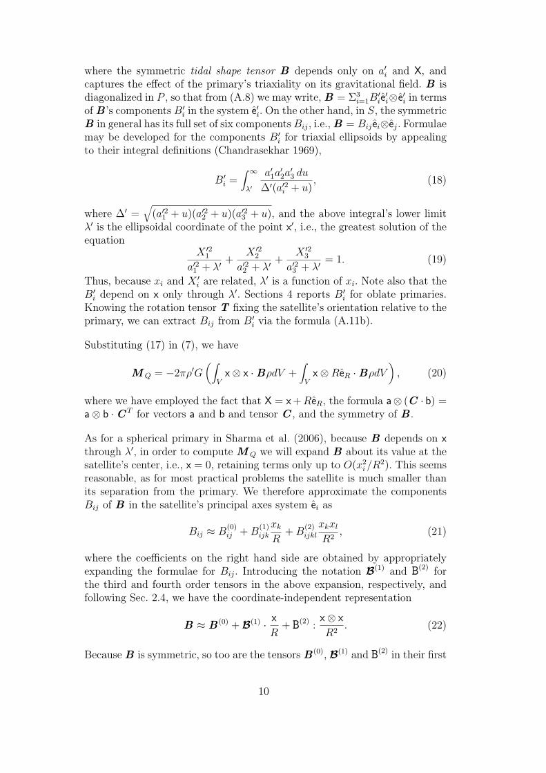
where the symmetric tidal shape tensor B depends only on a′i and X, andcaptures the effect of the primary’s triaxiality on its gravitational field. B isdiagonalized in P , so that from (A.8) we may write, B = Σ3

i=1B′ie′i⊗e′i in terms

of B ’s components B′i in the system e′i. On the other hand, in S, the symmetricB in general has its full set of six componentsBij, i.e., B = Bij ei⊗ej. Formulaemay be developed for the components B′i for triaxial ellipsoids by appealingto their integral definitions (Chandrasekhar 1969),

B′i =∫ ∞λ′

a′1a′2a′3 du

∆′(a′2i + u), (18)

where ∆′ =√

(a′21 + u)(a′22 + u)(a′23 + u), and the above integral’s lower limitλ′ is the ellipsoidal coordinate of the point x′, i.e., the greatest solution of theequation

X ′21a′21 + λ′

+X ′22

a′22 + λ′+

X ′23a′23 + λ′

= 1. (19)

Thus, because xi and X ′i are related, λ′ is a function of xi. Note also that theB′i depend on x only through λ′. Sections 4 reports B′i for oblate primaries.Knowing the rotation tensor T fixing the satellite’s orientation relative to theprimary, we can extract Bij from B′i via the formula (A.11b).

Substituting (17) in (7), we have

M Q = −2πρ′G(∫

Vx⊗ x ·BρdV +

∫V

x⊗ReR ·BρdV), (20)

where we have employed the fact that X = x +ReR, the formula a⊗ (C · b) =a⊗ b ·C T for vectors a and b and tensor C , and the symmetry of B .

As for a spherical primary in Sharma et al. (2006), because B depends on xthrough λ′, in order to compute M Q we will expand B about its value at thesatellite’s center, i.e., x = 0, retaining terms only up to O(x2

i /R2). This seems

reasonable, as for most practical problems the satellite is much smaller thanits separation from the primary. We therefore approximate the componentsBij of B in the satellite’s principal axes system ei as

Bij ≈ B(0)ij +B

(1)ijk

xkR

+B(2)ijkl

xkxlR2

, (21)

where the coefficients on the right hand side are obtained by appropriatelyexpanding the formulae for Bij. Introducing the notation B(1) and B(2) forthe third and fourth order tensors in the above expansion, respectively, andfollowing Sec. 2.4, we have the coordinate-independent representation

B ≈ B (0) + B(1) · x

R+ B(2) :

x⊗ x

R2. (22)

Because B is symmetric, so too are the tensors B (0), B(1) and B(2) in their first

10

two arguments, i.e., B(0)ij = B

(0)ji , B

(1)ijk = B

(1)jik and B

(2)ijkl = B

(2)jikl. Employing the

above expansion in (20) we find that

M Q = −2πρ′G[∫V

x⊗ x ·B (0)ρdV +∫V

x⊗ReR ·(B(1) · x

R

)ρdV

],

where we have appealed to the definition of the satellite’s center of mass, andsymmetry arguments to set the integrals with an odd number of x’s to zero.Note that B(2) does not play a role in the above equation. Following standardtensor manipulation introduced in Appendix A, we simplify the above equationto recover the basis-independent formula

M Q = −2πρ′GI ·[B (0) +

(eR ·B(1)

)T ]. (23)

Recall that eR · B(1) is a second-order tensor. We note that while I is diago-nalized in the principal axes system of the satellite, B , and so consequently,B (0) and B(1) are diagonal when viewed in P . It is helpful to specialize theabove expression to the case of a spherical primary of radius a′. Then, B (0)

and B(1) are

B (0) =2

3

a′3

R31 and B(1) = −2

a′3

R31 ⊗ eR, (24)

and we obtain for a′1 = a′2 = a′3 = a′,

M sphericalQ = −G4πa′3

3R3ρ′I · [1 − 3eR ⊗ eR] .

as obtained earlier by Sharma et al. (2006).

In order to employ the formula (23) profitably, we must develop expressionsfor B (0) and B(1). To this end we first calculate the B′i by integrating (18).From these, B ’s components in S, the Bij, are obtained by appealing to therotation tensor that relates the satellite’s and primary’s coordinate systemsS and P , respectively. The Bij are then expanded about the satellite’s centerx = 0 to yield the tensors B (0) and B(1). This process will become clear in Sec.4 when we investigate a particular satellite-primary configuration.

2.4 Orbital motion

The satellite’s orbital motion is governed by the primary’s gravitational attrac-tion. The total external gravitational force acting on the satellite is obtainedby integrating (17),

F =∫V

dF

dmdm =

∫V

bQρdV = −2πρ′G∫VB · XρdV.

11

Setting X = ReR + x, expanding B according to (22), substituting into theabove and integrating as in the previous section, we arrive at

F = −2πρ′G[mB (0) ·ReR +

1

RB(1) : I +

1

R

(B(2) : I

)· eR

],

with m being the satellite’s mass. As it follows its circular orbit around themassive primary, the satellite’s centripetal acceleration must be sustained byeR · F, so that we obtain the orbital angular velocity as

ω2 = 2πρ′GeR ·[B (0) · eR +

1

mR2

(B(1) + eR · B(2)

): I], (25)

where we have employed the symmetry of B(2) in its first two indices to simplifythe above expression. In the above, we have again neglected the satellite’s effecton the primary, taking the latter to be essentially fixed. In future applicationsto binary systems, where the components are often of comparable masses,it will be necessary to include also the primary’s motion. We note that, thistime, the tensors B (0), B(1) and B(2) are required. For a tidally-locked satellite,the orbital angular velocity equals its rotation rate, so that once ω is knownfrom the above, the spin tensor W associated with the rotation rate may beconstructed.

In the above formula, the first term is what would result if we assumed that allthe satellite’s mass were located at its center. The next two terms bring in theeffect of the satellite’s distributed mass on its orbital motion. Typically, thisis a weak perturbation, as evinced by the presence of R2 in the denominator,and we comment on its magnitude in the next subsection.

2.5 Non-dimensionalization

Collecting together (10), (12) and (23) we arrive at

σ =1

V

[−2πρGA · I − 2πρ′G

(B (0) + eR ·B(1)

)· I −W 2 · I

],

which provides the average stress in a tidally-locked triaxial satellite locatedon a circular orbit by eR with respect to a triaxial primary. The first termon the right is the average stress due to the satellite’s internal gravity, thesecond is the average tidal stress introduced by the primary, while the lastis the average “centrifugal” stress. We non-dimensionalize the above equationby rescaling time by 1/

√2πρG, and the stress by (3/20π)(2πρGm)(4π/3V )1/3,

where ρ, V and m are the satellite’s density, volume and mass, respectively.

12

We obtain

σ = −(αβ)−2/3

[W 2 + A +

1

η

(B (0) + eR ·B(1)

)]·Q , (26)

where α and β are the satellite’s axes ratios, η = ρ/ρ′ is the ratio of the satel-lite’s to the primary’s density, W and σ now represent the non-dimensionalspin and average stress tensors, respectively, and Q is a non-dimensional ten-sor derived from the inertia tensor. In S, Q takes the form

[Q ] =

1 0 0

0 α2 0

0 0 β2

, (27)

where, recall from Appendix A that square brackets denote evaluation of atensor in a coordinate system, in this case the satellite’s.

Similarly, we non-dimensionalize (25) to obtain

ω2 =1

ηeR ·

B (0) · eR +1

5q′2

(κα′β′

ηαβ

)2/3 (B(1) + eR · B(2)

): Q

, (28)

where now ω is the scaled orbital angular velocity that equals a tidally-lockedsatellite’s spin, κ = m/m′ is the ratio of the satellite’s to the primary’s mass,and q′ = R/a′1 is the scaled orbital radius. In the present application we haveassumed that the primary is much more massive than the satellite, i.e., κ� 1,and consequently we drop the corrective second-order terms, to obtain

ω2 ≈ 1

ηeR ·B (0) · eR. (29)

Note that the scaled orbit size q′ may yet be an O(1) quantity. We empha-size that the above formula, through B (0), retains the effect of the primary’sellipsoidal nature on the satellite’s orbital motion; dropping the second-orderterms in (28) is equivalent to neglecting the effect of the secondary’s dis-tributed mass.

Finally, we again make contact to the case of a spherical primary by settinga′1 = a′2 = a′3 = a′. Using (24) in the above equation to find

ω2 ≈ 1

ηeR ·

2

3

a′3

R31 · eR =

2

3

ρ′

ρ

a′3

R3,

the expected (approximate) formula for the non-dimensional orbital angularvelocity of a satellite on a circular orbit about a massive spherical primary.

13

2.6 Coordinate system

In a tidally-locked configuration, we orient the satellite’s longest principal axise1 to point away from the primary (see, e.g., Fig. 3). The principal axis e3 istaken to be normal to the orbital plane. This fixes the satellite’s principal axessystem S. We will evaluate both (26) and (29) in S. The form of the tensorQ in S is given above in (27). The gravitational shape tensor A is diagonalin S, i.e.,

[A] =

A1 0 0

0 A2 0

0 0 A3

, (30)

where, depending on the satellite’s shape, A1, A2 and A3 are given by either of(13), (14), or (15), along with (16). The non-dimensional spin tensor becomes

[W ] =

0 −W3 0

W3 0 0

0 0 0

, (31)

where, because the satellite is tidally locked,

W 23 = ω2 ≈ 1

ηeR ·B (0) · eR (32)

after substituting for ω from (29). We have neglected any “roll” about theaxis that points towards the primary. Note that W3 depends on the primary’sorientation with respect to the satellite and simplified expressions for it will beobtained separately for the two cases considered later. The tidal shape tensorB ’s matrix and so also those of B (0), B(1) and B(2), similarly depend on theorientation of the primary’s principal axes system P , and will be derived forthe example configuration in Sec. 4. Finally, the stress tensor’s components inS will be taken to be σij.

The exact volume-averaged stresses in a tidally-locked, triaxial-ellipsoidal satel-lite as it moves in a circular orbit about a triaxial ellipsoidal primary are givenby (26). However, these stresses cannot take arbitrary values for rubble pilesthat yield under high-enough shear stresses. The next section introduces ayield criterion for such granular aggregates that will help put bounds on thepossible shape and density that a rubble-pile satellite at a distance q′ from aprimary may achieve before it disrupts.

14

3 Rheology

Cohesionless rubble piles/granular aggregates (think of a gravel pile) are pri-marily characterized by their inability to withstand tensile stress and alsotheir non-zero, but finite, resistance to shear stresses. This ability to supportshear stresses is traced to both the usual interfacial friction due to particleinteraction, as well as a geometric friction due to interlocking of finite-sizedconstituents. Because of its frictional roots, the shear resistance of rubblepiles depends on internal pressure. It is further noticed that granular mate-rials when compressively loaded, suffer minimal deformation until a criticalload is reached, beyond which they deform rapidly. Keeping these features inmind, it is quite common to model granular aggregates, in the first instance,as rigid perfectly-plastic materials with an appropriate pressure-dependentyield criterion; see, e.g., Schaeffer (1987). Because here we are concerned withonly equilibrium shapes, and not dynamical behavior post-yield, we will onlyintroduce yield criteria relevant for a granular aggregate and not model theaggregate’s behavior after it yields. More complete discussions of modelinggranular materials as rigid perfectly-plastic materials, addressing also theirpost-yield flow, are provided in Sharma (2004) and Sharma et al. (2008).

Pressure-dependent yield criteria appropriate for granular materials are pro-vided by both the Mohr-Coulomb and the Drucker-Prager failure laws (Chenand Han 1988). The Mohr-Coulomb yield criterion is stated in terms of theextreme principal stresses

σmax − kMCσmin ≤ 0, (33)

where kMC is related to the internal friction angle φF by

kMC =1 + sinφF1− sinφF

. (34)

Here, we prefer to employ the Drucker-Prager yield criterion as its smoothnessfacilitates numerical calculations, though a brief comparison with the resultsof a Mohr-Coulomb material is provided in Sec. 6.2. To formulate the Drucker-Prager failure rule we define the pressure p

p = −1

3tr σ, (35)

where ‘tr’ denotes the trace of the tensor, and the deviatoric stress s

s = σ + p1. (36)

The Drucker-Prager yield condition can then be written as

|s|2 ≤ k2p2, (37)

15

where |s| indicates the magnitude of the deviatoric stress as given by

|s|2 = sijsij,

applying the summation convention, and

k =2√

6 sinφF3− sinφF

, (38)

defined so that the Drucker-Prager yield surface is the outer envelope of theMohr-Coulomb yield surface corresponding to the same friction angle φF . Asthe friction angle lies between 0o and 90o, 0 > k >

√6. Finally, in terms of

the three principal stresses σi, the definition above for |s| may be put into theilluminating form

|s|2 =1

3

[(σ2 − σ3)

2 + (σ3 − σ1)2 + (σ1 − σ2)

2]

=2

3

(τ 21 + τ 2

2 + τ 23

), (39)

where τi = (σj − σk)/2, (i 6= j 6= k) are the principal shear stresses at apoint. Thus, |s| may be thought of as a measure of the “total” local shearstress. Thus, the Drucker-Prager yield criterion (37), along with (38), puts alimit on the allowable local shear stresses in terms of the local pressure andthe internal friction angle. This interpretation will be found useful when weexplore the yielding modes of tidally-locked satellites later.

4 Example: Satellites of oblate primaries

We now commence to explore the equilibrium landscape of rubble-pile satel-lites. So far we have at most assumed that the tidally-locked satellite followsa circular path around an ellipsoidal primary. For clarity, we will now restrictourselves to the geometry shown in Fig. 3, viz., an oblate primary with thetriaxial-ellipsoidal satellite’s orbit lying in the primary’s equatorial plane. Re-call that for a tidally-locked configuration to be stable, the satellite’s long-axisa1 must point towards the primary. This configuration is of immediate impor-tance for planetary satellites.

The average value of the stresses evaluated in S within a tidally-locked el-lipsoidal satellite on a circular orbit is obtained from (26) along with (27),(30), (15) (or (13), or (14)), (31) and (32). In addition, we require expressionsfor the tensors B (0) and B(1) in the satellite’s principal coordinate system.These two tensors are obtained according to the prescription outlined in thelast paragraph of Sec. 2.3, and will be apparent in the following section. Notethat because we have used the approximate expression (32) for W3 rather than

(28), we will not require B(2). The stresses finally obtained, along with the yield

16

e1’ e

1

e2’

e3’

e2

e3

RP

S

Primary

SatelliteOrbital plane eR

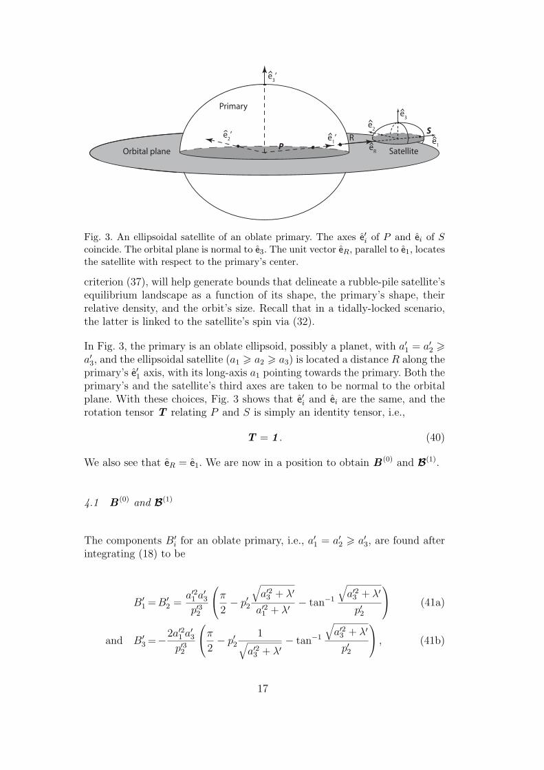
Fig. 3. An ellipsoidal satellite of an oblate primary. The axes e′i of P and ei of Scoincide. The orbital plane is normal to e3. The unit vector eR, parallel to e1, locatesthe satellite with respect to the primary’s center.

criterion (37), will help generate bounds that delineate a rubble-pile satellite’sequilibrium landscape as a function of its shape, the primary’s shape, theirrelative density, and the orbit’s size. Recall that in a tidally-locked scenario,the latter is linked to the satellite’s spin via (32).

In Fig. 3, the primary is an oblate ellipsoid, possibly a planet, with a′1 = a′2 >a′3, and the ellipsoidal satellite (a1 > a2 > a3) is located a distance R along theprimary’s e′1 axis, with its long-axis a1 pointing towards the primary. Both theprimary’s and the satellite’s third axes are taken to be normal to the orbitalplane. With these choices, Fig. 3 shows that e′i and ei are the same, and therotation tensor T relating P and S is simply an identity tensor, i.e.,

T = 1 . (40)

We also see that eR = e1. We are now in a position to obtain B (0) and B(1).

4.1 B (0) and B(1)

The components B′i for an oblate primary, i.e., a′1 = a′2 > a′3, are found afterintegrating (18) to be

B′1 =B′2 =a′21 a

′3

p′32

π2− p′2

√a′23 + λ′

a′21 + λ′− tan−1

√a′23 + λ′

p′2

(41a)

and B′3 =−2a′21 a′3

p′32

π2− p′2

1√a′23 + λ′

− tan−1

√a′23 + λ′

p′2

, (41b)

17

where p′2 =√a′21 − a′23 , and the ellipsoidal coordinate λ′ is given by (19). Note

that upon dividing by a′31 we can express (41) in terms of the scaled orbitalradius q (= R/a′1) and the primary’s axes ratio β′ (= a′3/a

′1). Employing (40)

with the tensor coordinate transformation formulae (A.11b), we obtain

Bij = B′iδij (no sum), (42)

i.e., because P and S are identical, so too are B ’s components in them.

We next solve (19) approximately to find λ′ at a point X = x +Re1 within thesatellite. To this end we note from Fig. 3 (or, equivalently (40) and (A.11a))that xi = x′i. To order x2

i /R2, we obtain

λ′ = λ′(x) ≈ λ′0 +R2

{2x1

R+

1

R2

(x2

1 + x22 +

R2

R2 − p′22x2

3

)}, (43)

whereλ′0 = R2 − a′21 (44)

is the value of λ′ at the satellite’s center, i.e., at x = 0. We substitute theabove approximation into the formulae for Bij obtained from (42) and (41),and expand up to O(x2

i /R2) to find an expression similar to (21). This yields

the components of the tensors B (0), B(1) and B(2) in S, the satellite’s coordinatesystem. In particular, B (0) is diagonal with B

(0)ii = B′i|λ′=λ′

0, so that (41) yields

B(0)11 = B

(0)22 =

β′

(1− β′2)3/2

π2−q′o

√(1− β′2)q′2

− tan−1 q′o√1− β′2

(45a)

≈ 2

3

β′

q′3+

1

5

β′(1− β′2)q′5

+3

28

β′(1− β′2)2

q′7...

and B(0)33 = − 2β′

(1− β′2)3/2

(π

2−√

1− β′2q′o

− tan−1 q′o√1− β′2

), (45b)

≈ 2

3

β′

q′3+

3

5

β′(1− β′2)q′5

+15

28

β′(1− β′2)2

q′7...

where we have chosen to express quantities in terms of the primary’s axes ratioβ′, the satellite’s scaled orbital radius q′, and q′2o = q′2 + β′2− 1. Similarly, theonly non-zero components of B(1) are

B(1)111 = B

(1)221 = − 2β′

q′2q′o≈ −2

β′

q′3− β′(1− β′2)

q′5− 3

4

β′(1− β′)2

q′7+ ... (46a)

and B(1)331 = −2β′

q′3o≈ −2

β′

q′3− 3

β′(1− β′2)q′5

− 15

4

β′(1− β′)2

q′7+ ... . (46b)

In the above, we have provided expansions in orders of 1/q′ to illustrate thatthe oblateness β′ enters linearly at the first order. For β′ ≈ 1 and/or large

18

enough q′’s, as is the case with most known planetary satellite systems, re-taining only the first terms is found sufficient (see Sec. 5). This simplification

prompts the introduction of an equivalent distance q′ = q′ (η/β′)1/3 that, inthe leading-order approximation, absorbs the effect of the density ratio η andthe primary’s axes ratio β′. However, in Sec. 4.3, we will investigate the equi-librium landscape while employing the exact expressions for B

(0)ij and B

(1)ijk

provided above. In this case, q′ does not capture the effects of η and β′ intheir entirety, but because it does do so to first order, we will express resultsin terms of q′ rather than q′.

4.2 The spin W3

With eR = e1, from (32), we obtain

W 23 =

1

ηB

(0)11 , (47)

with B(0)11 , given by (45a), capturing the effect of the primary’s asphericity.

4.3 Equilibrium landscape

We proceed to explore the equilibrium of an oblate primary’s rubble-pile satel-lite, as shown in Fig. 3. To this end, we utilize (26) to express the averagestresses within the satellite in its principal axes system ei. We find

σ1 = −{−W 2

3 + A1 +1

η

(B

(0)11 +B

(1)111

)}(αβ)−2/3,

σ2 = −α2

(−W 2

3 + A2 +1

ηB

(0)11

)(αβ)−2/3

and σ3 = −β2

(A3 +

1

ηB

(0)33

)(αβ)−2/3,

where η = ρ/ρ′ is the density ratio, α and β the satellite’s axes ratios, and theexpressions for Ai are given by appropriate formulae in Sec. 2.2, while thoseof B

(0)ij and B

(1)ijk by (45) and (46), respectively. The primary’s oblateness β′

and the size of the satellite’s orbit q′ (or, equivalently, q′) affect the stresses

through the terms B(0)11 , B

(0)33 and B

(1)111. On substituting for W3 from (47), the

19

above expressions simplify further to become

σ1 = −(A1 +

1

ηB

(1)111

)(αβ)−2/3, (49a)

σ2 = −α2A2(αβ)−2/3 (49b)

and σ3 = −β2

(A3 +

1

ηB

(0)33

)(αβ)−2/3. (49c)

The stresses above must satisfy the Drucker-Prager yield criterion (37) in orderfor the satellite to exist in equilibrium. At equilibrium, equality holds in (37),thereby providing a relationship between the satellite’s axes ratios α and β, itsinternal friction angle φF , the equivalent orbit size q′, the primary’s oblatenessβ′, and the density ratio η. The satellite’s equilibrium is thus governed byseveral variables. The aim is to identify the limits placed on the satellite’sorbital radius q′ by the remaining five parameters φF , α, β, β

′ and η. Thisis a high-dimensional and complicated relationship, and we will explore itgraphically by taking appropriate two-dimensional sections.

We first fix the primary’s oblateness β′ at 0.8 and the density ratio η to 0.5. Thesatellite is thus half as dense as the primary. With these choices, q′ ≈ 1.17 q′.The critical equivalent orbital radius q′ is now regulated only by the satellite’sshape in terms of its axes ratios α and β, and the internal friction angle φF .At any given φF , the set of q′, α and β that ensure the satellite’s equilibrium,i.e., produce (average) stresses that do not violate the yield criterion, definea three-dimensional region in α − β − q′ space. Different φF yield differentregions. For each friction angle, the critical surfaces delineating the associatedregion, provide us with limits on q′ given the satellites α and β. Conversely,knowing the orbit’s size q′ constrains the satellite’s α and β. The critical sur-faces themselves are obtained by assuming equality in the yield criterion (37).We probe this three-dimensional region via planes obtained by either fixing α,or relating α to β. Thus, each such two-dimensional section, henceforth calledan α-section, corresponds to a class of self-similar ellipsoidal satellites. Fivesuch planar sections corresponding to α = 0.5 and 0.75, and to oblate (α = 1),prolate (α = β) and average-triaxial (α = (1 + β)/2) ellipsoids are shown inFigs. 4 and 5. We discuss them next. We reiterate that while exploring theα− β − q′ space, β′ = 0.8 and η = 0.5.

In the α-sections of Figs. 4 and 5, the critical surfaces corresponding to afriction angle φF now appear as curves. On these curves, q′ is related onlyto β, and this relationship may be obtained from the yield criterion (37)at equality. These curves help define regions in β − q′ space within which asatellite can survive as a rubble pile, provided its internal friction is at leastas great as that due to the defining curve’s associated φF . Thus, for example,a satellite with α = 0.5 and a friction value of φF = 20o may only existin equilibrium within the shaded region of Fig. 4(a). We also see that the

20

1

2

3

4

5

0.1 0.2 0.3 0.4 0.5Axes ratio, β = a3 /a1

Equ

ival

en

t d

ista

nce

, q

’ = q

‘(η/β

’)1/3

40o 10o

20o30o

90o

1o5o3o

Darwin ellipsoid

(a) α = 0.5

1

2

3

4

5

0.1 0.2 0.3 0.4 0.5 0.6 0.7

Axes ratio, β = a3 /a1

Darwin ellipsoid

1o

40o

3o5o10o

20o

30o

90o

2.57

Equ

ival

ent

dis

tan

ce,

q’ =

q‘(η

/β’)1/

3

0.75

(b) α = 0.75

Fig. 4. The equilibrium landscape in β − q′ space as viewed on the sections α = 0.5and 0.75. The number next to a critical curve is the associated friction angle φF .The primary’s oblateness β′ = 0.8 and the density ratio η = 2. The axis ratio β’supper limit is set by the inequality β 6 α. The Darwin ellipsoid at φF = 0o isindicated by a ‘+’ symbol.

equilibrium region for any φF encloses those of all smaller friction angles. Thissimply reflects that increasing internal friction allows the body to withstandgreater shear stresses. An important consequence of this is that constraintsreflected by equilibrium landscapes such as Figs. 4 and 5 impose necessary,but not sufficient, requirements on the satellite to persist in equilibrium. This,for example, means that any satellite with given physical and orbital data willrequire an internal friction at least as great as the φF corresponding to thecritical curve that passes through its location in β − q′ space.

In both the α-sections shown in Fig. 4, we see that the allowed regions becomeincreasingly smaller as the friction angle decreases, reducing ultimately toa point when φF becomes zero. This is indicated by a ‘+’ symbol. Recallthat φF = 0o corresponds to inviscid fluids, so that this point is, in fact, the

21

1

2

3

4

5

0.1 0.2 0.3 0.4 0.5 0.6 0.7 0.8 0.9 1Axes ratio, β = a3 /a1

1o

40o

3o

5o

10o20o30o

90o

Equ

ival

en

t d

ista

nce

, q

’ = q

‘(η/β

’)1/3

(a) Oblate satellite with α = 1

1

2

3

4

5

0.1 0.2 0.3 0.4 0.5 0.6 0.7 0.8 0.9 1Axes ratio, β = a3 /a1

1o

40o

3o5o

10o

20o

90o

1o

3o

5o

10o

20o

30o

Equ

ival

en

t d

ista

nce

, q

’ = q

‘(η/β

’)1/3

1.71

(b) Prolate satellite with α = β

1

2

3

4

5

0.1 0.2 0.3 0.4 0.5 0.6 0.7 0.8 0.9 1Axes ratio, β = a3 /a1

1o

40o

3o

5o10o

20o30o

90o

Equ

ival

en

t d

ista

nce

, q

’ = q

‘(η/β

’)1/3

(c) Triaxial satellites with α = (1 + β)/2

Fig. 5. Continued from Fig. 4. The equilibrium landscape in β−q′ space as viewed onsections corresponding to oblate, prolate and average-triaxial-ellipsoidal satellites.For these shapes, there is no solution at φF = 0o. See also Fig. 4’s caption.

22

intersection of the first Darwin sequence of ellipsoids (Chandraskhar 1969)with the planes α = 0.5 or α = 0.75. In contrast, note from Fig. 5 thatoblate, prolate, or average-triaxial (α = (1+β)/2), inviscid tidally-locked, fluidellipsoids do not exist. To be completely precise, the Darwin sequence obtainedhere is for a primary whose oblateness β′ is taken fixed and not necessarilyrelated to any spin that the primary may itself have. In the Darwin problem,as considered by Chandrasekhar (1969), the primary was a fluid Maclaurinspheroid. But, because the focus here is on the satellite’s equilibrium, wewill not belabor this distinction, and instead label the solution obtained forφF = 0o, when it exists, as a Darwin ellipsoid.

For the α-sections displayed in Fig. 4, the equilibrium regions are closed atlow friction angles. This is not the case at higher φF ’s, or for any friction valuefor the oblate/prolate/average-triaxial shapes considered in Fig. 5. Typically,for any φF , at a fixed axes ratio β, there is both a lower and an upper limit tothe size of a rubble-pile satellite’s orbit. Comparing Figs. 4(a) - 5(c), we alsosee that for any φF , the β-range over which the upper limit exists, reduceswith increasing α; the equilibrium regions for the oblate case in Fig. 5(a) havealmost no upper bounds. Physically, the lower bound corresponds to failuredriven by increased tidal and centrifugal stresses. Closer to the primary, boththese forces increase due to stronger tidal interaction with the primary and ahigher rotation rate. Thus, we identify this failure mode as tidal disruption.This mode has close analogy with the upper rotational disruption curve thatoccurs in the equilibrium landscape of rubble piles in pure spin (Sharma etal. 2008). The upper bound, on the other hand, is associated with the body’sinability to withstand its own gravity. We term this as gravitational collapse.At distances far away from the primary, tidal and centrifugal forces reduce.The latter, because the satellite is assumed to be spin-locked. In such condi-tions, internal gravity comes to dominate, and may cause yielding. This upperbound should be compared with the lower critical curve for spinning rubblepiles (Sharma et al. 2008).

Equilibrium regions such as shown in Figs. 4 and 5 are useful to put boundson the satellite’s physical parameters such as shape or internal structure. As afirst illustration, consider a satellite with α = 0.75 and β = 0.4 moving on anorbit with q′ = 2.57 about an oblate primary with β′ = 0.8 and η = 0.5. Suchan object may be located on the section of Fig. 4(b), as shown by the filledcircle. We see that this body lies outside the φF = 10o curve but within theregion where rubble piles with an internal friction of φF = 20o may survive.This allows us to conclude that the satellite in question must be composedof a material with a friction angle greater than 10o. This could be a rubblepile, as such aggregates typically have φF ≈ 30o (Nedderman 1992, p. 25,Table 3.1). Conversely, if a body’s orbit were known, and we were confidentabout the object being a rubble pile, we could employ sections such as thosein Figs. 4 and 5 to constrain its shape. For example, assuming that φF = 30o

23

is appropriate for granular aggregates, we may conclude from Fig. 5(b) thata tidally-locked rubble pile at a distance q′ = 1.71 from an oblate primarywith β′ = 0.8 and η = 0.5, can be a prolate ellipsoid with α = β > 0.69.This is indicated by an open circle in Fig. 5(b). Any smaller β would placethe satellite outside the φF = 30o curve, contradicting our assumption aboutthe maximum shear strength of granular aggregates. Finally, if one of the axesratios were known, a similar analysis may be carried out to constrain the otherratio.

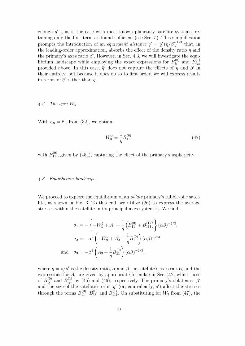
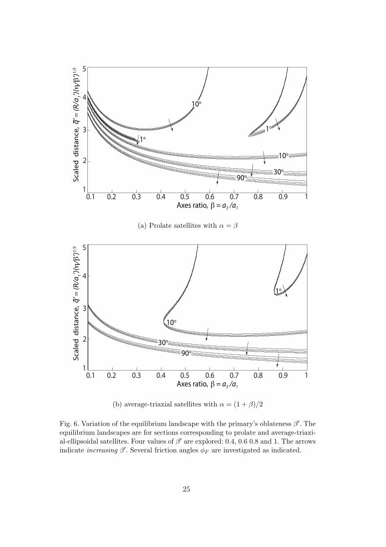
Next, we explore how the satellite’s equilibrium landscape is affected by theprimary’s oblateness β′. To this end, we restrict the satellite to be either aprolate (α = β) or an average-triaxial (α = (1+β)/2) ellipsoid, and also fix thedensity ratio η at 0.5. Figure 6 plots the critical curves corresponding to severalfriction angles for β′ equalling 1, 0.8, 0.6 and 0.4. The value β′ = 1 correspondsto a spherical primary, in which case the first Darwin problem reduces tothe Roche problem (see Sec. 5). The arrows in Fig. 6 indicate directions ofincreasing β′. It is seen that the equilibrium region in β − q′ space remainsessentially unchanged, especially at low friction angles. This is due to ouremploying the equivalent distance q′ = q′ (η/β′)1/3, which to first order absorbsthe effects of both density ratio η and the primary’s oblateness β′. That thecritical curves do not coincide, but in fact move downwards as the primarybecomes “flatter”, i.e., β′ lessens, is due to our employing exact formulae forB

(0)ij and B

(1)ijk; see (45) and (46). Because q′ ∝ R/a′1β

′1/3 ∝ R (ρ′/m′)1/3, weconclude that, in physical space, the critical distance beyond which a satellitewith fixed axes ratio β may exist increases as the primary flattens, as long asm′ and ρ′ remain fixed. This may be traced directly to the fact that, for thesame mass and density, a flatter primary’s in-plane tidal influence persists forgreater distances.

The effect of β′ will have important consequences for satellite systems withsignificant ring mass, or satellites of flattened asteroids/planets. Typically,though, asteroids tend to be prolate or triaxial rather than oblate, in whichcase the calculations above need to reworked for prolate/triaxial primaries, ina manner similar to that of an oblate central body.

Finally, we investigate the impact of changing the density ratio η = ρ/ρ′. Thistime, we consider only a prolate satellite. The results are shown in Fig. 7(a).The density ratio varies as 0.5, 1, 1.5 and 2, i.e., from a situation where thesatellite is half as dense as the primary, to one where it is twice as dense.Both ends of this spectrum are of physical interest. The primary’s oblatenessβ′ was fixed at 0.8, and four friction angles for each η were considered. Thearrows in Fig. 7(a) indicate directions of increasing η. We have truncated crit-ical curves that fell below q′ = 1.1. We again observe that in β − q′ space,the allowed equilibrium region remains almost unaltered. This, as mentionedearlier, is a reflection of the fact that q′ absorbs the leading order effect of η

24

1o

10o

30o

90o

10o

1o

1

2

3

4

5

0.1 0.2 0.3 0.4 0.5 0.6 0.7 0.8 0.9 1

Axes ratio, β = a3 /a1

Sc

ale

d

dis

tan

ce

, q

’ = (

R/a

1’)

(η/β

’)1

/3

(a) Prolate satellites with α = β

1o

30o

90o

10o

1

2

3

4

5

0.1 0.2 0.3 0.4 0.5 0.6 0.7 0.8 0.9 1

Axes ratio, β = a3 /a1

Sc

ale

d

dis

tan

ce

, q

’ = (

R/a

1’)

(η/β

’)1

/3

(b) average-triaxial satellites with α = (1 + β)/2

Fig. 6. Variation of the equilibrium landscape with the primary’s oblateness β′. Theequilibrium landscapes are for sections corresponding to prolate and average-triaxi-al-ellipsoidal satellites. Four values of β′ are explored: 0.4, 0.6 0.8 and 1. The arrowsindicate increasing β′. Several friction angles φF are investigated as indicated.

25

1o

10o

30o

90o

10o

1o

1

2

3

4

5

0.1 0.2 0.3 0.4 0.5 0.6 0.7 0.8 0.9 1Axes ratio, β = a3 /a1

Sc

ale

d

dis

tan

ce

, q

’ = (

R/a

1’)

(η/β

’)1

/3

q’ = 1.1

(a) Prolate satellites with α = β

1

2

3

4

5

0.1 0.2 0.3 0.4 0.5 0.6 0.7 0.8 0.9 1

Axes ratio, β = a3 /a1

1o

10o

30o

90o

1.1

Sc

ale

d d

ista

nc

e,

q’ =

R/a

1’

(b) Prolate satellites with α = β

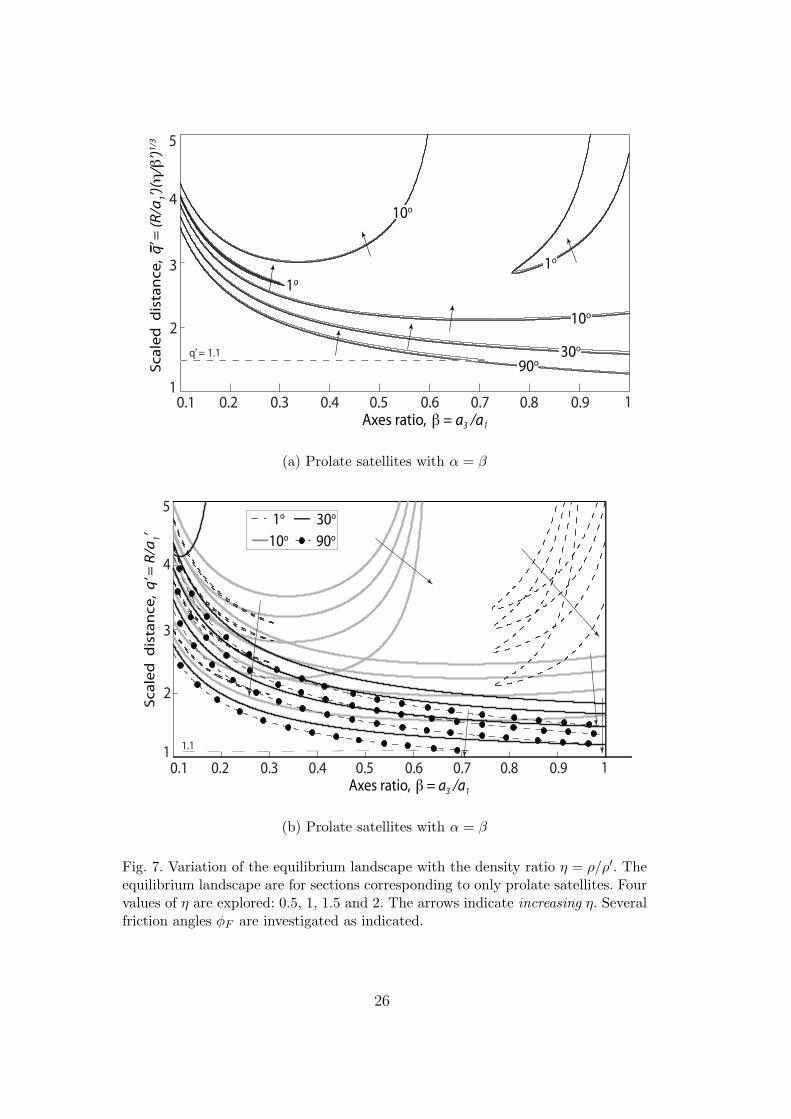
Fig. 7. Variation of the equilibrium landscape with the density ratio η = ρ/ρ′. Theequilibrium landscape are for sections corresponding to only prolate satellites. Fourvalues of η are explored: 0.5, 1, 1.5 and 2. The arrows indicate increasing η. Severalfriction angles φF are investigated as indicated.

26

variations. In physical space, because q′ ∝ q′/η1/3, the equilibrium region forany φF moves further away from the primary as η decreases, as is borne outby Fig. 7(b) where we plot the critical curves in β− q′ space. This behavior isunderstood easily by recognizing that lower η corresponds to greater primarymass, or, correspondingly lower satellite density. While the former circum-stance increases the disruptive tidal effect of the primary, the latter reducesthe self-gravitational forces that hold the rubble-pile satellite together. Thus,to persist in equilibrium, a granular aggregate has to move further away froma denser primary. Conversely, a denser satellite, with greater self-gravity, cancome closer to its primary.

4.4 Discussion

Above, we obtained critical bounds on the equivalent orbital radius q′ of atidally-locked rubble-pile ellipsoidal satellite as it moves on a circular pathabout an oblate primary. Equivalently, the satellite’s orbit and internal strengthconstrained its shape. Employing stresses from (49) in conjunction with theDrucker-Prager yield criterion (37), we generated limits for q′ as a functionof the satellite’s internal friction φF , its shape α and β, the primary’s oblate-ness β′, and the density ratio η of the primary to the satellite. We exploredthis high-dimensional dependency via appropriate two-dimensional planes (α-sections) that correspond to self-similar ellipsoidal shapes of the satellite. Afterfixing β′ and η, on any α-section, the friction angle φF identifies a region inβ − q′ space within which a rubble-pile with at least that much φF may existin equilibrium. This region, except for φF = 90o, had both lower and upperlimits. At φF = 90o, the upper limit moved to infinity. Both these boundswere understood in terms of the interplay between the debilitating tidal andcentrifugal stresses and the fortifying self-gravity, and tracing the source ofhigh shear stresses at failure. Analogies were drawn with previous equilibriumanalysis for a rubble pile in pure spin (Sharma et al. 2008). We also saw howthese equilibrium landscapes help constrain an object’s physical and orbitalparameters. Finally, the effect of varying the primary’s oblateness and chang-ing the density ratio was also noted. Typically, with decreasing β′ and/or η,the allowed equilibrium region moves away from the primary. For the samemass, a more flattened planet, i.e., with lower β′, has greater disruptive tidalinfluence. Similarly, low-density objects tend to disrupt more easily, as tidaleffects then dominate the self-gravity holding the satellite together.

As mentioned in the Introduction, volume-averaging, in the case of cohesion-less rubble piles in pure spin (Sharma et al. 2008), precisely matched theexact results of Holsapple (2001) that were in turn based on the method oflimit analysis (Chen and Han 1988). Here too, we predict that the constraintson q′ obtained above by volume-averaging will be the same as those from limit

27

analysis. Indeed, this is the case for the Roche problem discussed in Sec. 5.However, caution must be exercised, because as mentioned in Sharma et al.(2008), there is no known fundamental reason for this coincidence betweena volume-averaged approach and limit analysis. It is also unclear when andunder what conditions will the outcomes of these two methods agree. In fact,if the granular aggregate had a small amount of cohesion, the conclusions oflimit analysis and volume-averaging will differ. However, recently Holsapple(2008) has shown that yield predictions predicated on average stresses are anupper bound to the exact results of limit analysis for rigid-plastic materials,i.e., if a rigid-plastic object yields on average, it will definitely yield.

Finally, because no satellite or primary is a perfect ellipsoid, in order profitablyto utilize the constraints obtained above, it is necessary to note the effect ofsurface irregularities. Deviations in the shape of both these bodies from theirbest-fit ellipsoids will introduce perturbations in the stress field obtained byotherwise approximating these bodies as ellipsoids. If the unevenness is on ascale larger than the constitutive particle size of the granular aggregate, thenthe perturbation in the stress field will locally violate the yield criterion. Thus,for a rubble-pile satellite modeled as above to survive, it is necessary that themodel problem employing nominal 1 ellipsoids for both the satellite and theprimary satisfy the conditions for equilibrium obtained above. In other words,for a satellite to exist as a rubble pile with some internal friction angle φF ,a viable necessary condition is for its associated ellipsoidal shapes to satisfythe bounds associated with an appropriately smoothened primary and thatφF (and that ellipsoidal shape).

We now proceed to two applications of the theory developed above. We firstspecialize to the important case of a spherical primary to recover a gener-alization appropriate for granular aggregates of the classical Roche problem,and employ it to investigate the two moons of Mars. In the process, we willalso make contact with previous work in this area, and also results due to thealternate Mohr-Coulomb yield criterion. Satisfactory results in this simplercase will engender confidence in our more general development, which is thenemployed to investigate suspected rubble-pile satellites of the giant planets,explicitly accounting for the primary’s flattening.

5 Application: The Roche problem

In the special case when the primary is a sphere, we recover the classical Rocheproblem adapted to solid bodies. More precisely, we obtain limits on the orbitsthat a rubble-pile satellite of a spherical planet may occupy depending on its

1 Obtained by smoothing irregularities over several particle lengths

28

internal friction. For a spherical planet, we set β′ = 1 in (45) and (46) and

substitute for B(1)111 and B

(0)33 in (49) to obtain the average stresses as

σ1 = −(A1 −

2

q′3

)(αβ)−2/3, (50a)

σ2 = −α2A2(αβ)−2/3 (50b)

and σ3 = −β2

(A3 +

2

3q′3

)(αβ)−2/3, (50c)

where now q′ = q′η1/3 is the equivalent distance, and we recall that the ex-pressions for Ai are given in Sec. 2.2. Employing the above stresses with theDrucker-Prager yield criterion as before, we obtain regions in shape (β) –equivalent distance (q′) space wherein a tidally-locked rubble-pile satellite ofa spherical planet may exist in equilibrium.

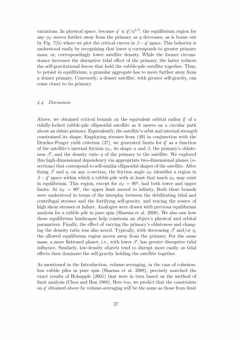
Figure 8 displays the results for an oblate satellite, wherein α = 1 andA1 = A2.We see that a fluid oblate satellite cannot exist, and this is consistent withRoche’s result (see Chandrasekhar 1969). As the friction angle increases, theregion within which a satellite with a given axes ratio β may exist as a rubblepile increases. We note that even when consisting of a material with infinitefriction, i.e., φF = 90o, an oblate satellite will fail if it gets close enough tothe planet. Note that when the friction angle is 90o, an object can only fail intension. This case will be revisited in Sec. 5.2.

At any given axes ratio β and friction angle φF , there is typically only a lowerlimit to how close the satellite may come. Exceptions occur over a small β-range at lower friction angles, e.g., for 0.58 6 β 6 0.62 at φF = 10o. Asbefore, falling below the lower value for q′ corresponds to yielding due to highshear stresses from increased tidal interaction. Crossing the upper limit, whenit exists, indicates an inability of the object to sustain its self-gravitationalstresses.

Equilibrium landscapes for other combinations of axes ratios α and β may besimilarly constructed and explored. We employ one such selection to investi-gate the moons of Mars next.

5.1 Mars

The red planet Mars is nearly spherical (β′ = 0.99) and has two satellites,Phobos and Deimos. There are suggestions, based on their physical proper-ties such as density, albedo, color and reflectivity that are similar to C-typeasteroids, that both these moons are captured asteroids. Burns (1992), how-ever, notes that the calculated histories of orbital evolution of these moons

29

0.1 0.2 0.3 0.4 0.5 0.6 0.7 0.8 0.9 1

Axes ratio, β = a3 /a1

1

2

3

4

Dis

tan

ce

in

q

’ = q

’η1

/3

5

1o

40o

3o

5o

10o20o

30o

90o

Fig. 8. The equilibrium landscape of a spherical primary’s rubble-pile oblate satel-lite. Curves correspond to various friction angles φF , as shown by adjacent numbers.

provides contradictory evidence to the effect that these moons in fact origi-nated in circum-Martian orbit. Nevertheless, for the moment, we will proceedwith the assumption that the low density and high porosity of these objectsreflects a granular interior. Table 1 lists orbital and physical parameters forthese two Martian satellites obtained from NASA’s Solar System Dynamicswebsite (http://ssd.jpl.nasa.gov) and Duxbury and Callahan (1989).

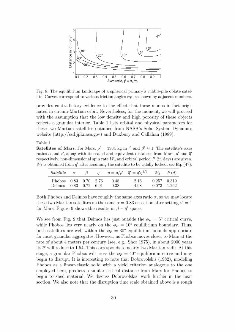
Table 1Satellites of Mars. For Mars, ρ′ = 3934 kg m−3 and β′ ≈ 1. The satellite’s axesratios α and β, along with its scaled and equivalent distances from Mars, q′ and q′

respectively, non-dimensional spin rate W3 and orbital period P (in days) are given.W3 is obtained from q′ after assuming the satellite to be tidally locked; see Eq. (47).

Satellite α β q′ η = ρ/ρ′ q′ = q′η1/3 W3 P (d)

Phobos 0.83 0.70 2.76 0.48 2.16 0.257 0.319Deimos 0.83 0.72 6.91 0.38 4.98 0.073 1.262

Both Phobos and Deimos have roughly the same axes ratio α, so we may locatethese two Martian satellites on the same α = 0.83 α-section after setting β′ = 1for Mars. Figure 9 shows the results in β − q′ space.

We see from Fig. 9 that Deimos lies just outside the φF = 5o critical curve,while Phobos lies very nearly on the φF = 10o equilibrium boundary. Thus,both satellites are well within the φF = 30o equilibrium bounds appropriatefor most granular aggregates. However, as Phobos moves closer to Mars at therate of about 4 meters per century (see, e.g., Shor 1975), in about 2000 yearsits q′ will reduce to 1.54. This corresponds to nearly two Martian radii. At thisstage, a granular Phobos will cross the φF = 40o equilibrium curve and maybegin to disrupt. It is interesting to note that Dobrovolskis (1982), modelingPhobos as a linear-elastic solid with a yield criterion analogous to the oneemployed here, predicts a similar critical distance from Mars for Phobos tobegin to shed material. We discuss Dobrovolskis’ work further in the nextsection. We also note that the disruption time scale obtained above is a rough

30

1o

40o

3o

5o10o20o30o

Phobos

Deimos

90o

0.1 0.2 0.3 0.4 0.5 0.6 0.7 0.831

2

3

4

Dis

tan

ce

in

q’=

q’η

1/3

Axes ratio, β = a3 /a1

5

Fig. 9. The two Martians shown on the planar section α = 0.83 of the three-dimen-sional α−β−q′ space. The primary’s axes ratio β′ was set to one. Curves correspondto particular choices of the friction angle φF , as indicated by the adjacent numbers.The Darwin ellipsoid associated with φF = 0o is indicated by a ‘+’ symbol. Theupper limit is set by the requirement β 6 α.

estimate; the actual time may well be shorter as Phobos accelerates as itmoves closer to Mars. Finally, compared to Phobos, Deimos is much moreconveniently placed to survive as a rubble pile.

We next compare the results for the Roche problem with answers due to adifferent choice of the yield criterion, and also make contact with previousresearch.

5.2 Alternate yield criteria and previous work

In Sec. 3 we discussed the Mohr-Coulomb failure law as an alternative to theDrucker-Prager yield criterion. Because both these yield criteria are exten-sively employed in geophysical research (Chen and Han 1988), we provide aquick comparison between their predictions. In Fig. 10 we juxtapose the equi-librium landscape for a tidally-locked prolate rubble pile in orbit about a spher-ical planet as obtained from both the Mohr-Coulomb and the Drucker-Prageryield criteria. We see that the equilibrium landscape due to the Mohr-Coulombfailure law is contained within that of the Drucker-Prager yield criterion. Thisfeature was also noted for the case of a granular aggregate in pure spin bySharma et al. (2008). A consequence is that objects that are suspected not tobe rubble piles when tested with a Mohr-Coulomb criterion, may be perfectlyacceptable when examined as Drucker-Prager materials. As mentioned earlier,Sharma et al. (2006) have noted that numerical simulations suggest that theDrucker-Prager yield criterion may be better suited for granular aggregates.Hence, we preferred the Drucker-Prager criterion in this work.

The Mohr-Coulomb yield criterion provides an important point of contactwith the earlier work of Davidsson (2001). He found the Roche limit for solid

31

1

2

3

4

5

6

0.1 0.2 0.3 0.4 0.5 0.6 0.7 0.8 0.9 1

Dis

tan

ce in

q’ =

q’η

1/3

Axes ratio, β = a3 /a1

1o

5o

10o

20o30o

Mohr-Coulomb

Drucker-Prager

5o

20o

90o

30o

10o

1o

Fig. 10. The equilibrium landscape of a prolate satellite due to applications of theMohr-Coulomb and Drucker-Prager yield criteria. Curves are drawn for variousfriction angles as shown.

axi-symmetric objects in orbit about a spherical primary by assuming firsta failure plane within the satellite. Parts of the object on either side of thisfailure plane were treated as separate entities that interact across this plane.Stresses were calculated by dividing the net interaction force by the plane’sarea. Davidsson (2001) assumed that the object failed when the stress nor-mal to the failure plane surpassed the constituent material’s tensile strength.Amongst all possible planes, the critical failure plane was that plane acrosswhich the interaction stress first became zero. This method of stress analysisis reminiscent of basic engineering mechanics, and is often useful for obtain-ing first estimates. It neglects local variations of stress, and instead workswith stress averages over larger cross-sections. In the case of prolate ellipsoids,Davidsson (2001) found the critical failure plane to be the symmetry planeperpendicular to the long axis that itself points towards the primary. Assum-ing that the satellite has no tensile strength, Davdisson’s (2001) results maybe put into the following form:

q′D =(

4π

ε

)1/3

,

32

where q′D is the closest a satellite may to a planet before failing, and

ε =4πf

(f 2 − 1)3/2ln(f +

√f 2 − 1

)− 4π

f 2 − 1,

with f = 1/β. Thus, the above generates the equilibrium curve q′D(β), and allobjects that have q′ > q′D will, according to Davidsson (2001), exist in equilib-rium. For comparison, in Fig. 11 we plot Davidsson’s (2001) results along withours for a material with φF = 90o employing both the Mohr-Coulomb and theDrucker-Prager yield criteria. It is seen that Davidsson’s (2001) results ex-actly match ours for a Mohr-Coulomb material with an internal friction angleof φF = 90o. Recall that φF = 90o corresponds to infinite frictional resistance,i.e., the body can support any amount of shear stress and will fail only whenany one of the principal averaged stresses first becomes tensile. This matchthus offers a more rigorous support of Davidsson’s (2001) results: Davidsson’s(2001) analysis precisely corresponds to seeking yielding of a Mohr-Coulombmaterial with infinite shear resistance in a volume-averaged sense. Recallingthat volume-averaging gives exactly the same results as limit analysis for acohesion-less material puts the work of Davidsson (2001) on a very firm foun-dation. It should be noted that coincidence with Davidsson (2001) is, however,not reason enough to prefer one yield criterion over the other when investi-gating granular aggregates. We are interested in employing the yield criterionthat is best suited for rubble-piles, and as we saw above, Davidsson’s (2001)analysis is applicable only to solid bodies with no tensile strength.

In the context of Davidsson’s (2001) work, it is important to mention thatseveral other researchers have investigated the Roche limit for coherent solidbodies. These include Aggarwal and Oberbeck (1974) and Dobrovolskis (1982,1990). In these, the stresses within the satellite were derived after modelingthe satellite as a linear-elastic body. Aggarwal and Oberbeck (1974) assumedan isotropic, incompressible, homogeneous and spherical satellite. Dobrovol-skis (1982) introduced a novel procedure to analyze the linear-elastic responseof triaxial objects, and applied his results to investigate the internal stressesof Phobos; see also Sec. 5.1. Retaining the satellite’s triaxiality, Dobrovolskis(1990) extended his previous calculation to also allow for compressibility, butultimately specialized his results to a spherical satellite. A thorough overviewand comparison is available in Davidsson (1999). We remind the reader thatthe present work focuses on rubble-piles, so that a linear-elastic analysis willnot be appropriate. Only in the limit of infinite internal friction (perfect in-terlocking), the case considered above, does a rubble pile respond like – inthe sense of the above-cited works – a coherent solid object with zero tensilestrength. We note that Dobrovolskis (1982, 1990) himself acknowledges thedifferent behavior of granular geophysical materials when he introduces forthem a general criterion due to Navier (Dobrovolskis 1982, p. 143, Eq. 28; Do-brovolskis 1990, p. 28, Eq. 6), similar in form to the Mohr-Coulomb criterion.

33

1

2

3

4

0.1 0.2 0.3 0.4 0.5 0.6 0.7 0.8 0.9 1

Dis

tan

ce in

q’ =

q’η

1/3

Axes ratio, β = a3 /a1

Mohr-Coulomb

Drucker-PragerDavidsson (2001)

Fig. 11. Equilibrium curve for a prolate satellite due to Davidsson (2001), comparedwith those due to the Mohr-Coulomb and Drucker-Prager criteria at a friction angleφF = 90o.

However, the stresses he employs are still obtained from a linear-elastic analy-sis. In passing, we note that it is possible, within the present volume-averagingframework, to consider a linear-elastic satellite, thereby making explicit con-tact with the results of Aggarwal and Oberbeck (1974) and Dobrovolskis (1982,1990).

A Roche limit suitable for rubble piles was first obtained by Sharma et al.(2005a) to investigate the possible granular nature of Jupiter’s satellite Amalt-hea. Sharma et al. (2006) further used this Roche limit to explain results ob-tained from their own tidal disruption calculations. To this end, dynamicaleffects of tidal torques due to misaligned satellites were retained. Recall, thatthe tidal torques and the accompanying angular acceleration vanish wheneverthe satellite’s principal axis points towards the primary. Burns et al. (2007)provided a unified treatment to both these dynamical aspects of the Rocheproblem. Later, Holsapple and Michel (2006, 2008) extensively studied theRoche problem for solid satellites about spherical primaries. They employed astatic version of Signorini’s theory of stress means (Truesdell and Toupin 1960,p. 574) that at the lowest order of approximation, in statics coincides with theapproach employed here. Consequently, for the Roche problem our results andthose of Holsapple and Michel (2006, 2008) match. A more detailed compar-ison between the two techniques is given by Sharma et al. (2008). Holsappleand Michel (2006, 2008) investigated several possible tidally-locked orienta-tions of the satellite with respect to the primary. Internal cohesion was alsoconsidered. However, because the satellite was always aligned with a symme-try axis pointing to the primary, tidal torques played no role. Theirs was astatic calculation. In fact, except for Sharma et al. (2006), all calculations ne-glect the effect of tidal torques and angular acceleration on the Roche limit,preferring to align the satellite suitably so as to negate tidal torques. A satel-lite’s rotation rate is, however, seldom constant, changing as a result of tidaltorques, elliptic and/or inclined orbits, etc.; an analysis of the consequencesof this misalignment may well be meaningful. This may accomplished in astraightforward manner by a dynamical version of the present calculation.

34

6 Application: The giant planets

The inner satellites of the giant planets Neptune, Uranus, Saturn and Jupiterare widely suspected to have rubble interiors both due to their relativelylow densities, and their suspected accretionary origins; see, e.g., Burns et al.(2004), Porco et al. (2006), or Banfield and Murray (1992). Tables 2 - 5 listrelevant data for these satellites. Employing the equilibrium landscape of Sec.4 for rubble-pile satellites of oblate primaries, we now proceed to test whetherthese objects can exist as granular aggregates held together by self-gravityalone.

In Sec. 4, we saw that the equilibrium of a tidally-locked rubble-pile satelliteis governed by its shape (α and β), the planet’s oblateness β′, the distanceq′ between them and the density ratio η = ρ/ρ′. Thus, even within the sameplanetary satellite system, because the ratio η may be different, several plotswill be required. This may be avoided by retaining only the first term inthe expansion given in (45) and (46) for the coefficients B

(0)ij and B

(1)ijk, and

then absorbing both η and β′ into q′ to define the equivalent distance q′ =q′(η/β′)1/3. The error introduced by this truncation will be of the order of(1 − β′2)/q′2, a small quantity; this is about 4% for Pan, Saturn’s innermostsatellite. Indeed, with this approximation we find the stresses from (49) to be

σ1 = −(A1 −

2

q′3

)(αβ)−2/3, (51a)

σ2 = −α2A2(αβ)−2/3 (51b)

and σ3 = −β2

(A3 +

2

3q′3

)(αβ)−2/3, (51c)

where, again, the Ai depend on the satellite’s shape (see Sec. 2.2), and thestresses must not violate the yield criterion (37). Because both β′ and η areabsent from the above equations, the equilibrium landscape of all tidally-locked satellites may be analyzed on the basis of only their shape (α and β),and their equivalent distance q′ = q′(η/β′)(1/3).

6.1 Satellite data

Neptune

Of Neptune’s thirteen satellites, the six inner ones, Naiad, Thalassa, Despina,Galatea, Larissa and Proteus are believed to have accreted from the de-bris resulting from Triton’s capture by Neptune (Banfield and Murray 1992).Except for Galatea, whose density was estimated by Porco (1991) to be a

35

low 750 kg m−3, little is known about the density of the remaining satel-lites. We shall assume their densities to be 1200 kg m−3 – the average ofGalatea’s and Neptune’s densities. The shapes of these satellites were takenfrom Karkoschka (2003), while their orbital specifications are from Jacobsonand Owen (2004). Because of large errors in computing the satellite’s semi-major axes (see Karkoschka 2003, Table 1), the axes ratios α and β are com-puted only to the first decimal place in Table 2. Neptune itself is an oblatebody with density of 1600 kg m−3 and axes ratio β′ = a′3/a

′1 = 0.98.

Table 2Satellites of Neptune. For Neptune, ρ′ = 1600 kg m−3 and β′ = 0.98. Data forthe six innermost moons are displayed. See also Table 1’s caption.

Satellite α β q′ η = ρ/ρ′ q′ = q′ (η/β′)1/3 W3 P (d)

Naiad 0.6 0.5 1.95 0.73 1.95 0.348 0.294Thalassa 0.9 0.5 2.02 0.73 1.83 0.329 0.311Despina 0.8 0.7 2.12 0.73 1.92 0.307 0.335Galatea 0.9 0.7 2.50 0.46 1.94 0.303 0.429Larissa 0.9 0.8 2.97 0.73 2.69 0.185 0.555

Proteus 0.9 0.9 4.75 0.73 4.31 0.091 1.122

Uranus

Uranus’ satellites number 23. Of these, we consider the possibility of the thir-teen small inner moons to be rubble piles. This is in concordance with the ob-servation of Thomas et al. (1989) that the compositions of these small satellitesare similar to those of neighboring ring particles, suggesting an accretionaryorigin. Data for these are displayed in Table 3. Karkoschka (2001) providesinformation for the shapes of all except Cupid and Mab. However, only a2/a1

is reported, and we assume that β = a3/a1 = a2/a1 = α, i.e., these objectsare proloidal in shape. For Cupid and Mab, Showalter and Lissauer (2006)estimate their mean radii to be 9 and 12 km, respectively, and also updatePerdita’s size to 13 km. Showalter and Lissauer (2006) provide orbital data forCupid, Perdita and Mab, while Jacobson (1998) furnishes q′ for the remainingmoons. As in the case of Neptunian satellites, there are large errors in thesatellite’s computed shape, and this uncertainty (from Karkoschka 2001, Ta-ble V) is noted for most moons in Table 3 explicitly. There are no availableestimates for the densities of these objects, and we take their densities to beequal to that of Uranus’ 1270 kg m−3.

Saturn

Saturn has 60 named moons. Of these, we select the fourteen small innersatellites listed in Table 4 as candidate rubble piles. The satellites are arranged

36

Table 3Satellites of Uranus. For Uranus, ρ′ = 1270kg m−3 and β′ = 0.977. Data for theinner thirteen satellites are displayed. We assume all satellites to have α = β andρ = ρ′, so that η = 1 and q′ = q′/β′1/3. See also Table 1’s caption.

Satellite α = β q′ q′ = q′/β′1/3 W3 P (d)

Cordelia 0.7± 0.2 1.95 1.97 0.298 0.335Ophelia 0.7± 0.3 2.10 2.12 0.265 0.376Bianca 0.7± 0.2 2.31 2.33 0.229 0.435

Cressida 0.8± 0.3 2.42 2.44 0.215 0.464Desdemona 0.6± 0.2 2.45 2.47 0.211 0.474

Juliet 0.5± 0.1 2.52 2.54 0.202 0.493Portia 0.8± 0.1 2.59 2.61 0.194 0.513

Rosalind 1 > 0.8 2.74 2.76 0.179 0.558Cupid 1 2.91 2.93 0.163 0.618

Belinda 0.5± 0.1 2.94 2.96 0.160 0.624Perdita 1 2.99 3.01 0.156 0.638Puck 1 > 0.93 3.36 3.39 0.131 0.762Mab 1 3.82 3.85 0.108 0.923

in order of increasing distance q′ from Saturn. Possible accretionary origins ofthese satellites has been explored earlier by Porco et al. (2007). Here we revisitthis possibility in light of the equilibrium theory developed above for rubble-pile satellites. The best-fit ellipsoidal shapes of all except Janus, Epimetheus,Anthe and Methone have been provided by Porco et al. (2007). For Janus andEpimetheus, we take the semi-major axes to be 100, 95 and 76 kms., and 63, 55and 51 kms., respectively 2 . Anthe and Methone are assumed to be sphericalwith mean radii of 1.8 km (Cooper et al. 2008) and 3 km (Porco et al. 2005),respectively. Densities of only Pan, Atlas, Prometheus, Pandora, Janus andEpimetheus have been estimated using their Gm values provided by Jacobsonet al. (2008). For the remaining objects we assign arbitrarily a density of 1000kg m−3. The orbital data of Telesto, Calypso and Helene is given by Porco etal. (2007), for Anthe by Cooper et al. (2008), and for the remaining satellitesby Jacobson et al. (2008).

6.1.1 Jupiter

Only the four inner moons of the bountiful 63 satellites of Jupiter are sus-pected accreted granular aggregates on nearly equatorial orbits. In the past,Richardson et al. (2005) have explored Amalthea’s rubble-pile nature by a n-body code. The relevant data for these four objects are given in Table 5. Thesatellites’ shapes are taken from Thomas et al. (1998). The orbital data forAmalthea and Thebe are from the recent work of Cooper et al. (2006), whilethose for Metis and Adrastea have been given earlier by Burns et al. (2004).The density of only Amalthea has been estimated at a low 857 ± 99 kg m−3

2 P. C. Thomas, private communication

37

Table 4Satellites of Saturn. For Saturn, ρ′ = 690 kg m−3 and β′ = 0.902. Data for thefourteen inner satellites are displayed. See also Table 1’s caption.

Satellite α β q′ η = ρ/ρ′ q′ = q′ (η/β′)1/3 W3 P (d)

Pan 0.9 0.6 2.22 0.6 1.93 0.306 0.575Daphnis 1 0.7 2.26 0.5 1.85 0.325 0.594

Atlas 0.9 0.4 2.28 0.67 2.07 0.276 0.602Prometheus 0.6 0.5 2.31 0.68 2.11 0.268 0.613

Pandora 0.8 0.6 2.35 0.73 2.19 0.253 0.629Epimetheus 0.9 0.8 2.51 1.00 2.6 0.195 0.694

Janus 1 0.8 2.51 0.92 2.52 0.204 0.695Methone 1 1 3.22 1.45 3.77 0.111 1.010

Anthe 1 1 3.28 1.45 3.84 0.109 1.037Pallene 0.8 0.7 3.52 1.45 4.12 0.097 1.154Telesto 0.7 0.7 4.89 1.45 5.73 0.060 1.888Calypso 0.8 0.4 4.89 1.45 5.73 0.060 1.888

Polydeuces 0.8 0.7 6.26 2.17 8.39 0.034 2.737Helene 1 0.6 6.26 1.45 7.33 0.041 2.737

by Anderson et al. (2005). For the three remaining satellites, we arbitrarilyassign a density of 860 kg m−3 to match Amalthea’s.

Table 5Satellites of Jupiter. For Jupiter, ρ′ = 1300 kg m−3 and β′ = 0.935. Data for thefour inner moons are displayed. See also Table 1’s caption.

Satellite α β q′ η = ρ/ρ′ q′ = q′ (η/β′)1/3 W3 P (d)

Metis 0.7 0.6 1.79 0.65 1.59 0.412 0.295Adrastea 0.8 0.7 1.80 0.65 1.59 0.407 0.298Amalthea 0.6 0.5 2.54 0.65 2.24 0.244 0.498

Thebe 0.8 0.7 3.10 0.65 2.75 0.180 0.675

6.2 Locations

We explore the existence of the above satellites as possible rubble piles bylocating them on appropriate α-sections (see Sec. 4) of the three-dimensionalshape–distance α−β−q′ equilibrium region. Because not all the above moonsare self-similar, several such α-sections will be required. In particular, theplanar sections, α = 1, α = 0.9, α = 0.8, α = 0.7, α = 0.6 and α = β arefound sufficient. This is accomplished in Figs. 12(a) - 14 that we discuss inthe next section. The satellites of Neptune, Saturn and Jupiter are dealt withsimultaneously, while Uranus’ prolate moons are collected on a separate plot.

38

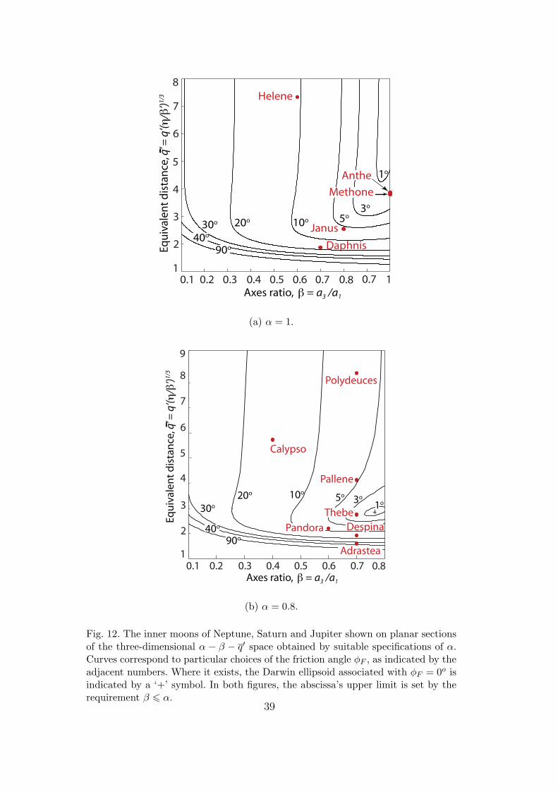
0.1 0.2 0.3 0.4 0.5 0.6 0.7Axes ratio, β = a3 /a1

1

2

3

4

5

6

7

8

0.8

Daphnis

Janus

Helene

40o

3o

5o

10o20o30o

90o

1o

Methone

AntheE

qu

iva

len

t d

ista

nce

, q’ =

q‘(η

/β’)

1/3

0.7 1

(a) α = 1.

Calypso

Polydeuces

0.1 0.2 0.3 0.4 0.5 0.6 0.7Axes ratio, β = a3 /a1

1

2

3

4

5

6

7

8

9

40o

3o5o10o20o

30o

90o

1o

Pallene

Pandora

0.8

Despina

Thebe

Adrastea

Eq

uiv

ale

nt

dis

tan

ce, q

’ = q

‘(η

/β’)

1/3

(b) α = 0.8.

Fig. 12. The inner moons of Neptune, Saturn and Jupiter shown on planar sectionsof the three-dimensional α − β − q′ space obtained by suitable specifications of α.Curves correspond to particular choices of the friction angle φF , as indicated by theadjacent numbers. Where it exists, the Darwin ellipsoid associated with φF = 0o isindicated by a ‘+’ symbol. In both figures, the abscissa’s upper limit is set by therequirement β 6 α.

39

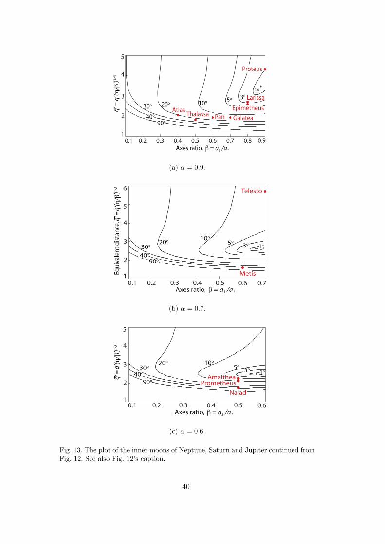
0.90.1 0.2 0.3 0.4 0.5 0.6 0.7 0.8Axes ratio, β = a3 /a1

1

2

3

4

5

ThalassaGalatea

1o

40o

3o

5o

10o20o

30o

90o

Proteus

Larissa

PanAtlas Epimetheusq

’ = q

‘(η

/β’)

1/3

(a) α = 0.9.

0.70.1 0.2 0.3 0.4 0.51

2

3

4

Axes ratio, β = a3 /a1

5

0.6

Metis

1o

40o

3o5o10o

20o

30o

90o

Equ

ival

ent

dis

tan

ce, q

’ = q

‘(η/β

’)1/3 6 Telesto

(b) α = 0.7.

0.60.1 0.2 0.3 0.4 0.51

2

3

4

Axes ratio, β = a3 /a1

5

1o

40o3o5o

10o20o

30o

90oPrometheus

Amalthea

Naiad

q’ =

q‘(η

/β’)

1/3

(c) α = 0.6.

Fig. 13. The plot of the inner moons of Neptune, Saturn and Jupiter continued fromFig. 12. See also Fig. 12’s caption.

40

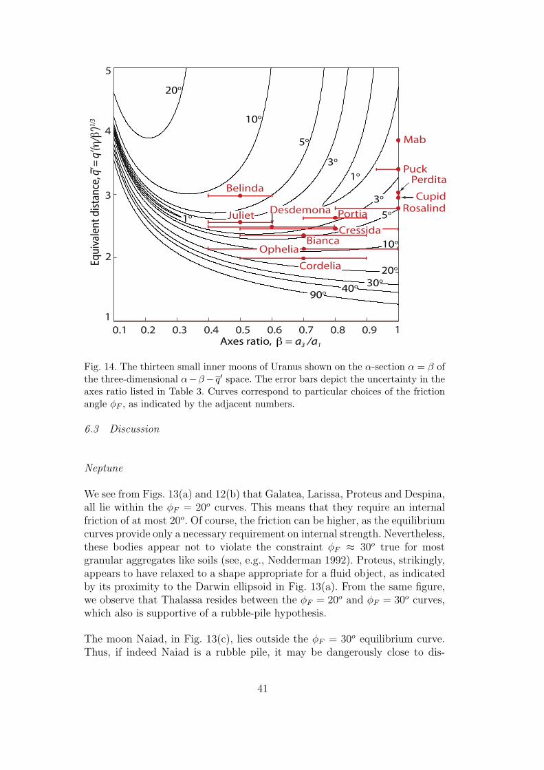
CupidRosalind

Puck

Belinda

0.1 0.2 0.3 0.4 0.5 0.6 0.7 0.8 0.9 1Axes ratio, β = a3 /a1

1

2

3

4

5

1o

5o

10o

20o

5o

90o

30o

10o

1o

3o

40o

20o

Mab

Perdita

Cordelia

Juliet PortiaDesdemona

BiancaCressida

3o

Ophelia

Equ

ival

ent

dis

tan

ce, q

’ = q

‘(η/β

’)1/3

Fig. 14. The thirteen small inner moons of Uranus shown on the α-section α = β ofthe three-dimensional α−β− q′ space. The error bars depict the uncertainty in theaxes ratio listed in Table 3. Curves correspond to particular choices of the frictionangle φF , as indicated by the adjacent numbers.

6.3 Discussion

Neptune

We see from Figs. 13(a) and 12(b) that Galatea, Larissa, Proteus and Despina,all lie within the φF = 20o curves. This means that they require an internalfriction of at most 20o. Of course, the friction can be higher, as the equilibriumcurves provide only a necessary requirement on internal strength. Nevertheless,these bodies appear not to violate the constraint φF ≈ 30o true for mostgranular aggregates like soils (see, e.g., Nedderman 1992). Proteus, strikingly,appears to have relaxed to a shape appropriate for a fluid object, as indicatedby its proximity to the Darwin ellipsoid in Fig. 13(a). From the same figure,we observe that Thalassa resides between the φF = 20o and φF = 30o curves,which also is supportive of a rubble-pile hypothesis.

The moon Naiad, in Fig. 13(c), lies outside the φF = 30o equilibrium curve.Thus, if indeed Naiad is a rubble pile, it may be dangerously close to dis-

41

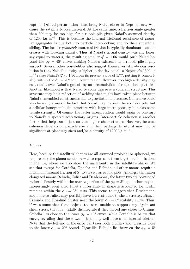
ruption. Orbital perturbations that bring Naiad closer to Neptune may wellcause the satellite to lose material. At the same time, a friction angle greaterthan 30o may be too high for a rubble-pile given Naiad’s assumed densityof 1200 kg m−3. This is because the internal frictional resistance of granu-lar aggregates is due both to particle inter-locking and to their superficialsliding. The former geometric source of friction is typically dominant, but de-creases with lowering density. Thus, if Naiad’s actual density was any lower,say equal to water’s, the resulting smaller q′ = 1.66 would push Naiad be-yond the φF = 40o curve, making Naiad’s existence as a rubble pile highlysuspect. Several other possibilities also suggest themselves. An obvious reso-lution is that Naiad’s density is higher; a density equal to Neptune’s 1600 kgm−3 raises Naiad’s q′ to 1.96 from its present value of 1.77, putting it comfort-ably within the φF = 20o equilibrium region. However, too high a density maycast doubt over Naiad’s genesis by an accumulation of ring/debris particles.Another likelihood is that Naiad to some degree is a coherent structure. Thisstructure may be a reflection of welding that might have taken place betweenNaiad’s assembled constituents due to gravitational pressure. Coherence couldalso be a signature of the fact that Naiad may not even be a rubble pile, buta cellular honeycomb-like structure with large micro-porosity but also sometensile strength. Of course, the latter interpretation would again be contraryto Naiad’s suspected accretionary origins. Inter-particle cohesion is anotherfactor that helps an object sustain higher shear stresses. However, becausecohesion depends on particle size and their packing density, it may not besignificant at planetary sizes and/or a density of 1200 kg m−3.

Uranus

Here, because the satellites’ shapes are all assumed proloidal or spherical, werequire only the planar section α = β to represent them together. This is donein Fig. 14, where we also show the uncertainty in the satellite’s shape. Wesee that except for Cordelia, Ophelia and Belinda, all other moons require amaximum internal friction of 5o to survive as rubble piles. Amongst the ratherelongated moons Belinda, Juliet and Desdemona, the latter two are positionedrather delicately within the narrow portion of the φF = 3o equilibrium region.Interestingly, even after Juliet’s uncertainty in shape is accounted for, it stillremains within the φF = 3o limits. This seems to suggest that Desdemona,and more so Juliet, may possibly have low resistance to shear stresses. Bianca,Cressida and Rosalind cluster near the lower φF = 5o stability curve. Thus,if we assume that these objects too were unable to support any significantshear stress, they may tidally disintegrate if they moved any closer to Uranus.Ophelia lies close to the lower φF = 10o curve, while Cordelia is below thatcurve, revealing that these two objects may well have some internal friction.Note that the left end of the error bar takes both Ophelia and Cressida closeto the lower φF = 20o bound. Cigar-like Belinda lies between the φF = 5o

42

and φF = 10o curves. Spread in its location due shape uncertainties stillkeep it within this region. Finally, if Belinda’s density were about 1900 kgm−3 rather than the assumed 1270 kg m−3, Belinda would require enoughfrictional strength to prevent gravitational collapse. Recall that crossing theupper bounding curve represents inability of the body to sustain its internalgravity. For a more careful analysis of Uranus’ moons, much more informationabout their shapes and densities would be required.

Saturn

From Figs. 12 and 13 we observe that all of Saturn’s inner moons fall within theequilibrium curves corresponding to a friction angle of 20o. This is encouraging,as it supports the hypothesis that these low-density objects formed throughan accretion of ring particles around an initial seed mass (Porco et al. 2007).Atlas, Pan and Daphnis appear to be the only satellites that have utilized theirincreased internal shear resistance to explore equilibrium regions accessibleto rubble piles. In fact, other than Atlas, Pan, Calypso and Daphnis, theremaining ten moons all lie inside the φF = 10o curve. This lack of spreadcould suggest weak internal friction in Saturn’s moons correlated, perhaps, totheir low densities; cf. our discussion on Naiad above.

It is instructive to note that if we neglected Saturn’s oblateness, Prometheus inFig. 13(c), in keeping with behavior noted in Fig. 6, would lie well outside theφF = 10o curve. Similarly, Atlas in Fig. 13(a) would be outside the φF = 20o

equilibrium region, not within.

Jupiter

Thebe in Fig. 12(b) lies within the φF = 3o equilibrium curve, very close tothe shape achieved by a fluid ellipsoid at equilibrium, though this does notnecessarily imply that Thebe’s interior is fluid-like in nature. Amalthea, witha calculated density of 857 kg m−3, is shown in Fig. 13(c) to require materialwith an internal friction angle slightly more than 5o to support itself. Thiscontributes to the hypothesis that this low-density satellite of Jupiter may infact be a granular aggregate. In fact, at Amalthea’s low density, we do noteexpect it to satisfy high frictional requirements.

Fig. 12(b) shows Adrastea to fall between the φF = 30o and φF = 40o equi-librium limits. This is very similar to the Neptunian Naiad in Fig. 13(c),except that Adrastea’s assumed density is much lower than Naiad’s. Becausethe equilibrium curves for the higher friction angles bunch up at higher axesratios β, slight errors in the satellite’s density can drastically influence inter-nal structure hypotheses. Thus, if we allowed for an error of about ±10% inAdrastea’s assumed density, we would obtain either 900 kg m−3 or 750 kg m−3

43

as its density. The former density would yield a q′ ≈ 1.64, locating Adrasteaon the φF = 30o equilibrium curve, thereby lending some support to any pro-posed rubble-pile model. However, 30o may yet be too high a friction anglenotwithstanding Adrastea’s suggested higher density of 900 kg m−3, and thisindicates that Adrastea’s density is even greater. In contrast, the lower den-sity of 750 kg m−3 is equivalent to a q′ of about 1.53 which pushes Adrasteaoutside the φF = 40o curve, and thereby makes Adrastea’s existence as an in-coherent, cohesion-less rubble pile extremely uncertain. Similar analyses maybe performed for errors in a satellite’s orbital radius q′, though these tend tobe much better constrained.

In Fig. 13(b), Metis lies beyond even the φF = 40o curve. Recalling that gran-ular aggregates, especially ones with Metis’ low density, seldom have frictionangles beyond 40o, this strongly suggests that Metis’ density is in fact higherthan its neighbors; recall that q′ ∼ ρ1/3. This would be in keeping with thepredictions of Thomas et al. (1998), who based on a study of craters on Metissuggested ρ = 1500 kg m−3. At this density, Metis’ q′ equals 1.92, placing itwell within the φF = 20o curve, a far more appropriate location for a granularMetis. There may also be present some degree of coherence and/or cellularstructure and/or inter-particle cohesion; cf., our discussion for Naiad above.Either this, or Metis is on the verge of failure.

7 Conclusions

In this paper, we have obtained general equations governing the equilibrium ofan ellipsoidal tidally-locked rubble-pile satellite of an ellipsoidal primary. Thisconstituted an extension of the first Darwin problem to the case of granularaggregates. The general formulation was then specialized to the case of ellip-soidal satellites of oblate primaries to investigate the equilibrium of the smallinner moons of the giant planets. In addition, we derived a Roche limit suit-able for rubble piles in orbit about spherical primaries, and applied it to Mars’moons. We also made contact with the earlier results of Davidsson (2001), andwere able to provide a more rigorous rationale for their correctness.

Several immediate avenues of exploration are now available. The first, morestraightforward one, is to apply the results in this paper to asteroidal satellites.The second, more involved problem is to investigate the equilibrium of binaries,i.e., systems where both the primary and the satellite are gravitational heldgranular aggregates of comparable mass. It will also be interesting to explorethe dynamical passage into equilibrium of such rubble-pile satellites. As in thecase of rubble piles in pure spin, this exercise, apart from providing insight intothe accretionary process that formed/shape them, is helpful for comparisonswith (as yet unavailable) n-body simulations of these granular systems.

44

8 Acknowledgements

I thank Sivasambu Mahesh of Indian Institute of Technology Kanpur, AnindyaChatterjee of Indian Institute of Science, Bangalore, and Joe Burns and JimJenkins of Theoretical and Applied Mechanics, Cornell University for helpfuldiscussions. I also thank Anthony Dobrovolskis of Lick Observatory, U. C.Santa Cruz and Dan Scheeres of Colorado University for insightful reviewsthat have made this work better.

References

Abramowitz, M., and I. A. Stegun 1965. Handbook of Mathematical Functions.New York: Dover.

Aggarwal, H. R., and V. R. Oberbeck 1974. Roche limit of a solid body.Astrophys. J. 191, 577–588.

Anderson, J. D., and 11 others 2005. Amalthea’s density is less than that ofwater. Science 308, 1291–1293.

Ashenberg, J. 2005. Proposed method for modeling the gravitational interac-tion between finite bodies. J. Guid. Control Dynam. 28, 768–774.

Banfield, D., and N. Murray 1992. A dynamical history of the inner Neptuniansatellites. Icarus 99, 390–401.

Belytschko, T., W. L. Liu, and B. Moran 2000. Nonlinear Finite Elements forContinua and Structures. NY: John Wiley and Sons.

Burns, J. A. 1992. Contradictory clues as to the origin of the Martian moons.In H. H. Kieffer, B. M. Jakosky, C. W. Snyder, and M. S. Matthews (Eds.),Mars, pp. 1283–1301. Tucson, AZ: U. Arizona Press.

Burns, J. A., I. Sharma, and J. T. Jenkins 2007. Approximate equilibriumshapes for spinning, gravitating rubble asteroids. BAAS 39, 50.07.

Burns, J. A., D. P. Simonelli, M. R. Showalter, D. P. Hamilton, C. C. Porco,L. W. Esposito, and H. Throop 2004. Jupiter’s ring-moon system. InF. Bagenal and T. Dowling (Eds.), Jupiter. The Planet, Satellites and Mag-netosphere, pp. 241–262. Cambridge, UK: Cambridge U. Press.

Chandrasekhar, S. 1969. Ellipsoidal Figures of Equilibrium. New Haven, CT:Yale Univ. Press.

Chen, W. F., and D. J. Han 1988. Plasticity for Structural Engineers. NewYork: Springer-Verlag.

Cooper, N. J., C. D. Murray, M. W. Evans, K. Beurle, R. A. Jacobson, andC. C. Porco 2008. Astrometry and dynamics of Anthe (S/2007 S 4), a newsatellite of Saturn. Icarus 195, 765–777.

Cooper, N. J., C. D. Murray, C. C. Porco, and J. N. Spitale 2006. CassiniISS astrometric observations of the inner Jovian satellites, Amalthea andThebe. Icarus 181, 223–234.

45

Darwin, G. 1906. On the figure and stability of a liquid satellite. Phil. Trans.R Soc. A 206, 161–248.

Davidsson, B. 1999. Tidal splitting and rotational breakup of solid spheres.Icarus 142, 525–535.

Davidsson, B. 2001. Tidal splitting and rotational breakup of solid biaxialellipsoids. Icarus 149, 375–383.

Dobrovolskis, A. R. 1982. Internal stresses in Phobos and other triaxial bodies.Icarus 52, 136–148.

Dobrovolskis, A. R. 1990. Tidal disruption of solid bodies. Icarus 88, 24–38.Duxbury, T. C., and J. D. Callahan 1989. Phobos and Deimos control net-

works. Icarus 77, 275–286.Fung, Y. C. 1965. Foundations of Solid Mechanics. Englewood Cliffs, NJ:

Prentice-Hall.Greenwood, D. T. 1988. Principles of Dynamics. Englewood Cliffs, NJ:

Prentice-Hall.Holsapple, K. A. 2001. Equilibrium configurations of solid cohesionless bodies.

Icarus 154, 432–448.Holsapple, K. A. 2008. Spinning rods, elliptical disks and solid ellipsoidal

bodies: Elastic and plastic stresses and limit spins. Int. J. Non-LinearMech., doi:10.1016/j.ijnonlinmec.2008.03.011.

Holsapple, K. A., and P. Michel 2006. Tidal disruptions: A continuum theoryfor solid bodies. Icarus 183, 331–348.

Holsapple, K. A., and P. Michel 2008. Tidal disruptions II. A continuumtheory for solid bodies with strength with applications to the Solar System.Icarus 193, 283–301.

Jacobson, R. A. 1998. The orbits of the inner Uranian satellites from Hubblespace telescope and Voyager 2 observations. AJ 115, 1195–1199.

Jacobson, R. A., and W. M. Owen, Jr. 2004. The orbits of the inner Nep-tunian satellites from Voyager, Earth-based, and Hubble Space Telescopeobservations. AJ 128, 1412–1417.

Jacobson, R. A., J. Spitale, C. C. Porco, K. Beurle, N. J. Cooper, M. W. Evans,and C. D. Murray 2008. Revised orbits of Saturn’s small inner satellites.AJ 135, 261–263.

Karkoschka, E. 2001. Voyager’s eleventh discovery of a satellite of Uranus andphotometry and the first size measurements of nine satellites. Icarus 151,69–77.

Karkoschka, E. 2003. Sizes, shapes, and albedos of the inner satellites ofNeptune. Icarus 162, 400–407.

Kinoshita, H. 1972. First-order perturbations of the two finite body problem.Publ. Astron. Soc. Japan 24, 423–457.

Knowles, J. K. 1998. Linear Vector Spaces and Cartesian Tensors. Oxford:Oxford U. Press.

Love, A. E. H. 1946. A Treatise on the Mathematical Theory of Elasticity (4thed.). New York: Dover.

Murray, C. D., and S. F. Dermott 1999. Solar System Dynamics. Cambridge:

46

Cambridge U. Press.Nedderman, R. M. 1992. Statics and Kinematics of Granular Materials. Cam-

bridge: Cambridge U. Press.Porco, C. C. 1991. An explanation of Neptune’s ring arcs. Science 400,

995–1001.Porco, C. C., and 35 others 2005. Cassini imaging science: Initial results on

Saturn’s rings and small satellites. Science 307, 1226–1236.Porco, C. C., P. C. Thomas, J. W. Weiss, and D. C. Richardson 2007. Saturn’s

small inner moons: Clues to their origins. Science 318, 1602–1607.Porco, C. C., J. W. Weiss, P. C. Thomas, D. C. Richardson, R. A. Jacobson,

and J. Spitale 2006. Physical characteristics and possible accretionary ori-gins for Saturn’s small satellites. In S. Mackwell and E. Stansbery (Eds.),37th Annual Lunar and Planetary Science Conference, Volume 37 of Lunarand Planetary Institute Conference Abstracts, pp. 2289–2289.

Richardson, D. C., P. Elankumaran, and R. E. Sanderson 2005. Numericalexperiments with rubble piles: Equilibrium shapes and spins. Icarus 173,349–361.

Roche, E. 1847. La figure d’une masse fluide soumise a l’attraction d’un pointeloigne. Acad. des Sci. de Montpellier 1, 243–262.

Schaeffer, D. G. 1987. Instability in the evolution equations describing incom-pressible granular flow. J. Diff. Equations 66, 19–50.

Scheeres, D. J. 2006. Relative equilibria for general gravity fields in the sphere-restricted full 2-body problem. Celest. Mech. Dyn. Astr. 94, 317–349.

Sharma, I. 2004. Rotational Dynamics of Deformable Ellipsoids with Applica-tions to Asteroids. Ph. D. thesis, Cornell University.

Sharma, I., J. T. Jenkins, and J. A. Burns 2005a. Equilibrium configurationsand the Roche limit for spinning ellipsoidal soil-like asteroids. BAAS 37,643.

Sharma, I., J. T. Jenkins, and J. A. Burns 2005b. Equilibrium shapes of ellip-soidal soil asteroids. In R. Garcıa-Rojo, H. J. Hermann, and S. McNamara(Eds.), Proceedings of the 5th International Conference on Micromechanicsof Granular Media, Volume 1, pp. 429–432. A. A. Balkema.

Sharma, I., J. T. Jenkins, and J. A. Burns 2006. Tidal encounters of ellipsoidalgranular asteroids with planets. Icarus 183, 312–330.

Sharma, I., J. T. Jenkins, and J. A. Burns 2008. Dynamical passage to approx-imate equilibrium shapes for spinning, gravitating rubble asteroids. Icarus ,In review.

Shor, V. A. 1975. The motion of the Martian satellites. Celest. Mech. Dyn.Astr. 12, 61–75.

Showalter, M. R., and J. J. Lissauer 2006. The second ring-moon system ofUranus: Discovery and dynamics. Science 311, 973–977.

Thomas, P. C., J. A. Burns, L. Rossier, D. Simonelli, J. Veverka, C. R. Chap-man, K. Klaasen, T. V. Johnson, and M. J. S. Belton 1998. The small innersatellites of Jupiter. Icarus 135, 360–371.

Thomas, P. C., C. Weitz, and J. Veverka 1989. Small satellites of Uranus:

47

Disk-integrated photometry and estimated radii. Icarus 81, 92–101.Truesdell, C., and R. A. Toupin 1960. The classical field theories. In S. Flugge

(Ed.), Encyclopedia of Physics Vol. III/I: Principles of classical mechanicsand field theory, pp. 226–793. Berlin: Springer-Verlag.

Werner, R. A., and D. J. Scheeres 2005. Mutual potential of homogeneouspolyhedra. Celest. Mech. Dyn. Astr. 91, 337–349.

A Cartesian tensors and coordinate systems

In this paper, we will need to employ two separate cartesian coordinate sys-tems, viz., the principal-axes coordinate systems attached to the primary andthe satellite that are defined by the unit vectors e′i and ei, respectively. Thesetwo coordinate systems are shown in Fig. 1, where they are denoted by P andS. The components of a vector a in P will be denoted by a′i and in S by ai,so that we have the identities

a = (a · e′i)e′i = a′ie′i = (a · ei)ei = aiei, (A.1)

where we have, and subsequently will employ, indical notation.

Because of the several possible relative orientations of P and S, we seek todevelop a coordinate-free representation. To this end, we utilize a tensor-basedapproach. A first-order tensor is simply a vector. A second-order tensor, say A,is the coordinate-independent counterpart of a matrix, so that A also operateson a vector to produce another vector. Third- and fourth-order tensors relatinglower-order tensors to other lower-order tensors may be similarly defined.

To better understand tensors, it is useful to generalize the concept of a unitvector to a tensorial basis. Such a generalization is furnished by the tensorproduct (a ⊗ b) of two vectors a and b. The entity a ⊗ b is a second-ordertensor that can act on another vector c in two different ways to yield anothervector:

(a⊗ b) · c = (c · b)a and c · (a⊗ b) = (c · a)b , (A.2)

where the ‘.’ on the left hand sides denotes a tensor operation, and the usualvector dot product on the right hand sides. The computation,

a⊗ b = aiei ⊗ bj ej = (aibj)ei ⊗ ej ⇐⇒ a′ie′i ⊗ b′j e′j = (a′ib

′j)e′i ⊗ e′j, (A.3)

suggests that a tensorial basis may be constructed by taking appropriate ordertensor products of the unit vectors. Thus, a second-order tensorial basis in theprimary’s coordinate system P is given by the nine quantities e′i⊗ e′j. Similarlywe have ei ⊗ ej in S. A second-order tensor A can then be written as

A = A′ij e′i ⊗ e′j = Aij ei ⊗ ej, (A.4)

48

in terms of A’s components Aij in P and A′ij in S, respectively. These com-ponents, obtained by appealing to (A.2), are given by the equations

A′ij = e′i ·A · e′j and Aij = ei ·A · ej, (A.5)

that are reminiscent of analogous ones for vector components; see (A.1). Wewill refer to the nine Aij’s (A′ij) as the “matrix of A in S (P )” denoted by[A] ([A]′). A second-order tensor’s interactions with vectors and other second-order tensors may be obtained by repeated (if required) application of (A.2).These operations are summarized below:

A · a = Aij ei ⊗ ej · amem = Aijaj ei (A.6a)

a ·A = amem · Aij ei ⊗ ej = aiAij ej, (A.6b)

A ·B = Aij ei ⊗ ej ·Bmnem ⊗ en = AijBjnei ⊗ en (A.6c)

and A : B = Aij ei ⊗ ej : Bmnem ⊗ en = Aij ei ·Bjnen = AijBji, (A.6d)

where the first two operations produce vectors, the next another second-ordertensor, and the third a scalar. The double-dot product (:), as its form suggests,denotes a sequential application of dot products. A’s actions on higher-ordertensors may be analogously defined. When there is no confusion, second-ordertensors are referred to simply as tensors.

The transpose (‘T’) and inverse (‘-1’) of a tensor A may be interpreted fromtheir corresponding matrix definitions

[AT ] = [A]T and [A−1] = [A]−1. (A.7)

If S is a symmetric tensor, i.e., ST = S , it is possible to find an orthogonalcoordinate system, say the e′i of P , in which S ’s matrix is diagonal, so thatwe may write

S =3∑i=1

S ′ie′i ⊗ e′i, (A.8)

where S ′i, the components of S in P are called the eigenvalues of S corre-sponding to S ’s eigenvectors e′i. Finally, to every vector w, there correspondsan anti-symmetric tensor W = −W T that is formed by the components of win any coordinate system, i.e.,

W = −εijkw′ie′j ⊗ e′k = −εijkwiej ⊗ ek, (A.9)

where εijk is the alternating third-order tensor (see below), such that εijk = 1or -1, if i 6= j 6= k form an even or an odd permutation, respectively, and 0otherwise.

In the sequel, we will need to find the components of vectors and second-ordertensors in one coordinate system, say S, given its matrix in the other, say P .

49

This may be done by expressing the unit vectors of P in terms of those of Sas,

e′i = (e′i · ej)ej,and substituting this relationship into the first of (A.1) and (A.5). Geometri-cally, because both P and S are right-handed Cartesian coordinate systems,it is possible to obtain one from the other by a rotation. A rotation, becauseit takes vectors to vectors, is a second-order tensor, and we write

e′i = T · ei,

in terms of the rotation tensor T = T ′ij e′i ⊗ e′j = Tij ei ⊗ ej. It may be shown

that, in fact,Tij = [T ]ij = T ′ij = [T ]′ij ≡ e′j · ei. (A.10)

Substituting the previous two equations into (A.1) and (A.5), we obtain thecoordinate transformation rules

[a] = [T T · a]′ = [T ]T [a]′ ⇐⇒ ai = Tjia′j (A.11a)

and [A] = [T T ·A ·T ]′ = [T ]T [A]′[T ]⇐⇒ Aij = TkiA′klTlj (A.11b)

for vector and second-order tensor components, respectively.

Next, consider third-order tensors. In terms of the third-order tensorial bases,e′i ⊗ e′j ⊗ e′k in P and ei ⊗ ej ⊗ ek in S, a third-order tensor is defined as

A = A′ijke′i ⊗ e′j ⊗ e′k = Aijkei ⊗ ej ⊗ ek, (A.12)

so that A′ijk and Aijk are the components in P and S, respectively. The actionsof A on vectors and other tensors of various orders are defined in a mannersimilar to that of a second-order tensor (A.6), e.g.,

A · a = Aijkei ⊗ ej ⊗ ek · amem = Aijkakei ⊗ ej (A.13a)

and a ·A = amem · Aijkei ⊗ ej ⊗ ek = aiAijkej ⊗ ek. (A.13b)

Fourth-order tensors are formed in a manner analogous to third-order tensors,

A = A′ijkle′i ⊗ e′j ⊗ e′k ⊗ e′l = Aijklei ⊗ ej ⊗ ek ⊗ el, (A.14)

and their operations on vectors and tensors of various orders may be developedby following (A.6) and (A.13), for example,

A : B = Aijklei ⊗ ej ⊗ ek ⊗ el : Bmnem ⊗ en = AijklBlkei ⊗ ej. (A.15)

50