UNIVERSITY OF NOTTINGHAM

SCHOOL OF ECONOMICS

DISCUSSION PAPER NO. 98/21

The Endowment Effect and Expected Utility

by

Gwendolyn C. Morrison

Abstract

The endowment effect, which is well documented in the contingent valuationliterature, alters people’s preferences according to a reference point established in theelicitation question. Experimental results from the literature and from a study intothe value of non-fatal road injuries are shown to be evidence that an endowment effectis also at work in standard gambles.

AcknowledgementsSome results discussed in this paper are from a study undertaken in 1991 for the UKDepartment of Transport and Transport Research Laboratory (see Jones-Lee et al1995).

2

1. Introduction

Evidence has amassed supporting the existence of an endowment effect (or

status quo bias) in contingent valuation studies (Thaler, 1980). The endowment effect

is a reference point effect usually attributed to loss aversion (Kahneman and Tversky,

1979). Willingness to pay questions ask people to give up some money to acquire

(more of) a good and willingness to accept questions ask them to give up (some of) a

good in exchange for some money. As presented in Morrison (1998) the endowment

effect can be incorporated in a utility function: U=f($, X, loss). That is, the utility

that people place on a bundle is both a positive function of the quantities of the goods

comprising the bundle, and a negative function of any loss (real or hypothetical) that

the elicitation question asks them to incur. If an individual is asked to choose

between two bundles, neither of which they own, then they have nothing to lose and

the utility they ascribe to the bundles is simply a function of the goods in each. But,

most preference elicitation methods used by economists require people to express

their preferences for one good (bundle) in terms of their willingness to forego some of

another good. Consequently, it is reasonable to expect that, and prudent to check

whether, an endowment effect is also evident in other methods of preference

elicitation such as von Neumann-Morgenstern’s standard gambles.

2. Background

The endowment effect was offered as an explanation for the disparity

frequently found between willingness to pay (WTP) and willingness to accept (WTA)

measures of value (e.g., Knetsch and Sinden, 1984 & 1987; Knetsch, 1989). This

disparity has persisted even when controlling for assorted other possible sources of

divergence including income effects (e.g., Brookshire et al, 1987; McDaniels, 1992),

3

Hanemann’s (1991) substitutability argument (e.g., Bateman et al, 1997; Morrison,

1997a), learning (Coursey et al, 1987), incentives (using choice experiments (eg.,

Kahneman et al, 1990; Franciosi et al, 1996) and using Vickrey auctions (e.g.,

Coursey et al, 1987)), trophy effects (by using exchange goods (e.g., van Dijk et al,

1996)), and imprecise preferences (e.g., Dubourg et al, 1994 &1997; Morrison, 1998).

Shogren et al’s (1994) study is the only one that rejected an endowment effect in

consumption goods (they rejected the endowment effect in favour of Hanemann’s

argument), but Morrison (1997b) showed that their results do no preclude the

presence of an endowment effect.

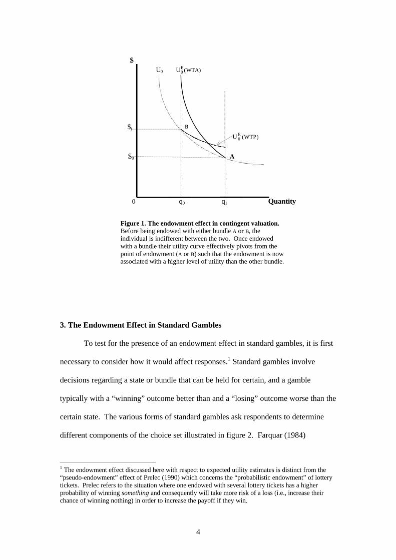
Morrison 1997b illustrated this effect with a pivot of the indifference curve

from the point of endowment, as in figure 1. This pivot effectively increases the level

of utility associated with the endowment. In contingent valuation studies, the

endowment effect manifests itself in people having to be paid more to give up a good

once they own it than they would be willing to pay to acquire the good in the first

place. That is, their willingness to accept exceeds their willingness to pay. If the point

of endowment alters peoples’ preferences such as illustrated in Morrison (1997b),

then this may have serious implications for all preference elicitation techniques since

the point of endowment is an, often arbitrary, component of the survey questions

used. If an endowment effect is evident in other elicitation methods, then it is

important that care is taken in choosing the endowments used in questionnaires so as

not to introduce unnecessary and arbitrary bias into the results of economic

evaluations.

4

$ U0 U0

E WTA( )

1$ B

U 0E WTP( )

$0 A

0 q0 q1 Quantity

Figure 1. The endowment effect in contingent valuation.Before being endowed with either bundle A or B, theindividual is indifferent between the two. Once endowedwith a bundle their utility curve effectively pivots from thepoint of endowment (A or B) such that the endowment is nowassociated with a higher level of utility than the other bundle.

3. The Endowment Effect in Standard Gambles

To test for the presence of an endowment effect in standard gambles, it is first

necessary to consider how it would affect responses.1 Standard gambles involve

decisions regarding a state or bundle that can be held for certain, and a gamble

typically with a “winning” outcome better than and a “losing” outcome worse than the

certain state. The various forms of standard gambles ask respondents to determine

different components of the choice set illustrated in figure 2. Farquar (1984)

1 The endowment effect discussed here with respect to expected utility estimates is distinct from the“pseudo-endowment” effect of Prelec (1990) which concerns the “probabilistic endowment” of lotterytickets. Prelec refers to the situation where one endowed with several lottery tickets has a higherprobability of winning something and consequently will take more risk of a loss (i.e., increase theirchance of winning nothing) in order to increase the payoff if they win.

5

describes the four different formulations of standard gamble questions. Only the

Probability Equivalent and Certainty Equivalent forms of question are examined here

because the relevant empirical evidence is restricted to these.

First consider the case of probability equivalence questions. Probability

equivalence (PE) questions endow a respondent with a bundle that they can have for

certain, and asks the respondent to choose the probability that makes them indifferent

between the certain bundle and the gamble. This decision is illustrated in figure 2

with x being the certain state, W and L being the winning and losing pay-outs of the

lottery respectively, and p being the probability of winning.

Choose between

(1-p) (W)

(x)win

for certain p (L)

lose

Figure 2. Standard gamble questions. The objective of all forms of SG questions is to find a certainstate and a gamble that are associated with the same level of utility. Typically, the winning payout, W,exceeds the amount that can be held for certain, x, which in turn exceeds the payout associated withlosing the gamble, L. Respondents are asked to determine one component of the decision problem (x,p, L, or W) such that it makes them indifferent between having the certain state or the gamble—that is,such that (x) ~ (p, L; (1- p), W).

An endowment effect essentially increases the utility of an owned good

relative to alternative goods. So, if an endowment effect is at work, then once

endowed with x that individual will require a better gamble (i.e., one with a higher

expected value) in order to be persuaded to swap their endowment, x, for the gamble.

So they will reject some gambles that they would have chosen over x had they not

6

been endowed with x. Figures 3(a) and 3(b) illustrate PE and CE responses relative to

a fair gamble, respectively. Each point on the 45º line (certainty line) represents a

gamble for which the outcome associated with winning is the same as for losing.

Points above the certainty line are irrelevant because they represent gambles for

which the winning outcome is worse than the losing outcome.

First consider a PE question that endows an individual with x for certain

(figure 3a). The starting point of the question (i.e., the endowment) corresponds to

point A on the certainty line. The response (i.e., choice of gamble) is illustrated by a

ray from the starting point, A, to a point below the certainty line. A ray from point A

to the horizontal axis represents a gamble for which the “lose” outcome is the

“lowest” outcome considered in the analysis. This can be greater than, equal to, or

less than zero. Ray AN is the locus of fair gambles—the iso-expected value line. Any

response with an expected value of less than (more than) $X indicates a risk seeker

(risk averter). For clarity, consider a risk neutral individual. Given the choice

between $X for certain and a gamble with an expected value of $X, they will be

indifferent between the two. So they should be willing to swap their $X for any

gamble along the ray AN. However, since an endowment effect increases the utility

of an owned good relative to alternatives, it would lead the respondent to reject all of

the fair gambles. They would require a gamble with an expected value greater than

$X (i.e., a gamble to the right of line segment AN). This would be misinterpreted to

mean that our risk neutral individual is risk averse. The same rationale applies to

individuals with other risk attitudes. They would reject gambles that they would have

accepted had they not been endowed with x, thus implying a higher degree of risk

aversion than is the case.

7

Lose

Certainty Line

x A

RS RA 45°

L x N Win

Figure 3(a). PE responses in relation to a fairgamble.

Lose

Certainty Line

N'

RA RS 45°

L A' Win

Figure 3(b). CE responses in relation to a fairgamble

All gambles on the certainty line have the same payoff for a win as for a loss. Payoffs associated with‘winning’ a gamble are measured on the horizontal axis, and those associated with a loss are measuredalong the vertical axis. The starting point (i.e., the endowment) for the PE question is point A infigure 3(a), while the starting point for a CE question is illustrated as point A' on the horizontal axis.Line segments AN and A'N' are the iso-expected value (iso-EV) lines. All points along this linerepresent gambles with probabilities of winning and losing such that their expected value is equal to x.Therefore a risk neutral individual will be indifferent between any gamble along this line.

Conversely, CE questions endow people with a gamble and then ask them to

indicate the certainty equivalent of the gamble. That is, the values of p, W, and L in

figure 2 are given, and the respondent is asked to assign a value to the certain state (x)

that would make them indifferent between keeping the gamble and trading it for x.

Where point A' represents the starting point for a CE question in figure 3(b), the ray

A'N' is the iso-expected value line and, so, depicts a risk neutral response. An

endowment effect increases the utility of an owned good relative to other available

goods, and in this case the endowment is a gamble. Therefore, respondents will

require a higher certainty equivalent as compensation for giving up the gamble with

which they were endowed. In this case our risk neutral individual would state a CE

indicating that they are risk seeking or, a risk averse individual would appear less risk

averse than they really are.

8

3.1 The endowment effect and the PE-CE disparity

From this we can form predictions of the over-all pattern of standard gamble

responses in the presence of an endowment effect: one for paired PE and CE

questions, and one for chained standard gamble questions. First consider the situation

in which the same individuals are asked to answer “mirrored” PE and CE questions.

The questions are “mirrored” in that the response to one question serves as a fixed

starting point for the other. If an endowment effect is the driving force behind the PE-

CE disparity, then within subject comparisons of PE and CE responses should reveal

that people are relatively more risk averse in their PE responses than in their CE

responses. If an endowment effect is the sole or main source of inconsistency in

standard gambles, then this relationship should hold regardless of which form of

question was asked first and regardless of whether the questions are in the gain or loss

domain.

Results obtained by Hershey et al (1982 & 1985) fit in with the endowment

effect predictions for both CE and PE questions. Hershey et al (1982) found that

between subject experiments revealed different risk attitudes for the same gamble

depending on whether it was presented as a PE or CE question. In particular,

responses to CE questions exhibit more risk seeking than PE responses (they found

this to be significant at p<.01). This result would be stronger if within subject

comparisons were considered. Hershey et al (1985) did so using four groups of

respondents and asking four paired PE-CE questions of each.

Figure 4(a) depicts the pattern of within subject inconsistency they observed

between mirror image PE and CE responses where the PE questions were asked first.

The representative PE responses are illustrated by the movement from point A on the

certainty line to point B on the horizontal axis (the dotted ray). This movement is to

9

the right of ray AN, the risk neutral line, as it is a risk averse response. The

corresponding representative CE response is shown by the movement from point B to

a point such as C back on the certainty line (the solid ray). Since the CE response is

less risk averse, but not risk seeking, point C must lie somewhere between points A

and D. (The implications of Hershey et al’s (1985) results for the Healthy Years

Equivalent measure of health (Gafni et al, 1991) which uses both PE and CE

questions to obtain a single measure of an individual’s state of health are discussed in

Morrison (1997c).) Similarly, figure 4(b) illustrates the pattern of responses when the

CE question was asked first. The representative CE response is risk seeking (hence

the ray A'B' is to the right of the line indicating risk neutrality, A'N') and the

response to the mirror image PE question is more risk averse.

Lose

Certainty Line

D

A C

isoEV

isoEV

L N B Win

Figure 4(a). PE question asked first.1) PE: Risk Averse; 2) CE: less Risk Averse. The thick lines illustrate risk neutral responses.The average response to the PE question isshown by the movement from point A to pointB, and the follow-up CE average response bythe movement from point B to a point such as C.Since the CE responses tended to be risk aversebut less risk averse than the PE responses pointC will lie on the certainty line between points Aand D. A CE response to the right of linesegment BD would indicate risk seekingbehaviour.

Lose

Certainty Line

B'

N' isoEV

isoEV

L A' C' D' C' Win

Figure 4(b). CE question asked first.1) CE: Risk Seeking; 2) PE: more Risk Averse. The thick lines illustrate risk neutral responses.The average response to the CE question isshown by the movement from point A' to pointB', and the follow-up PE average response by themovement from point B' to point C'. Since thePE responses tended to be more risk averse thanthe CE questions, C' will be to the right of A' onthe horizontal axis. If the PE response is (morerisk averse but) still risk seeking, then C' will liebetween A' and D'. If the PE response exhibitsrisk aversion, then C' will lie to the right of D'.

10

The mapping of the utility functions elicited from respondents that are less risk

averse in their CE responses than in their PE responses will correspond to figure 5. In

this figure the value function is held to be the same with respect to the PE and CE

responses and it is assumed that the observed pattern of inconsistency holds for all

values of the good. It shows that when endowed with a certain state (as in a PE

question) an individual will attach a higher utility to that state than if they had instead

been endowed with a gamble (as in a CE question). This has been termed the utility

evaluation effect (Machina, 1989).

Expected Utility, Value

V(max)=EU(max) (chained PE)

PE

Measurable Value Function

CE (unchained PE)

V(min)=EU(min)

min X max Good

Figure 5. The Utility Evaluation Effect:utility functions elicited from PE and CE questionsand from chained and unchained PE questions

Setting the value function relevant to the PE and CE questions to beequal, the expected utility functions arising from these two methods willbe different. PE responses tended to be more risk averse than CEresponses. This suggests that when endowed with a certain state or good,as in the PE questions, an individual places a higher utility on that certaingood than if they had instead been endowed with a gamble. Similarly, theutility functions arising from chained and unchained PE questions will bedifferent.

To summarise, in the gain domain and in the loss domain, those asked CE

questions first were relatively more risk averse in their PE responses, and those asked

PE questions first were relatively less risk averse in their CE responses. As Hershey

11

et al (1985) conclude, “This means that for both gains and losses, the PE-CE subjects

were relatively less risk-averse in the CE mode. This pattern holds true for all

questions, being statistically significant (p<.05) for 14 out of 16 cases under an exact

binomial test for asymmetry” (p. 1222). Although those authors briefly address the

endowment effect as a possible source of the disparity, they reject it stating that,

“According to this explanation, a subject would overestimate the adjustment needed

to make the two options equally attractive, because the preferred option is seen as

more attractive once owned…The net effects correspond neither in magnitude nor in

pattern to the empirical data” (p.1228). The endowment effect attaches a premium to

the owned option—if they own a gamble then they require a better certainty

equivalent to give it up, and if they own the certain state they require a better gamble

(here a probability equivalent) to part with that. This is what Hershey et al’s (1985)

results showed for 14 of the 16 cases, with the remaining two cases being skewed in

the anticipated direction but not statistically significant. The pattern observed in

responses, is that predicted for the presence of an endowment effect.

So, just as the endowment effect results in willingness to accept (WTA)

exceeding willingness to pay (WTP), it also results in EU estimates from PE questions

exceeding those obtained from CE questions. That is, the upward (downward) bias on

WTA (WTP) responses and the upward (downward) bias on PE (CE) responses,

imposed by an endowment effect, is a source of the WTP-WTA and PE-CE disparity.

3.2 The endowment effect and chained gambles

Next, consider chained gambles. Chained gambles combine responses to two

or more PE questions to obtain one expected utility estimate (other forms of standard

gamble questions could be used, but this author is only aware of PE questions being

12

chained). The independence axiom of expected utility dictates that changing the

outcomes used in the gamble should not change the utility elicited. Therefore,

chained and unchained gambles should yield equal EU estimates. However, as

previously noted, an endowment effect will lead individuals to give PE responses that

suggest they are more risk averse than they really are. If an endowment effect is

present in PE responses, then it would be present in both (all) stages of the chained

gamble. So we would expect an endowment effect to suggest a higher degree of risk

aversion than is the case, and we would expect that effect to be compounded across

every stage of the chained gamble. Consequently, in the presence of an endowment

effect, the pattern of responses that we would expect to emerge is that EU estimates

from chained gambles should exceed those from a single gamble.

PE questions are frequently used to quantify health states to estimate health

gains from treatments or health lost through injuries (Torrance, 1986; Hornberger et

al, 1992; Stiggelbout et al, 1994; Jones-Lee et al, 1995; Jansen et al, 1998).

Typically, respondents are asked to state the probability of success or failure (winning

or losing) that would make them indifferent between remaining in a (generally

hypothetical) state of ill health and accepting a risky treatment that could improve or

could worsen that state of health. In this context if the EU of a health state, X, is

estimated using a PE question, then the endowment effect in effectively making the

individual more risk averse will increase the estimated EU of state X. That is, state X

would appear to be closer to ‘full’ or ‘normal’ health. And if a chained gamble is

used, then the endowment effect would be compounded across the gambles leading to

the chained gamble estimate exceeding the unchained estimate.

Indeed, this is the pattern that emerges (e.g., Llewellyn-Thomas et al, 1982;

Rutten-van Mölken et al, 1995; Bleichrodt, 1996; Morrison, 1996). Chained and

13

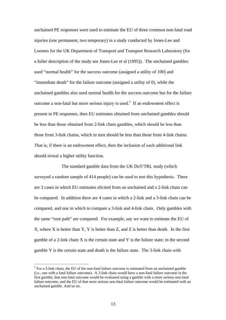
unchained PE responses were used to estimate the EU of three common non-fatal road

injuries (one permanent, two temporary) in a study conducted by Jones-Lee and

Loomes for the UK Department of Transport and Transport Research Laboratory (for

a fuller description of the study see Jones-Lee et al (1995)). The unchained gambles

used “normal health” for the success outcome (assigned a utility of 100) and

“immediate death” for the failure outcome (assigned a utility of 0), while the

unchained gambles also used normal health for the success outcome but for the failure

outcome a non-fatal but more serious injury is used.2 If an endowment effect is

present in PE responses, then EU estimates obtained from unchained gambles should

be less than those obtained from 2-link chain gambles, which should be less than

those from 3-link chains, which in turn should be less than those from 4-link chains.

That is, if there is an endowment effect, then the inclusion of each additional link

should reveal a higher utility function.

The standard gamble data from the UK DoT/TRL study (which

surveyed a random sample of 414 people) can be used to test this hypothesis. There

are 3 cases in which EU estimates elicited from an unchained and a 2-link chain can

be compared. In addition there are 4 cases in which a 2-link and a 3-link chain can be

compared, and one in which to compare a 3-link and 4-link chain. Only gambles with

the same “root path” are compared. For example, say we want to estimate the EU of

X, where X is better than Y, Y is better than Z, and Z is better than death. In the first

gamble of a 2-link chain X is the certain state and Y is the failure state; in the second

gamble Y is the certain state and death is the failure state. The 3-link chain with

2 For a 2-link chain, the EU of the non-fatal failure outcome is estimated from an unchained gamble(i.e., one with a fatal failure outcome). A 3-link chain would have a non-fatal failure outcome in thefirst gamble, that non-fatal outcome would be evaluated using a gamble with a more serious non-fatalfailure outcome, and the EU of that more serious non-fatal failure outcome would be estimated with anunchained gamble. And so on.

14

which it is compared has the same first gamble, the second gamble has Y as the

certain state and Z as the failure state, and finally the third gamble has Z as the certain

state and death as the failure state. Table 1 presents the results of within subject pair-

wise tests investigating the hypothesis that the greater the number of links in a chain

the greater the estimated EU. A non-parametric test is used because individuals

indicated their responses on an answer sheet with a payment scale—this may have

effected the distribution of responses. Specifically, one-tailed Wilcoxon matched-

pairs signed-ranks tests were used to test the null that the number of links in a chain

does not affect the estimated EU against the alternative that a chain with (m+1) links

would obtain an EU estimate exceeding that from a chain with only m links. In all

eight cases, the null that the two estimates are equal has to be rejected (at α=.05) in

favour of the alternative that the addition of a link increases the estimated EU. In fact

in seven of those cases, the null is rejected at the 1% level of significance. These

results are consistent with the presence of an endowment effect.

Unchained vs 2-link chainPattern of Responses Wilcoxon mean (std dev)

m+1 > m = m+1 < m 1-tailed m m+1case 1 210 146 35 p < .01 84.6 (21.8) 93.9 (13.0)case 2 86 258 55 p < .01 94.1 (16.8) 96.2 (10.6)case 3 79 253 64 p < .01 94.1 (16.8) 97.1 (8.8)

2-link vs 3-link chaincase 4 113 259 25 p < .01 96.2 (10.6) 98.0 (6.8)case 5 52 313 30 p < .05 98.4 (7.0) 98.7 (5.5)case 6 51 317 27 p < .01 98.4 (7.0) 99.1 (4.7)case 7 74 315 7 p < .01 97.4 (9.7) 98.6 (6.9)

3-link vs 4-link chaincase 8 70 314 10 p < .01 98.7 (5.5) 99.3 (4.0)

Table 1. Comparison of m-link and (m+1)-link chains.Case 1 concerns a permanent injury, while the rest concern temporary injuries.In comparing unchained and a 2-link chain, m refers to the unchained and (m+1) to the 2-link chain;for a comparison of 2- and 3-link chains, m refers to the 2-link and (m+1) to the 3-link; and so on.p values are for 1-tailed Wilcoxon matched-pairs signed-ranks tests.

15

These results indicate that using different failure outcomes in gambles will

recover different utility functions as in figure 5. Each link added to a chain reveals a

higher (implying more risk averse) utility function. This is the same as McCord and

de Neufville’s (1983) finding that different utility functions are retrieved when

different probability distributions are used with the certainty equivalent method—

higher levels of probability associated with the best outcome yield higher levels of

utility. This has been termed the “utility evaluation effect.”

The results in table 1 suggest that an endowment effect results in utility

estimates of health states being biased upward. This presents a problem for policy

making. If the purpose of obtaining EU estimates is to measure health gained from a

treatment or health loss prevented by new safety measures, then—given that an

endowment effect effectively pushes the estimates of all health states up toward “full”

health—estimated benefits of such programmes will be biased downward. Thus, an

endowment effect in PE responses that is not accommodated could lead to some types

of health care or safety measures being incorrectly rejected as being too costly relative

to the health gained or injuries prevented. This problem is likely to be exacerbated if

chained PE questions are used.

The notion of an endowment effect in standard gamble questions is similar in

some respects to Gafni and Torrance’s (1984) “gambling effect.” Gafni et al (1984)

propose that people are afraid of gambling per se and therefore require a risk premium

to compensate for having a gamble rather than a certain state. But such a ‘gambling

effect’ in probability equivalence responses would lead risk neutral people to choose a

certain state over a gamble, even when answering a CE question. This combined with

the acceptance that people are generally risk averse with respect to health and money,

illustrates that the ‘gambling effect’ is inconsistent with responses obtained by

16

Hershey et al (1985) when they presented people with CE questions first (i.e., they

were risk seeking). (The same must be said of Wakker et al’s (1995) argument that

inconsistencies in SG are predicted by Rank-dependent utility). However, both the

PE-CE disparity and the internal inconsistency in chained PE questions do conform

with predictions for the presence of an endowment effect.

Conclusion

Biases such as the endowment effect and embedding have received much

attention in the contingent valuation literature and has lead some to reject that method

as a means of quantifying costs and benefits in favour of other methods of preference

elicitation such as standard gambles (e.g., Jones-Lee et al, 1995). However, internal

inconsistencies in the standard gamble method that have been noted in the economics

literature have been shown here to conform to Thaler’s notion of an endowment

effect. Both the PE-CE disparity and the frequent observation that chained EU

estimates exceed the corresponding unchained estimates are predicted by the presence

of an endowment effect. EU has already taken a battering in the literature, hence the

emergence of the many non-EU models, however a series of experiments conducted

Hey and Orme (1994) found that the best model of responses is EU plus white noise.

Expected utility is the common model for decision making under uncertainty, and

standard gambles are the standard approach to obtaining EU estimates. The evidence

presented here is not intended as an additional argument against EU (and hence the

use of standard gambles), but rather as a warning and as a starting point for removing

bias from EU estimates. That is, if an endowment effect is present in standard gamble

responses, then care must be taken to accommodate this effect when interpreting

results for the purposes of policy making.

17

Identifying the presence of an inconsistency is the first step to understanding,

estimating, and accommodating that inconsistency. The evidence presented here is at

least sufficient to identify the presence of and the direction of a bias in standard

gambles and to show that this bias is, at least prima facie, of the same nature as the

endowment effect found in contingent valuation experiments. Since both contingent

valuation and standard gambles have been used to evaluate health and health care in

recent years, it is important that we ensure that biases present in one method are not

present in the other before using such biases as evidence of one method’s superiority.

18

References

Bateman, I.; Munro, A.; Rhodes, B.; Starmer, C.; and Sugden, R. (1997), “A test of the theory ofreference-dependent preferences”, Quarterly Journal of Economics, 112(2), 479-505.

Bleichrodt, H. (1996), “Applications of utility theory in the economic evaluation of health care”,Ph.D. thesis, Erasmus University Rotterdam.

Brookshire, D.S. and Coursey, D.L. (1987), “Measuring the value of a public good: an empiricalcomparison of elicitation procedures”, American Economic Review, 77(4), 554-566.

Coursey, D.L.; Hovis, J.L.; and Schulze, W.D. (1987), “The disparity between willingness to acceptand willingness to pay measures of value”, Quarterly Journal of Economics, 102, 679-690.

Dolan, P.; Jones-Lee, M. ; and Loomes, G. (1995), “Risk-risk versus standard gamble procedures formeasuring health state utilities”, Applied Economics, 27, 1103-1111.

Dubourg, W.R.; Jones-Lee, M.W.; and Loomes, G. (1994), “Imprecise preferences and the WTP-WTAdisparity”, Journal of Risk and Uncertainty, 9, 115-133.

Dubourg, W.R.; Jones-Lee, M.W.; and Loomes, G. (1997), “Imprecise preferences and survey design in contingent valuation”, Economica, 64, 681-702.

Farquhar, P.H. (1984), “Utility Assessment Methods”, Management Science, 30, 123-130.Franciosi, R.; Kujal, P.; Michelitsch, R.; Smith, V.; and Deng, G. (1996), “Experimental tests of the

endowment effect”, Journal of Economic Behavior and Organization, 30, 213-226.Gafni, A. and Torrance, G.W. (1984), “Risk attitude and time preference in health”, Management

Science, 30(4), 440-451.Hanemann, W.M. (1991), “Willingness to pay and willingness to accept: how much can they differ?”

American Economic Review, 81(3), 635-647.Hey, J.D. and Orme, C. (1994), “Investigating generalizations of Expected Utility theory using

experimental data”, Econometrica, 62(6), 1291-1326.Hornberger, J.C.; Redelmeier, D.A.; and Petersen, J. (1992), “Variability among methods to assess

patients’ well-being and consequent effect on a cost-effectiveness analysis”, Journal ofClinical Epidemiology, 45(5), 505-512.

Jansen, S.J.T.; Stiggelbout, A.M.; Wakker, P.P.; Vliet vlieland, T.P.M.; Leer, J.H.; and Nooy, M.A.;Kievit, J. (1998), “Patient utilities for cancer treatments: a study on the chained procedure forthe standard gamble and time trade-off”, Medical Decision Making, (in press).

Jones-Lee, M.W.; Loomes, G.; and Philips, P.R. (1995), “Valuing the prevention of non-fatal roadinjuries: contingent valuation vs standard gambles”, Oxford Economic Papers, 47, 676-695.

Kahneman, D.; Knetsch, J.L.; and Thaler, R.H. (1990), “Experimental tests of the endowment effectand the coase theorem”, Journal of Political Economy, 98(6), 1325-1348.

Kahneman, D. and Tversky, A. (1979), “Prospect theory: an analysis of decision under risk”,Econometrica, 47(2), 263-291.

Knetsch, J.L. (1989), “The endowment effect and evidence of non-reversible indifference curves”,American Economic Review, 79(5), 1277-1284.

Knetsch, J.L. and Sinden, J.A. (1984), “Willingness to pay and compensation demanded: experimentalevidence of an unexpected disparity in measures of value”, Quarterly Journal of Economics,99(3), 507-521.

Knetsch, J.L. and Sinden, J.A. (1987), “The persistence of evaluation disparities”, Quarterly Journal ofEconomics, 102, 691-695.

Llewellyn-Thomas, H.; Sutherland, H.J.; Tibshirani, R.; Ciampi, A.; Till, J.E.; Boyd, N.F. (1982), “Themeasurement of patients’ values in medicine”, Medical Decision Making, 2, 449-462.

Machina, M.J. (1989), “Choice under Uncertainty: problems solved and unsolved,” in J. Hey (ed.)Current Issues in Microeconomics, (Basingstoke: Macmillan).

McCord, M. and de Neufville, R. (1983), “Empirical demonstration that Expected Utility decisionanalysis is not operational”, in B.P. Stigum et al (eds.) Foundations of Utility and Risk Theorywith Applications (Dordrecht: D.Reidel Publishing Ltd).

McDaniels, T.L. (1992), “Reference points, loss aversion, and contingent values for auto safety”,Journal of Risk and Uncertainty, 5, 187-200.

Mehrez, A. and Gafni, A. (1991), “The Healthy-years Equivalents: how to measure them using thestandard gamble approach”, Medical Decision Making, 11, 140-146.

Morrison, G.C. (1996), “An Assessment and Comparison of Selected Methods for Eliciting Quality ofLife Valuations from the Public”, D.Phil. Thesis, University of York, UK.

Morrison, G.C. (1997a), “Willingness to pay and willingness to accept: some evidence of anendowment effect”, Applied Economics, 29, 411-417.

Morrison, G.C. (1997b), “Resolving differences in willingness to pay and willingness to accept:comment”, American Economic Review, 87(1), 236-240.

19

Morrison, G.C. (1997c), “HYE and TTO: what is the difference?” Journal of Health Economics, 16(5),563-578.

Morrison, G.C. (1998), “Understanding the disparity between WTP and WTA: endowment effect,substitutability, or imprecise preferences?” Economics Letters, 59(2), 189-194.

Prelec, D. (1990), “A ‘Pseudo-endowment’ Effect, and its Implications for Some Recent NonexpectedUtility Models”, Journal of Risk and Uncertainty, 3, 247-259.

Rutten-van Mölken, M.P.M.H.; Bakker, C.H.; van Doorslaer, E.K.A.; and van der Linden, S. (1995),“Methodological issues of patient utility measurement: experience from two clinical trials”,Medical Care, 33(9), 922-937.

Shogren, J.F.; Shin, S.Y.; Hayes, D.J.; and Kliebenstein, J.B. (1994), “Resolving differences inwillingness to pay and willingness to accept”, American Economic Review, 84(1), 255-270.

Stiggelbout, A.M.; Kiebert, G.M.; Kievit, J.; Leer, J.W.H.; Stoter, G.; de Haes, J.C.J.M. (1994),“Utility assessment in cancer patients: Adjustment of time tradeoff scores for the utility of lifeyears and comparison with standard gamble scores”, Medical Decision Making, 14, 82-90.

Thaler, R. (1980), “Toward a Positive Theory of Consumer Choice”, Journal of Economic Behaviorand Organization, 1, 39-60.

Torrance, G.W. (1986), “Measurement of health state utilities for economic appraisal: a review”,Journal of Health Economics, 5, 1-30.

van Dijk, E. and van Knippenberg, D. (1996), “Buying and selling exchange goods: Loss aversion andthe endowment effect”, Journal of Economic Psychology, 17, 517-524.

Wakker, P. and Stiggelbout, A. (1995), “Explaining distortions in Utility Elicitation through the Rank-dependent Model for Risky Choices”, Medical Decision Making, 15, 180-186.

20

$ U0 U0

E WTA( )

1$ B

U 0E WTP( )

$0 A

0 q0 q1 Quantity

Figure 1. The endowment effect in contingent valuation.Before being endowed with either bundle A or B, theindividual is indifferent between the two. Once endowedwith a bundle their utility curve effectively pivots from thepoint of endowment (A or B) such that the endowment is nowassociated with a higher level of utility than the other bundle.

21

Choose between

(1-p) (W)

(x)win

for certain p (L)

lose

Figure 2. Standard gamble questions. The objective of all forms of SG questions is to find a certainstate and a gamble that are associated with the same level of utility. Typically, the winning payout, W,exceeds the amount that can be held for certain, x, which in turn exceeds the payout associated withlosing the gamble, L. Respondents are asked to determine one component of the decision problem (x,p, L, or W) such that it makes them indifferent between having the certain state or the gamble—that is,such that (x) ~ (p, L; (1- p), W).

22

Lose

Certainty Line

x A

RS RA 45°

L x N Win

Figure 3(a). PE responses in relation to a fairgamble.

Lose

Certainty Line

N'

RA RS 45°

L A' Win

Figure 3(b). CE responses in relation to a fairgamble

All gambles on the certainty line have the same payoff for a win as for a loss. Payoffs associated with‘winning’ a gamble are measured on the horizontal axis, and those associated with a loss are measuredalong the vertical axis. The starting point (i.e., the endowment) for the PE question is point A infigure 3(a), while the starting point for a CE question is illustrated as point A' on the horizontal axis.Line segments AN and A'N' are the iso-expected value (iso-EV) lines. All points along this linerepresent gambles with probabilities of winning and losing such that their expected value is equal to x.Therefore a risk neutral individual will be indifferent between any gamble along this line.

23

Lose

Certainty Line

D

A C

isoEV

isoEV

L N B Win

Figure 4(a). PE question asked first.1) PE: Risk Averse; 2) CE: less Risk Averse. The thick lines illustrate risk neutral responses.The average response to the PE question isshown by the movement from point A to pointB, and the follow-up CE average response bythe movement from point B to a point such as C.Since the CE responses tended to be risk aversebut less risk averse than the PE responses pointC will lie on the certainty line between points Aand D. A CE response to the right of linesegment BD would indicate risk seekingbehaviour.

Lose

Certainty Line

B'

N' isoEV

isoEV

L A' C' D' C' Win

Figure 4(b). CE question asked first.1) CE: Risk Seeking; 2) PE: more Risk Averse. The thick lines illustrate risk neutral responses.The average response to the CE question isshown by the movement from point A' to pointB', and the follow-up PE average response by themovement from point B' to point C'. Since thePE responses tended to be more risk averse thanthe CE questions, C' will be to the right of A' onthe horizontal axis. If the PE response is (morerisk averse but) still risk seeking, then C' will liebetween A' and D'. If the PE response exhibitsrisk aversion, then C' will lie to the right of D'.

24

Expected Utility, Value

V(max)=EU(max) (chained PE)

PE

Measurable Value Function

CE (unchained PE)

V(min)=EU(min)

min X max Good

Figure 5. The Utility Evaluation Effect:utility functions elicited from PE and CE questionsand from chained and unchained PE questions

Setting the value function relevant to the PE and CE questions to beequal, the expected utility functions arising from these two methods willbe different. PE responses tended to be more risk averse than CEresponses. This suggests that when endowed with a certain state or good,as in the PE questions, an individual places a higher utility on that certaingood than if they had instead been endowed with a gamble. Similarly, theutility functions arising from chained and unchained PE questions will bedifferent.

25

Unchained vs 2-link chainPattern of Responses Wilcoxon mean (std dev)

m+1 > m = m+1 < m 1-tailed m m+1case 1 210 146 35 p < .01 84.6 (21.8) 93.9 (13.0)case 2 86 258 55 p < .01 94.1 (16.8) 96.2 (10.6)case 3 79 253 64 p < .01 94.1 (16.8) 97.1 (8.8)

2-link vs 3-link chaincase 4 113 259 25 p < .01 96.2 (10.6) 98.0 (6.8)case 5 52 313 30 p < .05 98.4 (7.0) 98.7 (5.5)case 6 51 317 27 p < .01 98.4 (7.0) 99.1 (4.7)case 7 74 315 7 p < .01 97.4 (9.7) 98.6 (6.9)

3-link vs 4-link chaincase 8 70 314 10 p < .01 98.7 (5.5) 99.3 (4.0)

Table 1. Comparison of m-link and (m+1)-link chains.Case 1 concerns a permanent injury, while the rest concern temporary injuries.In comparing unchained and a 2-link chain, m refers to the unchained and (m+1) to the 2-link chain;for a comparison of 2- and 3-link chains, m refers to the 2-link and (m+1) to the 3-link; and so on.p values are for 1-tailed Wilcoxon matched-pairs signed-ranks tests.

26