the electrical conductivity of the oceanic upper...

Geophys. J . Int. (1992) 110, 159-179

The electrical conductivity of the oceanic upper mantle

Graham Heinson’.* and Steven Constable2 ‘Research School of Earth Sciences, Australian National University, Canberra, ACT 2601, Australia ‘Scripps Institution of Oceanography, La Jolla, CA 92093, USA

Accepted 1992 January 23. Received 1992 January 20; in original form 1991 April 18

SUMMARY Previous inversions of sea-floor magnetotelluric (MT) sounding data have predicted upper mantle electrical conductivities which are more than an order of magnitude higher than laboratory measurements of the conductivity of olivine would suggest, and controlled source-field electromagnetic (CSEM) soundings require a lithospheric mantle conductivity of 3 x lop5 Sm-’, which is so low that the electromagnetic (EM) coast effect would produce more anisotropy in MT soundings than is observed. We address these issues by constructing an olivine mantle model for conductivity and examining the inversion of MT data from three sea-floor sites, and show that the incompatibilities can be largely resolved if the effects of oceans and coastlines are considered. Our mantle model is based on recent measurements of olivine conductivity, the conductivity of tholeiite melt, a thermal model for the upper mantle based on lithospheric cooling and the temperature of a+ a + /3 olivine transition, the pyrolite model of mantle petrology, and conductivities derived from CSEM sounding. We propose Archie’s Law with exponent 2 and interconnected tubes as realistic lower and upper bounds for the effect of partial melt on rock conductivity, and Archie’s Law with exponent 1.5 as the preferred estimate. The 1-D forward response of this model is not compatible with observed sea-floor MT data. Three data sets presented by Oldenburg (1981) pass a test for one-dimensionality based on the size of the residuals when fit with Parker’s D+ algorithm, but two of the three soundings fail a test for independence of residuals. We also find that the presence of the upper mantle ‘high-conductivity zone’ previously inferred from these data is highly dependent on data misfit and not required when the misfit criterion is relaxed a reasonable amount. Re-inversions of the MT data produce models which are incompatible with our petrological model of mantle conductivity. However, by adding an ocean with various coastlines of simple geometry to our petrological model and solving the forward 3-D problem using thin-sheet analysis we predict MT responses which are distorted in a manner that is remarkably similar to the observed data.

Key words: electrical conductivity, oceanic upper mantle, 1-D inversion, sea-floor magnetotellurics, thin-sheet 3-D modelling.

INTRODUCTION

The electrical conductivity of mantle materials depends on temperature, mineralogy and fluid content, and so conductivity is an important parameter in the study of the thermal and structural evolution of oceanic lithosphere. There are three sources of information on the conductivity of the oceanic upper mantle: (1) measurements of the

Now at: School of Earth Sciences, Flinders University, Adelaide, SA 5042. Australia.

conductivity of mantle materials made in the laboratory; (2) MT soundings made on the sea-floor using Earth’s natural magnetic field as a source; and (3) EM soundings made on the sea-floor using a controlled source-field. In this paper we attempt to establish the extent to which results from all three methods are consistent. On first inspection there is little agreement; laboratory measurements of olivine conductivity imply that the conductivities inferred from the MT studies require very high temperatures or large fractions of partial melt, and the very resistive uppermost mantle

159

160 G. Heinson and S . Constable

inferred from CSEM experiments would suggest an extremely persistent coast effect which would produce more anisotropy in MT soundings than is generally observed. We do not wish to review all this literature and will cite the relevant work as we proceed through the analysis. The reader is referred to a recent review by Constable (1990).

Our paper is presented in three sections. In the first section, we review laboratory measurements on olivine, the major constituent of the upper mantle, as well as petrological and thermal models of the oceanic mantle, and use these to make predictions of temperature, melt fraction and upper mantle electrical conductivity as a function of depth and age. In the second section, we take three typical sea-floor MT soundings and examine them carefully using modern 1-D inversion techniques to find realistic models of conductivity structure. Finally, we use a thin-sheet modelling algorithm to quantify the level of distortion on the MT fields that would be expected in an ocean basin whose lithospheric conductivity is determined by the laboratory and CSEM studies.

1 PREDICTIONS FROM LABORATORY DATA

1.1 Introduction

Estimates of upper mantle conductivity based on laboratory data are important in the interpretation of electrical soundings for three reasons.

First, in the ideal case where the conductivity structure of the upper mantle can be determined uniquely from EM sounding data, the laboratory data can be used to infer the physical properties of the upper mantle, such as temperature and melt fraction. In the more realistic case, bounds on conductivity can be converted to bounds on physical properties.

The second reason arises from the non-uniqueness of the EM inversion problem. The decisions as to what models are geologically realistic are often carried out in an ad hoc manner. For example, 1-D inversion of MT data may result in conductivity structures which are entirely consistent with the observations, but which are geologically unlikely, such as the discrete finite conductance delta functions of Parker's (1980) D+ model. Few researchers would accept this as a geologically reasonable model of Earth, yet are less critical in accepting the output from other modelling schemes. Apart from providing an indication of the geological feasibility of models generated to fit sounding data, the inclusion of laboratory information can be used to reduce the non-uniqueness of the problem. For example, in a marine CSEM sounding, Cox et al. (1986) constrained mantle conductivity below 20 km depth using laboratory measurements of olivine conductivity in order to obtain better resolution above 20 km.

Finally, EM sounding data can be used to test the hypotheses generated by the laboratory experiments. That is, the EM response of conductivity models derived from laboratory data may be tested for compatibility with the sounding data. Alternatively, a class of inversion methods exists which generates the model closest to the a priori

model and which is compatible with the data (e.g. Parker, Shure & Hildebrand 1987).

Before we investigate these ideas, we first need to determine realistic models of electrical conductivity structure of oceanic upper mantle, independently of MT sounding data, by using laboratory conductivity data and other geophysical and petrological information. Unfortun- ately, the uncertainty in the range of petrological models is large. We will argue that the different models of chemical composition of the upper mantle are not a major factor in determining the conductivity structure. Of far greater importance is the presence of a region of partial melt or volatiles which has been used to explain the seismic low-velocity zone/electrical high-conductivity zone (Olden- burg 1981; Sato, Selwyn-Sacks & Murase 1989). Most geothermal models of the oceanic lithosphere (e.g. Parson & Sclater 1977) are shown to be consistent with a region of partial melt, where the width and depth of the zone are a function of age of the oceanic lithosphere, but the fraction of partial melt is less well-constrained.

1.2 Geothermal models

The construction of suitable geotherms for Earth is not straightfoxward, as Earth's thermal structure is poorly understood. In this analysis, simple modelling procedures are used, dividing the upper mantle into a non-viscous thermal lithosphere in which the dominant mode of heat-flow is conduction, and a convective region extending beneath the thermal lithosphere into Earth.

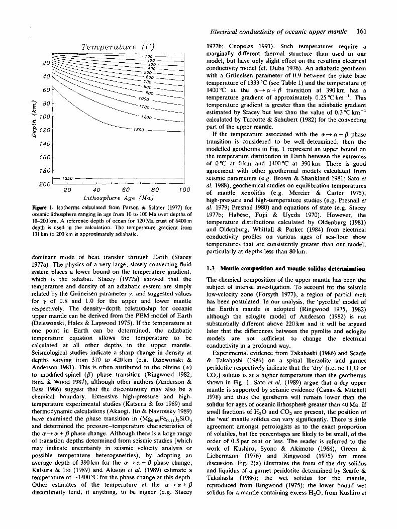
Simple models of a cooling half-space (Parker & Oldenburg 1973) and rigid plate (McKenzie 1967; Parson & Sclater 1977) have been advanced to explain the approximately linear relationship between the ocean depth and the square root of age, for sea-floor ages up to 100Ma (Marty & Cazenave 1989). For older sea-floor, the depth and the heat-flow observations appear to decay exponen- tially to constant values. Parson & Sclater (1977) show that the cooling plate model is consistent with bathymetry and to a lesser extent heat-flow data for a wide range of sea-floor ages; their analysis permits an inversion of bathymetry to give the model parameters of plate thickness, temperature at the base of the plate and thermal expansion coefficient. Comparison of these parameters for the north Pacific and the north Atlantic agree within experimental uncertainties (Table 1) and we choose to use Pacific values simply because the MT soundings discussed later are from this region. The temperature distribution in the lithospheric plate may be calculated using a 1-D heat-flow approximation (Parson & Sclater 1977; equation 29) for ages of oceanic lithosphere ranging from 10 to 100 Ma, as shown in Fig. 1.

Beneath the thermal lithosphere, convection is the

Table 1. Plate model parameters determined by Parson & Sclater (1977) for the North Pacific and the North Atlantic.

Plate Thickness Plate Base Thermal Expansion

(km) Temp. ( " c ) Coefficient ( " C - ' )

1333 ? 274 (3.28 f 1.19) X 10.'

1365 f 276 (3.10 f 1.11) X 10.'

North Pacific 125 f 10

North Atlantic 128 ? 10

Electrical conductivity of oceanic upper mantle 161

1977b; Chopelas 1991). Such temperatures require a marginally different thermal structure than used in our model, but have only slight effect on the resulting electrical conductivity model (cf. Duba 1976). An adiabatic geotherm with a Griineisen parameter of 0.9 between the plate base temperature of 1333 "C (see Table 1) and the temperature of 1400°C at the a+a+/3 transition at 390km has a temperature gradient of approximately 0.25 "C km-'. This temperature gradient is greater than the adiabatic gradient estimated by Stacey but less than the value of 0.3"Ckm-' calculated by Turcotte & Schubert (1982) for the convecting part of the upper mantle.

If the temperature associated with the a+ (Y + /3 phase transition is considered to be well-determined, then the modelled geotherms in Fig. 1 represent an upper bound on the temperature distribution in Earth between the extremes of 0°C at 0 km and 1400 "C at 390 km. There is good agreement with other geothermal models calculated from seismic parameters (e.g. Brown & Shankland 1981; Sat0 et al. 1988), geochemical studies on equilibration temperatures of mantle xenoliths (e.g. Mercier & Carter 1975), high-pressure and high-temperature studies (e.g. Presnall et al. 1979; Presnall 1980) and equations of state (e.g. Stacey 1977b; Habese, Fujii & Uyeda 1970). However, the temperature distributions calculated by Oldenburg (1981) and Oldenburg, Whittall & Parker (1984) from electrical conductivity profiles on various ages of sea-floor show temperatures that are consistently greater than our model, particularly at depths less than 80 km.

140

160

180

Tempera ture (C)

-

-

- 1350

200 20 40 60 80 100

Lithosphere A g e (Ma) Figvre 1. Isotherms calculated from Parson & Sclater (1977) for oceanic lithosphere ranging in age from 10 to 100 Ma over depths of 10-200 km. A reference depth of ocean for 120 Ma crust of 6400 m depth is used in the calculation. The temperature gradient from 131 km to 200 km is approximately adiabatic.

dominant mode of heat transfer through Earth (Stacey 1977a). The physics of a very large, slowly convecting fluid system places a lower bound on the temperature gradient, which is the adiabat. Stacey (1977a) showed that the temperature and density of an adiabatic system are simply related by the Griineisen parameter y, and suggested values for y of 0.8 and 1.0 for the upper and lower mantle respectively. The density-depth relationship for oceanic upper mantle can be derived from the PEM model of Earth (Dziewonski, Hales & Lapwood 1975). If the temperature at one point in Earth can be determined, the adiabatic temperature equation allows the temperature to be calculated at all other depths in the upper mantle. Seismological studies indicate a sharp change in density at depths varying from 370 to 420km (e.g. Dziewonski & Anderson 1981). This is often attributed to the olivine (a) to modified-spinel (@) phase transition (Ringwood 1982; Bina & Wood 1987), although other authors (Anderson & Bass 1986) suggest that the discontinuity may also be a chemical boundary. Extensive high-pressure and high- temperature experimental studies (Katsura & Ito 1989) and thermodynamic calculations (Akaogi, Ito & Navrotsky 1989) have examined the phase transition in (M~,,,Fe,~,,),SiO, and determined the pressure-temperature characteristics of the a+ a + B phase change. Although there is a large range of transition depths determined from seismic studies (which may indicate uncertainty in seismic velocity analysis or possible temperature heterogeneities), by adopting an average depth of 390 km for the a+ a + /3 phase change, Katsura & Ito (1989) and Akaogi et af. (1989) estimate a temperature of -1400 "C for the phase change at this depth. Other estimates of the temperature at the a--*cr+@ discontinuity tend, if anything, to be higher (e.g. Stacey

1.3 Mantle composition and mantle solidus determination

The chemical composition of the upper mantle has been the subject of intense investigation. To account for the seismic low-velocity zone (Forsyth 1977), a region of partial melt has been postulated. In our analysis, the 'pyrolite' model of the Earth's mantle is adopted (Ringwood 1975, 1982) although the eclogite model of Anderson (1982) is not substantially different above 220 km and it will be argued later that the differences between the pyrolite and eclogite models are not sufficient to change the electrical conductivity in a profound way.

Experimental evidence from Takahashi (1986) and Scarfe & Takahashi (1986) on a spinal lherzolite and garnet peridotite respectively indicate that the 'dry' (i.e. no H,O or CO,) solidus is at a higher temperature than the geotherms shown in Fig. 1. Sat0 et al. (1989) argue that a dry upper mantle is supported by seismic evidence (Canas & Mitchell 1978) and thus the geotherm will remain lower than the solidus for ages of oceanic lithosphere greater than 40 Ma. If small fractions of H,O and CO, are present, the position of the 'wet' mantle solidus can vary significantly. There is little agreement amongst petrologists as to the exact proportion of volatiles, but the percentages are likely to be small, of the order of 0.5per cent or less. The reader is referred to the work of Kushiro, Syono & Akimoto (1968), Green & Liebermann (1976) and Ringwood (1975) for more discussion. Fig. 2(a) illustrates the form of the dry solidus and liquidus of a garnet peridotite determined by Scarfe & Takahashi (1986); the wet solidus for the mantle, reproduced from Ringwood (1975); the lower bound wet solidus for a mantle containing excess H,O, from Kushiro et

162 G. Heinson and S. Constable

(a) Upper Mantle So l idus Curves I 2000

1800

I

L t,

1600 3 u t

2 1400

1200

1 OOG

Scarfe k Takahashz (1986) _ -

40 80 120 160 200 Depth ( k m )

Pyrolite So l idus a n d Melt Fractzon Curves (b)

1400

1350

1300

1250

I t,

9,

!i 2 1200

2

r-

1150

1100

1050

1000 40 80 120 160 200

Depth (km)

Fiyre 2. (a) The 'dry' mantle solidus curve of a garnet peridodite (Scarfe & Takahashi 1986) and the 'wet' solidus curve for a pyrolite mantle (Ringwood 1975) used in this paper to calculate the melt fraction and distribution. Also shown are the 'wet' solidus curve for a C0,-saturated mantle (Wyllie 1977) and the 'wet' solidus curve for an H,O-saturated mantle (Kushiro er al. 1968) which represents a lower bound of temperature for the onset of melting in the mantle. Solidus curves (dashed lines) are superimposed on geotherms (solid lines) from Fig. 1 for lithosphere 10-100 Ma. (b) The mantle solidus curve for the onset of melting of a pyrolite mantle (light dashed line) and percentages of melt as a function of temperature and depth (heavy dashed lines) estimated by Ringwood (1975). The percentage melt curves and the solidus are superimposed on geotherms (solid lines) from Fig. 1 for lithosphere 10-100 Ma.

al. (1%8); and the pure C0,-saturated mantle solidus from Wyllie (1977), superimposed on the mantle geotherms shown in Fig. 1. Ringwood (1975) argues for 0.1 per cent H,O with an uncertainty factor of 2; this wet solidus is used in our model for the important reason that partial melt fractions are also given as a function of pressure and temperature. Fig. 2(b) shows the wet solidus of Ringwood (1975) and the percentage of partial melt as a function of temperature and depth, with the geotherms from Fig. 1.

Figure 2(b) shows the intersection of the geotherms with Ringwood's mantle solidus at depths of 40-90 km for oceanic lithosphere age 10-100 Ma, thus generating a small percentage of melt. The eclogite model of Anderson (1982) differs little from the pyrolite model over the low-velocity zone, and incipient melting is again used to explain seismic attenuation. The presence of partial melt in the upper mantle has long been advanced as an explanation of the seismic low-velocity zone (Forsyth 1977), but other mechanisms have also been proposed. For example, Liu (1989) argues that the low-velocity zone results from a fraction of free H,O between the water line at a depth of 250 km and the stability field of amphibole in the oceanic upper mantle. Another alternative hypothesis by Green & Gueguen (1974) attributes seismic attenuation to bubbles of a C0,-rich fluid phase. Recently, Karato (1990) has proposed that hydrogen ions dissolved in the olivine lattice may increase the plasticity of the asthenosphere by a factor of 1.5-3 to account for the observed low seismic velocities.

If the melt curves for a 0.1 per cent H,O mantle shown in Fig. 2(a) and (b) are representative of the partial melt distribution, then the width of the partial melt zone is compatible with calculations of seismic attenuation (Leeds, Knopoff & Kausel 1974; Forsyth 1977). Fig. 3 illustrates the percentages of partial melt calculated from Fig. 2(b) as a function of age and depth. From this simple analysis, it appears that the peak percentage of partial melt varies both in magnitude and depth with different ages of oceanic lithosphere. Seismic evidence (Canas & Mitchell 1978) and

M e l t F r a c t i o n (%)

40

60

7 80

100 Y

;s 9 : T ' l 180

200:- ' I 20 40 60 80 100

Lzthosphere Age (Ma) Figure 3. Percentages of partial melt obtained in Fig. 2(b) from the intersection of the geothcrms with the pyrolite mantle solidus.

Electrical conductiviu of oceanic upper mantle 163

San Carlos olivine conductivities are considered a reliable model for the upper mantle.

If the pyrolite model of upper mantle is adopted, then petrological estimates of the percentage of olivine range from 78 per cent for the residual harzburgite layer (6-30 km depth), 65 per cent for the residual lherzolite layer (30-40 km), and 57 per cent for the depleted pyrolite down to the L Y - + C U + ~ discontinuity (Ringwood 1982). The principal accompanying minerals are orthopyroxene with smaller proportions of clinopyroxene and garnet. A higher proportion of olivine has been proposed by Bina & Wood (1987), who argue that an upper mantle containing 70 per cent olivine is required to satisfy P and S wave velocities at the L Y - + c u + / ~ discontinuity. The eclogite model of Anderson (1982) is not substantially different from the pyrolite model to a depth of 220km. Below 220km, Anderson argues that eclogite must be present to satisfy seismic and free-Earth oscillation observations. D u e & Anderson (1989) calculate percentages of olivine in the eclogite model to be 40 per cent in the upper mantle, with 37 per cent clinopyroxene, 13 per cent garnet and 10 per cent orthopyroxene. The percentages of garnet and clinopyroxene in the eclogite layer are much higher than at corresponding depths in the pyrolite upper mantle.

Little is known of the electrical conductivity properties of upper mantle minerals other than for olivine. Measurements made by Duba, Boland & Ringwood (1973) on an orthopyroxene suggested that the conductivity was perhaps an order of magnitude less than that of olivine. Direct measurements on garnet are not available. Some measurements of a garnet peridotite have been made (Rai & Manghnani 1978) but these samples were crushed and sintered, a process which invariably seems to increase conductivity. It is unclear whether associated minerals will increase or decrease the conductivity of a perfect olivine mantle. However, Constable et al. (1992) demonstrate a remarkable agreement between the conductivities of a lherzolite xenolith and S02, so that the purely olivine basis for our mantle model does not appear to be a problem.

Seismic velocity analysis suggests that the upper mantle is anisotropic, with a deformation-induced lattice preferred orientation of olivine concentrating in the direction of flow (Ribe 1989). The preferred orientation is parallel to the [100] axis, which is intermediate in conductivity between the directions of maximum ([001]) and minimum ([OlO]) conductivity. We therefore do not expect a strong conductivity signature from the anisotropy in olivine orientation in the upper mantle due to thermally activated conduction. However, we note that the mechanism proposed by Karato (1990) to enhance conductivity in the asthenosphere by allowing the passage of hydrogen ions through the olivine lattice in the (1001 axis, will produce significant anisotropy in conductivity.

The implications of melt in the upper mantle are discussed below, but since models of mantle petrology exclude volatiles (Sato et af. 1988), and consequently involve no melt fraction away from the ridge-axis, we can present a model of mantle conductivity based entirely on the geothermal model in Fig. 1 and the conductivity- temperature relationship for SO2 in equation (1). Fig. 4 shows the electrical conductivity of the upper mantle under such conditions.

the electrical conductivity inversions of Oldenburg et al. (1984) support this hypothesis.

The higher temperature at the base of the plate given by the uncertainty in Parson and Sclater’s model of -1600°C (see Table 1) is incompatible with the temperature at the a+ LY + /3 transition, as long as negative temperature gradients in Earth, if they exist, are small. Negative temperature gradients are a matter of debate (Anderson 1982), but in this paper it is assumed they do not occur. If the lower temperature limit of -1050°C (see Table 1) from Parson and Sclater’s plate model is used in our model, the geotherms will still intersect the wet solidus, but the resulting percentages of partial melt are much smaller, less than 1 per cent, and the width of the partial melt zone is confined between 90-140km. In this case, other factors must be used to explain the seismic attenuation at shallow depths in relatively young oceanic lithosphere. The thermal structure may differ slightly from that predicted by Parson and Sclater’s cooling slab approximation over depths where the geotherms intersect the mantle solidus, but with only small fractions of melt (<5 per cent) in all but the youngest oceanic lithosphere, such deviations are expected to be small (e.g. Presnall 1980). Finally, we note that the simple cooling model will not be reliable for sea-floor of age younger than about 10Ma. In the region close to a ridge axis, dynamic models of mantle flow are required (Phipps Morgan & Forsyth 1988; Phipps Morgan 1991), and, in particular, melt fractions are likely to be less than the 30 per cent or so predicted from the cooling slab model of a pyrolite upper mantle.

1.4 Electrical conductivity of olivine and melt

Measurements of the electrical conductivity of olivine as a function of temperature have been made on single crystals (e.g. Duba, Heard & Schock 1974; Schock, Duba & Shankland 1989), on mono-mineralic olivine in the form of a dunite (e.g. Constable & Duba 1990) and on crushed and sintered olivine (e.g. Tyburczy & Roberts 1990). Constable and Duba (1990) present evidence that single crystal measurements can be applied to rocks which include grain boundaries and Constable, Shankland & Duba (1992) consider various data sets to produce a conductivity- temperature relationship for Standard Olivine 2 (S02), given in equation (1). This expression is valid from 750°C to 1500”C, covering the range of temperatures typical of the upper mantle. In equation ( l ) , k is Boltzmann’s constant (k = 8.617 x eVK-’), and T is temperature. We use the conductivity-temperature relationship for SO2 for our mantle model,

(1) ~ = 102.4Me-l.60eV/kT + 109.17 -4.25cVlkT e

San Carlos olivine, which is the basis of the Constable et af. (1992) model, has an iron content of approximately 8.9 per cent. Although the conductivity of olivine is highly dependent upon iron content (Omura, Kurita & Kumazawa 1989), there is little compelling evidence to suggest that the fraction of iron varies much in the pyrolite upper mantle: Ringwood (1982) estimates fractions of 10.4 per cent for pyrolite and 8.8 per cent for harzburgite. Given the small uncertainty in the iron content from petrological studies, and that San Carlos olivine is a mantle derived material, the


180

L o g E lec t r i ca l C o n d u c t i v a t y ( S m- ' )

I \

720 t

Although the electrical conductivity of olivine varies with temperature, it is more highly dependent on the presence of a fraction of melt in a subsolidus matrix (Shankland & Waff 1977; Sat0 el al. 1989). Fig. 3 suggests that a small amount of partial melting of the Earth's mantle will occur at all ages for the petrological model chosen, even allowing for a drop in temperature at the base on the plate model. Tyburczy & Waff (1983) measured the electrical conductivity of molten tholeiite at pressures equivalent to a depth of 80 km. The dependence upon pressure drops rapidly above 10 kbars (40 km); at higher pressures, the conductivity is primarily a function of temperature, as shown in equation (2).

We wish to include Tyburczy and Waffs data in our model. However, electrical conductivity depends not only on melt fraction but also on the way that the melt is connected. Experimental and theoretical thermodynamics, as well as petrological observations, provide only limited constraints on melt geometry in partially molten rocks. Many researchers choose the Hashin & Shtriknam (1963) bounds for totally isolated and totally connected melt fractions (Waff 1974; Shankland & Waff 1977; Oldenburg et al. 1984), but there is little compelling evidence to suggest that either of these geometries is feasible in a state of equilibrium. Schmeling (1986) provides an overview of the variety of possible mixing formulations.

We consider two models of melt geometry to be more realistic estimates for maximum and minimum conductivity than the Hashin and Shtriknam bounds. The tube model of Grant & West (1965) is based upon a system containing fluid-filled tubes along grain edges. This has a similar form

to Waffs (1974) model for complete grain boundary wetting. For small amounts of melt, the conductivity is given by

~ = ( 1 / 3 ) b ~ , + ( l - b ) ~ , , (3)

where urn and U, are the melt and solid phase conductivities respectively, and b is the fraction of melt. This tube model is based on parallel mixing laws and its total interconnection of melt makes it analogous to the upper bound of Hashin and Shtriknam. However, we consider interconnected tubes to be more realistic than total grain wetting, particularly for fluid pressure less than lithostatic fluid pressure. Toramaru & Fuji (1986) show that for purely olivine systems the melt does indeed form interconnected tubes, but that inclusion of other minerals reduces the extent of this interconnection, and small isolated pockets of melt occur. The melt phase is only expected to be interconnecting if the grain size of each phase is the same, and the volume fraction of olivine exceeds 80 per cent. We note for the pyrolite model, the olivine volume fraction is much less than 80 per cent in all but the residual harzburgite layer from 6 to 30 km depth.

Another common formulation is based on Archie's Law, later modified by Hermance (1979) to account for the finite conductivity of the subsolidus phase of olivine at mantle temperatures

u = U, + (a, - U,)b". (4)

The exponent a has been demonstrated to be -2 for a wide variety of rock types and porosities (Brace, Oramnge & Madden 1965) for which water is the conductive phase. Archie's Law is applicable to fluids which are only partly interconnected; modifications invariably improve the efficiency of conduction, and so Archie's Law with an exponent of 2 is probably a realistic lower bound on electrical conductivity for a given porosity. There is evidence (Brace et al. 1965; Bulau, Waff & Tyburczy 1979; Toramaru & Fujii 1986; Fujii, Osamura & Takahashi 1986) that the dihedral angle for melt is smaller than that for water; melt will thus be more efficiently connected than for water, and so more conductive for a given porosity. We thus propose that an exponent of a = 1.5 in equation (4) is more appropriate for the upper mantle (Madden 1976).

1.5 The electrical conductivity structure of the upper mantle

For the subsolidus olivine mantle shown in Fig. 4, our calculations predict conductivities of much less than

S m-' for the cooler, uppermost lithosphere. One would not expect such low conductivities to be obtained in Earth; it is expected that trace amounts of H,O, CO, or other phases will enhance this conductivity to observed values. The upper part of 25Ma lithosphere was estimated by Cox et al. (1986) from a CSEM experiment to have a resistivity-thickness product of the order of lo9 !An2, with a maximum conductivity of 3 X Sm-'. Cox et al. (1986) use this conductivity to argue for the presence of volatiles, inferring an H 2 0 content of 50.1 per cent by volume, in agreement with Ringwood's (1975) estimate from petrological studies. By limiting the upper mantle conductivity to the maximum value inferred from the CSEM experiment above,


used. The conductivity of the oceanic crust and overlying sediments has been measured in situ by Becker et al. (1982) and from CSEM soundings by Nobes, Law & Edwards (1986) and by Evans et al. (1991) to be several orders of magnitude greater than the conductivity of the upper mantle beneath the Moho. Such high conductivities result from salt-water saturation of sediments and hydrothermal fluid percolation through the crust; the conductivity decreases with depth due to crack closure with increased lithostatic pressure. A thick layer of highly electrically conducting sediment has a significant effect on MT soundings (Wannamaker et al. 1989a), but the oceanic crust has almost negligible effect and cannot be resolved. As sea-floor sediment thickness across the Ocean basins is variable, and is not necessarily a function of sea-floor age (Parsons & Sclater 1977), ocean crust and sediments are not shown in Fig. 5.

Below the partial melt zone the conductivity rises gently with the adiabat to the (Y+ (Y + /? transition zone at 390 km, where a sharper increase in temperature due to latent heat of phase change would occur. Navrotsky & Akaogi (1984) argue that over this transition there will be a temperature rise due to latent heat of phase transition superimposed on the adiabatic gradient, resulting in an overall rise in

Log Elec trzcal Conduc t i va ty ( S . m - ' )

c -2

160 ' 40 I -2.5

180 i 200 ' I

20 40 60 80 l oo Lithosphere A g e ( M a )

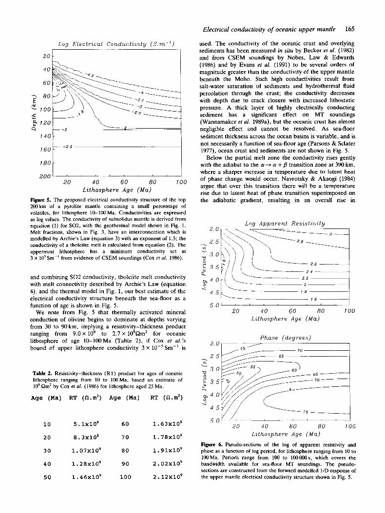
Figure 5. The proposed electrical conductivity structure of the top 200km of a pyrolite mantle containing a small percentage of volatiles, for lithosphere 10-100 Ma. Conductivities are expressed as log values. The conductivity of subsolidus mantle is derived from equation (1) for S02, with the geothermal model shown in Fig. 1. Melt fractions, shown in Fig. 3, have an interconnection which is modelled by Archie's Law (equation 3) with an exponent of 1.5; the conductivity of a tholeiite melt is calculated from equation (2). The uppermost lithosphere has a minimum conductivity set at 3 x lo5 Sm-' from evidence of CSEM soundings (Cox et al. 1986).

and combining SO2 conductivity, tholeiite melt conductivity with melt connectivity described by Archie's Law (equation 4), and the thermal model in Fig. 1, our best estimate of the electrical conductivity structure beneath the sea-floor as a function of age is shown in Fig. 5.

We note from Fig. 5 that thermally activated mineral conduction of olivine begins to dominate at depths varying from 30 to 90 km, implying a resistivity-thickness product ranging from 9.0 X lox to 2.7 X 109QmZ for oceanic lithosphere of age 10-100Ma (Table 2), if Cox et al.'s bound of upper lithosphere conductivity 3 X lop5 Sm-' is

Table 2. Resistivity-thickness (RT) product for ages of oceanic lithosphere ranging from 10 to 100Ma, based an estimate of lo9 Qm2 by Cox et al. (1986) for lithosphere aged 25 Ma.

Age (Ma) RT (n.m2) Age (Ma) RT (n.m2)

2 . 0 Log A p p a r e n t R e s i s t i v i t y

1 8

1 6

5 0 40 60 80 100

445Ec 20 L I L I '

Li thosphere Age ( M a )

P h a s e ( d e g r e e s ) 2.01- - / 1

2.5

3.0

T w L

: g 3 .5 4.

10 5. lXlO8 60 1. 63x109

20 8. 3x1O8 70 1. 78x109

30 1. O7x1O9 80 1 . 9 1 ~ 1 0 ~

40 1. 28x109 90 2 . 0 2 ~ 1 0 ~

50 1. 46x109 100 2 . 1 2 ~ 1 0 ~

5 . 0 ' ' I

20 40 60 80 100 Lzthosphere Age (Ma)

Figure 6. Pseudo-sections of the log of apparent resistivity and phase as a function of log period, for lithosphere ranging from 10 to 100Ma. Periods range from 100 to 100OOOs, which covers the bandwidth available for sea-floor MT soundings. The pseudo- sections are constructed from the forward modelled 1-D response of the upper mantle electrical conductivity structure shown in Fig. 5 .


temperature of approximately 55 “C. Experimental laboratory conductivity measurements have been made on /%spinel (Akimoto & Fujisawa 1965), but the results are probably not reliable (Duba 1976). However, a rise in conductivity to approximately 1 Sm-’ averaged over the interval 400- 670 km is a pervasive feature of all global conductivity profiles (Banks 1969, 1972; Campbell 1987). This conductivity, while not shown in Fig. 5, is included in the later thin-sheet models, as the sharp rise in conductivity has a significant effect on sea-floor MT soundings.

Fig. 6 shows the 1-D forward MT response of the upper mantle electrical structure shown in Fig. 5, as apparent resistivity and phase pseudo-sections. These are not true 2-D pseudo-sections, as they are compiled and contoured from 1-D forward calculations, but when the age scale in Fig. 5 is converted to length using typical half spreading- rates, a vertical exaggeration of -10 is evident, making the 1-D approximation justified. Little variation in the MT response is seen in Fig. 6 as a function of age; even less variation occurs if the upper mantle is dry with no melt fraction beneath lithosphere away from the ridge-axis. Thus, from Fig. 6, we can see that differences in electrical conductivity structure which may be resolved using real sea-floor MT soundings (containing errors of the order of 5 per cent) are restricted to lithosphere younger than 40 Ma.

2 SEA-FLOOR MT SOUNDING DATA

2.1 Introduction

We will examine three sea-floor MT soundings presented by Oldenburg (1981), collected on 1 Ma (‘JDF‘), 30Ma (‘CAL‘) and 72 Ma (‘NCP) lithosphere for compatibility with our petrological conductivity model. These are by no means the only sea-floor MT soundings available and their vintage prevents them from necessarily being of the best quality, but our objective is to illustrate principles of interpretation and obtain representative estimates of sea-floor conductivity as measured by the MT method. The tabulation of the data by Oldenburg, his own extensive examination of the inversion problem in Oldenburg (1981) and Oldenburg et al. (1984), a later re-interpretation of the data by Tarits (1986) and the span of lithospheric age makes them convenient for our purposes.

Oldenburg (1981) presented the argument that an observed peak in conductivity was associated with the seismic low-velocity zone and partial melting, and had a depth which depended on lithospheric age (from about 60 km for JDF to 200 km for NCP). In spite of a further examination by Oldenburg et al. (1984), (and also Tarits 1986) in which it was shown that such a simple and unambiguous interpretation was not possible, the concept of a peak in conductivity decreasing in magnitude and increasing in depth with increasing age fits so well with current models of lithospheric formation that it is generally and uncritically accepted as being true. Precise plots of ‘depth to conductor’ versus square root of age are often presented (e.g. Law 1983). We will show that the age dependence probably exists, but that it is not necessarily in the form that Oldenburg (1981) presented, and that the one-dimensionality of two of the three sites is questionable.

2.2 Tests for dimensionality

Until very recently, the usual approach to interpreting MT sounding data sought models which minimized the least-squares misfit between the model response and data. One-dimensional models were usually parametrized as layers or, in rare cases, continuous functions of conductivity with depth, and an iterative linearized approach was taken to finding the best-fitting model. However, Parker (1980) and Parker & Whaler (1981) showed that a model which minimized misfit was composed of delta functions of conductivity in an otherwise insulating half-space (they called this a D+ model). Since the least-squares minimizing model (D+) is not even in the same model space as those usually sought (layers, etc.), the models obtained from the usual least-squares methods owe as much to the construction of the model space as to the data being fitted. We are, perhaps, fortunate that D+ models are not physically reasonable, and so no one has been tempted to present one as a true model of Earth. The utility of D+ inversion lies in bounding the ability to fit a given set of data, and for testing the idea for compatibility with the assumption of one-dimensionality. We shall apply D + to the MT data in question, as did Oldenburg et al. (1984).

Parker & Whaler’s (1981) D + approach is, strictly speaking, only valid if the data are represented as Schmucker’s c values. MT data are most commonly represented as apparent resistivity and impedance phase, and Oldenburg (1981) presented the magnitude and phase of the admittance. In order to present our analysis we converted admittance to c. The estimation of errors is not trivial, and Oldenburg et al. (1984) used a Monte Carlo simulation to convert errors in admittance to errors in c. We used only the error on magnitude to generate equal errors on real and imaginary components of c, since the admittance phase and amplitude errors were generally consistent with the assumption of equal errors for the real and imaginary components, which would have been the error partitioning for the time series analysis of the original data. The soundings CAL and NCP were collected by J. H. Filloux of Scripps Institution of Oceanography, who has revised the calibration of the magnetometers used to collect these data, and accordingly we have multiplied Oldenburg’s admittance amplitudes by 1.215 for these stations. The transformed data and new errors are presented in Table 3.

We measure misfit of model response to data as the square root of the mean of the squares (RMS) of the weighted residuals. That is, for N data (dl, d Z , . . . , 6,) with errors (el , e, , . . . , e N ) and model response (dl, d2, . . . , &), the RMS misfit is defined as

The expected value of the sum of squares, on the assumption of independent and Gaussian errors, is N, and so the expected value of the RMS measure is 1, independent of the number of data.

The D + misfits for JDF, CAL and NCP are RMS 0.752, 1.269 and 0.965, compared to 0.674, 0.816 and 0.935 presented by Oldenburg et al. (1984). The differences indicate the different approaches to error estimation. On the


Table 3. The c values used for the data analysis presented in this paper, generated from the admittance data of Oldenburg (1981). Period is in seconds, real and imaginary parts of c and the errors are in metres. It is assumed that the error is equal for the two components of c.

NCP ( 7 2 Ma) CAL ( 3 0 Ma) JDF (1 Ma)

period

( 8 )

897

1266

1807

2560

3614

5120

7228

10240

14460

17980

24990

52560 -22320 9137

56830 -21830 6437

69060 -35210 6477

75420 -45340 7983

100900 -51420 9584

87620 -78920 14850

145300 -113500 23640

180100 -173900 53070

149600 -97170 45630

154900 -75610 59200

207200 -105600 93860

1500

2093

3243

4737

7200

9474

12414

15652

20000

25352

35294

60000

56460 -28780 15940

78260 -34860 16600

101300 -47260 7354

117600 -59960 7865

135600 -63290 9029

143500 -73190 9628

177500 -82830 12740

202900 -86180 13270

245300 -99180 15770

267700 -108200 17320

332300 -101700 22470

413900 -95670 38120

face of it, the soundings are all compatible with a 1-D model of conductivity; although our estimation of misfit for CAL exceeds the expected value, 1.269 is close to the 95 per cent confidence level, and so one would probably accept these data as 1-D. However, D + minimizes the Euclidean 2-norm (L2) of the misfit, and the use of the RMS statistic to test this number assumes both Gaussian and independent data errors. Thus, a full test of one-dimensionality using D+ should include a test of the residuals for normality and independence. By inspection of Fig. 7, only JDF has residuals that do not exhibit serial correlation (i.e. lack of independence). A rigorous test for independence of residuals is given by Crow, Davis & Maxfield (1960). Defining a run as an unbroken series of residuals which are either all positive or all negative, then the number of runs in a residual data set is a function of the correlation of the residuals (Crow et al. 1960, pp. 83-85). Applying the runs test to three MT soundings shows JDF residuals to be random, CAL to be non-random, and NCP to be borderline (residuals with this pattern of signs would only be generated 5-10 per cent of the time). It is interesting to note that the general form of the residuals is similar for both CAL and NCP (a dip in the imaginary component at about 1OOOOs followed by a steady increase, and a steady decline in the real component with increasing period). This suggests that a similar source-field contamination or other distortion might be common to both soundings.

It is interesting to consider the implications of serial correlation in residuals from D + for other inversions of the data. Df minimizes the L, norm of the residuals, not their serial correlation, and so optimization for independence of residuals will produce models different from those produced by Df inversions, although probably similarly rough. However, relaxation of misfit to produce maximally smooth models inevitably increases serial correlation in residuals as the inversion scheme expends the misfit budget selectively to achieve a smooth model (Constable, 1991). We note

1869 109500 -53420 7272

2321 109100 -58040 7536

3233 116000 -56620 8266

4780 131700 -82360 9253

6033 133500 -65150 8098

11270 177100 -98210 14170

16240 240800 -128100 25870

23180 265200 -135200 22180

33210 336900 -179200 32470

58540 380300 -237700 38030

105900 556700 -296100 94580

3

2 JDF w e i g h t e d r e s i d u a l s

-3'11 I I 1 I I 1 1 1 1 I I I I 1 1 1 1 1

1 O3 1 O4 1 O5 3

2 A CAL weagh ted re sadua l s

0

O O O O A A I I I I I 1 1 1 1 I I a I l 4 l l l l

1 o3 1 0 4 105 3

2 NCP w e i g h t e d r e s i d u a l s

I I I I I I I I I I I 1 1 1 1 1 1 1 1

103 1 O4 1 0 5 Per iod (s)

Figure 7. Weighted residuals after fitting D+ models to the three sea-floor MT data sets expressed as Schmucker's c values, as given in Table 3. The triangles are the real component residuals and the octagons are the imaginary. Trends spanning a decade of period are evident in both real and imaginary residuals for CAL and NCP, while JDF residuals appear uncorrelated.


therefore that if residuals from D + are not independent, they are not likely to be independent when other presently available inversion methods are used.

Using a Kolmogorov-Smirnoff test, the distribution of the JDF weighted residuals is indistinguishable from Gaussian. The mean is 0.01, and since the standard deviation of the mean is 0.16 they must also be considered zero mean. Our last question is the matter of magnitude. They are, on average, 0.75 in size, as the D + misfit has already indicated. The expected value is 1.0, but we would expect D+ to fit better than the expected value. To find out just how much better D+ will fit this data set we have conducted a simulation, described below.

2.3 Introducing a simulation

We have generated 18 data sets, with noise, from a fixed model and performed a D + inversion on all of them. The model comprises two layers; 100 8 m decreasing to 1 8 m at a depth of 300 km. We shall see that this is similar to the underlying character of models which fit the real data. The data were computed at 12 periods between 1500 and 100OOOs, again similar to the real data in question. Eighteen different realizations of 10 per cent noise were applied to the data, and were inverted using the D + algorithm. The resulting misfits varied between 0.67 and 1.01, with a mean of 0.8 and a standard deviation of 0.1. Thus an overfit to RMS 0.75 for JDF does not seem inconsistent with the assumption that the errors have been well estimated. It is interesting to note that one of the realizations has a misfit which exceeds the expected value of RMS 1.0. From a statistical perspective this is not at all surprising, but from the data gatherer's and interpreter's point of view it is a sobering reminder that even objective statistical guidelines for data analysis will only be appropriate on average, and may fail for the occasional data set.

It appears that the JDF data are totally consistent with the usual assumptions of one-dimensionality and well-estimated, zero mean, independent, Gaussian errors. The smoothest (in the sense of the integrated &-norm of first derivative) model which has the expected misfit of RMS 1.0 (Constable, Parker & Constable'1987) is shown as the broken line in Fig. 8, and is our preferred model for these data. A peak in conductivity (trough in resistivity) is barely perceptible at 70km depth. Some authors (e.g. Oldenburg et al. 1984; Smith & Booker 1988) prefer to consider fits at the 95 per cent confidence level, which in this case is RMS 1.24, by which stage nearly all structure has disappeared, leaving only a factor of three increase in conductivity at about 30 km depth. Thus we see that the peak in conductivity, accepted for many years as an intrinsic feature of the oceanic lithosphere, is not required by an objective interpretation of the JDF sounding. It should be made quite clear that we have not disproved the existence of a high-conductivity zone, as we cannot know what the true misfit for the JDF sounding is nor how much structure is actually present in Earth, but only that it is not a required feature of the upper mantle for the purposes of interpreting these data.

We have shown that the soundings CAL and NCP are not consistent with our assumptions regarding noise and dimensionality, and so a similarly objective interpretation

t---

JDF s m o o t h m o d e l s

-.. \ \ I / I . "

103 104 105 106 ----.,CAL s m o o t h m o d e l s

-

- I 1 I 1 1 1 1 1 1 I I I I I I I I I I

2 100 -

; 10-1 - '+ v, NCP s m o o t h m o d e l s v)

I I 1 1 1 1 1 1 1 I I I I I I I I I I I I

103 104 1 0 5 106 Depth ( m )

Fiiure 8. Maximally smooth models generated by the Occam inversion algorithm of Constable er af. (1987) which fit the various data sets to various misfits. For each data set the misfits are between about 1.02 and 1.5 times the D+ misfit. The vertical lines indicate the positions of delta functions in the D+ models. The broken line for JDF is the expected (RMS 1.0) misfit model.

cannot be made for these data. In particular, we cannot assume that a fit to RMS equal to 1.0 is at all significant for them. On the other hand, many practitioners of the MT method would support the idea that an approximation to an average 1-D structure is recoverable from data that do not have independent Gaussian errors and/or are mildly distorted by higher dimensional structure. With this philosophy in mind, and in order to illustrate some aspects of MT interpretation, data from CAL and NCP are subjected to 1-D inversion. We hope, however, that the reader will bear in mind that only JDF is fully compatible with the assumption of one-dimensionality.

Our simulation suggested that D + overfit 1-D by about 1.25. Using D + as an index of data quality, we will consider the smooth inversions which fit to RMS 1.0, 1.6 and 1.2 for JDF, CAL and NCP as preferred models for these data sets. These models are plotted in Fig. 9 along with the laboratory predictions developed in the previous section. While one would not expect an MT experiment to be sensitive to the low conductivities predicted for depths above 50 km, it is apparent that the MT derived conductivities are systemati- cally higher than one would expect from studies of olivine conductivity, at all depths. In the next section we consider the coast effect as a possible reason for this bias.


smooth model and one approximating the D’ models is not necessarily well behaved or predictable. Thus we see in the CAL models that at 200 km a conductivity trough becomes a peak in conductivity as the RMS misfit is decreased. In NCP models the depth of the shallow peak in conductivity migrates with misfit. Smith & Booker (1988) argue that D+ delta functions smoothed through Backus-Gilbert resolving kernels yield a good approximation to the smooth models. However, we have shown in Fig. 8 that the peaks do not necessarily form at all the positions of the D + conductance spikes.

Although the magnitude of the conductivity peak is clearly dependent on misfit, even the existence of a region in the mantle that has a higher conductivity than shallower and deeper material would be significant, so we would like to know whether a peak exists at all. It might be that the conductivity peaks are in fact fitting noise in the data, rather than structure. To examine this possibility we use the simulated data introduced above, which have been manufactured under ideal conditions of model dimensionality and noise statistics. We have fit smooth models to all but one of the simulated data sets to yield a misfit of 1.0. These models yield an accurate, but smoothed, reproduction of the true starting model. If the exercise is repeated with a misfit of 1.05 times that produced by D+, about half these models feature structure which differs greatly from the starting model. The eight most ‘interesting’ overfitting models are shown in Fig. 10, along with the corresponding models which fit to RMS 1.0. The overfit models include an assortment of conductivity peaks between 30 km and 150 km depth. We know that all these peaks are a result of fitting noise in the data, yet a comparison between Figs 8 and 10 shows that the simulation reproduces the features observed in the better fitting data models very well. It is notable that the ‘interesting’ models are not restricted to the cases where the data can be fit much better than the expected value. Misfits for the overfitted smooth models are 0.725, 0.785, 0.815, 0.816, 0.844,0.889, 0.953, and 0.955, covering almost the whole range of minimum misfits produced by the simulation. The conclusion is that one can indeed obtain models which feature a high-conductivity layer, similar to that which has been presented for the oceanic upper mantle, when such a layer does not exist in the real model, or Earth.

The ability to produce peaks in conductivity at various depths simply by overfitting synthetic data should make one sceptical of the high-conductivity peaks found for the real data sets, and also reduces the significance of the depths associated with those peaks. In spite of the aspersions that we are casting at previous interpretations of these data sets, we are left with the observation that ifethe data are overfit then the depths of the conductivity peaks do increase with lithospheric age, although one must note that the inability to pass tests for one-dimensionality and poorly behaved error statistics forces us to consider a quantitative interpretation of the CAL and NCP data which may not in fact be justifiable. We do think that the original hypothesis presented with these data (that conductivity structure migrates deeper with increasing age of the lithosphere) is still tenable. Although these peaks are not required by the data, we have not demonstrated that they cannot exist, and perhaps they do reflect the real structure of the oceanic upper mantle after all. There is clearly scope for extending

1 0 4 - \

...... -

I I

7 E c: 104

10 Ma Pred ic twn .- - - . - -

. ....... ....

-

a,

\ _’ -.: JDF Model I

30 Ma Predrc twn 1 1

1 0 4 1 0 5 106

c 1 0 4 1

w z 10‘

1 0 0

70 Ma Predict ion I c I - - - - - - - - - -

I I I 1 I I I I I I I 1 1 1 1 1 1

1 0 4 1 0 5 106 D e p t h (m)

Figure 9. Smooth inversions of sea-floor MT data fitting to an RMS misfit 1.25 times the minimum RMS misfit obtained from D+; these are our preferred models for JDF, CAL and NCP under the assumption that the Earth structure is locally 1-D (lower curves in each figure). The upper curves are predictions of the electrical conductivity structure for 10, 30 and 72 Ma lithosphere from Fig. 5.

2.4 The significance of the conductivity peak

Oldenburg’s interpretation of all three soundings featured a peak in conductivity at around 100km, with depth increasing with age. This high-conductivity zone was interpreted as a region of partial melting, and melt fractions were computed from the peak conductivities. However, the development of smooth inversion algorithms (Constable et al. 1987; Smith & Booker 1988) has shown that the size of peaks in conductivity for 1-D models increases with decreasing data misfit. In the extreme, the D’ models, which fit the data best of all in an L, sense, have infinite peaks in conductivity in an otherwise infinitely resistive Earth. Thus, peak conductivity and associated peak melt fraction will be a function of data misfit. This is illustrated in Fig. 8 for the three MT examples, where we have used the algorithm of Constable et af. (1987) to generate maximally smooth models which fit the data between about 1.02 and 1.5 times the D+ misfit. Not only the magnitude of the peak, but also its existence, depends on what level of misfit is chosen to be appropriate.

Fig. 8 also illustrates some other points of MT interpretation. The transition between a poorly fitting

G. Heinson and S . Constable

Smooth m o d e l s (RMS = 1 00)

03

Dashed line . Start Model lo- ' I I 1 l l 1 1 1 l I I I 1 1 1 1 1 1 I I 1 1 1 1 1

1 o3 lo4 105 1 0 6

S m o o t h Models (RMS = 1.05 x misfit of D f ) 1 0 4

I

I o3 1 0 4 1 O5 106 D e p t h (m)

Fiiure 10. The eight most 'interesting' overfitted models from a simulation in which 18 noisy data sets were generated from the forward MT response of a two-layer model (shown by the dashed line). Overfitting was accomplished by generating maximally smooth models which fit to within 5 per cent of the D+ misfit. For comparison, the models which fit to the expected RMS 1.0 are shown.

the modelling to other data sets and testing for compatibility with this hypothesis.

3 THIN-SHEET MODELLING

3.1 Introduction

Non-uniform induction due to the shape of the ocean basin (e.g. Wannamaker et al. 1989b; Ferguson, Lilley & Filloux 1990) and from changes in sea-floor topography (Filloux 1981; Heinson et al. 1991) may profoundly influence MT observations on the sea-floor. The electrical conductivity of salt-water decreases rapidly with temperature from at most 5Sm-l at the sea surface to attain a relatively uniform 3.2 Sm-' through most of the water column to the sea-floor, making it several orders of magnitude more conductive than the oceanic lithosphere. The extent of 3-D induction in the ocean is difficult to quantify as there are few practical numerical modelling algorithms which are suited to 3-D problems, although analogue modelling techniques can provide useful information on coastal induction effects (e.g.

Chen, Dosso & Nienaber 1989). Previous analysis of sea-floor MT observations has required a number of assumptions about the nature of the 3-D induction. For example, single site MT interpretations have been undertaken using invariant impedance estimates (e.g. Filloux 1981) and transverse electric (TE) component impedance estimates (e.g. Ferguson et al. 1990), whilst 2-D array studies have also made use of the transverse magnetic (TM) component impedance estimates (e.g. Wannamaker et al. 1989b).

In this section we investigate 3-D induction in an ocean basin using a thin-sheet algorithm of McKirdy, Weaver & Dawson (1985), and in particular we examine how the sea-floor MT observations from Oldenburg (1981) can be reconciled with the profiles based on laboratory conductivity data and CSEM results of Cox et af. (1986), shown in Fig. 5. The thin-sheet method is one of the few practical techniques available to forward model 3-D EM problems: theory and practical algorithms have been discussed by several authors and the reader is referred to Price (1949), Vasseur & Weidelt (1977), Ranganyaki & .Madden (1980). Weaver (1982) and McKirdy et al. (1985) for further details.

A thin-sheet model is ideally suited to analysing the effect of a laterally variable surface conductor, overlying a stack of layers which represent a 1-D Earth. Observations of natural source variations in Earth's magnetic field on the sea-floor are made in the range of periods from 100 to 10000Os, which provide information in the depth range 50-500 km. At such periods, the EM skin depths in the ocean, and in oceanic lithosphere, are large in comparison to the depth of the ocean, so that the ocean may be approximated by a sheet of negligible thickness. A factor which makes thin-sheet modelling of ocean basins very appealing is that the geometry of the coastlines and bathymetry are known and that the conductivity of sea-water is approximately uniform. Thus, the surface thin-sheet can incorporate accurate a priori information, with resolution of surface conductance changes being dependent primarily upon resolution of the grid used in numerical calculation. Underlying the thin-sheet, a suitable 1-D structure can be determined using our conductivity model for the oceanic upper mantle, shown in Fig. 5. Such thin-sheet models represent an extreme case of uniformly resistive lithosphere extending under both ocean and continent crust, with no major leakage paths to the deep conductive structure.

3.2 Model description

Simple ocean basin configurations, shown in Fig. 11, are incorporated into a thin-sheet, comprising a uniform depth ocean, with oceanic and continental crust. The thin-sheet is 5 km thick, which overlies a 1-D model derived for lithosphere of age 70Ma, shown in Fig. 5. This age of lithosphere was chosen as being appropriate for the mean square root age of the Pacific. Although this choice is somewhat arbitrary, it can clearly be seen from Fig. 5 that electrical structures are similar for lithosphere older than 40 Ma. The thin-sheet model parameters are listed in Table 4. The thin-sheet models shown in Fig. 11 are not intended to be direct representations of real ocean basins, owing to the limitation of a 1-D substructure and the coarseness of the numerical grid used, however, the shape of the basins


I

4 0

C % B

Model I: Closed Ocean Basin

- - 7885km

Model 11: Open Ocean Basin

Model V: Ocean Layer

Model 111: Ocean Channel

Model 1V: Single Coastline

Figure 11. Five simple ocean basin geometries modelled by the thin-sheet method. The continental margins are shown by the hatched regions. Models I and I1 have 3-D geometries, models I11 and IV are 2-D, and model V is included for the 1-D response of the substructure. The thin-sheet is 5 km thick, and comprises of continental crust and salt-water with conductivities 0.005 and 3.3 Sm-' respectively. Each thin-sheet is parametrized as discrete conductance values at each grid node of a 20 X 20 regular grid, with grid node spacing is 415 krn. MT parameters are calculated along transect A-A' at grid nodes 1-3, which are approximately 623, 1453 and 2283 km from the coastline at A'.

has simple analogues: for example, the north Pacific and Indian Ocean for the open ocean basin (model 11); Atlantic and Tasman Sea for the open ocean channel (model 111); and the Pacific coast of South America for the single coastline (model IV). The thin-sheet configurations can be classed into two groups: the closed and open ocean basins (models I and 11) have 3-D geometries, while the ocean channel and single coastline (models 111 and IV) are 2-D. A 1-D forward calculation from the underlying structure with an Ocean layer of infinite extent, can also be made (model V). Thus, 1-D, 2-D and 3-D induction effects in an ocean basin may be compared.

Thin-sheet calculations were made at six periods, from lo00 to 100o00s, spaced evenly in log domain. The electric and magnetic fields at the bottom of the thin-sheet can be used to calculate MT parameters of apparent resistivity and phase, along a 'sea-floor' transect A-A' at grid nodes 1-3,

Table 4. Parameters used in thin-sheet models of the ocean basins. The profile is representative of 70 Ma lithosphere, with a partial melt zone from 84 to 136 km. The melt conductivity is calculated using Archie's Law with an exponent of 1.5. The thin-sheet grid comprises 20 x 20 nodes, with a grid node spacing of 415 km.

Description Conductivity ThicknssS

(S . d) (m)

Thin-sheet Paramet-

Continental crust 0.005 5000

Sea-water 3 . 3 5000

70 Ma W D h e r e P m

Sheeted dykes 0.0003 5000

Upper lithosphere 0.00003 58000

Lithosphere 0.003 16000

Asthenosphere 0.005 52000

Adiabatic upper mantle 0.003 254000

Transition zone 0 . 2 280000

Lower Mantle 1.0 00

Depth to

Baa0 (m)

5000

5000

10000

68000

84000

136000

390000

670000

m

shown in Fig. 11. We consider the 3-D effects in MT parameters parallel (TE) and perpendicular (TM) to the north-south striking coastline, assuming that this is the dominant 2-D strike in conductivity structure.

3.3 TE and TM, MT response

Figs 12(a) and (b) show synthetic MT parameters of apparent resistivity and phase as a function of period, polarized parallel to the coastline (TE), for the thin-sheet models I-IV. Also shown in each figure is the 1-D response of the underlying structure from model V. There are significant differences between 1-D, 2-D and 3-D models at all periods. The 3-D apparent resistivities of models I and I1 are attenuated by factors ranging from 10 to 100 relative to the I-D apparent resistivity, and the phase also shows large differences. This attenuation is greatest, and almost independent of period, for model I. By contrast, the attenuation reduces with period for model 11. There is no significant difference between sites at different grid nodes, except at the grid node 1 closest to the coastline, where the short period apparent resistivities are significantly higher than at the other sites. Models 111 and IV have a 2-D geometry and show close agreement at all periods, except at 1o00s. At longer periods, they recover the 1-D apparent resistivity response of the underlying structure.

It is interesting to note that close to the coastline at site 1, the TE phase is greater than 90" for models I, I1 and 111, but not for the single coastline model IV, and the phase is greatest for the ocean channel model. This has been observed (e.g. Ferguson 1988) in the Tasman Sea, which approximates the ocean channel model (model 111). Away from a single coastline, the phase is similar to the 1-D forward response. This example illustrates clearly that the presence of a second 2-D coastline, even many thousand of kilometres away, may profoundly alter a single coastline


1 03

102

10'

1 0 0

103 1 o4 1 05 Period (s)

103 1 0 4 1 05 Period ( s )

7 160

-e 0 120 L

Q 80

40 2

c I

0- 103 I o4 I o5

Period ( s )

1 0 3 2

G ft

c: 102

vi 10'

100

10-1

L

a

0

0

+

1 03 1 0 4 1 o5 Period ( s )

Closed Ocean B a s i n

Open Ocean B a s i n

Ocean Channel

S ing le Coastl ine

I D Model

80

60

I o3 1 0 4 I 0 5

Period ( s )

0- 1 o3 I o4 1 05

Period (s)

0 Closed Ocean B a s i n

A Open Ocean B a s i n

0 Ocean Channel

0 S i n g l e Coast l ine

+ I D Model

Figure U. (a) TE apparent resistivity curves at grid nodes 1-3 along transect A'-A, for the five thin-sheet models. The grid node position is shown in the top right-hand corner of each figure. (b) As for (a), but for TE phase curves.


(a) 1 03

c 102 -3

vi Q 10'

L

K

R R

1 0 0

lo-'

103 2

G

c 102

ui 10'

loo

L

1 o3 104 1 o5 Period ( s )

103 104 1 05 Period ( s )

2 $ Q, 20 401 0 u 103 104 1 05

Period (s)

1 03

c: 102

bi 10'

1 0 0 d 10-1

2

G

L

R,

1 03 1 04 1 o5 Period ( s )

0 Closed Ocean Basin.


0 Ocean Channel

0 Single Coastline

-+ 1D Model

0- 1 03 1 o4 1 o5

Period ( s )

0 Closed Ocean B a s i n


0 Ocean Channe l

0 S i n g l e Coast l ine

+ 1D Model

Figure u. (a) As for Fig. 12(a), but for TM apparent resistivity curves. (b) As for Fig. 12(b), but for TM phase curves.


interpretation as the electrical compensation distance in the Ocean from the coast, above a resistive oceanic lithosphere, is comparably large (Cox 1980).

The TM apparent resistivities are considerably smaller, by a factor of 100-1O00, than the 1-D forward response, due to electric charge accumulation at the coastline for both 2-D and 3-D ocean basins. These are shown in Figs 13(a) and (b). In particular, there is close agreement for models I, I1 and 111 where the ocean is bounded north-south on two sides. Single-coastline model IV shows greater apparent resistivity which approaches the 1-D forward response at the longest periods. Thus, TM estimates are relatively insensitive to 3-D induction effects, but they are sensitive to the inclusion of additional 2-D structure, such as a second parallel coastline.

At the centre of the closed ocean basin (model I), the MT response is naturally isotropic, due to the symmetry. However, the MT parameters do not recover the 1-D response; the apparent resistivities are attenuated by a factor of approximately 100. In the general case, TE and TM apparent resistivities for both 3-D thin-sheet models I and I1 are attenuated from the 1-D response, by factors which vary from 10-1OOO. As all Ocean basins are 3-D to some extent, it suggests that real sea-floor MT apparent resistivity observations will be similarly reduced from the 1-D response of the upper mantle. An important conclusion is that single-site MT interpretations will inevitably produce conductivity profiles that are too conductive. Better interpretations may result from a 2-D model using TM apparent resistivities and phase which are more robust to 3-D structure (Wannamaker et al. 1989a,b).

The 2-D and 3-D induction effects are thus shown to be significant, and an important corollary to this result is that such induction effects introduce a complicated and unpredictable distortion of the MT parameters. The 1-D MT response of the underlying structure, shown in Figs 12(a) and (b), varies smoothly with period, and indeed neither apparent resistivity nor phase indicates any major complexity in the electrical substructure. By contrast, the synthetic 3-D MT response at the sea-floor sites contains many spurious peaks and troughs, which if interpreted as a 1-D structure would result in misleading conductivity profiles. In addition, thin-sheet ‘sea-floor’ MT data (with random Gaussian noise added) are not, in general, compatible with a 1-D profile when tested with D’.

Thin-sheet models described previously represent an extreme case, which may serve as an upper bound to 2-D and 3-D induction effects in the ocean. Leakage paths in real ocean basins to the deep conductive parts of Earth, such as a subducting slab or spreading ridge may reduce this attenuation significantly. However, the effect of these leakage paths and their distribution in the ocean basins is a matter of speculation and, as we shall see, our extreme model reproduces some features of the field data.

3.4 Comparison between theoretical and observed MT parameters

It has been noted that there is little or no anisotropy in the MT response at the centre of the closed ocean basin model (model I). Away from the coastlines the anisotropy is less than a factor of 10 in both 3-D models (model I and 11),

whereas the 2-D models (model 111 and IV) have much higher anisotropy. This result is consistent with observed low anisotropy in the MT response in the north Pacific (e.g. Filloux 1977, 1980; Wannamaker et al. 1989a), which has a geometry similar to model 11, and the much higher anisotropy in the Tasman Sea (Ferguson et al. 1990), which is similar to model 111. Such low anisotropy in the north Pacific is often cited to argue the case for a smaller coast effect than is consistent with the resistive upper lithosphere determined by CSEM. We show that the coast effect in our thin-sheet models with two or more coastlines strongly distorts the MT response across the whole ocean basin, and that low anisotropy is characteristic only of the geometry of the coastlines.

Fig. 14 shows the MT estimates with one standard error from sea-floor sites JDF, CAL and NCP (Oldenburg 1981), the 1-D sea-floor MT response of model V, and the TE sea-floor MT response from model I1 at grid nodes in the thin-sheet which approximate the location of the actual observation site with respect to the surrounding coastlines. It is clear that the observed apparent resistivities are smaller than the 1-D theoretical values. This difference is dependent upon period, with attenuation ranging from a factor of -10 at the shortest period, to a factor of 2-3 at the longest period. The observed apparent resistivities and phases are relatively flat over two decades of period, with the indication of a dip at a period of approximately 1OOOOs. This morphology is well modelled by the 3-D calculations for model I1 (open ocean basin), although the thin-sheet apparent resistivities are depressed more than the data for CAL and NCP. The similarity in phase for all three sites is particularly striking.

Although the apparent resistivity from the thin-sheet model is less than that observed at CAL and NCP, we have noted that the attenuation exhibited in the thin-sheet models is probably more extreme than exists for real Ocean basins as we have included no leakage paths to the deeper parts of the mantle. It has been suggested by Wannamaker et al. (1989b) that a subducting slab may act as a leakage path for induced electric currents in the ocean to the deeper and more conductive parts of Earth’s upper mantle. Other low resistance paths, such as spreading ridges, fracture zones and hot-spots, might also exist. Even passive margins may provide leakage paths through continental lithosphere (Kellett, Lilley & White 1991) These factors complicate a simple 3-D interpretation in terms of conductive Ocean/resistive lithosphere contact. Leakage through the oceanic lithosphere is dependent upon its resistivity- thickness product, the magnitude of which is of some debate. CSEM data have indicated that the lithosphere is extremely resistive (Cox et al. 1986), although Vanyan et al. (1990) have argued that anisotropy in the lithosphere manifests as fluid-filled cracks, may improve vertical conductivity and thus allow leakage of electric current through the lithosphere.

We argue, however, that the zeroth-order differences between theoretical and observed MT parameters (Fig. 14) may be reconciled by 3-D EM induction effects in the Ocean alone. The conductance of the world Ocean (Fainberg 1980) is considerably greater than proposed leakage paths to the deeper part of the mantle (Wannamaker et al. 1989b), so that even in the presence of such leakage paths, 3-D


(C) Lithosphere Age . 72 Ma 103 I

(a) Lzthosphere Age . 1 M a 103 &-

? s c 102 L

vj

e R G T

10‘

1 0 0

90 j

2 20

I ’

10 0 I I 1 I I I I I I I I I 1 I 1 1 l 1

105 1 0 3 1 0 4 Period (s)

(b) LithospheTe Age . 30 Ma 103 1

c 102 L

ui a: 01

10‘ R R T

100 I 03 104 105

90

8 o k T T

40

$ 301 20

lo> 0 1 03 104 1 0 5

Period ( s )

Figure 14. (a) Apparent resistivity and phase estimates for JDF (error bars and small squares); the predicted sea-floor 1-D response from model V substructure; and the thin-sheet MT response (triangles) in the three-sided basin model 11, at a grid node approximately corresponding to the location of the JDF experiment. (b) As for (a), but for CAL. (c) As for (a) but for NCP.

- s / i - c 102 L

ui

107

I I I I 1 1 1 1 I , 1 I 1 1 1 1 1

103 I o4 1 05 I

1 ° 7 0 1 03 1 0 4 1 0 5

Period (s) Figure 14-(conlinued)

induction effects due to the shape of the ocean basin are still paramount. We propose that accurate thin-sheet modelling of the ocean basins, using substructures determined in Fig. 5, and analysis of the full 3-D sea-floor impedance tensor may provide a means of calculating a good approximation to the 3-D induction effects from the ocean.

4 DISCUSSION A N D CONCLUSIONS

Our model of oceanic upper mantle conductivity based on laboratory data is one to two orders of magnitude more resistive than previous sea-floor MT interpretations have suggested. Part of the explanation results from the inclusion of a resistive uppermost lithosphere as indicated by CSEM experiments; MT data have an inherent lack of resolution of such resistive structures. However, this does not explain the systematic differences in the depth range 50-500 km, over which MT soundings have better resolution of the more conductive parts of the upper mantle. A number of mechanisms have been advanced to account for such differences. These have included making assumptions about the enhanced conductivity of grain boundaries (Shankland & Waff 1977); including a large percentage of partial melt (Oldenburg 1981; Wannamaker et al. 1989b); invoking carbon on grain boundaries (Duba & Shankland 1982); the presence of volatiles (Tozer 1981; Tarits 1986); and the presence of free hydrogen ions in a subsolidus mantle (Karat0 1990). Alternatively, faith in the laboratory data leads one to predict higher temperatures than are probably reasonable for the upper mantle (Constable & Duba 1990). We have turned the problem around and sought a modification of the MT interpretations, asking why the


models derived from sea-floor MT observations may be more conductive than can be supported by the simpler physical models. Complicating the MT interpretation by the inclusion of coastline structure avoids the necessity of the above-cited hypotheses for enhanced mantle conductivity. By demonstrating the effect of coastlines we have not excluded the possibility of other conductivity enhancing material in the mantle, but for the Pacific data we have considered here, the coast effect seems to be adequate to explain the data without modification of our olivine mantle. This may not be the case in other regions or for other data sets.

Although a great many assumptions have gone into the construction of our thin-sheet models of ocean basins, the important features of the results, namely the attenuation of apparent resistivity of sea-floor MT soundings from the 1-D response of the underlying conductivity structure, are primarily dependent on only two parameters; a lithosphere resistivity-thickness product of the order of lo9 Qm', and the inclusion of coastlines in the modelling. The CSEM sounding technique provides the most compelling evidence for such a resistive upper mantle, but other other observations, such as the distortion of land MT impedances (Mackie, Bennett & Madden 1988) and sea-floor MT impedances (Heinson 1991), are in agreement, and suggest that the result measured on a scale of 100 km by the CSEM experiments is applicable to much larger regions. A resistive layer is also expected from laboratory measurements of olivine conductivity applied to petrological and thermal constraints for the upper mantle. While the largest uncertainty in our model is the extent of leakage in geologically exceptional regions, the conductance of leakage paths to the mantle is at least orders of magnitude smaller than the conductance of the ocean.

Although the conductivity of the material underlying the resistive upper mantle will have only a secondary effect in comparison to the distortion due to the coastlines surrounding the ocean basin, it does, however, determine the magnitude of the MT response before distortion. To that extent our modelling is dependent on the values chosen for olivine conductivity, mantle melt conductivity, melt fraction, mixing laws and mantle temperature, volatile content and petroJogy, We have discussed uncertainties associated with these parameters in the text, and suggested bounds for mixing laws and temperature. Of all these free variables, the extent of melting, and consequently the connectivity of the melt fraction, presents the largest uncertainty in terms of conductivity. The large melt fractions previously suggested by interpretation of electrical conductivity studies have been addressed in this paper. Lower melt fractions used in our modelling are, if anything, higher than suggested by other geophysical measurements (e.g. Sat0 et al. 1989). Further- more, our models are not designed to be representative of structure in tectonically active regions. Close to mid-oceanic ridges the simple cooling slab approximation is inappropri- ate and dynamic models of mantle circulation should be used instead; such dynamic models (Phipps Morgan 1991) also predict lower melt fractions than those obtained from the cooling slab model. A reduction in melt fraction will make the influence of the coast effect persist over even greater distance-scales, although we note that the resistivity-thickness product from the CSEM experiment

used in our models has already made the compensation distance the size of the biggest ocean basins. Since melt fraction in our model is 2 per cent or less for oceanic lithosphere older than 30Ma, the effect of excluding melt completely will only produce a change of half an order of magnitude in the conductivity of the melt region and have even less effect on the sea-floor MT response. These secondary effects will have little impact on the zeroth-order models we have presented, but might be more important when specific data sets and realistic coastlines are modelled. It has been the purpose of this paper to demonstrate the importance of coastlines in the interpretation of sea-floor MT data, and it will be left for future work to consider the details of specific regions and data.

Our petrological model of mantle electrical conductivity in Fig. 5 shows that the conductivity of the oceanic upper mantle is indeed likely to be a function of age, as has been popularly assumed. However, the age dependence is strongest for lithosphere younger than 40 Ma. Predictions of upper mantle conductivity older than 40 Ma shows only subtle changes, with variations in the MT response of less than 0.1 decade in apparent resistivity and 5" in phase. Clearly, the noise level of sea-floor observations will have to be low before such an effect is seen. More importantly, the effect of coastlines will have to be included in the interpretation of sea-floor MT data. For Ocean basins surrounded by coastline on three sides, thin-sheet modelling shows that apparent resistivity is attenuated everywhere from the 1-D response of the underlying conductivity structure by 1-2 orders of magnitude. Even if the true effect of coastlines is only one tenth of that, it will still mask the effect of age. We also note from Fig. 5 that since the resistivity-thickness product is of particular importance in determining the distortion of sea-floor MT data, and is shown in Table 2 to be a function of lithosphere age, CSEM is an ideal tool for mapping the thermal evolution of lithosphere away from the ridge axis. Note that it is difficult to estimate the resistivity-thickness product from the MT data alone.

Re-analysis of published sea-floor MT responses has shown that the much cited high-conductivity layer is not in fact required by the data, and might simply be a result of overfitting the data. This raises the question of what a suitable level of misfit appropriate for a set of I-D MT data is if one does not have confidence in the expected level of misfit, or RMS 1.0. Numerical simulations using a simple two-layer model indicate that the D+ method will fit the data to to a misfit level of RMS 0.8 on average. That is, D' overfits the data by a factor of about 1.25 and, by using D+ as an index of data quality, we suggest that smooth inversions should be fit to an RMS tolerance which is 1.25 times greater than the D+ misfit. This rule of thumb can be refined for particular problems by conducting a simulation as we have done, choosing a simple model which reflects the important features of the data and a data spacing and quality appropriate for the case in question. In another extension of standard 1-D interpretation, we point out that a test on the magnitude of the RMS misfit resulting from D+ is not a complete test of compatibility with a 1-D model, and that the residuals should also be tested for independence using, say, a runs test and normality using a test such as the Kolmogorov-Smirnoff test.


ACKNOWLEDGMENTS

F. E. M. Lilley, C. G. Constable, R. L. Parker, I. N. Jackson, A. E. Ringwood, W. F. McDonough, L-G. Liu, G. F. Davies, B. L. N. Kennett, A. White and two anonymous reviewers are thanked for their comments and discussion which have improved this paper significantly. Most of the figures were produced with PLOTXY and CONTOUR kindly supplied by R. L. Parker. This work was conducted while GSH was a recipient of a Commonwealth Scholarship and Fellowship Plan Award a t the Australian National University and SCC was funded by the NSF under grant OCE 10245 and EAR 89 03222 and as a visiting fellow at the Australian National University.

REFERENCES

Akaogi, M., Ito, E. & Navrotsky, A., 1989. Olivine-modified spinel-spinel transitions in Mg,SiO,-Fe,SiO,: calorimetric measurements, thermochemical calculations, and geophysical application, 1. geophys. Res., 94, 15671-15685.

Akimoto, S. & Fujisawa, H., 1965. Demonstration of the electrical conductivity jump produced by the olivine-spinel transition, 1. geophys. Res., 70, 443.

Anderson, D. L., 1982. Chemical composition and evolution of the mantle, in High-pressure Research-Applicatiom in Geophysics, pp. 301-317, eds Manghnani, M. & Akimoto, S., Academic Press, New York.

Anderson, D. L. & Bass, J. D., 1986. Transition region of the earth’s upper mantle, Nature, 320, 321-328.

Banks, R. J., 1969. Geomagnetic variations and the electrical conductivity of the upper mantle, Geophys. J. R. astr. SOC., 17, 457-487.

Banks, R. J., 1972. The overall conductivity distribution of the Earth, J. Geomag. Geoelect., 24, 337-351.

Becker, K., Von Herzen, R. P., Francis, T. J . G., Anderson, R. N., Honnorez, J., Adamson, A. C., Alt, J . C., Emmermann, R., Kempton, P. D., Kinoshita. H., Laverne, C., Mottl, M. J. & Newmark, R. L., 1982. In situ electrical resistivity and bulk porosity of the oceanic crust Costa Rica Rift, Nature, 300,

Bina, C. R. & Wood, B. J., 1987. Olivine spinel transitions: experimental and thermodynamic constraints and implications for the nature of the 400 km seismic discontinuity, 1. geophys. Res., 92,4853-4866.

Brace, W. F., Oramnge, A. S. & Madden, T. R., 1965. The effect of pressure on the electrical resistivity of water-saturated crystalline rocks, J . geophys. Res., 70, 5669-5678.

Brown, J . M. & Shankland, T. J. , 1981. Thermodynamic parameters in the earth as determined from seismic profiles, Geophys. J. R. astr. SOC., 66, 579-596.

Bulau, J . R., Waff, H. S. & Tyburczy, J . A., 1979. Mechanical and thermodynamical constraints on fluid distribution in partial melts, 1. geophys. Res., 84, 6102-6108.

Campbell, W. H., 1987. Introduction to electrical properties of the Earth’s mantle, Pure appl. Geophys., US, 193-204.

Canas, J. A. & Mitchell, B. J., 1978. Lateral variations of surface wave anelastic attenuation across the Pacific, Bull. seism. SOC. Am., 68, 1637-1650.

Chen, J., Dosso, H. W. & Nienaber, W., 1989. Laboratory electromagnetic model results for EMSLAB region, J. geophys. Res., 94, 14167-14173.

Chopelas, A., 1991. Thermal properties of B-Mg,SiO, at mantle pressures derived from vibrational spectroscopy: implications for the mantle at 400km depth, 1. geophys. Res., 96,

594-598.

11817- 1 1829.

Constable, S. C., 1990. Marine electromagnetic induction studies, Geophys. Sum., 11,303-327.

Constable, S. C., 1991. Comment on ‘Magnetotelluric appraisal using simulated annealing’ by S. E. Dosso and D. W. Oldenburg, Geophys. J . lnt., 106, 387-388.

Constable, S. C., Parker, R. L. & Constable, C. G., 1987. Occam’s inversion; a practical algorithm for generating smooth models from electromagnetic sounding data, Geophysics, 52, 289-300.

Constable, S. C. & Duba, A., 1990. Electrical conductivity of olivine, a dunite and the mantle, J. geophys. Res., 95,

Constable, S. C., Shankland, T. J. & Duba, A,, 1991. The electrical conductivity of an isotropic olivine mantle, 1. geophys. Res., 97,3397-3404.

Cox, C. S., 1980. Electromagnetic induction in the oceans and inferences on the constitution of the Earth, Geophys. Sum., 4,

Cox, C. S., Constable, S. C., Chave, A. D. & Webb, S. C., 1986. Controlled-source electromagnetic sounding of the oceanic lithosphere, Nature, 320, 52-54.

Crow, E. L., Davis, F. A. & Maxfield, M. W., 1960. Statistics Manual, Dover, New York.

Duba, A., 1976. Are laboratory electrical conductivity data relevant to the Earth?, Acfa Geod. Geophys. Mont. Hung., 11,

Duba, A., Boland, J. N. & Ringwood, A. E., 1973. The electrical conductivity of pyroxene, 1. Geol., 81, 727-735.

Duba, A., Heard, H. C. & Schock, R. N., 1974. Electrical conductivities of olivine at high pressure and under controlled oxygen fugacity, J. geophys. Res., 79, 1667-1673.

Duba, A. & Shankland, T. J., 1982. Free carbon and electrical conductivity in the Earth’s mantle, Geophys. Res. Lett., 9,

Duffy, T. S. & Anderson, D. L., 1989. Seismic velocities in mantle minerals and the mineralogy of the upper mantle, 1. geophys. Res., 94, 1895-1912.

Dziewonski, A. M. & Anderson, D. L., 1981. Preliminary reference Earth model, Phys. Earth planet. Inter., 25, 297- 356.

Dziewonski, A. M., Hales, A. L. & Lapwood, E. R., 1975. Parametrically simple Earth models consistent with geophysical data, Phys. Earth planet. Inter., 10, 12-48.

Evans, R. L., Constable, S. C., Sinha, M. C., Cox, C. S. & Unsworth, M. J., 1991. Upper crustal resistivity structure of the East Pacific Rise near 13”N (abstract), EOS, Trans. Am. geophys. Un., 72, 123.

Fainberg, E. B., 1980. Electromagnetic induction in the world ocean, Geophys. Sum., 4, 157-171.

Ferguson, I. J., 1988. The Tasman project of sea-floor magnetotelluric exploration, PhD thesis, Australian National University, Canberra, Australia.

Ferguson, I. J. , Lilley, F. E. M. & Filloux, J. H., 1990. Geomagnetic induction in the Tasman Sea and electrical conductivity structure beneath the Tasman sea-floor, Geophys. J. lnt., 102, 299-312.

Filloux, J. H., 1977. Ocean-floor magnetotelluric sounding over North Central Pacific, Nature, W , 297-301.

Filloux, J. H., 1980. North Pacific magnetotelluric experiments, 1. Geomag. Geoelect., 32, Suppl. I , SI 3 3 4 1 43.

Filloux, J . H., 1981. Magnetotelluric exploration of the North Pacific: progress report and preliminary soundings near a spreading ridge, Phys. Earth planet. Inter., 25, 187-195.

Forsyth, D. W., 1977. The evolution of the upper mantle beneath mid-ocean ridges, Tectonophysics, 38, 89-118.

Fujii, N., Osamura, K. & Takahashi, E., 1986. Effect of water saturation on the distribution of partial melt in the olivine-pyroxene-plagioclase system, 1. geophys. Res., 91,

6967-6978.

137-156.

485-495.

1271 - 1274.

9253-9259.

178 G. Heinson and S . Constable

Grant, F. S. & West, G. F., 1965. Interpretation Theory in Applied Geophysics, McGraw-Hill, New York.

Green, D. H. & Liebermann, R. C., 1976. Phase equilibria and elastic properties of a pyrolite model for the oceanic upper mantle, Tecronophysics, 32, 61-92.

Green, H. W. & Gueguen, Y., 1974. Origin of kimberlite pipes by diapiric upwelling in the upper mantle, Nature, 249, 617-620.

Habese, K., Fujii, N. & Uyeda, S., 1970. Thermal processes under island arcs, Tectonophysics, 10, 335-355.

Hashin, Z. & Shtriknam, S., 1963. A variational approach to the theory of the elastic behaviour of multi-phase materials, 1. Mech. Phys. Solids, 11, 127-140.

Heinson, G. S., 1991. The interpretation of sea-floor magnetotelluric data using thin-sheet modelling, PhD thesis, Australian National University, Canberra, Australia.

Heinson, G. S., White, A., Law, L. K., Segawa, J., Hamano, Y., Utada, H., Yukutake, H. & Toh, H., 1991. EMRIDGE: the electromagnetic investigation of the Juan de Fuca Ridge, Mar. geophys. Res., submitted.

Hermance, J . F., 1979. The electrical conductivity of materials containing partial melts: a simple model from Archie’s Law, Geophys. Res. Lett., 6, 613-616.

Karato, S., 1990. The role of hydrogen in the electrical conductivity of the upper mantle, Nature, 347, 272-273.

Katsura, T. & Ito, E., 1989. The system Mg,SiO,-Fe,SiO, at high pressures and temperatures: precise determination of stabilities of olivine, modified spinel and spinel, 1. geophys. Res., 94,

Kellett, R. L., Lilley, F. E. M. & White, A,, 1991. A two-dimensional interpretation of the geomagnetic coast effect of southeast Australia, observed on land and sea-floor, Tectonophysics, 192, 367-382.

Kushiro, I., Syono, Y. & Akimoto, S., 1968. Melting of a peridotite nodule at high pressures and high water pressures, J . geophys. Rex , 73, 6023-6029.

Law, L. K., 1983. Marine electromagnetic research, Geophys.

Leeds, A. R., Knopoff, L. & Kausel, E. G., 1974. Variations of upper mantle structure under the Pacific Ocean, Science, 186,

Liu, L-G., 1989. Water, low-velocity zone and the descending lithosphere, Tectonophysics, 164, 41-48.

Mackie, R. L., Bennett, B. R. & Madden, T. R., 1988. Long-period magnetotelluric measurements near the central Californian coast: a land-locked view of the conductivity structure under the Pacific Ocean, Geophys. J. Int., 95,

Madden, T. R., 1976. Random networks and mixing laws, Geophysics, 41, 574-588.

Marty, J. C. & Cazenave, A,, 1989. Regional variations in subsidence rate of oceanic plates: a global analysis, Earth planet. Sci. Lett., 94, 301-315.

Mercier, J . C. & Carter, N. L., 1975. Pyroxene geotherms, J. geophys. Res., 80, 3349-3362.

McKenzie, D. P. , 1967. Some remarks on heat flow and gravity anomalies, 1. geophys. Rex , 72, 6261-6273.

McKirdy, D. McA., Weaver, J. T. & Dawson, T. W., 1985. Induction in a thin sheet of variable conductance at the surface of a stratified earth; 11, three-dimensional theory, Geophys. J. R. astr. Soc., 80, 177-194.

Navrotsky, A. & Akaogi, M.. 1984. The cy, /?, y phase relations in Fe,SiO,-Mg,SiO, and Co,SiO,-Mg,SiO,: calculations from thermodynamical data and geophysical applications, J. geophys. Rex , 89, 10135-10140.

Nobes, D. C., Law, L. K. & Edwards, R. N., 1986. The determination of resistivity and porosity of the sediments and fractured basalt layers near the Juan de Fuca Ridge, Geophys. 1. R. astr. Soc., 86, 101-118.

15663- 15670.

Sum., 6, 123-135.

141- 143.

181-194.

Oldenburg, D. W., 1981. Conductivity structure of oceanic upper mantle beneath the Pacific Plate, Geophys. J . R. astr. SOC., 65, 359-394.

Oldenburg, D. W., Whittall, K. P. & Parker, R. L., 1984. Inversion of ocean bottom magnetotelluric data revisited, 1. geophys. Res., 89, 1829-1833.

Omura, K., Kurita, K. & Kumazawa, M., 1989. Experimental study of pressure dependence of electrical conductivity of olivine at high temperatures, Phys. Earth planet. Inter., 57, 291-303.

Parker, R. L., 1980. The inverse problem of electromagnetic induction-existence and construction of solutions based on incomplete data, 1. geophys. Res., 85, 4421-4428.

Parker, R. L. & Oldenburg, D. W., 1973. Thermal model of Ocean ridges, Nature Phys. Sci., 242, 137-139.

Parker, R. L. & Whaler, K. A., 1981. Numerical methods for establishing solutions to the inverse problem of electromagnetic induction, J. geophys. Res., 86, 9574-9584.

Parker, R. L., Shure, L. & Hildebrand, J. A,, 1987. The application of inverse theory to seamount magnetism, Rev. Geophys., 25, 17-40.

Parson, B. & Sclater, J. G., 1977. An analysis of the variation of ocean floor bathymetry and heat flow with age, J. geophys. Res., 82, 803-827.

Phipps Morgan, J., 1991. Mid-ocean ridge dynamics: observations and theory, Rev. Geophys., in press.

Phipps Morgan, J. & Forsyth, D. W., 1988. Three-dimensional flow and temperature perturbations due to a transform offset: effects on oceanic crustal and upper mantle structure, J. geophys. Res., 93, 2955-2966.

Presnall, D. C., 1980. A double partial melt zone in the mantle beneath mid-ocean ridges, Phys. Earth planet. Inter., 23,

Presnall, D. C., Dixon, J. R., O’Donell, T. H. & Dixon, S. A,, 1979. Generation of mid-ocean ridge tholeiites, 1. Petrology, 20,3-35.

Price, A. T., 1949. The induction of electric currents in non-uniform thin-sheets and shells, Q. 1. Mech. appl. Math., 2,

Rai, C. S. & Manghnani, M. H., 1978. Electrical conductivity of ultramafic rocks to 1812 Kelvin, Phys. Earth planet. Inter., 17,

Ranganayaki, R. P. & Madden, T. R., 1980. Generalized thin sheet analysis in magnetotellurics: an extension of Price’s analysis, Geophys. J. R. astr. Soc., 60, 445-457.

Ribe, N., 1989. Seismic anisotropy and mantle flow, J. geophys. Res., 94, 4213-4223.

Ringwood, A. E., 1975. Composition and Petrology of the Earth’s Mantle, McGraw-Hill, New York.

Ringwood, A. E., 1982. Phase transformations and differentiation in subducted lithosphere: implications for mantle dynamin, basalt petrogenesis and crustal evolution, I . Geol., 90,

Sato, H.,.Selwyn-Sacks, I., Takahashi, E. & Scarfe, C. M., 1988. Geotherms in the Pacific Ocean from laboratory and seismic attenuation studies, Nature, 336, 154-156.

Sato, H., Selwyn-Sacks, I. & Murase, T., 1989. The use of laboratory velocity data for estimating temperatures and partial melt fraction in the low-velocity zone: comparison with heat flow and electrical conductivity studies, 1. geophys. Res., 94,

Scarfe, C. & Takahashi, E., 1986. Melting of garnet peridotite to 13GPa and early history of the upper mantle, Nature, 322,

Schmeling, H., 1986. Numerical models on the influence of partial melt on elastic, anelastic and electrical properties of rocks. Part 11: electrical conductivity, Phys. Earth planet. Inter., 43,

Schock, R. N., Duba, A. & Shankland, T. J., 1989. Electrical

103-1 11.

283- 3 10.

6-13.

611-643.

5689-5704.

354-356.

123- 136.


conduction in olivine, 1. geophys. Res., W, 5829-5839. Shankland, T. 1. & Waff, H. S., 1977. Partial melting and electrical

conductivity anomalies in the upper mantle, J . geophys. Res.,

Smith, J. T. & Booker, J. R., 1988. Magnetotelluric inversion for

Stacey, F. D., 1977a. Physics ofthe Earth, John Wiley, New York. Stacey. F. D., 1977b. A thermal model of the Earth, Phys. Earth

planet. Inter., 15, 341-348. Takahashi, E., 1986. Melting of a dry peridotite KLB-1 up to

14 GPa: implications on the origin of peridotitic upper mantle, J. geophys. Rex, 91, 9367-9382.

Tarits, P., 1986. Conductivity and fluids in the oceanic upper mantle, Phys. Earth planet. Inter., 42, 215-226.

Toramaru, A. & Fujii, N., 1986. Connectivity of melt phase in a partially molten peridotite, J. geophys. Res., 91, 9239-9252.

Tozer, D. C., 1981. The mechanical and electrical properties of Earth’s asthenosphere, Phys. Earth planet. Inter., 25, 280- 296.

Turcotte, D. L. & Schubert, G., 1982. Geodynamics, John Wiley, New York.

Tyburczy, J. A. & Waff, H. S., 1983. Electrical conductivity of molten basalt and andesite to 25 kilobars pressure: geophysical significance and implications for charge transport and melt structure, 1. geophys. Res., 88, 2413-2430.

Tyburczy, J. A. & Roberts, J. J., 1990. Low-frequency electrical response of polycrystalline olivine compacts: grain boundary transport, Geophys. Res. Lett., 17, 1985-1988.

82,5409-5417.

minimum structure, Geophysics, 53, 1565-1576.

Vanyan, L., Palshin, N., Koldaev, D., Cox, C. S. & Constable, S. C., 1990. Anisotropy of the Ocean lithosphere, contributed paper presented at 1ah Workshop on Electromagnetic Induction in the Earth, Ensenada, Mexico.

Vasseur, G. & Weidelt, P., 1977. Bimodal electromagnetic induction in non-uniform thin sheets with an application to the northern Pyrenean induction anomaly, Geophys. J. R. astr.

Waff, H. S., 1974. Theoretical considerations of electrical conductivity in partially molten mantle and implications for geothermometry, 1. geophys. Res., 79, 4003-4010.

Wannamaker, P. E.. Booker, J. R., Filloux, J. H., Jones, A. G., Jiracek, G. R., Chave, A. D., Tarits. P., Waff, H. S., Egbert, G. D., Young, C. T., Stodt, J. A., Martinez, M., Law, L. K., Yukutake, T., Segawa, J., White, A. & Green Jr., A., 1989a. Magnetotelluric observations across the Juan de Fuca subduction system in the EMSLAB project, 1. geophys. Res.,

Wannamaker, P. E., Booker, J. R., Jones, A. G., Chave, A. D., Filloux, J. H., Waff, H. S. & Law, L. K., 1989b. Resistivity cross-section through the Juan de Fuca Ridge subduction system and its tectonic implications, J. geophys. Res., 94,

Weaver, J. T., 1982. Regional induction in Scotland; an example of three-dimensional numerical modelling using the thin sheet approximation, Phys. Earth planet. Inter., 28, 161-180.

Wyllie, P. J., 1977. Mantle fluid compositions buffered by carbonates in peridotite-C0,-H,O, J . Geol., 85, 187-207.

SOC., 51, 669-690.

94, 14111-14125.

14127-14144, 14277- 14283.

the electrical conductivity of the oceanic upper...

Documents