NBER WORKING PAPER SERIES

THE EFFECTS OF PRE-TRIAL DETENTION ON CONVICTION, FUTURE CRIME, AND EMPLOYMENT:EVIDENCE FROM RANDOMLY ASSIGNED JUDGES

Will DobbieJacob GoldinCrystal Yang

Working Paper 22511http://www.nber.org/papers/w22511

NATIONAL BUREAU OF ECONOMIC RESEARCH1050 Massachusetts Avenue

Cambridge, MA 02138August 2016

We thank Amanda Agan, Adam Cox, Hank Farber, Louis Kaplow, Adam Looney, Alex Mas, Magne Mogstad, Michael Mueller-Smith, Erin Murphy, Steven Shavell, Megan Stevenson, and numerous seminar participants for helpful comments and suggestions. Molly Bunke, Kevin DeLuca, Sabrina Lee, and Amy Wickett provided excellent research assistance. The views expressed in this article are those of the authors and do not necessarily reflect the view of the U.S. Department of Treasury. The views expressed herein are those of the authors and do not necessarily reflect the views of the National Bureau of Economic Research.

NBER working papers are circulated for discussion and comment purposes. They have not been peer-reviewed or been subject to the review by the NBER Board of Directors that accompanies official NBER publications.

© 2016 by Will Dobbie, Jacob Goldin, and Crystal Yang. All rights reserved. Short sections of text, not to exceed two paragraphs, may be quoted without explicit permission provided that full credit, including © notice, is given to the source.

The Effects of Pre-Trial Detention on Conviction, Future Crime, and Employment: Evidencefrom Randomly Assigned JudgesWill Dobbie, Jacob Goldin, and Crystal YangNBER Working Paper No. 22511August 2016JEL No. J24,J70,K14,K42

ABSTRACT

Over 20 percent of prison and jail inmates in the United States are currently awaiting trial, but little is known about the impact of pre-trial detention on defendants. This paper uses the detention tendencies of quasi-randomly assigned bail judges to estimate the causal effects of pre-trial detention on subsequent defendant outcomes. Using data from administrative court and tax records, we find that being detained before trial significantly increases the probability of a conviction, primarily through an increase in guilty pleas. Pre-trial detention has no detectable effect on future crime, but decreases pre-trial crime and failures to appear in court. We also find suggestive evidence that pre-trial detention decreases formal sector employment and the receipt of employment- and tax-related government benefits. We argue that these results are consistent with (i) pre-trial detention weakening defendants' bargaining position during plea negotiations, and (ii) a criminal conviction lowering defendants' prospects in the formal labor market.

Will DobbieIndustrial Relations SectionPrinceton UniversityFirestone LibraryPrinceton, NJ 08544-2098and NBERwdobbie@princeton.edu

Jacob GoldinStanford Law School559 Nathan Abbott WayStanford, CA 94305-8610jsgoldin@law.stanford.edu

Crystal YangHarvard Law School1585 Massachusetts AvenueGriswold 301Cambridge, MA 02138cyang@law.harvard.edu

“The defendant with means can afford to pay bail. He can afford to buy his freedom.But the poorer defendant cannot pay the price. He languishes in jail weeks, months, andperhaps even years before trial. He does not stay in jail because he is guilty. He doesnot stay in jail because any sentence has been passed. He does not stay in jail becausehe is any more likely to flee before trial. He stays in jail for one reason only – he staysin jail because he is poor.”

– President Lyndon Johnson, at the signing of the Bail Reform Act of 1966

Each year, the United States imprisons more than half a million individuals who have neverbeen convicted of a crime, largely because they are unable to post bail (Walmsley 2013). Over thepast twenty years, the proportion of felony defendants released with no conditions decreased from26 percent to 14 percent. The average bail amount has also doubled from $25,400 to $55,400 overthis time period, with over 70 percent of felony defendants now assigned bail amounts greater than$5,000 (Reaves 2013). Even when the bail amount is set at a relatively low level, the majority ofdefendants cannot afford to post bail. For example, in Philadelphia and Miami-Dade, the settingof our study, only about 50 percent of defendants were able to post bail when it was set at $5,000or less.

In theory, the bail system is meant to balance three competing objectives: (1) allow all but themost dangerous criminal defendants to go free before trial, (2) ensure that defendants appear atall required court proceedings, and (3) protect the public by preventing new crime. Consider, forexample, monetary bail, which allows a defendant to go free before trial by posting a percentage ofthe bail amount. If a defendant fails to appear in court, commits a new crime, or violates any otherconditions of release, he or she forfeits the deposit and is liable for the remaining bail amount. Asa result, defendants released through monetary bail have an increased incentive to comply with therelease conditions.

In practice, however, there is a heated debate on whether the bail system achieves these objec-tives. Critics of the bail system argue that pre-trial detention is unlikely to protect the public orreduce bail jumping if release is not based on risk, but rather factors like race or financial resources.Some are particularly concerned that excessive bail and pre-trial detention disrupts defendants’lives, putting jobs at risk and increasing the pressure to accept an unfavorable plea bargain to avoida lengthy stay in jail before trial.1 Others claim that the bail system is operating as designed, andthat releasing more defendants would increase both pre-trial crime and bail jumping. This debateis currently playing out across the country, as a number of cities and states consider reforming theirbail systems.2 Yet, despite the attention generated by the ongoing efforts to reform the bail system,

1As one lawyer told the New York Times, “[m]ost of our clients are people who have crawled their way up frompoverty or are in the throes of poverty....Our clients work in service-level positions where if you’re gone for a day, youlose your job....People who live in shelters, where if they miss their curfews, they lose their housing....So when ourclients have bail set, they suffer on the inside, they worry about what’s happening on the outside, and when they getout, they come back to a world that’s more difficult than the already difficult situation that they were in before.”See http://www.nytimes.com/2015/08/16/magazine/the-bail-trap.html.

2For example, some cities are considering the use of risk-based assessment tools to more accurately predict each

1

there is little systematic evidence on the social costs or benefits of detaining an individual beforetrial.

Estimating the causal impact of pre-trial detention on criminal defendants has been complicatedby two important issues. First, there are few datasets that include information on both bail hearingsand long-term outcomes for a large number of defendants.3 Second, detained defendants are likelydifferent from defendants who are not detained, biasing cross-sectional comparisons. For example,defendants detained pre-trial may be more likely to be guilty or more likely to commit anothercrime in the future.4

In this paper, we use new data linking over 420,000 criminal defendants from two large, urbancounties to administrative court and tax records to estimate the social costs of pre-trial detentionin terms of criminal case outcomes and foregone earnings. To shed light on the potential benefits ofpre-trial detention, we also estimate the extent to which pre-trial release affects bail jumping andfuture criminal behavior. Finally, we investigate how pre-trial detention affects tax filing behaviorand the take-up of employment-related benefits such as the Earned Income Tax Credit (EITC). Byexamining a wide range of important outcomes, we establish a new set of facts on both the socialcosts and social benefits of the current bail system.

Our empirical strategy exploits plausibly exogenous variation in pre-trial release from the quasi-random assignment of cases to bail judges who vary in the leniency of their bail decisions. Thisempirical design recovers the causal effects of pre-trial release for individuals at the margin ofrelease; i.e. cases on which bail judges disagree on the appropriate bail conditions. We measurebail judge leniency using a leave-out, residualized measure based on all other cases that a bailjudge has handled during the year. The leave-out leniency measure is highly predictive of detentiondecisions, but uncorrelated with case and defendant characteristics. Importantly, bail judges inour sample are different from trial and sentencing judges, allowing us to separately identify theeffects of being assigned to a lenient bail judge as opposed to a lenient judge in all phases of thecase. This instrumental variables (IV) research strategy is similar to that used by Kling (2006),Aizer and Doyle (2015), and Mueller-Smith (2015) to estimate the impact of incarceration in the

defendant’s flight risk and other release options such as electronic monitoring. Other cities, such as New York City,have earmarked substantial funds to supervise low-risk defendants instead of requiring them to post bail or facepre-trial detention. In May 2015, Illinois lawmakers passed a bill requiring that a nonviolent defendant be releasedpre-trial without bond if his or her case has not been resolved within 30 days. In addition, communities have createdcharitable bail organizations like the Bronx Freedom Fund and the Brooklyn Community Bail, which posts bail forindividuals held on misdemeanor charges when bail is set at $2,000 or less.

3Data tracking defendants often contain some information on pre-trial detention and follow individuals throughthe criminal justice process (i.e. arrest, charging, trial, and sentencing), but do not contain unique identifiers thatallow defendants to be linked to longer-term outcomes. For example, the Bureau of Justice Statistics’ State CourtProcessing Statistics (SCPS) program periodically tracks a sample of felony cases for about 110,000 defendants froma representative sample of 40 of the nation’s 75 most populous counties.

4Prior work based on cross-sectional comparisons has yielded mixed results, with some papers suggesting littleimpact of pre-trial detention on conviction rates (Goldkamp 1980), and others finding a significant relationshipbetween pre-trial detention and the probability of conviction (Ares, Rankin, and Sturz 1963, Cohen and Reaves 2007,Phillips 2008) and incarceration (Foote 1954, Williams 2003, Oleson et al. 2014). There is mixed evidence on whetherbail amounts are correlated with the probability of jumping bail (Landes 1973, Clarke, Freeman, and Koch 1976,Myers 1981).

2

United States, Bhuller et al. (2016) to estimate the impact of incarceration in Norway, and Di Tellaand Schargrodsky (2013) to estimate the impact of electronic monitoring versus incarceration inArgentina.5

We begin by estimating the impact of pre-trial release on case outcomes. Pre-trial releasemay affect case outcomes by reducing a defendant’s incentive to plead guilty to obtain a fasterrelease from jail, or by affecting a defendant’s ability to prepare an adequate defense or negotiate asettlement with prosecutors. It is also possible that seeing detained defendants in jail uniforms andshackles may bias trial judges or jurors. Our two-stage least squares results suggest statistically andeconomically significant effects for most case outcomes. Pre-trial release decreases the probabilityof being found guilty by 15.6 percentage points, a 27.3 percent change from the mean for detaineddefendants. The probability of pleading guilty also decreases by 12.0 percentage points, a 27.5percent change. Both effects are larger for drug and property defendants, defendants charged withmisdemeanors, and defendants with no prior offenses in the past year. The effect of pre-trial releaseon incarceration in the full sample is small and not precisely estimated, but large and statisticallysignificant for defendants charged with felonies and drug offenses (i.e. cases where the baseline ratesof incarceration are highest).

Next, we explore the impact of pre-trial release on court appearances and future crime. Wefind that pre-trial release increases the probability of failing to appear in court by 15.0 percentagepoints, a 124.0 percent increase from the detained defendant mean. Pre-trial release also increasesthe likelihood of rearrest prior to case disposition by 7.6 percentage points, a 37.6 percent change.These results suggest that while pre-trial detention has a negative impact on case outcomes, it alsoreduces failures to appear in court and pre-trial crime, two of the purported benefits of the bailsystem. Conversely, we find no detectable effects of pre-trial release on measures of future crimeup to four years later. These results suggest that pre-trial detention has a short-run mechanicalincapacitation effect on defendants who are detained, but minimal effects on crime once we includearrests following case disposition.

Finally, we examine the effects of pre-trial release on formal sector employment, tax filing be-havior, and social benefits receipt. Apart from direct employment effects, pre-trial release mayimpact defendant welfare by affecting the take-up of social safety net programs. In particular, beingreleased before trial may strengthen defendants’ ties to the formal employment sector or affect theirattitudes towards the government, which may change the likelihood that they file a tax return.Because certain social benefit programs such as the EITC are only available through the tax code,changes in tax filing behavior may affect take-up of such programs.6 Similarly, pre-trial release may

5Outside of the criminal justice setting, Chang and Schoar (2008), Dobbie and Song (2015), Dobbie, Goldsmith-Pinkham, and Yang (2015) use bankruptcy judge propensities to grant bankruptcy protection; Maestas, Mullen andStrand (2013), French and Song (2014), Dahl, Kostol, and Mogstad (2014), and Autor, Kostol, and Mogstad (2015)use disability examiner propensities to approve disability claims; and Doyle (2007, 2008) uses case worker propensitiesto place children in foster care.

6In addition, because the EITC cannot be claimed on the basis of income earned while incarcerated, pre-trialdetention may reduce tax benefit claiming behavior through this channel as well. More generally, helping thosewith criminal convictions reenter the formal employment sector is a central feature of tax policy with respect to thispopulation. For example, the Work Opportunity Tax Credit subsidizes employers who hire individuals that have

3

affect participation in social welfare programs such as Unemployment Insurance (UI), which arealso tied to formal sector employment. We find suggestive evidence that pre-trial release increasesboth formal sector employment and the receipt of employment- and tax-related government ben-efits. Pre-trial release increases the probability of filing a tax return three to four years after thebail hearing by 4.3 percentage points, a 14.0 percent increase from the detained defendant mean.Pre-trial release also increases the amount of UI benefits received over the same time period by$323, a 131.8 percent increase, and the amount of EITC benefits received by $239, a 66.4 percentincrease. While less precisely estimated, we find that pre-trial release also increases the probabilityof employment in the formal labor market three to four years after the bail hearing by 10.2 percent-age points, a 26.9 percent increase. The probability of having any formal sector income over thistime period increases by 8.5 percentage points, a 18.3 percent increase. The results are substantiallylarger among individuals with no prior offenses in the past year and among individuals who wereemployed in the year prior to their bail decision.

We argue that these results are consistent with (i) pre-trial release significantly strengthening adefendant’s bargaining position during plea negotiations, and (ii) a criminal conviction significantlylowering defendants’ ties to the formal labor market. Our findings contribute to an important litera-ture documenting the negative labor market consequences of incarceration following a guilty verdict(e.g. Pager 2003, Western 2006, Mueller-Smith 2015, Agan and Starr 2016).7 Our results suggestthat these adverse labor market effects begin at the pre-trial stage prior to any finding of guilt, whilealso highlighting the potential costs of weakening a defendant’s negotiating position before trial.Yet, we also find that pre-trial detention provides some social benefits through the incapacitation ofdefendants, leading to decreases in both pre-trial crime and missed court appearances. As a result,we are unable to draw sharp welfare conclusions about the optimality of the current bail systemwithout strong, ad-hoc assumptions. That being said, our findings underscore the potential valueto defendants of alternatives like electronic monitoring that would facilitate pre-trial release whilepreserving many of the social benefits the current system provides.

Our results also speak to the optimal design of the tax code and other policies meant to promoteeconomic opportunity. In particular, our findings suggest that to increase labor force attachment,it may be more cost-effective to adopt policies that prevent some of the negative effects of pre-trial detention from occurring in the first place, as opposed to focusing primarily on programs likethe EITC and the Work Opportunity Tax Credit that encourage formal sector employment upondefendants’ reentry into society.

In parallel work, Gupta, Hansman, and Frenchman (2016), Leslie and Pope (2016), and Steven-son (2016) use similar approaches to estimate the impact of bail decisions on case outcomes. Gupta,Hansman, and Frenchman (2016) find that the assignment of money bail causes a 6.0 percentage

been convicted of a felony in the past year.7Our results are also related to a broad literature documenting the presence of racial disparities at various stages

of the criminal justice process (e.g., Ayres and Waldfogel 1994, Bushway and Gelbach 2011, McIntyre and Baradaran2013, Rehavi and Starr 2014, Anwar, Bayer, and Hjalmarsson 2012, Abrams, Bertrand, and Mullainathan 2012,Alesina and La Ferrara 2014), and suggest that any costs of pre-trial detention are disproportionately borne by blackdefendants.

4

point rise in the likelihood of being convicted and a 0.7 percentage point yearly rise in recidivismin Philadelphia and Pittsburgh, Leslie and Pope (2016) find that pre-trial detention causes a 14.2percentage point increase in the probability of conviction in New York City, and Stevenson (2016)finds that pre-trial detention leads to a 6.6 percentage point increase in the likelihood of being con-victed in Philadelphia. We view our results on case outcomes as being broadly consistent with thesepapers. However, none of these papers is able to examine non-criminal outcomes such as formalsector employment or social benefits take-up.

The remainder of the paper is structured as follows. Section I provides a brief overview ofthe bail system and judge assignment in our context. Section II describes our data and providessummary statistics. Section III describes our empirical strategy. Section IV presents the results,Section V offers interpretation, and Section VI concludes. An online appendix provides additionalresults and detailed information on the outcomes used in our analysis.

I. The Bail System in the United States

A. Overview

In the United States, the bail system is meant to allow all but the most dangerous criminal suspectsto be released from custody while ensuring both their appearance at required court proceedings andthe public’s safety. The federal right to non-excessive bail before trial is guaranteed by the EighthAmendment to the U.S. Constitution,8 with almost all state constitutions granting similar rights todefendants.9

In most jurisdictions, bail conditions are determined by a bail judge within 24 to 48 hours ofa defendant’s arrest. The assigned bail judge has a number of potential options when setting bail.First, defendants who show minimal risk of flight may be released on their promise to return forall court proceedings, known broadly as release on recognizance (ROR). Second, defendants maybe released subject to some non-monetary conditions such as monitoring or drug treatment whenthe court finds that these measures are required to prevent flight or harm to the public. Third,

8The Eighth Amendment to the U.S. Constitution states that “[e]xcessive bail shall not be required.” In 1966,Congress passed the Bail Reform Act, designed to allow for release of federal defendants who were too poor topost bail, the first significant reform in federal bail legislation since the Judiciary Act of 1789. Generally speaking,the 1966 Bail Reform Act provided that all defendants accused of federal crimes would be released from custodywithout having to post any bond unless the government could demonstrate that the defendant was likely to flee thejurisdiction to avoid prosecution. The next major reform in federal bail law was the Bail Reform Act of 1984, whichallowed for defendants to be held until trial if the government could prove that they were dangerous to others in thecommunity. In addition, the Federal Rules of Criminal Procedure specify that before conviction, a person arrestedfor an offense “not punishable by death shall be admitted to bail,” as the “right to freedom before conviction permitsthe unhampered preparation of a defense, and serves to prevent the infliction of punishment prior to conviction.”(U.S. Supreme Court).

9For instance, Article I, §14 of the Pennsylvania Constitution states that “[a]ll prisoners shall be bailable bysufficient sureties, unless for capital offenses or for offenses for which the maximum sentence is life imprisonment orunless no condition or combination of conditions other than imprisonment will reasonably assure the safety of anyperson and the community...,” and Article I, §14 of the Florida Constitution states that “[u]nless charged with acapital offense or an offense punishable by life imprisonment...every person charged with a crime...shall be entitledto pretrial release on reasonable conditions.”

5

defendants may be required to post a bail payment to secure release if they pose an appreciablerisk of flight or threat of harm to the public. Defendants are typically required to pay 10 percentof the bail amount to secure release, with most of the bail money refunded after the case if therewere no failures to appear for court or other release violations.10 Those who do not have the 10percent deposit in cash can borrow this amount from a commercial bail bondsman, who will acceptcars, houses, jewelry and other forms of collateral for their loan. Bail bondsman also charge a non-refundable fee for their services, generally 10 percent of the total bail amount.11 If the defendantfails to appear, he or the bail surety is theoretically liable for the full value of the bail amountand forfeits any amount already paid. Finally, for more serious crimes, the bail judge may alsorequire that the defendant be detained pending trial by denying bail altogether. Bail denial isoften mandatory in first- or second-degree murder cases, but can be imposed for other crimes whenthe bail judge finds that no set of conditions for release will guarantee appearance or protect thecommunity from the threat of harm posed by the suspect.

The bail hearing is typically very brief – in Philadelphia and Miami-Dade counties, our setting,most hearings last less than five minutes. The bail judge will usually consider factors such asthe nature of the alleged offense, the weight of the evidence against the defendant, any record ofprior flight or bail violations, and the financial ability of the defendant to pay bail (Foote 1954).12

Because each defendant poses a different set of risks, bail judges are granted considerable discretionin evaluating each defendant’s circumstances when making decisions about release. In addition,because bail hearings occur very shortly after arrest, judges generally have limited information onwhich to base their decisions (Goldkamp and Gottfredson 1988). This discretion, coupled withlimited information, results in substantial differences in bail decisions across bail judges. At thehearing, the defendant also receives a copy of the criminal complaint, is advised of his or her rights,and appointed counsel if indigent. Defendants generally have the opportunity to appeal the initialbail decision in later proceedings, which can lead to modifications of the initial bail conditions.13

10In Philadelphia, 70 percent of the bail deposit is available for refund 31 days after the final disposition of thecase. The City of Philadelphia retains the remaining 30 percent of the deposit, up to $750, even if charges get droppedor the defendant is acquitted on all charges.

11A bail bondsman is any person or corporation that acts as a surety by pledging money or property as bail forthe appearance of persons accused in court. If the defendant misses a court appearance, the bail agency will oftenhire someone to locate the missing defendant and have him taken back into custody. The bail bondsman may alsochoose to sue the defendant or whoever helped to guarantee the bond to recoup the bail amount. Repayment maycome in the form of cash, but it can also be made by seizure of the assets used to secure the bail bond.

12For example, under the Pennsylvania Rules of Criminal Procedure, “the bail authority shall consider all availableinformation as that information is relevant to the defendant’s appearance or nonappearance at subsequent proceedings,or compliance or noncompliance with the conditions of the bail bond,” including information such as the nature ofthe offense, the defendant’s employment status and relationships, and whether the defendant has a record of bailviolations or flight. See Pa. R. Crim. P. 523. Under the Florida Rules of Criminal Procedure, judges consider similarfactors such as “the nature and circumstances of the offense charged and the penalty provided by law; the weight ofthe evidence against the defendant;...the defendant’s past and present conduct, including any record of convictions,previous flight to avoid prosecution, or failure to appear at court proceedings; the nature and probability of dangerthat the defendant’s release poses to the community; [and] the source of funds used to post bail.” See Fl. R. Crim.P. 3.131.

13Bail reductions will generally not be granted if a defendant has detainers or open bench warrants. In consideringwhether to reduce bail, the subsequent judge will take in account the severity of the crime, prior failures to appearfor court, the amount of bail, and whether essential witnesses have appeared in court.

6

Following the bail hearing, defendants usually attend a preliminary arraignment, where the courtdetermines whether there is probable cause for the case and the defendant formally enters a plea ofguilty or not guilty.14 If the case is not dismissed and the defendant does not plead guilty, the caseproceeds to trial by judge (bench trial) or jury (jury trial). Plea bargaining usually begins aroundthe time of arraignment and can continue throughout the criminal proceedings.15 If defendantsplead guilty or are found guilty, they are sentenced in a later hearing. Appendix Figure 1 providesthe general timeline of the criminal justice process in a typical jurisdiction, although the precisetiming of the process differs across jurisdictions.

B. Our Setting: Philadelphia County and Miami-Dade County

Philadelphia County: Immediately following arrest in Philadelphia County, defendants are broughtto six police stations around the city where they are interviewed by the city’s Pre-trial ServicesBail Unit. The Bail Unit operates 24 hours a day, seven days a week, and interviews all adultscharged with offenses in Philadelphia through videoconference, collecting information on the arrestedindividual’s charge severity, personal and financial history, family or community ties, and criminalhistory. The Bail Unit then uses this information to calculate a release recommendation based on a4-by-10 grid of bail guidelines (see Appendix Figure 2) that is presented to the bail judge. However,these bail guidelines are only followed by the bail judge about half the time, with judges oftenimposing monetary bail instead of the recommended non-monetary options (Shubik-Richards andStemen 2010).

After the Pre-Trial Services interview is completed and the charges are approved by the Philadel-phia District Attorney’s Office, the defendant is brought in for a bail hearing. Since the mid 1990s,the bail hearing is conducted through videoconference by the bail judge on duty, with representativesfrom the district attorney and local public defender’s offices (or private defense counsel if present).While a defense lawyer is present at the bail hearing, there is no real opportunity for defendantsto speak with the attorney prior to the hearing. At the hearing itself, the bail judge reads thecharges to the defendant, informs the defendant of his or her right to counsel, sets bail after hearingfrom representatives from the prosecutor’s office and defendant’s counsel, and schedules the nextcourt date. After the bail hearing, the defendant has an opportunity to post bail, secure counsel,and notify others of the arrest. If the defendant is unable to post bail, he is detained, but has theopportunity to petition for bail modification in subsequent court proceedings.

Miami-Dade County: The Miami-Dade bail system follows a similar procedure, with one importantexception. As opposed to Philadelphia where all defendants are required to have a bail hearing,

14In Miami-Dade, misdemeanor arraignments coincide with the bail hearing, but felony arraignments generallyoccur several weeks after the bail hearing. In contrast, in Philadelphia, all arraignments usually happen within amonth of the bail hearing.

15Prior work finds that approximately 95 percent of felony convictions are reached through a plea deal (see Duroseand Langan 2007). Philadelphia differs from many other jurisdictions in its wide use of bench trials on felony casesand relatively low rates of both conviction and plea bargaining. In our sample from Philadelphia, 45 percent ofdefendants were not found guilty, 41 percent pled guilty before trial, and 15 percent were found guilty at trial.

7

most defendants in Miami-Dade can avoid a bail hearing by posting an amount designated by astandard bail schedule immediately following arrest and booking.16 The Miami-Dade County bailschedule ranks offenses according to their seriousness and assigns an amount of bond that must beposted to permit a defendant’s release. Critics have argued that this schedule discriminates againstpoor defendants by setting a fixed price on release according to the charged offense rather thantaking into account a defendant’s propensity for flight or crime. Approximately 30 percent of alldefendants are able to secure release immediately, and the other 70 percent attend a bail hearingwhere their bail is determined by the assigned bail judge (Goldkamp and Gottfredson 1988).

If a defendant is unable to post bail immediately in Miami-Dade, there is a bail hearing within24 hours of arrest where defendants can argue for a reduced bail amount. For the 70 percent ofdefendants who attend the bail hearing, Miami-Dade conducts separate daily hearings for felonyand misdemeanor cases. Both bail hearings are conducted by the bail judge on duty throughvideoconference to the central detention center. At the bail hearing, the court will determinewhether or not there is sufficient probable cause to detain the arrestee and if so, the appropriatebail conditions. The standard bail amount may be lowered, raised, or remain the same dependingon the case situation and the arguments made by defense counsel and the prosecutor. If a bailjudge grants monetary bail, he or she often follows the amount recommended by the standard bailschedule, but the choice between monetary versus non-monetary bail conditions varies widely acrossjudges in Miami-Dade (Goldkamp and Gottfredson 1988). Felony defendants are also screened bya Pre-Trial Services officer to identify individuals who may be eligible for pre-trial release. Theinformation from the screening process is presented by this officer at the defendant’s bail hearing.

Mapping to Empirical Design: Our empirical strategy exploits variation in the pre-trial releasetendencies of the assigned bail judge. There are four features of the Philadelphia and Miami-Dadebail systems that make them an appropriate setting for our research design. First, there are multiplebail judges serving simultaneously, allowing us to measure variation in bail decisions across judges.At any point in time, the Philadelphia Municipal Court has six arraignment court magistrateswho work in the Preliminary Arraignment Court.17 In Miami-Dade, there are multiple bail judgesserving simultaneously to hear weekend bond hearings, allowing us to measure variation in baildecisions across judges for these cases. Approximately 60 different bail judges rotate through thefelony and misdemeanor shift each Saturday and Sunday throughout the year.18

Second, the assignment of judges is based on rotation systems, providing quasi-random variationin which bail judge a defendant is assigned to. In Philadelphia, the six magistrates serve rotating

16Non-bailable offenses include murder and domestic violence offenses. For a current version of the bail scheduleby offense type, see http://www.brennanbailbonds.com/dade-county-bond-schedule-numerical.pdf.

17These judges serve four-year terms, are appointed by the Municipal Court Board of Judges, and are eligible foran unlimited number of reappointments. The bail judge positions were created by the Pennsylvania state legislaturein 1984 in order to relieve the workload of Philadelphia Municipal Court judges. By law, Philadelphia bail judgesare not required to be lawyers.

18We drop all cases heard by bail judges during the week in Miami-Dade, as only one judge typically handlesthese weekday hearings. The weekend bail judges are trial court judges from the misdemeanor and felony courts inMiami-Dade that assist the bail court with weekend cases.

8

eight-hour shifts in order to balance caseloads. Three judges serve together every five days, withone bail judge serving the morning shift (7:30AM-3:30PM), another serving the afternoon shift(3:30PM-11:30PM), and the final judge serving the night shift (11:30PM-7:30AM). While it may beendogenous whether a defendant is arrested in the morning or at night or on a different day of theweek, the fact that these six magistrates rotate through all shifts and all days of the week allows usto isolate the independent effect of the judge from day-of-week and time-of-day effects. Similarly,in Miami-Dade, judges rotate through the felony and misdemeanor bail hearings each weekend toensure balanced caseloads during the year. Every Saturday and Sunday beginning at 9:00AM, onejudge serves the misdemeanor shift and another judge serves the felony shift. Because of the largenumber of judges in Miami-Dade, any given judge works a bail shift approximately once or twice ayear.19

Third, there is very limited scope for influencing which bail judge will hear the case, as mostindividuals are brought for a bail hearing shortly following arrest. In Philadelphia, all adults arrestedand charged with a felony or misdemeanor appear before an arraignment court magistrate fora formal bail arraignment proceeding, which is usually scheduled within 24 hours of arrest. Adefendant brought in for his preliminary arraignment is automatically assigned to the bail judgeon duty. There is also limited room for influencing which bail judge will hear the case in Miami-Dade, as arrested felony and misdemeanor defendants are brought in for their hearing within 24hours following arrest to the bail judge on duty. However, given that defendants can post bailimmediately following arrest in Miami-Dade without having a bail hearing, there is the possibilitythat defendants may selectively post bail depending on the identity of the assigned bail judge. It isalso theoretically possible that a defendant may self-surrender to the police in order to strategicallytime their bail hearing to a particular bail judge. As a partial check on this important assumptionof random assignment, we test the relationship between observable characteristics and bail judgeassignment.

Fourth, in both the Philadelphia and Miami-Dade systems, the bail judge is different from trialand sentencing judges, allowing us to separately identify the effects of being assigned to a lenientbail judge as opposed to a lenient bail, trial, and sentencing judge. Following the preliminaryarraignment, cases in Philadelphia are assigned to a completely separate pool of trial judges. Thebail judge in Miami-Dade County is also different from trial and sentencing judges. While thecomposition of the Miami-Dade trial courts is comprised of the same judges that rotate through

19There are two potential complications with the judge rotation systems used in our setting. First, most defen-dants in our sample have the opportunity to appeal the initial bail decision in later proceedings, which can lead tomodifications of the initial bail conditions. In our sample, approximately 20 percent of defendants petition for somemodification of the initial bail decision. These subsequent bail decisions will be often be made by a different judgethan the initial bail decision. We calculate our judge instrument using the first assigned bail judge. While this maylead to a weaker first stage relationship between pre-trial release and bail judge assignment, it has the advantage ofnot capturing any (potential) non-random assignment to subsequent bail judges. The second complication is thatbail judges in our sample occasionally exchange scheduled shifts to work around conflicts when one judge cannotappear in court that day. This practice leads to some modest differences in the probability that particular judges areassigned to a specific day-of-the-week or specific shift time. We therefore account for both time and shift fixed effectswhen calculating judge leniency. We discuss this issue in greater detail below.

9

weekend bail shifts, the case is newly assigned after the bail hearing.20

II. Data

A. Data Sources and Sample Construction

Our empirical analysis uses court data from Philadelphia and Miami-Dade merged to tax datafrom the Internal Revenue Service (IRS). The Data Appendix contains relevant information on thecleaning and coding of the variables used in our analysis. This section summarizes the most relevantinformation from the appendix.

In Philadelphia, court records are available for the Pennsylvania Court of Common Pleas andthe Philadelphia Municipal Court for all defendants arrested and charged between 2007-2014. InMiami-Dade, court records are available for the Miami-Dade County Criminal Court and CircuitCriminal Court for all defendants arrested between 2006-2014. For both jurisdictions, the raw courtdata have information at the charge, case, and defendant levels. The charge-level data includeinformation on the original arrest charge, the filing charge, and the final disposition charge. We alsohave information on the severity of each charge based on state-specific offense grades, the outcome foreach charge, and the punishment for each guilty charge.21 The case-level data include informationon attorney type, arrest date, and the date of and judge presiding over each court appearancefrom arraignment to sentencing. Importantly, the case-level data also include information on bailtype, bail amount when monetary bail is set, and whether bail was met. Case-level data fromPhiladelphia also allow us to measure whether a defendant received a subsequent bail modification,failed to appear in court for a required proceeding (as proxied by the issuance of a bench warrant orthe holding of a bench warrant hearing), or absconded from the jurisdiction. Finally, the defendant-level data include information on each defendant’s name, gender, ethnicity, date of birth, and zip

20The rotation schedules of the bail judges also do not align with the schedule of any other actors in the criminaljustice system. In Philadelphia, non-capital attorneys handle matters within specified units, meaning that a differentattorney handles each stage of the criminal proceedings such that staff is deployed on a “horizontal” basis. For instance,charging and bail are handled exclusively by Assistant District Attorneys in the Charging Unit. In the Trial DivisionBureaus, a separate pool of Assistant District Attorneys handle misdemeanor trials and felony preliminary hearings.Likewise, if the defendant is represented by the Defender Association, he or she will have a different defense attorneyat each stage because public defenders are assigned to courtrooms rather than to individual clients. In Miami-Dade,attorney representation is also deployed on a “horizontal” basis with different attorneys handling different stages ofthe criminal justice process. For instance, the Attorney General’s office has a group of attorneys in the CriminalIntake Unit, which screens and files charges generally within 21-30 days following arrest. Similarly, in the PublicDefender’s Office, certain attorneys work in the Felony Early Representation Unit, aimed at serving clients betweenarrest and arraignment.

21In Florida, there are five distinct offense grades: F1 (first degree felony), F2 (second degree felony), F3 (thirddegree felony), M1 (first degree misdemeanor), and M2 (second degree misdemeanor). In Florida, misdemeanors areless serious crimes, punishable by up to one year in county jail whereas felonies are punishable by the death penaltyor incarceration in a state prison. In Pennsylvania, there are 10 distinct offense grades: H (homicide), F1 (first degreefelony), F2 (second degree felony), F3 (third degree felony), F (ungraded felony), M1 (first degree misdemeanor),M2 (second degree misdemeanor), M3 (third degree misdemeanor), M (ungraded misdemeanor), and S (summaryoffense). In Pennsylvania, summary offenses are minor breaks in the law punishable by up to 90 days in jail suchas disorderly conduct, underage drinking, shoplifting (first offense), and criminal mischief. Individuals convicted ofmisdemeanors could be imprisoned for up to five years and individuals convicted of felonies could be sentenced toprison for more than five years.

10

code of residence. The presence of unique defendant identifiers allows us to measure both thenumber of prior offenses and any recidivism in the same county during our sample period.

We make three sample restrictions to the court data. First, we drop the handful of cases withmissing bail judge information as we cannot measure judge leniency for these individuals. Second,we drop the 30 percent of defendants in Miami-Dade who never have a bail hearing because theypost bail immediately following arrest and booking. Third, we drop all weekday cases in Miami-Dade. Recall that in Miami-Dade, bail judges are assigned on a rotating basis only on the weekends.In contrast, bail judges are assigned on a rotating basis on all days in Philadelphia. The analysissample contains 328,492 cases from 172,407 unique defendants in Philadelpha and 97,538 cases from66,067 unique defendants in Miami-Dade.

To explore the impact of pre-trial release on subsequent formal sector employment, tax filingbehavior, and the receipt of social insurance, we matched these court records to administrativetax records at the IRS. The IRS data include every individual who has ever acquired a socialsecurity number (SSN), including those who are institutionalized.22 Information on formal sectorearnings and employment comes from annual W-2s issued by employers, and from tax returns filedby individual taxpayers. Individuals with no W-2s or self-reported income in any particular yearare assumed to have had no earnings in that year. Individuals with zero earnings are included in allregressions throughout the paper to capture any effects of pre-trial release on the extensive margin.We define an individual as being employed in the formal labor sector if W-2 earnings are greaterthan zero in a given year.

To measure total household earnings, we use adjusted gross income (AGI) based on income fromall sources (wages, interest, self-employment, UI benefits, etc.) as reported on the individual’s taxreturn. For individuals who did not file a tax return, we impute AGI to equal the individual’s W-2earnings plus UI income reported by the state UI agency. We define an individual as having anyincome if AGI is greater than zero in a given year. All dollar amounts are in terms of year 2013dollars and reported in thousands of dollars. We top- and bottom-code earnings in each year at the99th and 1st percentiles, respectively, to reduce the influence of outliers. To increase precision, wetypically use the average (inflation indexed) individual and household income from the first two fullyears after the bail hearing, and average from the third and fourth years after the bail hearing, asoutcome measures.

The IRS data also include information on Unemployment Insurance (UI) from information re-turns filed with the IRS by state UI agencies, and information on the Earned Income Tax Credit(EITC) claimed by the taxpayer on his or her return. Following the earnings measure, we use theaverage (inflation indexed) receipt of UI and EITC earnings from the first two full years, and averagefrom the third and fourth years after the bail hearing, as outcome measures.

We match the court data to administrative tax data from the IRS using first and last name, dateof birth, gender, zipcode, and state of residence.23 We were able to successfully match approximately

22Undocumented immigrants without a valid SSN are not included in these data.23Specifically, defendants were first matched to Social Security records on the basis of their date of birth, gender,

and the first four letters of their last name. Duplicate matches were iteratively pruned based on (1) whether the

11

77 percent of individuals in the court data. Our match rate in Philadelphia is 81 percent and ourmatch rate in Miami-Dade is 73 percent. The probability of being matched to the IRS data is notsignificantly related to judge leniency (see Table 3). For outcomes contained in the IRS data, welimit our estimation sample to these matched cases.

B. Descriptive Statistics

Table 1 reports summary statistics for our estimation sample. We present summary statistics forthose who are detained pre-trial and those who are released pre-trial. We measure pre-trial releasebased on whether a defendant is released within three days of the bail hearing, as recent policyinitiatives focus on this time period.24 In Section IV.E, we explore the robustness of our results toalternative measures of pre-trial release. Additional summary statistics by bail type are presentedin Appendix Table 1.

Panel A of Table 1 provides summary statistics on bail decisions in our setting. Among defen-dants who are released pre-trial within the first three days, 36.8 percent are released ROR, 21.7percent are released on non-monetary bail, and 41.5 percent are released on monetary bail with anaverage bail amount of $12,497 and median bail amount of $5,000. In contrast, among those whoare detained for three days, 94 percent are detained on monetary bail with an average bail amountof $52,577 and median bail amount of $7,500.

Panel B presents demographic characteristics of defendants. In our sample, 38.5 percent ofdetained defendants are white and 60.5 percent are black. Among released defendants, 42.4 percentare white and 55.6 percent are black. Detained defendants are more likely to be male than female,and more likely to have a prior offense in the past year. On average, both detained and releaseddefendants are approximately 33 years of age at the time of bail.

Panel C presents offense characteristics of defendants in our sample. Detained defendants arearrested and charged for more offenses and are more likely to be charged with violent or propertyoffenses. Specifically, the average detained defendant is charged with 3.7 offenses compared to2.5 offenses for released defendants. Among detained defendants, 28.9 percent are charged with aviolent offense and 34.6 percent are charged with a property offense. In contrast, only 19.1 percent ofreleased defendants are charged with a violent offense and 18.5 percent are charged with a propertyoffense. Released defendants are also much more likely to be charged with drug offenses. In general,released defendants are substantially less likely to be charged with felonies compared to detaineddefendants.

Panel D presents case outcomes, future crime, and labor market outcomes by detention status.In our sample, 57.1 percent of detained defendants are found guilty of at least one charge compared

defendant ever filed a tax return or received an information return reporting residence in the state of residence; (2)whether the first three letters of the defendant’s first name matched a first name reported on a tax return or otherinformational return; and (3) whether the defendant’s zipcode matched a zipcode reported with a tax return orinformational return. Remaining duplicates were dropped from the sample. Because the filing of tax and informationreturns may be related to pre-trial release, we restrict the matching process to tax information submitted before theyear of the defendant’s arrest.

24See, for example, the 3DaysCount project at the Pretrial Justice Institute.

12

to 48.7 percent of released defendants. Forty-three percent of detained defendants plead guiltycompared to just 20.8 percent of released defendants. Detained defendants are also 15.0 percent morelikely to be incarcerated compared to released defendants, and have prison sentences that are 264.6days longer on average. Conversely, released defendants are more likely to fail to appear in courtand more likely to abscond from the jurisdiction, with 17.9 percent of released defendants failingto appear compared to 12.1 percent of detained defendants. Released defendants also experiencea longer time between bail and case disposition compared to detained defendants, with releaseddefendants waiting 247.1 days between bail and disposition compared to 200.2 days for detaineddefendants.

In terms of crime, released defendants are more likely to be rearrested prior to case dispositioncompared to detained defendants, with 23.6 percent of released defendants rearrested before dispo-sition compared to 20.2 percent of detained defendants. Released defendants, however, are also lesslikely to be rearrested in the several years after the bail hearing. By three to four years post-bail,26.8 percent of released defendants are rearrested compared to 32.2 percent of detained defendants.

Finally, released defendants earn substantially more in the two years post-bail compared todetained defendants and are more likely to be employed. In our sample, 37.8 percent of detaineddefendants are employed compared to 50.9 percent of released defendants. Given these low rates ofemployment, annual wage earnings of all defendants are also low, with detained defendants making$5,202 in reported earnings compared to $7,897 for released defendants. Released defendants arealso more likely to receive any income in the the first two years post-bail compared to detaineddefendants. Differences in earnings outcomes of released and detained defendants also persist threeto four years post-bail. By three to four years post-bail, 37.9 percent of detained defendants areemployed in the formal labor market compared to 48.2 percent of released defendants, with detaineddefendants make annual reported earnings of $5,861 compared to $8,363 for released defendants.

III. Research Design

Overview: For individual i, consider a model that relates outcomes such as earnings to an indicatorfor whether the individual was released before his or her trial for case c, Releasedict:

Yict = β0 + β1Releasedict + β2Xict + εict (1)

where Yict is the outcome of interest for individual i in court c in year t, Xict is a vector of case- anddefendant-level control variables, and εict is an error term. The key problem for inference is thatOLS estimates of equation (1) are likely to be biased by the correlation between pre-trial releaseand unobserved defendant characteristics that are correlated with the outcomes. For example, bailjudges may be more likely to detain defendants who have the highest risk of committing a newcrime in the future. In this scenario, OLS estimates will be biased towards a finding that pre-trialrelease lowers future crime.

To address this issue, we estimate the causal impact of pre-trial release using a measure of the

13

tendency of a quasi-randomly-assigned bail judge to release a defendant pre-trial as an instrumentfor release. In this specification, we interpret any difference in the outcomes for defendants assignedto more or less lenient bail judges as the causal effect of the change in the probability of pre-trial release associated with judge assignment. This empirical design identifies the local averagetreatment effect (LATE), i.e., the causal effect of bail decisions for individuals on the margin ofbeing released before trial.

Instrumental Variable Calculation: We construct our instrument using a residualized, leave-outjudge leniency measure that accounts for case selection following Dahl et al. (2014). Because thejudge assignment procedures in Philadelphia and Miami-Dade are not truly random as in othersettings, selection may impact our estimates if we used a simple leave-out mean to measure judgeleniency following the previous literature (e.g. Kling 2006, Aizer and Doyle 2015). For example,bail hearings following DUI arrests disproportionately occur in the evenings and on particular daysof the week, leading to case selection. If certain bail judges are more likely to work evening orweekend shifts due to shift substitutions, the simple leave-out mean will be biased.

Given the rotation systems in both counties, we account for court-by-bail year-by-bail day ofweek fixed effects and court-by-bail month-by-bail day of week fixed effects. In Philadelphia, weadd additional bail-day of week-by-bail shift fixed effects. Including these exhaustive court-by-time effects effectively limits the comparison to defendants at risk of being assigned to the sameset of judges. With the inclusion of these controls, we can interpret the within-cell variation inthe instrument as variation in the propensity of a quasi-randomly assigned bail judge to release adefendant relative to the other cases seen in the same shift and/or same day of the week.25

Let the residual pre-trial release decision after removing the effect of these court-by-time fixedeffects be denoted by:

Released∗ict = Releasedict − γXict = Zctj + εict (2)

where Xict includes the respective court-by-time fixed effects. The residual release decision, Released∗ict,includes our measure of judge leniency Zctj , as well as idiosyncratic defendant level variation εict.

For each case, we then use these residual bail release decisions to construct the leave-out meandecision of the assigned judge within a bail year:

Zctj =

(1

ntj − 1

)( ntj∑k=0

(Released∗ikt)−Released∗ict

)(3)

where ntj is the number of cases seen by judge j in year t. We calculate the instrument across allcase types (i.e. both felonies and misdemeanors), but allow the instrument to vary across years. Inrobustness checks, we allow judge tendencies to vary by case severity and by crime type.

The leave-out judge measure given by equation (3) is the release rate for the first assigned judge

25Our approach is also similar to the procedure used to estimate teacher value-added accounting for baselinedifferences across students (e.g. Chetty, Friedman, and Rockoff 2014).

14

after accounting for the court-by-time fixed effects. This leave-out measure is important for ouranalysis because regressing outcomes for defendant i on our judge leniency measure without leavingout the data from defendant i would introduce the same estimation errors on both the left and righthand side of the regression and produce biased estimates of the causal impact of being releasedpre-trial. In our two-stage least-squares results, we use our predicted judge leniency measure, Zctj ,as an instrumental variable for whether the defendant is released pre-trial.

Judge Variation: Figure 1 presents the distribution of our residualized judge leniency measure forpre-trial release at the judge-by-year level. Our sample includes nine total bail judges in Philadelphiaand 170 total bail judges in Miami-Dade. In any given year, there are six bail judges serving inPhiladelphia and approximately 60 serving in Miami-Dade. In Philadelphia, the average numberof cases per judge is 36,499 during the sample period of 2007-2014, with the typical judge-by-yearcell including 6,596 cases. In Miami-Dade, the average number of cases per judge is 573 during thesample period of 2006-2014, with the typical judge-by-year cell including 187 cases.

Controlling for our vector of court-by-time effects, the judge release measure ranges from -0.150to 0.179 with a standard deviation of 0.030. In other words, moving from the least to most lenientjudge increases the probability of pre-trial release by 32.9 percentage points, a 59.6 percent changefrom the mean three day release rate of 55.2 percentage points.

In practice, a judge affects whether a defendant is released pre-trial through a combination ofdifferent bail decisions (Table 1). Some judges may release defendants through ROR. Others mayrelease defendants through conditional non-monetary release. Finally, some judges may imposemonetary bail that a defendant is able to post to secure his or her release. Appendix Figure3 presents the distribution of residualized judge leniency for these other bail margins and showssubstantial variation across judges in the use of each bail type. In our preferred specification, wecollapse these various bail decisions into a binary decision of whether the defendant is releasedwithin three days of the bail hearing because it captures a margin of particular policy relevance.Section IV.E explores the impact of other margins such as being assigned monetary bail.

To determine which bail decisions are most predictive of whether a defendant is released pre-trial, we regress pre-trial release on each residualized judge leniency measure separately calculatedfor ROR, non-monetary bail, monetary bail, and bail amount (including zeros). See Appendix Table2. We find that judges who are more likely to use conditional non-monetary bail are also more likelyto release defendants pre-trial. Additionally, judges who are more likely to use monetary bail andassign higher monetary bail amounts are less likely to release defendants pre-trial. These resultssuggest that defendants on the margin of pre-trial release are those for whom judges disagree aboutthe appropriateness of non-monetary bail versus monetary bail.

One question might be why judges differ in their bail decisions. We have few detailed character-istics of judges to help illuminate this question. While interesting for thinking about the design ofthe bail determination process, it is not critical to our analysis to know precisely why some judgesare more lenient than others. What is critical is that some judges are systematically more lenientthan others, that cases are randomly assigned to judges conditional on our court-by-time fixed ef-

15

fects, and that defendants released by a strict judge would also be released by a lenient one. Wenow consider whether each of these conditions holds in our data.

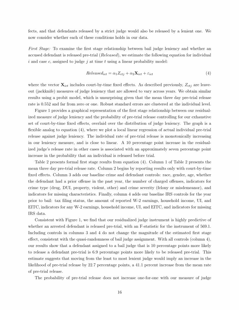
First Stage: To examine the first stage relationship between bail judge leniency and whether anaccused defendant is released pre-trial (Released), we estimate the following equation for individuali and case c, assigned to judge j at time t using a linear probability model:

Releasedict = α1Zctj + α2Xict + εict (4)

where the vector Xict includes court-by-time fixed effects. As described previously, Zctj are leave-out (jackknife) measures of judge leniency that are allowed to vary across years. We obtain similarresults using a probit model, which is unsurprising given that the mean three day pre-trial releaserate is 0.552 and far from zero or one. Robust standard errors are clustered at the individual level.

Figure 1 provides a graphical representation of the first stage relationship between our residual-ized measure of judge leniency and the probability of pre-trial release controlling for our exhaustiveset of court-by-time fixed effects, overlaid over the distribution of judge leniency. The graph is aflexible analog to equation (4), where we plot a local linear regression of actual individual pre-trialrelease against judge leniency. The individual rate of pre-trial release is monotonically increasingin our leniency measure, and is close to linear. A 10 percentage point increase in the residual-ized judge’s release rate in other cases is associated with an approximately seven percentage pointincrease in the probability that an individual is released before trial.

Table 2 presents formal first stage results from equation (4). Column 1 of Table 2 presents themean three day pre-trial release rate. Column 2 begins by reporting results only with court-by-timefixed effects. Column 3 adds our baseline crime and defendant controls: race, gender, age, whetherthe defendant had a prior offense in the past year, the number of charged offenses, indicators forcrime type (drug, DUI, property, violent, other) and crime severity (felony or misdemeanor), andindicators for missing characteristics. Finally, column 4 adds our baseline IRS controls for the yearprior to bail: tax filing status, the amount of reported W-2 earnings, household income, UI, andEITC, indicators for any W-2 earnings, household income, UI, and EITC, and indicators for missingIRS data.

Consistent with Figure 1, we find that our residualized judge instrument is highly predictive ofwhether an arrested defendant is released pre-trial, with an F-statistic for the instrument of 569.1.Including controls in columns 3 and 4 do not change the magnitude of the estimated first stageeffect, consistent with the quasi-randomness of bail judge assignment. With all controls (column 4),our results show that a defendant assigned to a bail judge that is 10 percentage points more likelyto release a defendant pre-trial is 6.9 percentage points more likely to be released pre-trial. Thisestimate suggests that moving from the least to most lenient judge would imply an increase in thelikelihood of pre-trial release by 22.7 percentage points, a 41.1 percent increase from the mean rateof pre-trial release.

The probability of pre-trial release does not increase one-for-one with our measure of judge

16

leniency, likely because of measurement error that attenuates the effect toward zero. For instance,judge leniency may drift over the course of the year or fluctuate with case characteristics, reducingthe accuracy of our leave-one-out measure. Nevertheless, the results from Figure 1 and Table 2confirm that judge leniency is highly predictive of detention outcomes in our setting.

Appendix Table 3 presents additional first stage results. We find that a defendant assigned to abail judge that is 10 percentage points more likely to release a defendant pre-trial is 4.0 percentagepoints less likely to petition for bail modification, 6.8 percentage points more likely to be releasedwithin 14 days of the bail hearing, and 5.7 percentage points more likely to ever be released beforetrial. These results indicate that the bail decision made by the first assigned bail judge is extremelypersistent.

Instrument Validity: Two additional conditions must hold to interpret our two-stage least squaresestimates as the local average treatment effect (LATE) of pre-trial release: (1) bail judge assignmentonly impacts defendant outcomes through the probability of pre-trial release, and (2) the impact ofjudge assignment on the probability of pre-trial release is monotonic across defendants.

Table 3 verifies that assignment of cases to bail judges is random after we condition on our court-by-time fixed effects. The first column of Table 3 uses a linear probability model to test whethercase and defendant characteristics are predictive of pre-trial release. These estimates capture bothdifferences in the bail conditions set by the bail judges and differences in these defendants’ abilityto meet the bail conditions. We control for court-by-time fixed effects and cluster standard errorsat the individual level. We find that male defendants are 11.4 percentage points less likely to bereleased pre-trial compared to similar female defendants, a 20.7 percent decrease from the meanpre-trial release rate of 55.2 percent. Black defendants are 3.9 percentage points less likely to bereleased compared to white defendants, a 7.1 percent decrease from the mean. Defendants witha prior offense in the past year are 15.3 percentage points less likely to be released compared todefendants with no prior offense, a 27.7 percent decrease. Additionally, defendants arrested forfelonies are 25.4 percentage points less likely to be released than those arrested for misdemeanors,a 46.0 percent decrease. Drug defendants are 11.9 percentage points more likely to be releasedcompared to defendants in the omitted category, and DUI defendants are 10.6 percentages pointsmore likely to be released. Violent defendants are 1.6 percentage points less likely to be releasedcompared to defendants in the omitted category, while property defendants are 0.9 percentage pointsmore likely to be released. Finally, individuals who are matched to IRS records, and defendantswith higher baseline earnings, UI benefits, EITC benefits, and baseline employment status are morelikely to be released pre-trial.

Column 2 assesses whether these same case and defendant characteristics are predictive of ourjudge leniency measure using an identical specification. We find evidence that bail judges of differingtendencies are assigned very similar defendants (joint p-value = 0.26), suggesting that the exclusionrestriction is valid in our setting.

Nevertheless, the exclusion restriction could also be violated if bail conditions imposed by judgeshad an independent effect on outcomes other than through the channel of pre-trial release. For exam-

17

ple, conditional on a defendant posting monetary bail, a higher bail amount may have independenteffects on outcomes. Note that in our setting, the exclusion restriction is more likely to be validthan in the context of using sentencing judge tendencies as an instrument for incarceration (Kling2006, Mueller-Smith 2015). In the context of sentencing, judges impose multiple treatments suchas incarceration, probation, and fines (Mueller-Smith 2015). In contrast, bail judges in our settingexclusively handle the setting of bail and a separate judge takes over the subsequent trial and sen-tencing processes. However, to the extent that the exclusion restriction is violated, our reduced formestimates can be interpreted as the causal impact of being assigned to a more or less lenient bailjudge. These reduced form results are available in Appendix Table 4. Our reduced form estimatesare very similar to the two-stage least estimates throughout, consistent with the strong first stagerelationship between the propensity of the assigned judge to release a defendant pre-trial and one’sown detention outcome.

The second condition needed to interpret our estimates as the LATE of pre-trial release is that theimpact of judge assignment on the probability of pre-trial release is monotonic across defendants. Inour setting, this monotonicity assumption requires that individuals released by a strict judge wouldalso be released by a more lenient judge, and similarly that individuals detained by a lenient judgewould also be detained by a stricter judge. One testable implication of the monotonicity assumptionis that the first stage estimates should be non-negative for all subsamples. Panel A of AppendixTable 5 and Appendix Table 6 present these first stage results using the full sample of cases tocalculate our measure of judge leniency. In all subsamples, we find that our residualized measure ofjudge leniency is consistently positive and sizable, in line with the monotonicity assumption.

A second implication of the monotonicity assumption is that judges who are stricter towardsone group (e.g., minority defendants) are also relatively strict towards other defendants outsideof this group (e.g., white defendants). Following Bhuller et al. (2016), we test this assumptionby estimating first stage results for all subsamples, but recalculate our judge leniency instrumentin each subsample using cases from the opposing subsample. Panel B of Appendix Table 5 andAppendix Table 6 present these results. In all subsamples, we find that our first stage estimatesusing this “reverse-sample instrument” are positive and statistically different from zero.

Appendix Figure 4 further explores how judges treat cases of observably different defendantsby plotting our residualized judge leniency measures calculated separately by race, offense type,offense severity, prior criminal history, and employment status. Each plot reports the coefficientand standard error from an OLS regression relating each measure of judge leniency. Consistentwith our monotonicity assumption, we find that the slopes relating the relationship between judgeleniency in one group and judge leniency in another group is non-negative, suggesting that judgetendencies are similar across observably different defendants and cases. We provide further evidencethat the monotonicity condition is satisfied in robustness checks.

18

IV. Results

In this section, we examine the effects of pre-trial release using the judge IV strategy describedabove. We first analyze the effects of pre-trial release on case outcomes, before turning to its effectson bail jumping, future crime, and labor market outcomes.

A. Case Outcomes

Table 4 presents OLS and two-stage least squares estimates of the impact of being released from jailwithin three days of the bail hearing on various case outcomes. Column 1 reports the dependentvariable mean for defendants who are detained pre-trial. Columns 2-4 report OLS estimates whereeach column further controls for potential omitted variables to learn about the source(s) and sizeof any bias. Column 2 begins by reporting results only with court-by-time fixed effects. Column3 adds our baseline crime and defendant controls: race, gender, age, whether the defendant had aprior offense in the past year, the number of charged offenses, indicators for crime type (drug, DUI,property, violent, other) and crime severity (felony or misdemeanor), and indicators for missingcharacteristics. Finally, column 4 adds our baseline IRS controls for the year prior to bail: tax filingstatus, the amount of reported W-2 earnings, household income, UI, and EITC, indicators for anyW-2 earnings, household income, UI, and EITC, and indicators for missing IRS data. Columns 5-7report analogous two-stage least squares results where we instrument for pre-trial release withinthree days using the leave-out measure of judge leniency described in Section III. Robust standarderrors clustered at the individual level are reported throughout.

The OLS estimates show that released defendants have significantly better case outcomes thandetained defendants. In all specifications, released defendants are significantly less likely to be foundguilty of an offense, to plead guilty to a charge, and to be incarcerated following case disposition.However, the magnitudes of these OLS estimates are extremely sensitive to the addition of baselinecrime controls. For example, in our OLS results with only our court-by-time fixed effects (column2), we find that a defendant who is released pre-trial is 18.6 percentage points less likely to pleadguilty, a 42.7 percent decrease from the mean for detained defendants. When we add baseline crimeand defendant controls (column 3), the magnitude of the estimate is more than halved, droppingto 9.2 percentage points. In contrast, adding baseline IRS controls (column 4) does not change thesize of the estimate, which remains at 9.2 percentage points. These results suggest that, at leastfor case outcomes, crime and defendant controls are important for addressing potential omittedvariable bias. Controls for baseline labor market outcomes appear relatively unimportant for thesecase outcomes.

The two-stage least squares estimates in columns 5-7 improve upon our OLS estimates by exploit-ing plausibly exogenous variation in pre-trial release from the quasi-random assignment of cases tobail judges. These two-stage least squares results confirm that defendants released before trial havesignificantly better case outcomes than otherwise similar defendants detained before trial. With thefull set of controls (column 7), we find that the marginal released defendant is 15.6 percentage points

19

less likely to be found guilty, a 27.3 percent decrease from the mean, and 12.0 percentage pointsless likely to plead guilty, a 27.5 percent decrease from the mean. These results are consistent withthe theory that pre-trial release improves a defendant’s bargaining position in plea negotiations. InAppendix Table 7, we find that marginal released defendants are also convicted of fewer offenses,more likely to be convicted of a lesser charge, and less likely to plead guilty to time served.

We find that the marginal released defendant is also 3.0 percentage points less likely to beincarcerated after case disposition, a 10.1 percent decrease from the mean, although the estimate isnot statistically significant. Large standard errors mean that the difference between the OLS andtwo-stage least squares estimates for incarceration is not statistically significant, however. In SectionIV.D, we find that the impact of pre-trial release on incarceration is large and statistically significantfor felony and drug defendants, cases with a much higher baseline rate of incarceration. These resultssuggest that pre-trial release reduces post-trial incarceration primarily for defendants charged withmore severe crimes, most likely through a reduction in the extensive margin of conviction ratherthan the intensive margin of punishment conditional on conviction.

To make the counterfactual more precise, we estimate results that differentiate between releasewithout any conditions (ROR) and release with conditions. By separately estimating these twodecision margins relative to detention, we can test whether our results are driven solely by a defen-dant being released before trial, or by some combination of pre-trial release and release conditionsimposed by the bail judge. Unfortunately, our data do not allow us to identify the specific conditionsof release, ranging from minimal requirements like reporting to a Pre-Trial Services officer to moreintensive conditions like electronic monitoring or home confinement.26

In Appendix Table 9, we present OLS and two-stage least squares estimates of the impact ofbeing released from jail within three days of the bail hearing with and without conditions. Whilethe OLS results suggest that pre-trial release improves case outcomes more for defendants who arereleased with no conditions relative to those who are released with conditions, the two-stage leastsquares estimates show no statistically significant differences in the effect of pre-trial release onmarginal defendants with and without conditions. For example, the marginal defendant releasedwith no conditions is 12.9 percentage points less likely to plead guilty and the marginal defendantreleased with conditions is 11.9 percentage points less likely to plead guilty. Our standard errorsare also precise enough that we can rule out any large differences by release type. These findingssuggest that pre-trial release by itself improves case outcomes.

B. Bail Jumping and Future Crime

The results described above suggest that there are significant costs of pre-trial detention for de-fendants. However, it is also possible that pre-trial detention benefits society by increasing courtappearances or by reducing bail jumping and future crime.

26In Appendix Table 8, we document a strong first stage relationship between a defendant’s pre-trial releaseconditions and the assigned judge’s propensity for release with or without conditions, with judges independentlyvarying across these two margins.

20

Table 5 examines the impact of pre-trial release on various procedural measures of court perfor-mance. We find that pre-trial release leads to substantial increases in failing to appear for requiredcourt appearances and fleeing from the jurisdiction.27 The OLS estimates show that released de-fendants are significantly more likely to miss a court appearance and jump bail. However, themagnitudes of these OLS estimates are extremely sensitive to the addition of baseline crime con-trols. For example, in our OLS results with only our court-by-time fixed effects (column 2), wefind that a defendant who is released pre-trial is 6.3 percentage points more likely to miss a courtappearance, a 52.1 percent decrease from the mean for detained defendants. When we add baselinecrime and defendant controls (column 3), the magnitude of the estimate drops to only 0.7 percent-age points. Adding baseline IRS controls (column 4) does not significantly change the size of theestimate.

Our two-stage least squares results also suggest that released defendants are more likely to misscourt appearances and jump bail. Controlling for our full set of controls (column 7), we find that themarginal released defendant is 15.0 percentage points more likely to fail to appear in court, a 124.0percent increase from the mean. Bail jumping also increases by 0.6 percentage points, a 300 percentincrease from the detained defendant mean, but the estimate is not statistically significant due tothe relative infrequency of this outcome. As before, we find no statistically significant differences inthe effect of pre-trial release on failures to appear for marginal defendants released with and withoutconditions (Appendix Table 9).

We also find that the marginal released defendant waits an extra 48.6 days between bail andcase disposition, a 24.3 percent increase from the mean. Increases in case disposition length maybe due to speedy trial rules in both Pennsylvania and Florida, which effectively place limits on howlong a defendant can be detained pre-trial.28 In addition, marginal released defendants may waitlonger between bail and case disposition because they are less likely to plead guilty.

Table 6 presents estimates of the impact of pre-trial release on future criminal behavior. Weexplore both short-run (mechanical) effects prior to case disposition and longer-term effects up tofour years after the bail hearing. For crime within two years, our sample is limited to the 306,634defendants who we observe for two years following the bail hearing, and for crime within four years,our sample is limited to the 202,166 defendants who we observe for four years following the bailhearing. We measure crime using rearrests, but the results follow a similar pattern if we use newconvictions instead.

Both with and without baseline controls, our OLS results show that released defendants aremore likely to be arrested before case disposition, but less likely to be arrested in future years. Forexample, with all baseline controls (column 4), we find that released defendants are 5.8 percentage

27These measures are only available in our Philadelphia sample.28In Pennsylvania, other than cases in which a defendant is not entitled to release on bail, a defendant generally

cannot be detained for longer than 180 days from the date the complaint is filed. In Florida, formal charges areusually filed within 21 days of arrest, and may not be delayed beyond 33 days. If charges have not been filed within33 days of arrest, any defendants who are detained will be released from custody ROR. In Florida, persons chargedwith felonies are entitled to be brought to trial within 175 days of having been taken into custody and persons chargedwith misdemeanors are entitled to be brought to trial within 90 days of having been taken into custody.

21

points more likely to be rearrested compared to a detained defendant, a 28.7 percent increase fromthe mean. These results are largely mechanical – it is impossible to be rearrested for a new crimewhen one is incapacitated. Nevertheless, these results suggest that released defendants are stillengaged in some criminal behavior before case disposition. In contrast, released defendants are 1.8percentage points less likely to be rearrested in the two years following the bail hearing, includingthe time period prior to case disposition. Similarly, released defendants are 4.7 percentage pointsless likely to be rearrested in the third to fourth years following the bail hearing. In contrast to thecase outcomes results, the OLS results are relatively insensitive to the addition of controls for crimecharacteristics or baseline labor market outcomes.

Our two-stage least squares results follow a similar pattern for arrests prior to case dispositionand in the first two years following the bail hearing. With all baseline controls (column 7), wefind that the marginal released defendant is 7.6 percentage points more likely to be rearrested fora new crime prior to disposition, a 37.6 percent increase from the mean, but 5.0 percentage pointsless likely to be arrested in the two years following the bail hearing. The point estimate for ourtwo year result is not statistically significant, however. In contrast to the OLS results, we find apositive but statistically insignificant point estimate on rearrest in the third to fourth years followingthe bail hearing. Taken together, we interpret these results as suggesting that pre-trial detentionprevents new criminal activity prior to case disposition through a short-run incapacitation effect,but has little net impact on future crime following case disposition. However, we emphasize thatfor longer-run measures of crime, the large standard errors and smaller sample size makes definitiveconclusions difficult. Finally, we again find that our results on future crime are similar for marginaldefendants who are released with and without conditions (Appendix Table 9).

C. Labor Market and Tax Administration Outcomes

Table 7 presents estimates of the impact of pre-trial release on individual-level formal sector earningsand employment. For outcomes measured as the average across the first two years post-bail hearing,our sample is limited to the 302,816 defendants matched to IRS data with cases before 2013, andfor outcomes measured as the average over the third to fourth years post-bail hearing, our sampleis limited to the 224,319 defendants matched to IRS data with cases before 2011.

The OLS estimates in Table 7 show that released defendants have significantly higher formalsector earnings and employment following the bail hearing. For example, with all baseline controls(column 4), released defendants are 5.1 percentage points more likely to be employed within twoyears of the bail hearing, a 13.5 percent increase from the mean, and 3.6 percentage points morelikely to have any income, a 7.8 percent increase from the mean. However, the magnitude ofthese OLS estimates are extremely sensitive to the addition of baseline labor market controls. Forexample, with no baseline controls (column 2), the OLS estimates suggest that released defendantsearn approximately $2,681 more per year than detained defendants in the two years following thebail hearing, a 51.5 percent increase from the mean. Adding baseline crime and defendant controlsdoes little to alter the significance and magnitude of these results (column 3). However, the estimate

22

falls to only $406 with the addition of the baseline IRS controls. The OLS results follow a similarpattern for formal sector earnings and employment in the third to fourth years following the bailhearing. These results imply that, perhaps not surprisingly, controlling for baseline earnings andemployment is critical when estimating the impact of pre-trial release on labor market outcomes.

The two-stage least squares estimates are broadly similar to the OLS estimates with baselinecontrols, but much less precisely estimated. With our full set of baseline controls (column 7), wefind that marginal released defendants are 9.7 percentage points more likely to have any income twoyears after bail, a 21.0 percent increase from the mean. Estimates on other outcomes in the first twoyears post-bail hearing are smaller and not statistically different from zero. By three to four yearspost-bail hearing, released defendants are 10.2 percentage points more likely to be employed in theformal labor sector, a 26.9 percent increase from the mean. Formal sector earnings are $1,024 higherover the same time period, a 17.5 percent increase from the mean, and the probability of having anyincome is 8.5 percentage points higher, a 18.3 percent increase from the mean. Although neither ofthese estimates are statistically significant, they are broadly consistent with the more precise OLSestimates with our full set of baseline controls (column 4). When we separately identify marginaldefendants who are released with and without conditions, we find no significant differences in theimpact of pre-trial release by release type (Appendix Table 9).29

Table 8 presents estimates for tax filing, UI receipt, and EITC receipt – measures of formal sectorengagement that are particularly welfare-relevant in our low-income population. For example, only30.8 percent of detained defendants file a tax return three to four years after the bail hearing, muchlower than would be typical for the average working-age adult. In our two-stage least squares resultswith the full set of controls (column 7), we find that released defendants are 9.5 percentage pointsmore likely to file a tax return one to two years post-bail, a 22.4 percent increase from the mean.Pre-trial release also increases the receipt of EITC benefits by $185 over the same time period, a55.4 percent increase. Three to four years post-bail, released defendants are 4.3 percentage pointsmore likely to file a tax return, a 14.0 percent increase from the mean, and receive an additional$323 in UI benefits and $239 in EITC benefits, 131.8 and 66.4 percent increases from the mean,respectively. These results suggest that pre-trial release allows individuals to remain connected tothe formal sector, both through employment in the formal labor market and the increased take-upof social benefits that are tied to formal sector employment.

D. Subsample Results

Table 9 presents selected two-stage least squares subsample results by crime severity and highestcrime type. We find that the effects on case outcomes are consistently larger for misdemeanor

29A valid question is why we find a significant impact of pre-trial release on the extensive margin, but insignificanteffects on the intensive margin. One possible explanation is that our intensive margin estimates are particularlynoisy due to the right-skewness of the income distribution among defendants in our sample. Consistent with thisexplanation, we find that total household income is significantly higher among marginal released defendants when wetop-code earnings at the 75th percentile of the earnings distribution in our sample. These results are available uponrequest from the authors.

23

offenses. For example, released misdemeanor defendants are 19.0 percentage points less likely tobe found guilty and 18.6 percentage points less likely to plead guilty. In contrast, released felonydefendants are only 10.0 percentage points less likely to be found guilty and 1.2 percentage pointsless likely to plead guilty. However, effects on incarceration are nearly 10 percentage points largerfor felony defendants, likely because the baseline rate of incarceration is nearly three times higherfor felonies compared to misdemeanors. Released felony defendants are also 9.4 percentage pointsmore likely to miss a court appearance compared to released misdemeanor defendants, potentiallybecause felony defendants have a higher flight risk. Effects for other outcomes are largely similarfor the two groups.

By crime type, case outcomes are most precisely estimated for drug and property defendants.For example, released drug defendants are 10.8 percentage points less likely to be found guiltyand 12.8 percentage points less likely to be incarcerated. Released property defendants are 14.3percentage points less likely to be found guilty and 10.7 percentage points less likely to plead guilty.However, the point estimates for nearly all outcomes, particularly labor market outcomes, are largerfor defendants charged with violent offenses, although large standard errors mean that few of theestimates are statistically significant. With that caveat, it is possible that the larger labor marketeffects for violent offenders are due to the greater stigma associated with a conviction for a violentoffense (Holzer et al. 2003).

Table 10 presents additional subsample results by defendant race, prior criminal history, andbaseline employment status. We find that for nearly all outcomes, our estimates are larger forwhite defendants compared to black defendants. For example, released white defendants are 25.9percentage points less likely to be found guilty and 19.8 percentage points less likely to plead guilty,compared to only 10.1 percentage points and 12.2 percentage points less likely for released blackdefendants. Released white defendants are also more likely to be rearrested prior to dispositionthan released black defendants. Finally, we find that released white defendants are substantiallymore likely to have any income several years post-bail compared to released black defendants.

By criminal history, we find that the impacts of pre-trial release are largest for those without aprior offense in the past year. For individuals without a recent prior offense, released defendants are20.2 percentage points less likely to be found guilty, 15.2 percentage points less likely to plead guilty,and 10.7 percentage points more likely to be employed three to four years post-bail. In contrast,almost all results for individuals with a recent prior offense are small and imprecisely estimated.These results suggest that the social costs imposed by pre-trial detention are relatively larger forthose with more limited ties to the criminal justice system.

We also find suggestive evidence that pre-trial release improves case outcomes the most fordefendants who were employed in the year prior to bail. For example, among those employedprior to the bail hearing, released defendants are 18.5 percentage points less likely to be foundguilty, 10.9 percentage points less likely to plead guilty, and 7.3 percentage points less likely to beincarcerated. In contrast, among those not employed prior to the bail hearing, released defendantsare 10.3 percentage points less likely to be found guilty, 10.7 percentage points less likely to plead

24

guilty, and 2.0 percentage points less likely to be incarcerated. While not precisely estimated, ourlabor market results are also larger for individuals who were employed prior to bail. Overall, theseresults suggest that pre-trial detention imposes relatively larger costs on individuals with strongerties to the formal labor sector.

E. Robustness Checks

Appendix Table 10 explores the sensitivity of our main results to alternative specifications. Column1 uses a leave-out measure of judge leniency that is allowed to differ for misdemeanors and felonies,thereby relaxing the monotonicity assumption. Column 2 uses a leave-out measure that is allowedto differ for the five mutually exclusive crime types – drug, violent, DUI, property, and other –again relaxing the monotonicity assumption. Column 3 estimates results on whether the defendantis ever released pre-trial, and column 4 estimates results on whether the defendant is assigned non-monetary bail. Column 5 uses a randomly selected subset of 25 percent of cases to calculate aleave-out measure of judge leniency that is used as an instrument in the mutually exclusive subsetof cases. Column 6 calculates judge leniency based on the scheduled bail judge, which differs fromthe assigned bail judge approximately 30 percent of the time, and column 7 presents results using afull set of judge fixed effects as instruments. Appendix Table 11 presents our main results separatelyfor Philadelphia (column 1), Miami-Dade (column 2), and the sample matched to the IRS (column3). Results across all specifications are similar to our preferred specification. None of the estimatessuggest that our preferred estimates are invalid.

V. Discussion

In this section, we tentatively explore the potential mechanisms that might explain our findings oncase and labor market outcomes.

Case Outcomes: Pre-trial release could improve case outcomes through at least two main channels.First, pre-trial release may strengthen a defendant’s bargaining position during plea negotiations.For example, it is possible that pre-trial release decreases a defendant’s incentive to plead guilty toobtain a faster release from jail. Along the same lines, it is also possible that pre-trial release affectsa defendant’s ability to prepare an adequate defense or negotiate a settlement with prosecutors. Thesecond reason that pre-trial release could impact conviction rates is that seeing detained defendantsin jail uniforms and shackles may bias judges or jurors at trial. For example, jurors may assumethat only guilty defendants are detained before trial.

While there is no conclusive evidence on this issue, two pieces of evidence suggest that our resultsare likely driven by changes in a defendant’s bargaining position. First, as discussed previously, wefind that released defendants are substantially less likely to be convicted of any offense due to areduction in guilty pleas, not changes in conviction rates at trial where jury bias may come intoplay. Second, we find that those who are released pre-trial receive more favorable plea deals thanthose who are detained. For example, we find that released defendants are substantially more likely

25

to be convicted of a lesser charge and are convicted of fewer total offenses (Appendix Table 7). Thefact that so many of our results are driven by changes at the plea bargaining phase, and not the trialphase, suggests that pre-trial release improves case outcomes primarily through a strengthening ofdefendants’ bargaining positions.

Labor Market Outcomes: Pre-trial release could improve labor market outcomes through at leastthree main channels. First, pre-trial release might increase labor market attachment through amechanical incapacitation effect since defendants cannot work in the formal sector while detainedor incarcerated post-conviction. Defendants who are imprisoned are also ineligible to claim UIbenefits and EITC benefits for wages earned while incarcerated. Second, pre-trial release mightimprove outcomes because detention is highly disruptive to defendants’ lives, potentially leading tojob loss, which makes it harder for defendants to find new employment. Finally, pre-trial detentioncould independently lower future employment prospects through the stigma of a criminal conviction(e.g. Mueller-Smith 2015, Agan and Starr 2016), which could in turn limit defendants’ eligibilityfor employment-related benefits like UI and EITC.

We view our results as being inconsistent with the incapacitation channel. For example, we findthat pre-trial release increases formal labor market employment in the three to four years post-bail,but the average sentence length in our sample is only 186 days. Among misdemeanor offenses, theaverage sentence length is 30 days, yet we continue to find suggestive evidence of increased labormarket attachment several years post-bail.

To partially test whether pre-trial release improves labor market outcomes through the criminalconviction channel, we explore whether those who are more likely to be employed in the labor marketare also those who do not have a criminal conviction. In Appendix Table 12, we present estimatesof the joint probability of conviction and employment in the several years post-bail. We find thatin the first two years after the bail hearing, our main employment results are primarily driven byan increase in the joint probability of not having a criminal conviction and being employed in theformal labor market. By the third to fourth years after the bail hearing, our employment estimatesare entirely driven by the joint probability of having no criminal conviction and being employed.We conclude from these results that pre-trial release primarily affects future labor market outcomesthrough the channel of a criminal conviction.

VI. Conclusion

This paper estimates the impact of being released before trial on criminal case outcomes, futurecrime, formal sector employment, and the receipt of government benefits. We find that pre-trialrelease significantly decreases the probability of conviction, primarily through a decrease in guiltypleas. Pre-trial release mechanically increases pre-trial crime and failures to appear in court, buthas no detectable effect on future crime. Finally, we find suggestive evidence that pre-trial releaseincreases formal sector attachment both through an increase in formal sector employment and thereceipt of tax- and employment-related government benefits. Many of the estimated effects are

26

larger for defendants with no prior offenses in the past year and defendants employed in the yearprior to bail. We argue that these results are consistent with (i) pre-trial release strengtheningdefendants’ bargaining position during plea negotiations, and (ii) a criminal conviction loweringdefendants’ attachment to the formal labor market.

Our results suggest that it may be welfare enhancing to use alternatives to pre-trial detention,at least on the margin. For example, Di Tella and Schargrodsky (2013) find that recidivism ratesare substantially lower among individuals who randomly receive electronic monitoring compared todetention. Electronic monitoring is also extremely cost-effective compared to jail, with the annualcost of electronic monitoring in the United States at roughly $3,650 compared to over $30,000 forincarceration. To the extent that their results extend to our setting, electronic monitoring couldprovide many of the same benefits of pre-trial detention without the substantial costs to defendantsdocumented in our analysis.

In addition, our results offer important lessons for tax administration and policy related toindividuals who interact with the criminal justice system. As described above, we find that criminaldefendants are substantially more likely to file a tax return and to claim the EITC in subsequentyears if they are released pre-trial. One possible explanation is that pre-trial release raises thelikelihood of formal sector employment, which is a prerequisite for claiming the EITC. In turn,eligibility for the EITC may greatly increase the incentives for individuals to file tax returns. Anotherexplanation is that pre-trial release may contribute to tax filing and benefit take-up by improving(all else equal) defendants’ attitudes towards the government. These findings suggest that bailreform and outreach to those with criminal convictions may be useful methods for increasing taxfiling and the take-up of social benefits.

There are at least three caveats to our analysis. First, we are unable to estimate the deterrenteffects of a more or less strict bail system. If a more strict bail system has a large deterrent effect,our analysis will understate the benefits of a harsher bail judge. Second, we are unable to measurethe impacts of pre-trial detention on informal sector earnings or consumption. If lost formal sectorearnings are largely replaced by informal earnings, the case against pre-trial detention is perhapsweaker. Finally, we are unable to draw any sharp welfare conclusions about the optimality of thecurrent bail system using our research design. The substantial costs of the bail system documentedin our analysis must be weighed against the social benefits of increasing court appearances anddecreasing pre-trial crime. While beyond the scope of this paper, developing a framework to assessthe welfare effects of the bail system is an important area of future work.

27

References

[1] Abrams, David S., Marianne Bertrand, and Sendhil Mullainathan. 2012. “Do Judges Vary inTheir Treatment of Race?” Journal of Legal Studies, 41(2): 347-383.

[2] Agan, Amanda Y., and Sonja B. Starr. 2016. “Ban the Box, Criminal Records, and StatisticalDiscrimination: A Field Experiment.” University of Michigan Law & Econ Research PaperNo. 16-012.

[3] Aizer, Anna, and Joseph Doyle, Jr. 2015. “Juvenile Incarceration, Human Capital, and Fu-ture Crime: Evidence from Randomly-Assigned Judges.” Quarterly Journal of Economics,130(2): 759-803.

[4] Alesina, Alberto, and Eliana La Ferrara. 2014. “A Test of Racial Bias in Capital Sentencing.”American Economic Review, 104(11): 3397-3433.

[5] Anwar, Shamena, Patrick Bayer, and Randi Hjalmarsson. 2012. “The Impact of Jury Race inCriminal Trials.” Quarterly Journal of Economics, 127(2): 1017-1055.

[6] Ares, Charles E., and Anne Rankin, and Herbert Sturz. 1963. “The Manhattan Bail Project:An Interim Report on the Use of Pre-trial Parole.” New York University Law Review 38(1):67-95.

[7] Autor, David, Andreas Ravndal Kostol, and Magne Mogstad. 2015. “Disability Benefits, Con-sumption Insurance, and Household Labor Supply.” MIT Working Paper.

[8] Ayres, Ian, and Joel Waldfogel. 1994. “A Market Test for Race Discrimination in Bail Setting.”Stanford Law Review, 46(5): 987-1047.

[9] Bhuller, Manudeep, Gordon B. Dahl, Katrine V. Loken, and Magne Mogstad. 2016. “Incarcer-ation, Recidivism and Employment.” Unpublished Working Paper.

[10] Bushway, Shawn D., and Jonah B. Gelbach. 2011. “Testing for Racial Discrimination in BailSetting Using Nonparametric Estimation of a Parametric Model.” Unpublished WorkingPaper.

[11] Chang, Tom, and Antoinette Schoar. 2008. “Judge Specific Differences in Chapter 11 and FirmOutcomes.” Unpublished Working Paper.

[12] Chetty, Raj, John N. Friedman, and Jonah Rockoff. 2014. “Measuring the Impacts of TeachersI: Evaluating Bias in Teacher Value-Added Estimates.” American Economic Review, 104(9):2593-2632.

[13] Clarke, Stevens H., Jean L. Freeman, and Gary G. Koch. 1976. “Bail Risk: A MultivariateAnalysis.” Journal of Legal Studies, 5(2):341-385.

[14] Cohen, Thomas H., and Brian A. Reaves. 2007. “State Court Processing Statistics, 1990-2004:Pretrial Release of Felony Defendants in State Courts.” Washington, DC: U.S. Departmentof Justice.

28

[15] Dahl, Gordon B., Andreas Ravndal Kostol, and Magne Mogstad. 2014. “Family Welfare Cul-tures.” Quarterly Journal of Economics, 129 (4): 1711-1752.

[16] Di Tella, Rafael, and Ernesto Schargrodsky. 2013. “Criminal Recidivism after Prison and Elec-tronic Monitoring.” Journal of Political Economy, 121(1): 28-73.

[17] Dobbie, Will, Paul Goldsmith-Pinkham, and Crystal Yang. 2015. “Consumer Bankruptcy andFinancial Health.” NBER Working Paper No. 21032.

[18] Dobbie, Will, and Jae Song. 2015. “Debt Relief and Debtor Outcomes: Measuring the Effectsof Consumer Bankruptcy Protection.” American Economic Review, 105(3): 1272-1311.

[19] Doyle, Joseph. 2007. “Child Protection and Child Outcomes: Measuring the Effects of FosterCare.” American Economic Review, 97(5): 1583-1610.

[20] Doyle, Joseph. 2008. “Child Protection and Adult Crime: Using Investigator Assignment toEstimate Causal Effects of Foster Care.” Journal of Political Economy, 116(4): 746-770.

[21] Durose, Matthew R., and Patrick A. Langan. 2007. “Felony Sentences in State Courts, 2004.”Bureau of Justice Statistics.

[22] French, Eric, and Jae Song. 2014. “The Effect of Disability Insurance Receipt on Labor Supply.”American Economic Journal: Economic Policy, 6(2): 291-337.

[23] Foote, Caleb. 1954. “Compelling Appearance in Court: Administration of Bail in Philadelphia.”University of Pennsylvania Law Review, 102: 1031-1079.

[24] Goldkamp, J. S. 1980. “The Effects of Detention on Judicial Decisions: A Closer Look.” JusticeSystem Journal, 5: 234-257.

[25] Goldkamp, J. S., and M.R. Gottfredson. 1988. “Development of Bail/Pretrial Release Guidelinesin Maricopa County Superior Court, Dade County Circuit Court and Boston MunicipalCourt. Washington, D.C.:National Institute of Justice.

[26] Gupta, Arpit, Christopher Hansman, and Ethan Frenchman. 2016. “The Heavy Costs of HighBail: Evidence from Judge Randomization.” Unpublished Working Paper.

[27] Holzer, Harry, Steven Raphael, and Michael Stoll. 2003. “Employer Demand for Ex-Offenders:Recent Evidence from Los Angeles.” Unpublished Working Paper.

[28] Kling, Jeffrey. 2006. “Incarceration Length, Employment, and Earnings.” American EconomicReview, 96(3): 863-876.

[29] Landes, William M. 1973. “The Bail System: An Economic Approach.” Journal of Legal Studies,2: 79-105.

[30] Leslie, Emily, and Nolan G. Pope. 2016. “The Unintended Impact of Pretrial Detention on CaseOutcomes: Evidence from NYC Arraignments.” Unpublished Working Paper.

[31] Maestas, Nicole, Kathleen Mullen, and Alexander Strand. 2013. “Does Disability InsuranceReceipt Discourage Work? Using Examiner Assignment to Estimate Causal Effects of SSDIReceipt.” American Economic Review, 103(5): 1797-1829.

29

[32] McIntyre, Frank, and Shima Baradaran. 2013. “Race, Prediction, and Pretrial Detention.”Journal of Empirical Legal Studies, 10(4): 741-770.

[33] Mueller-Smith, Michael. 2015. “The Criminal and Labor Market Impacts of Incarceration.”Unpublished Working Paper.

[34] Myers, Samuel L., Jr. 1981. “The Economics of Bail Jumping.” Journal of Legal Studies,10(2):381-396.

[35] Oleson, James C., Christopher T. Lowenkamp, John Wooldredge, Marie VanNostrand, andTimothy P. Cadigan. 2014. “The Sentencing Consequences of Federal Pretrial Supervision.”Crime & Delinquency: 1-21.

[36] Pager, Devah. 2003. “The Mark of a Criminal Record.” American Journal of Sociology, 108:937-975.

[37] Phillips, Mary T. 2008. “Bail, Detention, and Felony Case Outcomes.” New York CriminalJustice Agency, Inc.

[38] Reaves, Brian A. 2013. “Felony Defendants in Large Urban Counties, 2009 - Statistical Tables.”Washington, DC: U.S. Department of Justice.

[39] Rehavi, M. Marit, and Sonja B. Starr. 2014. “Racial Disparity in Federal Criminal Sentences.”Journal of Political Economy, 122(6): 1320-1354.

[40] Shubik-Richards, Claire and Don Stemen. 2010. “Philadelphia’s Crowded, Costly Jails: TheSearch for Safe Solutions.” Technical Report, Pew Charitable Trusts Philadelphia ResearchInitiative.

[41] Stevenson, Megan. 2016. “Distortion of Justice: How the Inability to Pay Bail Affects CaseOutcomes.” Unpublished Working Paper.

[42] Walmsley, Roy. 2013. “World Prison Population List (tenth edition),” International Centre forPrison Studies, London, United Kingdom.

[43] Western, Bruce. 2006. Punishment and Inequality in America. New York: Russell Sage Foun-dation.

[44] Williams, Marian R. 2003. “The Effect of Pretrial Detention on Imprisonment Decisions.” Crim-inal Justice Review, 28: 299-316.

30

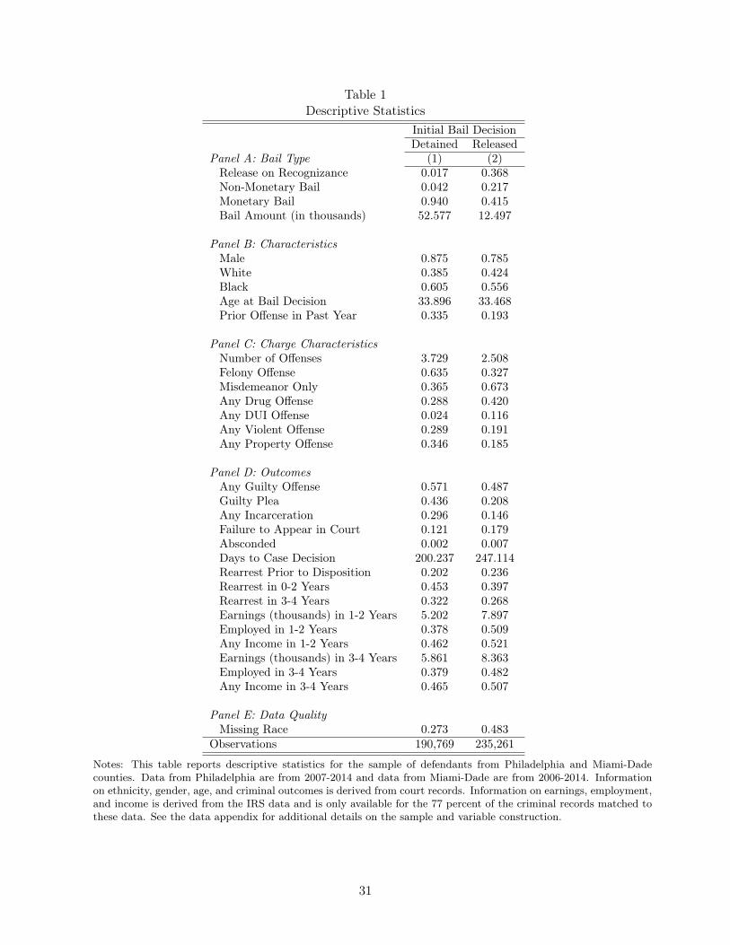
Table 1Descriptive Statistics

Initial Bail DecisionDetained Released

Panel A: Bail Type (1) (2)Release on Recognizance 0.017 0.368Non-Monetary Bail 0.042 0.217Monetary Bail 0.940 0.415Bail Amount (in thousands) 52.577 12.497

Panel B: CharacteristicsMale 0.875 0.785White 0.385 0.424Black 0.605 0.556Age at Bail Decision 33.896 33.468Prior Offense in Past Year 0.335 0.193

Panel C: Charge CharacteristicsNumber of Offenses 3.729 2.508Felony Offense 0.635 0.327Misdemeanor Only 0.365 0.673Any Drug Offense 0.288 0.420Any DUI Offense 0.024 0.116Any Violent Offense 0.289 0.191Any Property Offense 0.346 0.185

Panel D: OutcomesAny Guilty Offense 0.571 0.487Guilty Plea 0.436 0.208Any Incarceration 0.296 0.146Failure to Appear in Court 0.121 0.179Absconded 0.002 0.007Days to Case Decision 200.237 247.114Rearrest Prior to Disposition 0.202 0.236Rearrest in 0-2 Years 0.453 0.397Rearrest in 3-4 Years 0.322 0.268Earnings (thousands) in 1-2 Years 5.202 7.897Employed in 1-2 Years 0.378 0.509Any Income in 1-2 Years 0.462 0.521Earnings (thousands) in 3-4 Years 5.861 8.363Employed in 3-4 Years 0.379 0.482Any Income in 3-4 Years 0.465 0.507

Panel E: Data QualityMissing Race 0.273 0.483

Observations 190,769 235,261

Notes: This table reports descriptive statistics for the sample of defendants from Philadelphia and Miami-Dadecounties. Data from Philadelphia are from 2007-2014 and data from Miami-Dade are from 2006-2014. Informationon ethnicity, gender, age, and criminal outcomes is derived from court records. Information on earnings, employment,and income is derived from the IRS data and is only available for the 77 percent of the criminal records matched tothese data. See the data appendix for additional details on the sample and variable construction.

31

Table 2Judge Leniency and Pre-Trial Release

SampleMean Judge Leniency(1) (2) (3) (4)

Pre-Trial Release 0.552 0.693∗∗∗ 0.690∗∗∗ 0.687∗∗∗

(0.497) (0.025) (0.023) (0.023)Court x Year FE – Yes Yes YesCrime Controls – No Yes YesIRS Controls – No No YesObservations 426,030 426,030 426,030 426,030

Notes: This table reports first stage results. The regressions are estimated on the sample as described in the notes toTable 1. Judge leniency is estimated using data from other cases assigned to a bail judge in the same year followingthe procedure described in Section III. The dependent variable is an indicator for being released before trial withinthree days of the bail hearing. Column 1 reports the mean and standard deviation of the dependent variable. Column2 reports results controlling for our full set of court-by-time fixed effects. Column 3 adds crime and defendant baselinecontrols: defendant race, defendant gender, defendant age, whether the defendant had a prior offense with the pastyear, number of offenses, indicators for whether the defendant is arrested for a drug, DUI, violent, or propertyoffense, whether the most serious offense is a felony, and indicators for missing characteristics. Column 4 adds afull set of baseline IRS controls: whether the defendant was matched to the IRS data, baseline individual wages,baseline household wages, baseline UI, baseline EITC, baseline tax filing status, baseline employment, baseline anyUI, baseline any EITC, baseline any income, and indicators for missing income data. Robust standard errors clusteredat the individual level are reported in parentheses. *** = significant at 1 percent level, ** = significant at 5 percentlevel, * = significant at 10 percent level.

32

Table 3Test of Randomization

Pre-Trial JudgeRelease Leniency(1) (2)

Male −0.11385∗∗∗ −0.00003(0.00199) (0.00013)

Black −0.03922∗∗∗ 0.00005(0.00194) (0.00015)

Age at Bail Decision −0.01197∗∗∗ −0.00006(0.00065) (0.00005)

Prior Offense in Past Year −0.15286∗∗∗ 0.00010(0.00164) (0.00011)

Number of Offenses −0.02469∗∗∗ −0.00001(0.00032) (0.00002)

Felony Offense −0.25377∗∗∗ 0.00011(0.00198) (0.00010)

Any Drug Offense 0.11910∗∗∗ 0.00014(0.00192) (0.00013)

Any DUI Offense 0.10627∗∗∗ 0.00022(0.00261) (0.00015)

Any Violent Offense −0.01563∗∗∗ 0.00013(0.00226) (0.00015)

Any Property Offense 0.00832∗∗∗ −0.00027∗

(0.00201) (0.00015)Matched to IRS Data 0.00759∗∗∗ −0.00004

(0.00208) (0.00014)Baseline Earnings 0.00112∗∗∗ −0.00001

(0.00008) (0.00001)Baseline UI 0.00287∗∗∗ −0.00002

(0.00042) (0.00002)Baseline EITC 0.01187∗∗∗ 0.00002

(0.00102) (0.00007)Baseline Filed Return 0.04826∗∗∗ −0.00018

(0.00252) (0.00019)Baseline Employed 0.02529∗∗∗ 0.00015

(0.00205) (0.00015)Baseline Any EITC −0.01631∗∗∗ 0.00006

(0.00347) (0.00026)Baseline Any Income 0.00000 0.00000

(0.00000) (0.00000)Baseline Any UI 0.02333∗∗∗ 0.00032

(0.00396) (0.00026)Joint F-Test [0.00000] [0.26686]Observations 426,030 426,030

Notes: This table reports reduced form results testing the random assignment of cases to bail judges. Judge leniencyis estimated using data from other cases assigned to a bail judge in the same year following the procedure describedin Section III. Column 1 reports estimates from an OLS regression of pre-trial release on the variables listed andcourt-by-time fixed effects. Column 2 reports estimates from an OLS regression of judge leniency on the variableslisted and court-by-time fixed effects. The p-value reported at the bottom of columns 1-2 is for a F-test of the jointsignificance of the variables listed in the rows. Robust standard errors clustered at the individual level are reportedin parentheses in all specifications. *** = significant at 1 percent level, ** = significant at 5 percent level, * =significant at 10 percent level. See the data appendix for additional details on the sample and variable construction.

33

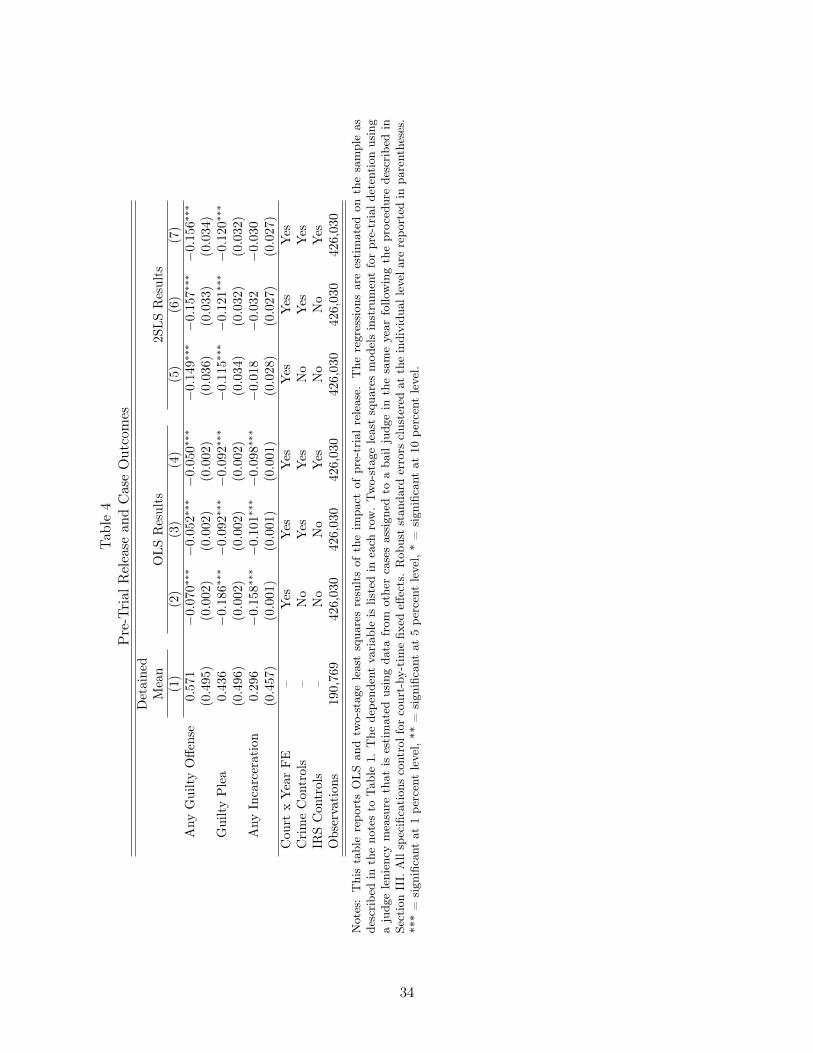
Tab

le4

Pre-Trial

Release

andCaseOutcomes

Detained

Mean

OLS

Results

2SLS

Results

(1)

(2)

(3)

(4)

(5)

(6)

(7)

Any

GuiltyOffe

nse

0.571

−0.07

0∗∗∗

−0.05

2∗∗∗

−0.05

0∗∗∗

−0.149∗

∗∗−0.15

7∗∗∗

−0.15

6∗∗∗

(0.495)

(0.002

)(0.002

)(0.002

)(0.036

)(0.033

)(0.034

)GuiltyPlea

0.436

−0.18

6∗∗∗

−0.09

2∗∗∗

−0.09

2∗∗∗

−0.115∗

∗∗−0.12

1∗∗∗

−0.12

0∗∗∗

(0.496

)(0.002

)(0.002

)(0.002

)(0.034)

(0.032

)(0.032

)Any

Incarceration

0.296

−0.15

8∗∗∗

−0.10

1∗∗∗

−0.09

8∗∗∗

−0.018

−0.03

2−0.03

0(0.457

)(0.001

)(0.001

)(0.001

)(0.028

)(0.027

)(0.027

)Cou

rtxYearFE

–Yes

Yes

Yes

Yes

Yes

Yes

CrimeCon

trols

–No

Yes

Yes

No

Yes

Yes

IRSCon

trols

–No

No

Yes

No

No

Yes

Observation

s190,769

426,030

426,030

426,030

426,03

042

6,03

042

6,03

0

Notes:Thistablerepo

rtsOLSan

dtw

o-stag

eleastsqua

resresultsof

theim

pact

ofpre-trialrelease.

The

regression

sareestimated

onthesampleas

describe

din

theno

testo

Tab

le1.

The

depe

ndentvariab

leis

listedin

each

row.Two-stag

eleastsqua

resmod

elsinstrumentforpre-trialde

tentionusing

ajudg

elenien

cymeasure

that

isestimated

usingda

tafrom

othe

rcasesassign

edto

aba

iljudg

ein

thesameyear

follo

wingtheproced

urede

scribe

din

SectionIII.Allspecification

scontrolfor

court-by

-tim

efix

edeff

ects.Rob

uststan

dard

errors

clusteredat

theindividu

allevela

rerepo

rted

inpa

renthe

ses.

***=

sign

ificant

at1pe

rcentlevel,**

=sign

ificant

at5pe

rcentlevel,*=

sign

ificant

at10

percentlevel.

34

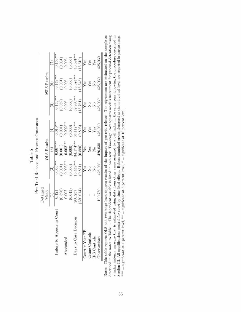
Tab

le5

Pre-Trial

Release

andProcess

Outcomes

Detained

Mean

OLS

Results

2SLS

Results

(1)

(2)

(3)

(4)

(5)

(6)

(7)

Failu

reto

App

earin

Cou

rt0.12

10.06

3∗∗∗

0.00

7∗∗∗

0.01

0∗∗∗

0.15

3∗∗∗

0.14

9∗∗∗

0.15

0∗∗∗

(0.326

)(0.001

)(0.001

)(0.001

)(0.032

)(0.031

)(0.031

)Abscond

ed0.00

20.00

5∗∗∗

0.00

2∗∗∗

0.00

2∗∗∗

0.00

60.00

60.00

6(0.045

)(0.000

)(0.000

)(0.000

)(0.006

)(0.006

)(0.006

)Daysto

CaseDecision

200.23

713.449

∗∗∗

34.174

∗∗∗

34.117

∗∗∗

52.980

∗∗∗

48.674

∗∗∗

48.591

∗∗∗

(250.014

)(0.851

)(0.886

)(0.895

)(15.76

1)(15.54

3)(15.61

0)Cou

rtxYearFE

–Yes

Yes

Yes

Yes

Yes

Yes

CrimeCon

trols

–No

Yes

Yes

No

Yes

Yes

IRSCon

trols

–No

No

Yes

No

No

Yes

Observation

s190,769

426,030

426,030

426,030

426,03

042

6,03

042

6,03

0

Notes:Thistablerepo

rtsOLSan

dtw

o-stag

eleastsqua

resresultsof

theim

pact

ofpre-trialrelease.

The

regression

sareestimated

onthesampleas

describe

din

theno

testo

Tab

le1.

The

depe

ndentvariab

leis

listedin

each

row.Two-stag

eleastsqua

resmod

elsinstrumentforpre-trialde

tentionusing

ajudg

elenien

cymeasure

that

isestimated

usingda

tafrom

othe

rcasesassign

edto

aba

iljudg

ein

thesameyear

follo

wingtheproced

urede

scribe

din

SectionIII.Allspecification

scontrolfor

court-by

-tim

efix

edeff

ects.Rob

uststan

dard

errors

clusteredat

theindividu

allevela

rerepo

rted

inpa

renthe

ses.

***=

sign

ificant

at1pe

rcentlevel,**

=sign

ificant

at5pe

rcentlevel,*=

sign

ificant

at10

percentlevel.

35

Tab

le6

Pre-Trial

Release

andFu

ture

Crime

Detained

Mean

OLS

Results

2SLS

Results

(1)

(2)

(3)

(4)

(5)

(6)

(7)

RearrestPrior

toDispo

sition

0.20

20.04

2∗∗∗

0.05

5∗∗∗

0.05

8∗∗∗

0.07

7∗∗

0.07

4∗∗

0.07

6∗∗

(0.402

)(0.001

)(0.001

)(0.001

)(0.033

)(0.033

)(0.033

)Rearrestin

0-2Years

0.45

3−0.04

9∗∗∗

−0.02

5∗∗∗

−0.01

8∗∗∗

−0.05

6−0.05

4−0.05

0(0.498

)(0.002

)(0.002

)(0.002

)(0.049

)(0.048

)(0.047

)Rearrestin

3-4Years

0.32

2−0.06

0∗∗∗

−0.05

3∗∗∗

−0.04

7∗∗∗

0.05

90.06

10.06

3(0.467

)(0.002

)(0.002

)(0.002

)(0.053

)(0.054

)(0.054

)Cou

rtxYearFE

–Yes

Yes

Yes

Yes

Yes

Yes

CrimeCon

trols

–No

Yes

Yes

No

Yes

Yes

IRSCon

trols

–No

No

Yes

No

No

Yes

Observation

s190,769

426,030

426,030

426,030

426,03

042

6,03

042

6,03

0

Notes:Thistablerepo

rtsOLSan

dtw

o-stag

eleastsqua

resresultsof

theim

pact

ofpre-trialrelease.

The

regression

sareestimated

onthesampleas

describe

din

theno

testo

Tab

le1.

The

depe

ndentvariab

leis

listedin

each

row.Two-stag

eleastsqua

resmod

elsinstrumentforpre-trialde

tentionusing

ajudg

elenien

cymeasure

that

isestimated

usingda

tafrom

othe

rcasesassign

edto

aba

iljudg

ein

thesameyear

follo

wingtheproced

urede

scribe

din

SectionIII.Allspecification

scontrolfor

court-by

-tim

efix

edeff

ects.Rob

uststan

dard

errors

clusteredat

theindividu

allevela

rerepo

rted

inpa

renthe

ses.

***=

sign

ificant

at1pe

rcentlevel,**

=sign

ificant

at5pe

rcentlevel,*=

sign

ificant

at10

percentlevel.

36

Tab

le7

Pre-Trial

Release

andLa

borMarketOutcomes

Detained

Mean

OLS

Results

2SLS

Results

Pan

elA

:Yea

rs1-

2(1)

(2)

(3)

(4)

(5)

(6)

(7)

Employed

0.37

80.13

4∗∗∗

0.10

2∗∗∗

0.05

1∗∗∗

0.07

30.06

80.03

7(0.485

)(0.002

)(0.002

)(0.002

)(0.049

)(0.049

)(0.043

)Any

Income

0.46

20.10

3∗∗∗

0.08

0∗∗∗

0.03

6∗∗∗

0.13

1∗∗∗

0.12

5∗∗∗

0.09

7∗∗

(0.499

)(0.002

)(0.002

)(0.002

)(0.048

)(0.048

)(0.045

)Earning

s(tho

usan

ds)

5.20

22.68

1∗∗∗

2.23

9∗∗∗

0.40

6∗∗∗

0.46

10.79

3−0.46

2(15.10

8)(0.071

)(0.073

)(0.044

)(1.536

)(1.539

)(0.976

)Hou

seho

ldIncome(tho

usan

ds)

10.215

2.68

9∗∗∗

2.19

1∗∗∗

0.24

1∗∗∗

2.25

02.77

0−0.25

1(22.74

1)(0.105

)(0.107

)(0.065

)(2.214

)(2.228

)(1.532

)

Pan

elB:Yea

rs3-

4Employed

0.37

90.10

3∗∗∗

0.07

7∗∗∗

0.03

2∗∗∗

0.11

1∗0.11

8∗∗

0.10

2∗

(0.485

)(0.002

)(0.003

)(0.002

)(0.057

)(0.058

)(0.053

)Any

Income

0.46

50.08

9∗∗∗

0.06

6∗∗∗

0.03

0∗∗∗

0.11

2∗∗

0.11

0∗0.08

5(0.499

)(0.002

)(0.003

)(0.002

)(0.055

)(0.057

)(0.054

)Earning

s(tho

usan

ds)

5.86

12.41

6∗∗∗

1.99

5∗∗∗

0.22

4∗∗∗

0.33

41.14

21.02

4(15.80

6)(0.085

)(0.088

)(0.061

)(1.858

)(1.898

)(1.338

)Hou

seho

ldIncome(tho

usan

ds)

10.953

2.43

4∗∗∗

1.94

6∗∗∗

0.03

61.25

92.08

5−0.08

3(23.87

9)(0.126

)(0.130

)(0.088

)(2.664

)(2.729

)(2.022

)Cou

rtxYearFE

–Yes

Yes

Yes

Yes

Yes

Yes

CrimeCon

trols

–No

Yes

Yes

No

Yes

Yes

IRSCon

trols

–No

No

Yes

No

No

Yes

Observation

s147,295

338,793

338,793

338,793

338,79

333

8,793

338,79

3

Notes:Thistablerepo

rtsOLSan

dtw

o-stag

eleastsqua

resresultsof

theim

pact

ofpre-trialrelease.

The

regression

sareestimated

onthesampleas

describe

din

theno

testo

Tab

le1.

The

depe

ndentvariab

leis

listedin

each

row.Two-stag

eleastsqua

resmod

elsinstrumentforpre-trialde

tentionusing

ajudg

elenien

cymeasure

that

isestimated

usingda

tafrom

othe

rcasesassign

edto

aba

iljudg

ein

thesameyear

follo

wingtheproced

urede

scribe

din

SectionIII.Allspecification

scontrolfor

court-by

-tim

efix

edeff

ects.Rob

uststan

dard

errors

clusteredat

theindividu

allevela

rerepo

rted

inpa

renthe

ses.

***=

sign

ificant

at1pe

rcentlevel,**

=sign

ificant

at5pe

rcentlevel,*=

sign

ificant

at10

percentlevel.

37

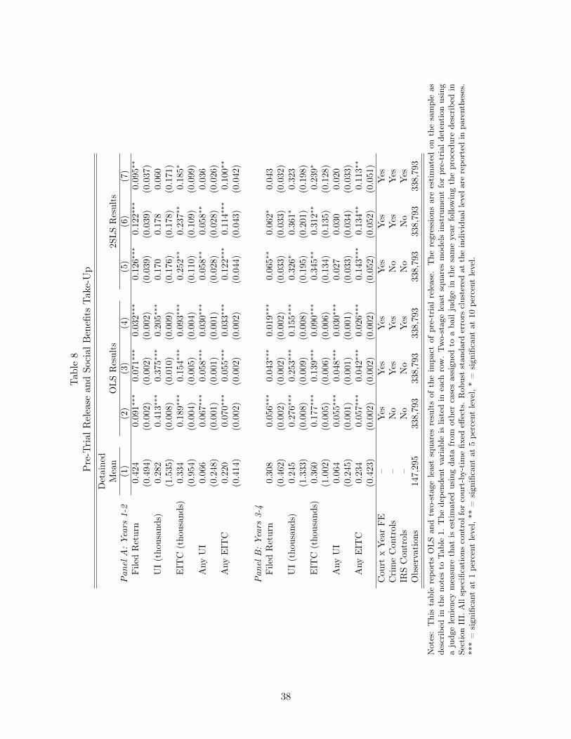
Tab

le8

Pre-Trial

Release

andSo

cial

Benefi

tsTake-Up

Detained

Mean

OLS

Results

2SLS

Results

Pan

elA

:Yea

rs1-

2(1)

(2)

(3)

(4)

(5)

(6)

(7)

FiledReturn

0.424

0.09

1∗∗∗

0.07

1∗∗∗

0.03

2∗∗∗

0.12

6∗∗∗

0.12

2∗∗∗

0.09

5∗∗

(0.494

)(0.002

)(0.002

)(0.002

)(0.039)

(0.039

)(0.037

)UI(tho

usan

ds)

0.28

20.41

3∗∗∗

0.37

5∗∗∗

0.20

5∗∗∗

0.17

00.17

80.06

0(1.535

)(0.008

)(0.010

)(0.009

)(0.176

)(0.178

)(0.171

)EIT

C(tho

usan

ds)

0.33

40.18

9∗∗∗

0.15

4∗∗∗

0.09

3∗∗∗

0.25

2∗∗

0.23

7∗∗

0.18

5∗

(0.954

)(0.004

)(0.005

)(0.004

)(0.110)

(0.109

)(0.099

)Any

UI

0.06

60.06

7∗∗∗

0.05

8∗∗∗

0.03

0∗∗∗

0.05

8∗∗

0.05

8∗∗

0.03

6(0.248

)(0.001

)(0.001

)(0.001

)(0.028)

(0.028

)(0.026

)Any

EIT

C0.22

00.07

0∗∗∗

0.05

5∗∗∗

0.03

3∗∗∗

0.12

2∗∗∗

0.11

4∗∗∗

0.10

0∗∗

(0.414

)(0.002

)(0.002

)(0.002

)(0.044)

(0.043

)(0.042

)

Pan

elB:Yea

rs3-

4FiledReturn

0.30

80.05

6∗∗∗

0.04

3∗∗∗

0.01

9∗∗∗

0.06

5∗∗

0.06

2∗0.04

3(0.462

)(0.002

)(0.002

)(0.002

)(0.033)

(0.033

)(0.032

)UI(tho

usan

ds)

0.24

50.27

6∗∗∗

0.25

3∗∗∗

0.15

5∗∗∗

0.32

6∗0.36

1∗0.32

3(1.333

)(0.008

)(0.009

)(0.008

)(0.195)

(0.201

)(0.198

)EIT

C(tho

usan

ds)

0.36

00.17

7∗∗∗

0.13

9∗∗∗

0.09

0∗∗∗

0.34

5∗∗

0.31

2∗∗

0.23

9∗

(1.002

)(0.005

)(0.006

)(0.006

)(0.134)

(0.135

)(0.128

)Any

UI

0.06

40.05

5∗∗∗

0.04

8∗∗∗

0.03

0∗∗∗

0.02

70.03

00.02

0(0.245

)(0.001

)(0.001

)(0.001

)(0.033

)(0.034

)(0.033

)Any

EIT

C0.23

40.05

7∗∗∗

0.04

2∗∗∗

0.02

6∗∗∗

0.14

3∗∗∗

0.13

4∗∗

0.11

3∗∗

(0.423

)(0.002

)(0.002

)(0.002

)(0.052)

(0.052

)(0.051

)Cou

rtxYearFE

–Yes

Yes

Yes

Yes

Yes

Yes

CrimeCon

trols

–No

Yes

Yes

No

Yes

Yes

IRSCon

trols

–No

No

Yes

No

No

Yes

Observation

s147,295

338,793

338,793

338,793

338,79

333

8,79

333

8,79

3

Notes:Thistablerepo

rtsOLSan

dtw

o-stag

eleastsqua

resresultsof

theim

pact

ofpre-trialrelease.

The

regression

sareestimated

onthesampleas

describe

din

theno

testo

Tab

le1.

The

depe

ndentvariab

leis

listedin

each

row.Two-stag

eleastsqua

resmod

elsinstrumentforpre-trialde

tentionusing

ajudg

elenien

cymeasure

that

isestimated

usingda

tafrom

othe

rcasesassign

edto

aba

iljudg

ein

thesameyear

follo

wingtheproced

urede

scribe

din

SectionIII.Allspecification

scontrolfor

court-by

-tim

efix

edeff

ects.Rob

uststan

dard

errors

clusteredat

theindividu

allevela

rerepo

rted

inpa

renthe

ses.

***=

sign

ificant

at1pe

rcentlevel,**

=sign

ificant

at5pe

rcentlevel,*=

sign

ificant

at10

percentlevel.

38

Table 9Results by Crime Characteristics

Crime Severity Crime TypeMisd. Felony Drug DUI Property Violent(1) (2) (3) (4) (5) (6)

Any Guilty Offense −0.190∗∗∗ −0.100 −0.108∗ 0.085 −0.143∗∗∗ −0.538(0.035) (0.068) (0.063) (0.121) (0.050) (0.382)[0.509] [0.543] [0.667] [0.528] [0.548] [0.291]

Guilty Plea −0.186∗∗∗ −0.012 −0.088 −0.028 −0.107∗∗ −0.203(0.032) (0.068) (0.061) (0.108) (0.049) (0.298)[0.214] [0.420] [0.349] [0.264] [0.411] [0.200]

Any Incarceration 0.017 −0.116∗ −0.128∗∗ 0.109 0.005 −0.274(0.019) (0.065) (0.055) (0.114) (0.043) (0.263)[0.112] [0.330] [0.255] [0.430] [0.223] [0.148]

Failure to Appear in Court 0.116∗∗∗ 0.210∗∗∗ 0.193∗∗ 0.095 0.141∗∗∗ 0.120(0.041) (0.049) (0.079) (0.102) (0.036) (0.246)[0.201] [0.101] [0.237] [0.182] [0.187] [0.082]

Rearrest Prior to Disposition 0.084∗∗∗ 0.064 0.012 0.045 0.038 0.385(0.029) (0.074) (0.065) (0.097) (0.055) (0.359)[0.192] [0.254] [0.271] [0.163] [0.251] [0.142]

Employed in 1-2 Years 0.038 0.033 0.132∗ −0.060 −0.002 0.475(0.050) (0.075) (0.080) (0.114) (0.075) (0.318)[0.481] [0.418] [0.424] [0.601] [0.397] [0.490]

Any Income in 1-2 Years 0.114∗∗ 0.074 0.116 −0.020 0.044 0.627∗

(0.052) (0.078) (0.083) (0.121) (0.078) (0.345)[0.509] [0.480] [0.458] [0.591] [0.485] [0.524]

Employed in 3-4 Years 0.091 0.117 0.119 −0.031 −0.111 0.877∗∗

(0.061) (0.091) (0.096) (0.228) (0.105) (0.378)[0.458] [0.414] [0.407] [0.568] [0.387] [0.469]

Any Income in 3-4 Years 0.058 0.122 0.028 −0.183 0.057 0.576∗

(0.063) (0.092) (0.097) (0.239) (0.105) (0.329)[0.492] [0.486] [0.461] [0.556] [0.477] [0.500]

Court x Year FE Yes Yes Yes Yes Yes YesCrime Controls Yes Yes Yes Yes Yes YesIRS Controls Yes Yes Yes Yes Yes YesObservations 228,056 197,974 117,666 20,786 73,057 34,514

Notes: This table reports two-stage least squares results of the impact of pre-trial release for selected case types.The regressions are estimated on the judge sample as described in the notes to Table 1. The dependent variable islisted in each row. Two-stage least squares models instrument for pre-trial detention using a judge leniency measurethat is estimated using data from other cases assigned to a bail judge in the same year following the proceduredescribed in Section III. All specifications control for court-by-time fixed effects. Robust standard errors clusteredat the individual level are reported in parentheses. *** = significant at 1 percent level, ** = significant at 5 percentlevel, * = significant at 10 percent level.

39

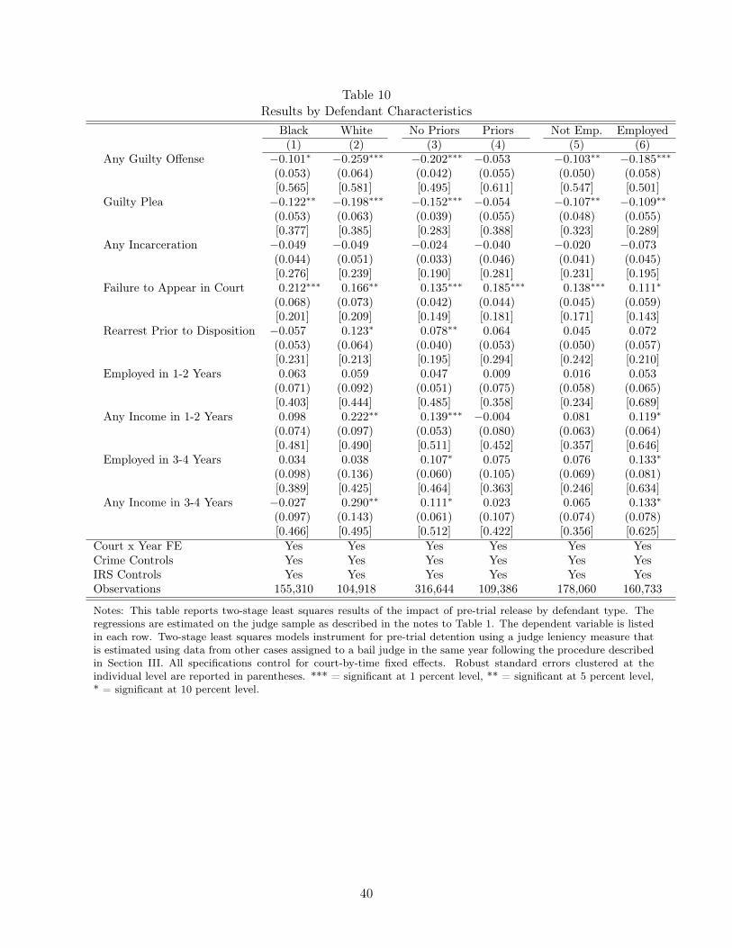
Table 10Results by Defendant Characteristics

Black White No Priors Priors Not Emp. Employed(1) (2) (3) (4) (5) (6)

Any Guilty Offense −0.101∗ −0.259∗∗∗ −0.202∗∗∗ −0.053 −0.103∗∗ −0.185∗∗∗

(0.053) (0.064) (0.042) (0.055) (0.050) (0.058)[0.565] [0.581] [0.495] [0.611] [0.547] [0.501]

Guilty Plea −0.122∗∗ −0.198∗∗∗ −0.152∗∗∗ −0.054 −0.107∗∗ −0.109∗∗

(0.053) (0.063) (0.039) (0.055) (0.048) (0.055)[0.377] [0.385] [0.283] [0.388] [0.323] [0.289]

Any Incarceration −0.049 −0.049 −0.024 −0.040 −0.020 −0.073(0.044) (0.051) (0.033) (0.046) (0.041) (0.045)[0.276] [0.239] [0.190] [0.281] [0.231] [0.195]

Failure to Appear in Court 0.212∗∗∗ 0.166∗∗ 0.135∗∗∗ 0.185∗∗∗ 0.138∗∗∗ 0.111∗

(0.068) (0.073) (0.042) (0.044) (0.045) (0.059)[0.201] [0.209] [0.149] [0.181] [0.171] [0.143]

Rearrest Prior to Disposition −0.057 0.123∗ 0.078∗∗ 0.064 0.045 0.072(0.053) (0.064) (0.040) (0.053) (0.050) (0.057)[0.231] [0.213] [0.195] [0.294] [0.242] [0.210]

Employed in 1-2 Years 0.063 0.059 0.047 0.009 0.016 0.053(0.071) (0.092) (0.051) (0.075) (0.058) (0.065)[0.403] [0.444] [0.485] [0.358] [0.234] [0.689]

Any Income in 1-2 Years 0.098 0.222∗∗ 0.139∗∗∗ −0.004 0.081 0.119∗

(0.074) (0.097) (0.053) (0.080) (0.063) (0.064)[0.481] [0.490] [0.511] [0.452] [0.357] [0.646]

Employed in 3-4 Years 0.034 0.038 0.107∗ 0.075 0.076 0.133∗

(0.098) (0.136) (0.060) (0.105) (0.069) (0.081)[0.389] [0.425] [0.464] [0.363] [0.246] [0.634]

Any Income in 3-4 Years −0.027 0.290∗∗ 0.111∗ 0.023 0.065 0.133∗

(0.097) (0.143) (0.061) (0.107) (0.074) (0.078)[0.466] [0.495] [0.512] [0.422] [0.356] [0.625]

Court x Year FE Yes Yes Yes Yes Yes YesCrime Controls Yes Yes Yes Yes Yes YesIRS Controls Yes Yes Yes Yes Yes YesObservations 155,310 104,918 316,644 109,386 178,060 160,733

Notes: This table reports two-stage least squares results of the impact of pre-trial release by defendant type. Theregressions are estimated on the judge sample as described in the notes to Table 1. The dependent variable is listedin each row. Two-stage least squares models instrument for pre-trial detention using a judge leniency measure thatis estimated using data from other cases assigned to a bail judge in the same year following the procedure describedin Section III. All specifications control for court-by-time fixed effects. Robust standard errors clustered at theindividual level are reported in parentheses. *** = significant at 1 percent level, ** = significant at 5 percent level,* = significant at 10 percent level.

40

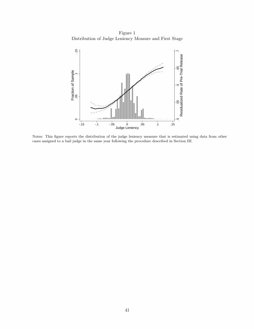
Figure 1Distribution of Judge Leniency Measure and First Stage

.5.5

5.6

.65

.7R

esid

ualiz

ed R

ate

of P

re-T

rial R

elea

se

0.0

5.1

.15

Frac

tion

of S

ampl

e

-.15 -.1 -.05 0 .05 .1 .15Judge Leniency

Notes: This figure reports the distribution of the judge leniency measure that is estimated using data from othercases assigned to a bail judge in the same year following the procedure described in Section III.

41

Appendix Table 1Descriptive Statistics by Bail Type

Initial Bail DecisionROR Non-Monetary Monetary

Panel A: Characteristics (1) (2) (3)Male 0.765 0.786 0.846White 0.422 0.434 0.382Black 0.555 0.556 0.604Age at Bail Decision 34.157 33.894 33.229Prior Offense in Past Year 0.145 0.277 0.281

Panel B: Charge CharacteristicsNumber of Offenses 1.887 2.047 3.735Felony Offense 0.134 0.423 0.633Misdemeanor Only 0.866 0.577 0.367Any Drug Offense 0.490 0.501 0.306Any DUI Offense 0.190 0.049 0.044Any Violent Offense 0.042 0.093 0.348Any Property Offense 0.165 0.281 0.268

Panel C: OutcomesAny Guilty Offense 0.516 0.569 0.493Guilty Plea 0.140 0.262 0.342Any Incarceration 0.132 0.184 0.267Failure to Appear in Court 0.251 0.263 0.099Absconded 0.013 0.007 0.002Days to Case Decision 261.294 232.109 229.731Rearrest Prior to Disposition 0.234 0.314 0.216Rearrest in 0-2 Years 0.373 0.479 0.414Rearrest in 3-4 Years 0.251 0.316 0.297Earnings (thousands) in 1-2 Years 8.015 5.871 6.460Employed in 1-2 Years 0.514 0.443 0.438Any Income in 1-2 Years 0.510 0.498 0.491Earnings (thousands) in 3-4 Years 8.657 6.380 7.049Employed in 3-4 Years 0.495 0.421 0.428Any Income in 3-4 Years 0.504 0.496 0.485

Panel D: Data QualityMissing Race 0.488 0.359 0.371

Observations 89,870 59,134 271,646

Notes: This table reports descriptive statistics by bail decision. The sample is described in the notes to Table 1. Seethe data appendix for additional details on the sample and variable construction.

42

Appendix Table 2Predictors of Pre-Trial Release

(1) (2) (3) (4)Residualized ROR Rate 0.020

(0.013)Residualized Non-Monetary Rate 0.146∗∗∗

(0.011)Residualized Monetary Rate −0.482∗∗∗

(0.019)Residualized Monetary Amount −0.002∗∗∗

(0.000)Observations 426,030 426,030 426,030 426,030

Notes: This table reports the pair-wise correlation between different judge leniency measures. The correlations arecalculated using the sample as described in the notes to Table 1. Judge leniency is estimated using data from othercases assigned to a bail judge the same year following the procedure described in Section III. *** = significant at 1percent level, ** = significant at 5 percent level, * = significant at 10 percent level.

43

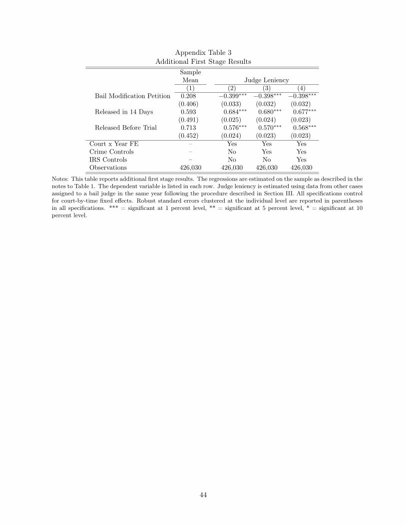
Appendix Table 3Additional First Stage Results

SampleMean Judge Leniency(1) (2) (3) (4)

Bail Modification Petition 0.208 −0.399∗∗∗ −0.398∗∗∗ −0.398∗∗∗

(0.406) (0.033) (0.032) (0.032)Released in 14 Days 0.593 0.684∗∗∗ 0.680∗∗∗ 0.677∗∗∗

(0.491) (0.025) (0.024) (0.023)Released Before Trial 0.713 0.576∗∗∗ 0.570∗∗∗ 0.568∗∗∗

(0.452) (0.024) (0.023) (0.023)Court x Year FE – Yes Yes YesCrime Controls – No Yes YesIRS Controls – No No YesObservations 426,030 426,030 426,030 426,030

Notes: This table reports additional first stage results. The regressions are estimated on the sample as described in thenotes to Table 1. The dependent variable is listed in each row. Judge leniency is estimated using data from other casesassigned to a bail judge in the same year following the procedure described in Section III. All specifications controlfor court-by-time fixed effects. Robust standard errors clustered at the individual level are reported in parenthesesin all specifications. *** = significant at 1 percent level, ** = significant at 5 percent level, * = significant at 10percent level.

44

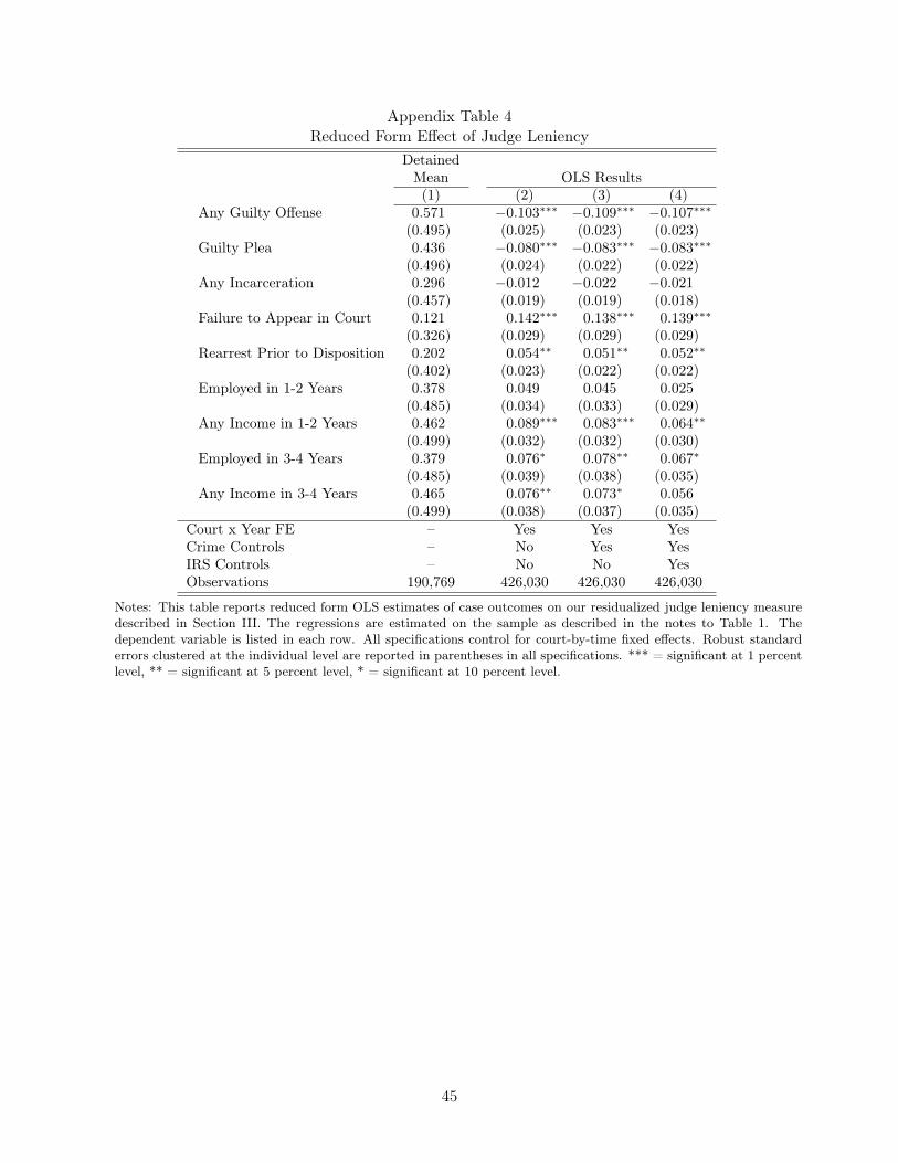
Appendix Table 4Reduced Form Effect of Judge Leniency

DetainedMean OLS Results(1) (2) (3) (4)

Any Guilty Offense 0.571 −0.103∗∗∗ −0.109∗∗∗ −0.107∗∗∗

(0.495) (0.025) (0.023) (0.023)Guilty Plea 0.436 −0.080∗∗∗ −0.083∗∗∗ −0.083∗∗∗

(0.496) (0.024) (0.022) (0.022)Any Incarceration 0.296 −0.012 −0.022 −0.021

(0.457) (0.019) (0.019) (0.018)Failure to Appear in Court 0.121 0.142∗∗∗ 0.138∗∗∗ 0.139∗∗∗

(0.326) (0.029) (0.029) (0.029)Rearrest Prior to Disposition 0.202 0.054∗∗ 0.051∗∗ 0.052∗∗

(0.402) (0.023) (0.022) (0.022)Employed in 1-2 Years 0.378 0.049 0.045 0.025

(0.485) (0.034) (0.033) (0.029)Any Income in 1-2 Years 0.462 0.089∗∗∗ 0.083∗∗∗ 0.064∗∗

(0.499) (0.032) (0.032) (0.030)Employed in 3-4 Years 0.379 0.076∗ 0.078∗∗ 0.067∗

(0.485) (0.039) (0.038) (0.035)Any Income in 3-4 Years 0.465 0.076∗∗ 0.073∗ 0.056

(0.499) (0.038) (0.037) (0.035)Court x Year FE – Yes Yes YesCrime Controls – No Yes YesIRS Controls – No No YesObservations 190,769 426,030 426,030 426,030

Notes: This table reports reduced form OLS estimates of case outcomes on our residualized judge leniency measuredescribed in Section III. The regressions are estimated on the sample as described in the notes to Table 1. Thedependent variable is listed in each row. All specifications control for court-by-time fixed effects. Robust standarderrors clustered at the individual level are reported in parentheses in all specifications. *** = significant at 1 percentlevel, ** = significant at 5 percent level, * = significant at 10 percent level.

45

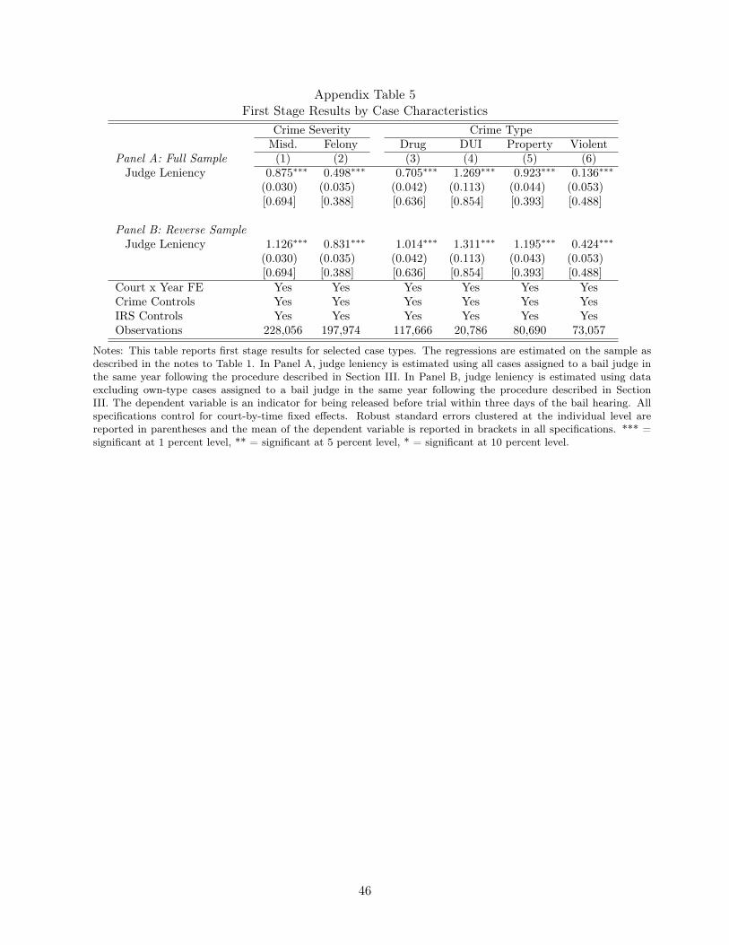
Appendix Table 5First Stage Results by Case Characteristics

Crime Severity Crime TypeMisd. Felony Drug DUI Property Violent

Panel A: Full Sample (1) (2) (3) (4) (5) (6)Judge Leniency 0.875∗∗∗ 0.498∗∗∗ 0.705∗∗∗ 1.269∗∗∗ 0.923∗∗∗ 0.136∗∗∗

(0.030) (0.035) (0.042) (0.113) (0.044) (0.053)[0.694] [0.388] [0.636] [0.854] [0.393] [0.488]

Panel B: Reverse SampleJudge Leniency 1.126∗∗∗ 0.831∗∗∗ 1.014∗∗∗ 1.311∗∗∗ 1.195∗∗∗ 0.424∗∗∗

(0.030) (0.035) (0.042) (0.113) (0.043) (0.053)[0.694] [0.388] [0.636] [0.854] [0.393] [0.488]

Court x Year FE Yes Yes Yes Yes Yes YesCrime Controls Yes Yes Yes Yes Yes YesIRS Controls Yes Yes Yes Yes Yes YesObservations 228,056 197,974 117,666 20,786 80,690 73,057

Notes: This table reports first stage results for selected case types. The regressions are estimated on the sample asdescribed in the notes to Table 1. In Panel A, judge leniency is estimated using all cases assigned to a bail judge inthe same year following the procedure described in Section III. In Panel B, judge leniency is estimated using dataexcluding own-type cases assigned to a bail judge in the same year following the procedure described in SectionIII. The dependent variable is an indicator for being released before trial within three days of the bail hearing. Allspecifications control for court-by-time fixed effects. Robust standard errors clustered at the individual level arereported in parentheses and the mean of the dependent variable is reported in brackets in all specifications. *** =significant at 1 percent level, ** = significant at 5 percent level, * = significant at 10 percent level.

46

Apppendix Table 6First Stage Results by Defendant Characteristics

Black White No Prior Prior Emp. Non-Emp.Panel A: Full Sample (1) (2) (3) (4) (5) (6)Judge Leniency 0.668∗∗∗ 0.601∗∗∗ 0.645∗∗∗ 0.810∗∗∗ 0.649∗∗∗ 0.715∗∗∗

(0.036) (0.039) (0.028) (0.041) (0.039) (0.035)[0.451] [0.491] [0.600] [0.415] [0.619] [0.517]

Panel B: Reverse SampleJudge Leniency 1.009∗∗∗ 0.969∗∗∗ 0.964∗∗∗ 1.050∗∗∗ 0.952∗∗∗ 1.005∗∗∗

(0.035) (0.039) (0.031) (0.041) (0.038) (0.035)[0.451] [0.491] [0.600] [0.415] [0.619] [0.517]

Court x Year FE Yes Yes Yes Yes Yes YesCrime Controls Yes Yes Yes Yes Yes YesIRS Controls Yes Yes Yes Yes Yes YesObservations 155,310 104,918 316,644 109,386 160,733 178,060

Notes: This table reports first stage results for selected defendant types. The regressions are estimated on the sampleas described in the notes to Table 1. In Panel A, judge leniency is estimated using all cases assigned to a bail judgein the same year following the procedure described in Section III. In Panel B, judge leniency is estimated using dataexcluding own-type cases assigned to a bail judge in the same year following the procedure described in SectionIII. The dependent variable is an indicator for being released before trial within three days of the bail hearing. Allspecifications control for court-by-time fixed effects. Robust standard errors clustered at the individual level arereported in parentheses and the mean of the dependent variable is reported in brackets in all specifications. *** =significant at 1 percent level, ** = significant at 5 percent level, * = significant at 10 percent level.

47

App

endixTab

le7

Add

itiona

lResults

Detained

Mean

OLS

Results

2SLS

Results

(1)

(2)

(3)

(4)

(5)

(6)

(7)

Num

berof

GuiltyOffe

nses

0.92

7−0.24

1∗∗∗

−0.07

8∗∗∗

−0.07

5∗∗∗

−0.18

2∗∗

−0.18

7∗∗∗

−0.186∗

∗∗

(1.745

)(0.004

)(0.004

)(0.004

)(0.074

)(0.069

)(0.069)

GuiltyPleato

Tim

eServed

0.20

2−0.14

0∗∗∗

−0.06

4∗∗∗

−0.06

2∗∗∗

−0.14

1∗∗∗

−0.13

1∗∗∗

−0.130∗

∗∗

(0.401

)(0.002

)(0.002

)(0.002

)(0.037

)(0.035

)(0.035)

Offe

nseCha

rged

Dow

n0.48

20.01

5∗∗∗

0.05

1∗∗∗

0.04

8∗∗∗

0.08

2∗∗

0.08

8∗∗

0.086∗

∗

(0.500

)(0.002

)(0.002

)(0.002

)(0.036

)(0.035

)(0.035)

Max

DaysIncarcerated

332.24

4−29

3.07

5∗∗∗

−15

6.55

7∗∗∗

−15

5.80

5∗∗∗

−14

4.04

9−14

6.11

2−14

4.745

(2,617.92

8)(4.197

)(4.227

)(4.554

)(210.643

)(211.005

)(211.974)

Cou

rtxYearFE

–Yes

Yes

Yes

Yes

Yes

Yes

CrimeCon

trols

–No

Yes

Yes

No

Yes

Yes

IRSCon

trols

–No

No

Yes

No

No

Yes

Observation

s190,769

426,030

426,030

426,030

426,03

042

6,03

042

6,03

0

Notes:Thistablerepo

rtsad

dition

alOLSan

dtw

o-stag

eleastsqua

resresultsof

theim

pact

ofpre-trialrelease.

The

regression

sareestimated

onthe

sampleas

describe

din

theno

testo

Tab

le1.

The

depe

ndentvariab

leis

listedin

each

row.

Two-stag

eleastsqua

resmod

elsinstrumentforpre-trial

detentionusingajudg

elenien

cymeasure

that

isestimated

usingda

tafrom

othe

rcasesassign

edto

aba

iljudg

ein

thesameyear

follo

wingtheproced

ure

describe

din

SectionIII.Allspecification

scontrolfor

court-by

-tim

efix

edeff

ects.Rob

uststan

dard

errors

clusteredat

theindividu

allevela

rerepo

rted

inpa

renthe

ses.

***=

sign

ificant

at1pe

rcentlevel,**

=sign

ificant

at5pe

rcentlevel,*=

sign

ificant

at10

percentlevel.

48

Appendix Table 8First Stage Results by Release Type

Judge LeniencySample No WithMean Conditions Conditions(1) (2) (3)

Released with No Conditions 0.203 0.938∗∗∗ −0.040∗∗∗

(0.402) (0.017) (0.014)Released with Conditions 0.349 −0.265∗∗∗ 0.728∗∗∗

(0.477) (0.026) (0.024)Court x Year FE – Yes YesCrime Controls – Yes YesIRS Controls – Yes YesObservations 426,030 426,030 426,030

Notes: This table reports additional first stage results for two types of pre-trial release: release ROR with no conditionsand release with conditions. The regressions are estimated on the sample as described in the notes to Table 1. Thedependent variable is listed in each row. Estimates in columns 2 and 3 are from the same OLS specification. Judgeleniency is estimated using data from other cases assigned to a bail judge in the same year following the proceduredescribed in Section III. All specifications control for court-by-time fixed effects. Robust standard errors clusteredat the individual level are reported in parentheses in all specifications. *** = significant at 1 percent level, ** =significant at 5 percent level, * = significant at 10 percent level.

49

Appendix Table 9Results by Release Type

OLS Results 2SLS ResultsDetained No With No WithMean Conditions Conditions Conditions Conditions(1) (2) (3) (4) (5)

Any Guilty Offense 0.571 −0.075∗∗∗ −0.042∗∗∗ −0.168∗∗∗ −0.154∗∗∗

(0.495) (0.002) (0.002) (0.036) (0.034)Guilty Plea 0.436 −0.137∗∗∗ −0.079∗∗∗ −0.129∗∗∗ −0.119∗∗∗

(0.496) (0.002) (0.002) (0.034) (0.032)Any Incarceration 0.296 −0.107∗∗∗ −0.096∗∗∗ −0.015 −0.032

(0.457) (0.002) (0.001) (0.028) (0.027)Failure to Appear in Court 0.121 0.060∗∗∗ −0.006∗∗∗ 0.178∗∗∗ 0.151∗∗∗

(0.326) (0.002) (0.001) (0.033) (0.031)Rearrest Prior to Disposition 0.202 0.058∗∗∗ 0.058∗∗∗ 0.091∗∗∗ 0.074∗∗

(0.402) (0.002) (0.002) (0.034) (0.033)Employed in 1-2 Years 0.378 0.053∗∗∗ 0.050∗∗∗ 0.042 0.037

(0.485) (0.003) (0.002) (0.046) (0.043)Any Income in 1-2 Years 0.462 0.036∗∗∗ 0.036∗∗∗ 0.094∗∗ 0.097∗∗

(0.499) (0.003) (0.002) (0.048) (0.045)Employed in 3-4 Years 0.379 0.041∗∗∗ 0.029∗∗∗ 0.085 0.102∗

(0.485) (0.003) (0.002) (0.055) (0.053)Any Income in 3-4 Years 0.465 0.032∗∗∗ 0.029∗∗∗ 0.045 0.087

(0.499) (0.003) (0.002) (0.056) (0.054)Court x Year FE – Yes Yes Yes YesCrime Controls – Yes Yes Yes YesIRS Controls – Yes Yes Yes YesObservations 190,769 426,030 426,030 426,030 426,030

Notes: This table reports OLS and two-stage least squares results of the impact of two types of pre-trial release:release ROR with no conditions and release with conditions. The regressions are estimated on the sample as describedin the notes to Table 1. The dependent variable is listed in each row. Estimates in columns 2 and 3 are from thesame OLS specification, and estimates in columns 4 and 5 are from the same two-stage least squares specification.All specifications control for court-by-time fixed effects. Robust standard errors clustered at the individual level arereported in parentheses. *** = significant at 1 percent level, ** = significant at 5 percent level, * = significant at 10percent level.

50

App

endixTab

le10

Rob

ustnessof

Two-StageLe

astSq

uaresResults

Judg

eLe

niency

Crime

Crime

Release

Non

-Mon

eySp

litSchedu

led

Severity

Typ

eEver

Bail

Sample

Judg

eJu

dgeFE

(1)

(2)

(3)

(4)

(5)

(6)

(7)

Any

GuiltyOffe

nse

−0.14

1∗∗∗

−0.17

3∗∗∗

−0.21

2∗∗∗

−0.07

6∗∗∗

−0.17

4∗∗∗

−0.14

7∗∗∗

−0.19

2∗∗∗

(0.027

)(0.027

)(0.039

)(0.021

)(0.039

)(0.036

)(0.034

)GuiltyPlea

−0.13

1∗∗∗

−0.13

4∗∗∗

−0.20

3∗∗∗

−0.04

5∗∗

−0.13

1∗∗∗

−0.12

9∗∗∗

−0.16

6∗∗∗

(0.026

)(0.026

)(0.038

)(0.020

)(0.038

)(0.035

)(0.032

)Any

Incarceration

0.01

2−0.04

3∗∗

−0.03

5−0.01

0−0.03

5−0.03

2−0.04

4(0.021

)(0.021

)(0.030

)(0.017

)(0.031

)(0.029

)(0.027

)Fa

ilure

toApp

earin

Cou

rt0.11

6∗∗∗

0.14

8∗∗∗

0.23

5∗∗∗

0.08

1∗∗∗

0.12

8∗∗∗

0.11

7∗∗∗

0.09

7∗∗∗

(0.026

)(0.023

)(0.049

)(0.018

)(0.036

)(0.036

)(0.037

)RearrestPrior

toDispo

sition

0.07

5∗∗∗

0.10

1∗∗∗

0.08

6∗∗

0.06

5∗∗∗

0.06

00.06

8∗0.06

2∗

(0.025

)(0.025

)(0.039

)(0.020

)(0.038

)(0.036

)(0.033

)Employed

in1-2Years

0.04

10.02

60.01

00.02

30.04

00.04

70.01

7(0.036

)(0.035

)(0.065

)(0.027

)(0.049

)(0.048

)(0.039

)Any

Incomein

1-2Years

0.07

0∗0.04

20.12

8∗−0.00

50.03

30.12

3∗∗

0.04

0(0.038

)(0.036

)(0.068

)(0.028

)(0.051

)(0.050

)(0.040

)Employed

in3-4Years

0.02

70.06

9∗0.09

20.07

3∗∗

0.09

10.09

10.08

0∗

(0.043

)(0.041

)(0.079

)(0.032

)(0.060

)(0.058

)(0.045

)Any

Incomein

3-4Years

0.05

00.02

00.16

2∗∗

0.03

00.07

40.09

50.02

9(0.044

)(0.041

)(0.081

)(0.032

)(0.061

)(0.059

)(0.046

)Cou

rtxYearFE

Yes

Yes

Yes

Yes

Yes

Yes

Yes

CrimeCon

trols

Yes

Yes

Yes

Yes

Yes

Yes

Yes

IRSCon

trols

Yes

Yes

Yes

Yes

Yes

Yes

Yes

Observation

s426,030

426,030

426,030

426,030

319,67

742

6,03

042

6,03

0

Notes:Thistablerepo

rtsrobu

stne

sschecks

ofou

rtw

o-stag

eleastsqua

resresults.

The

regression

sareestimated

onthesampleas

describe

din

theno

tes

toTab

le1.

The

depe

ndentvariab

leis

listedin

each

row.Colum

n1allowsjudg

elenien

cyto

vary

across

felonies

andmisde

meano

rs.Colum

n2allows

judg

elenien

cyto

vary

across

the5mutua

llyexclusivecrim

etype

s.Colum

n3uses

anindicatorforever

beingreleased

before

trialto

calculatejudg

elenien

cy.Colum

n4uses

anindicatorfortheassign

mentof

non-mon

etaryba

il.Colum

n5calculates

judg

elenien

cyusinga25

percentrand

omsubset

oftheda

taan

destimates

thetreatm

enteff

ects

intheop

posing

subset

ofda

ta.Colum

n6uses

thesche

duledba

iljudg

eto

calculatejudg

elenien

cy.Colum

n7uses

anexha

ustive

setof

judg

efix

edeff

ects

asinstruments.Allspecification

scontrolforcourt-by

-tim

efix

edeff

ects.Rob

uststan

dard

errors

clustered

attheindividu

allevelarerepo

rted

inpa

renthe

ses.

***=

sign

ificant

at1pe

rcentlevel,**

=sign

ificant

at5pe

rcentlevel,*=

sign

ificant

at10

percent

level.

51

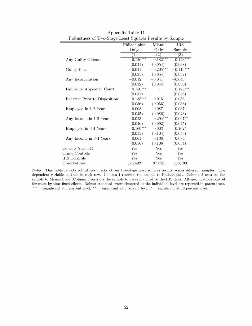
Appendix Table 11Robustness of Two-Stage Least Squares Results by Sample

Philadelphia Miami IRSOnly Only Sample(1) (2) (3)

Any Guilty Offense −0.126∗∗∗ −0.182∗∗∗ −0.143∗∗∗

(0.041) (0.054) (0.038)Guilty Plea −0.041 −0.205∗∗∗ −0.113∗∗∗

(0.035) (0.054) (0.037)Any Incarceration −0.012 −0.041 −0.043

(0.032) (0.044) (0.030)Failure to Appear in Court 0.150∗∗∗ – 0.125∗∗∗

(0.031) (0.036)Rearrest Prior to Disposition 0.135∗∗∗ 0.015 0.058

(0.036) (0.056) (0.038)Employed in 1-2 Years −0.003 0.087 0.037

(0.045) (0.086) (0.043)Any Income in 1-2 Years −0.023 0.294∗∗∗ 0.097∗∗

(0.046) (0.092) (0.045)Employed in 3-4 Years 0.160∗∗∗ 0.003 0.102∗

(0.055) (0.104) (0.053)Any Income in 3-4 Years 0.061 0.138 0.085

(0.056) (0.106) (0.054)Court x Year FE Yes Yes YesCrime Controls Yes Yes YesIRS Controls Yes Yes YesObservations 328,492 97,538 338,793

Notes: This table reports robustness checks of our two-stage least squares results across different samples. Thedependent variable is listed in each row. Column 1 restricts the sample to Philadelphia. Column 2 restricts thesample to Miami-Dade. Column 3 restricts the sample to cases matched to the IRS data. All specifications controlfor court-by-time fixed effects. Robust standard errors clustered at the individual level are reported in parentheses.*** = significant at 1 percent level, ** = significant at 5 percent level, * = significant at 10 percent level.

52

App

endixTab

le12

Effe

ctson

JointProba

bilitiesof

Con

victionan

dEmploy

ment

Detained

Mean

OLS

Results

2SLS

Results

Pan

elA

:Yea

rs1-

2(1)

(2)

(3)

(4)

(5)

(6)

(7)

Guiltyan

dEmployed

0.18

70.02

8∗∗∗

0.02

2∗∗∗

0.00

0−0.05

4∗−0.05

9∗−0.07

2∗∗

(0.390

)(0.001

)(0.002

)(0.002

)(0.033

)(0.032

)(0.031

)Guiltyan

dNot

Employed

0.33

3−0.09

5∗∗∗

−0.07

0∗∗∗

−0.04

5∗∗∗

−0.07

5∗∗

−0.07

5∗∗

−0.06

1∗

(0.471

)(0.002

)(0.002

)(0.002

)(0.036

)(0.035

)(0.034

)Not

Guiltyan

dEmployed

0.15

20.09

0∗∗∗

0.06

9∗∗∗

0.04

5∗∗∗

0.10

7∗∗∗

0.10

9∗∗∗

0.09

5∗∗∗

(0.359

)(0.001

)(0.002

)(0.002

)(0.032

)(0.031

)(0.031

)Not

Guiltyan

dNot

Employed

0.22

5−0.02

4∗∗∗

−0.02

2∗∗∗

−0.00

10.02

20.02

50.03

7(0.417

)(0.002

)(0.002

)(0.002

)(0.033

)(0.033

)(0.032

)

Pan

elB:Yea

rs3-

4Guiltyan

dEmployed

0.13

80.00

9∗∗∗

0.00

9∗∗∗

−0.00

5∗∗∗

−0.00

3−0.00

5−0.01

4(0.345

)(0.001

)(0.001

)(0.001

)(0.028

)(0.027

)(0.027

)Guiltyan

dNot

Employed

0.23

7−0.05

3∗∗∗

−0.03

6∗∗∗

−0.02

0∗∗∗

−0.03

9−0.03

9−0.02

9(0.425

)(0.001

)(0.002

)(0.001

)(0.031

)(0.031

)(0.030

)Not

Guiltyan

dEmployed

0.10

80.05

7∗∗∗

0.04

2∗∗∗

0.02

5∗∗∗

0.06

4∗∗

0.06

4∗∗

0.05

5∗∗

(0.310

)(0.001

)(0.001

)(0.001

)(0.027

)(0.027

)(0.026

)Not

Guiltyan

dNot

Employed

0.16

5−0.01

3∗∗∗

−0.01

4∗∗∗

−0.00

1−0.02

2−0.02

0−0.01

2(0.371

)(0.001

)(0.001

)(0.001

)(0.028

)(0.028

)(0.028

)Cou

rtxYearFE

–Yes

Yes

Yes

Yes

Yes

Yes

CrimeCon

trols

–No

Yes

Yes

No

Yes

Yes

IRSCon

trols

–No

No

Yes

No

No

Yes

Observation

s147,295

338,793

338,793

338,793

338,79

333

8,79

333

8,79

3

Notes:Thistablerepo

rtsad

dition

alOLSan

dtw

o-stag

eleastsqua

resresultsof

theim

pact

ofpre-trialr

elease

onthejointprob

ability

ofconv

iction

and

employment.

The

regression

sareestimated

onthesampleas

describe

din

theno

testo

Tab

le1.

The

depe

ndentvariab

leislistedin

each

row.Two-stag

eleastsqua

resmod

elsinstrumentforpre-trialde

tentionusingajudg

elenien

cymeasure

that

isestimated

usingda

tafrom

othe

rcasesassign

edto

aba

iljudg

ein

thesameyear

follo

wingtheproced

urede

scribe

din

SectionIII.Allspecification

scontrolfor

court-by

-tim

efix

edeff

ects.Rob

uststan

dard

errors

clusteredat

theindividu

allevelarerepo

rted

inpa

renthe

ses.

***=

sign

ificant

at1pe

rcentlevel,**

=sign

ificant

at5pe

rcentlevel,*=

sign

ificant

at10

percentlevel.

53

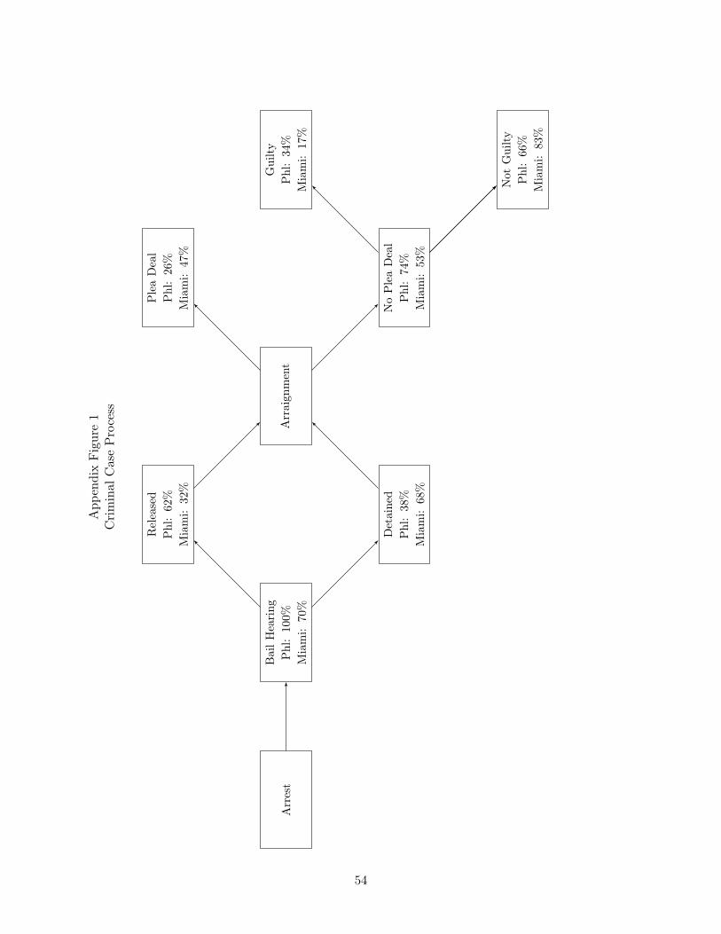
App

endixFigure1

Criminal

CaseProcess

Arrest

BailHearing

Phl:10

0%Miami:

70%

Detained

Phl:38%

Miami:

68%

Released

Phl:62%

Miami:

32%

Arraign

ment

PleaDeal

Phl:26

%Miami:

47%

NoPleaDeal

Phl:74

%Miami:

53%

Not

Guilty

Phl:66

%Miami:

83%

Guilty

Phl:34

%Miami:

17%

54

App

endixFigure2

BailG

uidelin

esin

Philadelphia

PHIL

ADEL

PHIA

BAI

L G

UID

ELIN

ES G

RID

L

OW

<--

----

----

----

----

----

----

----

----

----

----

----

-Cha

rge

Serio

usne

ss--

----

----

----

----

----

----

----

----

----

----

----

----

----

----

--->

HIG

H

1

2

3

4

5

6

7

8

9

10

HIGH <----------Risk Level--------> LOW

1

R

OR

1

R

OR

5

R

OR

9

R

OR

13

R

OR

17

R

OR

21

R

OR

25

$1,5

00-

$4,5

00

29

$2,2

00-

$6,7

00

33

$3,0

00-

$12,

000

37

2

R

OR

2

R

OR

6

R

OR

10

R

OR

14

R

OR

18

R

OSC

1

22

R

OSC

1

26

$3,0

00-

$6,7

00

30

$3,7

00-

$8,2

00

34

$3,7

00-

$12,

000

38

3

R

OR

3

R

OSC

1

7

R

OSC

1

11

R

OSC

1

15

R

OSC

2

19

R

OSC

2

23

R

OSC

2

27

$3,7

00-

$7,5

00

31

$4,5

00-

$9,7

00

35

$6,7

00-

$22,

500

39

4

R

OSC

1

4

R

OSC

1

8

R

OSC

1

12

R

OSC

2

16

R

OSC

2

20

R

OSC

2

24

$3,7

00-

$6,7

00

28

$4,5

00-

$7,5

00

32

$4,5

00-

$12,

000

36

$9,0

00-

$75,

000

40

Upd

ated

: Sep

tem

ber 1

2, 2

012

Notes:Thisfig

ureillustrates

theba

ilgu

idelines

inPhilade

lphia.

The

guidelines

classify

defend

ants

into

40po

ssible

catego

ries

andsugg

estfour

basic

type

sof

releaseop

tion

s.Cha

rgeseriou

snessrang

esfrom

oneto

10,with10

themostseriou

s.Risklevelrang

esfrom

oneto

four,withfour

thehigh

est

risk,an

dis

basedon

therisk

ofade

fend

antfailing

toap

pear

incourtan

dcommitting

new

offen

ses.

ROR

isreleaseon

recogn

izan

ce.ROSC

isrelease

onspecialc

ondition

s.

55

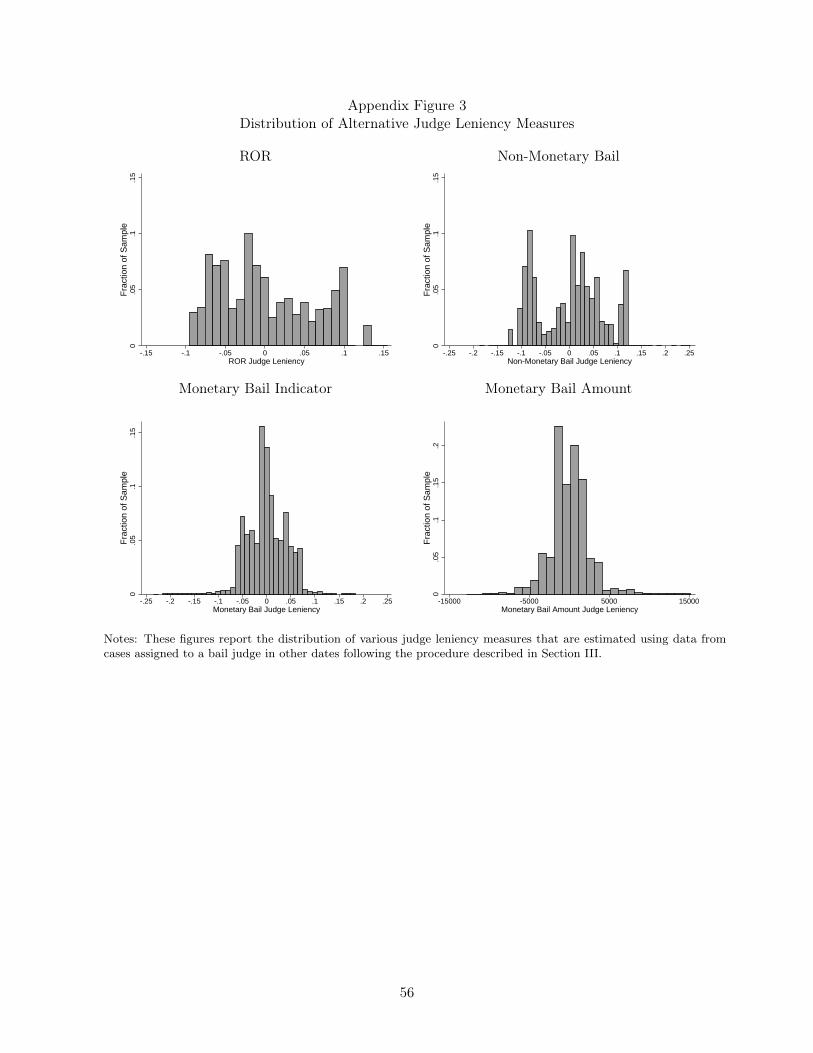
Appendix Figure 3Distribution of Alternative Judge Leniency Measures

ROR Non-Monetary Bail

0.0

5.1

.15

Fra

ctio

n of

Sam

ple

-.15 -.1 -.05 0 .05 .1 .15ROR Judge Leniency

0.0

5.1

.15

Fra

ctio

n of

Sam

ple

-.25 -.2 -.15 -.1 -.05 0 .05 .1 .15 .2 .25Non-Monetary Bail Judge Leniency

Monetary Bail Indicator Monetary Bail Amount

0.0

5.1

.15

Fra

ctio

n of

Sam

ple

-.25 -.2 -.15 -.1 -.05 0 .05 .1 .15 .2 .25Monetary Bail Judge Leniency

0.0

5.1

.15

.2F

ract

ion

of S

ampl

e

-15000 -5000 5000 15000Monetary Bail Amount Judge Leniency

Notes: These figures report the distribution of various judge leniency measures that are estimated using data fromcases assigned to a bail judge in other dates following the procedure described in Section III.

56

Appendix Figure 4Judge Leniency by Defendant and Case Characteristics

β = 0.189 (0.121)

-.3-.2

-.10

.1.2

.3N

on-F

elon

y

-.3 -.2 -.1 0 .1 .2 .3Felony

β = 0.181 (0.092)

-.05

-.025

0.0

25.0

5N

on-D

UI

-.05 -.025 0 .025 .05DUI

β = 0.152 (0.059)

-.25

-.15

-.05

.05

.15

.25

Non

-Dru

g

-.4 -.3 -.2 -.1 0 .1 .2 .3 .4Drug

β = 0.212 (0.029)

-.25

-.15

-.05

.05

.15

.25

Non

-Pro

perty

-.4 -.3 -.2 -.1 0 .1 .2 .3 .4Property

β = 0.032 (0.050)

-.3-.2

-.10

.1.2

.3N

on-V

iole

nt

-.4 -.3 -.2 -.1 0 .1 .2 .3 .4Violent

β = 0.388 (0.047)

-.25

-.15

-.05

.05

.15

.25

Blac

k

-.25 -.15 -.05 .05 .15 .25White

β = 0.259 (0.042)

-.25

-.15

-.05

.05

.15

.25

No

Prio

r Offe

nse

-.25 -.15 -.05 .05 .15 .25Prior Offense

b = 0.401 (0.077)

-.25

-.15

-.05

.05

.15

.25

Not

Em

ploy

ed

-.25 -.15 -.05 .05 .15 .25Employed

Notes: These figures show the correlation between our residualized measure of judge leniency for different groupsof defendants. DUI cases are only available in Philadelphia. We take the average leniency for each group over allavailable years of data. The solid line shows the best linear fit estimated using OLS relating each judge leniencymeasure.

57