the effects of human resource management practices...
TRANSCRIPT
The Effects of Human Resource Management Practices on Productivity: A Study of Steel Finishing Lines
By CASEY ICHNIOWSKI, KATHRYN SHAW, AND GIOVANNA PRENNUSHI*
We investigate the productivity effects of innovative employment practices using data from a sample of 36 homogeneous steel production lines owned by 17 com- panies. The productivity regressions demonstrate that lines using a set of inno- vative work practices, which include incentive pay, teams, flexible job assignments, employment security, and training, achieve substantially higher lev- els of productivity than do lines with the more traditional approach, which in- cludes narrow job definitions, strict work rules, and hourly pay with close supervision. Our results are consistent with recent theoretical models which stress the importance of complementarities among work practices. (JEL J24, J5, L20, M11)
This study presents new empirical evidence on the productivity effects of alternative em- ployment practices using data that we have as- sembled on steel finishing processes. The unique data set makes this study's estimates of productivity differentials due to employment practices particularly convincing for several reasons. First, the data set is restricted to ob- servations on one very specific type of manu- facturing production process. This narrow focus eliminates many sources of heterogeneity that confound productivity comparisons in
more aggregate data and in more heterogeneous samples. Second, we develop a detailed model of this particular production process based on personal visits to each work site. We estimate the productivity model using precise measures of productivity, capital equipment, employment practices, and other line-specific determinants of productivity that we collected from each work site. Third, we obtain longitudinal data on each production line to estimate fixed-effects models that investigate changes in productivity within production lines due to changes in their employment practices. The primary limitation of the study is, of course, that it reflects work practices and performance outcomes in only one industry.
We find consistent support for the conclu- sion that groups or clusters of complementary human resource management (HRM) prac- tices have large effects on productivity, while changes in individual work practices have lit- tle or no effect on productivity. In Section I we describe the unique sample and data as- sembled for this study. Section II identifies studies in the incentive contract literature which stress the importance of complementar- ities among employment practices, while Sec- tion III develops measures of the production lines' HRM practices. In Sections IV-VI we present alternative econometric specifications of the productivity model and the empirical estimates. Section VII offers a conclusion.
* Ichniowski: Graduate School of Business, 713 Uris Hall, Columbia University, New York, NY 10027; Shaw: Graduate School of Industrial Administration, Camegie Mellon University, Pittsburgh, PA 15213; Prennushi: The World Bank, 1818 H St., NW, Washington, DC 20433. Principal coinvestigators Ichniowski and Shaw acknowl- edge the valued support of the Alfred P. Sloan Founda- tion's Steel Industry Center of Carnegie Mellon University and the Columbia University Center for Japanese Econ- omy and Business. We also gratefully acknowledg6 help- ful comments from Richard Cyert, Robert Gibbons, Zvi Griliches, Daniel Hamermesh, James Heckman, Bengt Holmstrom, Paul Milgrom, and John Roberts. Valuable suggestions also were made by participants in the Amer- ican Economic Association meetings and in seminars at Cornell University, the Massachusetts Institute of Tech- nology, Harvard University, the University of Michigan, the University of Maryland, Columbia University, Ohio State University, Carnegie Mellon University, the Na- tional Bureau of Economic Research, the Bureau of Labor Statistics, and the Federal Reserve Board.
291
This content downloaded from 195.113.56.251 on Wed, 23 Sep 2015 20:05:07 UTCAll use subject to JSTOR Terms and Conditions
292 THE AMERICAN ECONOMIC REVIEW JUNE 1997
I. Sample and Data
A. Sample Design
Heterogeneity in production processes and outputs often limits the persuasiveness of em- pirical studies that make firm-level or plant- level productivity comparisons. Therefore, in designing our model of worker productivity, we sought to minimize heterogeneity by col- lecting a unique data set on a sample of steel- making operations. Observations in the sample are not of steel companies, divisions of steel companies, or even steel mills. Rather, the sample consists of observations on one very specific type of steel finishing process.
Of the approximately 60 finishing lines of this type in the United States, we personally visited 45 lines owned by 21 companies at lo- cations ranging from New York to Alabama to California. We conducted field interviews for one to three days at each site, collecting information on HRM practices, the perfor- mance of the finishing lines, the capital equip- ment used in the production processes, other inputs into the production process, and wage data. Four of the 45 lines could not provide performance data because they had been op- erating for only a few months. Of the remain- ing 41 lines, 36 lines provided comparable monthly productivity data.
This study's econometric analysis uses a panel data set of up to 2,190 monthly obser- vations on the productivity of these 36 steel finishing lines owned by 17 different steel companies. The sample includes multiple lines for major steel producers as well as lines for smaller companies that operate only one or two lines. The sample contains unionized lines as well as nonunion lines. According to com- pany and industry sources, the sample includes high and low performers and a wide range of HRM environments.
B. The Production Process and the Dependent Productivity Variable
To understand how to model the production process in these finishing lines and how to measure the lines' performance, we toured each line with an experienced engineer, area
operations manager, or superintendent. The basic production process is very similar in all lines. Steel input on each line is a roll (or coil) of flat-rolled steel weighing about 12 tons. The coil is loaded at the beginning of the line where the steel strip is welded to the end of the previous coil on the line. The coil then is unrolled so that a long, continuous sheet of steel threads its way through the machinery that treats the steel. After the finishing treat- ment, the steel strip is then re-coiled and cut at the exit end of the process. The line can operate continuously around the clock as coils are welded to one another.
The productivity model for this production process is best understood within the context of an "engineering production function." The tonnage that comes off the line per month (Q) is a function of the tonnage loaded onto the line-and therefore is a function of the width (w) and thickness or gauge (g) of the steel strip-times the speed of the line (s), and the hours it is running (h). If hS represents the maximum hours the line is scheduled to run, then the potential steel output on line i in month t is arithmetically determined by the four key technical parameters (w, g, s, and hs), and this can be expressed:
(1) Potential Qit = (wit,git,sit,W)
where the quantity in parentheses in equation (1 ) is the volume of steel through line i in month t, and w is an estimate of the density of steel.
Since the production parameters in equa- tion ( 1 ) are determined by the technical specifications of the line's equipment and the specifications of the input coil's width and gauge, a line's production in any month depends only on the number of hours the line actually runs:
(2) Actual Qit = ( wit * git * Sit * h sit
x (1-dit),
where dit is delays-the fraction of total scheduled hours that are lost because of un- scheduled line stops. Once the technological parameters and product mix are specified,
This content downloaded from 195.113.56.251 on Wed, 23 Sep 2015 20:05:07 UTCAll use subject to JSTOR Terms and Conditions
VOL. 87 NO. 3 ICHNIOWSKI ET AL: EFFECTS OF HR MANAGEMENT PRACTICES 293
production depends solely on delays. Produc- tivity improves by increasing uptime, (1 - dit).
Production-line uptime is our primary mea- sure of productivity, because uptime directly determines steel output and because uptime figures are especially comparable across com- panies. Uptime, Ui, = 1 - di,, is the percent of scheduled operating time that the line actually runs. In the sample of 2,190 "line-month" ob- servations used in the empirical analysis, up- time has a mean value of 0.919, a standard deviation of 0.044, and a range of 0.398 to 0.996. In addition to this output measure, we will provide results for the quality of output, as measured by the percent of tons produced that meet specific quality standards for the in- dustry. We focus primarily, however, on productivity.
C. Control Variables in the Productivity Equation
This study's focus on one specific pro- duction process eliminates many sources of heterogeneity in productivity, but these pro- duction lines are not identical. To provide a thorough set of controls for other sources of productivity variation, we personally in- spected each production line in the sample and discussed with engineering experts from the lines any technical features that affect uptime. Based on these discussions, we were able to identify and collect a comprehensive set of data on technological features of the lines that affect their productivity.
The uptime productivity equations include up to 25 controls for detailed features of the line that affect uptime. These are controls for capital vintage (the year the line was built and its square); "learning curve" effects (time since start-up of the line and its square, a dummy for the first year of operations, and a monthly time counter for the start-up period); technical line specifications (line width, line speed, and their squares); specific line ma- chinery that reduces or increases the likelihood of unscheduled downtime (a dummy for the degree of computerization on the line and nine dummies for specific design features of equip- ment); periods of unusually high downtime (variables for quarters when new equipment is
added to the line); the quality of steel input (a ranking of steel quality from potential U.S. suppliers); and the extent of scheduled down- time for maintenance activities (the number of annual eight-hour maintenance shifts). Ac- cording to our interviews and site inspections, unscheduled downtime should be higher in older lines, faster and wider lines, start-up pe- riods, lines with fewer computerized controls, periods when new equipment is installed, lines that perform less preventive maintenance, and lines with lower quality steel input.
D. Data on HRM Policies
We gathered human resource management data by conducting standardized interviews with HR managers, labor relations managers, operations managers of the finishing lines, su- perintendents, line workers, and union repre- sentatives in organized lines. We collected supporting information from personnel files, personnel manuals, collective bargaining agreements, and other primary source docu- ments. We used this information from the in- terviews and supporting documents to answer survey-type questions about the HRM prac- tices and then to construct a detailed set of HRM dummy variables.
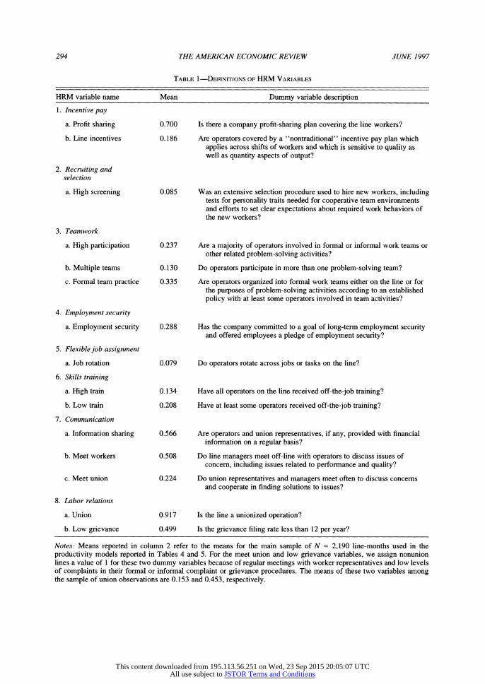
Table 1 provides the definitions of a subset of representative HRM variables and their mean values for the panel data set. These vari- ables measure work practices in all major areas of personnel management, including compen- sation, recruiting and selection, team-based work organization, employment security, flex- ible job assignment, skills training, and com- munication procedures. We also include two traditional labor relations indicators: the union status of the line and a grievance rate variable.
II. Complementarities Among Work Practices
Several empirical studies have examined the effects on a firm's productivity of individual work practices such as those listed in Table 1, including profit sharing (Douglas L. Kruse, 1993), training (Ann Bartel, 1995), or infor- mation sharing (Morris Kleiner and Marvin Bouillon, 1988). However, recent incentive contract theories argue that complementarities
This content downloaded from 195.113.56.251 on Wed, 23 Sep 2015 20:05:07 UTCAll use subject to JSTOR Terms and Conditions
294 THE AMERICAN ECONOMIC REVIEW JUNE 1997
TABLE 1-DEFINITIONS OF HRM VARIABLES
HRM variable name Mean Dummy variable description
1. Incentive pay
a. Profit sharing 0.700 Is there a company profit-sharing plan covering the line workers?
b. Line incentives 0.186 Are operators covered by a "nontraditional" incentive pay plan which applies across shifts of workers and which is sensitive to quality as well as quantity aspects of output?
2. Recruiting and selection
a. High screening 0.085 Was an extensive selection procedure used to hire new workers, including tests for personality traits needed for cooperative team environments and efforts to set clear expectations about required work behaviors of the new workers?
3. Teamwork
a. High participation 0.237 Are a majority of operators involved in formal or informal work teams or other related problem-solving activities?
b. Multiple teams 0.130 Do operators participate in more than one problem-solving team?
c. Formal team practice 0.335 Are operators organized into formal work teams either on the line or for the purposes of problem-solving activities according to an established policy with at least some operators involved in team activities?
4. Employment security
a. Employment security 0.288 Has the company committed to a goal of long-term employment security and offered employees a pledge of employment security?
5. Flexible job assignment
a. Job rotation 0.079 Do operators rotate across jobs or tasks on the line?
6. Skills training
a. High train 0.134 Have all operators on the line received off-the-job training?
b. Low train 0.208 Have at least some operators received off-the-job training?
7. Communication
a. Information sharing 0.566 Are operators and union representatives, if any, provided with financial information on a regular basis?
b. Meet workers 0.508 Do line managers meet off-line with operators to discuss issues of concern, including issues related to performance and quality?
c. Meet union 0.224 Do union representatives and managers meet often to discuss concerns and cooperate in finding solutions to issues?
8. Labor relations
a. Union 0.917 Is the line a unionized operation?
b. Low grievance 0.499 Is the grievance filing rate less than 12 per year?
Notes: Means reported in column 2 refer to the means for the main sample of N = 2,190 line-months used in the productivity models reported in Tables 4 and 5. For the meet union and low grievance variables, we assign nonunion lines a value of 1 for these two dummy variables because of regular meetings with worker representatives and low levels of complaints in their formal or informal complaint or grievance procedures. The means of these two variables among the sample of union observations are 0.153 and 0.453, respectively.
This content downloaded from 195.113.56.251 on Wed, 23 Sep 2015 20:05:07 UTCAll use subject to JSTOR Terms and Conditions
VOL 87 NO. 3 ICHNIOWSKI ET AL: EFFECTS OF HR MANAGEMENT PRACTICES 295
often exist among a firm's employment prac- tices. For example, one employment practice, such as the use of problem-solving teams, may be more effective in stimulating worker pro- ductivity when it is adopted in concert with other work practices that give workers the in- centive and the ability to perform well in teams-practices such as incentive pay, training, the flexible assignment of workers, or employment security. These theories argue that is important to analyze a firm's work pol- icies "not in isolation, but as part of a coherent incentive system" (Bengt Holmstrom and Paul Milgrom, 1994 p. 990; see also Milgrom and John Roberts, 1990, 1995; Eugene Kandel and Edward Lazear, 1992; George Baker et al., 1994).
According to these theories, interaction ef- fects among HRM policies are important de- terminants of productivity. Firms realize the largest gains in productivity by adopting clus- ters of complementary practices, and benefit little from making "marginal" changes in any one HRM practice. These theories also iden- tify complementarities among specific prac- tices which span seven different HRM policy areas: incentive compensation plans, extensive recruiting and selection, work teams, employ- ment security, flexible job assignment, skills training, and labor-management communica- tion.' Taken as a whole, these theories also predict that adopting this entire complement of practices across all seven HRM policy
areas will produce the highest levels of productivity.2
If firms adopt work practices in a comple- mentary fashion, then empirical tests should consider the impacts of groups of practices rather than simply the effects of individual practices. The primary hypothesis investigated in the empirical work is: do groups of inno- vative HRM practices increase productivity? The productivity effects of groups of innova- tive work practices also will be compared to the effects of differences in individual work practices.
III. HRM Systems
The argument that complementarities exist among HRM practices is consistent with the evidence that HRM policy variables are highly correlated with each other in our steel sample. Out of 78 possible bivariate correlations among the 13 HRM variables listed in Table 1, 71 are positive and 48 are positive and significant.3
Patterns in these correlations are consistent with the predictions of several authors. For ex- ample, Kandel and Lazear (1992) show how careful employee recruiting and team meetings can make group incentive pay more effective. In our data, line-specific incentive pay plans (line incentives in line lb of Table 1) are
' As examples, Kandel and Lazear (1992) show that teamwork and careful employee selection will make group-based incentive pay more effective by reducing free-rider problems. Baker et al. (1994) show that incentive pay plans based on objective performance mea- sures can increase the effectiveness of policies,such as work teams, which require subjective evaluations of em- ployees. Holmstrom and Milgrom (1994) model the complementarities that arise when workers perform multiple tasks and no one practice induces optimal effort on all tasks. Milgrom and Roberts (1995) argue that productivity-improvement teams are more effective when a firm adopts a set of complementary practices including employment security, flexible job assignments, skills training, and communication procedures. For further dis- cussion of the predictions of these theories, see Ichniowski et al. (1995 pp. 2-7).
2 The overlap among the policies considered in the the- ories discussed in footnote 1 implies that the most pro- ductive HRM system will have innovative work practices in all seven HRM areas. For example, Baker et al. (1994) consider complementarities between objective incentive pay and subjective performance appraisals or problem- solving teams. But Kandel and Lazear (1992) argue that careful screening, indoctrination, and teamwork make ob- jective incentives more effective, so these policies should be complements with policies like work teams, which re- quire subjective appraisals of employees. Milgrom and Roberts ( 1995) also consider work teams, but indicate that this policy will be more effective in combination with job security, job flexibility, training, and communication.
' To construct the sample for calculating these corre- lations, we allow one observation for each distinct com- bination of HRM policies experienced by a line. The 36 production lines experienced a total of 54 different com- binations of the HRM practices listed in Table 1, and these 54 observations comprise the sample for calculating cor- relations among the HRM practices.
This content downloaded from 195.113.56.251 on Wed, 23 Sep 2015 20:05:07 UTCAll use subject to JSTOR Terms and Conditions
296 THE AMERICAN ECONOMIC REVIEW JUNE 1997
positively correlated with extensive recruiting (high screening, line 2a), with team-based work structures (formal team practice, line 3c and multiple teams, line 3b), and with labor- management meetings (meet workers, line 7b and meet union, line 7c). Baker et al. (1994) argue that incentive pay based on objective measures will be complementary to incentive pay based on subjective evaluations of em- ployees. The data here show that the line in- centives variable also is positively correlated with "subjective" incentive pay plans such as "pay-for-knowledge" policies, and with the level of worker involvement in teams (high participation, line 3a). Finally, Milgrom and Roberts (1995) argue that problem-solving teams will be more effective when firms also provide employment security, job flexibility, training, and communication procedures. In our sample, work team variables, the employ- ment security variable (line 4a), the high screening variable, various measures of labor- management communication (information sharing, line 7a; meet workers; meet union), and job flexibility (job rotation, line 5a) are highly correlated.4
This high degree of intercorrelation among HRM practices indicates that empirical mod- els that estimate the impact of any one HRM practice on productivity will yield biased co- efficients due to the omission of other HRM practices with which the one included prac- tice is correlated. One possible solution to this omitted variable problem would be to enter the entire set of potentially important HRM variables into the productivity equations. This approach, however, is confounded by the se- vere collinearity among the HRM practices, making any one coefficient uninterpretable, and would not directly test whether combi- nations of HRM practices are the critical de- terminants of productivity.5 To examine the importance of sets of highly correlated, and
presumably complementary, HRM practices, one must examine the effects of interactions among the practices. There are an insufficient number of degrees of freedom to test a full set of interaction terms among all available HRM practice variables. And, an expansive set of interaction terms still would be con- founded by collinearity among practices, so we seek to identify common clusters of practices.
A. Identifying Systems of HRM Practices
To summarize the overall HRM environ- ments of the work sites in our sample, we iden- tify the most common combinations of HRM practices in these production lines. Specifically, we examine an extensive set of variables that describe the seven HRM policy areas consid- ered in the theories discussed in Section II: sub- jective and objective incentive compensation plans, extensive recruiting and selection, team- work, employment security, job flexibility, training, and labor-management communica- tion.6 Combinations of practices that exist in our sample are referred to as "HRM systems."
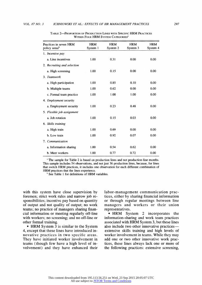
Table 2 reports four distinctive combinations of HRM practices identified by inspection of the distributions of the HRM variables. These four HRM systems map out a hierarchy from most "traditional" to most "innovative."
* HRM System 4 is the traditional system. It contains no innovative practices. Facilities
4 For the full set of correlations, see Ichniowski et al. (1995 pp. 13-15).
' Examining collinearity diagnostics (David A. Belsley et al., 1980) for our productivity model that includes all 15 HRM variables listed in Table 1 reveals a clear case of what Belsley et al. term "competing collinearity."
6 To provide as rich a description as possible of the overall HRM environment, we use more variables than the 15 HRM practices in Table 1. We use from one to six specific practices describing each of the seven HRM pol- icy areas. These other variables are dummies for inter- mediate levels of recruiting and screening activities; training in team problem-solving techniques and in statis- tical process control methods; the presence of informal work teams and local union support for team activities; employee participation in developing standard work prac- tices; multiattribute gainsharing incentive plans; "pay-for- knowledge" salary plans; and combined operator job classifications and combined maintenance worker job classifications. In all, 26 HRM policy variables are used to classify the lines' HRM environments. Because we are classifying lines according to their work practices, this set of 26 variables does not include the union status or the grievance rate variables listed in Table 1.
This content downloaded from 195.113.56.251 on Wed, 23 Sep 2015 20:05:07 UTCAll use subject to JSTOR Terms and Conditions
VOL 87 NO. 3 ICHNIOWSKI ET AL: EFFECTS OF HR MANAGEMENT PRACTICES 297
TABLE 2-PROPORTION OF PRODUCTION LINES WITH SPECIFIC HRM PRACTICES
WITHIN FOUR HRM SYSTEM CATEGORIESa
Practices in seven HRM HRM HRM HRM HRM policy areasb System 1 System 2 System 3 System 4
1. Incentive pay
a. Line incentives 1.00 0.31 0.00 0.00
2. Recruiting and selection
a. High screening 1.00 0.15 0.00 0.00
3. Teamwork
a. High participation 1.00 0.85 0.10 0.00
b. Multiple teams 1.00 0.62 0.00 0.00
c. Formal team practice 1.00 1.00 1.00 0.00
4. Employment security
a. Employment security 1.00 0.23 0.48 0.00
5. Flexible job assignment
a. Job rotation 1.00 0.15 0.03 0.00
6. Skills training
a. High train 1.00 0.69 0.00 0.00
b. Low train 1.00 0.92 0.07 0.00
7. Communication
a. Information sharing 1.00 0.54 0.62 0.00
b. Meet workers 1.00 0.77 0.72 0.00
a The sample for Table 2 is based on production lines and not production-line months. This sample includes 54 observations, and not just 36 production lines, because, for lines that switch HRM practices, it includes one observation for each different combination of HRM practices that the lines experience.
b See Table 1 for definitions of HRM variables.
with this system have close supervision by foremen; strict work rules and narrow job re- sponsibilities; incentive pay based on quantity of output and not quality of output; no work teams; no practice of managers sharing finan- cial information or meeting regularly off-line with workers; no screening; and no off-line or other formal training.
* HRM System 3 is similar to the System 4, except that these lines have introduced in- novative practices in two specific areas. They have initiated worker involvement in teams (though few have a high level of in- volvement) and they have enhanced their
labor-management communication prac- tices, either by sharing financial information or through regular meetings between line managers and workers or their union representatives.
* HRM System 2 incorporates the information-sharing and work team practices associated with HRM System 3, but these lines also include two other innovative practices- extensive skills training and high levels of worker involvement in teams. While they may add one or two other innovative work prac- tices, these lines always lack one or more of the following practices: extensive screening,
This content downloaded from 195.113.56.251 on Wed, 23 Sep 2015 20:05:07 UTCAll use subject to JSTOR Terms and Conditions
298 THE AMERICAN ECONOMIC REVIEW JUNE 1997
job rotation or reduced job classifications, multiattribute incentive pay, or employment security.7
* HRM System 1 incorporates innovative HRM practices in all HRM policy areas. Lines with this system have a multiattribute incentive pay plan or a "pay-for-knowledge" incentive pay system; extensive screening of new workers, often lasting over one year; off-line training in technical skills and team problem solving; high levels of employee involvement in multiple problem-solving teams; job duties covering a wide range of tasks with workers often rotating across jobs; regular information sharing between workers and management; and an implicit em- ployment security pledge.
In addition to identifying the common HRM systems by inspecting the distribution of HRM dummy variables in the sample, we also use three statistical procedures to identify common HRM systems. The alternative statistical clas- sification procedures produce system classifi- cations that overlap very closely with those system classifications described above, sug- gesting that the classification of lines' HRM environments is robust with respect to differ- ent classification procedures.8 We will use the "systems" reported in Table 2 as the basic HRM measures in the productivity regres-
sions, but also present regression results in- troducing HRM systems from one of the alternative classification procedures to illus- trate the similarity of the results when HRM systems are measured with a different procedure.
B. The Distribution and Average Productivities of HRM Systems
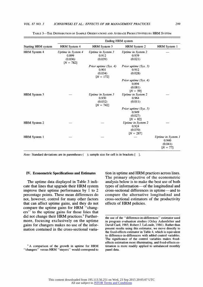
Table 3 shows the distribution of the data and productivity means for the alternative HRM systems. While most lines do not change their HRM systems during the data period, 13.8 percent of the sample's 2,190 observations are from lines that change their HRM systems, moving from the more tra- ditional Systems 4 and 3 to more innovative systems. However, no line adopted enough innovative practices to switch into HRM System 1. All HRM System 1 lines are new lines that began operations with the full com- plement of innovative practices listed in Ta- ble 2. No lines adopted less innovative systems.
Table 3 presents mean uptimes for lines with different HRM systems, differentiating between the uptime levels of "stayers" and "changers." The numbers along the diagonal of Table 3 show average uptimes for the "stayers," or for lines that did not change their HRM systems. According to the figures along the diagonal, these cross-sectional com- parisons show productivity differentials rela- tive to traditional HRM System 4 of 3.1 percentage points for HRM System 3; 2.5 per- centage points for HRM System 2; and 4.1 percentage points for HRM System 1. The numbers in the area above the diagonal in Ta- ble 3 show uptime levels for "changers" be- fore and after the adoption of more innovative HRM systems. The average longitudinal up- time gains for lines adopting more innovative systems of HRM practices range from 1 to 2.5 percentage points.
7 A small number of lines have either high participation in teams or extensive training, but not both policies to- gether. We classify these lines as HRM System 2 or 3, depending on how extensive the HRM practices in the other policy areas are. Our empirical results are virtually unaffected by how we categorize these few "intermedi- ate" cases.
8 Because HRM systems follow a hierarchy from a set of very traditional to more innovative practices, we use three scaling algorithms that create a single HRM "in- novativeness" index. Two of these three scaling proce- dures, Nominate scaling and Guttman 'scaling, are described in Keith Poole and Howard Rosenthal (1991) and Edwin Ghiselli et al. (1981), respectively. The third scaling procedure is a simple 0-to-7 HRM index created by ranking the lines as "high" or "low" in the seven HRM policy areas and then adding up the number of "high" rankings. For each of the three HRM indices, we develop groupings of distinctive HRM environments by looking for natural breakpoints in the index. For further discussion of these classification procedures and of the estimated effects of these alternative HRM groupings on
productivity, see Ichniowski et al. (1995 pp. 19-22). The four HRM systems developed from the Nominate classi- fication procedure are introduced in the productivity re- gressions in Table 4.
This content downloaded from 195.113.56.251 on Wed, 23 Sep 2015 20:05:07 UTCAll use subject to JSTOR Terms and Conditions
VOL. 87 NO. 3 ICHNIOWSKI ET AL.: EFFECTS OF HR MANAGEMENT PRACTICES 299
TABLE 3-THE DISTRIBUTION OF SAMPLE OBSERVATIONS AND AVERAGE PRODUCrIVITIES BY HRM SYSTEM
Ending HRM system
Starting HRM system HRM System 4 HRM System 3 HRM System 2 HRM System 1
HRM System 4 Uptime in System 4 Uptime in System 3 Uptime in System 2 0.899 0.912 0.939
(0.036) (0.039) (0.021) [N= 782]
Prior uptime (Sys. 4) Prior uptime (Sys. 3) 0.901 0.912
(0.034) (0.028) [N = 172]
Prior uptime (Sys. 4) 0.894
(0.081) [N = 59]
HRM System 3 Uptime in System 3 Uptime in System 2 0.930 0.964
(0.032) (0.011) [N= 742]
Prior uptime (Sys. 3) 0.949
(0.027) [N = 82]
HRM System 2 Uptime in System 2 0.924
(0.070) [N = 287]
HRM System 1 Uptime in System I 0.940
(0.041) [N = 77]
Note: Standard deviations are in parentheses ( ); sample size for cell is in brackets [ ].
IV. Econometric Specifications and Estimates
The uptime data displayed in Table 3 indi- cate that lines that upgrade their HRM system improve their uptime performance by 1 to 2 percentage points. These mean differences do not, however, control for many other factors that can affect uptime gains, and they do not compare the uptime gains for HRM "chang- ers" to the uptime gains for those lines that did not change their HRM practices.9 Further- more, focusing exclusively on the uptime gains for changers makes no use of the infor- mation contained in the cross-sectional varia-
tion in uptime and HRM practices across lines. The primary objective of the econometric analysis below is to make the best use of both types of information-of the longitudinal and cross-sectional differences in uptime-and to compare the alternative longitudinal and cross-sectional estimators of the productivity effects of HRM policies.
9 A comparison of the growth in uptime for HRM "changers" versus HRM "stayers" would correspond to
the use of the "difference-in-differences" estimator used in program evaluation studies (Orley Ashenfelter and David Card, 1985; Robert J. LaLonde, 1986). Rather than present results using this estimator, we move directly to the fixed-effects estimator in Table 4, which is equivalent to difference-in-differences with added control variables. The significance of the control variables makes fixed- effects estimation more illuminating, and fixed-effects es- timation is more readily applied to unbalanced monthly panel data.
This content downloaded from 195.113.56.251 on Wed, 23 Sep 2015 20:05:07 UTCAll use subject to JSTOR Terms and Conditions
300 THE AMERICAN ECONOMIC REVIEW JUNE 1997
TABLE 4-ESTiMATED PRODUCTIVITY EFFECTS OF HRM SYSTEMS IN OLS AND FIXED-EFFECTS MODELS
(DEPENDENT VARIABLE: PERCENT UPTIME)
[N = 2,1901
OLS models without detailed OLS models with detailed technology controls3 technology controlsh Fixed effects models"
Classification of Classification of No controls for With controls for Classification of HRM systems Classification of HRM systems prechange prechange HRM systems from Nominate HRM systems from Nominate productivity productivity from Table 2 procedure from Table 2 procedure growth growth
HRM system (la) (lb) (2a) (2b) (3) (4)
1. HRM System 1 0.097*** 0.1 14*** 0.067*** 0.078*** - - (0.007) (0.006) (0.007) (0.007)
2. HRM System 2 0.038*** 0.057*** 0.032*** 0.041*** 0.035*** 0.068*** (0.004) (0.004) (0.005) (0.005) (0.008) (0.019)
3. HRM System 3 0.011*** 0.029*** 0.014*** 0.025*** 0.025*** 0.043*** (0.002) (0.003) (0.003) (0.006) (0.006) (0.011)
R2 0.246 0.283 0.409 0.409 0.066 0.068
"Control variables in columns (la)-(lb) are: number of years line has been operating and years squared; year line was built and year built squared; dummy for start-up periods indicated by first 12 months of operations and I -to- 12 time trend for month of start-up operation; 1-to-5 index of quality of steel input; and number of annual eight-hour scheduled maintenance shifts.
'Control variables in columns (2a)-(2b) are: all controls listed in footnote a; dummy for type of customer; maximum speed of the line and speed squared; maximum width of the line and width squared; nine dummies to indicate specific pieces of equipment from start to finish of the line and a measure of the age of one piece of equipment at end of the line; a dummy to indicate high and low levels of computer control of line operations; and a variable to measure the value of major new equipment during its six-month installation period. For full set of coefficient estimates for the column (2b) model, see Appendix Table Al.
'Results for fixed-effects models are identical under different HRM classification procedures because all procedures identify the same lines as lines that switch HRM systems. There are no coefficient estimates for HRM System 1 in the fixed-effects model since no lines switched into this system. Other control variables in columns (3) and (4) are: age of line and age squared; dummy for start-up periods indicated by first 12 months of operations and I -to- 12 time trend for month of start-up operation; 1 -to-5 index of quality of steel input; age of the end-of-the-line piece of equipment; and a variable to measure the value of major new equipment during its six-month installation period. For full set of coefficients for the column (3) model, see Appendix Table Al.
*** Significant at the 0.01 level.
To estimate the effects of HRM practices or systems of HRM practices on the uptime pro- ductivity measure, we begin with the follow- ing simple model of a line's uptime:
(3) Ui = y'Hit + 3'Xit + eit.
The determinants of productivity in (3) in- clude dummy variables for the HRM systems (Hit); line characteristics (Xi,), such as the technological features of the production pro- cess; and an error term that is temporarily as- sumed to be independently and identically distributed.
A. The Productivity Effects of Alternative HRM Systems
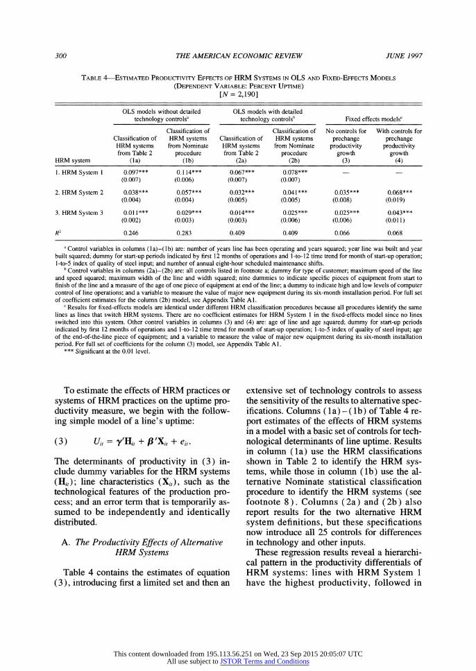
Table 4 contains the estimates of equation (3), introducing first a limited set and then an
extensive set of technology controls to assess the sensitivity of the results to alternative spec- ifications. Columns ( la) - ( lb) of Table 4 re- port estimates of the effects of HRM systems in a model with a basic set of controls for tech- nological determinants of line uptime. Results in column (la) use the HRM classifications shown in Table 2 to identify the HRM sys- tems, while those in column (lb) use the al- ternative Nominate statistical classification procedure to identify the HRM systems (see footnote 8). Columns (2a) and (2b) also report results for the two alternative HRM system definitions, but these specifications now introduce all 25 controls for differences in technology and other inputs.
These regression results reveal a hierarchi- cal pattern in the productivity differentials of HRM systems: lines with HRM System 1 have the highest productivity, followed in
This content downloaded from 195.113.56.251 on Wed, 23 Sep 2015 20:05:07 UTCAll use subject to JSTOR Terms and Conditions

VOL. 87 NO. 3 ICHNIOWSKI ET AL.: EFFECTS OF HR MANAGEMENT PRACTICES 301
order by lines with HRM Systems 2, 3, and 4. F-tests reveal that the difference between the coefficients on HRM Systems 1 and 2 and the difference between the coefficients on HRM Systems 2 and 3 are both significant at the 0.01 level in all models. The estimates of the pro- ductivity effects of HRM systems are very similar in the alternative specifications, al- though the addition of the detailed technology controls reduces the estimated impact of alter- native HRM System 1 by some 3 percentage points.
B. Fixed-Effects Estimates of the Productivity Effects of Alternative
HRM Systems
In estimating the impact of HRM systems on productivity, we want to avoid any pos- sible selection bias arising from nonrandom selection of HRM practices. The ideal data set would be experimental data in which the selection of HRM practices is made ran- domly. However, without an experimental design that ensures random assignment, we must use our nonexperimental data to mimic the desired experimental comparison. In this section we present fixed-effects estimates in light of our concern with nonrandom selec- tion issues.
The most likely reason for the nonrandom assignment of the innovative HRM practices versus the less innovative practices is that "high-quality" lines choose the most inno- vative practices. Thus, we introduce an unobserved line-specific quality variable, ai, in our uptime regression.
(4) Uit = r'Hit + f3'Xit + ai + sit.
Estimates of y in (3) above will be biased if the controls do not adequately incorporate line-specific determinants of productivity that are correlated with choice of HRM systems; that is, if ai ? 0 and E(ai -Hit) * 0. For ex- ample, if the innovative HRM environment exists only in "high-quality" lines (or H1it = 1 if ai > a mjin where aCmin is some threshold value of line quality), then estimates of y are biased if ai is omitted. Because the sample contains longitudinal data and information on
lines that changed their HRM systems, we can control for this potential source of bias with a fixed-effects specification. This can be ex- pressed as:
(5) (Uit - Ui.) (Hit- Hi.)
+ f'(X it- Xi.) + (-itei -)
where the terms subscripted with i indicate line-specific time-series means (for example, Ui. = E_T UijlT).
The fixed-effects results in column (3) of Table 4 eliminate the impact of all fixed line- specific effects (ai ) and also introduce controls for any time-varying productivity de- terminants that were included in the column (2) models. These results document positive effects from introducing more innovative HRM practices: relative to traditional System 4, lines adopting the System 2 set of practices gain 3.5 percentage points of uptime, and lines adopting System 3 practices gain 2.5 percent- age points of uptime.'0
C. A Comparison of Fixed-Effects and Cross-Sectional Estimators
The advantage of fixed-effects estimation is that it controls for any selection bias that would result if different quality lines adopt dif- ferent HRM practices. The disadvantage of fixed-effects estimation is that it uses only the information from HRM "changers" in esti- mating the effects of HRM practices. All cross-sectional information is eliminated in the estimation. Recognizing that the informa- tion from HRM changers is limited because HRM changes are not common events, the data-collection protocol for this study was developed to obtain convincing cross- sectional productivity comparisons. First, we selected a specific production line that would be comparable across different companies. Second, during plant visits we reviewed fea- tures of each line with experienced engineers
0 There is only one set of fixed-effects results because the different methods for measuring HRM systems iden- tify the same set of lines as "HRM system switchers."
This content downloaded from 195.113.56.251 on Wed, 23 Sep 2015 20:05:07 UTCAll use subject to JSTOR Terms and Conditions
302 THE AMERICAN ECONOMIC REVIEW JUNE 1997
to identify technical sources of productivity variation. Finally, we collected the detailed vector of control variables described in Sec- tion I to account for the identifiable sources of productivity variation. If this vector of pro- ductivity controls, Xi,, successfully controls for the line-specific sources of productivity variation that are correlated with HRM choice, then the estimates of y will not be biased by the omission of ai in equation (3), and the coefficients in the fixed-effects results should be comparable to those in the cross-sectional results containing detailed capital controls.
The estimated productivity effects of HRM system variables in the fixed-effects model are virtually identical to those in the column (2b) specifications containing the detailed Xi, con- trols. In particular, t-tests cannot reject the hy- pothesis that the coefficients on the HRM Systems 2 and 3 variables in the fixed-effects model are equal to the corresponding coeffi- cients in the column (2b) model (see footnote 11). As shown in Table 3, no production line switches into HRM System 1, so the column (3) fixed-effects model contains no estimate of the effects of HRM System 1.
Additional specification tests provide fur- ther evidence that the column (2) OLS models already contain a thorough set of controls that adjust for line-specific determinants of pro- ductivity. Not only are the coefficients on the HRM system variables very similar between the fixed-effects and OLS specifications, but the coefficients on the control variables also are nearly equivalent between these two spec- ifications." The Appendix Table Al reports the full set of coefficient estimates for both the
column (2b) OLS specification and the fixed- effects specification.'2
D. Introducing Differential Productivity Growth Rates
The fixed-effects estimators will be inconsis- tent if the adoption of innovative HRM prac- tices is correlated with changes in productivity, such as declining productivity prior to adoption. For example, lines that experience a period of below-average productivity growth may be more likely to adopt new HRM practices. In this case, the estimate of y in the equation (4) fixed-effects model would measure only the ef- fects of adopting new HRM systems for those low-growth lines, and not the effects of new HRM systems for all lines. To control for this possibility, we expand the fixed-effects model to allow the growth rates in uptime to be dif- ferent for lines that switch HRM systems:
(6) (Uit - Ui.)
= - (Hit-Hi.) + f8'(Xit - xi.)
+icP (X - X i) + (sit - i.),
where the two variables in X i are equal to the line age and line age-squared variables for changers measured prior to their HRM change, and are equal to zero at all other times. Thus, coefficient vector W8 represents the differential growth rate in productivity for changers, rel- ative to the base-level productivity growth rate for nonchangers, in 8.'3 The results of esti-
"We calculate t-tests for the hypothesis that the coef- ficients on the Xi, variables in the fixed-effects model are equivalent to the estimated coefficients in the cross- sectional model of column (2b). Each calculated t-test tests whether the difference in the estimated coefficients for the OLS and fixed-effects models is significantly dif- ferent from zero, given the estimated variance-covariance matrices for these two models. We find that the coeffi- cients on the two HRM variables in the fixed effects of column (3) are insignificantly different from their values in the OLS in column (2b), and five of the seven coeffi- cients on the control variables in column (3) are insignif- icantly different from those in column (2b) at the 5-percent level.
2 The coefficients on the control variables in OLS and fixed-effects models are all signed in the expected direc- tion, indicating that lines have more delays with less scheduled maintenance; lower quality steel input; older technologies; start-up periods for brand new lines; the in- troduction of new pieces of equipment; and higher line speeds.
" Equation (6) controls for systematic differences be- tween the average growth rate in uptime for all lines and the growth rate in uptime among HRM switchers over the entire prechange period. An alternative model permits the adoption of a new HRM system to be a function of short- term declines in productivity just prior to adoption. If we reestimate the fixed-effect model and drop an equal num- ber of months before and after the HRM system changes,
This content downloaded from 195.113.56.251 on Wed, 23 Sep 2015 20:05:07 UTCAll use subject to JSTOR Terms and Conditions
VOL. 87 NO. 3 ICHNIOWSKI ET AL.: EFFECTS OF HR MANAGEMENT PRACTICES 303
mating equation (6) are in column (4) of Table 4. The coefficients for this augmented fixed-effects model show somewhat larger ef- fects of changing to HRM System 3 or HRM System 2 than in the column (3) model, in- dicating that lines that switched their HRM systems had somewhat lower productivity growth than average in the periods prior to the adoption of the new HRM systems.'4
Note finally that the standard errors on HRM coefficients may be underestimated due to serially correlated errors. We allow for the possibility of first-order serial correlation of the errors in equation (4) (or sit = Psi(t - 1) + vit) and for first-order serial correlation in the fixed-effects models. When all the models in Table 4 were reestimated allowing for first- order serial correlation, the estimated standard errors increased only slightly. The magnitudes and levels of significance of all estimated ef- fects of the HRM system variables virtually are identical to those presented in Table 4.15
E. The Magnitudes of the Estimated Productivity Effects of HRM Systems
The magnitudes of the estimated effects of HRM systems on uptime are quite consistent across specifications in Table 4. The baseline fixed-effects model in column (3) reports up- time differentials of 2.5 percentage points for HRM System 3 and 3.5 percentage points for HRM System 2, and the estimates from the OLS models with detailed technology controls in column (2) are insignificantly different from these fixed-effects estimates. While fixed-effects estimates for the productivity dif- ferentials for HRM System 1 could not be calculated, the most conservative estimate of the productivity differential for HRM System 1 in any OLS model in Table 4 is 6.7 per- centage points. Are uptime differentials of this magnitude economically important?
Using cost data from one small-scale line, we calculate that a conservative estimate of the effect of a 1-percentage-point increase in up- time on revenues net of any differences in pro- duction cost and any differences in the direct costs of the HRM policies would be approxi- mately $27,900 per month.'6 Using this value, estimates will not be biased by differences in uptime
growth even with serial correlation in the errors (Ashenfelter and Card, 1985 p. 652). We reestimate the model deleting observations for one or two quarters before and after any changes in HRM systems, and the results virtually are the same as those reported in column (3) of Table 4. We suspect that changes in uptime over such short periods would not cause management to adopt new work policies, so we focus on the possibility of longer- term declines in productivity growth.
" We find evidence of a very modest three-month lag in the OLS and fixed-effects uptime models. For example, when the fixed-effects uptime regression [Table 4, column (3)] is reestimated with a lag of three months introduced in the HRM system variables, their coefficients rise by about 0.005 (e.g., from 0.025 to 0.030 for HRM System 3). These lagged HRM variables provide a slightly better description of the changes in productivity due to the new HRM prac- tices than do the concurrent values of the HRM systems. In the fixed-effects model, an F-test reveals that the three- month lags in HRM Systems 2 and 3 add explanatory power to the uptime model already containing the concurrent HRM system variables (F[2,2065] = 3.64), whereas the converse test concerning the addition of concurrent HRM system variables to a model that has the lagged HRM vari- ables is insignificant (F[2,2065] = 1.17).
' 5A further consideration in estimating the productivity models is that the percent uptime variable is bounded by zero and one, suggesting the possibility of Tobit estima- tion. We do not pursue Tobit estimation for the fixed-
effects models because the coefficient estimates of fixed- effects Tobit models are not consistent: the nonlinearity of the Tobit model introduces an incidental parameters problem. However, when the OLS models are estimated as a Tobit with a mass point at one, the estimated coeffi- cients essentially are the same as the OLS estimates pre- sented in Table 4. Note that no lines have uptimes at the mass point of one. A double-sided Tobit with a second mass point at zero is unnecessary since no lines have up- times close to zero.
16 During a delay, a line loses revenue from planned output, incurs fixed costs (which exceed $5000 per hour in some lines) and some "variable" costs such as labor costs, but saves on other variable costs such as the costs of steel and energy inputs. Using a conservative estimate of the profit margin on a ton of steel and liberal estimates of the costs that would not be incurred during a delay, we calculate an increase of $30,000 per month in operating income from a 1-percent increase in uptime. We then sub- tract $2,100 from this figure for the costs of the new HRM policies. We calculate this estimate by using information from interviews to compare the costs of policies in HRM System 1 and HRM System 4. Higher costs of HRM Sys- tem 1 are due to the time production workers must meet off the line, additional HRM staff, consultants for ongoing training and team organization, certain fixed costs of
This content downloaded from 195.113.56.251 on Wed, 23 Sep 2015 20:05:07 UTCAll use subject to JSTOR Terms and Conditions
304 THE AMERICAN ECONOMIC REVIEW JUNE 1997
we conservatively estimate that when one line in our sample changed from HRM System 4 to HRM System 2 and maintained these changes for ten years, it increased its operating profits by well over $10 million dollars strictly as a result of the HRM changes."7
V. Alternative Explanations
The regression coefficients displayed in Ta- ble 4 imply that introducing innovative HIRM systems increases workers' productivity. However, other factors that change over time within lines, such as changes in plant manage- ment or threats of job loss, could be the true cause of the productivity increases. In this sec- tion, we estimate alternative specifications that consider these factors.
A. Management Quality
If better managers are more likely to adopt innovative FIRM systems and to adopt other
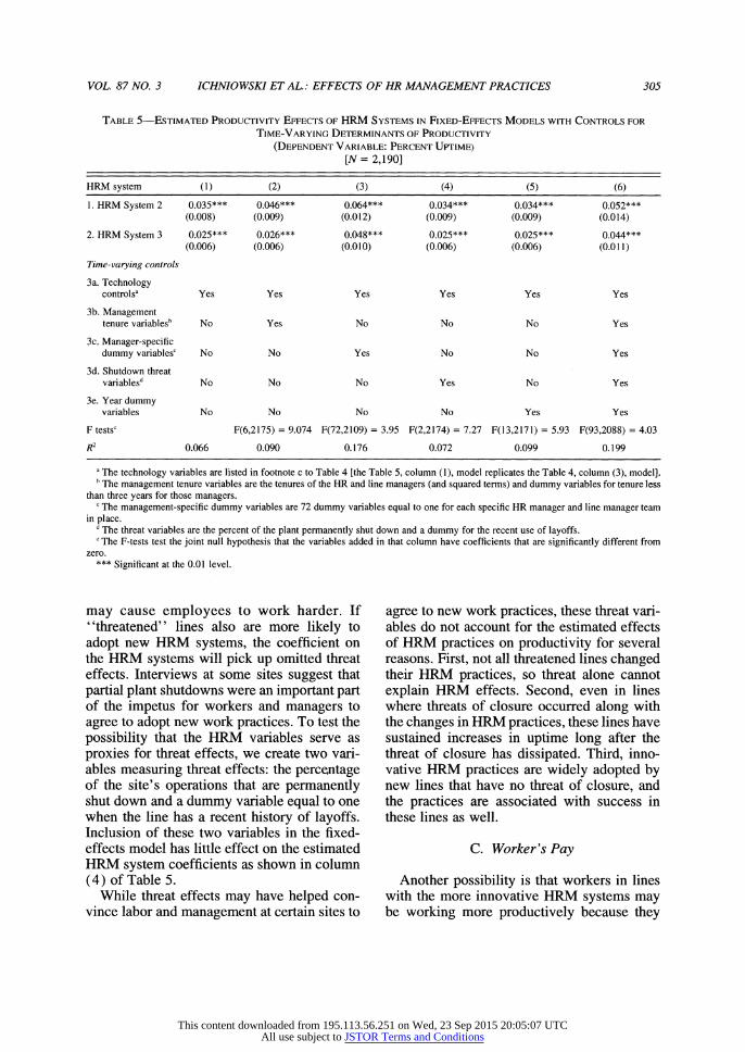
productivity-enhancing practices at the same time, the estimated HRM effects will suffer from omitted variable bias. We collected ad- ditional data to provide two tests of this hy- pothesis. First, we reestimate the fixed-effects model in Table 4, column (3), and include several standard measures of managerial quality-the tenure of the line manager, the tenure of the site's HR manager, and the squares of these tenure variables. We also in- clude two dummies for whether the line has a new line manager or a new HR manager, be- cause the estimated effects of switching HRM systems may only reflect the effects of newly hired managers who change HRM policies upon their arrival. The inclusion of these vari- ables [Table 5, column (2)] produces virtually no change in the estimated HRM system co- efficients relative to our base-model estimates [Table 5, column ( 1 )]. Though only the fixed- effects results are reported in Table 5, results for the OLS model with detailed controls are essentially equivalent to these results for all specifications displayed in Table 5.
These measures of managerial quality may be incomplete if, for example, "good" managers adopt innovative HRM practices and also make other changes to achieve superior productivity. We therefore include in the fixed-effects model 72 person-specific management dummies-one dummy for each period that a line's operations manager and HR manager remained unchanged. As shown in column (3) of Table 5, the inclu- sion of this vector of person-specific manage- ment dummies increases the estimated effects of HRM Systems 2 and 3 compared to the esti- mates from the baseline fixed-effects model in column (1) of Table 5. Overall, the results in- dicate that the effects of the HRM system vari- ables are independent of any managerial behaviors or philosophies that are specific to any individual manager. While higher-quality man- agers may eventually choose to adopt innovative HRM practices, the productivity effects that arise are from the changes in the practices, not from the inherent quality of the manager.
B. Threat Effects
Some lines may face serious threats of lay- offs and plant shutdowns, and these threats
developing these policies, and costs of employment se- curity for wages paid for idle time (assuming that a line would be idle for two months every four years). We allow HRM System 1 to save on the salary of one foreman. As- suming a relatively short time horizon of five years for amortizing fixed costs, the monthly difference in costs be- tween HRM Systems 4 and 1 is about $2,100 per percentage-point gain in uptime. The $27,900 estimate of the monthly revenue increase net of the costs of HRM policies probably is an underestimate because larger-scale lines will have bigger revenue effects, and increases in output quality (discussed in Section V below) yield fur- ther revenue increases.
17 Uptime at this line was consistently some 8 percent- age points higher after the change in HRM systems. The Table 4, column (3), fixed-effects model indicates that 3.5 percentage points of this gain can be attributed to the new HRM practices themselves. Uptime also increased at this line because it began using higher quality steel input near the time of the HRM changes (see Appendix Table Al, column 2, line 5). At $27,900 per percentage point per month, the 3.5-point increase in uptime implies a $1,171,800 annual increase in operating profits and a $12,889,800 increase (without discounting) over the 11 years that this line sustained the improved performance under the new HRM system. Even if this line operated 20 percent below capacity during this period, the change in operating income from a 3.5-percentage-point increase in uptime over an 1 1-year period still would exceed $10 mil- lion. Increases in output quality after this line changed its HRM system further magnify the value of the more pro- gressive HRM systems.
This content downloaded from 195.113.56.251 on Wed, 23 Sep 2015 20:05:07 UTCAll use subject to JSTOR Terms and Conditions
VOL. 87 NO. 3 ICHNIOWSKI ET AL: EFFECTS OF HR MANAGEMENT PRACTICES 305
TABLE 5-ESTIMATED PRODUCTIVITY EFFECTS OF HRM SYSTEMS IN FIXED-EFFECTS MODELS WITH CONTROLS FOR
TIME-VARYING DETERMINANTS OF PRODUCTIVITY
(DEPENDENT VARIABLE: PERCENT UPTIME)
[N = 2,190]
HRM system (1) (2) (3) (4) (5) (6)
1. HRM System 2 0.035*** 0.046*** 0.064*** 0.034*** 0.034*** 0.052*** (0.008) (0.009) (0.012) (0.009) (0.009) (0.014)
2. HRM System 3 0.025*** 0.026*** 0.048*** 0.025*** 0.025*** 0.044*** (0.006) (0.006) (0.010) (0.006) (0.006) (0.011)
Time-varying controls
3a. Technology controls' Yes Yes Yes Yes Yes Yes
3b. Management tenure variablesh No Yes No No No Yes
3c. Manager-specific dummy variables' No No Yes No No Yes
3d. Shutdown threat variablesd No No No Yes No Yes
3e. Year dummy variables No No No No Yes Yes
F tests' F(6,2175) = 9.074 F(72,2109) = 3.95 F(2,2174) = 7.27 F(13,2171) = 5.93 F(93,2088) = 4.03
R 2 0.066 0.090 0.176 0.072 0.099 0.199
'The technology variables are listed in footnote c to Table 4 [the Table 5, column (1), model replicates the Table 4, column (3), model]. h The management tenure variables are the tenures of the HR and line managers (and squared terms) and dummy variables for tenure less
than three years for those managers. 'The management-specific dummy variables are 72 dummy variables equal to one for each specific HR manager and line manager team
in place. d The threat variables are the percent of the plant permanently shut down and a dummy for the recent use of layoffs. c The F-tests test the joint null hypothesis that the variables added in that column have coefficients that are significantly different from
zero. *** Significant at the 0.01 level.
may cause employees to work harder. If "threatened" lines also are more likely to adopt new HRM systems, the coefficient on the HRM systems will pick up omitted threat effects. Interviews at some sites suggest that partial plant shutdowns were an important part of the impetus for workers and managers to agree to adopt new work practices. To test the possibility that the HRM variables serve as proxies for threat effects, we create two vari- ables measuring threat effects: the percentage of the site's operations that are permanently shut down and a dummy variable equal to one when the line has a recent history of layoffs. Inclusion of these two variables in the fixed- effects model has little effect on the estimated HRM system coefficients as shown in column (4) of Table 5.
While threat effects may have helped con- vince labor and management at certain sites to
agree to new work practices, these threat vari- ables do not account for the estimated effects of HRM practices on productivity for several reasons. First, not all threatened lines changed their HRM practices, so threat alone cannot explain HRM effects. Second, even in lines where threats of closure occurred along with the changes in HRM practices, these lines have sustained increases in uptime long after the threat of closure has dissipated. Third, inno- vative HRM practices are widely adopted by new lines that have no threat of closure, and the practices are associated with success in these lines as well.
C. Worker's Pay
Another possibility is that workers in lines with the more innovative HRM systems may be working more productively because they
This content downloaded from 195.113.56.251 on Wed, 23 Sep 2015 20:05:07 UTCAll use subject to JSTOR Terms and Conditions
306 THE AMERICAN ECONOMIC REVIEW JUNE 1997
are paid more. To test this hypothesis, we col- lected wage data from company records and from union contracts (1989 to-1993) and cou- pled these data with interview information to estimate average pay rates.'8 When we include wage rate data, the sample size falls to 863, since the sample is limited to recent time pe- riods. The uptime model is reestimated for this sample with and without the average wage of production workers. The coefficient on the av- erage wage is insignificant in all OLS and fixed-effects models and, therefore, there are no changes in the coefficients on the HRM variables when the wage variable is intro- duced.'9 Factors that are exogenous to the current productivity of the finishing lines de- termine wages.20
D. Other Time-Varying Determinants of Productivity
Finally, we reestimate the fixed-effects specification including a set of year dummies that may be correlated with any omitted time- varying determinants of productivity. Table 5, column (5), reports results from this model. Although the year dummies show a pattern of increasing productivity over time, the effects of HRM System 2 and HRM System 3 are again almost identical to the corresponding co- efficients in the baseline fixed-effects specifi- cation in column (1). Column (6) reports estimated coefficients on the HRM system variables when the fixed-effect model includes year dummies and controls for all other time- varying variables considered in Table 5. The estimated coefficients for the HRM Systems 2 and 3 variables now are somewhat larger than they were in the baseline fixed-effects model of column (1).
In sum, the Table 5 results do not provide any evidence that the coefficients on HRM system variables are biased upward by omitted line-specific or time-varying factors.
E. Effects of HRM Systems on Product Quality
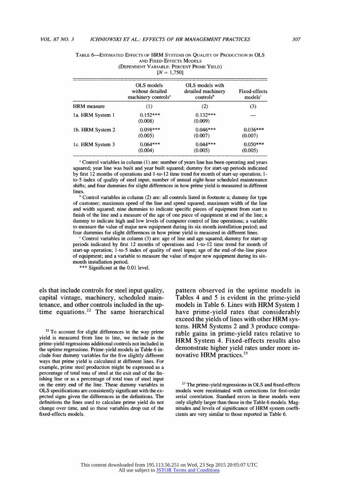
The evidence shows positive significant ef- fects of HRM systems, but the value of these productivity effects will be diminished if they are achieved at the expense of reductions in the quality of output. We collected data on out- put quality as measured by the lines' monthly "prime-yield" rates -the percent of total pro- duction that met the standards for designation as "prime" finished steel. With these data, we are able to test whether the uptime gains re- ported in Tables 4 and 5 are offset by any de- creases in the quality of steel production under the more innovative HRM systems.
Table 6 presents estimates of the effects of HRM systems on prime-yield rates21 in mod-
18 The average wage data for production workers in- clude incentive pay, overtime pay, shift pay, and profit sharing. When these averages were not available for the production line, we used the union labor contracts to pre- dict average wages, combined with interview information on the average grade level, average amount of overtime, and average incentive pay percentages (including profit sharing). Only two lines were unable to provide data for the calculation of average wages. Fringe benefit compen- sation is omitted, and though it is slightly higher in un- ionized lines than nonunion lines due to higher pensions and days off, this omission does not appear to affect the results. First, wages continue to be insignificant determi- nants of uptime when the sample is restricted to unionized lines. Second, union-nonunion differences in fringe ben- efits do not change with the timing of "HRM changers," and wages continue to have no effects on uptime in fixed- effects models.
19 The coefficients (standard errors) on the wage vari- able are 0.00016 (0.00079) for the OLS model with de- tailed controls and 0.00168 (0.00172) for the fixed-effects model. The coefficients on the HRM variables for the sub- sample having wage data (N = 863) are slightly smaller in magnitude than in the full sample, but they remain sig- nificantly different from zero. These results are unchanged when real wages replace nominal wages.
20 Insignificant wage effects are not surprising. First, wage variation in the sample is small. Second, wage changes typically occur when national labor agreements are renegotiated, and these periods do not coincide with systematic changes in productivity. Third, wage changes also do not coincide with changes in HRM systems, so inclusion of the wage variable does not affect the esti- mated effects of HRM systems in fixed-effects uptime models.
2' Because total steel production is the denominator of the prime-yield rate variable, these estimates are not af- fected by any effects of the HRM system variables on production and line delays.
This content downloaded from 195.113.56.251 on Wed, 23 Sep 2015 20:05:07 UTCAll use subject to JSTOR Terms and Conditions
VOL. 87 NO. 3 ICHNIOWSKI ET AL.: EFFECTS OF HR MANAGEMENT PRACTICES 307
TABLE 6-ESTIMATED EFFECTS OF HRM SYSTEMS ON QUALITY OF PRODUCTION IN OLS AND FIXED-EFFECTS MODELS
(DEPENDENT VARIABLE: PERCENT PRIME YIELD)
[N= 1,750]
OLS models OLS models with without detailed detailed machinery Fixed-effects
machinery controlsa controlsb modelsc
HRM measure (1) (2) (3)
la. HRM System 1 0.152*** 0.132*** (0.008) (0.009)
lb. HRM System 2 0.098*** 0.046*** 0.036*** (0.005) (0.007) (0.007)
ic. HRM System 3 0.064*** 0.044*** 0.050*** (0.004) (0.005) (0.005)
a Control variables in column (1) are: number of years line has been operating and years squared; year line was built and year built squared; dummy for start-up periods indicated by first 12 months of operations and 1-to-12 time trend for month of start-up operation; 1- to-5 index of quality of steel input; number of annual eight-hour scheduled maintenance shifts; and four dummies for slight differences in how prime yield is measured in different lines.
b Control variables in column (2) are: all controls listed in footnote a; dummy for type of customer; maximum speed of the line and speed squared; maximum width of the line and width squared; nine dummies to indicate specific pieces of equipment from start to finish of the line and a measure of the age of one piece of equipment at end of the line; a dummy to indicate high and low levels of computer control of line operations; a variable to measure the value of major new equipment during its six-month installation period; and four dummies for slight differences in how prime yield is measured in different lines.
c Control variables in column (3) are: age of line and age squared; dummy for start-up periods indicated by first 12 months of operations and 1-to-12 time trend for month of start-up operation; 1-to-5 index of quality of steel input; age of the end-of-the-line piece of equipment; and a variable to measure the value of major new equipment during its six- month installation period.
*** Significant at the 0.01 level.
els that include controls for steel input quality, capital vintage, machinery, scheduled main- tenance, and other controls included in the up- time equations.22 The same hierarchical
pattern observed in the uptime models in Tables 4 and 5 is evident in the prime-yield models in Table 6. Lines with HRM System 1 have prime-yield rates that considerably exceed the yields of lines with other HRM sys- tems. HRM Systems 2 and 3 produce compa- rable gains in prime-yield rates relative to HRM System 4. Fixed-effects results also demonstrate higher yield rates under more in- novative HRM practices.23
22 To account for slight differences in the way prime yield is measured from line to line, we include in the prime-yield regressions additional controls not included in the uptime regressions. Prime-yield models in Table 6 in- clude four dummy variables for the five slightly different ways that prime yield is calculated at different lines. For example, prime steel production might be expressed as a percentage of total tons of steel at the exit end of the fin- ishing line or as a percentage of total tons of steel input on the entry end of the line. These dummy variables in OLS specifications are consistently significant with the ex- pected signs given the differences in the definitions. The definitions the lines used to calculate prime yield do not change over time, and so these variables drop out of the fixed-effects models.
23 The prime-yield regressions in OLS and fixed-effects models were reestimated with corrections for first-order serial correlation. Standard errors in these models were only slightly larger than those in the Table 6 models. Mag- nitudes and levels of significance of HRM system coeffi- cients are very similar to those reported in Table 6.
This content downloaded from 195.113.56.251 on Wed, 23 Sep 2015 20:05:07 UTCAll use subject to JSTOR Terms and Conditions
308 THE AMERICAN ECONOMIC REVIEW JUNE 1997
F. Why Don't All Lines Have the High- Productivity HRM Systems?
Based on the relative stability of the coeffi- cients in the productivity regressions in Tables 4 and 5, we conclude that the estimated produc- tivity effects of innovative HIRM systems are largely independent of the adoption propensity. However, this conclusion would even be more persuasive if we could identify likely reasons why some lines adopt the productivity- enhancing HRM systems and others do not.
There are two obvious explanations for the limited adoption: (1) managers have had only limited knowledge about the performance ef- fects of IIRM systems; and (2) nonpecuniary barriers to change beyond the direct costs of the work practices limit adoption in certain lines. During our fieldwork at the finishing lines, we found support for both of these explanations.
When most steel mills were built, innovative practices were not in use. However, recently opened lines at "greenfield" sites, as well as older lines that had been closed but were opened with new owners and workers, are adopting in- novative work practices. Knowledge about the potential productivity gains of innovative prac- tices can be considered to be analogous to knowledge about the effects of a technological innovation. While mills at many companies now have some experience with new work practices, many mills still have not adopted the productivity-improving innovation. In particu- lar, continuously operating lines at "brown- field" sites are still much more likely to have traditional HIRM practices.
Our field interviews revealed two sets of reasons for the resistance to the new practices in the older lines despite the growing knowl- edge about the productivity benefits of new work practices. First, managers and produc- tion workers at these sites have irivested in skills and work relationships that would have to change substantially if new HRM systems were adopted. These costs of changing HRM practices do not exist in new lines or in old lines that are reopened by new owners.24 Sec-
ond, the old continuously operating lines are marked by greater mistrust between labor and management, and these lines must overcome this mistrust before the new work practices can be effective.25 The very fact that all of our "greenfield" lines adopted innovative prac- tices suggests that it is the transition costs of adoption that have limited adoption rates.
Different rates of adoption across lines, therefore, are a function of differences in these nonpecuniary costs of adoption that af- fect the profitability of the practices, and not differences in expected productivity gains. In some older lines, new managers or certain workers can champion the new work practices and overcome these impediments to change. In others, credible threats of plant closure mo- tivate existing workers and managers to adopt more productive work arrangements. At the same time, factors like threat effects or work- ers who champion new practices do not appear to be systematic determinants of the produc- tivity effects of innovative FIRM practices. When old lines do overcome these nonpecu- niary costs of switching policies, they experi- ence significant productivity gains from the innovative policies. The variation across lines and within lines over time in these nonpecu- niary costs of adopting new work practices
24 At the same time, the age and older technology of these lines are not responsible for the limited adoption of
new work practices. Detailed controls in the productivity models for capital vintage do not eliminate the productiv- ity effects of HRM systems for several reasons. When older lines in the sample were shut down and later re- opened by new owners, all adopted many new work prac- tices. And, as illustrated by the results of the fixed-effects models, some continuously operating older lines adopted new HRM systems that raised their productivity.
25 Labor-management trust is needed for many inno- vative HRM practices to be effective (Baker et al., 1994). Our interviews revealed how a low level of labor- management trust in older lines rendered ineffective new work practices like information sharing, productivity- improvement teams, and employment security. For ex- ample, the manager at one older line observed: "It's just difficult to change attitudes in old plants with a history of tension and mistrust. We now share financial information with workers, but some workers still believe there are two sets of books." At another line, a supervisor stated: "Workers out here don't believe that they have employ- ment security ... Since employment security is only a con- tractual guarantee, they know that it may very well go away in the next [union] contract."
This content downloaded from 195.113.56.251 on Wed, 23 Sep 2015 20:05:07 UTCAll use subject to JSTOR Terms and Conditions
VOL. 87 NO. 3 ICHNIOWSKI ET AL.: EFFECTS OF HR MANAGEMENT PRACTICES 309
allows us to observe the different work prac- tices in this technologically homogeneous sample, and thus to estimate the impact of al- ternative HRM practices on productivity.
VI. Productivity Effects of Individual HRM Practices
Tables 4-6 show significant positive effects of innovative systems of HRM practices on productivity and product quality. These mod- els do not, however, compare the effects of individual HRM practices to those of systems of practices and, therefore, do not provide ev- idence on whether the individual work prac- tices that comprise an HRM system are complementary. Complementarity among work practices implies that the magnitude of the productivity effect of the system of HRM policies is larger than the sum of the marginal effects from adopting each practice.
In Table 7 we compare the productivity ef- fects of HRM systems with the productivity effects of individual work practices. When variables for individual HRM practices are added to the regressions containing HRM sys- tem dummies, the individual practices have no additional impact on productivity. In other words, the HRM system dummies capture the full productivity impact of the lines' HRM en- vironments; the estimated effect of any indi- vidual HRM practice essentially is zero. Specifically, columns ( la) - ( id) show results from 15 separate productivity models that are the same as the OLS model in Table 4, column (2b), except that each model also includes one additional variable which measures an individ- ual work practice. Similarly, columns (2a)- (2c) show results from models which replicate the Table 4, column (3), fixed-effects model, but each model in these columns also includes one additional variable for an individual HRM
26 practice. 6in nearly all models in the columns
(la)-(ld) OLS models and in the columns (2a) - (2c) fixed-effects models, the coeffi- cients on the variables measuring individual work practices are insignificant.27
Columns (3) and (4) of Table 7 report re- sults from productivity models that introduce only the individual HRM practices without the HRM system variables. The coefficients on the individual practice variables in the OLS and fixed-effects models without the HRM system dummies are positive and significant with magnitudes ranging from about 1 to 3 per- centage points.28 A comparison of the OLS co- efficients in column ( id) with those in column (3) and a comparison of the fixed-effects co- efficients in column (2c) with those in column (4) show that the effects of the individual HRM practices in models without the HRM system dummies disappear once the HRM sys-
26 All OLS and fixed-effects models in Table 7 were reestimated with corrections for first-order serial correla- tion. Again, the magnitudes of all coefficients virtually are unaffected by this correction. Standard errors for some coefficients increase, but only slightly. The significance levels of all HRM coefficients are similar in all cases to those shown in Table 7.
27 While the work practices employed by lines with a given HRM system are highly similar, some work prac- tices do vary within HRM System 3 lines and within the HRM System 2 lines (see Table 2). Furthermore, in ad- dition to the lines that changed enough practices to "switch systems" (see Table 3), other lines change in- dividual HRM policies during the data period. The coef- ficients on the variables which measure individual HRM practices in the OLS estimates shown in column (Id) are positive and significant in only two cases (profit sharing in line 1 and low train in line 10), where the effects still are very modest. As in Table 4, the HRM System 1 vari- able could not be included in fixed-effects models since no line switched into this category with the most innova- tive HRM practices. Also, some fixed-effects models of the effects of individual HRM practices could not be es- timated because certain individual HRM policies do not change in any lines in the sample period. In the fixed- effects models which include the HRM system variables [columns (2a) - (2c)], the only coefficient which is sig- nificantly positive for an individual HRM variable is the coefficient on the low grievance variable (line 15), sug- gesting that productivity-enhancing changes in HRM sys- tems are accompanied by a movement to an environment with little grievance activity, consistent with studies that have found an inverse relationship between grievance ac- tivity and productivity (Ichniowski, 1986).
28 Fixed-effects models which include the multiple teams (line 6) and information-sharing (line 11 ) variables could be estimated in column (4) models without the HRM system dummies because these variables change over time within some lines. However, within-line changes in these two variables are collinear with switches between certain HRM systems, and so the two correspond- ing fixed-effects models in columns (2a) - (2c) could not be estimated.
This content downloaded from 195.113.56.251 on Wed, 23 Sep 2015 20:05:07 UTCAll use subject to JSTOR Terms and Conditions
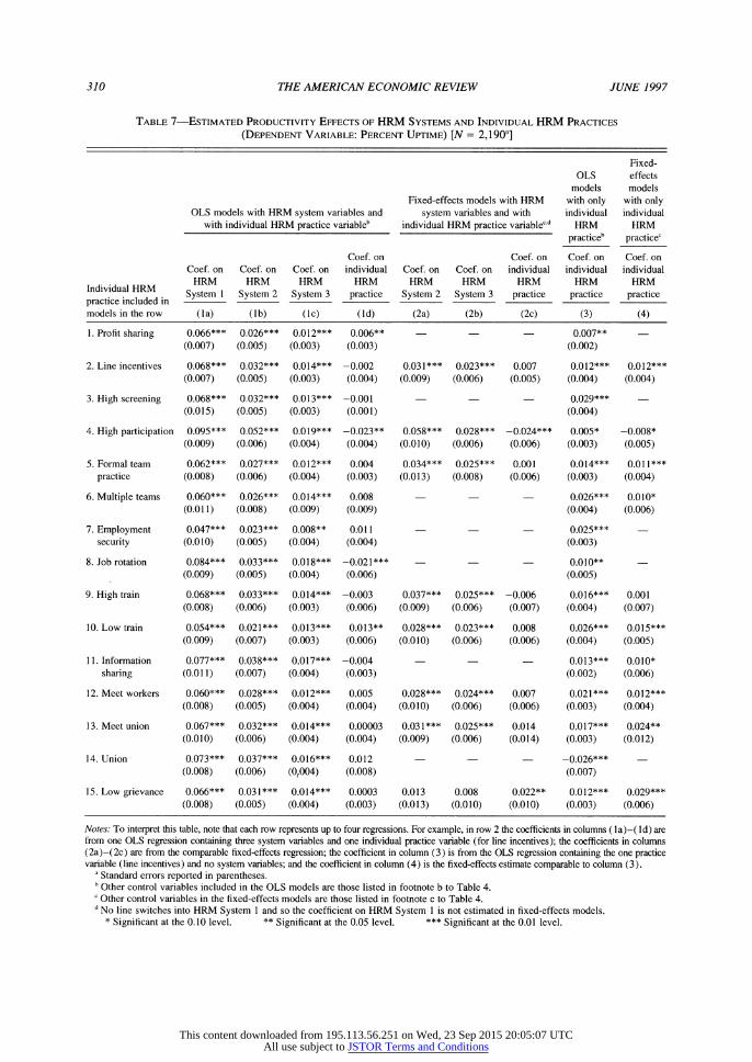
310 THE AMERICAN ECONOMIC REVIEW JUNE 1997
TABLE 7-ESTIMATED PRODUCTIVITY EFFECTS OF HRM SYSTEMS AND INDIVIDUAL HRM PRACTICES (DEPENDENT VARIABLE: PERCENT UPTIME) [N = 2,190a]
Fixed- OLS effects
models models Fixed-effects models with HRM with only with only
OLS models with HRM system variables and system variables and with individual individual with individual HRM practice variable' individual HRM practice variable'd HRM HRM
practice' practice'
Coef. on Coef. on Coef. on Coef. on Coef. on Coef. on Coef. on individual Coef. on Coef. on individual individual individual
HRM HRM HRM HRM HRM HRM HRM HRM HRM Individual HRM System I System 2 System 3 practice System 2 System 3 practice practice practice practice included in models in the row (Ia) (Ib) (Ic) (Id) (2a) (2b) (2c) (3) (4)
1. Profit sharing 0.066*** 0.026*** 0.012*** 0.006** - - - 0.007** -
(0.007) (0.005) (0.003) (0.003) (0.002)
2. Line incentives 0.068*** 0.032*** 0.014*** -0.002 0.031*** 0.023*** 0.007 0.012*** 0.012*** (0.007) (0.005) (0.003) (0.004) (0.009) (0.006) (0.005) (0.004) (0.004)
3. High screening 0.068*** 0.032*** 0.013*** -0.001 - - - 0.029*** (0.015) (0.005) (0.003) (0.001) (0.004)
4. High participation 0.095*** 0.052*** 0.019*** -0.023** 0.058*** 0.028*** -0.024*** 0.005* -0.008* (0.009) (0.006) (0.004) (0.004) (0.010) (0.006) (0.006) (0.003) (0.005)
5. Formal team 0.062*** 0.027*** 0.012*** 0.004 0.034*** 0.025*** 0.001 0.014*** 0.011*** practice (0.008) (0.006) (0.004) (0.003) (0.013) (0.008) (0.006) (0.003) (0.004)
6. Multiple teams 0.060*** 0.026*** 0.014*** 0.008 - - - 0.026*** 0.010* (0.011) (0.008) (0.009) (0.009) (0.004) (0.006)
7. Employment 0.047*** 0.023*** 0.008** 0.011 - - - 0.025*** security (0.010) (0.005) (0.004) (0.004) (0.003)
8. Job rotation 0.084*** 0.033*** 0.018*** -0.021*** - - - 0.010** -
(0.009) (0.005) (0.004) (0.006) (0.005)
9. High train 0.068*** 0.033*** 0.014*** -0.003 0.037*** 0.025*** -0.006 0.016*** 0.001 (0.008) (0.006) (0.003) (0.006) (0.009) (0.006) (0.007) (0.004) (0.007)
10. Low train 0.054*** 0.021*** 0.013*** 0.013** 0.028*** 0.023*** 0.008 0.026*** 0.015*** (0.009) (0.007) (0.003) (0.006) (0.010) (0.006) (0.006) (0.004) (0.005)
11. Information 0.077*** 0.038*** 0.017*** -0.004 - - - 0.013*** 0.010* sharing (0.011) (0.007) (0.004) (0.003) (0.002) (0.006)
12. Meet workers 0.060*** 0.028*** 0.012*** 0.005 0.028*** 0.024*** 0.007 0.021*** 0.012*** (0.008) (0.005) (0.004) (0.004) (0.010) (0.006) (0.006) (0.003) (0.004)
13. Meet union 0.067*** 0.032*** 0.014*** 0.00003 0.031*** 0.025*** 0.014 0.017*** 0.024** (0.010) (0.006) (0.004) (0.004) (0.009) (0.006) (0.014) (0.003) (0.012)
14. Union 0.073*** 0.037*** 0.016*** 0.012 - - - -0.026*** (0.008) (0.006) (0,004) (0.008) (0.007)
15. Low grievance 0.066*** 0.031*** 0.014*** 0.0003 0.013 0.008 0.022** 0.012*** 0.029*** (0.008) (0.005) (0.004) (0.003) (0.013) (0.010) (0.010) (0.003) (0.006)
Notes: To interpret this table, note that each row represents up to four regressions. For example, in row 2 the coefficients in columns (la)-( Id) are from one OLS regression containing three system variables and one individual practice variable (for line incentives); the coefficients in columns (2a)-(2c) are from the comparable fixed-effects regression; the coefficient in column (3) is from the OLS regression containing the one practice variable (line incentives) and no system variables; and the coefficient in column (4) is the fixed-effects estimate comparable to column (3).
Standard errors reported in parentheses. Other control variables included in the OLS models are those listed in footnote b to Table 4. Other control variables in the fixed-effects models are those listed in footnote c to Table 4.
d No line switches into HRM System I and so the coefficient on HRM System I is not estimated in fixed-effects models. * Significant at the 0.10 Ilevel. ** Significant at the 0.05 level. *** Significant at the 0.01 level.
This content downloaded from 195.113.56.251 on Wed, 23 Sep 2015 20:05:07 UTCAll use subject to JSTOR Terms and Conditions
VOL. 87 NO. 3 ICHNIOWSKI ET AL: EFFECTS OF HR MANAGEMENT PRACTICES 311
tem variables also are included. These results from Table 7 demonstrate that the apparent positive effects of individual practices in mod- els without controls for HRM systems are bi- ased by the omission of other HRM practices with which the one included practice is cor- related. New work practices (such as work teams, quality circles, job rotation, or infor- mation sharing) are often introduced together as part of a coherent system of practices; thus, the productivity effects of individual practices cannot be readily isolated.29
To provide further evidence about the pos- sible complementarity of HRM practices, we test whether the interactions among HRM practices that are measured implicitly by the four HRM system dummies are significant when they are added to a regression containing dummies for all the individual practices. Spe- cifically, we reestimate the OLS model corre- sponding to the Table 4, colunm (2b), model, but we include dummies for all individual HRM policies in addition to the HRM system dummies. An F-test rejects the hypothesis that the HRM system variables add no explanatory power to the model that already includes all individual HRM policies entered separately (F[3,2134] = 7.62). Similarly, when we rees- timate the Table 4, column (3), fixed-effects model but include dummy variables for each of the individual HRM policies that change over time in the sample period, an F-test re- jects the hypothesis that the HRM systems variables add no explanatory power to the model (F[2,2142] = 5.40).
The evidence shows that systems of HRM practices determine productivity and quality, while marginal changes in individual work
practices have little effect. The preponderance of evidence in this study also is consistent with the conclusion that complementarities among innovative work practices are important. Note first that the positive correlations among in- novative HRM practices show that firms are likely to select multiple innovative practices rather than single practices, suggestive of complementarities among policies. Second, the productivity regressions reenforce the view that complementarities are important, even though the collinearity among practices inherently limits our ability to distinguish be- tween the impact of individual practices and the impact of systems of practices. HRM sys- tem variables are shown to raise productivity substantially, and the effects of these system variables exceed the effects of the full set of individual practices. Third, in extensive inter- views during our plant visits, operations man- agers offered numerous explanations as to why practices that are introduced in isolation have little effect on performance (Ichniowski et al., 1995 pp. 36-37). Finally, as described in Sec- tion V, subsection F, growing knowledge of the effectiveness of sets of innovative work practices has led steel companies to adopt these practices in all "greenfield" sites, while high transition costs of adopting entirely new systems of work practices have slowed their introduction at "brownfield" sites.
VII. Conclusion
This paper presents new evidence on the pro- ductivity effects of employment practices. The evidence, derived from unique monthly panel data on productivity and HRM practices in a homogeneous sample of production lines, shows that innovative HRM practices raise worker productivity. Moreover, systems of in- novative HRM practices have large effects on production workers' performance, while changes in individual employment practices have little or no effect. Thus, the preponderance of the evidence suggests that, in these steel fin- ishing lines, innovative employment practices tend to be complements, as is proposed in the recent theoretical work on optimal incentive structures. That is, workers' performance is substantially better under incentive pay plans that are coupled with supporting innovative
29 The estimated negative coefficient on union status in the OLS model without the HRM system dummies [Table 7, column (3), line 14] also reflects the more complex dynamics of how systems of HRM policies determine pro- ductivity. On average, union lines are less productive than nonunion lines in our sample. But not all union lines are less productive than the nonunion lines in the sample. The negative union coefficient in Table 7, column (3), line 14, reflects the fact that a large number of union lines have the low productivity practices of HRM Systems 3 and 4, even though the lines in the most productive HRM System 1 are unionized lines. Once the productivity models con- trol for the effect of HRM systems in columns ( la) - ( ld), the union productivity effect becomes insignificant.
This content downloaded from 195.113.56.251 on Wed, 23 Sep 2015 20:05:07 UTCAll use subject to JSTOR Terms and Conditions
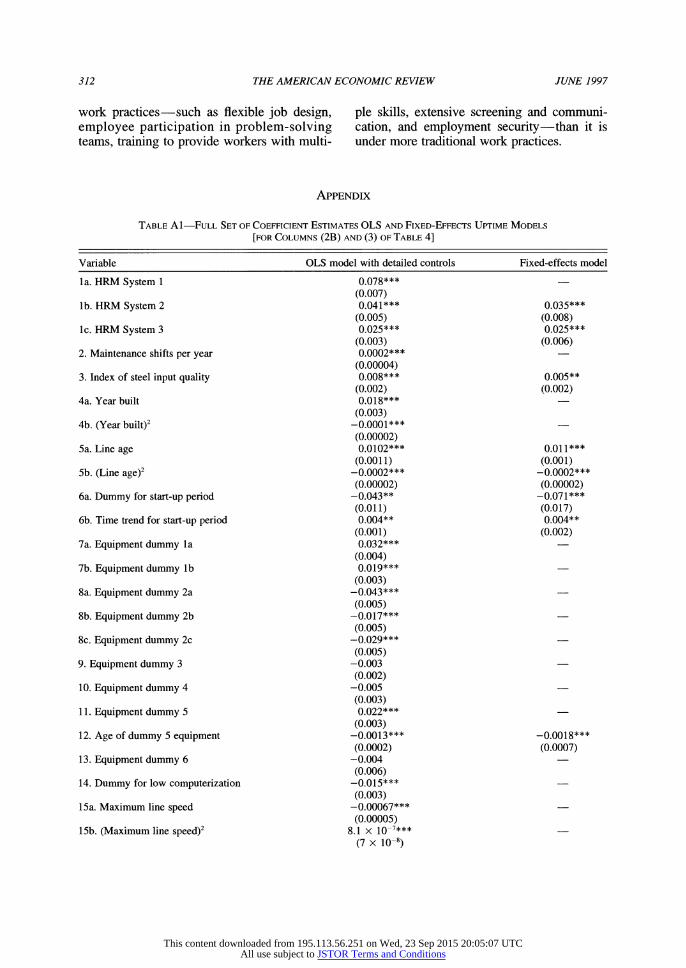
312 THE AMERICAN ECONOMIC REVIEW JUNE 1997
work practices-such as flexible job design, employee participation in problem-solving teams, training to provide workers with multi-
ple skills, extensive screening and communi- cation, and employment security-than it is under more traditional work practices.
APPENDIX
TABLE Al-FULL SET OF COEFFICIENT ESTIMATES OLS AND FIXED-EFFECTS UPTIME MODELS
[FOR COLUMNS (2B) AND (3) OF TABLE 4]
Variable OLS model with detailed controls Fixed-effects model
la. HRM System 1 0.078*** (0.007)
lb. HRM System 2 0.041*** 0.035*** (0.005) (0.008)
lc. HRM System 3 0.025*** 0.025*** (0.003) (0.006)
2. Maintenance shifts per year 0.0002*** (0.00004)
3. Index of steel input quality 0.008*** 0.005** (0.002) (0.002)
4a. Year built 0.018*** (0.003)
4b. (Year built)2 -0.0001*** (0.00002)
5a. Line age 0.0102*** 0.011*** (0.0011) (0.001)
5b. (Line age)2 -0.0002*** -0.0002*** (0.00002) (0.00002)
6a. Dummy for start-up period -0.043** -0.071*** (0.011) (0.017)
6b. Time trend for start-up period 0.004** 0.004** (0.001) (0.002)
7a. Equipment dummy la 0.032*** (0.004)
7b. Equipment dummy lb 0.019*** (0.003)
8a. Equipment dummy 2a -0.043*** (0.005)
8b. Equipment dummy 2b -0.017*** (0.005)
8c. Equipment dummy 2c -0.029*** (0.005)
9. Equipment dummy 3 -0.003 (0.002)
10. Equipment dummy 4 -0.005 (0.003)
11. Equipment dummy 5 0.022*** (0.003)
12. Age of dummy 5 equipment -0.0013*** -0.0018*** (0.0002) (0.0007)
13. Equipment dummy 6 -0.004 (0.006)
14. Dummy for low computerization -0.015*** (0.003)
15a. Maximum line speed -0.00067*** (0.00005)
15b. (Maximum line speed)2 8.1 X 10⁻⁷***
(7 x 10⁻⁸)
This content downloaded from 195.113.56.251 on Wed, 23 Sep 2015 20:05:07 UTCAll use subject to JSTOR Terms and Conditions
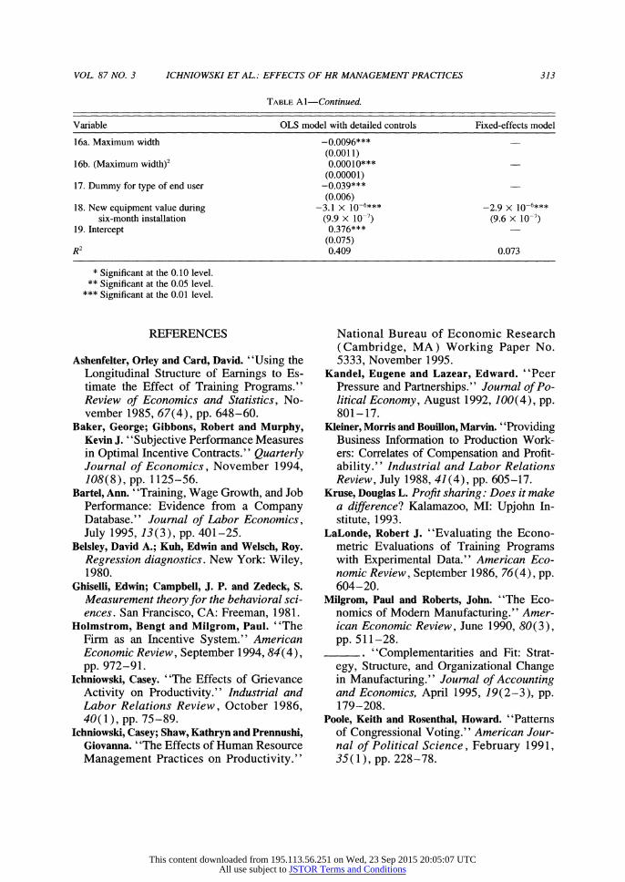
VOL. 87 NO. 3 ICHNIOWSKI ET AL.: EFFECTS OF HR MANAGEMENT PRACTICES 313
TABLE Al-Continued.
Variable OLS model with detailed controls Fixed-effects model
16a. Maximum width -0.0096*** (0.0011)
16b. (Maximum width)2 0.00010*** (0.00001)
17. Dummy for type of end user -0.039*** (0.006)
18. New equipment value during -3.1 x 10⁻⁶*** -2.9 x 10⁻⁶***
six-month installation (9.9 x 10⁻⁷) (9.6 x 10⁻⁷)
19. Intercept 0.376*** (0.075)
R2 0.409 0.073
* Significant at the 0.10 level. ** Significant at the 0.05 level.
*** Significant at the 0.01 level.
REFERENCES
Ashenfelter, Orley and Card, David. "Using the Longitudinal Structure of Earnings to Es- timate the Effect of Training Programs." Review of Economics and Statistics, No- vember 1985, 67(4), pp. 648-60.
Baker, George; Gibbons, Robert and Murphy, Kevin J. "Subjective Performance Measures in Optimal Incentive Contracts." Quarterly Journal of Economics, November 1994, 108(8), pp. 1125-56.
Bartel, Ann. "Training, Wage Growth, and Job Performance: Evidence from a Company Database." Journal of Labor Economics, July 1995, 13(3), pp. 401-25.
Belsley, David A.; Kuh, Edwin and Welsch, Roy. Regression diagnostics. New York: Wiley, 1980.
Ghiselli, Edwin; Campbell, J. P. and Zedeck, S. Measurement theory for the behavioral sci- ences. San Francisco, CA: Freeman, 1981.
Holmstrom, Bengt and Milgrom, Paul. "The Firm as an Incentive System." American Economic Review, September 1994, 84(4), pp. 972-91.
Ichniowski, Casey. "The Effects of Grievance Activity on Productivity." Industrial and Labor Relations Review, October 1986, 40(1), pp. 75-89.
Ichniowski, Casey; Shaw, Kathryn and Prennushi, Giovanna. "The Effects of Human Resource Management Practices on Productivity."
National Bureau of Economic Research (Cambridge, MA) Working Paper No. 5333, November 1995.
Kandel, Eugene and Lazear, Edward. "Peer Pressure and Partnerships." Journal of Po- litical Economy, August 1992, 100(4), pp. 801-17.
Kleiner, Morris and Bouillon, Marvin. "Providing Business Information to Production Work- ers: Correlates of Compensation and Profit- ability." Industrial and Labor Relations Review, July 1988, 41(4), pp. 605-17.
Kruse, Douglas L. Profit sharing: Does it make a difference? Kalamazoo, MI: Upjohn In- stitute, 1993.
LaLonde, Robert J. "Evaluating the Econo- metric Evaluations of Training Programs with Experimental Data." American Eco- nomic Review, September 1986, 76(4), pp. 604-20.
Milgrom, Paul and Roberts, John. "The Eco- nomics of Modem Manufacturing." Amer- ican Economic Review, June 1990, 80(3), pp. 511-28.
. "Complementarities and Fit: Strat- egy, Structure, and Organizational Change in Manufacturing." Journal of Accounting and Economics, April 1995, 19(2-3), pp. 179-208.
Poole, Keith and Rosenthal, Howard. "Patterns of Congressional Voting." American Jour- nal of Political Science, February 1991, 35(1), pp. 228-78.
This content downloaded from 195.113.56.251 on Wed, 23 Sep 2015 20:05:07 UTCAll use subject to JSTOR Terms and Conditions