the effects of automobile safety laws - sam peltzman (journal of political economy, vol 83, no. 4)...

The Effects of Automobile Safety RegulationAuthor(s): Sam PeltzmanSource: Journal of Political Economy, Vol. 83, No. 4 (Aug., 1975), pp. 677-726Published by: The University of Chicago PressStable URL: http://www.jstor.org/stable/1830396 .

Accessed: 25/12/2014 22:01

Your use of the JSTOR archive indicates your acceptance of the Terms & Conditions of Use, available at .http://www.jstor.org/page/info/about/policies/terms.jsp

.JSTOR is a not-for-profit service that helps scholars, researchers, and students discover, use, and build upon a wide range ofcontent in a trusted digital archive. We use information technology and tools to increase productivity and facilitate new formsof scholarship. For more information about JSTOR, please contact [email protected].

.

The University of Chicago Press is collaborating with JSTOR to digitize, preserve and extend access to Journalof Political Economy.

http://www.jstor.org

This content downloaded from 143.106.201.143 on Thu, 25 Dec 2014 22:01:49 PMAll use subject to JSTOR Terms and Conditions

http://www.jstor.org/action/showPublisher?publisherCode=ucpress

http://www.jstor.org/stable/1830396?origin=JSTOR-pdf

http://www.jstor.org/page/info/about/policies/terms.jsp


The Effects of Automobile Safety Regulation

Sam Peltzman University of Chicago

Technological studies imply that annual highway deaths would be 20 percent greater without legally mandated installation of various safety devices on automobiles. However, this literature ignores offsetting effects of nonregulatory demand for safety and driver response to the devices. This article indicates that these offsets are virtually complete, so that regulation has not decreased highway deaths. Time-series (but not cross-section) data imply some saving of auto occupants' lives at the expense of more pedestrian deaths and more nonfatal accidents, a pattern consistent with optimal driver response to regulation.

The attempt to improve automobile safety by regulation of product design is perhaps the trademark of the contemporary "consumerist" movement. The gross and net benefits of this regulation have already been acclaimed.' This paper will first review some of the evidence supporting the acclamations and then proceed to an independent eval- uation of the effects of auto safety regulation. The main conclusion is that safety regulation has had no effect on the highway death toll. There is some evidence that regulation may have increased the share of this toll borne by pedestrians and increased the total number of accidents.

I. Background

Motor vehicle deaths have long been among the 10 leading causes of death, and they usually comprise between a third and a half of all

I am indebted to Paul Evans for diligent research assistance and to Isaac Ehrlich for helpful comments. The support of the Walgreen Foundation for the Study of American Institutions is gratefully acknowledged.

1 See, e.g., any recent Annual Report of the National Highway Traffic Safety Ad- ministration and the summary of benefit-cost comparisons in U.S. Office of Science and Technology (1972). [Journal of Political Economy, 1975, vol. 83, no. 4] ? 1975 by The University of Chicago. All rights reserved.

677



678 JOURNAL OF POLITICAL ECONOMY

accidental deaths. However, the specific role of vehicle design was not a major public policy issue until the mid-1960s, when legislation imposing federal regulation of vehicle design was enacted. While it is overly simplistic to attribute this congressional action to a single source, the widespread attention gained by Ralph Nader's allegations of design defects in the Corvair in his Unsafe at Any Speed appears to have been an important catalyst. Hearings on automobile design began before Nader came to prominence, but the relevant legislation was passed within a year of the publication of his book.

The National Traffic and Motor Vehicle Safety Act of 1966 created what has become the National Highway and Traffic Safety Administra- tion (NHTSA). This agency was empowered to promulgate design standards to which new vehicles sold in the United States had to conform. The first set of these became effective in 1968, and, while they have been subsequently embellished, the 1968 standards remain the most important in terms of their apparent potential for reducing the accident toll. Among the major design changes required by these standards were the following: (1) seat belts for all occupants, (2) energy-absorbing steering column, (3) penetration-resistant windshield, (4) dual braking system, and (5) padded instrument panel. De facto regulation of automobile design apparently preceded these standards, however. Auto producers responded to congressional pressure for legislation by installing many of the devices that became mandatory in 1968. The most significant of these anticipatory moves occurred in early 1964, when front lap seat belts became standard equipment, and in early 1967, when most manufac- turers added energy-absorbing steering columns and penetration-resistant windshields, among other items. Since the market acceptance of these items, except seat belts, was almost nil prior to their becoming standard, it seems reasonable to regard the 1968 standards as mainly a codification of a prevailing regulatory framework.

The specific design changes arising from this regulatory framework reflect some judgments, mostly by safety engineers, about the likely productivity of the various devices. Therefore, I begin by reviewing some of the findings of the safety-engineering literature which produced these judgments.

II. The Promise of Safety Regulation

I shall attempt to provide an estimate of the order of magnitude of the (ceteris paribus) reduction in the highway death rate which the safety literature would lead us to expect following the mandatory installation of safety devices. This involves nothing more than extrapolating the findings from the samples of accidents studied in this literature to the relevant



AUTOMOBILE SAFETY REGULATION 679

population. This exercise is intended to convey some of the rationale for the direction of safety regulation and to provide a reference point for comparison with my own estimates of the effects of regulation.

It is worth pointing out the potential straw-man character of these estimates. In the first place, the approach typical of the safety literature takes the probability of an accident as a datum, and seeks only to measure how much the probability of surviving an accident is enhanced by a safety device. I subsequently elaborate on some of the biases engendered by this approach. Second, I am going to assume initially that none of the devices required by regulation would have been purchased voluntarily. This is perhaps implausible, even though most devices sold poorly prior to their being required. There was, after all, the important exception of lap seat belts. Moreover, the effect of regulation is overstated if, as I argue subsequently, mandated devices substitute in part for safety which would have been purchased without regulation.

Table 1 shows the percentage reduction in the death rate (deaths per vehicle mile) for motor-vehicle occupants which several studies imply we could expect from a few of the devices mandated under the 1966 act. The expected reduction in the total death rate-that is, including pedestrians2 -would be about three-fourths the figures in the table. The estimates are based on 1972 device installation and usage rates. Their sources and derivation are left to Appendix A, but they share some common characteristics. Typically, the studies classify a sample of accidents by outcome to occupants and the presence or absence of a particular safety device, and the productivity is estimated by comparison of mean outcomes (sometimes after an allowance for the interaction effects of multiple devices). In some studies, this estimate is based on researcher judgment that some portion of a sample of accidentfatalities can be blamed on lack of a device.

The main message of the table is that we could expect a reduction of from 10 to 25 percent in the occupant death rate (and 71-20 percent in the total vehicle death rate) from that which might otherwise have occurred in 1972. The "consensus" estimate is closer to the upper end of this range. These estimates reflect a widespread belief among safety researchers about the importance of ejection from a vehicle and impact from the steering column in producing fatalities, as well as the effectiveness of seat belts and energy-absorbing columns in preventing these. For example, Huelke and Gikas (1968) find that the two events produce over 40 percent of fatalities, and their research and related research of Lave and Weber (1970) imply that fully utilized lap belts and an energy-absorbing column would prevent about 70 percent of these deaths. Indeed, the safety literature implies strongly that all that stands in the way of a

2 Who for these purposes include bicyclists and motorcyclists.



68o JOURNAL OF POLITICAL ECONOMY

TABLE 1

EXPECTED REDUCTION IN OCCUPANT DEATH RATE DUE TO SELECTED SAFETY DEVICES, 1972 DEVICE INSTALLATION, AND USAGE RATES

Expected Reduction of Death Rate

Device Source of Estimate (%)

Lap seat belts ........... National Safety Council (1967 et seq.) 7-8-}2 Huelke and Gikas (1968) 13 Levine and Campbell (1971) 16 Kihlberg (1969) 15 Joksch and Wuerdeman (1972) 13 U.S. National Highway and

Traffic Safety Administration (1968) 131 U.S. Office of Science and

Technology (1972)* 14 Energy-absorbing

steering column ...... Lave and Weber (1970) 4 Joksch and Wuerdeman (1972) 5 U.S. National Highway and Traffic

Safety Administration (1968)t Levine and Campbell (1971) 61

Shoulder belt .......... Bohlin (1967) 1 Joksch and Wuerdeman (1972) l Huelke and Gikas (1968) 4 U.S. Office of Science and

Technology (1972)* *

HPR windshield ........ U.S. National Highway and Traffic Safety Administration (1968) 0

Joksch and Wuerdeman (1972) 2+1

Padded instrument panel Lave and Weber (1970) 0

Dual braking system ..... Lave and Weber (1970)

NOTE.-See Appendix A for derivation of estimates. Estimates are rounded to nearest i % for lap seat belts and collapsible steering column, I % for others.

* From Cornell Aeronautical Laboratory data. t From statement by A. Nahum and A. Siegel, University of California, Los Angeles, before U.S. Senate

Commerce Committee, April 25, 1968.

tripled or quadrupled saving of lives is public lethargy in using lap and shoulder belts. 3

Appendix A interprets the relevant data conservatively, so table 1 may understate the effect of these devices. However, even apart from the possibility that some of these devices may have been produced without regulation, there are grounds for skepticism that the productivity of safety regulation is as great as table 1 implies.

Perhaps the most obvious difficulty with these estimates derives from their purely technological character. The mandatory installation of safety devices does not by itself change the private demand for safety, but it may change some relevant prices the response to which may mitigate some of

3 The possibility that seat belts might themselves sometimes be lethal is acknowledged, but dismissed as empirically trivial.



AUTOMOBILE SAFETY REGULATION 68I

A

0 0

0

0 C

0~

Driving Intensity

FIG. 1

the technological promise of these devices. To see this, we may focus on the demand for accident risk on the part of a driver. One need not rely on the dominance of a suicidal impulse to derive such a demand. It would be implicit in any technological complementarity between accident risk and other driving outputs-for example, reduced travel time. The typical driver may thus be thought of as facing a choice, not unlike that between leisure and money income, involving the probability of death from accident and what for convenience I will call "driving intensity." More speed, thrills, etc., can be obtained only by forgoing some safety. The terms of this trade are portrayed, for simplicity, as the ray A in figure 1, where the presumed "bad" probability of death is measured vertically and driving intensity horizontally. Looked at in this way, the effect of making safety devices available (let alone mandatory) is to lower the risk price of driving intensity, that is, to lower the probability of death given an accident. The estimates of the productivity of these devices in table 1 implicitly hold driving intensity constant, and, if C is the ex-device equilibrium, their magnitude would be represented by CD in figure 1. However, if driving intensity is a normal good, we know that the new




equilibrium will be at a point like E rather than D-that is, one at least involving a higher probability of death than at D. Indeed, we cannot rule out a priori a demand for driving intensity so elastic that E involves more risk of death than C.

Such an ambiguity need not, however, derive solely from the belted- milquetoast-turned-daredevil. We have so far ignored another interested party-the pedestrian, or, perhaps, the passenger. There is some complementarity between driving intensity and pedestrian risk, and as long as the new equilibrium entails more driving intensity, we should expect increased risk to pedestrians. This could be offset if the safety devices were designed to reduce all the risks-to drivers and others-of a given level of driving intensity proportionately, but this does not appear to be the case.4 This implication for pedestrians can be generalized: if sufficiently few accidents are prevented by these devices and they lower the probability of death and injury per accident, the induced increase in driving intensity will increase the total number of accidents. A fortiori, the number of accidents involving harm not to occupants but, for example, to property should increase.

The preceding implications followed from associating regulation with an exogenous reduction in the cost per accident, but that cost is also affected by nonregulatory forces. When these are taken into account, some of the implications have to be modified. Consider first an increased private demand for safety.5 For some initially given cost per accident, this increased demand will engender less driving intensity. However, the increased "employment" of accident avoidance raises the marginal productivity of loss reduction. Thus, the market demand for, among other things, safer cars will increase. When producers react to this demand, part of the initial reduction in driving intensity will be offset, since driving intensity is a good as well as a (negative) factor in the production of safety. Thus, increased private demand for safety and safety regulation will both produce lower cost per accident. The qualitative difference, though, is that regulation, to the extent that it is independent of the private demand for safety, will produce a higher equilibrium driving intensity for the same reduction in cost per accident.

That qualitative difference becomes more tenuous in the case of a joint

4 Most of the important devices mandated by the 1966 act are designed to protect occupants after a crash has occurred, though accident prevention has not been completely ignored. The most notable example is, perhaps, the dual-braking-system requirement. There are, in addition, about 20 standards in the so-called 100 Series (accident prevention) of vehicle safety standards which seek to improve lighting and visibility, tire performance, etc.

5 The existence of market insurance will not, in general, eliminate a private demand for either self-insurance (limiting the size of loss) or self-protection (limiting the probability of loss). Indeed, market insurance and self-protection are complements (Ehrlich and Becker 1972).




increase in the demand for safety and intensity. This is perhaps the more relevant case, since it does not require a change of tastes. A rise in real income, for example, would increase the demand for both safety and intensity. While there are different effects, which I discuss later, of wage and time-independent income, there is nothing in general which could lead us to expect a larger income elasticity for either safety or intensity. Therefore, the effects of a rise in income will be similar qualitatively to the effects of mandatory safety devices. There will be a reduced probability of death from any accident as producers respond to the increased demand for safety, and the probability of accident will increase as drivers respond both to their higher incomes and to the reduced probability of death. For a given reduction in probability of death, different quantitative effects of safety regulation and increased income on death rates would then have to rest on the absence of income-induced intensity in the former case.

Some of the preceding points are made more formally in Appendix B, which develops a simple mathematical model of optimum choice of accident likelihood and severity. Specifically, this model implies that more income and more safety regulation are both consistent with (1) reduced severity of accidents (to drivers) for each level of intensity, (2) increased driving intensity, and so increased probability of accident, the net result being that (3) an equilibrium increase in the expected cost (e.g., deaths) from accidents cannot be ruled out in either case.

The similarity of income and regulation effects forces us to question the exogeneity of regulation. The broad trends of income and the death rate are opposite, and this apparent normality of vehicle safety might be responsible for realization of some of the effects in table 1. Even though the market failed to produce the particular devices listed there, this may be more a difference of form (including a shift from accident prevention to loss prevention) than of substance. Put differently, since safety regulation neither increases income nor reduces the price of voluntarily purchased safety, it will lead to some offsetting reduction of such purchases. Whether the offset is partial, complete, or even more than complete then necessarily becomes an empirical matter.6

6 The possibility of a more than complete offset would depend, among other things, on indivisibilities in safety. The basic argument is developed elsewhere (Peltzman 1973) but can be illustrated by an example: Assume that mandated devices yield 100 units worth of safety at the same time the driver demands 150 units worth. Assume further that the cheapest way to produce these 150 units of safety entails a basic change of, say, vehicle design which, in the extreme, must be bought as a bundle or not at all. Thus, the cost of adding 50 units of safety plus that of the 100 the driver is forced to buy will exceed the cost of the design change alone. Under the circumstances, it is conceivable that utility maximization under regulation will dictate purchase of fewer than 150 units of safety. Indeed, the same sort of choice could emerge even if the mandated devices are provided at zero cost to the driver, since the value of 150 units of safety added to the mandatory 100 will generally be less than that of the 150 standing alone.




In summary, there is no clear theoretical basis for expecting safety regulation to be effective or even for predicting the direction of the effect. Therefore, I try to resolve the ambiguity empirically. Specifically, I explore the following issues:

1. Has safety regulation reduced motor vehicle accident deaths? Since a positive answer is sufficient but not necessary for concluding that regulation is effective, I ask:

2. Have nonoccupant injury and death and property-damage accidents increased relative to vehicle-occupant death and injury, and has the probability of an accident increased? These effects are implied if regulation has indeed affected the cost per accident, and the answer to question 1 depends on the relative magnitudes involved in the answer here. A negative answer would imply that safety regulation has ratified market forces, particularly income effects, pushing in the same direction, and not that particular safety devices are technologically ineffective.

To answer these questions, the next section elaborates a simple model of the demand for auto accidents. The parameters of the model will then be estimated from time-series and cross-section data drawn from the period prior to federal regulation of vehicle design. These parameters and the postregulatory values of the determinants of accidents will be used to project the accident rates that could have been expected in the absence of regulation. These projections will then be compared with observed postregulatory accident rates to answer the questions just set forth.

III. The Determinants of Automobile Accidents

I have chosen to view auto accidents as the by-product of an ordinary consumption activity (driving intensity). Therefore, I seek to explain accident patterns as the resultant of forces which shift the demand for risky driving or change the cost of having an accident. This approach involves at least one simplification that should be noted, even if I will ignore it: many accidents involve pedestrians, and the demand for risky walking may differ from that for risky driving.

An analysis of the cost to a driver of having an accident is complicated by the fact that important components of this cost are usually insured. If insurance companies did not adjust premiums in light of particular drivers' accident experience, the insured costs arising from an accident would not deter risky driving. I am, however, going to assume sufficiently accurate and extensive experience rating by insurers for an insured driver to expect to incur some portion of the insured costs associated with his risky driving. If this is so, then the frequency and severity of accidents should be reduced by anything which raises the cost created in an accident. I will represent these costs by an index of direct accident costs (i.e., property damage and medical care) multiplied by an insurance loading factor (the ratio of premiums to benefits paid). That is, if insurance




were simply a method of paying for an accident on the installment plan, the "insured" driver would be liable both for the damage inflicted by an accident and for the cost of administering the collection and payment of these damages; I am assuming that some proportion of these costs is in fact levied against insured drivers. To simplify the empirical work, I am going to ignore the fact that some drivers self-insure and that consequently insurance loading charges may be irrelevant to their behavior.

I have previously argued that income has an ambiguous effect on expected accident costs, since it has opposing effects on the probability of accident and on cost per accident. However, the source of income will affect the relative strength of these effects. Time-related income-for example, wages-is affected by driving intensity. Faster driving, more frequent passing of other cars, etc., increase the hours available for work. Therefore, the same increase in wage rates and income from nonhuman capital will have different effects. Both work to increase the consumption demand for safety and intensity, but the former also increases the demand for intensity as a producer good. A similar difference exists between the effects of increased transitory and permanent wage rates. The former may have small pure consumption effects but will raise the current demand for driving intensity as a producer good, since it raises the shadow price of current leisure. Therefore we should see at least a smaller deterrent effect on deaths from increased wage rates, especially the transitory component, as compared to, say, property income.

To incorporate other variables shifting the demand for risky driving into the model, I rely heavily on the conventional wisdom of the safety literature. Empirical testing of the asserted importance of accident-causing factors could easily tax the available degrees of freedom.7 However, three factors will almost always receive disproportionate attention. These are alcohol, youth, and speed.8 I elaborate briefly on each here and discuss an important offset-highway design-in the next section.

Alcohol

A frequently cited statistic implicates alcohol consumption in over half of fatal accidents.9 The causal inferences drawn from the incidence of significant blood alcohol concentrations among accident victims usually ignore the possibility that some more basic source of demand for risky

7Some of the factors which get more than passing attention are men, small cars, the lack of driver education courses, poor highway design, poorly maintained cars, old cars, bad weather, and skimpy tires.

8 I am, of course, excluding vehicle design here. Some notion of the importance asserted for these factors can be gleaned by perusing almost any of the postwar editions of the National Safety Council's Accident Facts or the NHTSA Annual Reports.

9 See, e.g., National Safety Council (1972, p. 52). However, North Carolina police reports indicate that less than 15 percent of drivers in accidents had been drinking (Highway Safety Research Center 1973).




driving is involved. Indeed, the belief that reduced inebriation will reduce highway accidents has become increasingly institutionalized with the recent spread of implied-consent laws to most states.10

Youth

High relative accident rates among young drivers are as puzzling as they are persistent. If risky driving represents a preference for present as opposed to future consumption, we would expect to find higher accident rates for groups with higher ratios of present to lifetime incomes. Since this ratio generally increases with age, we should find accident rates following the same course. For non-motor-vehicle accidents, this is in fact the case, as the following age distribution of these accidental death rates (per million population) indicates:

Age Group Average 1962-71 Death Rate

15-24 .............. 18.8 25-44 .............. 21.0 45-64 .............. 31.5 65-74 .............. 53.4 75 and older ........ 209.8

The companion distribution of motor vehicle death rates is:11

Age Group Death Rate

15-24 ................ 45.4 25-44 ................ 27.2 45-64 ................ 26.2 65-74 ................ 34.2 75 and older .......... 44.0

Only for the very oldest does the motor vehicle death rate approach that for the young, which exceeds that characteristic of the bulk of the population by over half. This peculiar U-shaped distribution is even more pronounced for drivers in fatal accidents; young drivers are represented about three times more frequently than the safest group (age 50-60).

Since it is beyond the scope of this paper to rationalize the disparity

10 Whereby the cost of a driving license implicitly includes consent to a blood alcohol test on demand of a law officer.

11 Both distributions are from National Safety Council (1973). It should be noted, though, that nonhighway injuries have a similar age distribution to vehicle deaths.




between vehicle and other accidental-death-rate distributions, I will have to treat youth as a "taste" factor raising the demand for risky driving.'2

Vehicle Speed

The ubiquity of speed limit signs and the Safety Council's admonition to "slow down and live" testify to the importance attached to speed as a source of accidents. However, crude evidence for this connection is weak. A large proportion of fatal accidents does involve high speed, but so does a large proportion of all driving. For example, by one recent estimate (National Safety Council 1972) about 60 percent of rural-area fatal accidents occur at speeds over 50 mph, 30 percent at speeds over 60 mph, and 18 percent at speeds over 70 mph. However, counterpart frequencies of rural driving speeds are on the order of 80, 50, and 15 percent. To be sure, these are biased upward,'3 but they surely give scant support to the notion that increased speeds imply increased accident risk. Nevertheless, this notion so pervades the institutions governing driving that I shall want to test its validity. Since I have argued that income and speed are related, the inclusion of income partially provides such a test. However, some of the variation in speed is independent of income, so a complete test requires that the model include this independent component.

The treatment of such things as alcohol, youth, and speed as exogenous sources of demand for risky driving is purely expedient. Surely the driver who wants to take risks can do so more easily with a faster car or by consuming alcohol, and a more complete model of the demand for accidents would treat these, especially speed, as endogenous. However, my specific purpose of estimating the productivity of safety devices will be served as long as there is some reliable connection between more basic sources of demand for risky driving and the proxies I use. For example, suppose the advent of seat belts is accompanied by an increase in alcohol consumption and a fall rather than a-rise in the death rate. In this case, doubt about the implied productivity of seat belts would have to be based on some fortuitous synchronous reduction in the degree of risk that otherwise accompanies drinking. It would appear more reasonable to interpret the increased alcohol consumption as a response which partly offsets the "pure" productivity of seat belts.

It is impractical to treat separately numerous variables which should

12 There is some scattered evidence of interaction between youth and alcohol, in that some surveys have found a higher than average prevalence of significant blood alcohol concentrations among young drivers in fatal accidents (see National Safety Council 1972, p. 52; 1973, p. 52).

13 They pertain to vehicles on main rural roads in off-peak hours in 1971. For secon- dary rural roads, these cumulative percentages are 61, 22, and 3 (U.S. Federal Highway Administration, "Traffic Speed Trends," October 10, 1972).



688 JOURNAL OF POLITICAL-ECONOMY

affect accident rates or severity. Among these would be the state of driver skill, the quality of highways, the private demand and supply of improved vehicle design, the quality of health care, the demand and supply of vehicle maintenance, etc. Some of these factors will respond to driver demand for safety and so should be correlated with income. To the extent that these variables change independently of income, I assume that these can be represented by secular trend. At least the crude death rate data are consistent with a secular increase in safety.

The discussion may now be summarized by writing the reduced form of the model for unregulated accident rates which will be estimated in the next section. This is

R =f (P, Y, T, A, S, K, u), (1)

where R = an accident rate (per vehicle mile) (this will be defined for accidents of differing severity and for all those affected as well as for motor vehicle occupants only); P = the cost component of an accident that is typically insured; Y = income; T = secular trend; A = alcoholic intoxication among the population at risk; S = driving speed; K = driver age; and u = random factors. The expected derivatives are DR/OP < 0, OR/aY(?), OR/IT < 0, 8R/@A > 0, OR/8S > 0, and aR/1K > 0.

IV. Estimates of the Determinants of Accident Rates and the Effects of Safety Devices

This section presents estimates of the determinants of accident rates in the period before federal regulation of vehicle design and uses these estimates to project, for the subsequent period, the rates that could have been expected without this regulation. The effects of regulation are then inferred by comparing these expected rates with actual rates. The comparison is made for both time-series and cross-section data.

Time Series

I developed empirical counterparts to the variables in equation (1) for each year 1947-72. The initial year is chosen to eliminate most of the effects of adjustment from wartime to peacetime driving conditions.14 Prewar data are unavailable for some of the series. I assume that 1965 is the last year that vehicle design was unregulated. This predates the formal imposition of safety standards and treats the sudden ubiquity of lap seat belts in new cars beginning in 1964 as the de facto result of federal

14 It is curious that, in light of the reduced vehicle speeds and numbers of young drivers during World War II, there was a temporary interruption of the secular decline in the death rate in this period.




regulation. (An extra year is allowed for measurable effects of this to show up in the car stock.)

The time series used to estimate equation (1) are as follows: 1. Accident rates (R) each are some measure of damage divided by

vehicle miles driven. The specific numerators employed are for: TDR, the total death rate-all motor vehicle deaths in the United States in the year (sources: 1947-50, National Safety Council [1973]; 1951-72, National Highway and Traffic Safety Administration [1973]); VDR, the vehicle- occupant death rate-total motor vehicle deaths less deaths to pedestrians, bicyclists, and motorcyclists (motorcycles are not treated as "vehicles" because the safety standards we are interested in do not apply to them and their accident rates are atypical of more conventional vehicles; pedestrian deaths typically comprise over 80 percent of those to non- vehicle occupants; source: see TDR); TIR, the total injury rate-total nonfatal injuries due to motor vehicle accidents (source: National Safety Council [various years]); VIR, vehicle-occupant injury rate-total nonfatal injuries less those to pedestrians and bicyclists (source: see TIR; separate data for motorcyclists are not reported); PDR and PIR are nonoccupant death and injury rates, respectively, and are differences between total and occupant rates; DMGR, property damage rate- number of vehicles involved in accidents resulting only in property damage (source: see TIR).

Most of the empirical work is based on rates standardized for type of driving (urban or rural) and type of road (four-lane limited access or other), which are prefixed A, for example, A TDR. This standardization is motivated by the potential inaccuracy of impounding all left-out variables into a trend term. Accident rates differ widely by area (death rates are higher and injury and damage rates lower in rural areas), but there is no clear trend in the urban-rural composition of driving. To remove the influence of shifts in this composition (and conserve a valuable degree of freedom), the adjusted rates are simple averages of urban and rural rates because the postwar averages of urban and rural vehicle miles are roughly equal. Similarly, accident rates are much lower on multilane limited-access roads than any other type (ranging from roughly half as much for death rates down to a tenth for accident rates). Differences among other types of roads are comparatively trivial. However, the safety benefits of limited-access roads are poorly represented by linear trend. Only with substantial construction of the Interstate Highway System in the 1960s does the proportion of total vehicle miles driven on such roads assume any importance. This bunching suggests that a linear-trend model would be better applied to death rates on more conventional roads.15 Such rates are available only for a few recent years, but estimates can be

15 Though this would imply that any gradual improvement in conventional highways was not neglected when the interstates were built.




derived for all years for both urban and rural driving. These estimates are employed in the adjusted accident rates.16

2. The two major components of the cost of an accident, P, which are typically insured are bodily injury and property damage. Given my assumption that a driver can "buy" an accident only at the cost of paying his insurance company some proportion of these and associated administration costs engendered by the accident, I express P as an index of these costs. Specifically, P is a weighted average of the Consumer Price Indexes for physician and hospital costs and auto repair services deflated by the all-items CPI and multiplied by an insurance loading charge. The weights are the proportions of the insurance premium dollar spent on bodily injury (0.4) and property-damage insurance (0.6) over the sample

16 The estimates are derived as follows. For the years 1967-71, death and injury rates as well as vehicle miles and highway miles on interstates and other highways are available in U.S. Federal Highway Administration, Fatal and Injury Accident Rates (various issues). In any year, the adjusted accident rate (AR) for urban or rural driving that we seek is related to the overall rate (R) as follows:

AR= R TVM k . LVM + OVM'

where TVM = vehicle miles driven on all roads, LVM = vehicle miles on limited-access roads, 0 VM = TVM - LVM, and k = ratio of the rate on limited-access roads to that on other roads. Since k is unavailable prior to 1967, I use the average 1967-71 ratio as an estimate for all years. The components of TVM also have to be estimated. To do this, I assume that the ratio of travel density (VM per highway mile) on limited-access highways to that on all highways in any year equals the average 1967-71 ratio for interstate and all roads; separate ratios are calculated for urban and rural roads (and neither show any obvious trend for 1967-71). The resulting estimate of the limited-access density in any year (the 1967-71 density ratio times the all-road density in that year) is multiplied by limited-access highway mileage to obtain LVM, and by subtraction, 0 VM. Unfor- tunately, complete highway mileage data are unavailable, since they are reported by partly overlapping political jurisdictions (state primary systems, Interstate Highway System, and Federal Aid System). For example, a city freeway may be part of the Federal Aid System but neither of the other two, while a toll road may be part of the latter two but not the former. I use the mileage on state primary limited-access roads, since this is usually the largest total. The excluded mileage is bound to be trivial, given the dominant role of the Inter- state Highway System, almost all of which is in state primary systems. The data are available from 1956, when such roads covered only about 1,000 miles compared to over 30,000 currently. I assumed arbitrarily that 600 such miles existed at the end of World War II and that this increased linearly to 1956. However, any reasonable alternative assumption would affect the results trivially. The values of k applied to the resulting LVM series are 0.59 and 0.49 for urban and rural death rates, respectively, and 0.30 and 0.36 for injury rates. The Federal Highway Administration does not report property damage experience. However, National Safety Council (1966, 1967) data on several turnpikes for 1965 and 1966 indicate that property-damage accidents occur twice as frequently as injury accidents on these roads, but 10 times as frequently as on all roads. This implies a k for property-damage accidents one-fifth the 0.34 urban-rural average for injury accidents; I round this to 0.07. (By a similar procedure, the implicit k for property damage is about one-eighth the 0.54 average for death, or also about 0.07.) In general, the road-specific accident rates and the crude rates are virtually identical through about 1960 and then diverge gradually though unevenly. By 1965, the two are something like 5 percent apart for deaths and injuries, and this grows to 10 percent by 1971. The corresponding figures for property damage are double these.




period.'7 The actual insurance loading charge-the ratio of premiums to benefits-is known only ex post, while the expected load should be relevant to the driver's decision. Instead of assuming that drivers have perfect foresight, I constructed a crude approximation to the expected loading charge by dividing this year's premiums by last year's benefit payments. The assumption here is that insurance is bought at the start of the year, at which time both magnitudes are known. (Sources: for price indexes: U.S. Bureau of Labor Statistics [various issues]; for automobile insurance premiums and benefits, 1947-65: U.S. Bureau of the Census, Statistical Abstract [various years]; for auto insurance premiums and benefits, 1966-69: Spectator Co., Property Liability Insurance Review [various years], and A. M. Best & Co. [various issues].)

3. Income, Y, is real earned income per adult of working age (15 and over) (U.S. Bureau of the Census, Survey of Current Business, various issues). This income concept was chosen after a preliminary investigation of several alternatives, which is discussed subsequently. Earned income is estimated disposable personal income from wages, salaries, business proprietorships, and farms (i.e., it excludes transfers, rents, dividends, and interests) (U.S. Bureau of the Census 1966 and Survey of Current Business, various issues).

4. Linear trend is represented by T. 5. Alcoholic intoxication, A, is measured by consumption of distilled

spirits per person 15 years and older (Gavin-Jobson Co. 1974). This excludes illegal consumption, which has been estimated at around 15 percent of the total.

6. Vehicle speed, S, is the estimated average speed of motor vehicles on noninterstate rural roads at off-peak hours (U.S. Bureau of the Census, Statistical Abstract, various years; U.S. Federal Highway Administration, "Traffic Speed Trends," various issues)." Similar data for urban roads

17 In preliminary empirical work, it was found, however, that the results are in- sensitive to a wide range of weights. The medical cost indexes are weighted by relative private expenditures on physician and hospital services averaged over the sample period. The weights are 0.55 for hospital costs and 0.45 for physician fees. The loading charge is earned premiums divided by incurred losses.

18 For purposes of the estimate, personal tax payments are assumed to be the same percentage of each source of income in any year as the percentage of total personal tax liabilities to total personal income less transfer payments that year. Nominal income is deflated by the deflator for disposable personal income.

19 The available data from 1961 to 1969 (U.S. Federal Highway Administration, "Traffic Speed Trends") are for interstate roads (s1) and all roads (st). The estimate for non-limited-access highways (sn) is the solution to

I LVM\ LVM St = tVTVMI + TVM

for the single unknown; TVM and LVM are rural vehicle miles and rural vehicle miles on state primary limited-access multilane highways, respectively. For pre-1961, the 1961 ratio (se/s,) is assumed to prevail in all years. The post-1969 data are spliced to the estimated s,, series.




TABLE 2

REGRESSION ESTIMATES, DEATH RATES, 1947-65

INDEPENDENT VARIABLE DEPENDENT VARIABLE P Y T A S K R2 SE x 100 D-W

A TDR ...... -0.172 0.884 -0.074 0.359 1.843 0.827 .994 1.585 2.080 -1.792 4.317 - 13.900 2.591 3.863 12.232

A VDR ...... -0.045 0.906 -0.068 0.451 2.301 0.594 .978 1.987 1.725 -0.370 3.528 - 10.073 2.592 3.847 7.002

APDR ...... -0.432 0.735 -0.092 0.112 1.016 1.274 .995 2.658 2.247 -2.680 2.140 10.185 0.481 1.271 11.234

NOTE.-See text for sources and description of series. All variables except T are in natural logarithms. The regression constant is deleted. R2 = coefficient of determination; SE = standard error of estimate; D-W = Durbin-Watson statistic (none implies significant autocorrelation of residuals). t-ratios are below coefficients. Since, in natural units, A TDR = A VDR + APDR, the predicted values of one regression should be, but are not, constrained by those of the other two. However, there is almost perfect correlation (around .99) between the constrained and unconstrained predicted values for each series.

are too sparse to be useful.20 7. Young drivers, K, is measured by a proxy, the ratio of the 15-25-

year-old population to those older (U.S. Bureau of the Census, Statistical Abstract, various years [accurate driver-age distributions are available only for a few years]).

A. Death Rates

Table 2 contains estimates of equation (1) for death rates, using earned income per adult as the income concept. Preliminary work with alternative income concepts made it clear that the forces producing a positive relationship between income and the death rate consistently dominated short-run behavior. Every income concept employed had a positive partial correlation with death rates and was coupled with a strong negative trend effect. Apparently much of this short-run behavior is consistent with driver response to changes in the shadow price of leisure. While the speed variable may pick up part of this response, it specifically ignores most commuting traffic and will not capture all risks induced by a rise in the price of leisure (e.g., more frequent passing of other cars). In consequence, as the income concept becomes more dominated by work-time components, its coefficient tends to become more accurate and the explanatory

20 This may not be a serious shortcoming, because the link between accidents and speed is apparently much more important in rural areas. For example, speed is cited as the principal cause on the order of 1, two, and three times more frequently in rural than in urban fatal, injury, and damage accidents, respectively. See National Safety Council (any recent year).




TABLE 3

A TDR REGRESSION RESULTS, VARIOUS INCOME CONCEPTS

t-ratio of SE of Income Regression Estimate

Income Concept Coefficient (x 100)

Per capita permanent income ............ 2.73 1.90

Per capita personal consumption expenditures (proxy for permanent income) ............................ 3.26 1.84

Per capita disposable personal income ..... 3.64 1.75

Disposable personal income per working-age adult ......... .......... 3.73 1.72

Earned income per working-age adult (table 2 concept) ..................... 4.32 1.59

power of the regression increases. Specifically, for the ATDR regression, the results shown in table 3 were obtained. The limited degrees of freedom available made experimentation with much more refined concepts impractical. For example, the table 2 concept implicitly assumes a zero price of leisure for those unemployed or out of the labor force, and does not distinguish permanent from transitory effects. Nevertheless, the fore- going results seem generally consistent with a regime in which the cheapest immediate response to an unexpected increase in income is to increase driving intensity, especially where failure to do so entails a sacrifice of income earning opportunities. (The presumption here is that deviations of income from trend are unexpected.) The strong negative trend effect can then be interpreted as reflecting, in part, a longer-run response to permanent income changes, whereby adjustments of, for example, vehicle design are made to reduce the costs entailed by permanently increased driving intensity. A rationale for such a temporal pattern would be that it simply costs much more relative to the gains to, say, convert immediately a major part of the existing vehicle stock and highway mileage to a safer design than it does to drive the existing stock more intensively.

If the trend term is a partial proxy for permanent income, the regressions seem to imply that the net effect of a (permanent) increase in income is to reduce death rates. That is, the average contribution to death rates from the income term in the regressions is on the order of +2 percent annually and is more than offset by the trend effect. Of course, part of that offset need not be connected with lagged income effects, and more precise estimation of the net effect of income must await discussion of the cross-section data. Since cross-section differences in income tend to be persistent, my interpretation of the time series implies that the coefficient of income should be negative in cross-section data. It also implies a




narrowing of the difference in explanatory power among income concepts. 21

The remaining regression coefficients in table 2 (all of which are elasticities) consistently have the predicted signs and are typically significant. The one important exception is the price coefficient, which is significant only for pedestrian deaths. Alcoholism, speed, and youth also appear to contribute differently to occupant and pedestrian deaths. In the case of the first two, their greater elasticity with respect to occupant deaths is consistent with the highway safety literature. However, the (significant) difference between the driver-age elasticities is surprising. The vehicle-occupant elasticity corresponds closely to the crude difference in death rates among age groups, but the much larger pedestrian elasticity implies that young drivers are peculiarly prone to impose risks on pedestrians.22

The striking size of the speed elasticities should be interpreted cautiously. Taken literally, they would attribute about 40 percent of all current highway deaths to the increase in postwar vehicle speed, and this is over and above the speed effect implicit in the positive income elasticity. 2 However, the same temporal adjustment process may be at work with speed as with income. That is, increased speed may be the most efficient immediate response to increased demand for risky driving, while the loss-prevention expenditures induced by this demand are spread over

21 The behavior of the various income time series reflects a procyclical pattern of trend-adjusted death rates that cannot be rationalized completely on value-of-time grounds. The residuals from the table 2 regressions tend to be highest and lowest at cyclical peaks and troughs, respectively. Attempts to gain further insight into this cyclical behavior proved unrewarding. Specifically, I examined the following: (1) Travel density: The regressions implicitly assume unit elasticity of deaths with respect to vehicle miles. The probability of accident per vehicle mile may increase with density, and this may in turn behave procyclically. However, when density (vehicle miles per highway mile) was added to the ATDR regression, its coefficient was insignificant, though it was positive. (2) New cars: It has been suggested (see "If Economy Crashes, That Could Well Mean Fewer Motorists Will," Wall Street Journal [January 22, 1974]) that increased risk of deaths is a cost of driver familiarization with new cars, sales of which are procyclical. However, the new-car/total-car stock ratio had an insignificant negative coefficient when added to the A TDR regression. One would like to generalize the argument by examining the response to new drivers, but the required data are unavailable. (3) Error in measuring vehicle miles: A spurious procyclical death rate would be produced if the Federal High- way Administration estimate of vehicle miles is smoother than the actual series. However, residuals from a regression of vehicle miles on gasoline consumption were uncorrelated with cycles in income. (4) Driver age: If access of young drivers to the family car is correlated with income, the high accident risk of these drivers will contribute to a procyclical death rate. However, the population death rate for all age categories behaves procyclically. The cycles are slightly more pronounced for the 15-25-year-old group, but this is hardly sufficient to account for much of the cyclicality of the total death rate.

22 It would be interesting to see whether this reflects a more general difficulty in imposing liability for the costs of these deaths on those with low current incomes.

2 3 That is, S will be imperfectly correlated with work-related driving speed because it measures specifically speeds at off-peak hours. I assume that independent variation in work-related speed is correlated with the shadow price of leisure.




TABLE 4

ANNUAL RATES OF CHANGE IN DEATH RATE AND THEIR COMPOSITION, 1948-65 AND SUBPERIODS

SUBPERIOD

VARIABLE 1948-65 1948-54 1954-60 1960-65

ATDR ......................... -1.9% -4.2% -3.1% +2.3% Contribution due to:

T ........................... -7.4 -7.4 -7.4 -7.4

Subtotal (A TDR - contribution of T) .................... +5.5 +3.2 +4.3 +9.7

P ........................... +0.2 +0.2 +0.4 +0.1 Y ........................... +1.9 +2.2 + 1.1 +2.6 A ........................... +0.6 +0.3 +0.6 + 1.0 S ........................... +2.1 +2.6 +1.3 +1.3 K ........................... +0.6 -2.0 + 1.1 +3.2

NOTE.-All percentages are continuously compounded annual rates of change. The "contribution" of a variable is its annual growth rate multiplied by its coefficient in the A TDR regression in table 2. The sum of contributions may differ from the ATDR growth rate due to rounding and random factors. All variables used in the computations are 3-year averages centered about the initial and terminal year of any period. This is done to reduce the importance of random factors.

time and so get reflected in the trend coefficient. Again, the cross-section data will shed some light on the difference between short- and long-run effects of speed.24

The data underlying these regressions may help explain why the political demand for safety legislation increased in the mid-1960s. While the overall trend in the death rate was downward to 1965, the decline slowed in the late 1950s and then reversed itself in the early 1960s. In consequence, 1960-65 constitutes the only period of similar length since the 1920s in which the death rate failed to fall. This fact surely must have contributed to the pressure for safety legislation. In table 4, I try to provide insight into the unique experience of this period just prior to the 1966 act by examining the components of the change in the death rate. Table 4 uses one of the table 2 regressions to partition a change in the death rate among determinants for several subperiods. This partitioning indicates that the most persistent force countering a decline in the death rate was demographic. The favorable effect of a decline in the birth rate in the 1920s and early 1930s had worked itself out by the mid-1950s, and this is sufficient to account for the acceleration of the death rate in the late 1950s. The postwar baby boom then contributed to the subsequent further acceleration of the death rate, so that well over half the acceleration of the death rate from the earliest to the latest postwar subperiod can be attributed to the shift toward a younger driving-age population. How- ever, almost everything else that could have produced an increase in the

24 More light will be shed by results of the national maximum 55 mph speed limit imposed in late 1973.



k :N.5.cc+o v

j

.; cNQoacC w;S;<~-o o .-.- . s ct) m o m d^ (S) Y S - o LO ' o ro r c Ln M- 0 u E M

I I I I I I I I

to S R u o o N o Qo + + + + + + 4 r

;~~~~~~~~~C 0 Q l Lr3Qb r~ 01 -C ul Ln C >1

; g ~~~~~~~~~~~+ -- _ .

_ -. C' en C1 bQ M OU

5~~ ~ ~~~~~~~~~~~ + ? ++++rn + + r@E,

g W * _ ~~~~~0 O Oc O O O Oq O UCXF

CM~~~~~~~~~~~~~~~~~~~~~~~~~~~I

? 2 X I +I I + +

a)) C- r5 CD _ oR

Oj C M en C1 u: C1 C- d<4 C ,,

Lr)~~~ ~ ~ .~ - ,

0 ~~~~~~~~~~~~~~~~~~~~

o . . . . . L. . . . ts '1n

0~~~~~~~~~~~~~~~~~~d0

CC)

. . . . . . . . . 1- C C1_

C14~~~~~~~U u bnVOC)OC M;OW

H ~~~~~~~~~~~~~~~~~'. .0

"0~~~~~~~~~~.

C; C C-i-xi 6 4 ; t- C

C 4

LO C-4~~~~~~~~

- 0

696(DSO~t l z th U 3E

c n C1 n LO cs4 U . _ _ _ _ _ _ _ _ _ ES-e S~~~~~~~~~~~~~~~~~~~~~~~~~~~~~~~~~~~~~~~~~~~~~~~~

696 D :




death rate did so in the early 1960s-the long recovery from the 1960 recession, accelerated growth of alcohol consumption, and accelerated growth of vehicle speeds (the period was marked by popularity of high- horsepower cars).

The early 1 960s experience is important for the present purpose because shortly after the auto producers, under the threat of federal regulation, introduced seat belts as standard equipment, the death rate resumed its secular decline. One interpretation, encouraged by the highway safety literature, attributes this conjunction directly to the new devices. An equally facile alternative interpretation is that the recent experience simply marks a return to a norm which had been well established long before these devices were developed. I try to distinguish among these interpretations by asking how closely the post-1965 experience conforms to that which we could expect from the previous experience. Specifically, if the parameters characterizing the response of accidents to their determinants before 1965 are assumed unchanged and any effect of safety devices is thereby assumed away, how well can we explain the recent experience?

The effects of safety devices on death rates.-To answer this, I use the regressions in table 2 and post-1965 values of the independent variables to generate predicted death rates for recent years. These are shown in table 5 (ignore row 1972a momentarily). If the evidence from safety studies is taken at face value, we would expect the projected rates to exceed the actual by continually widening amounts until a 1972 gap between them approaching perhaps 20 percent was attained. However, no such gap is evident in the behavior of the total death rate (A TDR). Indeed, the projected ATDR tracks the actual rate to within around 2 percent up to 1972, when it falls below the actual by around 5 percent. While this last difference hints at a perverse effect of safety regulation, the standard error of the 1972 regression forecast is too large to permit acceptance of this implication. Virtually identical results were obtained by substituting the unadjusted TDR for A TDR in these calculations (the 1972 TDR exceeds its projected value by 4.1 percent). Finally, I estimated the A TDR regression on 1947-72 data adding the fraction of the car stock of 1964 and later vintage (i.e., subject to federal safety regulation). The coefficient of this variable yields an estimate of the productivity of regulation which should be biased upward.25 However, the bias is too

25 The regression constrains the pre- and postregulatory coefficients to be equal. However, we cannot expect this to be the case generally. Suppose, for example, that with the mandatory devices every increase in income induces a greater increase in driving intensity than without them. In that case, the direct effect of safety regulation as estimated by the coefficient may be favorable, but this would be offset by a higher income effect. A similar argument would apply if safety regulation were simply a particular manifestation of an income effect. The implication of this and analogous arguments shows up in the expanded regression: it has a larger income and driver-age elasticity




small to alter the basic conclusion: the 1972 effect and the t-ratio of the coefficient of the pseudo-proxy for safety regulation are reported in row 1972a of table 5, and both are nugatory. The implication of all this is that there is essentially nothing in the post-1965 behavior of the total death rate that can corroborate the kind of life-saving impact-indeed, any life-saving impact-of safety devices that are adduced in the safety literature. This experience can be explained entirely by the same forces that explain variation in the death rate before these devices became mandatory. 26

To elaborate the details of this conclusion, table 6 presents the composition of the 1965-72 change in death rate along with the companion data from table 3 for 1960-65. These indicate that the recent resumption of the decline in the death rate can be attributed, in order of importance, to (a) a tapering of the influence of the postwar baby boom on the age distribution of drivers, more normal growth of (b) the price of leisure and (c) vehicle speed, and (d) a rise in the price of accidents (insurance loading fees, health care, and auto repair costs have all increased faster than other consumer prices).

Table 5 also contains data on the distribution of highway deaths among vehicle occupants and pedestrians. These can help distinguish among

and a smaller price elasticity than the table 2 counterparts. However, the alcohol elasticities are roughly equal, and the speed elasticity is lower in the expanded regression. This last result implies that the mandatory safety devices are particularly effective in protecting against the effects of high-speed accidents, though the increased income coefficient casts doubt on this implication. On a similar argument, projection of death rates from preregulation parameters may overstate the productivity of regulation. If regulation induces an increase in speed, for example, the projected death rate will be larger than in a pure "no-regulation" world.

26 I am told, by representatives of domestic auto producers, that my results may also reflect failure to account for effects of the recent increase in sales of imports. Most studies show that the probability of death in an accident is higher for occupants of small cars, which until recently were dominantly imports (and vice versa). However, the essential point of this paper is that any such differential probability will induce driver responses working in an opposite direction. When I added the fraction of cars which are imports to the regressions, its effect was insignificant, and some crude post-1965 data tend to confirm this. Among the major industrial states, California and, unsurprisingly, Michigan are at opposite extremes in the receptivity of their drivers toward imports. In the former, the share of imports in total registrations was about 20 percent in 1972 and has grown rapidly in recent years. In the latter, imports account for roughly 5 percent and their share has grown little (the 1972 U.S. average share is about 10 percent). However, no parallel divergence is apparent in recent highway death rate trends. The 1963-65 death rates for the two states are virtually identical (5.1 per 100 million vehicle miles in Cali- fornia, and 5.3 in Michigan), which reflects a basic similarity of driving characteristics. That similarity has apparently dominated their recent experience, because their 1970-72 death rates are still virtually identical (3.9 for California and 4.0 for Michigan). One can also add Illinois to this group, since its drivers have been only a little less hostile to imports than Michigan's. The Illinois death rate closely tracks that of the other two states, falling from 5.0 to 4.0 in the same period. Thus, something like a controlled experiment leaves little room for attributing the lack of effectiveness of safety regulation to the growth of imports.




TABLE 6

ANNUAL RATES OF CHANGE IN DEATH RATE AND THEIR COMPOSITION, 1960-65 AND 1965-71

SUBPERIOD

VARIABLE 1960-65 1965-72

A TDR ......................................... +2.3% -2.2%

Contribution due to: T ........................... .... -7. 7.4

Subtotal (A TDR - contribution of T) ..... .... + 9.7 + 5.2

P ......................................... + 0.1 -0.7 Y ....................................... +2.6 +1.5 A ........................................ + 1.0 +0.9 S ....................................... +2.5 +1.5 K ........................................ +3.2 +1.6

NOTE.-See note to table 4. 1972 values of the variables are used in relevant computations.

rival explanations for the overall lack of effectiveness of safety regulation. If this regulation has not merely ratified market forces, we expect a shift toward nonoccupant deaths, and there is some evidence of this in table 5. Occupant death rates do tend to lie below projected values by increasing amounts over time. If the consistent (though sometimes insignificant) overprotection of AVDR and the significant (biased) coefficient of the regulatory variable in row 1972a lead us to accept the hypothesis that regulation has saved lives of drivers, then the magnitude involved appears to be on the order of half that suggested by a naive reading of the safety literature. At the same time, the preregulation APDR regression consistently underprojects postregulation death rates, and these differences are usually significant. The differences are so large that they engender skepticism, but neither adjustment for growth in bicyclists and motorcyclists (who are included with pedestrians) nor use of a population rather than vehicle-mile death rate changes the basic results.27

27 Bicycle and motorcycle deaths were a growing portion of nonoccupant deaths prior to 1965. If it were assumed that the ratio of these deaths to other nonoccupant deaths maintained its pre-1965 growth rate (about 3 percent annually), and that none of its recent acceleration was due to substitution for pedestrian deaths, then the 1972 APDR would have been about 5 percent lower than it was. The use of vehicle miles to deflate nonoccupant deaths assumes implicitly that driver action "causes" them. At another extreme, we could assume that pedestrians seek risk independently of driver action, vehicle density, etc. In that case, population, as a proxy for the number of pedestrians seeking risk, would be the more appropriate deflator. However, when the figures in table 5 are obtained from a regression using a population death rate, the underprojection of post-1965 death rates actually becomes more severe (by about 10 percentage points). The reason is that vehicle miles have some effect on pedestrian deaths, and their growth has accelerated relative to population in recent years. Finally, use of unadjusted death rates reveals the same shift in the incidence of risk as the adjusted data. The projected PDR is 26 percent below the actual, and the projected VDR is 5 percent above the actual in 1972.




TABLE 7

REGRESSION ESTIMATES, INJURY AND PROPERTY DAMAGE RATES, 1947-65

INDEPENDENT VARIABLE DEPENDENT VARIABLE P Y T A S K R2 SE x 100 D-W

A TIR ....... -0.249 0.524 -0.067 0.295 2.224 0.670 .983 2.190 3.010 - 1.770 1.807 -9.203 1.524 3.473 7.050

A VIR ....... -0.220 0.503 -0.064 0.399 2.594 0.469 .957 2.502 2.882 -1.371 1.516 -7.635 1.803 3.546 4.318

APIR ....... -0.290 0.318 -0.096 -0.322 1.624 1.574 .993 4.010 1.738 - 1.128 0.598 -7.147 -0.908 1.386 9.041

ADMGR -0.515 0.818 -0.069 0.466 1.663 0.527 .960 2.891 1.473 -2.938 2.190 -7.070 1.843 1.912 4.271

NOTE.-See note to table 2 and text.

The time series data then imply that safety regulation has not merely reflected market forces, for then its failure to reduce the highway death rate should have been matched by failure to change the distribution of these deaths. The safest inference from the time series, though, is that there has been a shift in the burden of accident risk toward nonoccupants, which is consistent with optimal driver response to an exogenous reduction of the expected loss from an accident. I will examine injury and property-damage experience and some independent evidence on driver behavior for corroboration of this inference.

B. Injury and Property Damage

Effective regulation should also lead to a substitution of less for more severe accidents. Some of these will substitute injury for death, while others will substitute property damage for injury. While one cannot therefore predict the net effect on total injuries, pedestrians should, as with deaths, bear a larger share of the burden of injuries. And we should observe a net increase in property-damage accidents.

Regression estimates of equation (1), with injury and property-damage rates as the dependent variables, are presented in table 7. These are subject to much more measurement error than death rates.28 However,

28 This is due to the greater degree of underreporting and subjectivity of definition involved with the less severe accidents. The resulting problems are well illustrated by a comparision of the National Safety Council injury series, which I use here, with an alternative series produced by the Travelers Insurance Company: the two are not in remote agreement about either the level or rate of change in motor vehicle injuries. The Travelers estimate of total injuries is currently about 21 times that of the safety Council, though the immediate postwar excess was only about 30 percent. In recent years, the Federal Highway Administration has also collected injury data, and these run roughly at the geometric mean of the other two series! The Safety Council is the sole source of property accident estimates, but these are bedeviled by sporadically changing reporting requirements, and are consequently rounded generously.




the regressions almost suspiciously mirror their counterparts in table 2, most notably in their lack of much residual variance. If there are any notable differences between the two sets, they might be the generally lower income elasticity for the less severe accidents and the larger price elasticity of damage accidents.29 In view of the close correspondence between the different accident series prior to safety regulation,"3 it would be surprising if their behavior differed much subsequently.

The postregulatory injury rate experience does mirror that of death rates. The important exception is injury rates for vehicle occupants. The projections from the AVIR regression in table 7 (see table 8) are usually below the actual values, though the differences are insignificant. Similarly, the coefficient of the fraction of cars subject to regulation in the expanded form of that regression is insignificant (row 1972a). Therefore, the weak evidence in favor of reduced occupant deaths due to regulation does not hold up for injuries. However, there is evidence for harmful injury effects on pedestrians of roughly the same magnitude as for death rates. However, since the vehicle-occupant series dominates the total, we cannot safely conclude that total injury rates have been adversely affected by regulation. 31

Table 8 also compares projected and actual property-damage accident rates. These series behave differently from both death and injury rates, and in precisely the way we would predict if safety regulation has been at all effective: there are significantly more damage accidents after regulation than could have been expected. The size of the gap is startling. Both of the estimates for 1972 imply an excess of on the order of 4 million damage accidents.32

The overall thrust of the time-series evidence is then consistent with a regulation-induced reduction in the probability of death per accident,

29 The last result seems reasonable if the fraction of an accident's cost which the insurer imposes on a driver varies inversely with its amount. However, in that case the price elasticity of injury accidents should exceed that for fatalities, but it does not.

30 The correlation between any pair of accident rates is typically above .95. 31 Some independent evidence indicates that injury accidents as a whole have become

more severe in the aftermath of safety regulation. From 1958 to 1964, a period in which alcohol consumption, speed, and demographic trends were unfavorable, the average paid auto insurance claim for bodily injury deflated by the price index for medical care actually declined by 0.6 percent per annum. From 1964 to 1971, in an environment otherwise less conducive to injury, the average claim increased 2.1 percent per annum. (Data are from Insurance Information Institute [various years].)

32 The unadjusted demage rates behave similarly; the actual rate exceeds the projected rate by .264 (natural log units) in 1972. Moreover, there appears to be a subsidiary effect here similar to that encountered with pedestrians: damage accidents have become more damaging. From 1958 to 1964, the average paid auto insurance claim for property damage, deflated by the auto repair price index, rose 2 percent per annum. It will be recalled that vehicle speed, alcohol consumption, and demographic trends in this period were all conducive to increased property damage. Their force abated subsequently, but the increase in the average damage claim accelerated to 6 percent per annum from 1964 to 1971. (Data are from Insurance Information Institute [various years].)



k o e0 CN4C1 LO CN4 LO) 00r

.00 -CoC - OCoO * -4 -4 ~ (i vi ce

0 0 t- - CO CO . 1 M C1 co - sC14c

S~~ ~~~ + + +++ +++

LoQ I t - LO w- LnOoo m COC-4" CNCN

*--4

^

p.4

0 m CD O mXOc m Ln0 0LOLO LO~ Q

~

0 0 m ~c 0)C1 C

:s - t- -. CO C.

.S. .JCNNNX

~~~~~~~C'I t- - C, r- r- ?mo

u)^~~~~~N Q m-4 -4 - NN

O~~~~- cq- * 0 M m t- r

. p

19 C-4 _ D 0) N _ o o 0 co 4 P., Cs! co0 C m N CO 0 C ___

k *oooooooo

:~~~~~C - -: oo.N4 6s6 C

Z Q + + + + +I +I

Q (CewjN(COnCOL

o V V C

4-j

* ?4

p44

M CC LO C14 (c LO -C~4 0 (c C14 -

V --*oo-o-o-oc

> ~~+++ I +

.4q oR CR lC

I-dR c'i

C) c ++ ++I++++

4- L~ nM . )- OML

&4 v)

- CLo r- C --- 0

V C4 -

C CM M -

0

LO(Cr~~~~cCO)0-CNCN~~~r C

,Q

C) r~060 CMC C9NCMC1---

o; ow cm aN ao

702




to which drivers have responded with more risk taking. It is this response to which I have attributed the conjunction of (1) an unchanged death rate, (2) an increased risk of death and injury for nonoccupants, and (3) an increased probability of property-damage accidents. I examine next some more direct measures of driver risk taking for consistency with the preceding interpretation.

C. Driver Risk Taking

While increased risk taking by drivers can take many forms, the time- series regressions tend to confirm the importance of those associated with alcohol, age, and speed, especially the latter two. Therefore, if safety regulation has led to increased risk taking by drivers, this might be manifested in higher driving speeds, more young drivers, and increased inebriation among drivers. After these conjectures are tested, I shall examine data on accidents to cars of specific model years.

To examine the effect of regulation on driving speed, I first estimated the following regression on preregulation data (1947-65):

S = Constant + 0.013 T + 0.109 Y - 0.210 PG - 1.311 IM (4.535) (1.262) (-2.819) (-2.618)

R2 = .988, SE = 0.75 x 10-2, D-W = 2.327

(t-ratios below coefficients), where, in addition to symbols defined previously, PG = log of the consumer price index for gasoline divided by the all-items CPI (per mile gas consumption increases with vehicle speed), and IM = ratio of imports to the total stock of cars (imports typically have lower speed capability than domestic cars). I then projected values of S for the postregulation period, 1966-72, from this regression to see whether they fell short of the actual values. In fact, however, the projected and actual values are consistently within 1 or 2 percent of each other, so we must reject the hypothesis of a regulation- induced increase in vehicle speed. The same result is obtained by adding the fraction of cars subject to regulation to a regression on 1947-72 data. The coefficient of the variable is less than one-tenth its standard error.33

Another way that safety regulation may lead to increased probability of an accident is through reduced inhibition of driving by the young. Unfortunately, preregulation data on the age distribution of drivers is

3 3Legal costs may be an important left-out variable here. Speed limits increased little in the 1960s, so that actual driving speeds began to bump against legal limits by the end of the sample period. The average state-noninterstate speed limit has hovered around 60 mph since 1960. In 1960, only 20 percent of all cars were exceeding this speed. This doubled by 1965, but was only about 50 percent by 1972 (see U.S. Federal Highway Administration, "Traffic Speed Trends"). This slowing may reflect the nature of the traffic laws which tax speed only above a critical level which many drivers are beginning to crowd.




TABLE 9

RATIO OF DRIVERS TO NONDRIVERS BY AGE, 1958, 1965, 1972

CHANGE OF RATIO FROM DRIVERS/NONDRIVERS EARLIER YEAR (%)

Under 25 25 and Older Under 25 25 and Older SERIES AND YEAR (1) (2) (3) (4)

National Safety Council: 1958 ................... 2.88 2.13 ... ... 1965 ................... 2.66 2.99 - 7.6 +40.3

Federal Highway Administration: 1965 ................... 2.91 3.01 ... ... 1972 ................... 3.42 4.16 + 17.5 +38.2

NOTE.-Prior to 1965, the National Safety Council was the sole source of data on the age distribution of drivers. From 1965 on, the Federal Highway Administration had published similar data (see U.S. National Highway Traffic Safety Administration 1973). The figures in col. (1) are adjusted to account for the effects of lower driver participation of those under 20 and shifts in the age composition of those under 25. Specifically, the ratio of drivers to population (P) is calculated separately for the age cohorts 16-19 and 20-24 in each year. These are combined into a weighted average (i) with fixed weights of .478 and .522, which are the 1958-72 average proportions of these subcohorts in the 16-24 cohort. The figures in col. 1 are P/(l - X). The unadjusted data for col. 1 would be 2.90, 2.65, 2.86, and 3.46 reading from top to bottom. Percentage changes are for data from the same source.

sketchy, so they must be interpreted cautiously. However, it is possible to trace the propensities of different age groups to drive through two periods of equal length centered about initiation of safety regulation. This is done in table 9, and the data do imply some reduced restraint on driving by the young after the onset of regulation. Specifically, while driver participation (as measured by the ratio of drivers to nondrivers) among those over 25 increased at roughly the same rate in the two periods, participation among the young accelerated after 1965. This may help explain the substantially increased pedestrian risk which we found for this period, since the regression in tables 2 and 7 indicate that pedestrians are peculiarly vulnerable to young drivers.

Data on arrests for drunkenness also appear to be consistent with a postregulation increase in driver risk taking. Table 10 compares trends in arrests for drunkenness, drunk driving, and all other "minor" crimes. The series share inaccuracies from changes in coverage, but with the onset of regulation there is a marked departure from the previous con- formity of drunk-driving arrests to arrests for other types of drunkenness. Both arrest rates had been declining in tandem, while the arrest rate for other minor crimes remained roughly unchanged. Specifically, the pre- 1965 correlation of the two drunkenness arrest series is .91. After 1965, this correlation becomes strongly negative, and arrests for drunk driving grow much more rapidly than for other minor crimes. The divergence between the two drunkenness arrest series can be reconciled by intro- ducing safety regulation. When the drunk-driving arrest rate for the whole 1953-71 period is regressed on that for other types of drunkenness and the fraction of the car stock subject to safety regulation, the partial correlation between the two arrest series (.89) is hardly different from the




TABLE 1 0

ARREST RATES FOR DRUNKENNESS, DRUNK DRIVING, AND OTHER NONSERIOUS CRIMES,

SELECTED YEARS

CHANGE OF ARREST ARREST RATES (PER 1,000) RATE IN PERIOD (%)

Other Nonserious

Drunk Drunkenness Crimes Driving (per Person (per Person Other

(per 15 and 15 and Drunk Nonserious YEAR Driver) Older) Older) Driving Drunkenness Crimes

1953 4.45 23.81 22.20 ... ... ... 1959 3.85 21.69 24.59 -13.5 -9.1 + 10.7 1965 3.53 16.60 23.11 -8.3 -23.4 -6.0 1971 5.75 13.32 29.30 +62.9 -19.8 +26.8

NOTE.-Data are from U.S. Federal Bureau of Investigation (various years). Prior to 1960, data are available for urban areas only. Therefore, pre-1960 rates are estimates obtained by multiplying reported arrests by the 1960-61 ratio of total to urban arrests. Reported arrests were divided by population in the areas covered by the FBI survey (pre-1960 population is estimated in a manner similar to arrests) and multiplied by the national ratios of population to the relevant subgroup. See source for definition of nonserious crimes. Drunkenness and drunk driving are separate subcategories.

earlier-period simple correlation (but, of course, much greater than the full-period simple correlation, which is .47), and the partial correlation of drunk driving with regulation is highly significant (.91).

Interpretation of these data as reflecting an increase in the demand for risky driving is, however, subject to an important qualification. The onset of safety regulation coincides with an increased spread of "implied consent" laws, which make it easier for police to obtain evidence of driver intoxication. At the same time it is worth noting that annual growth of alcohol consumption has roughly doubled since 1965, so it risks exaggeration to attribute all of the reported increase in drunk driving to legal changes.

Canada and North Carolina accident data.-Safety regulation in Canada has basically paralleled that in the United States, beginning with "voluntary" introduction of lap belts in 1964. It is therefore possible to use some Canadian data, which classify cars involved in accidents by model year, to test the hypothesis that regulation induces increased driver risk. That hypothesis implies that cars subject to regulation will have above- average accident frequencies.

It will be expedient to focus on the ratio of cars from model year m to all cars reporting involvement in an accident in year t (RAmt).34 To

34 The data are too fragmentary to permit development of an analogue to the regressions in tables 2 and 7 for each vintage of car. Some relevant independent variables are unavailable for Canada. More important, the model-year breakdown of accidents covers selected provinces, and the coverage is not uniform over time. Therefore, I do not seek to explain the absolute level of accidents in any year's sample, but rather the distribution of accidents among model years. The data are from Statistics Canada (various years).




isolate the impact of regulation on RA, I will take account of the effects of the ratio of cars from m to the total car stock in t (RCmt), and the age of cars from m in t (Vmt). The latter variable is included as much to standardize for reporting differences as to measure a true age effect: accidents involving older cars more frequently fail to meet minimum damage criteria for reporting. The basic regulatory variable (SRm) uses the information from table 1 that lap seat belts produce about 60 percent of the total expected productivity of safety devices. It is defined as zero if m is before 1964, 0.6 for m from 1964 to 66, and 1.0 for 1967 and later vintages. The effect of regulation on any one vintage's share of accident involvements will become diluted as cars subject to regulation become more common, because of both simple arithmetic35 and the increased probability that preregulation cars will be struck by postregulation models. As the latter approach ubiquity, the effect of regulation on any one vintage's share of the higher accident total will vanish. To develop a linear approximation to this process, we may let B * SRm be the partial effect of regulation on RAmt, where B is a coefficient. However, that coefficient should decline as the fraction of the car stock subject to regulation (FR,) rises; B can then be expressed as Bo + B1 * FR,, so that the partial effect of regulation becomes Bo * SR. + B1 * (SRm * FR,). We would expect Bo > 0, B1 < 0, and, more precisely, Bo = IB11 (so that the partial effect vanishes when FR = 1).

The results of the regression on Canadian data fulfill these expectations. The regression is

RAmt = 6.65 + 0.59 RCmt - 0.54 Vmt (11.14) (-13.00)

+ 2.07 SRm - 2.14 (SRm * FRt) (3.24) (-2.15)

R2 = 0.92, SE = 0.89

(t-ratios are below coefficients, RA and RC are in percentage point units). The sample consists of vintages 10 years old and less (which usually comprise about 90 percent of the total stock) for years 1959-72, or 140 observations,36 of which 45 are subject to regulation. The interesting result, of course, is that the coefficients of the regulatory and interaction variables have the sign pattern and the (virtual) equality of absolute

3 For example, suppose that the car stock consists of v equal-sized vintages, of which k are regulated. If x is the probability that a car from any of the k will be involved in an accident andy the probability for a preregulatory car, RA will be xl[kx + (v - k)y]. This will be I/v if x andy are equal, but it must approach I/v as k approaches v even if x exceedsy.

36 In some cases, the original accident data were for groups of vintages. For these, I allocated the group total among vintages in proportion to the vintage share of cars. This procedure therefore biases the coefficient of RC toward unity and overstates its accuracy.




value which is consistent with a regulation-induced increase in driver risk taking. The magnitude of the coefficient of SR is also of interest. It implies that if the sample-average vintage (8.75 percent of the car stock and 9 percent of accidents) is made subject to regulation, its accident frequency increases fully 25 percent. This is sufficient to offset the reduction in deaths per accident claimed by the safety literature for mandated safety devices, and it is well within the range of my estimate in table 8 of the regulation-induced excess accident frequency for the United States.

Further corroboration of the time-series results and of increased accident frequency for postregulation cars may be found in North Carolina accident data. Levine and Campbell (1971) use a sample of North Carolina accidents occurring in 1966 and 1968 to cars built in 1964 and after, classified by presence or absence of an energy-absorbing steering column (and implicitly the group of other devices introduced simultaneously; all cars in the sample have seat belts). North Carolina car registration data (R. L. Polk & Co., various years) indicate that no more than 27 percent of all cars eligible for the sample in the 2 years were equipped with this safety device. However, cars so equipped account for 34 percent of all accidents in the sample. That is, the probability of an accident involving cars with the safety devices is 40 percent greater than for cars not so equipped.37 This is more than sufficient to outweigh the reduced risk of death per accident to drivers of such cars (14 percent in this study), and even suggests that the large estimates of increased accident risk in table 8 are conservative.

In summary, then, the fragmentary evidence is broadly consistent with some increase in driver risk taking since implementation of safety regulation. At the least those data implying such an increase are countered by none showing the opposite. I next examine cross-section death rate data to see whether they reveal the same impact of this increased risk taking on the level and distribution of death rates as the time series.

Cross-Section Data

The impact of the Highway Safety Act has been spreading gradually as pre-1964 cars are replaced with subsequent vintages. Because the rate of replacement varies among areas, so will effective enforcement of the act. This cross-sectional variation in effective enforcement of the Safety Act provides an opportunity to test the effectiveness of safety regulation.

Essentially, I will ask whether death rates are lower in areas (states) where cars with safety devices are more prevalent. As with the time series, I will want to account for nonregulatory influences on death rates, so I

3 7But, from the Canadian data, about half of this excess may be due to underreporting of accidents by unequipped, older cars.




proceed as follows: Assume that the cross-section distribution of the death rates (D) in a year subsequent to the onset of regulation is generated by

Dt = aXt + bRt + ut, (2)

where X = matrix of nonregulatory determinants of D, R = matrix of variables serving as indices of the effective degree of enforcement of regulation, a, b = vectors of coefficients, and u = a random variable. In practice, R will be related to the age distribution of cars. For example, in 1970 safety regulation had affected all cars 6 years old or less, so R might be measured by the fraction of all cars of 1964 or later vintage in a state. Now, one wants to allow for the possibility that the age of cars may exert an influence on D independent of regulation.38 Therefore, it is insufficient merely to estimate equation (2) on data for year t. To dis- entangle the effects of car age and regulation, then, suppose that in some earlier year, t - i, D is given by

Dt-i = a'Xt-i + b'Rf-i + ul (3)

where R' is defined analogously to R. That is, if R1970 is the fraction of cars built from 1964 to 1970, then R'960 would be the fraction of cars built from 1954 to 1960. Then, if regulation has no effect, a and b would equal their earlier counterparts (ignoring nonstationarities). If regulation does have an effect, it could change a' as well as b'. By analogy with the time-series tests, we can impose the constraint a = a' and then see if we must reduce b' to successfully explain D. That is, if we assume that Dt is generated by the same process as Dt-i and regulation has in fact altered the process, we should be overpredicting death rates where R1970 is high and mutatis mutandis. In general, then, we can define

b = b' + B. (4)

where B is a change induced by regulation. So, equation (2) could be rewritten

Dt = aXt + b'Rt + BRt + Ut. (5)

Then, imposing the constraint on a, compute

Vt = (Dt - a'Xt - b'Rt), (6) and then estimate

Vt = BRt + ut. (7)

If regulation effectively reduces the death rate, an estimate of B should be negative. Equations (3)-(7) summarize the basic procedure I use to

38 Though experiments with the time series suggest the effect is weak. In addition to the experiment with the new-car variable reported in n. 21 above, I conducted one using average age of car as an explanatory variable. Its coefficient was insignificant.




test the effects of regulation, though modifications (for example, of the implicit assumption that u' and u are uncorrelated) will be treated.

Since the cross-section data differ in some respects from the time series, it is useful first to summarize the nature and rationale of these differences 39

the dependent variables are accident losses per capita rather than per vehicle mile (denoted, e.g., A TDC for the total death rate). Accurate state vehicle-mile data are unavailable prior to the last several years, but a fairly good proxy, highway fuel consumption, is available. Rather than constrain the vehicle-mile elasticity of fuel consumption to be one, I make per capita fuel consumption (FC) an independent variable.

Per capita death rates are adjusted to remove effects of interstate highway travel, but not the urban-rural driving mix. Some states have so little driving of one or the other type that a simple average of urban and rural death rates would be unrepresentative of the local experience. However, to account for urban-rural death rate differences, the ratio of urban to rural driving (U/R) is entered as an independent variable. Further, since urban and rural driving conditions are not uniform across states, I employ rural and urban densities (RD, UD)-that is, vehicle miles per highway mile-as independent variables. The effect of density on the death rate is somewhat complex, however. Everything else being the same, we would expect increased density to increase the probability of an accident and thereby death. However, increased density discourages fast driving, passing on two-lane roads, etc., and on this account would reduce deaths.

Estimates of vehicle speed are unavailable for all states, so I use as a proxy the speed limit on main (non-limited-access) rural roads (SL). In preliminary work with a subsample, the residual from the regression of estimated vehicle speed on SL proved uncorrelated with death rates, perhaps in part because these speed estimates sometimes behave erratically over time. Therefore, the characterization of vehicle speed in a state is left to the set of variables SL, U/R, UD, RD.

The price of an accident proved singularly difficult to estimate, primarily because cross-section indices of medical care and auto repair prices are unavailable. I assumed that these were correlated with wage rates for hospital personnel and automechanics, respectively, and employed indices of these as proxies for prices. A weighted average of these indices multiplied by an insurance load is then used as the cross-section accident price variable (PA). One would like to deflate PA by a cross- section general price index, but this too is unavailable. In consequence, PA will inevitably vary with local wage and salary levels.

The cross-section data permit us to measure both the long-run response

39 A detailed description of the sources and methods of constructing these data is available from the author.




of death rates to income and any differences in response to earned and unearned income. Instead of a single income measure, then, I enter disposable personal income per capita (YD) and the ratio of earned income per adult to unearned income per capita (E/N). If my interpretation of the time-series evidence is correct, YD, which would be dominated by permanent cross-section income differences, should have a negative coefficient (or one at least smaller than its time-series counterpart) while the coefficient of E/N should be positive.

Both alcohol consumption (A) and the age distribution of the population (K) are measured as in the time series. The former of these uses local liquor store sales, but tax differentials stimulate considerable interstate movement of liquor purchases, and this introduces measurement error in A.

The basic data are for 1961-71, but to reduce the importance of random components, triplets are averaged to yield four cross sections centered about 1962, 1965, 1967, and 1970. The notation Xt, then, always refers to a 3-year average centered about t. To provide a reference point for subsequent work, table 11 presents cross-section regression estimates for the various death rates with regulatory variables excluded. These differ in some respects from the time-series results, so a brief summary of results is useful.

Speed.-The singular importance of this variable carries over to the cross-section data, as does the differential importance for vehicle occupants and pedestrians. In fact, the magnitudes of the time-series and cross-section speed elasticity estimates are almost the same. For fragmentary data on actual vehicle speeds, the cross-section elasticity with respect to SL is on the order of 0.3-0.4, and when these are divided into the coefficients in table 11, the implied actual speed elasticities correspond roughly to those in table 2.

Urban-rural driving and densities.-The cross-section data mirror the persistent excess of rural over urban death rates, especially (indeed exclusively) for vehicle occupants. However, strong density effects show up in urban areas and for pedestrians. That is, the discouragement of risky driving provided by high densities appears to dominate the behavior of drivers in rural areas.

Alcohol.-The time-series and cross-section data disagree on both the overall importance of alcoholism and its relative impact on pedestrians and drivers. Indeed, the subgroup alcohol elasticities here are very nearly the reverse of those in table 2.

Youth.-Perhaps the most glaring contradiction between the time- series and cross-section data occurs here. There is virtually no evidence in table 11 of the substantial age differentials in the death rate that show up in crude data and the time-series regressions, nor is there much evidence of a differential impact on pedestrians. Since age differentials in the death rate are pronounced in every state (see Iskrant and Joliet 1968), it



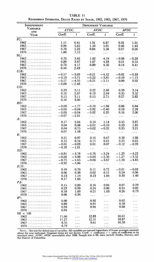
TABLE 11 REGRESSION ESTIMATES, DEATH RATES BY STATE, 1962, 1965, 1967, 1970

INDEPENDENT DEPENDENT VARIABLE VARIABLE A TDC A VDC APDC

AND YEAR Coeff. t Coeff. t Coeff. t

FC: 1962 ............... 1.11 6.41 1.31 6.87 0.32 1.31 1965 ............... 0.94 5.65 1.10 5.91 0.40 1.43 1967 ............... 0.70 5.22 0.84 5.58 0.07 0.26 1970 ............... 1.00 7.15 ... ... ... ...

SL: 1962 ............... 0.76 3.42 1.02 4.19 -0.09 -0.29 1965 ............... 0.89 3.97 1.07 4.33 0.21 0.55 1967 ............... 0.73 4.17 0.89 4.50 0.14 0.41 1970 ............... 0.44 2.43 ... ...

U/R: 1962 ............... -0.17 -3.69 -0.21 -4.12 -0.02 -0.33 1965 ............... -0.19 -3.71 -0.22 -3.81 -0.10 - 1.15 1967 ............... -0.17 -4.55 -0.21 -5.11 0.00 0.02 1970 ............... -0.09 -2.48 ... ... ... ...

UD: 1962 ............... 0.23 3.11 0.22 2.68 0.33 3.14 1965 ............... 0.16 2.67 0.13 2.04 0.35 3.52 1967 ............... 0.15 3.11 0.15 2.71 0.27 2.82 1970 ............... 0.16 3.06 ... ... ... ...

RD: 1962 ............... -0.09 -1.77 -0.10 -1.94 0.06 0.84 1965 ............... -0.00 -0.04 -0.02 -0.40 0.18 2.28 1967 ............... -0.00 -0.04 - 0.02 0.35 0.16 2.06 1970 ............... -0.07 -2.01 ... ... ... ...

A: 1962 ............... 0.17 2.04 0.10 1.14 0.45 3.87 1965 ............... 0.04 0.48 -0.01 -0.10 0.23 1.85 1967 ............... 0.04 0.75 -0.02 -0.32 0.35 3.21 1970 ............... 0.07 1.18 ... ... ... ...

K: 1962 ............... 0.21 0.97 0.16 0.67 0.58 1.88 1965 ............... 0.12 0.54 0.15 0.61 0.25 0.65 1967 ............... -0.01 -0.03 0.01 0.07 -0.12 -0.33 1970 ............... -0.18 -1.01 ... ... ... ...

YD: 1962 ............... -0.81 -3.78 -0.76 -3.24 -1.29 -4.23 1965 ............... -0.66 - 3.08 -0.60 -2.50 - 1.27 -3.52 1967 ............... -0.75 -4.65 -0.66 -3.67 - 1.50 -4.85 1970 ............... -0.92 - 5.06 ... ... ... ...

E/N: 1962 ............... 0.10 0.70 0.11 0.72 -0.01 -0.03 1965 ............... 0.06 0.38 0.02 0.11 0.24 0.96 1967 ............... 0.13 1.14 0.13 1.04 0.30 1.40 1970 ............... 0.17 1.66 ... ... ... ...

PA: 1962 ............... 0.15 0.89 0.16 0.84 0.07 0.29 1965 ............... 0.23 0.93 0.24 0.86 0.35 0.82 1967 ............... 0.18 1.00 0.21 1.03 0.26 0.73 1970 ............... 0.06 0.34 ... ... ... ...

R2:

1962 ............... 0.90 ... 0.92 ... 0.62 ... 1965 ............... 0.89 ... 0.91 ... 0.59 ... 1967 ............... 0.93 ... 0.94 ... 0.68 ... 1970 ............... 0.94 ... ... ... ... ...

SE x 100 1962 .11.66 ... 12.83 ... 16.61 ... 1965 ............... 11.27 ... 12.51 ... 18.87 ... 1967 ............... 8.55 ... 9.61 ... 16.50 ... 1970 ............ .. 8.73 ... ... ...

NOTE.-See text for definitions of variables. All variables are natural logarithms of 3-year averages centered about the year indicated. Constant terms are not shown. Coeff. = coefficient. t = ratio of coefficient to its standard error. A VDC, APDC unavailable after 1968. Sample size is 48; data exclude Alaska, Hawaii, and the District of Columbia.




is difficult to believe that age is really a proxy for something left out of the regressions, and the cross-section results for age merit skepticism.40

Price of accident.-This variable has no significant impact on death rates in any cross section, but this may reflect the peculiar difficulty of measuring cross-section price differences.

Income.-The cross-section results provide a clue to the large negative secular trend terms in the time-series regressions. The income elasticities in table 11 are uniformly negative and significant, in sharp contrast to those in the time series, but consistent with dominance of long-run income effects in the cross sections. If one assumes that the cross-section elasticities measure long-run adaptations while the time-series elasticities capture short-period effects, the difference between the two elasticities would account for something like half of the time-series trend coefficients. The algebraically lower cross-section elasticity for pedestrian as opposed to occupant deaths is also consistent with the time series. Both short- and long-run income changes apparently lead to a substitution of driving for walking. Finally, there is some weak evidence that the differential response to earned and unearned income that was found in the time series is permanent. The coefficient of the ratio of these incomes is persistently positive, though never significant."4

The Effect of Safety Regulation

The primary test for the effectiveness of safety regulation entails the addition of a variable like R' in equation (3) to an appropriate table 11 regression, computation of a variable like V in (6), and an estimate of B in (7). Estimates of B, which should be negative if regulation has

40 These results are influenced by interesting cross-section differences in the impact of age. The ratio of the 18-24-year-old to total death rate tends to be lower where that group is relatively large (e.g., the South and West). See Iskrant and Joliet (1968). This may reflect adaptation by localities to the magnitude of the relevant risk through, for example, police enforcement and driver training programs. A successful reconciliation of the cross-section and time-series data would require an explanation of these differences in age-specific death rates.

41 Attempts to refine measures of the income effect proved unrewarding. For example, I broke each state's per capita income into linear-trend and deviation-from-trend components in a crude attempt to distinguish "permanent" from "transitory" effects. However, there was no significant difference between the coefficients of these components. With similar motivation (and results), I added the interperiod change in income to the regressions. The income effect in the cross sections, like the trend effect in the cross sections, undoubtedly summarizes a number of forces, and, given the larger degrees of freedom, I attempted to measure the effects of some of these separately. However, this attempt was also unsuccessful. It entailed addition of, among others, the following variables to the regression: (1) state highway police expenditures for traffic law enforcement (unfortunately, local enforcement authorities do not account separately for this function); (2) state highway department road expenditures; (3) the availability of hospital care, as measured by hospital beds per highway mile; (4) the percentage of cars which are imports; and (5) education, as measured by median years of schooling.




TABLE 12

EFFECT OF REGULATION ON DEATH RATES, AS MEASURED BY COEFFICIENT OF

FRACTION OF CARS IN A STATE SUBJECT TO REGULATION

PERIODR COEFFS. COEFFICIENT/t-RATIO FOR REGULATORY VARIABLE

RESIDUAL FOR A TDC A VDC APDC (Dependent PREDICTED Variable) DR B B' CHG B B' CHG B B' CHG

1970 ...... 1962 0.47 0.56 0.43 ... ... ... ... ... ... 1.49 1.96 1.37

1970 ...... 1965 -0.25 -0.19 -0.02 ......... ... ... ... -0.94 -0.82 -0.09

1970 ...... 1967 -0.68 -0.64 -0.24 ... ... ... ... -2.71 - 3.02 -1.29

1967 ...... 1962 1.51 1.60 0.54 1.96 2.03 0.57 0.83 1.01 0.97 2.78 3.22 1.00 3.23 3.66 0.93 1.10 1.66 1.42

1967 ...... 1965 0.65 0.64 0.10 0.88 0.85 0.21 0.45 0.43 0.09 1.64 2.26 0.30 2.00 2.71 0.59 0.62 1.03 0.21

1965 ...... 1962 1.41 1.54 0.74 2.18 2.22 0.64 -0.45 0.30 1.74 1.40 1.87 0.77 1.96 2.36 0.56 -0.31 0.23 0.85

NOTE.-DR residual is the difference between a death rate in the year indicated and the death rate predicted using coefficients from a regression in some prior year. The specific prior year is that in the column headed "Coeffs. for Predicted DR." Each column labeled B contains the coefficients (over ratios to their standard errors) of a variable constructed from the ratio of cars produced after regulation to the total stock of cars in a regression with DR residual as the dependent variable. In the construction of the independent variable, each car with seat belts only (1964-66 models) is weighted 0.6, and 1967 and later models are weighted 1.0. Data are from R. L. Polk & Co. (various years). Each column labeled B' contains a counterpart to B in a regression which includes the residual from the prior-year regression as an independent variable. The column labeled CHG contains counterparts to B and B' in a regression where the change in death rates is the dependent variable and changes in independent variables in table 11 are included. Coefficients of nonregulatory variables and summary statistics for regressions have been deleted. See text for illustration of variable construction. A VDC, APDC are unavailable for 1970.

reduced death rates, are in table 12. The meaning of these estimates can be clarified by focusing on a specific case. In the first line of the table, we want to know if the 1970 death rate was reduced by safety regulation. Now, in 1970 all cars built since 1964 were subject to regulation. However, those built since 1967 had more substantial design changes, substantial enough, table 1 suggests, to improve on the life-saving potential of a 1964-66 model by perhaps two-thirds. Therefore, I define a variable equal to 0.6 x number of 1964-66 cars + 1.0 x number of 1967-70 cars all divided by the total stock of cars as the measure of the impact of regulation (R) in 1970. Since R also measures the age of cars, I then construct an analogue (R') for 1962, and add it to the set of variables in

the 1962 A TDC regression in table 11. Data for 1970 are then plugged into this expanded 1962 regression to generate a predicted death rate for 1970. This variable tells us what the 1970 A TDC would be if it had been generated by the same process as the 1962 ATDC. When this predicted 1970 A TDC is subtracted from the actual, we obtain a "residual" which includes any impact of regulation. For if regulation in fact altered the 1962 process, this residual should be smaller the larger the variable R; that is, the coefficient of R in a regression of the residual on R should be




negative. This coefficient is reported under B in the table (ignore B' momentarily).

Since there is some sampling fluctuation in the table 11 coefficients, we can check for consistency of the regulation effect by generating predicted values of the 1970 A TDC from alternative table 11 regressions, specifically those for 1965 and 1967. Here the R' variable will include some impact from regulation, but always less than R.42 Therefore, the predicted sign of the R coefficient remains negative if regulation is effective. Similarly, tests can be conducted on 1967 and 1965 death rates by suitably redefining the R variable.

The main conclusion to be drawn from table 12 is the same as from the time series: regulation appears not to have reduced highway deaths. Given the preponderance of positive coefficients, one might be tempted to blame regulation for an increase in deaths, but the general lack of sig- nificance of the coefficients and their erratic behavior precludes such a conclusion. The time pattern of the coefficients is also inconsistent with effective regulation. For any year's death rate, the contrast with the earliest alternative year should yield the algebraically smallest regulation coefficient (since the later alternatives are affected by regulation); just the reverse is true for both 1970 and 1967. The generally lower 1970 coefficients hint that the set of devices mandated after 1966 (energy- absorbing column, high-penetration-resistant windshield, etc.) are more effective than the safety literature allows, but closer examination of the data doesn't support this. The R variable can be broken into components- cars with seat belts only and cars with seat belts plus other devices-for 1967 and 1970. When these are employed in tests on A TDC similar to those in table 12, none of the five coefficients of the latter variable is significant (though four are negative).

The failure of regulation to reduce death rates extends to both components of A TDC, where data on them are available. This contrasts with the time-series results, in that there is no evidence in table 12 of a shift from occupant to pedestrian deaths. Instead, the overall pattern in table 12 is consistent with an interpretation of regulation as having, at best, mirrored market forces.

Table 12 also presents results of tests on a modified version of the model in equations (3)-(7). The modification is motivated by the ten- dency of residuals from the separate table 11 regression to keep the same sign. This suggests that there are systematic "state effects" in the death rate, which I assume are some proportion, m, of the residual in (3). Therefore, I express that residual

Ut i = mut + v> , (8)

42 For example, the numerator of R'1967 = 0.6 x cars in 1967 built 1961-63 + 1.0 x cars built 64-67. Some of these cars but all of the 1970 counterparts had seat belts; some of these, but many more of the 1970 counterparts, had seat belts plus a set of other devices.




where v' is a random component. We would then wish to compute, instead of Vt in (6),

Vt= [(D, - mu'-i) - a'Xt - b'R] = Vt -mut-i (9)

and estimate the effect of regulation from

Vt = B'Rt + Vt. (10)

However, since m is not known, (10) must take the form

Vt = B'Rt + mu'-+ (11)

and m can be estimated by entering u - in a regression estimate of (11). The columns labeled B' in table 12 are estimates of this coefficient in regression estimates of (11). These show that the major effect of the adjustment for state-specific effects is simply to increase the accuracy of the regulation coefficients. None of these differs very much from its counterparts in column B, so their greater precision would only embolden one to conclude that regulation has had perverse effects.

Table 12 also shows coefficients (under CHG) of the regulatory variable in regressions where the change in death rates is the dependent variable and is a function also of changes in the other independent variables. In this variant, any interperiod change in the coefficients in table 11 is permitted to affect the death rate projections, so the change is not attributed to regulation. While this may lead to overstatement of the effect of regulation, the data in the CHG column in table 12 imply that regulation is ineffective.

Finally, one can impose on the model the dubious opposite assumption that coefficients of the other independent variables are the same in all periods. In this variant, the cross sections are pooled, intercept-shift dummies added, and the variables R and R' (see eqs. [3]-[7]) entered separately. The coefficient of the R variable would then measure the effect of regulation. Since residuals from the separate cross sections are correlated, I estimated the pooled regressions by generalized least squares, and derived three alternative values for the coefficient of R. These had the following t-ratios: -2.01 when R is defined for the 1970 A TDC and four cross sections are pooled, + 1.38 for R1967 in a pooling of the first three cross sections, and + 1.72 for R1965 with the first two cross sections pooled. Again, there is no consistent pattern to the regulatory coefficients, though the 1970 result again hints at superiority of the post- 1967 devices to seat belts. However, the hint must be tempered by an upward shift of the intercept for 1970, which more than offsets the effect of the regulatory variable. That shift may simply summarize a regulation- induced change in the coefficients of the other variables. A similar pooling procedure for A VDC yields t-ratios of + 1.63 for the coefficient of RB967 and + 2.02 for that of R1965. For APDC, these t-ratios are +0.56 and - 0.03, respectively. None of these casts doubt on the general conclusion that regulation has failed to reduce death rates.



7V6 JOURNAL OF POLITICAL ECONOMY

TABLE 13

EFFECT OF REGULATION ON INSURER PAYMENTS FOR PROPERTY-DAMAGE Loss

FROM AUTO ACCIDENTS

PERIOD FOR DLC COEFFS.

RESIDUAL FOR COEFFICIENT/t-RATIO FOR REGULATORY VARIABLE (DEPENDENT PREDICTED VARIABLE) DLC B BA CHG

1970 .1962 -0.01 0.07 1.06 -0.02 0.20 2.80

1970 .1965 -0.62 -0.24 0.09 -2.02 -0.91 0.30

1970 .1967 0.35 0.76 0.11 1.56 3.03 0.59

1967 .1962 -0.15 -0.03 0.02 -0.30 -0.93 0.09

1967 .1965 -0.15 -0.03 0.02 -0.42 -0.08 0.03

1965 .1962 0.61 0.69 0.51 0.57 0.67 0.30

NOTE.-See note to table 12 and text. Sources of DLC: Spectator Co., Insurance by States (various years); A. M. Best & Co.

Nonfatal accidents.-Unfortunately, cross-section data on nonfatal accidents are too skimpy to permit analysis.43 Some indirect evidence on them is available from automobile insurance data. Even here, though, we are stymied by the fact that auto insurance primarily compensates injury to the party not at fault. Perhaps in consequence, changes in time series of injury accidents and insurance payments for injury loss are uncorrelated, so I eschewed analysis of cross-section injury loss payments. However, property damage is compensated by both first-party and liability insurance, and changes in these compensations are significantly correlated (+ .6) with changes in property-damage accidents in the aggregate data. Therefore, I presume that per capita damage accidents in a state are correlated with per capita auto insurer payments for property- damage loss in that state (DLC). I then replace death rates with DLC and perform the same tests as in table 12 on this variable. The results are in table 13. Since DLC will be affected by the cost of accidents and the demand for insurance coverage, the coefficients of the regressions underlying these tests do not always correspond to those for death rates. In particular, the income and accident cost elasticities of insurance losses are positive. Even though this detail does not bias the tests in table 13, I report alternative tests from regressions of DLC on a set of variables explaining only the demand for insurance and the cost of property damage repair (these are FC, YD, the wage of auto mechanics, and the

43 Property-damage data do not exist, and injury accident data are available only since 1967.




relevant car-age analogues to the regulatory variable). Results of these tests are in the column headed BA in table 13. (I have deleted results from the "state-effect" model because these, like those for death rates, are virtually indistinguishable from those under B.)

The data in table 13 are consistent with previous cross-section data in their failure to show any effect of regulation. The corresponding time- series results imply significantly positive coefficients for the regulatory variables in table 13, but most of them are indistinguishable from zero.

V. Summary and Conclusions

The one result of this study that can be put forward most confidently is that auto safety regulation has not affected the highway death rate. Neither the time-series nor cross-section data permit any other conclusion. However, these data are not as decisive about what underlies this result. On one interpretation, safety regulation has decreased the risk of death from an accident by more than an unregulated market would have, but drivers have offset this by taking greater accident risk. This interpretation is broadly supported by the time-series evidence of a shift of the burden of accidents from drivers to pedestrians, and of an increase in property- damage (and total) accidents. It is also supported by some independent measures of driver risk taking: the growth of both drunken driving and driving by the young appears to have accelerated with the onset of regulation, and cars equipped with safety devices are involved in a disproportionately high share of accidents. Another interpretation of the main result would be that regulation has merely confirmed market forces which had previously produced a long-term decline in the highway death rate. The primary force behind this decline, however, had been a reduction in the probability of accident, not death per accident. Therefore, the alternative interpretation would imply that the only response of drivers to safety regulation has been to have more severe accidents, while continuing to have fewer accidents. This one-sided sort of response is, though, consistent with the cross-section data. These show no effect of regulation on total deaths, on their distribution among drivers and pedestrians, or on the apparent number of property-damage accidents. These conclusions have to be tempered by the lack of a direct measure of damage accidents and of recent data on the distribution of deaths.

However one chooses to interpret them, though, the results of this paper contrast sharply with the apparent intent of safety regulation. It is difficult to imagine that Congress created this regulation either to encourage an increase in accidents or merely to reify market forces. More plausibly, Congress simply failed to give these forces the weight they deserve. This failure may appear more glaring in the next few years than it does now. A naive reading of the safety literature implies that current



7V8 JOURNAL OF POLITICAL ECONOMY

enforcement of the Vehicle Safety Act will substantially improve safety. The thrust of this enforcement is to require more protective devices-for example, air bags-while simultaneously increasing utilization of existing devices-via, for example, seat-belt ingition interlocks. Preliminary evidence implies that, had they remained mandatory, ignition interlocks alone would eventually (by the mid-1980s) have reduced the death rate by something like 20 percent,44 which is comparable to the total effect of all current devices listed in table 1. In light of this sort of promise, the NHTSA has established as its goal a mileage death rate of 36 per billion vehicle miles by 1980, which is about 20 percent less than the 1972 rate.

However, nonregulatory forces promise to provide everything the regulators would credit to their own actions. This follows from the parameters of the ATDR regression in table 2, which are from a world without a NHTSA, and the following assumptions:

1. The recent above-average inflation of medical and car repair costs will cease, so the relative price of an accident will not change.

2. Earned income per adult will increase at its postwar average, 2 percent per year.

3. Alcohol consumption per adult will also increase at 2 percent annually, or about 2 percent more than its postwar average.

4. Vehicle speed will increase at its postwar average, 1 percent per year.

5. The fraction of the driving age population under 25 will remain unchanged, which is the current Census Bureau projection.

6. One-fourth of all traffic will move on limited-access roads, compared to about one-fifth today.

7. The current urban-rural vehicle mileage ratio will be maintained. The projected 1980 death rate then would be 33 per billion vehicle miles, so we should be disappointed if the NHTSA does not attain its goal.

Appendix A

Estimates of Expected Reduction in Vehicle Occupant Death Rate

The following sources were used to construct the estimates in table 1: National Safety Council (various years); Huelke and Gikas (1968); Kihlberg (1969); U.S. National Highway Traffic Safety Administration (1968); Lave and Weber (1970); statement by A. Nahum and A. Siegel, University of California, Los Angeles, before U.S. Senate Commerce Committee, April 25, 1968, cited in

44 This evidence (in U.S. Office of Science and Technology 1972) is that interlocks double the seat-belt utilization rate. Lap-shoulder belt combinations are now mandatory, and the safety literature credits them with a full-utilization death rate reduction in excess of 50 percent. The 70 percent utilization promised by interlocks therefore implies a 35 percent reduction of deaths, or more than double the current productivity of seat belts shown in table 1. Congress, however, repealed the interlock requirement in 1974.




TABLE Al

PROPORTION OF CAR STOCK EQUIPPED WITH SAFETY DEVICES, 1972

Implied 1972 Device Year Standard Installation Rate

Lap seat belt ............................ 1964 0.95 Energy-absorbing steering column ......... 1967* 0.56 Shoulder belt ........................... 1968 0.49 HPR windshield ........... ............. 1967 0.58 Padded instrument panel .................. 1968 0.49 Dual braking system ...................... 1967 5.58

* Except Ford, 1968.

U.S. National Highway Traffic Safety Administration (1968); Bohlin (1967); U.S. Office of Science and Technology (1972), data from Cornell Aeronautical Laboratory; Joksch and Wuerdeman (1972); and Levine and Campbell (1971). These studies estimate the reduction in the death rate given complete installation and usage of devices. Since part of the 1972 car stock does not have some or all of these devices, it is first necessary to estimate the fraction equipped with each device. These estimates are based on the age distribution of the 1972 car stock in R. L. Polk and Company (various years) and are summarized in table Al.

Lap Seat Belts

The National Safety Council (1969-72) reports that seat belts are used 40 percent of the time they are available. Coupled with the 1972 installation rate, I take this to imply that they are available in 38 percent of accidents. I then apply the 38 percent usage factor to the following results of safety studies.

The National Safety Council estimates that full usage would save 8,000-10,000 lives annually. The implicit actual saving (3,000-3,800 lives) is roughly 7-81 percent of the sum of 1972 occupant deaths and the implicit saving.

Huelke and Gikas (1968) estimate that full usage would prevent 40 percent of passenger car deaths (which are 0.86 of all 1972 occupant deaths, i.e., including truck and bus occupants). I assume that no nonauto deaths are prevented by seat belts, though seatbelts have been standard in most trucks since 1966.

Kihlberg (1969) estimates that unbelted occupants are twice as likely to be killed on rural roads as belted drivers. Given the 1972 belt usage rate, this implies a 19 percent reduction in rural deaths, which comprised 79 percent of all occupant deaths in 1972. I assume that no lives are saved by belts in urban accidents.

The U.S. National Highway Traffic Safety Administration (1968) reports Florida and Nebraska data that imply a 56 percent higher probability of death to unbelted occupants. I assume that this applied to all U.S. occupant deaths.

Cornell Aeronautical Laboratory data reported in U.S. Office of Science and Technology (1972) indicate a 37.3 reduction in death rate with full utilization of lap belts.

Joksch and Wuerdeman (1972) survey other studies (including Huelke and Gikas [1968] from the above list) and present "consensus" estimates of the productivity of various devices adjusted for any interaction with other devices. The estimated full-utilization death rate reduction for lap belts is 0.35.

Levine and Campbell (1971) analyze data from North Carolina accidents. The




estimated reduction in the probability of serious injury-that is, a fatal injury or one requiring the victim to be carried from the accident scene-is 0.43. I assume that this applies to fatalities.

Energy-absorbing Steering Column

Lave and Weber (1970) cite data from Huelke and Gikas (1968) implying that 5,700 or 15 percent of 1965 occupant deaths were due to impact with the steering column. They estimate, from an examination of photographs of 28 such victims, that half would have survived if the steering column had collapsed (net of those saved by seat belts), which implies a reduction of 7.5 percent in the death rate if the device is installed in all cars.

Nahum and Siegel (cited in U.S. National Traffic Safety Administration [1968]) report that energy-absorbing columns prevent all deaths due to impact with steering column at accident speeds up to 50 mph. They make no estimates for speeds greater than 60 mph, but only about 35 percent of 1965 fatal accidents occurred at those speeds (see National Safety Council 1966). I assume that none of the higher-speed deaths are prevented by the device, and apply the implicit 65 percent reduction in total steering-column-impact deaths to the data in Lave and Weber (1970).

Joksch and Wuerdeman (1972) estimate that the energy-absorbing column reduces the probability of a fatality by 0. 10.

Levine and Campbell (1971) estimate a reduction of 0.142 in the probability of serious injury (see lap seat belt section) due to the energy-absorbing column. I assume that this figure applies to the fatality subcategory.

For each of the four estimates, I assume that the energy-absorbing column saves only passenger car occupants, though some trucks have similar devices.

Shoulder Belt

The National Safety Council (1972) reports that shoulder belts are worn less than 10 percent of the time they are available, while the U.S. Office of Science and Technology (1972) cites a Department of Transportation estimate of 4 percent. I use the lower figure and the 1972 installation rate to estimate that shoulder belts are worn in about 2 percent of accidents. The 2 percent usage estimate is then applied to the following results of safety studies.

Bohlin (1967) compares accident survival experience of drivers of Volvo automobiles, all of which were equipped with a combined lap and shoulder belt. Belted drivers perished only 10 percent as frequently as unbelted drivers. This implies a marginal reduction of 50 percent of occupant deaths due to shoulder belts, assuming full utilization, and a 40 percent death rate reduction due to lap belts alone.

Huelke and Gikas (1968) estimate that the marginal reduction over lap belts is 13 percent of occupant deaths.

The U.S. Office of Science and Technology (1972) estimates the marginal reduction at 16.4 percent.

Joksch and Wuerdeman estimate the marginal reduction at 10 percent.

High-Penetration-Resistant (HPR) Windshield

Nahum and Siegel (cited in U.S. National Highway Traffic Safety Administration [1968]) report that penetration of the windshield caused death only at accident speeds of 20-30 mph, and then in only 4 percent of accidents in which windshield




penetration occurred. These deaths are eliminated by the HPR windshield. The National Safety Council (1966) reports that 13 percent of 1964 fatal accidents occurred at 20-30 mph. Only if one assumes that all the fatalities were due to windshield penetration would the data of Nahum and Siegel and the HPR windshield installation rate imply a reduction of as much as X percent in the occupant death rate.

Joksch and Wuerdeman estimate that full-installation of the HPR windshield will reduce fatalities 5 percent for unbelted occupants and 3 percent for belted occupants (because more unbelted occupants strike the windshield). I then assume a 0.4 propensity to use seatbelts in cars with HPR windshields, which, together with the HPR installation rate, yields the figure in table 1.

Padded Instrument Panel

Lave and Weber (1970) conclude that this device produces no reduction in fatalities.

Dual Braking System

Lave and Weber (1970) estimate that this device would eliminate all deaths due to brake failure, and that these amounted to about 1 percent of 1965 occupant fatalities. I assume that no deaths to pedestrians are caused by brake failure.

Appendix B Mathematical Model of Optimal Accident Risk and Loss

This appendix demonstrates two results in the text: (1) that mandatory installation of safety devices, designed to decrease the loss from an accident, have ambiguous effects on the total cost of accidents-the devices will lead to an increase in the probability of an accident, which may offset the reduction in loss per accident; and (2) that a rise in income will lead to similar ambiguity for similar reasons-opposite effects on accident risk and accident loss.

The model is kept extremely simple by ignoring many complications. For example:

1. Effects on nondrivers are ignored. 2. The driver is assumed to receive no direct utility from either safety or risky

driving. 3. Instead, the driver is treated as a pecuniary wealth maximizer. Wealth is

enhanced by devoting less time to driving a given mileage, and more to work. The cost of this increased speed, passing of other cars, taking of shortcuts, etc., is an increased probability of accident. (The loss from accident may also increase, and this complication is introduced subsequently.)

4. The option of insuring against accident loss in the market is ignored. Instead, the driver may "self-insure" by expenditures on reducing the loss from accident-for example, buying a safer car, voting for better roads. (Again, the complicating detail that such expenditures could also reduce accident risk is considered later.) Alternatively, one may assume availability of actuarially fair insurance, which will induce the driver to insure fully and behave like an expected wealth maximizer (Ehrlich and Becker 1972).

5. The effects of legal restraints and costs (traffic fines) on the driver's decision are ignored.

The driver is assumed to maximize the following expression

E= (I -p) S1 + pS2, (Al)




where E = expected income or wealth (for a given driving mileage), p = probability of an accident, and S1, S2 = income in the nonaccident and accident states, respectively. If the driver avoids any accidents his income is

S1 = I-c-wt, (A2)

where I = income in the limit where the time (t) devoted to driving the given mileage is zero, c = the drivers' expenditures on reduction of accident losses (e.g., on safer cars), and w = wage rate. I assume that

p = p(t), (A3)

and p' < 0, so that wt is the income forgone to avoid accidents. In the event of an accident, the driver's income is

S2 = I-c- wt-L, (A4)

where L = loss from an accident. This would include loss of income-earning capacity, so that death rather than temporary disability implies a higher L. For simplicity, I assume that

L = L(c), (A5)

and L' < 0. Combining (1), (2), and (4) and rearranging terms yields

E= I-c- wt-pL. (A6)

The driver then chooses the t, c combination which maximizes (A6). The first- order conditions for this are

Et = - w p'(t) *L = O. (A7) or -p'(t)= w/L, and

EC = -1 -p * L'(c) = 0, (A8)

or - L'(c) = 1/p. (Subscripts denote partial derivatives.) Necessary second-order conditions are

Ett = -p"(t) * L < 0, (A9)

and E = -p L'"(c) < 0. (AI0)

These will hold if there are diminishing returns to both accident prevention and loss reduction (p", L" > 0).

Before proceeding, note the implications of (A7)-(A10): (1) An increase in w or a reduction in L reduces driving time and so increases the risk of an accident. This follows from (A7) and (A9) and is especially important for evaluating safety regulation. (2) Reduced accident risk (increased driving time) reduces the driver's expenditure on accident loss reduction (from [A8] and [A10]).

I now use these results to evaluate the effects of safety regulation designed to mitigate accident losses. To do this, rewrite (A5) as

L = L(A, c), (A5')

where A = the loss from an accident when the driver spends nothing on loss reduction, and LA > 0. I assume that the parameter, A, is reduced by mandatory installation of safety devices. (Any parametric change in driver's income due to payment for these devices can be ignored.) We want to determine the total effect of the parametric reduction of A on t and c, and implicitly on the expected loss from accidents to the driver, pL. To get at this, I will assume initially that




LCA = 0. That is, changes in the "endowed loss," such as are produced by safety regulation, have no effect on the productivity of the driver's own loss-reduction expenditures. The relevant total derivatives, dt/dA and dc/dA, can be obtained by solving

ii i - I ~~~~~~~~(All1)

Ect Ecc dcldAJ - EcAl which yields

dt d ( EtA ' Ecc + ECA * Etc)/D, (A12)

dc -= (Et E - EtA *Et)/D, (A1 3)

where

D Ett Etc > 0 (A14) Ect Ecc (A4

by the necessary and sufficient second-order conditions for a maximum. Since, from (A7) and (A8),

EtA = 1 - p'(t) * LA, (A15)

which is positive for LA > 0, and

ECA= -pLcA= 0 (A16)

for LCA = -, the sign of (A12) hinges on that of -EtA * Ecc. From (AO0) and (A15), we deduce that dt/dA is positive. That is, a regulation-induced reduction of A reduces driving time and so increases the probability of accident. The sign of (Al 3) is that of EtA * Ect. Since (A7) or (A8) yields

Ect = -p (t) * Lc < 0, (AI 7)

we deduce a negative sign for (A13). That is, regulation increases driver expenditure on loss reduction. This result follows from the combination of reduced driving time and the substitution between driving time and loss-reduction expenditure in (A17). Thus, in general, we can expect regulation to reduce the loss per accident on account of both impact (A falls) and induced (c rises) effects. It is important to note, though, that this result depends on the simplifying assumption that driving time does not affect accident loss. On the more plausible assumption that more reckless driving increases both accident risk and loss, the sign of Ect and thus of (A13) becomes ambiguous: the induced increase in loss- reduction expenses would be opposed by increased loss from faster driving.

In any event, the effect of regulation on the magnitude we are interested in, the expected loss from accidents, will be ambiguous because the probability of accident increases.

The ambiguity cannot be resolved if regulation affects the productivity of voluntary loss-prevention expenses. If regulation increases the marginal product of c (LCA > 0), the added substitution of c for t that this would engender merely enhances the preceding effects. If regulation reduces the marginal product of c, which is perhaps the more general case, the effects on both t and c become ambiguous (ECA > 0 in [A12] and [A13]). The reduced private expenditure thereby engendered (1) discourages fast driving and (2) offsets some or all of parametric loss reduction due to regulation. (This result is especially interesting in light of the empirical results from cross-section data.)




We may now compare the preceding results with the effects of changes in income. In the present model these effects are engendered solely by changes in the wage rate, so we want to evaluate dt/dw and dc/dw. These have the solutions

dt dw (EtWEcc + ECwEct)/D (A18)

and

d- (Etw Etc - Ett)/D. (A19)

From (A7) and (A8), we obtain

Etw= -1, (A20)

Ecw= 0. (A21) And these imply that the signs of (A18) and (A19) are negative and positive, respectively. That is, an increase in wages raises the probability of accident and lowers the cost per accident. The direction of these wage effects then corresponds to those of safety regulation, and they have the same ambiguous implications for the expected cost of accidents. If we complicate the model by permitting L to rise with w (because income-earning capacity is diminished by an accident), these effects are only enhanced. A rise in w will then increase the marginal product of loss-reduction expenses (so Ecw > 0), and the resulting increase in c will stimulate a further reduction in t.

More substantive complications emerge when the preceding results are compared with some broad secular trends. Growth in income has in fact been accompanied by reduced driving time (as measured by vehicle speeds), but not by an increase in the probability of accident. Indeed, that has fallen over time and is the major explanation for the downward trend of the death rate. That is, the p(t) function has shifted over time, and our model does not permit this. A more general model would include driver (and, e.g., highway department) expenditures for accident prevention, and these would likely rise with income. By this route, we could obtain a simultaneous reduction of t and p with increased income. Then, if the reduced t increases the loss per accident sufficiently, we could rationalize the absence of a secular decline in loss per accident. That is, the broad trend of accident behavior seems characterized by a larger income elasticity for expenditures on reducing the impact of speed on accident probability than for expenditures which mitigate the effects of speed on accident loss. Safety regulation has reversed this emphasis, and that provides empirical ground for distinguishing its effects from those of rising income.

References

A. M. Best and Company. Executive Data Service. New York, various issues. Bohlin, N. "A Statistical Analysis of 28,000 Accident Cases with Emphasis on

Occupant Restraint Value." In Proceedings of the 11th Stapp Car Crash Conference. New York: Soc. Automotive Engineers, 1967.

Ehrlich, I., and Becker, G. "Market Insurance, Self-Insurance, and Self-Protec- tion." J.P.E. 80, no. 4 (July/August, 1972): 623-48.

Gavin-Jobson Company. The Liquor Handbook, 1973. New York, 1974. Highway Safety Research Center, University of North Carolina. "Single Variable

Tabulations for 1971 and 1972 North Carolina Accidents." Mimeographed. 1973.




Huelke, D., and Gikas, P. "Causes of Deaths in Automobile Accidents." J. American Medical Assoc. (March 25, 1968), pp. 1100-1 107.

Insurance Information Institute. Insurance Facts. New York, various years. Iskrant, A., and Joliet, P. Accidents and Homicide. Cambridge, Mass.: Harvard

Univ. Press, 1968. Joksch, H., and Wuerdeman, H. "Estimating the Effects of Crash Phase Injury

Countermeasures." Accident Analysis and Prevention 4 (June 1972): 89-108. Kihlberg, J. Efficacy of Seatbelts in Injury and Noninjury Crashes in Rural Utah. Buffalo:

Cornell Aeronautical Laboratory, 1969. Lave, L., and Weber, W. "A Benefit-Cost Analysis of Auto Safety Features."

Apple. Econ. 2, no. 4 (1970): 215-75. Levine, D., and Campbell, B. "Effectiveness of Lap Seat belts and the Energy

Absorbing Steering System in the Reduction of Injuries." Mimeographed. Highway Safety Res. Center, Univ. North Carolina, 1971.

National Safety Council. Accident Facts. Chicago, various years. Peltzman, S. "The Effect of Subsidies-in-Kind on Private Expenditures: The

Case of Higher Education." J.P.E. 81, no. 1 (January/February 1973): 1-27. R. L. Polk and Company. Passenger Cars: Registration Counts by Make and Year of

Model. Detroit, various years. Spectator Company. Insurance by States. Philadelphia, various years.

. Property Liability Insurance Review. Philadelphia, various issues. Statistics Canada. Motor Vehicle Traffic Accidents. Ottowa, various years. U.S. Bureau of the Census. National Income and Product Accounts of the United States,

1929-65. Washington, 1966. Statistical Abstract of the United States. Washington, various years. Survey of Current Business. Washington, various issues.

U.S. Bureau of Labor Statistics. Consumer Price Index. Washington, various issues. U.S. Federal Bureau of Investigation. Uniform Crime Reports for the United States.

Washington, various years. U.S. Federal Highway Administration. Fatal and Injury Accident Rates. Washington,

various issues. . "Traffic Speed Trends." Press release. Washington, various issues.

U.S. National Highway Traffic Safety Administration. Second Annual Report on the Administration of the National Traffic and Motor Vehicle Safety Act. Washington, 1968.

. Safety '72: A Report on Activities under the National Traffic and Motor Vehicle Safety Act. Washington, 1973.

U.S. Office of Science and Technology. Cumulative Regulatory Effects on the Cost of Automotive Transportation (RECA T). Washington, 1972.



the effects of automobile safety laws - sam peltzman (journal of political economy, vol 83, no. 4)...

Documents

jstor terms

jstor archive

annual highway deaths

terms conditions of

regulation of product

pmall use subject

journalof political

pedestrian deaths