TECHNICAL REPORT STANDARD TITLE PAGE

1. Report No. 3. Recipient' 1 Catalog No.

FHWA/TX-89+1118-lF

4. Title ond Subtitle

THE EFFECTIVENESS OF MEMBRANE CURING COMPOUNDS FOR PORTLAND CEMENT CONCRETE PAVEMENTS

5. Report Dote

November 1988 6. P erlorming Organi •ation Cad•

7. Authorl sl

C. Pechlivanidis, C. G. Papaleontiou, A. H. Meyer, and D. W. Fowler 9. Performing Orgoni lotion No101e ond Addreu

Center for Transportation Research The University of Texas at Austin Austin, Texas 78712-1075

8. Performing Organization Report No.

Research Report 1118-lF

10. Worlc Unit No.

11. Contract ar Grant No.

Research Study 3-6-86-1118

r.-::--::----:--""":":'---:-:-:-:------------------J 13. Type of Report ond Period Covered 12. Spon•oring Agen~:y N0101e ond Addreu

Texas State Department of Highways and Public Transportation; Transportation Planning Division

Final

P. 0. Box 5051 14. Sponaoring Agen~:y Code

Austin, Texas 78763-5051 15. Supple101entory Note•

Study conducted in cooperation with the U. S. Department of Transportation, Federal Highway Administration. Research Study Title: "The Effectiveness of Membrane Curing Compounds for Portland Cement Concrete Pavements"

16. Abatro~:t

Membrane curing compounds are widely used to cure concrete in highway construction. The function of these compounds is to form a membrane that helps retain moisture in the concrete slab, otherwise lost through evaporation. The amount of evaporation loss varies as a function of the environmental conditions and the temperature of the concrete mass during the curing period.

This report provides an evaluation of the performance of membrane curing compounds as related to concrete material properties such as tensile and flexural strength, stiffness, surface durability, and density. In addition to traditional testing methods, the non-destructive, in-situ, Spectral Analysis of Surface Waves method is also used to observe and measure material properties as a function of time. Testing can start at initial set or when the modulus of elasticity for concrete is about 10,000 psi.

17. Key Words

membrane curing compounds, curing method, concrete, moisture, evapora­tion, surface durability, density, tensile and flexural strength

18. Oiatrlllution Stat-ent

No restrictions. This document is available to the public through the National Technical Information Service, Springfield, Virginia 22161.

19. Security Clouif. (of thia report)

Unclassified

20. Security Cloulf. (of thh poee) 21. No. of Pogo• 22. Price

Unclassified 66

Form DOT F 1700.7 ta-u,

THE EFFECTIVENESS OF MEMBRANE CURING COMPOUNDS FOR PORTLAND CEMENT CONCRETE PAVEMENTS

by

C. Pechlivanidis C. G. Papaleontiou

A. H. Meyer D. W. Fowler

Research Report Number 1118-1F

Research Project 3-6-86-1118

The Effectiveness of Membrane Curing Compounds for Portland Cement Concrete Pavements

conducted for

Texas State Department of Highways and Public Transportation

in cooperation with the

U.S. Department of Transportation Federal Highway Administration

by the

CENTER FOR TRANSPORTATION RESEARCH

Bureau of Engineering Research

Tiffi UNIVERSITY OF TEXAS AT AUSTIN

November 1988

The contents of this report reflect the views of the authors, who are responsible for the facts and the accuracy of the data presented herein. The contents do not necessar­ily reflect the official views or policies of the Federal Highway Administration. This report does not constitute a standard, specification, or regulation.

ii

There was no invention or discovery conceived or first actually reduced to practice in the course of or under this contract, including any art, method, process, machine, manufacturer, design or composition of matter, or any new and useful improvement thereof, or any variety of plant which is or may be patentable under the patent laws of the United States of America or any foreign country.

PREFACE This re'(Xlrt describes work carried out by the Center for

TranS'(XlrtationResearchatthe UniversityofTexasatAustin to evaluate the effectiveness of membrane curing com­pounds as used in concrete pavement construction in Texas.

The authors are indebted to many people for the mate­rial included in this report. A large part of this study involved field testing throughout the State of Texas. The help and cooperation of personel in all the districts involved is sin­cerely appreciated.

The contribution of Dr. Kenneth H. Stokoe and his graduate students James Bay and Roberto Lopez in conduct-

ing the SASW testing has been instrumental in the successful completion of this re'(Xlrt. We sincerely appreciate their help.

Several people in the Department of Civil Engineering of the University of Texas provided invaluable technical and administrative help. Among them, Messrs. David Whimey, Fred Barth, and a great number of often forgotten under­graduate research assistants deserve special gratitude.

C. Pechlivanidis C. G. Papaleontiou Alvin H. Meyer David W. Fowler

ABSTRACT Membrane curing com'(Xlunds are widely used to cure

concrete in highway construction. The function of these compounds is to form a membrane that helps retain moisture in the concrete slab, otherwise lost through evaporation. The amount of evaporation loss varies as a function of the environmental conditions and the temperature of the con­crete mass during the curing period.

This report provides an evaluation of the performance of membrane curing compounds as related to concrete material properties such as tensile and flexural strength,

stiffness, surface durability, and density. In addition to traditional testing methods, the non-destructive, in-situ, Spectral Analysis of Surface Waves method is also used to observe and measure material properties as a function of time. Testing can start at initial set or when the modulus of elasticity for concrete is about 10,000 psi.

KEYWORDS: membrane curing compounds, curing method, concrete, moisture, evaporation, surface durability, density, tensile and flexural strength.

SUMMARY This report presents the evaluation of membrane curing

compounds (MCCs) for use as curing agents in concrete highway construction.

The study is broadly divided in two parts: field testing and laboratory testing.

During field tests, the effect of several variables upon flexural, tensile, durability, density, and stiffness properties was measured with a variety of test methods. Testing variables included the depth of the tested concrete in the slab, the application rate of the curing compound. and the calcu­lated eva'(Xlration rate. A test method of particular interest is the Spectral Analysis of Surface Waves (SASW).

SASW is a seismic method that measures the reS'(Xlnse of the tested material to externally-introduced vibrations which produce very low strains. It is, therefore, a non­destructive method which can be used in-situ to track the

development of material properties on a continuous basis starting at initial set or as soon as concrete develops a modulus of about 10,000 psi.

The laboratory testing comprised tensile and flexure tests on Membrane Curing Compound treated specimens that were cured with various application rates and under different environmental conditions.

An im'(Xlrtant part of the study is the statistical analysis of the field and laboratory test concrete. Several statistical models were developed in order to better evaluate specific specific characteristics. These models are discussed in the text

Finally, the conclusions resulting from the analysis of the experimental data are presented, as well as recommenda­tions for further use of membrane curing compounds and suggestions for further research.

IMPLEMENTATION STATEMENT

Based on the results of this study no implementation for change in the standards and specifications for using mem-

iii

branecuringcompounds in concrete pavementconstruction­can be made at this time.

TABLE OF CONTENTS

PREFACE .............................................................................................................................................. iii

ABSTRACT........................................................................................................................................... iii

SUMMARY . . . .. .. . . .. .. .. .. .. . . .. .. .. .. . . ... .. .. . . .. .. .. .. . . .. .. .. . . . . ... . .. . .. .. .... . . .. .. .. .. .. .. .. .. .. .. .. . .. . . . ... .. .. . . . . .. .. .. . . .. . . . . . . . . . .. .. iii

IMPLEMENTATION STATEMENT ........................................................................................................... iii

C~l. ThiTRODUCTION General............................................................................................................................................. 1 Organization ..................................................................................................................................... .

CHAPTER 2. LITERATURE REVIEW...................................................................................................... 2

CHAPTER 3. SURVEY OF TEXAS DISTRICTS Introduction....................................................................................................................................... 3 Field Testing..................................................................................................................................... 3

Splitting Tensile Test................................................................................................................... 5 Flexure Test................................................................................................................................ 5 Surface Durability Test.................................................................................................................. 8 Core Density Test........................................................................................................................ 8 Spectral Analysis of Surface Waves (SASW) ... .. .. .... .. .. .. ..... .. .. .. .... .... .. ............... ...... ... .. .. .... .... . . . ........ 8 P-Wave Test................................................................................................................................ 9 Modulus of Elasticity Test............................................................................................................. 9

Laboratory Testing . .. .. .. .. .. .... .. . . .... .. . . .. . .. .. .. .. .. .... .. .. .. .. .. .. .. .. ..... . . .. .. .. .. .. .. .. .. .. .. ... .. .. . .. . .. .. .. .. .. . . .. .. . . .. .. . .. .. 9 Splitting Tensile Test................................................................................................................... 9

Flexure Test................................................................................................................................ 9 Spectral Analysis of Surface Waves (SASW) ..................................................................................... 10

CHAPTER 4. EXPERIMENTAL DESIGN Formulation of the Experiment. ............................................................................................................ 13 Classification of Variables . .. .. .. . . .. .. .. .. .. .. . . .. .. . .. .. .. .. .. .. . .. .. . . .. . .. .. . . . . .. . .. .. .. .. .. .. .. .. . . .. . . . .. .. .. .. .. .. .. .. . .. . . . .. .. . . . .. 13 Statistical Modeling ............................................................................................................................ 15

CHAPTER 5. EXPERIMENTAL RESULTS Field Experiment................................................................................................................................ 20

Splitting Tensile Strength Test (Cores) .. .. .... .. .. .. . . .. .. .. ...... . .. .. .. .. .. .. .. . .. ............................ ... .. .. .. .. .. . .. .. 20 Splitting Tensile Strength Test (Cylinders) and Flexure Test. ............................................................... 21 Surface Durability Test .................................................................................................................. 23 Core Density Test . ............. .... .. .... .. .. ..... .. .. .. . ... .. .. .. .. .. .. .. .. . .. .. . ..... .. .. .. .. .. ..... . . .. .. .. .. .. . . .. .. .. .. .. . . .. . .. .. .. 23 Modulus of Elasticity Test and P-Wave Test ...................................................................................... 23 Spectral Analysis of Surface Waves (SASW) ..................................................................................... 27

Laboratory Experiment....................................................... . . . . . .. .. . . .. .. .. . . .. .. . . . ... .. . . . . . . . .. .. . . .. .. . . .. . . . . .. . . . . . . . 30 Splitting Tensile Strength Test ....................................................................................................... 31

Flexure Test ...................................................................................................................................... 32

iv

CHAPTER 6. CONCLUSIONS AND RECOMMENDATIONS

Conclusions...................................................................................................................................... 36 Recommendations . . . . . . . . . . . . . . . . . . . . .. . . . . . . . . . . . . . . . . . . . . . . . . . . . . . . . . . . . . . . . . . . . . . . . . . . . . . . . . . . . . . . . . . . . . . . . . . . . . . . . . . . . . . . . . . . . . . . . . . . . . . . . . 36

REFERENCES . .. .. .. .. .. .. .. .. . . .. .. .. .. .. .. . . . .. .. .. .. . . .. . . .. . . .. . . . . . . . . .. . .. .. . . . . .. .. .. .. .. .. .. . . .. .. .. .. . .. .. .. . . . . . . .. .. . . . . .. . . . . . . . . . . . .. . . 3 7

APPENDIX A. FIELD EXPERIMENT RESULTS....................................................................................... 39

APPENDIX B. ANALYSIS OF VARIANCE RESULTS FOR FIELD EXPERIMENT ....................................... 45

APPENDIX C. SPECI'RAL ANALYSIS OF SEISMIC WAVES (SASW) RESULTS ....................................... 53

APPENDIX D. LABORATORY EXPERIMENT RESULTS .......................................................................... 54

APPENDIX E. ANALYSIS OF VARIANCE RESULTS FOR THE LABORATORY EXPERIMENT ................... 58

v

CHAPTER 1. INTRODUCTION

GENERAL The initial period of up to 28 days after placing is

considered to be the most critical stage in the life of concrete in terms of developing desirable properties such as strength and durability. These properties are affected by the humidity of the concrete mass as it hydrates. This, in tum, may be dependent on factors such as the curing method used during the initial period, the ambient temperature and humidity, the wind velocity, and the temperature of the concrete mass itself. Curing can thus be defined as any process where fresh concrete is treated to ensure that an adequate level of humidity is maintained in the concrete mass during the initial period of its life.

The use of membrane curing compounds (MCCs) in concrete paving construction has been widely accepted in the past few decades as one of the predominant and success­ful ways of concrete curing. These compounds, which gen­erally have the consistency of thick paint, are sprayed on the concrete surface, and when correctly applied, form a mem­brane that is resistant to the passage of water or vapor and thus helps retain a part of the internal moisture of the concrete mass. In that respect the use of curing compounds differs from other methods of curing, including spraying or using wet burlap, in that no addition of water is necessary in excess of that used in the mix.

The objective of this report is to study the effectiveness of MCCs, as applied in pavement construction. This was measured in terms of flexural and tensile strength, surface durability, and density of MCC-treated specimens. The

1

modulus of elasticity was also measured by the Spectral Analysis of Surface Waves (SASW) method.

Tests were conducted on several pavement construction sites in the State of Texas, as well as in the laboratory. The field sites were selected from three environmental zones to allow a variety of environmental conditions. In the labora­tory, specimens were also treated under various com bina­tions of ambient and concrete temperature, and humidity.

Several application rates of curing compound were used in the field and in the laboratory to investigate the effect this might have on the properties mentioned above. In addition, several specimens were left completely untreated for com­parison purposes.

The results of all tests described above were analyzed using the statistical software package SAS.

ORGANIZATION Chapter 2 offers a review of relevant literature in the

topic of membrane curing compounds. Chapter 3 presents a description of all tests performed in the course of this study, both in the field and in the laboratory. Chapter 4 gives a description of all variables used in the statistical models and offers a general discussion of these models. Chapter 5 contains the results that were obtained in all tests performed, and a discussion of these results. Finally, Chapter 6 offers conclusions and specific recommendations regarding the current and future use of membrane curing compounds in highway paving construction.

CHAPTER 2. LITERATURE REVIEW

The use of membrane curing compounds in concrete highway construction has been the subject of several re­search reports in the past few decades. One conclusion common to many studies is that successful MCC curing depends on the unifonnity and continuity of the membrane. Consequently, a large part of the research has been focused on detennining the application rate that would be sufficient to fonn a continuous membrane and which at the same time would be as economical as possible.

Various agencies specify or suggest different applica­tion rates. For example the American Concrete Institute in its Standard Practice for Curing Concrete suggests a rate be­tween 150 and 200 square feet/gallon1

• AASHT<Y and ASTM3 specify 200 square feet/gallon, while the Texas State Department of Highways and Public Transportation specifies a rate of 180 square feet/gallon4

•

In a study conducted by Carrier and Cadr, the relative humidity of concrete specimens at various depths and for different application rates was measured at different times after placing the concrete. The results indicated that the specimens that were sprayed at 400 .;;quare feet/gallon lost almost as much moisture as those tilat were sprayed at 100 square feet/gallon. Additionally, it was found that in all cases if a curing compound was used the moisture loss was significantly smaller than that of unprotected specimens and that the membrane broke down at an application rate of about 400 square feet/gallon.

2

It has been shown6 that the hydration process continues as long as a relative humidity of 80 percent is maintained in the concrete mass. In the above mentioned study, all MCC treated specimens had a relative humidity level greater than 80 percent for an average of 9 to 13 days after placing as compared to one day for untreated specimens. In all speci­mens, treated or not, the depth to which the surface treatment -or the lack of it- had any effect on the moisture content did not exceed one inch.

A second study by Papaleontiou, Loeffler, Meyer, and Fowler7 has suggested that, in fact, increased application rates such as 150 square feet/gallon may have adverse effects in tenns of moisture retention as com pared to lower applica­tion rates. The reason for this is considered to be the fact that at high application rates excessive pooling occurs in the pavement grooving. This observation has also been made by Shariat and Pant8•

The effect of membrane curing compound usage on strength of concrete specimens, as opposed to moisture retention, was examined in a study by Wrbas, Ledbetter, and Meye~. Additionally, the effect of environmental condi­tions on strength was also investigated. It was found that high curing temperatures (in excess of 100"F), resulted in a significant reduction of strength in the top portion of the tested specimens, and that the combination of such high curing temperatures with wind conditions of 8 to 20 mph produced even larger reductions in strength.

CHAPTER 3. TEST DESCRIPTIONS

INTRODUCTION All tests for which there exist applicable test specifica­

tions (TEX or ASTM) were perfonned accordingly. Never­theless, some of these test procedures had to be modified to accommodate special requirements. The deviations from the standard presented in this introduction were common to all the tests described in this chapter.

The upper surfaces of all specimens were textured by an Astrograss® drag and transverse tine grooving. The grooves were on the average 1/16 inch deep, with 3/4-inch center-to­center spacing. This is a typical concrete pavement texturing as required by Texas SDHPT.

All beams and cylinders were kept in the molds for the duration of the curing period to avoid moisture loss from surfaces other than the top. The specimens were cured with different rates of curing compound or were left untreated, according to the experimental model described in the next chapter. The metal mold joints were sealed with silicone caulking for the same reason. The top surface was treated as required in each particular test.

FIELD TESTING Four sites in the State ofTexas were selected to evaluate

the effectiveness of membrane curing compounds on PCC pavements under various environmental conditions. These sites, in Districts 2, 5, 12, and 24, are located in environ­mental zones I, II, and V. Table 3.1 shows the distribution of these sites in the State and the test schedule. Figure 3.1 shows the location of the sites in the climatic regions of Texas.

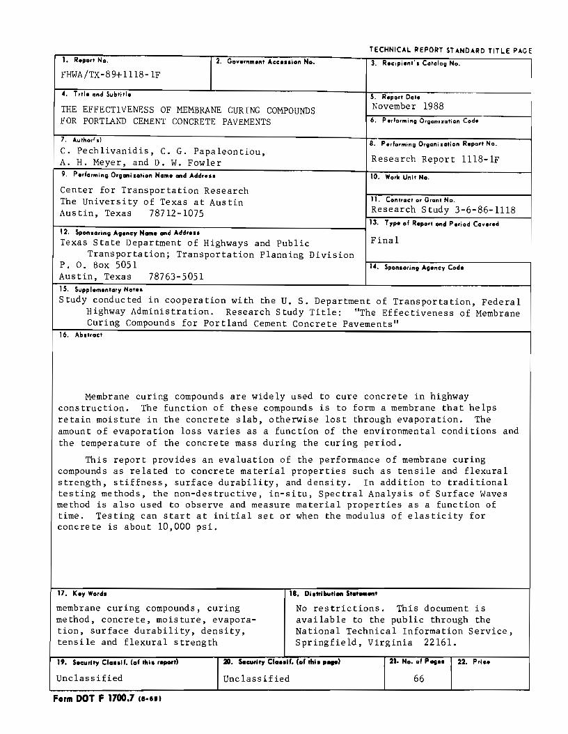
At each of these sites, after consultation with the District Engineer and the contractor, two pavement sections were set aside to be tested (except in site #6, in El Paso, where only one section was tested due to scheduling difficulties). These sections were textured mechanically by the contractor with burlap or Astrograss® drag and transverse tining as shown in Fig 3.2. On site #6 the transverse tining was done by hand as shown in Fig 3.3. The curing treatment was applied manually by the research crew.

The test sections were divided into panels having ap­proximate dimensions of 5 feet x 12 feet. Most of the panels

Regions Characteristics

V Dry, Freeze-Thaw II Wet. Freeze-Thaw I Wet, No Freeze

IV Dry, No Freeze

• Location of Experimental Site

Fig 3.1. Location of the experimental sites in the climatic regions of Texas.

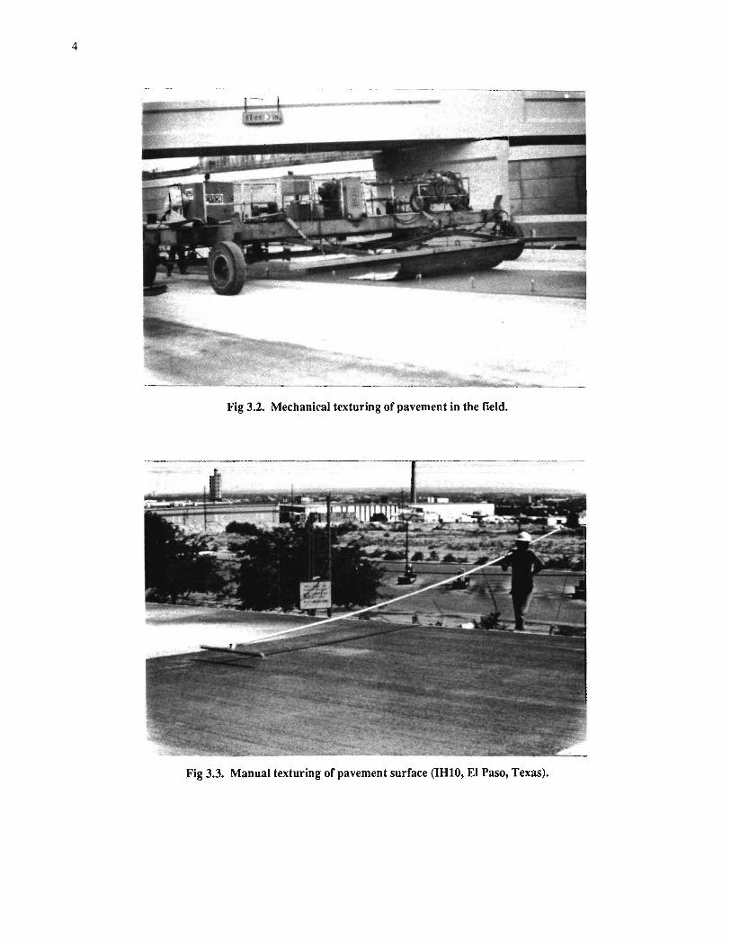
were sprayed with a membrane curing compound, while some were covered with polyethylene sheet, or left com­pletely untreated. Three coverage rates were used for the curing compound: 150, 180, and 200 square feet/gallon in three of the four field test sites (Districts 2, 5, and 12). In the fourth test site (District 24) an additional rate of 250 square feet/gallon was also used on one panel. An "airless" type, electric-driven spraying gun was employed for this opera­tion. A schematic of a typical panel layout is shown in Figs 3.4 and 3.5. Note that some curing treatments are repeated in order to provide a repetition of results for statistical pur­poses.

Three kinds of specimens were obtained in the field: 4-inch cores, 6-inch x 12-inch cylinders, and 6-inch x 21-inch beams. The beams and the cylinders were cast by the

research crew using concrete from the same batch that was used for the test

TABLE 3.1. PROJECT 1118 FIELD TESTING SCHEDULE panels on the pavement and were tex-

Test Site, Contractor Location District

#1 Tulia, Tx 5 #2 Tulia, Tx 5 #3 Ft. Worth, Tx 2 #4 Houston, Tx 12 #5 Houston, Tx 12 #6 El Paso, Tx 24

Placing Coring Date Date

7 {23/87 7{30/87 7 {24/87 7 !31/87 1{29/88 2/4/88 6/23/88 6/30/88 6{24/88 7/1/88 7{22/88 7{29/88

Environmental Zone

v v II I

v

3

tured by an Astrograss® drag and trans­verse tine grooving (Fig 3.6). The grooves were on the average 1/16 inch deep with 3/4-inch center-to-center spacing. The specimens were allowed to cure for seven days in the field under the same conditions as the pavement and they were then transported to the labora­tory for testing. At every test site in the

4

Fig 3.2. Mechanical texturing of pavement in the field.

Fig 3.3. Manual texturing of pavement surface (IHlO, El Paso, Texas).

Sta 344+30 -.-180 sq tvgal

Applied by the Contractor

No Curing ("Dry")

Polyethylene Sheet

6@ 5 ft

150 sq fVgal

200 sq fVgal

180 sq fVgal

Sta 344+00 -'-

1- 10ft ·I Fig 3.4. Section indicating the types or

curing applied to different panels (IH-45, Houston, Texas).

field the concrete was tested for slwnp, air content, and temperature at the time of placing.

Splitting Tensile Test

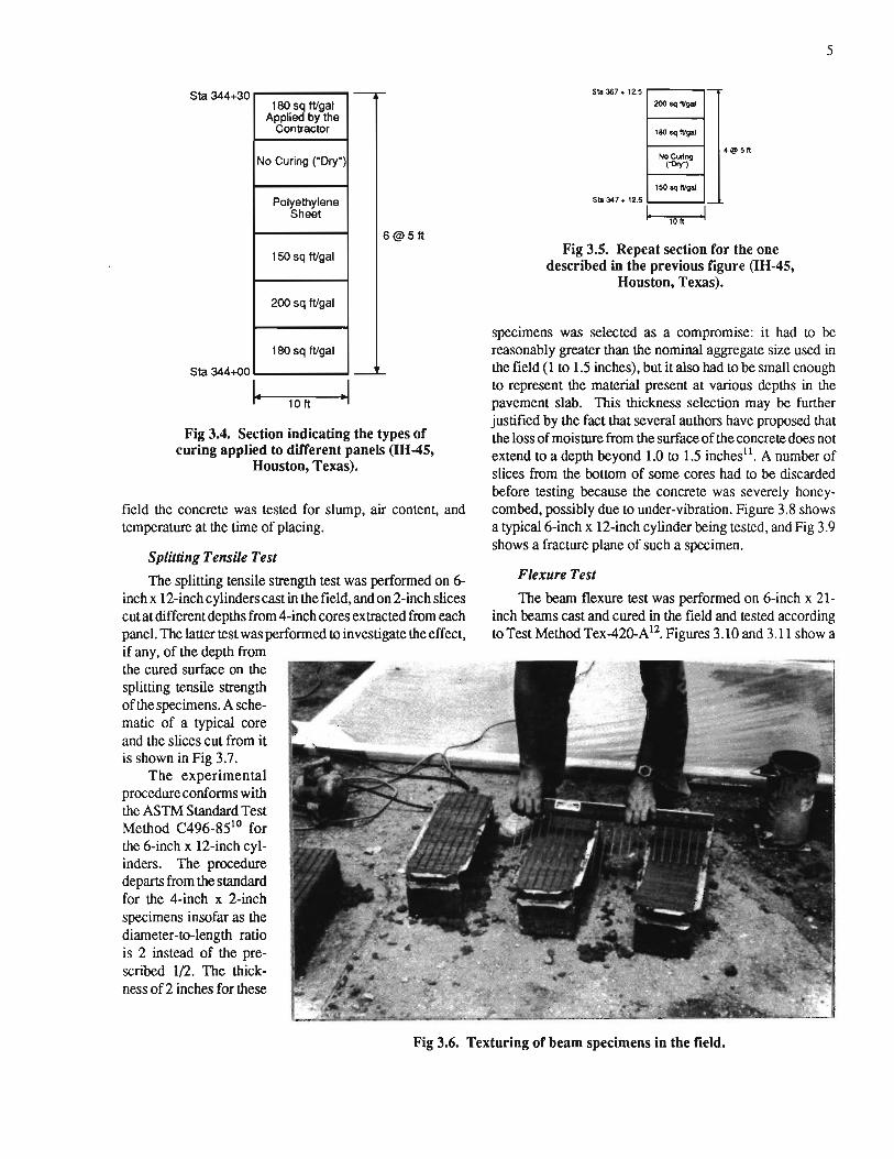
The splitting tensile strength test was perfonned on 6-inch x 12-inch cylinders cast in the field, and on 2-inch slices cut at different depths from 4-inch cores extracted from each panel. The laner test was perfonned to investigate the effect, if any, of the depth from the cured surface on the splitting tensile strength of the specimens. Asche­matic of a typical core and the slices cut from it is shown in Fig 3.7.

The experimental procedure confonns with the ASTM Standard Test Method C496-85 10 for the 6-inch x 12-inch cyl­inders. The procedure departs from the standard for the 4-inch x 2-inch specimens insofar as the diameter-to-length ratio is 2 instead of the pre­scribed 1/2. The thick­ness of2 inches for these

Sta 367 • 12.5 ,-200 oq 11/gal

180 oq 11/gal

NoCu1ng ("1l!y")

150 oq 11/gal

Sta347o12.5

I. 10ft

Fig 3.5. Repeat section for the one described in the previous figure (IH-45,

Houston, Texas).

5

specimens was selected as a compromise: it had to be reasonably greater than the nominal aggregate size used in the field (1 to 1.5 inches), but it also had to be small enough to represent the material present at various depths in the pavement slab. This thickness selection may be further justified by the fact that several authors have proposed that the loss of moisture from the surface of the concrete does not extend to a depth beyond 1.0 to 1.5 inches11

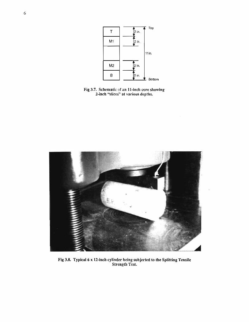
• A number of slices from the bottom of some cores had to be discarded before testing because the concrete was severely honey­combed, possibly due to under-vibration. Figure 3.8 shows a typical6-inch x 12-inch cylinder being tested, and Fig 3.9 shows a fracture plane of such a specimen.

Flexure Test

The beam flexure test was perfonned on 6-inch x 21-inch beams cast and cured in the field and tested according to Test Method Tex-420-A12

• Figures 3.10 and 3.11 show a

Fig 3.6. Texturing or beam specimens in the field.

6

Top T 2 in.

M1 2 in.

1 lin.

M2 ~in.

B 2 in. Bottom

Fig 3.7. Schematic of an 11-inch core showing 2-inch ''slices" at various depths.

Fig 3.8. Typical 6 x 12-inch cylinder being subjected to the Splitting Tensile Strength Test.

Fig 3.9. Typical fracture plane of a specimen tested as shown in the previous figure.

Fig 3.10. Typical flexure beam being tested in the Reinhard Beam Tester.

7

8

typical beam being tested, and a fracture planeofsuchaspecimen.

Surface Durability Test

The testing proce­dure used to detennine the variation in surface durability, between dif­ferently cured speci­mens, is based on the ASTM Standard Test Method C418-81 13

• In the standard ASTM method, the specimen surface is initially as­sumed flat and the vol­ume of the abraded cavi­ties is measured using a oil-based clay. Because the initial surface in this experiment was tex­tured, the use of clay was not considered practical. Instead, the specimens were weighed before and after the test to detennine the weight loss caused by the sandblasting.

The specimens used were 4-inch cores ob­tained in the field similar to the ones used for the splitting tensile test. The top surface of each core was sandblasted at eight different locations. Fig­ure 3.12 shows the appa­ratus used in the test

Core Density Test

A concrete density test was perfonned on 2-inch slices taken from the top and the bottom of cores obtained from test panels in the field to de­tennine if various curing methods have any effect

Fig 3.11. Typical fracture plane of a specimen tested as shown in the previous figure.

.r·----=----.,

Fig 3.12. The sandblasting cabinet used for the Sandblasting Abrasion Test.

on the density of the pavement material. The test was perfonned according to the ASTM Standard Test Method C642-8214

.

Spectral Analysis of Surface Waves (SASW)

The SASW method is a non-destructive, seismic test procedure primarily used in the field of soil mechanics for in-situ measurements of soil characteristics such as con-

strained and shear moduli and layer depth. In the study of pavements it has also found uses in the determination of structural integrity and stiffness profiling.

Its application in fresh concrete has been rather limited. One of the general objectives of the present study is to determine if the advantage of non-destructiveness offered by SASW can be utilized for testing concrete at its early stages when such a requirement is absolute. Since most other concrete testing procedures are either destructive or can only be performed on hardened concrete, the advantage of using SASW is obvious. Additional SASW advantages stem from the fact that all testing is performed in-situ and essentially instantaneous. Therefore, the material tested is not only of considerably larger volume than that of laboratory speci­mens - and thus is more representative - but it is also the actual material that will be required to perform during the lifetime of the pavement

Finally, there is an additional advantage to SASW, as compared to traditional testing methods, which is especially useful in the case of concrete. This is the fact that SASW allows the researcher to trace the change of material proper­ties during the curing period on an almost continuous basis by taking measurements at close time intervals beginning shortly after placing. A particular objective of this study was to utilize SASW as an alternate method in evaluating the effect of the application rate of membrane curing com­pounds (MCCs) on the modulus of elasticity, and therefore the strength, of freshly placed concrete. It was envisioned that the SASW would not only measure such properties at a given time, but also measure their rate of change in time, and compare the different rates of change resulting from different MCC application rates.

The general principle in all seismic test methods is that the response of a body of material to induced stress waves can yield useful information about its properties. An expla­nation of the theoretical basis of seismic testing in general, and SASW in particular, is quite involved and is beyond the scope of this report An excellent discussion with some emphasis on concrete applications is a report on several factors affecting SASW and is found in Reference 15.

SASW testing was performed at the test site in District 24. Measurements were taken during a period of six days, on five panels, each cured differently.

Figures 3.13 and 3.14 show close-up views of the instruments used. Figures 3.15 and 3.16 show the arrange­ment of all sources and receivers in a test section. All signals from these instruments were transmitted to a Dynamic Signal Analyzer that performed a partial analysis of the data on-site as it was being received. The data was then saved on floppy disks for further analysis.

P-Wave Test

In addition to the SASW test, the P-wave test was performed on all panels discussed in the preceding section and also on cores taken from each of those panels.

9

The difference between the SASW and the P-wave tests is that the former uses Rayleigh surface waves while the latter uses compressive body waves in the tested material. The objective of the P-wave test is to measure the time interval required for a compressive wave to travel the dis­tance between the wave source and the receiver. This, in tum, allows for the calculation of material properties such as Young's modulus. The formula used is:

E = p v 2 [(l+J.I.) (l-2J.1.)] I (1-J.I.) p

These are based on small strains and represent initial tangent modulus. where

E = modulus of elasticity, p = mass density,

v = compression wave velocity, and p

ll = Poisson's ratio (0.25).

Figure 3.17 shows the configuration for the P-wave test performed on cores.

Modulus of EhJsticity Test

Six cores from the test site in District 24 where the SASW testing was performed were also tested to measure their modulus of elasticity for comparison purposes with the values derived from SASW. The cores were tested accord­ing to the ASTM Standard Test Method C469-8316

•

The dimensions of the cores were 3.7 inches x 7.5 inches. After testing for the modulus of elasticity the cores were tested in compression according to the ASTM Standard Test Method C39-8617.

LABORATORY TESTING A limited amount of testing was conducted during the

laboratory phase of the project to complement the field phase. For every batch of concrete mixed in the laboratory the following tests were performed: Slump (ASTM Cl43-7818), air content (ASTM C231-8219), and unit weight (ASTM C29-78~. In addition, the concrete temperature was measured at the time of placing. The beams and cylinders were prepared according to Tex-420-A21 , and ASTM C496-8522, respectively. The curing was performed as described at the beginning of this chapter.

Splitting Tensile Test

The splitting tensile test was used to investigate the effect, if any, of different curing methods on the indirect tensile strength of 6 x 12-inch cylindrical specimens.

The test was performed according to the ASTM Stan­dard Test Method C496-8523•

Flexure Test

The beam flexure test was performed to investigate the effect, if any, of different curing methods on the flexural

10

strength of 6 x 21-inch concrete beams. The test specifica­tion followed was TEX-420-A2A.

Spectral Analysis of Surface Waves (SASW)

The feasibility of applying the SASW method to fresh concrete was tested in the laboratory before it was applied in

the field. For testing a concrete beam was made, measuring 12 feet x 11 inches x 4 inches Two sources and three receivers were placed as shown in Fig 3.18. Measurements were taken in the interval between 2 and 13 hours after the concrete was mixed.

Fig 3.13. Close-up view of the source and receivers used in the SASW test.

Fig 3.14. Close-up view of the receivers used in the SASW test. The spacing between the first and the second receivers from the left is one foot, and the spacing

between the second and the third receivers is 0.5 foot.

5

2 I

3@5ft I • 1

I

I

'

Panel 1: No Curing ("Dry") Panel 2: 150 sq tvgal Panel 3: 250 sq tvgal Panel 4 · 180 sq fVgal Panel 5: Cured by the Contractor

at 180 sq fVgal Panel 6: Polyethylene Sheet Panel 7: 250 sq tvgal

4 . I . • . •

3

:~ Receivers

• Source

3@ 8 It 7 in.

7

6

Fig 3.15. SASW panel configuration. Only panels 1, 2, 3, 4, and 7 were tested (IH-10, El Paso, Texas).

r-

18 in.

~ • +---Receiver #3 12 in.

Sit r-- · +----Receiver #2 6 in. ~ 1 +---Receiver #1 6 in .

.......__ • +--Source

.... I•

8 It 7 in. •I

Fig 3.16. Detail or a SASW test panel showing the source-receiver configuration. The slab has a thickness or 11 inches (IH-10, El Paso, Texas).

11

12

~~~--------d--------~·1

1+--- Metal Plate

Circuit Breaker Osciloscope

Receiver

Fig 3.17. Configuration for a P-Wave test on a core. Drawing not to scale.

6 in. 6 in. 6 in. 6 in.

1~ t t ,~ •1 I Source 1 Receiver

Fig 3.18. SASW experimental setup on a 12-foot beam showing source and receiver spacing. The beam has a width of four inches.

(Drawing not to scale.)

CHAPTER 4. EXPERIMENTAL DESIGN

FORMULATION OF THE EXPERIMENT This chapter describes the field experiment that was

conducted in order to investigate the effect of various meth­ods of curing of concrete pavements on concrete strength and durability.

Whendesigninganexperimentitisimperativetorecog­nize frrst those factors that may influence the variable under investigation. This variable is called the dependent variable where as the other factors are called the independent vari­ables. In the particular experiment the following variables have been identified.

dependent variables: concrete strength • flexural strength • indirect tensile strength • compressive strength

concrete durability independent variables: method of curing

contractor concrete mix design humidity ambient temperature depth at which strength is ob­tained

The next step is to set the limits within which the results will apply. These limits are called the inference space. It is preferable the results of this experimentation to apply to all contractors and concrete strengths and at any climatic con­ditions. In this case the experiment should be conducted in a way to include a sufficiently large random sample of contractors evenly dispersed within the state so that all climatic regions are represented. The contractor will then become the experimental unit that will be used to receive the application of each of the selected independent variables and be representative of the inference space. In simpler terms, all the combinations of variables will be repeated for each contractor, and thus the whole experiment will be repeated for each contractor.

Next, a final selection of the variables and their levels is made, taking into consideration the desired inference space, and the limitations imposed by construction practices as well as time and cost limitations. After a careful selection, the following variables were chosen to be included in the study:

(1) contractor (2) section of pavement for each contractor (3) method of curing ( 4) depth at which the strength is obtained (5) number of cores (6) rate of evaporation

These variables will be discussed in detail in subsequent sections.

The final step is the selection of the number oflevels for

13

each variable. Levels are the different values within the same variable, e.g., the different methods of curing in the method of curing variable, or the number of contractors in the contractor variable, that are under investigation. The selection of the number of levels is a very important aspect in the design, especially in experiments as large as this one. A slight increase in the number of levels may add a consid­erable amount of effort in running the experiment without gaining much more information from the additional data. The statistical modeling can be used to optimize the levels that will provide the desirable information at the least effort and cost. This may be demonstrated by the example. If each of the six factors is assumed to have two levels, the total number of combinations becomes 26 = 64. This means that a total of 64 cores are needed to conduct the experiment. If the decision is made to obtain three cores instead of two, then the total number of cores needed becomes 25 x 3 = 96 or 33 percent more. The same principle applies to the number of contractors needed. Contractors are, like cores, a random variable meaning that it can have unlimited number of levels, as compared to the method of curing which is a fixed variable. In most cases the selection of the number of levels for the random variables depends on the type of experiment (factorial, nested, etc.) which governs the tests for signifi­cance (called F test) of the main factors and interactions. The number of levels are selected so that the variance of the error term which is the denominator in the F has at least 4 to 5 degrees of freedom. At this level of de~ of freedom the F value obtained from the F distribution table becomes low enough to detect statistical differences among the tested factors. At higher degrees of freedom the F gets even lower but the difference does not justify th~u~xpense of getting more levels for each factor. Based on the above, it was decided to select a total of six contractors with the reservation to evaluate and possibly adjust this number as data was collected.

CLASSIFICATION OF VARIABLES This section describes in detail the selected variables

and their levels used in the experiment Field Testing

Contractor (CONTR). This is a broad variable which necessarily includes several aspects of pavement construc­tion that are difficult to treat separately. These aspects include:

* F test = MS types/MS error MS =

df= Fa! = v ue

mean square = sum of square deviations around the mean/df degrees of freedom the critical value ofF for a certain probability level and df.

14

(1) The Inherent VariabiUty in Quality Control Be· tween Contractors. Some contractors are more experienced or motivated than others and therefore are able to avoid problems such as applying MCCs too late or too early, failing to mix MCCs continuously during the spraying operation, etc. These poor construction practices are diffi­cult to detect and at times are left uncorrected. It is therefore difficult to estimate the amount of damage they may cause to the overall pavement quality.

(2) Mix Designs. The size and kind of aggregate used, the type of cement, and the quality control at the hatching plant are factors that are independent from the curing prac­tices and at the same time of great importance to the quality of the final product.

(3) Methods of Construction. Three methods of con­struction were encountered during the field phase of this project: one-layered and two-layered slip-forming and manually placed concrete.

The scope of this project does not allow the considera­tion of all of the above mentioned factors separate! y. Instead it was decided to "lump" them together and, if the analysis showed the variable contractor to be a significant source of variability, to recommend a further, more detailed study. The variable CONTR has six levels, equal to the number of sites were the test was performed.

Section (SECI'). On test sites where two sections were tested, the second section contained test slabs which were treated as the corresponding slabs at the first section. The variable SECT has one or two levels depending on the number of sections per site.

Curing Method (RATE). The most obvious and impor­tant variable to be considered when evaluating the effective­ness of MCCs is their rate of application. Several rates are suggested in the literature or specified by various agencies throughout the United States: 150, 180, and 200 square feet/ gallon.

In order to gain an understanding of the extent of any benefit provided by the MCCs, some concrete panels were allowed to cure without applying any curing treatment at all ("DRY" panels).

An additional curing method which was employed was the use of a polyethylene sheet. ("POLY" panels). This method is occasionally used in pavement construction.

The variable RATE has five levels: EX, POLY, 150, 180,200,250

where EX is the rate applied by the contractor at an area

adjacent to the test section (specified at 180 square feet/ gallon),

POLY signifies that the test panel was covered with a polyethylene sheet,

150, 180,200 and 250 are the application rates, square feet/gallon

Position (POS). As discussed in Chapter 3, the degree to which the curing of the exposed surface affects the full

mass of the concrete is not believed to extend beyond 1 to 1.5 inches. This top layer also happens to be the most important part of the pavement in terms of durability. A poorly cured surface results in cracking, which in tum, can lead to a multitude of other problems. It was therefore decided to isolate and test this part of the pavement and to compare the effect of curing on the material near the surface and at other depths.

The variable POS has four levels: T,M1,M2,B

where T 2-inch slice off the top of the core M1 2-inch slice between 2 and 4 inches from the top, M2 2-inch slice between 2 and 4 inches from the

bottom, and B 2-inch slice off the bottom of the core. Core (CORE). The variable CORE has one to four

levels depending on the number of cores extracted from each slab in each section.

RateofEvaporation(EVAP). Thereexistfourenviron­mental zones in Texas in all of which concrete pavement construction takes place on a continuous basis. This fact dictates the need to determine the extent to which different environmental conditions affect the performance of MCCs. The environmental parameters that are considered impor­tant to the curing of concrete are: ambient temperature, relative humidity, and wind velocity. A fourth parameter closely related to these is the temperature of the concrete. All four parameters can be combined to yield the amount of moisture loss by evaporation from the concrete surface, expressed as the weight of water lost per unit area of the exposed surface per hour. Figure 4.1 shows a chart offered by the Portland Cement Association25 from which the evaporation rate of a concrete surface can be found by entering the values of the four parameters mentioned above.

While it is not specified, it is assumed that the moisture loss described in the PCA chart occurs from a concrete surface that is allowed to cure without the benefit of any curing treatment. This, of course, was not the case in this study presently, where MCCs or polyethylene sheet covers were used on most panels. Therefore the values estimated from the chart could only be useful as indications of the potential for moisture loss, against which the applied curing method must protect.

In addition, the PCA chart does not offer any guidance as to the time frame for which it is applicable. In other words, similar environmental and PCC conditions would not neces­sarily produce the same evaporation rates from the same slab at different times say, at one hour and at eight hours after placing.

In order to characterize a pavement for its potential to

lose moisture through evaporation, it would seem reason­able to use the calculated rate of moisture loss at the time the concrete stops bleeding and consider this as the stage were the evaporation potential is at its highest. This can be

justified since the stoichiometric quantity of water required for the hydration process is less than the actual quantity used in the mix design. (It would, therefore be reasonable to assume that the bleed water is unneeded excess and that as long as it covers the concrete surface the hydration process fully takes place regardless of outside climatologi· cal conditions.) As soon as the bleed water disap­pears, any further evaporation loss takes place at the expense of the hydration process while it is still at its early stages and largely incomplete. At a later time, even if conditions favor a higher evaporation rate, the available water for such a process to occur is less since it has already been used in hydration. Therefore, at such a time, any moisture loss by evaporation cannot be as extensive and may not be as critical as that which takes place earlier.

The above hypothesis was used in modeling the behavior of the slabs tested in this study. The rate of moisture loss used was calculated using climatological data that were measured or esti­mated at the time the bleeding stopped. This was also the time when the MCCs were sprayed onto the surface of the slabs.

There is no indication that there is a theoretical basis for the PCA chart. and some objections have been raised as to its validity for some combinations of environmental conditions26; nevertheless it is useful as a "rule of thumb" that allows the substi·

5 15 25

RelaUve Humidity 100 percent

Air "femperarure (°F)

15

35

1.0

tution of one "resultant" variable (rate of evapora­tion) for four "component" variables (ambient temperature, relative humidity, wind velocity, and concrete temperature). This greatly reduces the number of variables in the statistical model.

Fig 4.1. The effect of environmental conditions and of tbe concrete temperature on moisture evaporation from fresh

concrete (Ref 25).

Specimen (SPEC). The variable SPEC refers to the 6-inch x 21-inch beams or to the 6·inch x 12-inch cylinders prepared at the test sites. It has one to four levels depending on the number of specimens prepared for each MCC application rate.

Laboratory Testing

Ambient Temperature. This variable represents the temperature ranges in which the beams and cylinders cast in the laboratory were cured. It has two levels:

where HandM

His 75 to l00°F, and M is 55 to 75°F.

PCC Temperature. This variable represents the tem­perature of the concrete at the time of placing. It has three levels:

H, M,andL where

H is 75 to 100°F, M is 55 to 75°F, and

L is less than 55°F. Ambient Relative Humidity. This variable represents

the relative humidity during the curing time of the speci­mens. It has two levels, H, and M where

His 70 to 100 percent, and M is 40 to 70 percent

Application Rate. Three MCC application rates were used. These were 150, 180, and 200 square feet/gallon. In addition, one specimen from each batch was moist cured to provide a basis for normalizing the data.

STATISTICAL MODELING The objective of the experiment was to investigate what

effect different methods of curing have on concrete strength and durability. In addition, the effectiveness of each curing method as a function of the depth of the concrete in the slab was investigated.

It was intended that the results of the testing to be applicable to all climatic regions of Texas and to all contrac­tors, construction methods, and concrete strengths. This

16

defined the inference space of the experiment and guided the selection of variables and levels that needed to be considered to achieve credible results. An important element in the selection process was randomization. As it was explained in the previous section, conttactors are the inferential unit in this experiment. It was, therefore, important to make a selection of conttactors that would give each an equal chance of receiving each treatment and confounded variance. Confounded variance is a lumped variance that results from a combination of factors which are not controlled during the experiment Since these factors are not controlled their variance can not be separated and attributed to them. It is desirable then to run the experiment in a way to allow the uncontrolled factors an equal chance of affecting the results. In this experiment the climatic differences in the four regions in Texas are assumed to have an effect. For this reason the contractors were selected at random in the four environ­mental zones of the state.

One very important aspect introduced in this experi­mental model is blocking. Blocks are experimental units that contain a complete set of treatment combinations. As a result there is only one restriction on randomization because the treatments in each block are carried out separately within each block. In this experiment conttactors are the blocks. All treatment combinations (SECT, RATE, CORE) are carried out for each contractor and the whole experimental procedure is performed before proceeding with an other contractor. The conttactors then, which are random repeats, become the inferential units. Inferential units are random elements that provide the basis for inference and, in general, are not of interest per se. In other words, when blocks are truly random one is not interested in differences among them and interactions of blocks with the treatments within the blocks should not be significant. What is of interest is the main factors such as RATE or POS, or their inter-

A second and most important feature of blocking is that it can remove a large variance from the error term and thus facilitate easier detection of treatment differences between important factors such as RATE and POS. If a block design experiment is analyzed like a completely randomized design then the portion of the variance that could have been attrib­uted to blocks would go into the error term with the result of· increasing the error variance. The net effect would then be a more difficult detection of treatment differences. If, on the other hand, blocking does not remove any variance from the error, then pooling of variances can be performed resulting in an error term without any blocking effects. This shows that blocking is always helpful because it can result in easier rejections and that it is never harmful because variances can be pooled back to the error term if required.

For every contractor except #6, two random repeats of the experiment were performed. That is, five to seven methods of curing were repeated at two pavement segments.called sections. The experiment was designed to eliminate the possibility of losing the blocking effects if the contractors were found to be fixed treatments. This would mean that some unique factors are confounded within the variable CONTR such as those described in the beginning of this chapter. That could cause an inflated error term and could minimize the chance for detecting treatment differ­ences. If CONTR were found to be fixed the inferential units tests of significance would have to be the sections; the sections are true random blocks since they do not involve fixed variations but are only repeats of the concrete mix design and construction practices of the same contractor.

The experiment was designed as a nested factorial with blocking. The treatments and levels used are described in the following table:

No. or actions. When interactions of blocks Variable Treatment Designation Levels Designation

Random Contractor CONTR 6 Nl-N6 with treatments are significant then there is high probability that some­thing was fixed during the experiment and that contractors (blocks) were not random repeats. If, for example, the CONTR * POS interaction is signifi· cant then there is high certainty that

Random Fixed

Contractor Replication Curing Method

SECT RATE

2 Sl,S2 7 150,180,200

POLY, EX, DRY Test Core CORE 1-4 1-4 Random

Fixed Vertical Position of Core Slice POS 4 T,M1,M2,B

the combination of these two variables did not affect in the same way the strength of concrete in the various contractors. What might have happened is that one contractor might have under·vibrated the pavement at the bottom and this resulted in lower bottom strength. The above discussion shows the importance of blocking in an experiment in that it can detect peculiarities in the way the experiment was really performed and alert for violation in the assumptions used. Significant block-treatment interactions can be detected by comparing their mean squares. If these interactions are indeed signifi­cant then their mean squares are statistically different.

In a nested factorial experiment all the levels of a factor that is nested in another factor are different across the level of the other factor. In such an experiment, in addition to a nested factor, a factor or factors may have the same levels across other factors and be factorial to these factors as well. In this experiment the conttactor replication, (SECT), is nested within contractor, (CONTR), because all sections are different. On the other hand, the application method, (RATE), is the same across all the levels of CONTR and SECT and is therefore factorial to these factors. Likewise, cores, (CORE), are nested in conttactor- contractor replica-

17

CONTR 1 2 3 4 5 6

1sEcD SECT SECT SECT SECT SECT

3 4 5 6 7 8 9 10 11 RATE CORE POS

T

1 M1 M2

EX B T M1

2

=±EE M1

1 M2 B

POLY T M1 M2

2 B T

Fig 4.2. Schematic or a nested factorial experiment.

tion- application method, (CONTR- SEC-RATE). Finally, position, (POS), is factorial to contractor- contractor repli­cation- application method-core, (CONTR- SECT-RATE - CORE). The set-up of an experiment such as the one discussed but with only two curing method levels is shown schematically in Fig 4.2. Note the sequential numbering of SECT and CORE levels to represent the nesting, and the repeated munbering of POS levels to show their factorial nature.

The experimental model can be written as a linear model in the form of an equation that predicts the response variable strength (STRG) as a function of the main variables, nested factors, and interactions. This equation is of the form

STRG .... , __ = J..L + CONTR. + SECT(.)" + li( .. ) + RA TEk + ljLUJUl 1 1 ~ IJ

where

CONTR *RA TEik + SECf*RA TE(i)jk +

CORE(ijk)l + ro(ijkl) + POSm + CONTR *POS. + SECT*POS(·)· +

1m IJm

RATE*POSkm + CONTR*RATE*POS.k +

1 m SECT*RATE*POS(i)jkm +

CORE*POS(ijk)lm + E(ijklm)n

STRGi'klmn = strength of a specimen n obtained from J contractor i, section j, treated with curing

method k, occupying position m in core 1; J..L = overall mean;

CONTR. = effect of the contractor i; I

SECT(i)j =effect of contrac~r replication j nested within contractor 1;

li(i") = randomization restriction error on contractor J 1' . rep 1cauons;

RA TEk = effect of the curing method k;

CONTR *RA TEik = effect of the interaction of contractor i with curing method k;

SECT*RA TE(i)"k = effect of the interaction of contrator ~ replication j with curing method k nested

within contractor i;

CORE(i"k)I = effect of core I nested within contractor i, J section j, and curing method k;

ro(ijkl) =randomization restriction error on cores;

18

POSm ==effect of position m;

CON1R*POS. ==effect of interaction of position m with un .

contractor 1;

SECf*POScr ==effect of interaction of position m with 1 ~m section j, nested within contractor i;

RA TE*POSkm == effect of interaction of position m with curing method k;

CON1R *RA TE*POSikm ==effect of interaction of position m With curing method k, and contractor i;

SECT*RA TE*POS Oikm == effect of interaction of position m

1\1/lth curing method k and section j,

nested within contractor i;

CORE*POS C .k)lm == effect of interaction of position m with 1J core 1, nested within curing method k,

section j, and contractor i; and

ECklm) == random error of the nth specimen of contractor, 1J n section j, curing method k, core 1, and

position m.

Contractors were selected at random in different envi­ronmental regions in Texas in order to broaden the inference space of the experiment so that the results would be appli­cable to any contractor at any environment The variable CON1R includes a known variance partly resulting from the different contractors examined in the study and a con­founded variance that may be a result of different concrete mix designs at the contractor level or other factors as discussed at the beginning of this chapter. Therefore it should be emphasized that inferences on this variable should be made cautiously in light of the fact that a wide variety of unmeasured effects are built into the variable.

The error d(i .) is the first restriction error on randomiza­tion which reco~nizes the peculiarity that randomization occurs over each section separately as soon as a section is considered and not over the whole experiment as would the case be in a completely randomized design. This restriction prevents any inference to be made on the variable SECT which is not of interest by itself. A second restriction on randomization, w (i"kl)' occurs within each core because test­ing of each core ta6k place after it was obtained and not over the whole experiment. This prevents any inference to be made on the variable CORE, but again, this variable is not of any interest in the evaluation of MCC treatments and there­fore no information is lost These two restrictions were not placed by design but were a physical result of the way the experiment was performed. However, the limitations they pose should be recognized as part of the analysis.

The algorithm of the expected mean square errors (EMS) for each source of variation is shown in Table 4.1. For a fixed component of variance the F notation is used, and for a random component the notation s2 is used. The arrows show the tests for significance (F-test) for each source of variance. The CON1R mean square is the main inferential unit and is used to make all the important tests which are RATE, POS, and RATE*POS. The SECT variable is used as a "secondary" inferential unit and makes all the tests of the interactions between CON1R and the important factors: CONTR*RATE, CONTR*POS, and CON1R *RA TE*POS.

It is interesting to note that CORE mean square makes the less important tests: SECT*RA TE, SECT*RA TE*POS. This means that it is not necessary to obtain a large number of cores for each treatment combination of CON1R, SECT, :md RATE. In fact., since each treatment combination in­volves at least 6 contractors x 2 sections x 6 curing methods == 72 cores, it is not necessary to obtain more than one core per treatment combination. An examination of the F­distribution table shows that at a level of 0.05 and for six degrees of freedom for the treatment under consideration the F 5 72

value needed to reject equality is 2.36. The correspond­ing F 5 144 value for the case of two cores per treatment combination is 2.28. This suggests that the added expense of obtaining the additional specimens is not justifiable by a reduction of only 0.08 in the F-value. For this reason it was decided, after a preliminary analysis such as the one dis­cussed above, to limit the number of cores per treatment combination from the three or four that were being taken from sites # 1, #2, and #3 to only one from the remaining sites.

The maximum number of specimens obtainable if only one core were taken per treatment combination would equal 336. In actuality, the total number of specimens obtained was somewhat less because some of the specimens had to be discarded because they were severely honeycombed or damaged during transportation.

The importance of an experimental design that blends the engineering needs and limitations with the mathematical aspects of statistics can not be overemphasized. The statis­tical considerations become increasingly important in ex­periments with many factors and with construction se­quences that impose restrictions to the models and derive the methods for analyzing the data. The experiment designed for this study has provided guidance for the practical and systematic application of the theory in the field. It has helped with selecting the optimum number of levels of contractors and cores for the random factors that would provide reliable information at a reasonable cost. It has helped with detecting errors introduced into the model that violate the initial assumptions.

DF

2 3 0

4 8

12 30 0

1 2 3 4 8

12 30 0

19

TABLE 4.1. DERIVATION OF THE EXPECTED MEAN SQUARE (EMS) ALGORITHM

Fixity

RRFRFR

1 j k I m n

1 2 5 2 2 1 1 1 5 2 2 1 1 1 5 2 2 1

3 2 0 2 2 1 2 0 2 2

1 0 2 2 1 1 1 1 2 1

1 1 1 1 2 1

3 2 5 2 0 1 125201 1 1 5 2 0 1 3 2 0 2 0 1

2 0 2 0 1 1 0 2 0 1 1 0 1 1 1 1

Source

CONTRj SECf(i)j 8(ij)

Expected Mean Squares

a2 + 2o2coRE + zao2a + 20o2sEcr + 40o2coNTR a2 + 2o2coRE + 20o2a + 20o2sEcr Jlf a2 + 2o2coRE + 20o2a

RATEk a2 + 2o2cORE + 4o2sECT*RATE + 8o2cONTR*RATE + 24<1>(RATE) CONTR*RATEik a2 +2o2cORE +40'2SECT*RATE + 8o2cONTR*RATE Jlf SECT*RATE(i)jk a2 + 2o2cORE + 4o2SECT*RATE Jlf CORE(ijk)l a2 + 2o2cORE ;tf O>(ijkl) a2 + 2o2coRE

POSm a2 + a2coRE*POS + 10o2sECT*POS + 20o2coNTR*POS + 60<1>(RATE) CONTR*POSim a2 + a2cORE*POS + 10o2SECT*POS + 20o2CONTR*POSJif SECT*POS(i)jm a2 + a2cORE*POS + 1 Oo2SECT*POS Jlf RATE*POSkm \ a2 + a2coRE*POS + 20'2sECT*POS + 40'2coNTR*POS + 12<1>(RATE) CONTR*RATE*POSikm a2 + a2cORE*POS + 2o2sECT*POS + 40'2CONTR*POS Jlf SECT*RATE*POS(i)jkm a2 + a2cORE*POS + 2o2sECT*POS ;tf CORE*POS(ijk)lm a2 + a2cORE*POS Jlf E(ijklm)n 02 ;tf

CHAPTER 5. EXPERIMENTAL RESULTS

FIELD EXPERIMENT

Splitting Tensile Strength Test (Cores)

The analysis of the data obtained by the splitting tensile strength test on 2-inch slices of cores obtained in the field was done by constructing several statistical models which are variations of the general model described earlier, in Chapter 4. The reason for using more than one model was to take into account some particular characteristics of the data with models that emphasized those characteristics, or to conform with memory limitations of the computer systems used. The data used in the analysis are presented in Tables A.l to A.5 in Appendix A.

ModellA. This model is similar to the general model described earlier with the only exception being that one high order term, CORE* POS (RA1E SECT CON1R), was excluded because of memory limitations in the computer used for the analysis. It is assumed that no significant amountofinformation is lost from this exclusion because the interaction is of very high order.

In this model all classes of all variables are used and no attempt is made to transform the data in any way. Finally, the effects of environmental conditions are not taken into ac­count. The model is described in a concise form in Table B .1 in Appendix B.

Modell B. The motivation for this model was a prelimi­nary analysis of the data that indicated no statistical differ­ence in strength between the top and the bottom positions. This, along with field observations and examinations of retrieved specimens, prompted a concern that possibly lower top concrete strengths were being masked by low bottom concrete strengths that were due to factors other than curing, such as under-vibration or other construction practices. This would lead to the erroneous conclusion that the top and bottom strengths were the same. It was therefore decided to obtain and test two specimens from the middle of each core, a position which intuitively was considered to represent the highest concrete strength. This operation was only per­formed for contractors four, five, and six. Model lB repre­sents an analysis that considers only those contractors from which specimens from all four positions were taken.

From a statistical point of view the model is similar to model1A, the only difference being the number oflevels for the variablePOS. Table B .2 offers a summary description of this model. This and all subsequent tables presenting the results from the analysis of variance are divided into two parts. The top part of each table shows the variables used in each model, the nwnber of levels in each variable, and the values of each level. The bottom part shows the sources of variation resulting from the variables and their interactions; the degree of freedom for each source of variation; the F which is obtained by dividing the mean square (varianc~fgf the source in question by the mean square of the appropriate

20

error term; and the probability of making an error (type a) when rejecting the hypothesis that all levels within a particu­lar variable are equal. This probability is compared to an alpha level of 0.10 and significant differences are stated with a "yes."

Modell C. This model is complementary to modellB described above, in that it considers only the top and bottom levels of the variable POS over all the contractors. This was done in order to have a more balanced model in terms of treatment combinations than lA by having an equal number o~ POS levels _over all the contractors. This is the only difference of thiS model with model lA. Table B.3 summa­rizes the model and its results.

Model JD. Previous discussions have indicated the existence of a number of variables confounded within the variable CON1R, namely construction practices, concrete mix design, etc. All strength data were normalized in respect to the strength of the quality control specimens that are regularly prepared, cured, and tested by the Texas SDHPT at each jobsite. This way it was hoped that any variation introduced by the concrete mix design would be controlled, and that the detection of different strength levels for various curing methods would be easier. In all other respects this model is the same with modellA. A summary of the model and the results obtained are shown in Table B.4.

Model JE. In this model, the evaporation variable EV AP is introduced, while retaining the normalized values of the data. This is a second step after model 1 D in trying to identify variables that are confounded within CON1R, to explain some of the variation associated with it, and to show more clearly the effects of curing methods and position on strength. Table B.5 summarizes this model.

Models 2A, 2B, and 2C. These models are similar to models 1A, lB, and lC respectively, but in these cases the variable CORE is excluded from the analyses and the asso­ciated variances are lumped with the error terms. All previ­ous analyses indicated the non-significance of all interac­tions with CORE at a level of0.25. This allows for pooling of the respective variances. Here, pooling is useful because it increases the chance of detecting any significance due to the increased number of available degrees of freedom in the error terms which in turn result in lower critical F-values. Figure 5.1 shows the layout of these experimental models. Note the absence of the core variable, as compared to the models shown in Fig 4.2. Tables B.6, B.7, and B.8, contain s~mmary description of models 2A, 2B, and 2C respec­tively, as well as the statistical results obtained.

Discussion of Results. As indicated in the analysis of variance (Tables B 1-B8) none of the models have detected any significant differences in the important variables RA 1E, POS and their interaction RA1E *POS. This means that(1) none of the seven methods of curing evaluated in the experi­ment has resulted in higher or lower concrete strength; (2)

none of the strength locations (top, middle, or bottom of core) has resulted in higher or lower strength; (3) none of the seven curing methods has indicated any difference in the top, middle, or bottom strengths. The statistical results are also shown in a graphical form in Figs 5.2 to 5.4. The concrete strength data shown were normalized as a percent­age of the tensile strength of control specimens. This removed any variation introduced from the different mix designs and made the comparison more meaningful. It is important to note that at this point we are not interested in the level of strength, as this varies with the randomly selected contractors and the design used by each contractor. but in the relative comparison among the methods of curing, position, etc. All figures show in the vertical scale the dependent variable which is the tensile strength and in the horizontal scale the independent variables RATE, POS, and RA TE*POS. All graphs are approximately horizontal lines which verify the indifference of strength in the method of curing, the depth at which the strength was obtained, and the combination of the two. The non-significance of the RATE*POS interaction is very clearly shown in Fig 5.3 as the lines are almost parallel and difficult to distinguish.

All models have shown that the variable CONTR is highly significant This information is not of any interest in this experiment in engineering terms but it is extremely important from a statistical point of view. It shows that the way the experiment was designed (by having contractors as random blocks) haseffectivelyremoved a very large amount of variation from other variables making the detection of shmificant variables much easier. Of course, no significant v~ _,bles have been found but the detection would be far more difficult if the experiment was modeled otherwise.

The non-significance of RATE, POS and RATE*POS was true for both normalized and unnormalized data, as well as for the case where the eyaporation conditions were taken into account The finding that a heavier curing compound application rate does not imply significantly higher strengths, as would be intuitively expected, should not be considered extraordinary in view of the fact that other authors have reported higher evaporation rates7 from speci­mens cured with heavier rates. Somewhat peculiar was the fmding that specimens that were left completely uncured ("DRY") had strengths as high as those sprayed with com­pound. This fmding was true even when top core layers were compared with bottom layers which presumably cure under more favorable conditions. This could be the result of some unmeasured factor during the experiment or could very well mean that curing does not really affect concrete strength but some other concrete property. Another possibility could be that curing affects only the strength of a very thin top layer, and that the strength of the 2-inch top layer examined in the test had apparently masked the difference.

21

CONTR 1 2

SECT 1 2 3 4

RATE RATE RATE RATE POS 150 180 200 150 180 200 150 180 200 150 1801200

T

+= M1 M2 B I

Fig 5.1. Layout of experimental models 2A. 2B. and 2C.

140

120

.t::

g,1oo ~

(i5 80 ~ "li.i c: 60

t5ll ~ 0

40

20

0 DRY 200 180 EX 150 POLY

Application Method

Fig 5.2. Application rate vs. tensile strength normalized as a percentage of the tensile strength of the control specimens. Field cylinders. mean values.

Splitting Tensile Strength Test(Cylinders) and Flexure Test

The results of the splitting tensile strength test and flex­ure test performed on 6-inch x 12-inch cylinders and 6-inch x 21-inch beams are shown in Tables A.6 and A.7 in Appendix A.

The statistical model used to analyze the data in this experiment is a simplified version of model IA described earlier with the exception that there are only three classes of variables, namely CONTR, SECT, and RATE. Variable CONTR has six levels, equal to the number of contractors; SECT has two levels, equal to the number of experimental sections at each site; and RATE has four levels: DRY, 150, 180, and 200.

22

140

... .----- • 120

100 .c. a, c: Q) 80 ..._ (j)

~ "(i) 60 c: ~ ~ 0 40

20

0 T M1 M2 B

Position

Fig 5.3. Position vs. tensile strength normaUzed as a percentage or the tensile strength or the control

specimens. Field cyUnders, mean values.

140

120

.c. 100 a, c: ~ 80 (j)

~ --o-- pos .. r "(i) 60 ----- POS·B c: ---- POS- M1 ~ --o- POS = M2 ~ 0 40

20

DRY 200 180 EX 150 POLY

Application Method

Fig 5.4. Interaction or application rate and position vs. tensile strength normaUzed as a percentage or the

tensile strength or the control specimens. Field cylinders, mean values.

The statistical results of the tests on both cylinders and beams are presented in Tables B.9 to 8.12 in Appendix B. Figures 5.5 and 5.6 are plots of the mean normalized tensile and flexwal sttengths of the tested cylinders and beams respectively.

As can be seen from both the tables and the graphs the results are similar with those obtained from the tensile tests on the cores. First, a change in the MCC application rate does not result in a significant change in either flexwal or tensile strength even with normalized data. Second, there is a significant difference in flexwal and tensile strength from

140

120 • • • • .c.

~ 100

~ (j) 80 ~ '(i) c: 60 ~ ~ 0

40

20

0 DRY 200 180 150

Application Method

Fig 5.5. Application rate vs. tensile strength normalized as a percentage or the tensile strength or

the control specimens. Field beams, mean values.

180

160 • • -------. .. .c. 140 a, c: 120 ~ (j) c;; 100 ..._ ::I >< 80 Q)

u:: ~ 60 0

40

20

0 DRY 200 180 150

Application Method

Fig 5.6. Application rate vs. flexural strength normalized as a percentage or the flexural strength or

the control specimens. Field beams, mean values.

contractor to contractor. This finding is again of no signifi-cant engineering importance as strength varies by mix de-sign, but it points out the importance of the statistical model.

Surface Durability Test

The results of the surface durability test performed on surfaces of cores obtained from sites four, five, and six are shown in Table A.8. They are are also shown in graphical form in Fig 5.7.

The statistical model used for analyzing the results is a simplified version of the nested factorial model used to analyze the results of the splitting tensile test results for the cores, as described earlier. Table B.13 shows that the rate of MCC application does not significantly affect the surface durability as measured by the sandblast test

en E ca .... .9 1/) 1/) 0

....J -..c:: Ol

~

5

4

3

2

DRY 250 200 180 150 EX POLY

Application Method

Fig 5.7. Surface durability (weight loss) vs. application method for sites #4, #5, and #6.

Core Density Test

The results of the core density test that was performed on cores obtained at sites one and two are shown in Table A.9.

The statistical model used for the statistical analysis of the data is the same with model1A which was used for the split tensile test on the core slices and was described previ­ously. As can be seen from Table B.14 and Figs 5.8 and 5.9, concrete density is not significantly affected by either the MCC application rate or by the position of the slice in the core from which it was taken.

Modulus of Elasticity Test and P-Wave Test

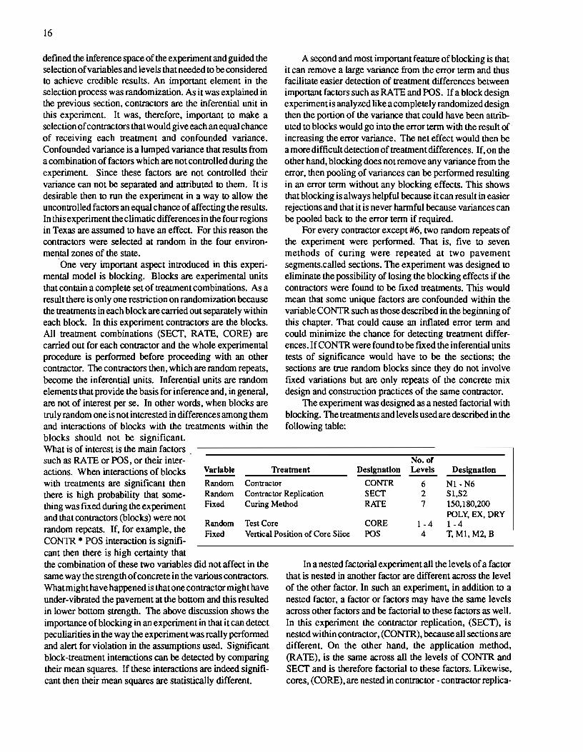
The results of the modulus of elasticity test performed on six cores obtained from site number 6 in District 24 are shown individually in Figs 5.10 to 5.15. Figure 5.16 shows

23

200

175

= ::I 150 ~ • • • • • 1/) ..0 ;:::.. 125 >-

:t:::: 1/)

100 c::

~ Q) 75 -~ CJ c:: 50 0 ()

25

0 200 180 150 EX POLY

Application Method

Fig 5.8. Concrete density vs. application method from field cores obtained from sites #1 and #2.

all readings together in one graph for comparison purposes. It appears from this graph that the modulus increases with increasing MCC coverage although there was no significant change in performance when this coverage varies between 250 and 180 square feet per gallon.

The six cores tested by the traditional ASTM method were also tested by the P-wave method to measure the modulus of elasticity as well. The results of this test are shown in Fig 5.17.

The differences between the two graphs appear in two levels; first, the results in the P-Wave graph are uniformly

200

175

= ::I 150 ~ • • ..0 ;:::..

125 >-:t:::: 1/) c:: 100 ~ Q)

75 -~ CJ c::

50 0 ()

25

0 lbp Bottom

Location

Fig 5.9. Concrete density at top and bottom 2-inch cores obtained from sites #1 and #2. (See Table 2.2.)

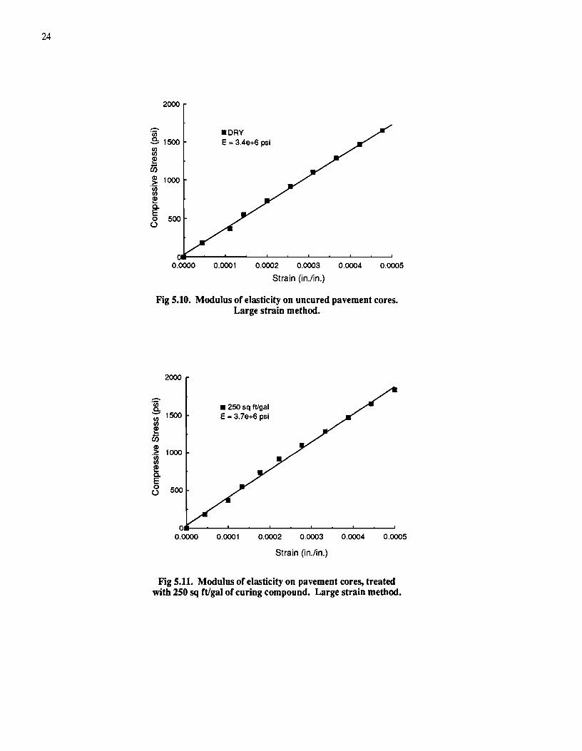
24

2000

-"iii

.e. 1500 :g ~

Ci5 ~ 1000 "jz ~ Q. E 0 500 (.)

0.0000

•DRY E = 3.4e+6 psi

0.0001 0.0002 0.0003 0.0004 0.0005

Strain (in./in.)

Fig 5.10. Modulus or elasticity on uncured pavement cores.

2000

i - 1500 :g ~

Ci5 ~ 1000 "jz ~ Q. E 8 500

Large strain method.

• 250 sq ft/gal E = 3. 7e+6 psi

0----~~--~--~------~--~~--~--~ 0.0000 0.0001 0.0002 0.0003 0.0004 0.0005

Strain (in./in.)

Fig 5.11. Modulus or elasticity on pavement cores, treated with 250 sq rt/gal or curing compound. Large strain method.

2000

~ - 1500 :a e

Ci5 .~ 1000 :a ! Q.

E 8 500

• 200 sq ftlgal E • 3.7e+6 psi

0----~~------~------L-----~----~ 0.0000 0.0001 0.0002 0.0003 0.0004 0.0005

Strain (in.lin.)

Fig 5.12. Modulus or elasticity from pavement cores.

2000

-'[ - 1500 !8 !

Ci5

-~ 1000

e ~ 0

(.) 500

Large strain method.

• 1 80 sq ftlgal E • 3.7e+6 psi

0------~------~------L-----~----~ 0.0000 0.0001 0.0002 0.0003 0.0004 0.0005

Strain (in.lin.)

Fig 5.13. Modulus or elasticity from pavement cores. Large strain method.

25

26

2000

-- • 150 sq tt/gal 'iii .& 1500 E = 3.8e+6 psi fJ) fJ)

~ U5 (D 1000 > 'jg I!! a.. E 500 0 ()

0.0000 0.0001 0.0002 0.0003 0.0004 0.0005

Strain (in./in.)

Fig 5.14. Application rate vs. tensile strength normalized as a percentage of the tensile strength of the control specimens.

--'iii .& m e

U5 ~ 'jg e a.. E 0 ()

Field cylinders, mean values.

2000

1500 • POLY E - 3.6e+6 psi

1000

500

0------~----~~----~----_. ____ __j

0.0000 0.0001 0.0002 0.0003 0.0004 0.0005

Strain (in./in.)

Fig 5.15. Modulus of elasticity on pavement cores, cured with polyethylene sheet. Large strain method.

higher than those of the previous graph by an average factor of 1.6. Second, the variation of values of the modulus between with each cov­erage rates is larger and no trend is apparent as was the case in the previous graph. This may be due to any one of several factors related to the novelty of the experiment and the limited number of available specimens that did not allow for familiarization with the testing proce­dures and any improvement upon them.

Spectral Analysis of Surface Waves (SASW)

The testing schedule for all SASW tests perfonned in District 24 over a period of six days is shown in Table C.l in Appendix C. Panel one, which was left completely uncured,

~

'[ II) :::l

:::l

'8 3.5e+6 :E II) -0)

c: :::l

~

27

All Values in Millions 3.8

DRY 250 200 180 150 POLY

Curing Method was used as the "control" panel. Because of equipment shortage one receiver set-up was left on this panel for the duration of the test and the second set-up had to be shuttled between all

Fig 5.16. Curing method vs. Young•s modulus at 28 days.

the other four panels. For this reason tests indicated in Table C.l in Appendix Cas #2 and #4 were not perfonned on panels two, three, four, and seven.

The results for each individual panel as plots of Young's modulus vs. time for wave­lengths, L, of 0.25, 0.50, and 0. 75 foot and a receiver spacing, R, of 1.00 foot are shown in Figs 5.18 to 5.22.

As a rule, shorter wavelengths represent the properties near the surface of the slab and longer wavelengths represent those at greater depth. Essentially, the measured stiffness is the average value over a depth equal to the wave­length, and can be considered under these condition to represent the stiffness at a depth half the wavelength. As can be seen from the graphs, for each panel, Young's modulus measured in test #8 is consistently lower near the surface, and higher near the bottom of the

8.5e+6

7.5e+6 -·c;; &

II)

-~ :::l

~ 4.5e+6

3.5e+6 DRY

Large strain method.

7.8

All Values in Millions

250 200 180 150 POLY

Curing Method

slab. The average value over all the slabs for a wavelength of0.25 foot ("top" of slab) is 4.3 x 106 psi. For a wavelength of 0.50 foot ("middle" of slab) the value is 4.5 x 106 psi,

Fig 5.17. Curing method vs. Young•s modulus at 28 days.

which is 4 percent higher, and for a wavelength of0.75 foot("bottom" of slab) the average valueis4.7 x lcf psi which is 9 percent higher than the first Nevertheless, a conclusion that the stiffness proftle of a slab can be accu­rately predicted should be considered cautiously because the scatter of the data appears to be within the overall experi­mental error.

A receiver spacing of 0.50 foot was also used, but part of the data thus obtained appears to have been severely affected by body wave reflections and must be excluded

P-Wave method (small strains).

from consideration for panels one, three, and seven. Figures 5.23 and 5.24 show the plots of Young's Modulus vs. Time for wavelengths of 0.~. 0.50, and 0.75 foot and receiver spacing of 0.50 foot for panels two and four. Figure 5.25 is an example of a plot such as the previous ones but which shows the effects of body wave reflections.

Tables C .2 and C.3 show moduli values averaged over all three wavelengths used for receiver spacings of 1.00 and

28

5.0

tO 4.0 0

X

"iii ..e, 3.0 (/) ::::l 5.0 ::::l

" 0 2.0 -o- L = 0.25 ft :::1!

(/) ---+--- L = 0.50 ft -01

----- L • 0. 75 ft c:

tO 0

4.0 X ~

::::l

~ 1.0 A= 1.00 ft

"iii ..e, (/) 3.0 ::::l ::::l

0.0 " 0 100 1000 10000

lime (min) :::1!

2.0 (/) -01

--o- L=0.25ft ---+--- L = 0.50 ft

c: ::::l ----- L = 0.75 ft

Fig 5.18. Young's modulus by the SASW method. ~ 1.0

Panel #1 (DRY). A =1.00 tt

tO 0

X ~

"iii ..e, (/) ::::l ::::l

" 0 :::1! (/) -01 c: ::::l

~

5.0

4.0

3.0

2.0

1.0

0 100

--a- L = 0.25 ft ---+--- L = 0.50 ft ----- L = 0.75 ft

1000

lime (min)

R = 1.00 ft

10000

Fig 5.19. Young's modulus by the SASW method. Panel #2 (150 sq ftlgal).

0

100 1000 10000

lime (min)

Fig 5.20. Young's modulus by the SASW method. Panel #3 (250 sq ft/gal).

5.0

tO 4.0 0

X ~

"iii ..e, 3.0 (/) ::::l :;

" 0 2.0 -o- L= 0.25 ft :::1!

(/) ---+--- L = 0.50 ft -~ ----- L = 0.75 ft ::::l

~ 1.0 R = 1.00 ft

0.0 100 1000 10000

lime (min)

Fig 5.21. Young's modulus by the SASW method. Panel #4 (180 sq ft/gal).

5.0

~ 4.0

>< -'8_ -3.0 0 ;::)

"5 -g ::i 2.0 0 ·rn c ;::)

~ 1.0

-o- L .. 0.25 ft --- L .. 0.50 ft --+- L .. 0.75 ft

R .. 1.00ft

0~-----~--~--~~-----~-----~~~~ 100 1000

lime (min) 10000

Fig 5.22. Y oungts modulus by the SASW method.

5.0

tO 0 4.0 .... ><

7i ..e, 0

3.0 ::I "5 -g ::i 2.0 .0

~ ::I

~ 1.0

0 100

Panel #7 (200 sq ft/gal).

--o- L • 0.25 ft --- L- 0.50 ft --- L-0.75ft

1000

lime (psi)

R- 0.50ft

10000

Fig 5.23. Young,s modulus by the SASW method. Panel #2 (150 sq ft/gal).

5.0

tO 0 4.0 >< -'iii ..e, 0

3.0 .2 ;::)

-g ::i 2.0 .0 0) c ;::)

~ 1.0

0 100

-D- L = 0.25 ft --- L = 0.50 ft --+- L= 0.75 ft

1000

lime (psi)

R = 0.50ft

29

10000

Fig 5.24. Youngts modulus by the SASW method.

5.0

~ 4.0

>< 'iii ..e, 3.0 0 .2 ;::)

-g ::i 2.0 0

-~ ;::)

~ 1.0

Panel #4 (180 sq ft/gal).

-o- L .. 0.25 ft --- L .. 0.50 ft -+- L=0.75ft

R • 0.50ft

0~-------------~~-----~-----------~ 100 1000

lime (min) 10000

Fig 5.25. Young's modulus by the SASW method. Panel (DRY).

30

0.50 feet, respectively. Figures 5.26 and 5.27 present the same infonnation schematically for comparison purposes. In both cases, and in particular in the case of the 1.00-foot receiver spacing where more data are available, a slight trend of increasing modulus values with increasing application rates can be detected. It is uncertain at this point. based on the amount of testing perfonned, whether this is a real trend, or nonnal data scatter.

These values should be compared with those obtained from the direct measurement of Yooog's modulus by the ASTM method, as described in the previous section.

Since the values obtained by the SASW method are six­day values and the others are 28-day values, it would appear that an adjustment in respect with time is necessary. It has been reported (Mindess, 1981)28 that the compressive strength of air-cured concrete at three days is about 65 percent of that of 28-day concrete. If this adjustment factor is used for the modulus of elasticity as well, the results by the SASW test would be about 90 percent higher than the mean of the values obtained by the ASTM test. This approach would clearly be unrealistic. Hence a theory is needed which would explain this discrepancy. A closer look at the SASW modulus of elasticity vs. time graphs shows that at six days the rate of change of the modulus in all panels had reached or was very close to reaching zero, indicating that the material had reached its stiffness limit. This may be related to the size of the hydrated cement grains which are smaller at an early age, or to the quality or quantity of bonding between cement grains which may change with age. Since both tests actually test the same material the long tenn moduli should be closer.

Under this assumption, it is reasonable to compare the six-day SASW results with the 28-day ASTM results directly. This comparison can be found in graphical fonn in Fig 5.28. The mean modulus value obtained by the ASTM method is 3.6 x 106 psi, and the mean value obtained by the SASW method is 4.5 x 106 psi which is about 24 percent higher.

A new set of modulus of elasticity readings that were obtained after the completion of this project (approximately four months after placement) has verified that the rate of change of the modulus is essentially minimal, and that the above assumption is a good approximation.

LABORATORY EXPERIMENT As mentioned before, the prevailing MCC coverage

rate is 180 square feet/gallon. Therefore, most tests were perfonned using this rate ooder various environmental conditions and concrete temperatures with the assumption that any trends in tensile or flexural strength dependent on such conditions would also apply for application rates other than 180 square feet/gallon.

Two tests were also perfonned using 200 and 150 square feet/gallon rates under medium ambient temperature,

6.0

<0 5.0 0

X

'iii 4.0 s 1/) ::J

3.0 "S "'0 0

::::E --<r- 150 sq fVgal .1/) 2.0 OJ --- 180 sq fVgal c:: -- 250 sq fVgal ::I

§:. 1.0 -o- DRY --e- 200 sq fVgal

R • 1.00 ft

0.0 100 1000 10000

Time (min)

Fig 5.26. Young•s modulus vs. time for a receiver spacing of 1.00 feet and averaged over wavelengths of

0.25, 0.50, and 0.75 feet.

5.0

<0 4.0 0

X

'iii s 3.0 1/) ::J "S "'0 150sq fVgal 0 2.0 ::::E 180sq fVgal 1/) ·a c:: ::I

1.0 §:. R .. 0.50ft

0 100 1000 10000

Time (min)

Fig 5.27. Average Young's modulus values for receiver spacing of 0.50 feet and wavelengths of 0.25,

0.50, and 0.75 feet.

relative humidity, and concrete temperature with the as­sumption that any trends in tensile or flexural strength dependent on MCC application rates would also apply for temperature and humidity conditions other than medium.

For each batch, one specimen was designated at random as the control specimen, and was cured under controlled conditions according to the ASTM Standard Procedure

C 192-81, "Curing Concrete Specimens in the Laboratory"29

•

All tensile and flexural strength val­ues were normalized in order to exclude the effects of the concrete mix design from the analysis of the effects of the other variables on the strength properties of the treated specimens. The normalized strength for a specimen, NSTR, expressed as a percentage of the strength of the control specimen of each batch, was cal­culated by the formula:

NSTR = (STRG jSTRGN) * 100

where

STRG = s tensile or flexural strength obtained from each cylinder or beam respectively, in psi;

·u; .s (/) :::l :; "0 0

::.:!: (/)

"g> :::l

~

6e+6 All Values in Millions

58+6

1e+6

Oe+O DRY 250 200

Curing Method

• SASW

0 ASTM

180

4.9

31

150

and, tensile or flexural strength obtained from the control cylinder or beam respectively, of each batch,

Fig 5.28. Comparison of Young's modulus values obtained by the ASTM large-strain method on cores, with values obtained by the

SASW small-strain method on pavement panels.

in psi.

The effects of the ambient temperature, concrete tem­perature, and relative humidity on the flexural or tensile strength of beams or cylinders respectively, for an MCC ap~lication rate of 180 square feet/gallon, were analyzed by usmg model 5A. The following table describes the treat­ments and levels in this model:

Variable Treatment Designation Levels

Fixed Ambient Temperature AT 2

Fixed Concrete Temperature CT 3

Fixed Relative Hwnidity RH 3

Finally, this model included Duncan's multiple range test which was performed for the variable NSTR to find which means are significantly different in regards to the variables CT, RH, and the interaction CT*RH.

It should be noted here that equipment limitations did not allow the performance of any tests that required a combination of high ambient temperature and medium or low relative humidity, as well as the combination of medium ambient temperature and low relative humidity. The effect of this was that the combinations of CT and RH performed at high ambient temperature were not repeated for medium ambient temperature. As a result. the means at high ambient temperature cannot be statistically compared with the means at medium ambient temperature except if both the variables CT and RH, as well as their interaction CT*RH were to be found statistically non-significant. This would allow all data

taken at high or medium ambient temperature to be consid­ered as random repeats at each temperature regardless of the concrete temperature and the relative humidity, which, in tum, would allow an inference to be made in respect to the ambient temperature.

The effect of the MCC application rate on the flexural

Designation

High, Medium

High, Medium, Low

High, Medium, Low

or tensile strength of beams or cylinders respectively was analyzed by model5B. This model has only one fixed treatment, application rate, designated as RA 1E, with three levels designated as 200, 180, and 150. A point of interest in this model is that the error term mean square (error variance) used is that of mode15A instead

of that which normally results from model 5B. The reason for this operation is the fact that modelS A describes a larger number of observations of the same nature than model 5B. It was therefore judged correct to perform this substitution in order to obtain more accurate results.

In this model as well, Duncan's multiple range test was performed for the variable NSTR to fmd which means are pairwise significantly different in regards to the variable RA1E.

Splitting TensUe Strength Test

The results of the Splitting Tensile Strength Test are presented in Table D.l in Appendix D. Table D.2 contains the same data, but normalized as described in the previous section. Table E.1 in Appendix E presents the results of the statistical analysis as regards to the ambient temperature,

32

concrete temperature, and relative humidity. As can be seen the variable CT as well as the interaction of CT with RH are significant. Therefore it is not possible to make any judg­ments on AT for the reasons discussed in the previous section. Nevertheless, the comparison of the means for high and medium ambient temperature is given in Fig 5.29 for the sake of completeness.

The variable CT (concrete temperature) was significant as shown in Table E.l. In order to fmd the significant differences among the three levels of CT (high, medium, or low temperature) the Duncan's testJ1 for multiple compari­sons. When comparing more than two means the analysis of variance only specifies that there are significant differences among the levels but it does not tell which means differ from which other means. Duncan's test is one of various tests that can be used to compare the means when variables are found significant. In the particular case the test showed that the three means for high, medium, and low temperature are different, and that the tensile strength is highest at high temperature and lowest at medium temperature. These results are also shown graphically in Fig 5.30.

The variable RH (relative humidity) was found to be non-significant in the analysis of variance. Despite non­significant statistical differences among the three humidity levels, Fig 5.31 indicates increasing tensile strength with increasing relative humidity levels.

It would be misleading to consider these results as complete for either CT or for RH because the interaction of these two main effects, CT*RH, was also found to be significant. In cases such as this, one is usually interested in the interaction rather than the main effects30• Therefore the interaction is used, along with Duncan's test for this interac­tion, to obtain the complete picture. This latter test showed that mean tensile strengths are equal for high and medium humidity at low concrete temperature, that they are equal for any humidity at medium concrete temperature, and that they are equal for medium and low humidity at high temperature. This can also be seen graphically in Fig 5.32.

From the above observations it can therefore be said that

(1) at low concrete temperatures lower mean tensile val­ues can be expected for concrete cured at low humidity than for concrete cured at medium or high humidity;

(2) at medium concrete temperatures no difference in mean tensile strength should be expected for any level of humidity; and

(3) at high concrete temperatures lower mean tensile strengths should be expected for concrete cured at either low or medium humidity than for concrete treated at high humidity.

The investigation about theeffectof application rates on the tensile strength of concrete showed thatRA TE is signifi­cant, as shown in Table E.2. Duncan's test showed that higher mean tensile strengths should be expected at an application rate of 200 square feel/gallon than at rates of either 150 or 180 square feel/gallon. This relationship is

.r::. c;, c: ~

Ci5 ~ "iii c: ~ ~ 0

120

100

eo

60

40

20

0

Rate- 180

Medium High

Ambient lemperature

Fig 5.29. Ambient temperature vs. tensile strength normalized as a percentage or the tensile strength or

the control specimen. Laboratory cylinders, mean values.

120

100

.r::. c;, c: eo ~

Ci5 ~ 60 'iii c: ~ ~ 0 40

Rate 180

20

0~---L--------~~--------~----Low Medium High

Concrete lemperature

Fig 5.30. Concrete temperature vs. tensile strength normalized as a percentage or the tensile strength or

the control specimen. Laboratory cylinders, mean values.

presented graphically in Fig 5.33.

Flexure Test

The results of the flexure test are presented in TableD .3. Table D.4 contains the same data, but nonnalized as de­scribed previously. Table E.3 presents the results of the

statistical analysis as regards to the ambient temperature, concrete temperature, and relative humidity.

.s:: c;, c: <D ..... U) ..!!? "iii c:

.m ~ 0

120

100

80

60

40 Rate= 180

20

0~--~--------~~--------~----Low Medium

Relative Humidity High

Fig 5.31. Relative humidity vs. tensile strength normalized as a percentage of the tensile strength of

the control specimen. Laboratory cylinders, mean values.

Again, in this test no inference can be made about AT because both RH and the interaction of RH with CT, RH*CT, are foWld to be significant. Figures 5.34, 5.35, and 5.36 are graphical representations of the mean flexural strength as a function of ambient temperature, concrete temperature, and relative humidity, respectively.

Here again, as in the previous section, it is necessary to consider the interaction of CT with RH to establish what relationship exists between relative humidity, concrete temperature, and flexural strength. DWlcan 's test showed that that mean flexural strengths are equal for high and low humidity at low concrete temperature, that they are also equal for high and low humidity at medium concrete tem­perature, and that they are equal for medium and low humidity at high temperature. This can also be seen graphi­cally in Fig 5.37.

From the above observations it can therefore be said that

(1) at low concrete temperatures lower mean flexural strength values can be expected for concrete cured at medium humidity than for concrete cured at low or high humidity;

(2) at medium concrete temperatures higher mean flexure values can be expected for concrete cured at medium humidity than for concrete cured at low or high humid­ity; and

(3) at high concrete temperatures lower mean flexural strengths should be expected for concrete cured at either low or medium humidity than for concrete treated at high humidity.

33

The investigation about the effect of application rates on the flexural strength of concrete showed that RA 1E is not significant, as shown in Table E.4. This indicates that mean flexural strengths at all three application rates of 200,150 or 180 square feet/gallon are statistically equal. This result is presented graphically in Fig 5.38.

120

100

.s::

~ 80

~ ..!!? 60 "iii c: ~ ---o-- RH =High ~ 40 0 --o- RH =Medium ---- RH • Low

20 Rate. 180

oL---~--------~----------~----Low Medium High

Concrete Temperature

Fig 5.32. Interaction of concrete temperature vs. tenslle strength normalized as a percentage of the tensile strength of the control specimen. Laboratory cylinders, mean values. Points

connected with vertical lines were shown to be statistically equal by Duncan's test.

120

100

.s::

~ 80 ~

U) ..!!? 60 "iii c:

.m 40 ~ 0

AT- Medium 20 PT- Medium

RH. Medium

0 200 180 150

Application Rate

Fig 5.33. Application rate vs. tensile strength normalized as a percentage of the tensile strength of the control specimen. Laboratory cylinders,

mean values.

34

120

100 ..r;;; en c ~ 80

en ~ 60 ;:j X <D w:

::.e 0 40

20 Rate= 180

OL-------._--------------~-------Medium High

Ambient lemperature

Fig 5.34. Relative temperature vs. flexural strength normalized as a percentage of the tensile strength of

the control specimen. Laboratory cylinders, mean values.

120

100 ..r;;; -C) c e:! 80

en ~ 60 ;:j X Q)

w: (}?. 40

20

0 Low

120

100 • • ..r;;; .... en c

80 e:! en "iii ..... 60 ;:j X Q)

w: ::.e 0

40 Rate. 180

20

0~--~--------~--------~-----High Medium Low

Concrete lemperature

Fig 5.35. Concrete temperature vs. flexural strength normalized as a percentage of the tensile strength of

the control specimen. Laboratory cylinders, mean values.

Rate. 180

Medium

Relative Humidity

High

Fig 5.36. Relative humidity vs. flexural strength normalized as a percentage of the tensile strength of

the control specimen. Laboratory cylinders, mean values.

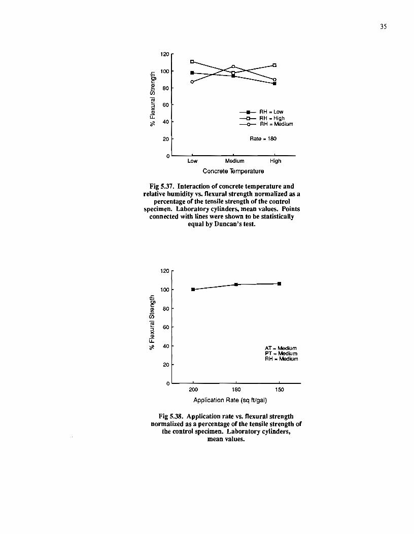
.r::.

~ 2!

Ci5 "iii .... ::I )( Q)

u::: ~ 0

120

100

80

60 _._ RH=Low -o- RH=High

40 --o-- RH =Medium

20 Rate- 180

0~--~--------~----------._ __ __ Low Medium

Concrete lemperature

High

Fig 5.37. Interaction of concrete temperature and relative humidity vs. flexural strength normalized as a

percentage of the tensile strength of the control specimen. Laboratory cylinders, mean values. Points

connected with lines were shown to be statistically equal by Duncan's test.

120

• • 100 .... .r::. c, c: so 2!

Ci5 -e 60 ::I )( Q)

u::: :.11 0

40 AT- Medium PT- Medium RH .. Medium

20

0 200 180 150

Application Rate (sq ftlgal)

Fig 5.38. Application rate vs. flexural strength normalized as a percentage of the tensile strength of

the control specimen. Laboratory cylinders, mean values.

35

CHAPTER 6. CONCLUSIONS AND RECOMMENDATIONS

CONCLUSIONS Based upon the experimental results the following

conclusions can be made:

(1) For application rates of the membrane curing com­pound between 150 to 200 square feet per gallon it can be concluded that (a) the application rate does not have a significant

effect on the tensile strength of pavement concrete as measured by the splitting tensile strength test performed on cores extracted from pavement slabs. This applies for the full depth of the pavement, and for temperature, humidity, and wind conditions resulting in evaporation rates of 0.03 to 0.28 lbs per hour per square foot as defined by the Portland Cement Association;

(b) the application rate does not have a significant effect on the surface durability of pavement concrete as measured by the sandblast abra­sion test;

(c) the application rate does not have a significant effect on the density of the pavement con­crete. This applies for the full depth of the pavement; and

(d) the application rate does not have a significant effect on the flexural or the tensile strength of specimens prepared in the field under casting and curing conditions similar to those of the actual pavement.

(2) Spectral Analysis of Surface Waves (SASW) is a feasible in-situ, non-destructive method that can be used to monitor the stiffness gain of fresh concrete with an accuracy that may be favorably compared to

36

that of the traditional large-strain method of measuring the modulus of elasticity. Both these methods showed that an increase in the membrane curing compound application rate may result in an increase in the stiff­ness of pavement concrete.

(3) The P-wave method for the measurement of the modu­lus of elasticity, when used on cores extracted from concrete pavement, did not offer any conclusive re­sults.

(4) Laboratory tests gave conflicting and inconclusive results in regards to the effects of the membrane curing compound application rate and of temperature and humidity curing conditions on the flexural and tensile strength of beams and cylinders, respectively. There­fore no correlation of laboratory and field test is possible.

RECOMMENDATIONS Based upon the experimental results, the following

recommendations can be made:

(1) The membrane curing compound application rate of 180 square feet per gallon specified for highway pave­ments was found to be slightly conservative. It would therefore be possible to decrease it to 200 square feet per gallon without any significant loss on tensile or flexural strength, surface durability, and density re­gardless of environmental conditions.

(2) Spectral Analysis of Surface Waves (SASW) method should be further investigated and developed as an in­situ, non-destructive method for quality control of both fresh and cured concrete, as well as a method to be used in studying the material properties of concrete in general.

REFERENCES 1. "Standard Practice for Curing Concrete," ACI Stan- Annual Book: of ASTM Standards, Vol 04.02, pp

dard 308-81, American Concrete Association, 281-284. Chicago, 1981. 14. ASTM C642-82, Standard Test Method for Specific

2. AASHTO Materials, Part 1: Specifications, 13th ed., Gravity, Absorption, and Voids in Hardened Con-American Association of Highway and Transpor- crete, 1986 Annual Book of ASTM Standards, Vol tation Officials, Washington, D.C., 1982. 04.02, pp 403-405.

3. ASTM C156-80a, Standard Test Method for Water 15. GlenJ. Rix, "Experimental StudyofFactorsAffecting Retention by Concrete Curing Materials, Ameri- the Spectral-Analysis-of-Surface-Waves can Society for Testing and Materials, 1986 An- Method," Dissertation, The University of Texas at nual Book of ASTM Standards, Vol 04.02, p 123. Austin, 1988, pp 31-65.

4. "1982 Standard Specifications for Construction of 16. ASTM C469-83, Standard Test Method for Static Highways, Streets and Bridges," Texas State Modulus of Elasticity and Poisson's Ratio of Department of Highways and Public Transporta- Concrete in Compression, American Society for tion. Testing and Materials, 1986 Annual Book of

5. R.E. Carrier and P.D. Cady, "Evaluating Effectiveness ASTM Standards, Vol 04.02, pp 305-309.

of Concrete Curing Compounds," Journal of Mate- 17. ASTM C39-86, Standard Test Method for Compres-rials,JMLSA, Vol5,No.2,June 1970,pp294-302. sive Strength of Cylindrical Concrete Specimens,

6. T.C. Powers, "A Discussion of Cement Hydration in American Society for Testing and Materials, 1986

Relation to Curing of Concrete," Proceedings, Annual Book of ASTM Standards, Vol 04.02, pp

Highway Research Board, HIPRA, Vol27, 1947, 24-28.

pp 178-189. 18. ASTM C143-78, Standard Test Method for Slump of

7. Chryssis G. Papaleontiou, Matthew D. Loeffler, Alvin Portland Cement Concrete, 1986 Annual Book of

H. Meyer, and David W. Fowler, '"The Effective- ASTM Standards, Vol 04.02, pp 109-111.

ness of Texas Membrane Curing Compound Qual- 19. ASTM C231-82, Standard Test Method for Air Con-ity and Application Requirements," Research tent of Freshly Mixed Concrete by the Pressure Report 427-1F, Center for Transportation Re- Method, 1986 Annual Book of ASTM Standards, search, The University of Texas at Austin, June Vol 04.02, pp 169-178. 1986. 20. ASTM C29-78, Standard Test Method for Unit

8. Seyed Mehdi Samsam Shariat and Prahlad D. Pant, Weight and Voids in Aggregate, 1986 Annual "Curing and Moisture Loss of Grooved Concrete Book: of ASTM Standards, Vol 04.02, pp 1-4. Surfaces," Transportation Research Record, 1986, 21. Tex 420-A,loc cit pp4-8.

22. ASTM C496-85,loc cit. 9. Ronald Q. Wrbas, William B. Ledbetter, and Alvin H.

Meyer, "Effectiveness of Membrane Curing on 23. ASTM C496-85, loc cit.

Concrete Surfaces," Highway Research Record, 24. Tex 420-A, loc cit 433, pp 23-34. 25. "Curing of Concrete," Concrete Information Sheet IS

10. ASTM C496-85, Standard Test Method for Splitting 55.02 T, Portland Cement Association, Chicago, Tensile Strength of Cylindrical Concrete Speci- 1966. mens, American Society for Testing and Materials, 26. Wrbas et al, Joe cit. 1986 Annual Book of ASTM Standards, Vol

27. Papaleontiou et al, loc cit 04.02, pp 337-339.

11. Powers,loc cit 28. Sidney Mindess and J. Francis Young, Concrete

12. Tex 420-A, Flexural Strength of Concrete Using (Englewood Oiffs, NJ.: Prentice-Hall, 1981), p 303.

Simple Beam with Center-Point Loading, State 29. ASTM C192-81, Standard Method for Making and Department of Highways and Public Transporta-

tion, Materials and Tests Division. Curing Concrete Test Specimens in the Labora-

13. ASTM C418-81, Standard Test Method for Surface tory,1986 Annual Book of ASTM Standards, Vol

Durability by the Sandblast Abrasion Tesa.1986 04.02, pp 142-143.

37

38

30. Virgil L. Anderson and Robert A. McLean, Design of Experiments, A Realistic Aproach (New York: Marcel Dekker, Inc., 1974), p 40.

31. SAS Institute Inc., SAS/STAT™Guide for Personal Computers, Version 6 Edition, Cary, NC: SAS Institute Inc., 1985. 378 pp.

APPENDIX A. FIELD EXPERIMENT RESULTS

TABLE A.l. SPLIT TENSILE TEST RESULTS ON 2-INCH SLICES OF CORES OBTAINED IN THE FIELD. SITE #1, TULIA, TEXAS. ALL VALUES

IN PSI.

CORE CONTR SECT RATE POS 1 2

EX B 434 556 T 431 442

POLY B 467 399

S1 T 520 475

150 B 595 460 T 542 555

N1 200 B 355 496 T 417 550

180 B 443 492 T 525 488

180 B 555 407 T 585 503

S2 B • 460 200 T 494 535

• Damaged specimen

TABLE A.2. SPLIT TENSILE TEST RESULTS ON 2-INCH SLIDES OF CORES OBTAINED IN THE FIELD. SITE #2, TULIA, TEXAS. ALL VALUES

IN PSI.

CORE CONTR SECT RATE POS 1 2

B 480 463 EX T 377 479

POLY B 454 387

S1 T 419 419

150 B 544 457 T 557 •

N2 180 B 526 423 T 462 547

200 B 554 493 T 467 481

180 B 509 403 T 503 400

S2 200 B 463 430

T 429 458

• Damaged specimen

39

40

TABLE A.3. SPLIT TENSILE TEST RESULTS ON 2-INCH SLICES OF CORES OBTAINED IN THE FIELD. SITE #3,

FORT WORTH, TEXAS. ALL VALUES IN PSI.

CORE CONTR SECT RATE POS 1 2 3 4

EX B - - - 608 T 414 633 452 538 B 657 560 693 -POLY T 710 589 409 551 S1

150 B - 643 611 -T 662 480 735 542

N3 180 B - 551 530 625 T 711 526 681 628 B - - 567 506

200 T 540 618 701 623

Ex B - 440 547 -T 465 536 474 *

150 B 650 693 521 584 T * 650 626 367 S2

180 B . 805 - 761 T * 480 559 382

200 B 518 - 557 530 T 503 * 477 *

* Damaged specunen - Specimen severely honeycombed possibly due to

undervibration. Not tested

TABLE A.4(A). SPLIT TENSILE TEST RESULTS ON 2-INCH SLICES OF CORES

OBTAINED IN THE FIELD. SITE #4 AND S, HOUSTON, TEXAS. ALL VALUES IN PSI.

mRi CONTR SECT RATE POS 1

B 728

DRY M1 661 M2 810 T 683 B *

EX Ml 615 M2 763

Sl T 658 B *

POLY M1 552 M2 793 T 771 B 693

N4 Ml 645 M2 580

150 T 701 B 859

M1 771 M2 767 T tiRii B 783

200 Ml 804 M2 854 T 800 B 679

S2 180 Ml 767 M2 778 T 812

* Damaged specunen

TABLE A.4(B). SPLIT TENSILE TEST RESULTS ON 2-INCH SLICES OF CORES

OBTAINED IN THE FIELD. SITE #4 AND 5, HOUSTON, TEXAS. ALL VALUES IN PSI.

tORE CONTR SECT RATE POS 1

B 633 M1 674

DRY M2 777 T 695 B 678

EX M1 680 M2 * T 699 B 649

POLY M1 699 M2 768

Sl T 698 B 727

150 Ml 726 M2 745 T 688 B 674

180 M1 730 M2 573 T n"i7 B 722

N5 200 M1 678 M2 707 T R7? B 754

Dry M1 730 M2 793 T 7"i7 B 738

Ex Ml 763 M2 718 T 852 B 727

S2 150 M1 739 M2 745 T 797 B 773

M1 794 180 M2 833

T 688 B 661

200 M1 709 M2 808 T 741

* Damaged specimen

41

42

TABLE A.S. SPLIT TENSILE TEST RESULTS ON 2-INCH SLICES OF CORES OBTAINED IN THE FIELD. SITE #6, EL PASO,

TEXAS. ALL VALUES IN PSI.

~ CONTR SECT RATE POS 1

B 561

Dry M1 503 M2 553 T 383 B 375

Ex Ml 453 M2 485 T 523 B 511

Poly Ml 510 M2 491 T 507 .H 571

N6 S1 150 M1 415 M2 567 T liQ':\ B 597

180 M1 438 M2 597 T 380 B 578

200 M1 514 M2 481 T 383 B 504

250 M1 413 M2 481 T 432

TABLE A.6. SPLITTING TENSILE STRENGTH OF 6-INCH X 12-INCH CYLINDERS PREPARED AND CURED IN THE FIELD (PSI)

Contractor

1 2 3 4 5 6 AppUcation Rate, Sect Sect Sect Sect Sect Sect Sect

sq ft/gal 1 2 3 4 5 6 7

Dry 624 626 442

200 469 460 513 465 590 607 436 488 491 460

180 497 394 504 466 651 617 453 518 450 462 470 566 660 504

150 485 403 505 488 671 589 460 720 445 460

TABLE A.7. FLEXURAL STRENGTH OF 6-INCH X 21-INCH BEAMS PREPARED AND CURED IN THE FIELD (PSI)

I

Contractor

1 2 3 4 5 Application Rate, Sect Sect Sect Sect Sect Sect

sq ft/gal 1 2 3 4 5 6

Dry 865 865

200 743 625 560 590 1005 920 655 690 510 1005 920

180 670 610 675 625 890 900 715 620 710 470 1095 810

150 I 110 I 720

685 I 120 I 650 615

635 I 860 I 750 I

TABLE A.8. RESULTS FROM SURFACE DURABILITY TEST PERFORMED ON 4-INCH

CORES (TOP SURFACE AREA 10.9 SQ IN.) (GRAMS)

Contractor

Application Rate, sq ft/gal 4 5

Dry 3.12 3.27 5.38*

250

200 3 3.21

2.70*

180 3.41 4.42 2.99*

Ex 2.96 3.13

2.84•

150 431 2.92*

Poly 3.94 3.56

• Values from the repeat sa:tion from contractor ItS.

6

4.40

4.50

5.40

4.50

4.40

3.20

4.00

6 Sect

7

620

680 680

695 660

665

43

44

TABLE A.9. DENSITY AT TOP AND BOTTOM 2 INCHES OF CORES EXTRACTED FROM SITES #1 AND #2 (SEE TABLE 2.2) (LBS/CU FT)

Contractor 1 2

Location Location

AppUcatlon Rate sq tt/gal SECT CORES Top ~ttom Top Bottom

1 1 144.89 140.15 144.46 144.27

180 1 2 147.08 141.52 141.02 141.59 2 1 143.83 143.89 148.02 139.59 2 2 144.21 142.77 140.40 142.40

1 1 146.52 139.78 143.46 142.96 1 2 141.90 148.64 145.83 145.20

200 2 1 143.02 157.50 140.34 143.15 2 2 145.27 140.09 142.27 143.08

150 1 1 146.95 141.34 143.96 141.90 1 2 146.14 142.96 138.22 142.58

EX 1 1 143.58 142.02 143.83 143.58 1 2 142.46 141.46 145.45 146.27

POLY 1 1 145.20 140.46 144.64 142.33 1 2 145.77 140.77 140.84 143.83

APPENDIX B. ANALYSIS OF VARIANCE RESULTS FOR FIELD EXPERIMENT

TABLE B.l. SUMMARY OF ANOVA OF SPLITTING TENSILE TEST RESULTS ON 2-INCH SLICES FROM CORES OBTAINED FROM THE FIELD (MODEL lA)

Classification of Variables

Class Level Values

CONTR 6 N1 N2 N3 N4 N5 N6 RATE 7 DRY EX POLY 150 180 200 250 SECT 2 S1 S2 POS 4 T M1 M2 B CORE 4 1 2 3 4

Source DF FValue Pr* Significance

a=O.lO CONTR 5 32.4 <0.01 Yes SECT(CONTR) 5 1.76 0.18 No

a 0 RATE 6 1.32 0.25+ No CONTR*RATE 22 1.45 0.25+ No RATEe*SECT(CONTR) 9 0.75 0.25+ No CORE(CONTR*RATE*SECT) 38 1.04 0.25+ No (I) 0 POS 3 1.07 0.25+ No CONTR*POS 9 1.16 0.25+ No SECTt*POS(CONTR) 9 1.24 0.25+ No RATE*POS 18 0.84 0.25+ No CONTR*RATE*POS 40 0.88 0.25 + No RATE*SECT*POS(CONTR) 16 1.11 0.25+ No ERROR 23 * Probability of rejection value associated with the F value

45

46

TABLE B.2. SUMMARY OF ANOV A OF SPLITTING TENSILE TEST RESULTS ON 2-INCH SLICES FROM CORES OBTAINED FROM THE FIELD (MODEL lB)

Classification or Variables Class Level Values

CONTR 3 N4 N5 N6 RATE 7 DRY EX POLY 150 180 200 250 SECT 2 S1 S2 POS 4 T M1 M2 B CORE

Source DF FValue Pr* Significance

a= 0.10

CONTR 2 25.76 0.05 Yes SECT(CONTR) 2 0 RATE 6 0.56 0.25+ No CONTR*RATE 10 1.32 0.25+ No RATE*SECT(CONTR) 4 CORE(CONTR*RATE*SECT) (I) 0 POS 3 1.93 0.24 No CONTR*POS 6 1.02 0.25+ No SECT*POS(CONTR) 6 1.57 RATE*POS 18 0.10 0.25+ No CONTR*RATE*POS 29 1.58 0.23 No RATE*SECT*POS(CONTR) 11 1.62 POS*CORE(CONTR*RATE*SECT) 0

• Probability of rejection value associated with the F value

TABLE B.J. SUMMARY OF ANOV A OF SPLITTING TENSILE TEST RESULTS ON 2-INCH SLICES FROM CORES OBTAINED FROM THE FIELD (MODEL lC)

Classification or Variables Class Level Values

CONTR 3 N4 N5 N6 RATE 7 DRY EX POLY 150 180 200 250 SECT 2 S1 S2 POS 4 T M1 M2 B CORE 1 1

Source DF FValue ~ Significance

a= 0.10

CONTR 2 25.76 0.05 Yes SECT(CONTR) 2 0 RATE 6 0.56 0.25+ No CONTR*RATE 10 1.32 0.25+ No RATE*SECT(CONTR) 4 CORE(CONTR*RATE*SECT) (I) 0 POS 3 1.93 0.24 No CONTR*POS 6 1.02 0.25+ No SECT*POS(CONTR) 6 1.57 RATE*POS 18 0.10 0.25+ No CONTR*RATE*POS 29 1.58 0.23 No RATE*SECT*POS(CONTR) 11 1.62 POS*CORE(CONTR*RATE*SECT) 0

• Probability of rejection value associated with the F value

TABLE 8.4. SUMMARY OF ANOVA OF SPLITTING TENSILE TEST RESULTS ON 2-INCH SLICES FROM CORES OBTAINED FROM THE FIELD (MODEL lD)

Classification or Variables Class Level Values

CONTR 6 N1 N2 N3 N4 N5 N6 RATE 7 DRY EX POLY 150 180 200 250 SECT 2 S1 S2 POS 4 T M1 M2 B CORE 4 1 2 3 4

Source DF FValue Pr* Significance

a= 0.10 -CONTR 5 12.26 O.Dl Yes SECT(CONTR) 5 1.16 0.25+ No a 0 RATE 6 1.56 0.22 No CONTR*RATE 22 1.92 0.18 No RATE*SEcr(CONTR) 9 0.50 0.25+ No CORE(CONR*RATE*SECT) 38 1.04 0.25 + No (I) 0 POS 3 0.91 0.25+ No CONTR*POS 9 1.46 0.25+ No SECT*POS(CONTR) 9 0.94 0.25+ No RATE*POS 18 0.73 0.25+ No CONTR*RATE*POS 40 1.24 0.25+ No RATE*SEcr*POS(CONTR) 16 0.88 0.25+ No ERROR 23 • Probability of rejection value associated with the F value

TABLE B.S. SUMMARY OF ANOV A OF SPLITTING TENSILE TEST RESULTS ON 2-INCH SLICES FROM CORES OBTAINED FROM THE FIELD. NORMALIZED DATA.

ENVIRONMENTAL EFFECTS INCLUDED. (MODEL lE)

Classification or Variables

~ !:!!!!.. Values

CONTR 5 N1 N2 N3 N4 N5 RATE 6 DRY EX POLY 150 180 200 250 SECT 2 S1 S2 POS 4 T M1 M2 B CORE 4 1 2 3 4 EVAP 7 0.3 0.03 0.14 0.22 0.23 0.25 0.28

Significance Source .!!! F Value ~ a =0.10

CONTR 4 3.20 0.13 No SECT(CONTR) 5 1.34 0.25+ No a 0 EVAP(CONTR*SECT) 0 RATE 5 1.23 0.25 + No CONTR*RATE 17 2.11 0.14 No RATE*EVAP(CONIR*SECI') 9 0.42 0.25+ No (I) 0 POS 3 0.40 0.25 + No CONTR*POS 6 1.17 0.25+ No POS*EVAP(CONTR *SECT) 9 1.16 0.25+ No RATE*POS 15 0.98 0.25+ No CONTR*RATE*POS 25 0.50 0.25+ No ERROR 77

• Probability of rejection value associated with the F value

47

48

TABLE B.6. SUMMARY OF ANOV A OF SPLITTING TENSILE TEST RESULTS ON 2-INCH SLICES FROM CORES OBTAINED

FROM THE FIELD (MODEL 2A)

Classification of Variables Class Level Values --CONTR 6 N1 N2 N3 N4 N5 N6 RATE 7 DRY EX POLY 150 180 200 250 SECT 2 S1 S2 POS 4 T Ml M2 B

Source DF FValue Pr* Significance

a= 0.10 ---CONTR 5 26.78 < O.Ql Yes SECT(CONTR) 5 1.21 0.25+ No 0 0 RATE 6 1.39 0.25+ No CONTR*RATE 22 1.21 0.25+ No RATE*SECT(CONTR) 9 0.79 0.25+ No (I) 0 POS 3 0.96 0.25+ No CONTR*POS 9 130 0.25+ No SECT*POS(CONTR) 9 1.20 0.25+ No RATE*POS 18 1.81 0.25+ No CONTR*RATE*POS 40 0.77 0.25+ No RATE*SECT*POS(CONTR) 16 1.20 0.25+ No ERROR 61

* Probability of rejection value associated with the F value

TABLE B.7. SUMMARY OF ANOVA OF SPLITTING TENSILE TEST RESULTS ON 2-INCH SLICES FROM CORES OBTAINED

IN THE FIELD (MODEL 2B)

Classification of Variables Class 1!!!1. Values

CONTR 3 N4 N5 N6 RATE 7 DRY EX POLY 150 180 200 250 SECT 2 S1 S2 POS 4 T M1 M2 B

Source ~ FValue Significance

Pr* a= 0.10 CONTR 2 25.03 0.05 Yes SECT(CONTR) 2 RATE 6 1.67 0.24 No CONTR*RATE 10 1.31 0.25+ No RATE*SECT(CONTR) 4 POS 3 1.76 0.25+ CONTR*POS 6 1.11 0.25+ No SECT*POS(CONTR) 6 1.57 0.25 No RATE*POS 18 1.03 0.25+ No CONTR*RATE*POS 28 1.58 0.23 No RATE*SECT*POS(CONTR) 11

* Probability of rejection value associated with the F value

TABLE 8.8. SUMMARY OF ANOV A OF SPLITTING TENSILE TEST RESULTS ON 2-INCH SLICES FROM CORES OBTAINED

FROM THE FIELD (MODEL 2C)

Classification of Variables Class Level Values

CONfR 6 Nl N2 N3 N4 N5 N6 RATE 7 DRY EX POLY 150 180 200 250 SECT 2 S1 S2 POS 2 TB

Source DF FValue Pr• Significance

a =0.10

CONfR 5 32.2 < O.Ql Yes SECT(CONTR) 5 2.03 0.08 Yes

s 0 RATE 6 1.83 0.16 No CONfR*RATE 22 0.98 0.25+ No RATE*SECT(CONfR) 9 0.86 .0.25 + No (1) 0 POS 1 CONfR*POS 5 1.27 0.25+ No SECT*POS(CONfR) 5 1.94 0.09 Yes RATE*POS 6 1.13 0.25+ No CONfR*RATE*POS 20 0.64 0.25+ No RATE*SECT*POS(CONfR) 9 1.62 0.12 No ERROR 61

• Probability of rejection value associated with the F value

TABLE 8.9. SUMMARY OF ANOVA OF SPLIT CYLINDER TEST RESULTS ON 6-INCH X 12-INCH

CYLINDERS OBTAINED FROM THE FIELD

Classification of Variables Class Level Values

CONTR 6 Nl N2 N3 N4 N5 N6 RATE 4 DRY 150 180 200 SECT 2 S1 S2

Significance Source DF Fvalue Pr• a= 0.10 ---

CONTR 5 127 <0.01 Yes SECT(CONTR) 1

s 0 RATE 3 0.34 0.25+ No CONTR*RATE 12 7.82 0.14 No SECT*RATE(CONTR) 2 0.11 0.25+ No ERROR 12

* Probability ofrejection value associated with the F value

49

50

TABLE B.10. SUMMARY OF ANOVA OF SPLIT CYLINDER TEST RESULTS ON 6-INCH X 12-INCH CYLINDERS OBTAINED FROM

THE FIELD. NORMALIZED VALUES.

Classification of Variables Class

CONTR RATE SEer

Level Values

6 Nl N2 N3 N4 N5 N6 4 DRY 150 180 200 2 Sl S2

Source DF FValue CONTR 5 57 SECf(CONTR) 1 0.20 a 0 RATE 3 0.29 CONTR*RATE 12 7.38 SECf*RATE(CONTR) 2 0.12 ERROR

Pr* SignifiCance

a :0.10 <0.01 Yes 0.25+ No

0.25+ No 0.16 No 0.25+ No

• Probability of rejection value associated with the F value

TABLE B.ll. SUMMARY OF ANOV A OF FLEXURE TEST RESULTS ON 6-INCH X 12-INCH

BEAMS OBTAINED FROM THE FIELD

Classification of Variables Class le:.;!. Values

CONTR 6 Nl N2 N3 N4 N5 N6 RATE 4 DRY 150 180 200 SEer 2 Sl S2

Source OF FYalue Pr• Significance

a=0.10

CONTR 5 400 <0.01 Yes SECf(CONTR) 1 3 0 RATE 3 0.46 0.25+ No CONTR*RATE 12 1.61 0.25+ No SECT*RJU'E(CONTR) 2 0.92 0.25+ No ERROR

• Probability of rejection value associated with the F value

TABLE B.U. SUMMARY OF ANOVA OF FLEXURE TEST RESULTS ON 6-INCH X 21-INCH

BEAMS OBTAINED FROM THE FIELD. NORMALIZED VALUES.

Classification of Variables Class Level Values

CONTR 6 N1 N2 N3 N4 N5 N6 RATE 4 DRY 150 180 200 SECf 2 S1 S2

Souree DF FValue Pr• Sign.if1cance

a=0.10 ----CONTR 5 219 <0.01 Yes SECf(CONTR) 1 0.08 0.25 + No

a 0 RATE 3 0.41 0.25 + No CONTR*RATE 12 1.17 0.25 + No SECf•RATE(CONTR) 2 1.23 0.25 + No ERROR

• Probability of rejection value associated with the F value

TABLE B.13. SUMMARY OF ANOVA OF SURFACE DURABILITY TEST RESULTS ON 2-INCH SLICES

FROM CORES OBTAINED FROM THE FIELD (MODELD4)

Classification of Variables Class

CONTR RATE SEer

Level Values

3 N4 N5 N6 7 DRY EX POLY 150 180 200 250 2 Sl S2

Souree DF F Value Pr• Significance

a= 0.10 --CONTR 2 5.54 0.25+ No SECf(CONTR) 1

a RATE 6 0.52 0.25+ No CONTR*RATE 8 0.49 0.25+ No RATE*SECf(CONTR) -• Probability of rejection value associated with the F value

51

52

TABLE B.l4. SUMMARY OF ANOV A OF DENSITY TEST RESULTS ON 2-INCH SLICES FROM CORES OBTAINED FROM THE FIELD

(MODEL DS)

Classification of Variables Class Level Values

CONTR 2 N1 N2 RATE 5 EX POLY 150 180 200 SECT 2 S1 S2 POS 2 T B CORE 2 1 2

Source OF FValue Pr• Signifjcance

a= 0.10 ----CONTR 1 4.55 0.200 No SECT(CONTR) 2

s RATE 4 0.52 0.25 + No CONTR*RATE 4 1.15 RATE*SECT(CONTR) 2 0.87 CORE(CONTR*RATE*SECT) 14 (I)

POS 1 1.10 0.25+ No CONTR*POS 1 0.33 0.25+ No SECT*POS(CONTR) 2 1.09 0.25+ No RATE*POS 4 2.83 0.128 No CONTR*RATE*POS 4 0.74 0.25 + No RATE*SECT*POS(CONTR) 2 0.33 0.25+ No POS*CORE(CONTR*RATE*SECT) 14

• Probability of rejection value associated with the F value

APPENDIX C. SPECTRAL ANALYSIS OF SEISMIC WAVES (SASW) RESULTS

TABLE C.1. SASW TESTING SCHEDULE. ALL TIMES IN MINUTES AFTER CONCRETE MIXING.

Test Test Test Test Test Test Test Test Panel Rate #1 #2 #3 #4 #S #6 #7 #8

1 DRY 190 245 369 434 544 770 1486 8160 2 150 272 393 560 775 1508 8221 3 250 214 420 600 790 1530 8230 4 180 299 464 573 806 1542 8240 7 200 340 519 639 827 1563 8250

TABLE C.l. YOUNG'S MODULUS. AVERAGE VALUES FOR RECEIVER SPACINGS OF 1.00 Ff AND

WAVELENGTHS OF 0.25, 0.50, AND 0.75 FOOT. ALL VALUES IN PSI X 10'.

Test Test Test Test Test Test Test Test Panel Rate #1 #2 #3 #4 #S #6 #7 #8 - --

1 DRY 0.43 0.98 2.09 2.51 3.26 3.84 4.23 4.35 2 150 1.31 2.96 2.98 4.21 4.60 4.90 3 250 0.23 2.01 3.31 3.70 4.14 4.40 4 180 1.16 3.00 3.25 3.95 4.56 4.60 7 200 1.00 2.63 2.92 3.32 3.88 4.15

TABLE C.3. YOUNG'S MODULUS. AVERAGE VALUES FOR RECEIVER SPACINGS OF 0.50 FT AND

WAVELENGTHS OF 0.25, 0.50, AND 0.75 FOOT. ALL VALUES IN PSI X 10'.

Test Test Test Test Test Test Test Test Panel Rate #1 #2 #3 #4 #S #6 #7 #8

1 DRY ... ... ... ... ... ... ... ... 2 150 1.17 2.47 - 3.22 3.92 4.51 4.49 3 250 ... ... ... ... ... ... 4 180 0.96 2.51 3.22 3.53 4.19 4.37 7 200 ... ... ... ... ... ...

53

APPENDIX D. LABORATORY EXPERIMENT RESULTS

TABLE D.l. LABORATORY EXPERIMENT. SPLIT TENSILE TEST, 6-INCH X 12-INCH CYLINDERS. ALL VALUES IN PSI. CYLINDER "A" IS THE CONTROL SPECIMEN.

Rate

200 180 ISO Cylinder CyHnder Cylinder

AT CT RH #1 #2 #3 N #1 #2 #3 N #I #2 #3 N High

High Med Low 426 494 461 490

High

High Med Med Low 382 426 397 475

High

Low Med Low 382 359 375 428

High 477 498 427 411 High Med 439 386 404 407

Low

High 476 413 431 513 Med Med Med 433 468 408 431 406 409 404 470 361 373 402 417

Low

High 448 416 387 421 Low Med 446 448 393 413

Low

54

TABLE D.2. LABORATORY RESULTS, 6-INCH X 12-INCH CYLINDERS. NORMALIZED DATA. ALL VA LUES REPRESENT PERCENTAGES OF THE SPLIT TENSILE STRENGTH

OF THE CONTROL CYLINDER OF EACH BATCH. (DESIGNATED AS SPECIMEN ''N")

Rate

200 180 150 Cylinder CyUnder Cylinder

AT CT RH #1 #2 #3 N #1 #2 #3 N #1 #2 #3 N High

High Med Low 87 101 94 100

High

High Med Med Low 80 90 84 100

High

Low Med Low 89 84 88 100

High 116 121 104 100 High Med 108 95 99 100

Low

High 93 82 84 100 Med Med Med 100 109 95 100 86 87 86 100 87 89 96 100

Low

High 106 99 92 100 Low Med 108 108 95 100

Low

55

56

TABLE D.3. LABORATORY RESULTS. FLEXURE TEST, 6-INCH X 12-INCH BEAMS. ALL VALUES IN PSI. BEAM ''N" IS THE CONTROL SPECIMEN.

Rate 200 180 150

Cylinder Cylinder Cylinder

AT CT RH #1 #2 #3 N #1 #2 #3 N #1 #2 #3 N High

High Med Low 587 570 540 670

High

High Med Med Low 567 590 610 630

High

Low Med Low 587 695 585 633

High 680 690 650 630 High Med 655 600 510 650

Low

High 655 665 690 685 Med Med Med

Low

High 773 640 660 625 Low Med 590 600 535 660

Low

TABLE D.4. LAB ORA TORY RESULTS. 6-INCH X 21-INCH BEAMS. NORMALIZED DATA. ALL VALUES ARE PERCENT AGES OF THE FLEXURAL STRENGTH OF THE CONTROL

BEAM OF EACH BATCH. (DESIGNATED AS SPECIMEN)

Rate

200 180 150 Cylinder Cylinder Cylinder

AT CT RH #1 #2 #3 N #1 #2 #3 N #1 #2 #3 N Hlgb

Hlgb Med Low 88 85 81 100

Hlgb

Hlgb Med Med Low 90 94 97 100

Hlgb

Low Med Low 93 110 92 100

Hlgb 108 110 103 100 Hlgb Med 101 92 78 100

Low

Hlgb 96 97 101 100 Med Med Med 101 96 104 100 104 111 100 100 107 103 108 100

Low

Hlgb 124 102 106 100 Low Med 89 91 81 100

Low

57

APPENDIX E. ANALYSIS OF VARIANCE RESULTS FOR THE LABORATORY EXPERIMENT

TABLE E.l. SUMMARY OF ANOVA OF FLEXURAL STRENGTH TEST RESULTS ON 6-INCH X 21-INCH

CYLINDERS PREPARED IN THE LABORATORY (MODEL SA)

Classification of Variables

Class ~ Values

AT 2 HM CT 3 HML RH 2 HML

Significance

~ m: FValue ~ a""'O.lO

AT 0 CT 2 17.5 <O.ot Yes RH 1 0.91 0.25+ No CT*RH 4 2.94 0.05 Yes Error 18

* Probability of rejection value associated with the Fvalue

TABLE E.2. SUMMARY OF ANOV A OF FLEXURAL STRENGTH TEST RESULTS ON 6-INCH X 21-INCH

CYLINDERS PREPARED IN THE LABORATORY (MODELSB)

Classification of Variables Class Levels Values ---RATE 3 200 180 150

Significance Source DF F Value Pr* a= 0.10 ---RATE 2 4.70 0.05 Yes ERROR 6

* Probability of rejection value associated with the F value

58

TABLE E.J. SUMMARY OF ANOVA OF FLEXURAL STRENGTH TEST RESULTS ON 6-INCH X ll-INCH BEAMS

PREPARED IN THE LABORATORY (MODEL SA)

Classification of Variables Class ~ ~ AT 2 HM cr 3 HML RH 2 HML

Significance Source DF FValue Pr* a= 0.10 AT 0 cr 2 1.29 0.25+ No RH 1 10.5 <0.01 Yes Cf*RH 4 4.51 0.01 Yes ERROR 18

* Probability of rejection value associated with the F value

TABLE E.4. SUMMARY OF ANOVA OF FLEXURAL STRENGTH TEST RESULTS ON 6-INCH X ll-INCH BEAMS

PREPARED IN THE LABORATORY (MODEL 58)

Classification of Variables Class Levels Values RATE 3 200 180 150

Source DF

RATE 2 ERROR 6

FValue Pr*

0.52 0.25 +

Significance a =0.10

No

* Probability of rejection value associated with the F value

59