arX

iv:1

111.

7122

v1 [

astr

o-ph

.IM

] 3

0 N

ov 2

011 The effect of the geomagnetic field on cosmic ray energy

estimates and large scale anisotropy searches on data from

the Pierre Auger Observatory

The Pierre Auger Collaboration

P. Abreu74, M. Aglietta57, E.J. Ahn93, I.F.M. Albuquerque19, D. Allard33, I. Allekotte1, J. Allen96,P. Allison98, J. Alvarez Castillo67, J. Alvarez-Muniz84, M. Ambrosio50, A. Aminaei68, L. Anchordoqui109,S. Andringa74, T. Anticic27, A. Anzalone56, C. Aramo50, E. Arganda81, F. Arqueros81, H. Asorey1,P. Assis74, J. Aublin35, M. Ave41, M. Avenier36, G. Avila12, T. Backer45, M. Balzer40, K.B. Barber13,A.F. Barbosa16, R. Bardenet34, S.L.C. Barroso22, B. Baughman98 f , J. Bauml39, J.J. Beatty98,B.R. Becker106, K.H. Becker38, A. Belletoile37, J.A. Bellido13, S. BenZvi108, C. Berat36, X. Bertou1,P.L. Biermann42, P. Billoir35, F. Blanco81, M. Blanco82, C. Bleve38, H. Blumer41, 39, M. Bohacova29,D. Boncioli51, C. Bonifazi25, 35, R. Bonino57, N. Borodai72, J. Brack91, P. Brogueira74, W.C. Brown92,R. Bruijn87, P. Buchholz45, A. Bueno83, R.E. Burton89, K.S. Caballero-Mora99, L. Caramete42,R. Caruso52, A. Castellina57, O. Catalano56, G. Cataldi49, L. Cazon74, R. Cester53, J. Chauvin36,S.H. Cheng99, A. Chiavassa57, J.A. Chinellato20, A. Chou93, J. Chudoba29, R.W. Clay13, M.R. Coluccia49,R. Conceicao74, F. Contreras11, H. Cook87, M.J. Cooper13, J. Coppens68, 70, A. Cordier34, S. Coutu99,C.E. Covault89, A. Creusot33, 79, A. Criss99, J. Cronin101, A. Curutiu42, S. Dagoret-Campagne34,R. Dallier37, S. Dasso8, 4, K. Daumiller39, B.R. Dawson13, R.M. de Almeida26, M. De Domenico52,C. De Donato67, 48, S.J. de Jong68, 70, G. De La Vega10, W.J.M. de Mello Junior20, J.R.T. deMello Neto25, I. De Mitri49, V. de Souza18, K.D. de Vries69, G. Decerprit33, L. del Peral82,M. del Rıo51, 11, O. Deligny32, H. Dembinski41, N. Dhital95, C. Di Giulio47, 51, J.C. Diaz95,M.L. Dıaz Castro17, P.N. Diep110, C. Dobrigkeit 20, W. Docters69, J.C. D’Olivo67, P.N. Dong110, 32,A. Dorofeev91, J.C. dos Anjos16, M.T. Dova7, D. D’Urso50, I. Dutan42, J. Ebr29, R. Engel39,M. Erdmann43, C.O. Escobar20, J. Espadanal74, A. Etchegoyen2, P. Facal San Luis101, I. FajardoTapia67, H. Falcke68, 71, G. Farrar96, A.C. Fauth20, N. Fazzini93, A.P. Ferguson89, A. Ferrero2,B. Fick95, A. Filevich2, A. Filipcic78, 79, S. Fliescher43, C.E. Fracchiolla91, E.D. Fraenkel69, U. Frohlich45,B. Fuchs16, R. Gaior35, R.F. Gamarra2, S. Gambetta46, B. Garcıa10, D. Garcıa Gamez34, 83,D. Garcia-Pinto81, A. Gascon83, H. Gemmeke40, K. Gesterling106, P.L. Ghia35, 57, U. Giaccari49,M. Giller73, H. Glass93, M.S. Gold106, G. Golup1, F. Gomez Albarracin7, M. Gomez Berisso1,P. Goncalves74, D. Gonzalez41, J.G. Gonzalez41, B. Gookin91, D. Gora41, 72, A. Gorgi57, P. Gouffon19,S.R. Gozzini87, E. Grashorn98, S. Grebe68, 70, N. Griffith98, M. Grigat43, A.F. Grillo58, Y. Guardincerri4,F. Guarino50, G.P. Guedes21, A. Guzman67, J.D. Hague106, P. Hansen7, D. Harari1, S. Harmsma69, 70,T.A. Harrison13, J.L. Harton91, A. Haungs39, T. Hebbeker43, D. Heck39, A.E. Herve13, C. Hojvat93,N. Hollon101, V.C. Holmes13, P. Homola72, J.R. Horandel68, A. Horneffer68, P. Horvath30, M. Hrabovsky30, 29,T. Huege39, A. Insolia52, F. Ionita101, A. Italiano52, C. Jarne7, S. Jiraskova68, M. Josebachuili2,K. Kadija27, K.H. Kampert38, P. Karhan28, P. Kasper93, B. Kegl34, B. Keilhauer39, A. Keivani94,J.L. Kelley68, E. Kemp20, R.M. Kieckhafer95, H.O. Klages39, M. Kleifges40, J. Kleinfeller39,J. Knapp87, D.-H. Koang36, K. Kotera101, N. Krohm38, O. Kromer40, D. Kruppke-Hansen38,F. Kuehn93, D. Kuempel38, J.K. Kulbartz44, N. Kunka40, G. La Rosa56, C. Lachaud33, P. Lautridou37,M.S.A.B. Leao24, D. Lebrun36, P. Lebrun93, M.A. Leigui de Oliveira24, A. Lemiere32, A. Letessier-Selvon35, I. Lhenry-Yvon32, K. Link41, R. Lopez63, A. Lopez Aguera84, K. Louedec34, J. Lozano

1

Bahilo83, L. Lu87, A. Lucero2, 57, M. Ludwig41, H. Lyberis32, M.C. Maccarone56, C. Macolino35,S. Maldera57, D. Mandat29, P. Mantsch93, A.G. Mariazzi7, J. Marin11, 57, V. Marin37, I.C. Maris35,H.R. Marquez Falcon66, G. Marsella54, D. Martello49, L. Martin37, H. Martinez64, O. MartınezBravo63, H.J. Mathes39, J. Matthews94, 100, J.A.J. Matthews106, G. Matthiae51, D. Maurizio53,P.O. Mazur93, G. Medina-Tanco67, M. Melissas41, D. Melo2, 53, E. Menichetti53, A. Menshikov40,P. Mertsch85, C. Meurer43, S. Micanovic27, M.I. Micheletti9, W. Miller106, L. Miramonti48, L. Molina-Bueno83, S. Mollerach1, M. Monasor101, D. Monnier Ragaigne34, F. Montanet36, B. Morales67,C. Morello57, E. Moreno63, J.C. Moreno7, C. Morris98, M. Mostafa91, C.A. Moura24, 50, S. Mueller39,M.A. Muller20, G. Muller43, M. Munchmeyer35, R. Mussa53, G. Navarra57 †, J.L. Navarro83,S. Navas83, P. Necesal29, L. Nellen67, A. Nelles68, 70, J. Neuser38, P.T. Nhung110, L. Niemietz38,N. Nierstenhoefer38, D. Nitz95, D. Nosek28, L. Nozka29, M. Nyklicek29, J. Oehlschlager39, A. Olinto101,P. Oliva38, V.M. Olmos-Gilbaja84, M. Ortiz81, N. Pacheco82, D. Pakk Selmi-Dei20, M. Palatka29,J. Pallotta3, N. Palmieri41, G. Parente84, E. Parizot33, A. Parra84, R.D. Parsons87, S. Pastor80,T. Paul97, M. Pech29, J. Pekala72, R. Pelayo84, I.M. Pepe23, L. Perrone54, R. Pesce46, E. Petermann105,S. Petrera47, P. Petrinca51, A. Petrolini46, Y. Petrov91, J. Petrovic70, C. Pfendner108, N. Phan106,R. Piegaia4, T. Pierog39, P. Pieroni4, M. Pimenta74, V. Pirronello52, M. Platino2, V.H. Ponce1,M. Pontz45, P. Privitera101, M. Prouza29, E.J. Quel3, S. Querchfeld38, J. Rautenberg38, O. Ravel37,D. Ravignani2, B. Revenu37, J. Ridky29, S. Riggi84, 52, M. Risse45, P. Ristori3, H. Rivera48,V. Rizi47, J. Roberts96, C. Robledo63, W. Rodrigues de Carvalho84, 19, G. Rodriguez84, J. Ro-driguez Martino11, J. Rodriguez Rojo11, I. Rodriguez-Cabo84, M.D. Rodrıguez-Frıas82, G. Ros82,J. Rosado81, T. Rossler30, M. Roth39, B. Rouille-d’Orfeuil101, E. Roulet1, A.C. Rovero8, C. Ruhle40,F. Salamida47, 39, H. Salazar63, F. Salesa Greus91, G. Salina51, F. Sanchez2, C.E. Santo74, E. Santos74,E.M. Santos25, F. Sarazin90, B. Sarkar38, S. Sarkar85, R. Sato11, N. Scharf43, V. Scherini48,H. Schieler39, P. Schiffer43, A. Schmidt40, F. Schmidt101, O. Scholten69, H. Schoorlemmer68, 70,J. Schovancova29, P. Schovanek29, F. Schroder39, S. Schulte43, D. Schuster90, S.J. Sciutto7, M. Scuderi52,A. Segreto56, M. Settimo45, A. Shadkam94, R.C. Shellard16, 17, I. Sidelnik2, G. Sigl44, H.H. SilvaLopez67, A. Smia lkowski73, R. Smıda39, 29, G.R. Snow105, P. Sommers99, J. Sorokin13, H. Spinka88, 93,R. Squartini11, S. Stanic79, J. Stapleton98, J. Stasielak72, M. Stephan43, E. Strazzeri56, A. Stutz36,F. Suarez2, T. Suomijarvi32, A.D. Supanitsky8, 67, T. Susa27, M.S. Sutherland94, 98, J. Swain97,Z. Szadkowski73, M. Szuba39, A. Tamashiro8, A. Tapia2, M. Tartare36, O. Tascau38, C.G. TaveraRuiz67, R. Tcaciuc45, D. Tegolo52, 61, N.T. Thao110, D. Thomas91, J. Tiffenberg4, C. Timmermans70, 68,D.K. Tiwari66, W. Tkaczyk73, C.J. Todero Peixoto18, 24, B. Tome74, A. Tonachini53, P. Travnicek29,D.B. Tridapalli19, G. Tristram33, E. Trovato52, M. Tueros84, 4, R. Ulrich99, 39, M. Unger39, M. Urban34,J.F. Valdes Galicia67, I. Valino84, 39, L. Valore50, A.M. van den Berg69, E. Varela63, B. VargasCardenas67, J.R. Vazquez81, R.A. Vazquez84, D. Veberic79, 78, V. Verzi51, J. Vicha29, M. Videla10,L. Villasenor66, H. Wahlberg7, P. Wahrlich13, O. Wainberg2, D. Walz43, D. Warner91, A.A. Watson87,M. Weber40, K. Weidenhaupt43, A. Weindl39, S. Westerhoff108, B.J. Whelan13, G. Wieczorek73,L. Wiencke90, B. Wilczynska72, H. Wilczynski72, M. Will39, C. Williams101, T. Winchen43, M.G. Winnick13,M. Wommer39, B. Wundheiler2, T. Yamamoto101 a, T. Yapici95, P. Younk45, G. Yuan94, A. Yushkov84, 50,B. Zamorano83, E. Zas84, D. Zavrtanik79, 78, M. Zavrtanik78, 79, I. Zaw96, A. Zepeda64, M. ZimbresSilva38, 20, M. Ziolkowski451 Centro Atomico Bariloche and Instituto Balseiro (CNEA- UNCuyo-CONICET), San Carlos deBariloche, Argentina2 Centro Atomico Constituyentes (Comision Nacional de Energıa Atomica/CONICET/UTN-FRBA),Buenos Aires, Argentina3 Centro de Investigaciones en Laseres y Aplicaciones, CITEFA and CONICET, Argentina4 Departamento de Fısica, FCEyN, Universidad de Buenos Aires y CONICET, Argentina7 IFLP, Universidad Nacional de La Plata and CONICET, La Plata, Argentina8 Instituto de Astronomıa y Fısica del Espacio (CONICET- UBA), Buenos Aires, Argentina9 Instituto de Fısica de Rosario (IFIR) - CONICET/U.N.R. and Facultad de Ciencias Bioquımicasy Farmaceuticas U.N.R., Rosario, Argentina

2

10 National Technological University, Faculty Mendoza (CONICET/CNEA), Mendoza, Argentina11 Observatorio Pierre Auger, Malargue, Argentina12 Observatorio Pierre Auger and Comision Nacional de Energıa Atomica, Malargue, Argentina13 University of Adelaide, Adelaide, S.A., Australia16 Centro Brasileiro de Pesquisas Fisicas, Rio de Janeiro, RJ, Brazil17 Pontifıcia Universidade Catolica, Rio de Janeiro, RJ, Brazil18 Universidade de Sao Paulo, Instituto de Fısica, Sao Carlos, SP, Brazil19 Universidade de Sao Paulo, Instituto de Fısica, Sao Paulo, SP, Brazil20 Universidade Estadual de Campinas, IFGW, Campinas, SP, Brazil21 Universidade Estadual de Feira de Santana, Brazil22 Universidade Estadual do Sudoeste da Bahia, Vitoria da Conquista, BA, Brazil23 Universidade Federal da Bahia, Salvador, BA, Brazil24 Universidade Federal do ABC, Santo Andre, SP, Brazil25 Universidade Federal do Rio de Janeiro, Instituto de Fısica, Rio de Janeiro, RJ, Brazil26 Universidade Federal Fluminense, EEIMVR, Volta Redonda, RJ, Brazil27 Rudjer Boskovic Institute, 10000 Zagreb, Croatia28 Charles University, Faculty of Mathematics and Physics, Institute of Particle and NuclearPhysics, Prague, Czech Republic29 Institute of Physics of the Academy of Sciences of the Czech Republic, Prague, Czech Republic30 Palacky University, RCATM, Olomouc, Czech Republic32 Institut de Physique Nucleaire d’Orsay (IPNO), Universite Paris 11, CNRS-IN2P3, Orsay,France33 Laboratoire AstroParticule et Cosmologie (APC), Universite Paris 7, CNRS-IN2P3, Paris,France34 Laboratoire de l’Accelerateur Lineaire (LAL), Universite Paris 11, CNRS-IN2P3, Orsay, France35 Laboratoire de Physique Nucleaire et de Hautes Energies (LPNHE), Universites Paris 6 et Paris7, CNRS-IN2P3, Paris, France36 Laboratoire de Physique Subatomique et de Cosmologie (LPSC), Universite Joseph Fourier,INPG, CNRS-IN2P3, Grenoble, France37 SUBATECH, Ecole des Mines de Nantes, CNRS-IN2P3, Universite de Nantes, Nantes, France38 Bergische Universitat Wuppertal, Wuppertal, Germany39 Karlsruhe Institute of Technology - Campus North - Institut fur Kernphysik, Karlsruhe, Ger-many40 Karlsruhe Institute of Technology - Campus North - Institut fur Prozessdatenverarbeitung undElektronik, Karlsruhe, Germany41 Karlsruhe Institute of Technology - Campus South - Institut fur Experimentelle Kernphysik(IEKP), Karlsruhe, Germany42 Max-Planck-Institut fur Radioastronomie, Bonn, Germany43 RWTH Aachen University, III. Physikalisches Institut A, Aachen, Germany44 Universitat Hamburg, Hamburg, Germany45 Universitat Siegen, Siegen, Germany46 Dipartimento di Fisica dell’Universita and INFN, Genova, Italy47 Universita dell’Aquila and INFN, L’Aquila, Italy48 Universita di Milano and Sezione INFN, Milan, Italy49 Dipartimento di Fisica dell’Universita del Salento and Sezione INFN, Lecce, Italy50 Universita di Napoli ”Federico II” and Sezione INFN, Napoli, Italy51 Universita di Roma II ”Tor Vergata” and Sezione INFN, Roma, Italy52 Universita di Catania and Sezione INFN, Catania, Italy53 Universita di Torino and Sezione INFN, Torino, Italy54 Dipartimento di Ingegneria dell’Innovazione dell’Universita del Salento and Sezione INFN, Lecce,Italy

3

56 Istituto di Astrofisica Spaziale e Fisica Cosmica di Palermo (INAF), Palermo, Italy57 Istituto di Fisica dello Spazio Interplanetario (INAF), Universita di Torino and Sezione INFN,Torino, Italy58 INFN, Laboratori Nazionali del Gran Sasso, Assergi (L’Aquila), Italy61 Universita di Palermo and Sezione INFN, Catania, Italy63 Benemerita Universidad Autonoma de Puebla, Puebla, Mexico64 Centro de Investigacion y de Estudios Avanzados del IPN (CINVESTAV), Mexico, D.F., Mexico66 Universidad Michoacana de San Nicolas de Hidalgo, Morelia, Michoacan, Mexico67 Universidad Nacional Autonoma de Mexico, Mexico, D.F., Mexico68 IMAPP, Radboud University Nijmegen, Netherlands69 Kernfysisch Versneller Instituut, University of Groningen, Groningen, Netherlands70 Nikhef, Science Park, Amsterdam, Netherlands71 ASTRON, Dwingeloo, Netherlands72 Institute of Nuclear Physics PAN, Krakow, Poland73 University of Lodz, Lodz, Poland74 LIP and Instituto Superior Tecnico, Technical University of Lisbon, Portugal78 J. Stefan Institute, Ljubljana, Slovenia79 Laboratory for Astroparticle Physics, University of Nova Gorica, Slovenia80 Instituto de Fısica Corpuscular, CSIC-Universitat de Valencia, Valencia, Spain81 Universidad Complutense de Madrid, Madrid, Spain82 Universidad de Alcala, Alcala de Henares (Madrid), Spain83 Universidad de Granada & C.A.F.P.E., Granada, Spain84 Universidad de Santiago de Compostela, Spain85 Rudolf Peierls Centre for Theoretical Physics, University of Oxford, Oxford, United Kingdom87 School of Physics and Astronomy, University of Leeds, United Kingdom88 Argonne National Laboratory, Argonne, IL, USA89 Case Western Reserve University, Cleveland, OH, USA90 Colorado School of Mines, Golden, CO, USA91 Colorado State University, Fort Collins, CO, USA92 Colorado State University, Pueblo, CO, USA93 Fermilab, Batavia, IL, USA94 Louisiana State University, Baton Rouge, LA, USA95 Michigan Technological University, Houghton, MI, USA96 New York University, New York, NY, USA97 Northeastern University, Boston, MA, USA98 Ohio State University, Columbus, OH, USA99 Pennsylvania State University, University Park, PA, USA100 Southern University, Baton Rouge, LA, USA101 University of Chicago, Enrico Fermi Institute, Chicago, IL, USA105 University of Nebraska, Lincoln, NE, USA106 University of New Mexico, Albuquerque, NM, USA108 University of Wisconsin, Madison, WI, USA109 University of Wisconsin, Milwaukee, WI, USA110 Institute for Nuclear Science and Technology (INST), Hanoi, Vietnam

(†) Deceased(a) at Konan University, Kobe, Japan(f) now at University of Maryland

Abstract

4

We present a comprehensive study of the influence of the geomagnetic field on the energyestimation of extensive air showers with a zenith angle smaller than 60◦, detected at thePierre Auger Observatory. The geomagnetic field induces an azimuthal modulation of theestimated energy of cosmic rays up to the ∼ 2% level at large zenith angles. We present amethod to account for this modulation of the reconstructed energy. We analyse the effectof the modulation on large scale anisotropy searches in the arrival direction distributions ofcosmic rays. At a given energy, the geomagnetic effect is shown to induce a pseudo-dipolarpattern at the percent level in the declination distribution that needs to be accounted for.

5

1 Introduction

High energy cosmic rays generate extensive air showers in the atmosphere. The trajectories of thecharged particles of the showers are curved in the Earth’s magnetic field, resulting in a broadeningof the spatial distribution of particles in the direction of the Lorentz force. While such effects areknown to distort the particle densities in a dramatic way at zenith angles larger than ∼60◦ [1, 2,3, 4], they are commonly ignored at smaller zenith angles where the lateral distribution functionis well described by empirical models of the NKG-type [5, 6] based on a radial symmetry of thedistribution of particles in the plane perpendicular to the shower axis.

In this article, we aim to quantify the small changes of the particle densities at ground inducedby the geomagnetic field for showers with zenith angle smaller than ∼60◦, focusing on the impactson the energy estimator used at the Pierre Auger Observatory. As long as the magnitude of theseeffects lies well below the statistical uncertainty of the energy reconstruction, it is reasonable toneglect them in the framework of the energy spectrum reconstruction. As the strength of thegeomagnetic field component perpendicular to the arrival direction of the cosmic ray, BT, dependson both the zenith and the azimuthal angles (θ, ϕ) of any incoming shower, these effects areexpected to break the symmetry of the energy estimator in terms of the azimuthal angle ϕ. Suchan azimuthal dependence translates into azimuthal modulations of the estimated cosmic ray eventrate at a given energy. For any observatory located far from the Earth’s poles, any genuine largescale pattern which depends on the declination translates also into azimuthal modulations of thecosmic ray event rate. Thus to perform a large scale anisotropy measurement it is critical to accountfor azimuthal modulations of experimental origin and for those induced by the geomagnetic field,as already pointed out in the analysis of the Yakutsk data [7] and the ARGO-YBJ data [8]. Hence,this work constitutes an accompanying paper of a search for large scale anisotropies, both in rightascension and declination of cosmic rays detected at the Pierre Auger Observatory, the results ofwhich will be reported in a forthcoming publication.

To study the influence of the geomagnetic field on the cosmic ray energy estimator, we makeuse of shower simulations and of the measurements performed with the surface detector arrayof the Pierre Auger Observatory, located in Malargue, Argentina (35.2◦S, 69.5◦W) at 1400 ma.s.l. [9]. The Pierre Auger Observatory is designed to study cosmic rays (CRs) with energiesabove ∼ 1018 eV. The surface detector array consists of 1660 water Cherenkov detectors sensitiveto the photons and the charged particles of the showers. It is laid out over an area of 3000 km2

on a triangular grid and is overlooked by four fluorescence detectors. The energy at which thedetection efficiency of the surface detector array saturates is ∼ 3 EeV [10]. For each event, thesignals recorded in the stations are fitted to find the signal at 1000 m from the shower core, S(1000),used as a measure of the shower size. The shower size S(1000) is converted to the value S38 thatwould have been expected had the shower arrived at a zenith angle of 38◦. S38 is then convertedinto energy using a calibration curve based on the fluorescence telescope measurements [11].

The influence of the geomagnetic field on the spatial distribution of particles for showers withzenith angle less than 60◦ is presented in Section 2, through a toy model aimed at explainingthe directional dependence of the shower size S(1000) induced by the geomagnetic field. Theobservation of this effect in the data of the Pierre Auger Observatory is reported in Section 3.In Section 4, we quantify the size of the S(1000) distortions with zenith and azimuthal angles bymeans of end-to-end shower simulations, and then present the procedure to convert the showersize corrected for the geomagnetic effects into energy using the Constant Intensity Cut method. InSection 5, the consequences on large scale anisotropies are discussed, while systematic uncertaintiesassociated with the primary mass, the primary energy and the number of muons in showers arepresented in Section 6.

6

u

Figure 1: The shower front plane coordinate system [2, 4]: ez is anti-parallel to the shower direction u,while ey is parallel to BT, the projection of the magnetic field B onto the shower plane x-y. (ψ, r) are thepolar coordinates in the shower plane.

2 Influence of the geomagnetic field on extensive air showers

The interaction of a primary cosmic ray in the atmosphere produces mostly charged and neutralpions, initiating a hadronic cascade. The decay of neutral pions generates the electromagneticcomponent of the shower, while the decay of the charged pions generates the muonic one. Elec-trons undergo stronger scattering, so that the electron distribution is only weakly affected by thegeomagnetic deflections. Muons are produced with a typical energy Eµ of a few GeV (increasingwith the altitude of production). The decay angle between pions and muons is causing only asmall additional random deflection, as they almost inherit the transverse momentum pT of theirparents (a few hundred MeV/c) so that the distance of the muons from the shower core scales asthe inverse of their energy. While the radial offset of the pions from the shower axis is of the orderof a few 10 m, it does not contribute significantly to the lateral distribution of the muons observedon the ground at distances r ≥ 100 m. Hence, at ground level, the angular spread of the muonsaround the shower axis can be considered as mainly caused by the transverse momentum inheritedfrom the parental pions.

After their production, muons are affected by ionisation and radiative energy losses, decay,multiple scattering and geomagnetic deflections. Below 100 GeV, the muon energy loss is mainlydue to ionisation and is relatively small (amounting to about 2 MeV g−1 cm2), allowing a largefraction of muons to reach the ground before decaying. Multiple scattering in the electric field ofair nuclei randomises the directions of muons to some degree, but the contribution to the totalangular divergence of the muons from the shower axis remains small up to zenith angles of theshower-axis of about 80◦.

Based on these general considerations, we now introduce a simple toy model aimed at un-derstanding the main features of the muon density distortions induced by the geomagnetic field.We adopt the shower front plane coordinate system depicted in Fig. 1 [2]. In the absence ofthe magnetic field, and neglecting multiple scattering, a relativistic muon of energy Eµ ≃ cpµ andtransverse momentum pT will reach the shower front plane after traveling a distance d at a positionr from the shower axis given by

r ≃ pTpµ

d ≃ cpTEµ

d. (1)

On the other hand, in the presence of the magnetic field, muons suffer additional geomagnetic

7

Distance to Shower Axis [m]0 500 1000 1500 2000

x [m

]δ

Mag

netic

Dev

iatio

n

0

50

100

150

200True deviationsEstimated deviations

Figure 2: Magnetic deviations as a function of the distance to the shower axis observed on a simulatedvertical shower (points). Superimposed are the deviations expected from Eq. (3) (line). The shaded regionand the error bars give the corresponding dispersion.

deflections. We treat the geomagnetic field B in Malargue as a constant field1,

B = 24.6µT, DB = 2.6◦, IB = −35.2◦, (2)

DB and IB being the geomagnetic declination and inclination. The deflection of a relativistic muonin the presence of a magnetic field with transverse component BT can be approximated with

δx± ≃ ±ecBTd2

2Eµ, (3)

where e is the elementary electric charge and the sign corresponds to positive/negative chargedmuons. The dependence of the geomagnetic deflections δx ≡ δx+ = −δx− on the distance to theshower axis r =

√x2 + y2 is illustrated in Fig. 2 obtained by comparing the position of the same

muons in the presence or in the absence of the geomagnetic field in a simulated vertical shower of aproton at 5 EeV. The deviations expected from the expression for δx± are also shown in the samegraph (solid line). It was obtained by inserting muon energy and distance at the production pointof the simulated muons into Eq. (3). It turns out that Eq. (3) estimates rather well the actualdeviations, though the distance between the actual and the predicted deviations increases at larger. This is mainly because on the one hand d underestimates the actual travel length to a largerextent at larger r, while on the other hand the magnetic deviation actually increases while muonsgradually lose energy during travel. Hence, from the muon density ρµ(x, y) in the transverse planein the absence of the geomagnetic field, the corresponding density ρµ(x, y) in the presence of sucha field can be obtained by making the following Jacobian transformation, in the same way as inthe framework of very inclined showers [2],

ρµ(x, y) =

∣∣∣∣∂(x, y)

∂(x, y)

∣∣∣∣ ρµ(x(x, y), y(x, y)). (4)

Here, the term “muon density” refers to the time-integrated muon flux through the transverseshower front plane associated to the air shower, and the barred coordinates represent the positionsof the muons in the transverse plane in the presence of the geomagnetic field:

x = x+ δx±(x, y),

y = y. (5)

1In Malargue the geomagnetic field has varied by about 1◦ in direction and 2% in magnitude over 10 years [12].

8

x [km]-1500 -1000 -500 0 500 1000 1500

y [k

m]

-1000

-500

0

500

1000

-4

-2

0

2

4

6

8

[in %]µ

ρ/µ

ρ∆

Figure 3: Relative changes of ∆ρµ/ρµ in the transverse shower front plane due to the presence of thegeomagnetic field, obtained at zenith angle θ = 60◦ and azimuthal angle aligned along DB + 180◦.

Since Eq. (4) induces changes of the shower size S(1000), it is of particular interest to get anapproximate relationship between ρ and ρ around 1000 m. From Fig. 2, it is apparent that around1000 m the mean magnetic deviation is approximately constant over a distance range larger thanthe size of the deviation. When focusing on the changes of density at 1000 m from the showercore, it is thus reasonable to neglect the x and y dependence of the deviation δx±, which allowsan approximation of the density ρµ(x, y) around 1000 m as

ρµ(x, y) ≃ ρµ+(x− δx+, y) + ρµ

−

(x− δx−, y)

≃ ρµ(x, y) +(δx)2

2

∂2ρµ

∂x2(x, y), (6)

where we assumed ρµ−

= ρµ+= ρµ/2. The two opposite muon charges cancel out the linear

term in δx and we see that magnetic effects change the muon density around 1000 m by a factor

proportional to (δx)2 ∝ B2T ∝ sin2(u,b), where u and b = B/|B| denote the unit vectors in the

shower direction and the magnetic field direction, respectively. This is particularly important withregard to the azimuthal behaviour of the effect, as the azimuthal dependence is contained only inthe B2

T(θ, ϕ) term. This dependency is therefore a generic expectation outlined by this toy model.The model will be verified in Section 4 by making use of complete simulation of showers. Onthe other hand, the zenith angle dependence relies on other ingredients that we will probe in anaccurate way in Section 4, such as the altitude distribution of the muon production and the muonenergy distribution.

3 Observation of geomagnetic effects in the Pierre Auger

Observatory data

To illustrate the differences between ρµ and ρµ described in Eq. (4), the relative changes ∆ρµ/ρµare shown in Fig. 3 in the transverse shower front plane by producing muon maps from simulationsat zenith angle θ = 60◦ and azimuthal angle aligned along DB + 180◦ in the presence and in theabsence of the geomagnetic field. A predominant quadrupolar asymmetry at the few percent levelis visible, corresponding to the separation of positive and negative charges in the direction of theLorentz force.

This quadrupolar asymmetry is expected to induce to some extent a quadrupolar modulationof the surface detector signals as a function of the polar angle on the ground, defined here as the

9

ground plane

r

u

B

Figure 4: Definition of angle Φ with respect to the magnetic East Emag and the shower core for a givenshower direction u and a surface detector at r. The azimuthal angle of the magnetic field vector B definesthe magnetic North Nmag.

]° Polar Angle on the Ground [-150 -100 -50 0 50 100 150

exp

SS

DS

∑

1

1.02

1.04

1.06Simulation without fieldSimulation with field

]° Polar Angle on the Ground [-150 -100 -50 0 50 100 150

exp

SS

DS

∑

1

1.02

1.04

1.06Real data

Figure 5: Average ratio of the true signal in each surface detector with respect to the expected one asa function of the polar angle on the ground. Left panel: using simulated showers in the presence (thickpoints) and in the absence (thin points) of the geomagnetic field. Right panel: using real data above4 EeV. The solid lines give the fit of a quadrupolar modulation to the corresponding points.

angle between the axis given by the shower core and the surface detector, and the magnetic EastϕEB = −DB = −2.6◦ (Fig. 4). The use of this particular angle, instead of the polar angle ψ which

is defined in the shower front plane (see Fig. 1), allows us to remove dipolar asymmetries in thesurface detector signals, the origin of which is related to the radial divergence of particles fromthe shower axis. Such asymmetries cancel out in this analysis, due to the isotropic distributionof the cosmic rays. To demonstrate the geomagnetic effect, we produced a realistic Monte-Carlosimulation using 30 000 isotropically distributed showers (with zenith angles less than 60◦) withrandom core positions within the array. The injected primary energies were chosen to be greaterthan 4 EeV (safely excluding angle dependent trigger probability) and distributed according to apower law energy spectrum dN/dE ∝ E−γ with power index γ = 2.7, so that this shower library isas close as possible to the real data set. To each shower we apply the reconstruction procedure ofthe surface detector, leading to a fit of the lateral distribution function [11]. The lateral distributionfunction parametrizes the signal strength in the shower plane, assuming circular shower symmetry.By evaluating the lateral distribution function at the position of the surface detector, we obtain theexpected signal Sexp. This signal can be compared to the true signal in the surface detector SSD.The ratio between the observed and expected signals as a function of the polar angle on the groundin simulated showers is shown in the left panel of Fig. 5, with (thick points) and without (thin

10

points) the geomagnetic field. While a significant quadrupolar modulation with a fixed phase alongDB and amplitude ≃ (1.1± 0.2)% is observed when the field is on, no such modulation is observedwhen the field is off (≃ (0.1±0.2)%), as expected. In the right panel, the same analysis is performedon the real data above 4 EeV, including again about 30 000 showers. A significant modulation of≃ (1.2 ± 0.2)% is observed, agreeing both in amplitude and phase within the uncertainties withthe simulations performed in the presence of the geomagnetic field. This provides clear hints ofthe influence of the geomagnetic field in the Auger data.

Note that this analysis is restricted to surface detectors that are more than 1000 m away fromthe shower core. This cut is motivated by Fig. 3, showing that the quadrupolar amplitude islarger at large distances from the shower core. We further require the surface detectors to havesignals larger than 4 VEM2. This cut is a compromise between keeping good statistics and keepingtrigger effects small. Above 4 VEM the measured amplitude does not depend systematically onthe signal strength cut. However a cut in the surface detector signals induces a statistical triggerbias because showers with upward signal fluctuations will trigger more readily. This explains thesmall discrepancy between real and Monte-Carlo data in terms of the global normalisation in Fig. 5which differs from 1 by ∼3%. Cutting at larger signals reduces this discrepancy.

Most importantly, depending on the incoming direction, the quadrupolar asymmetry is alsoexpected to affect the shower size S(1000) and thus the energy estimator as qualitatively describedin Eq. (6). Consequently, these effects are expected to modulate the estimated cosmic ray eventrate at a given energy as a function of the incoming direction, and in particular to generate aNorth/South asymmetry in the azimuthal distribution3. Such an asymmetry is also expected inthe case of a genuine large scale modulation of the flux of cosmic rays. However related analysesof the azimuthal distribution are out of the scope of this paper, and we restrict ourselves in therest of this article to present a comprehensive study of the geomagnetic distortions of the energyestimator. This will allow us to apply the corresponding corrections in a forthcoming publicationaimed at searching for large scale anisotropies.

4 Geomagnetic distortions of the energy estimator

4.1 Geomagnetic distortions of the shower size S(1000)

The toy model presented in Section 2 allows us to understand the main features of the influenceof the geomagnetic field on the muonic component of extensive air showers. To get an accurateestimation of the distortions induced by the field on the shower size S(1000) as a function of boththe zenith and the azimuthal angles, we present here the results obtained by means of end-to-end simulations of proton-initiated showers generated with the AIRES program [14] and with thehadronic interaction model QGSJET [15]. We have checked that the results obtained with theCORSIKA program [16] are compatible. We consider a fixed energy E = 5 EeV and seven fixedzenith angles between θ = 0◦ and θ = 60◦. The dependency of the effect in terms of the primarymass and of the number of muons in showers as well as its evolution with energy are sourcesof systematic uncertainties. The influence of such systematics will be quantified in Section 6.Within our convention for the azimuthal angle, the azimuthal direction of the magnetic North isϕNB = 90◦ −DB = 87.4◦. The zenith direction of the field is θB = 90◦ − |IB| = 54.8◦.

To verify the predicted behaviour of the shower size shift in terms of B2T, we first show the

results of the simulations of 1000 showers at a zenith angle θ = θB and for two distinct azimuthalangles ϕ = ϕN

B and ϕ = ϕNB+90◦. Each shower is then thrown 10 times at the surface detector array

with random core positions and reconstructed using exactly the same reconstruction procedure as

2VEM - Vertical Equivalent Muon - is the average charge corresponding to the Cherenkov light produced by avertical and central through-going muon in the surface detector. It is the unit used in the evaluation of the signalrecorded by the detectors [13].

3The convention we use for the azimuthal angle ϕ is to define it relative to the East direction, counterclockwise.

11

S(1000) [VEM]0 5 10 15 20 25 30

0

200

400

600

800 0.04 VEM± No field, <S(1000)>=13.63 0.04 VEM± Real field, <S(1000)>=13.62 0.04 VEM±2x real field, <S(1000)>=13.65

S(1000) [VEM]0 5 10 15 20 25 30

0

200

400

600

800 0.04 VEM± No field, <S(1000)>=13.60 0.04 VEM± Real field, <S(1000)>=13.82 0.04 VEM±2x real field, <S(1000)>=14.40

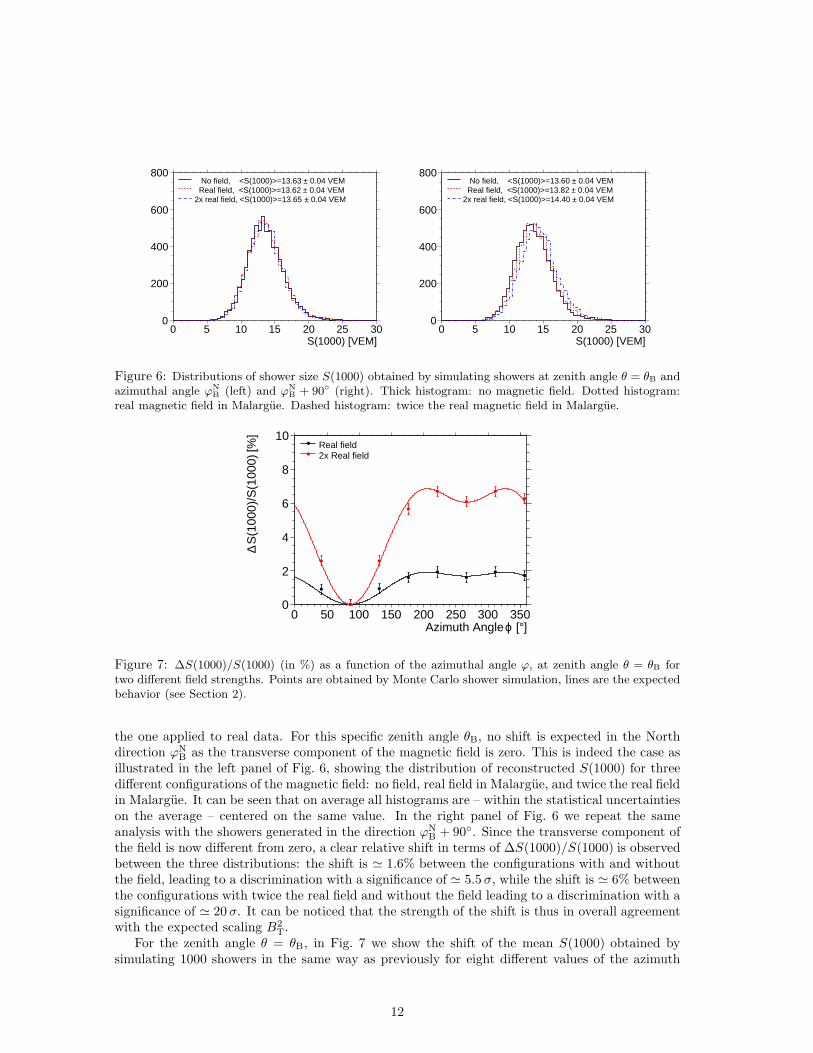
Figure 6: Distributions of shower size S(1000) obtained by simulating showers at zenith angle θ = θB andazimuthal angle ϕN

B (left) and ϕNB + 90◦ (right). Thick histogram: no magnetic field. Dotted histogram:

real magnetic field in Malargue. Dashed histogram: twice the real magnetic field in Malargue.

]° [ϕ Azimuth Angle 0 50 100 150 200 250 300 350

[%]

S(1

000)

/S(1

000)

∆

0

2

4

6

8

10Real field2x Real field

Figure 7: ∆S(1000)/S(1000) (in %) as a function of the azimuthal angle ϕ, at zenith angle θ = θB fortwo different field strengths. Points are obtained by Monte Carlo shower simulation, lines are the expectedbehavior (see Section 2).

the one applied to real data. For this specific zenith angle θB, no shift is expected in the Northdirection ϕN

B as the transverse component of the magnetic field is zero. This is indeed the case asillustrated in the left panel of Fig. 6, showing the distribution of reconstructed S(1000) for threedifferent configurations of the magnetic field: no field, real field in Malargue, and twice the real fieldin Malargue. It can be seen that on average all histograms are – within the statistical uncertaintieson the average – centered on the same value. In the right panel of Fig. 6 we repeat the sameanalysis with the showers generated in the direction ϕN

B + 90◦. Since the transverse component ofthe field is now different from zero, a clear relative shift in terms of ∆S(1000)/S(1000) is observedbetween the three distributions: the shift is ≃ 1.6% between the configurations with and withoutthe field, leading to a discrimination with a significance of ≃ 5.5 σ, while the shift is ≃ 6% betweenthe configurations with twice the real field and without the field leading to a discrimination with asignificance of ≃ 20 σ. It can be noticed that the strength of the shift is thus in overall agreementwith the expected scaling B2

T.For the zenith angle θ = θB, in Fig. 7 we show the shift of the mean S(1000) obtained by

simulating 1000 showers in the same way as previously for eight different values of the azimuth

12

]° [θ Zenith Angle 0 10 20 30 40 50 60 70

) [%

]θ

G(

0

2

4

6

Figure 8: G(θ) = ∆S(1000)/S(1000)/ sin2(u,b) as a function of the zenith angle θ.

angle. Again, the results are displayed for configurations with the real field (bottom) and with twice

the real field (top). The expected behaviours in terms of ∆S(1000)/S(1000) = G(θB) sin2(u,b)are shown by the continuous curves, where the normalisation factor G is tuned by hand. Clearly,the shape of the curves agrees remarkably well with the Monte Carlo data within the uncertainties.Hence, this study supports the claim that the azimuthal dependence of the shift in S(1000) inducedby the magnetic field is proportional to B2

T(θ, ϕ), in agreement with the expectations provided bygeneral considerations expressed in the previous section on the muonic component of the showers.

The B2T term encompassing the overall azimuthal dependence at each zenith angle, the remain-

ing shift G(θ) = ∆S(1000)/S(1000)/ sin2(u,b) depends on the zenith angle through the altitudedistribution of the muon production, the muon energy distribution, and the weight of the muoniccontribution to the shower size S(1000). Repeating the simulations at different zenith angles, weplot G as a function of the zenith angle in Fig. 8. Due to the increased travel lengths of the muonsand due to their larger relative contribution to S(1000) at high zenith angles, the value of G risesrapidly for angles above ≃ 40◦. The superimposed curve is an empirical fit, allowing us to get thefollowing parametrisation of the shower size distortions induced by the geomagnetic field,

∆S(1000)

S(1000)(θ, ϕ) = 4.2 · 10−3 cos−2.8 θ sin2(u,b). (7)

4.2 From shower size to energy

At the Pierre Auger Observatory, the shower size S(1000) is converted into energy E using a two-step procedure [11]. First, the evolution of S(1000) with zenith angle arising from the attenuationof the shower with increasing atmospheric thickness is quantified by applying the Constant Inten-

sity Cut (CIC) method that is based on the (at least approximate) isotropy of incoming cosmicrays. The CIC relates relates S(1000) in vertical and inclined showers through a line of equalintensity in spectra at different zenith angles. This allows us to correct the value of S(1000) forattenuation by computing its value had the shower arrived from a fixed zenith angle, here 38 de-grees (corresponding to the median of the angular distribution of events for energies greater than3 EeV). This zenith angle independent estimator S38 is defined as S38 = S(1000)/CIC(θ). Thecalibration of S38 with energy E is then achieved using a relation of the form E = ASB

38, whereA = 1.49 ± 0.06(stat)±0.12(syst) and B = 1.08 ± 0.01(stat)±0.04(syst) were estimated from thecorrelation between S38 and E in a subset of high quality ”hybrid events” measured simultaneouslyby the surface detector (SD) and the fluorescence detector (FD) [11]. In such a sample, S38 and E

13

]° [δ Declination -80 -60 -40 -20 0 20

[%]

N/N∆

-4

-2

0

2

°=60maxθ°=50maxθ

Figure 9: Relative differences ∆N/N as a function of the declination, for 2 different values of θmax.

are independently measured, with S38 from the SD and E from the FD.This two-step procedure has an important consequence on the implementation of the energy

corrections for the geomagnetic effects. The CIC curve is constructed assuming that the showersize estimator S(1000) does not depend on the azimuthal angle. The induced azimuthal variationof S(1000) due to the geomagnetic effect is thus averaged while the zenith angle dependence of thegeomagnetic effects is absorbed when the CIC is implemented. To illustrate this in a simplifiedway, consider the case in which the magnetic field were directed along the zenith direction (i.e. inthe case of a virtual Observatory located at the Southern magnetic pole) so that the transversecomponent of the magnetic field would not depend on the azimuthal direction of any incomingshower. Then the shift in S(1000) would depend only on the zenith angle in such a way that theConstant Intensity Cut method would by construction absorb the shift induced by G(θ) into theempirical CIC(θ) curve, while the empirical relationship E = ASB

38 would calibrate S38 into energywith no need for any additional corrections.

This leads us to implement the energy corrections for geomagnetic effects, relating the energyE0 reconstructed ignoring the geomagnetic effects to the corrected energy E by

E =E0

(1 + ∆(θ, ϕ))B, (8)

with

∆(θ, ϕ) = G(θ)

[sin2(u,b) −

⟨sin2(u,b)

⟩ϕ

](9)

where 〈·〉ϕ denotes the average over ϕ and where B is one of the parameters used in the S38 toE conversion described above. This expression implies that energies are under-estimated preferen-tially for showers coming from the northern directions of the array, while they are over-estimated

for showers coming from the southern directions, the size of the effect increasing with the zenithangle.

5 Consequences for large scale anisotropy searches

5.1 Impact on the estimated event rate

To provide an illustration of the impact of the energy corrections for geomagnetic effects, wecalculate here, as a function of declination δ, the deviation of the event rate N0(δ), measured if we

14

were not to implement the corrections of the energy estimator by Eq. (8), to the event rate N(δ)expected from an isotropic background distribution.

The “canonical exposure” [17] holds for a full-time operation of the surface detector array abovethe energy at which the detection efficiency is saturated over the considered zenith range. In sucha case, the directional detection efficiency is simply proportional to cos θ,

ω(θ) ∝ cos(θ)H(θ − θmax) (10)

where H is the Heaviside function and θmax is the maximal zenith angle considered. The zenithangle is related to the declination δ and the right ascension α through

cos θ = sin ℓsite sin δ + cos ℓsite cos δ cosα (11)

where ℓsite is the Earth’s latitude of the Observatory. The event rate at a given declination δ andabove an energy threshold Eth is obtained by integrating in energy and right ascension α,

N(δ) ∝∫ ∞

Eth

dE

∫ 2π

0

dαω(θ)dN(θ, ϕ,E)

dE(12)

Note that at lower energies this integral acquires an additional energy and angle dependent detec-tion efficiency term ǫ(E, θ, φ). Hereafter we assume that the cosmic ray spectrum is a power law,i.e. dN/dE ∝ E−γ . From Eq. (8) it follows that if the effect of the geomagnetic field were notaccounted for, the measured energy spectrum would have a directional modulation given by

dN

dE0∝ [1 + ∆(θ, ϕ)]

B(γ−1)E−γ

0 . (13)

This leads to the following measured event rate above a given uncorrected energy Eth,

N0(δ) ∝∫ ∞

Eth

dE0

∫ 2π

0

dαH(cos θ − cos θmax) cos θ [1 + ∆(θ, ϕ)]B(γ−1)

E−γ0 , (14)

where ϕ is related to α and δ through

tanϕ =sin δ cos ℓsite − cos δ cosα sin ℓsite

cos δ sinα. (15)

The event rate N0(δ) as a function of declination is then calculated using Eq. (13) in Eq. (12).The relative difference ∆N/N is shown in Fig. 9 as a function of the declination, with spectralindex γ = 2.7. The energy over-estimation (under-estimation) of events coming preferentially fromthe Southern (Northern) azimuthal directions, as described in Eq. (8), leads to an effective excess(deficit) of the event rate for δ . −20◦ (δ & −20◦), with an amplitude of ≃ 2% when consideringθmax = 60◦. It is worth noting that this amplitude is reduced to within 1% when consideringθmax = 50◦, as shown by the dotted line.

5.2 Impact on dipolar modulation searches

The pattern displayed in Fig. 9 roughly imitates a dipole with an amplitude at the percent level.To evaluate precisely the impact of this pattern on the assessment of a dipole moment in thereconstructed arrival directions and to probe the statistics needed for the sensitivity to such aspurious pattern, we apply the multipolar reconstruction adapted to the case of a partial skycoverage [18] to mock data sets by limiting the maximum bound of the expansion Lmax to 1 (puredipolar reconstruction). Since the distortions are axisymmetric around the axis defined by theNorth and South celestial poles, only the multipolar coefficient related to this particular axis is

15

Amplitude0 0.01 0.02 0.03 0.04 0.05 0.06

0

50

100

150

200N=300,000N=32,000

]°Declination [-80 -60 -40 -20 0 20 40 60 80

0

20

40

60

80

100N=32,000

Figure 10: Dipolar reconstruction of arrival directions of mock data sets with event rates distorted by thegeomagnetic effects. Left: distributions of amplitudes. Right: distributions of declinations. The smoothlines give the expected distribution in the case of isotropy.

expected to be affected (here: a10). Consequently, this particular coefficient has impacts on boththe amplitude of the reconstructed dipole and its direction with respect to the axis defined by theNorth and South celestial poles (the technical details of relating the estimation of the multipolarcoefficients to the spherical coordinates of a dipole are given in the Appendix).

To simulate the directional distortions induced by Eq. (8), each mock data set is drawn fromthe event rate N0(δ) corresponding to the uncorrected energies, and is reconstructed using thecanonical exposure in Eq. (10). The results of this procedure applied to 1000 samples are shownin Fig. 10. In the left panel, the distribution of the reconstructed amplitudes r using N = 300 000events is shown by the dotted histogram. It clearly deviates from the expected isotropic distributiondisplayed as the dotted curve which corresponds to (see Appendix)

pR(r) =r

σ√σ2z − σ2

erfi

(√σ2z − σ2

σσz

r√2

)exp

(− r2

2σ2

), (16)

where erfi(z) = erf(iz)/i, and where the width parameters σ and σz can be calculated fromthe exposure function [18]. With the particular exposure function used here, it turns out thatσ ≃ 1.02

√3/N and σz ≃ 1.59

√3/N . This allows us to estimate the spurious dipolar amplitude4

to be of the order of the mean of the dotted histogram, about ≃ 1.9%. Consequently, we canestimate that the spurious effect becomes predominant as soon as the mean noise amplitude 〈r〉deduced from Eq. (16) is of the order of 1.9%,

〈r〉 =

√2

π

(σz +

σ2arctanh(√

1 − σ2/σ2z)√

σ2z − σ2

)≃ 1.9%. (17)

This translates into the condition N ≃ 32 000 (solid histogram). Using such a number of events,the bias induced on the amplitude reconstruction is illustrated in the same graph by the longertail of the full histogram with respect to the expected one, and is even more evident in the rightpanel of Fig. 10, showing the distribution of the reconstructed declination direction of the dipolewhich already deviates to a large extent from the expected distribution.

4Due to the partial sky exposure considered here, the estimate of the dipolar amplitude is biased by the highermultipolar orders needed to fully describe ∆N/N shown in Fig. 10 [18]. The aim of this calculation is only toprovide a quantitative illustration of the spurious measurement which would be performed due to the geomagneticeffects when reconstructing a pure dipolar pattern.

16

]° [δ Declination -80 -60 -40 -20 0 20

N/N

[%]

∆

-4

-2

0

2

protons, QGSJET01, 5 EeViron, QGSJET01, 5 EeVprotons, QGSJET01, 50 EeVprotons, QGSJETII, 5EeV

µprotons, QGSJET01, 5 EeV, 2xN

Figure 11: Relative differences ∆N/N as a function of the declination, for different primary masses,different primary energies, different hadronic models and for increased number of muons in showers.

6 Systematic uncertainties

The parametrisation of G(θ) in Eq. (7) was obtained by means of simulations of proton showersat a fixed energy. The height of the first interaction influences the production altitude of muonsdetected at 1000 m from the shower core at the ground level. Moreover, as muons are produced atthe end of the hadronic cascade, when the energy of the charged mesons is diminished so much thattheir decay length becomes smaller than their interaction length (which is inversely proportionalto the air density), the energy distribution of muons is also affected by the height of the firstinteraction. Because the air density is lower in the upper atmosphere, this mechanism results inan increase of the energy of muons. The muonic contribution to S(1000) depends also on both theprimary mass and primary energy. For all these reasons, the parametrisation of G(θ) is expectedto depend on both the primary mass and primary energy.

To probe these influences, we repeat the same chain of end-to-end simulations using protonshowers at energies of 50 EeV and iron showers at 5 EeV. Results in terms of the distortions ofthe observed event rate N(δ) are shown in Fig. 11. We also display in the same graph the resultsobtained using the hadronic interaction model QGSJETII [19]. The differences with respect to thereference model are small, so that the consequences on large scale anisotropy searches presentedin Section 5 remain unchanged within the statistics available at the Pierre Auger Observatory.

In addition, there are discrepancies in the hadronic interaction model predictions regardingthe number of muons in shower simulations and what is found in our data [20]. Higher number ofmuons influences the weight of the muonic contribution to S(1000). The consequences of increasingthe number of muons by a factor of 2 on the distortions of the observed event rate are also shownin Fig. 11. As the muonic contribution to S(1000) is already large at high zenith angles in thereference model, this increase of the number of muons does not lead to large differences.

7 Conclusion

In this work, we have identified and quantified a systematic uncertainty affecting the energy deter-mination of cosmic rays detected by the surface detector array of the Pierre Auger Observatory.This systematic uncertainty, induced by the influence of the geomagnetic field on the shower devel-opment, has a strength which depends on both the zenith and the azimuthal angles. Consequently,we have shown that it induces distortions of the estimated cosmic ray event rate at a given energy

17

at the percent level in both the azimuthal and the declination distributions, the latter of whichmimics an almost dipolar pattern.

We have also shown that the induced distortions are already at the level of the statisticaluncertainties for a number of events N ≃ 32 000 (we note that the full Auger surface detectorarray collects about 6500 events per year with energies above 3 EeV). Accounting for these effectsis thus essential with regard to the correct interpretation of large scale anisotropy measurementstaking explicitly profit from the declination distribution.

Acknowledgements

The successful installation, commissioning, and operation of the Pierre Auger Observatory wouldnot have been possible without the strong commitment and effort from the technical and admin-istrative staff in Malargue.

We are very grateful to the following agencies and organizations for financial support: ComisionNacional de Energıa Atomica, Fundacion Antorchas, Gobierno De La Provincia de Mendoza, Mu-nicipalidad de Malargue, NDM Holdings and Valle Las Lenas, in gratitude for their continuingcooperation over land access, Argentina; the Australian Research Council; Conselho Nacional deDesenvolvimento Cientıfico e Tecnologico (CNPq), Financiadora de Estudos e Projetos (FINEP),Fundacao de Amparo a Pesquisa do Estado de Rio de Janeiro (FAPERJ), Fundacao de Am-paro a Pesquisa do Estado de Sao Paulo (FAPESP), Ministerio de Ciencia e Tecnologia (MCT),Brazil; AVCR AV0Z10100502 and AV0Z10100522, GAAV KJB100100904, MSMT-CR LA08016,LC527, 1M06002, and MSM0021620859, Czech Republic; Centre de Calcul IN2P3/CNRS, Cen-tre National de la Recherche Scientifique (CNRS), Conseil Regional Ile-de-France, DepartementPhysique Nucleaire et Corpusculaire (PNC-IN2P3/CNRS), Departement Sciences de l’Univers(SDU-INSU/CNRS), France; Bundesministerium fur Bildung und Forschung (BMBF), DeutscheForschungsgemeinschaft (DFG), Finanzministerium Baden-Wurttemberg, Helmholtz-GemeinschaftDeutscher Forschungszentren (HGF), Ministerium fur Wissenschaft und Forschung, Nordrhein-Westfalen, Ministerium fur Wissenschaft, Forschung und Kunst, Baden-Wurttemberg, Germany;Istituto Nazionale di Fisica Nucleare (INFN), Ministero dell’Istruzione, dell’Universita e dellaRicerca (MIUR), Italy; Consejo Nacional de Ciencia y Tecnologıa (CONACYT), Mexico; Min-isterie van Onderwijs, Cultuur en Wetenschap, Nederlandse Organisatie voor WetenschappelijkOnderzoek (NWO), Stichting voor Fundamenteel Onderzoek der Materie (FOM), Netherlands;Ministry of Science and Higher Education, Grant Nos. N N202 200239 and N N202 207238,Poland; Fundacao para a Ciencia e a Tecnologia, Portugal; Ministry for Higher Education, Sci-ence, and Technology, Slovenian Research Agency, Slovenia; Comunidad de Madrid, Consejerıa deEducacion de la Comunidad de Castilla La Mancha, FEDER funds, Ministerio de Ciencia e In-novacion and Consolider-Ingenio 2010 (CPAN), Xunta de Galicia, Spain; Science and TechnologyFacilities Council, United Kingdom; Department of Energy, Contract Nos. DE-AC02-07CH11359,DE-FR02-04ER41300, National Science Foundation, Grant No. 0450696, The Grainger Founda-tion USA; ALFA-EC / HELEN, European Union 6th Framework Program, Grant No. MEIF-CT-2005-025057, European Union 7th Framework Program, Grant No. PIEF-GA-2008-220240, andUNESCO.

Appendix

The p.d.f. of the first harmonic amplitude for a data set of N points drawn at random over acircle is known to be the Rayleigh distribution. In this appendix, we generalise this distributionto the case of N points being drawn at random on the sphere over the exposure ω(δ) of thePierre Auger Observatory. Assuming the underlying arrival direction distribution to be of the

18

form Φ(α, δ) = Φ0(1 +D ·u), the components of the dipolar vector D are related to the multipolarcoefficients through

Dx =√

3a11a00

, Dy =√

3a1−1

a00, Dz =

√3a10a00

. (18)

Denoting by x, y, z the estimates of Dx, Dy, Dz, the joint p.d.f. pX,Y,Z(x, y, z) can be factorised inthe limit of large number of events in terms of three centered Gaussian distributions N(0, σ),

pX,Y,Z(x, y, z) = pX(x)pY (y)pZ(z) = N(0, σx)N(0, σy)N(0, σz), (19)

where the standard deviation parameters can be calculated from the exposure function [18]. Withthe particular exposure function used here, it turns out that numerical integrations lead to σ ≃1.02

√3/N and σz ≃ 1.59

√3/N . The joint p.d.f. pR,∆,A(r, δ, α) expressing the dipole components

in spherical coordinates is obtained from Eq. (19) by performing the Jacobian transformation

pR,∆,A(r, δ, α) =

∣∣∣∣∂(x, y, z)

∂(r, δ, α)

∣∣∣∣ pX,Y,Z(x(r, δ, α), y(r, δ, α), z(r, δ, α))

=r2 cos δ

(2π)3/2σ2σzexp

[−r

2 cos2 δ

2σ2− r2 sin2 δ

2σ2z

]. (20)

From this joint p.d.f., the p.d.f. of the dipole amplitude (declination) is finally obtained bymarginalising over the other variables, yielding

pR(r) =r

σ√σ2z − σ2

erfi

(√σ2z − σ2

σσz

r√2

)exp

(− r2

2σ2

),

p∆(δ) =σσ2

z

2

cos δ

(σ2z cos2 δ + σ2 sin2 δ)3/2

. (21)

Finally, one can derive from pR quantities of interest, such as the expected mean noise 〈r〉, theRMS σr and the probability of obtaining an amplitude greater than r:

〈r〉 =

√2

π

(σz +

σ2arctanh(√

1 − σ2/σ2z)√

σ2z − σ2

), (22)

σr =

√2σ2 + σ2

z − 〈r〉2, (23)

Prob(> r) = erfc

(r√2σz

)+

σ√σ2z − σ2

erfi

(√σ2z − σ2

√2σσz

r

)exp

(− r2

2σ2

), (24)

which are the equivalent to the well known Rayleigh formulas 〈r〉 =√π/N, σr =

√(4 − π)/N and

Prob(> r) = exp(−Nr2/4) when dealing with N points drawn at random over a circle [21].

Acknowledgments

References

[1] D. M. Edge et al., J. Phys. A 6 (1973) 1612.

[2] M. Ave, R. A. Vazquez, and E. Zas, Astropart. Phys. 14 (2000) 91.

[3] M. Ave et al., Astropart. Phys. 14 (2000) 109.

19

[4] H. Dembinski et al., Astropart. Phys. 34 (2010) 128.

[5] K. Greisen, Ann. Rev. Nuc. Sci. 10 (1960) 63.

[6] K. Kamata and J. Nishimura, Prog. Theor. Phys. 6 (1958) 93.

[7] A. Ivanov et al., JETP Letters 69 (1999) 288.

[8] P. Bernardini et al. for the ARGO-YBJ Collaboration, Proceedings of the 32nd ICRC, Beijing,China, arXiv:1110.0670; H.H. He et al., Proceedings of the 29th ICRC, Pune, India

[9] J. Abraham et al. [Pierre Auger Collaboration], Nucl. Instrum. Meth. A 523 (2004) 50.

[10] J. Abraham et al. [Pierre Auger Collaboration], Nucl. Instr. and Meth. A 613 (2010) 29-39.

[11] J. Abraham et al. [Pierre Auger Collaboration], Phys. Rev. Lett. 101 (2008) 061101.

[12] National Geography Data Center, http://www.ngdc.noaa.gov/seg/geomag/geomag.shtml,2007.

[13] X. Bertou, et al., Pierre Auger Collaboration, Nucl. Instr. and Meth. A 568 (2006) 839.

[14] S.J. Sciutto, Proceedings of the 27th ICRC, Hamburg, Germany, arXiv:astro-ph/0106044v1.

[15] N.N. Kalmykov and S.S. Ostapchenko, Yad. Fiz. 56 (1993) 105; N.N. Kalmykov, S.S.Ostapchenko, and A.I. Pavlov, Nucl. Phys. B Proc. Suppl. 52B (1997) 17.

[16] D. Heck et al., Report FZKA 6019, Karlsruhe, Germany, 1998.

[17] P. Sommers, Astropart. Phys. 14 (2001) 271.

[18] P. Billoir and O. Deligny, JCAP 02 (2008) 009.

[19] S.S. Ostapchenko, Nucl. Phys. B Proc. Suppl. 151 (2006) 147-150.

[20] R. Engel for the Pierre Auger collaboration, Proceedings of the 30th ICRC, Merida, Mexico,arXiv:0706.1921.

[21] J. Linsley, Phys. Rev. Lett. 34 (1975) 1530.

20