The effect of

river red gum decline on woodland birds in the Macquarie MarshesAlice Blackwood, Richard Kingsford, Lucy Nairn, Tom Rayner

Australian Wetlands & Rivers CentreSchool of Biological, Environmental and Earth Sciences

University of New South Wales

May 2010

Acknowledgements

We wish to acknowledge the Wailwan people, traditional owners of the Macquarie

Marshes, and the Eora people, traditional owners of UNSW and Sydney.

This project was made possible by the generous funding of the NSW Department of

Environment, Climate Change and Water, the Australian Geographic Society, the Wildlife

Preservation Society of Australia and the Birds Australia (Stewart Lesley Bird Research

Award).

Thank you to everyone at the Wetlands and Rivers Centre, in particular to Kim Jenkins, Ben

Wolfenden and John Porter for statistics advice and Shiquan Ren for providing flood history

data.

We would like to thank all our fieldwork volunteers: Julia Blackwood, Jenny Spencer, Kathy

Wilk, Heather Hartford, Tessa Dowdell, Fiona Johnson, Sujata Allan, Jo Ocock, Chris

Marshall, Jim Blackwood, Misti de Montfort.

Thanks also to Ray and Sue Jones for sharing their wisdom, Steve Tucker for his general

assistance, Frank Hemmings, Mailie Gall, and Ross McMurtrie for their generous help with

equipment and software.

2

Table of Contents 1 Executive Summary ......................................................................................................................... 3

2 Introduction .................................................................................................................................... 5

3 Study area ....................................................................................................................................... 8

4 Methodology ................................................................................................................................... 9

4.1 Health categorisation .............................................................................................................. 9

4.2 Site selection ........................................................................................................................... 9

4.3 Woodland Bird surveys ......................................................................................................... 13

4.4 Vegetation ............................................................................................................................. 14

4.5 Guilds .................................................................................................................................... 18

4.6 Statistical analyses ................................................................................................................ 18

5 Results ........................................................................................................................................... 23

5.1 Birds ...................................................................................................................................... 23

5.2 Vegetation ............................................................................................................................. 34

6 Discussion ...................................................................................................................................... 47

7 References .................................................................................................................................... 52

Appendix 1: Bird species list- Macquarie Marshes, May-August 2009 ................................................. 59

Appendix 2: Understorey vegetation species list ................................................................................. 64

Appendix 3: Site locations ..................................................................................................................... 65

3

1 Executive Summary The state of woodland birds in Australia is well known with long-term declines attributed to

loss of habitat, mainly through land clearing. Woodland birds are generally passerines (e.g.

honeyeaters and robins) but also include parrots, pigeons, cuckoos and other bird. The

relationship of woodland birds to rivers is not so well known nor is the effect of river

regulation on this group. Yet many woodland birds depend on the rivers and wetlands

because these are often the more productive areas in an otherwise dry environment. Even

when wetlands are dry, they often have larger and more dense trees which provide good

habitat for woodland birds. We found that woodland bird communities changed

substantially depending on the health of floodplain trees. Healthier floodplain communities

had higher abundances of foliage specialist birds, reflecting greater canopy cover, while

floodplain communities in poor health had high abundances of birds that are typical of open

agricultural areas (eg. Crested pigeon, jacky winter), and a community similar to surrounding

terrestrial areas.The number of species and their abundance remained similar across health

categories but the community composition changed.

Regulation of rivers worldwide has reduced the ecological resilience and biodiversity of

riparian and floodplain ecosystems and their dependent biota. Most knowledge of this is of

the effects on aquatic organisms, but some terrestrial animals, such as woodland birds, may

also be dependent on flows. We investigated differences in the woodland bird community

among stands of river red gums in the Macquarie Marshes in three health categories: poor,

intermediate and good. We created a map of river red gum health, categorising stand health

as good, intermediate or poor from aerial photos, for selection of 10 sites for woodland bird

surveys in each health category. We surveyed woodland birds at each site in autumn and

spring over a two-hectare area for 20 minutes, recording species, abundance and

microhabitat preferences. At each site, we surveyed vegetation: species, structure,

abundance and health of understorey and trees. We also surveyed birds at three terrestrial

sites, further out on the floodplain.

There was no difference in the abundance of large (50 – 100 cm and >100 cm diameter at

breast height) trees among the tree health categories (F2,27=2.056, p=0.13 and F=1.979,

p=0.14 respectively), indicating that sites were once in similar condition. Abundance of small

trees (2-10 cm, usually young) was significantly different among health categories

(F2,27=5.88, p=0.004), with high abundance at good sites reflecting more favourable flooding

conditions in recent years. There was no difference in abundance of hollows among the

three health categories (F2,27=1.94, p=0.16), but the number of fruiting river red gums did

differ, favouring healthier trees (F2,27=6.105, p<0.001).

The composition of the woodland bird community was significantly different among health

categories (PERMANOVA PseudoF=2.1538, P(perm)=0.001) even though there was no

difference in species richness, overall abundance or diversity. Furthermore, the bird

communities of the three terrestrial sites were similar to those of the poor and intermediate

4

sites, indicating a ‘terrestrialisation’ of the system. Many of the species that were more

abundant at poor sites, such as rufous songlark and crested pigeon, are typical of open,

agricultural areas. The patterns of the bird community were significantly correlated with

changes in tree health and habitat structure (BEST analysis, Rho=0.405, p=0.01), with

patterns best explained by five variables: canopy density, bare ground, shrub cover,

percentage of dead branches and large coarse-woody debris. Good sites were typified by

trees with dense canopy, more leaf litter and low green herbaceous understorey, while poor

sites had trees with thin or absent canopy, more bare ground and tall, dry, shrubby

understorey.

Foliage specialists, such as striated pardalote, weebill, grey fantail and crested shrike-tit,

were most affected by river red gum decline, with declining canopy cover causing decreased

abundances. Live branch specialists, such as galah and white-breasted cuckoo-shrike were

also most abundant at healthy sites. They were replaced by dead tree specialists, such as

hooded robin, rufous songlark, southern whiteface and crested pigeon, which were more

abundant at sites in poor health. Generalist species, such as magpie lark, willie wagtail and

jacky winter, were most resilient to decline, while understorey specialists (fairy-wrens) were

most abundant at sites of intermediate health, probably due to the combination of a

shrubby understorey with some live trees and herb cover. These changes in the bird

community and vegetation were linked with flood history, reflecting long term degradation.

Habitat quality of poor sites will probably degrade further, as dead trees fall over, reducing

the availability of perches and nesting hollows.

The river red gum forests and woodlands of the Macquarie Marshes Northern Nature

Reserve were severely degraded. At poor sites, an average of 58% of tree basal area was

dead, in comparison to 20% at intermediate and poor sites. Cunningham scores of sites,

which are a composite of crown vigour, canopy density and percentage live basal area,

indicated that no sites were in truly good condition; instead, 17 were classified as ‘poor’,

eight as ‘degraded’ and five as ‘severely degraded’. The dominance of the aggressive white-

plumed honeyeater is a further evidence for this degradation. As river red gum health has

declined, the understorey has changed significantly, with the dominance of dense terrestrial

chenopod shrub species such as Sclerolaena sp., replacing aquatic plant species and herbs.

The Macquarie Marshes are losing their unique ecological value and this is not only

reflected in declining aquatic biota but also a changing woodland bird community. The

woodland bird community is increasingly reflecting one of terrestrial habitats, rather than

an aquatic ecosystem. Reversing this decline requires increases in environmental flows,

currently supported by major government programs.

5

2 Introduction Rivers not only drive aquatic ecosystems, supporting their dependent organisms and

processes but also supply resources for some terrestrial organisms (Baxter et al. 2005;

Kingsford et al. 2006; Likens and Bormann 1974). Resources that move across permeable

boundaries from one system to another in this way are known as ‘subsidies’, ‘donations’ or

‘allochthonous inputs’ (Ballinger and Lake 2006) and may benefit organisms directly or

indirectly (Polis et al. 1997). These resources support higher densities of consumers than

would be possible in purely terrestrial systems, augment productivity (Bastow et al. 2002;

Ballinger and Lake 2006) and increase food web stability (Huxel and McCann 1998). For

example, flooding enhances the survival and dispersal of the yellow-footed antechinus

(Antechinus flavipes), a terrestrial marsupial (Lada et al. 2007). Even passerines at high

densities in Alaskan forests are supported by salmon-spawning streams (Gende and Willson

2001). Nutrients and detritus carried by floodwaters, as well as the water, usually boost

primary productivity of terrestrial systems (Polis et al. 1997). Aquatic insects can be an

important food source for terrestrial consumers (Gray 1993; Ballinger and Lake 2006; Chan

et al. 2008). For example aquatic invertebrates can make up over 25 % of the annual total

energy budget of forest birds in Japan (Nakano and Murakami 2001). Higher densities of

woodland birds, especially insectivores are common in riparian areas, compared to nearby

areas (Stauffer and Best 1980; Ford et al. 2001; Gende and Willson 2001; Palmer and

Bennett 2006).

As our understanding of the importance of river systems for terrestrial species increases,

there is accumulating evidence that freshwater ecosystems are declining in function and

resilience around the world. Over half of the world’s large river systems are now affected by

dams, which are capable of storing about 15% of the global total annual river runoff (Nilsson

et al. 2005). Worldwide impoundment of water has been so extensive that it has even

affected sea levels (Sahagian 2000) and minutely changed the Earth’s axis and increased the

speed of its rotation (Chao 1995). Riverine floodplains, among the most biologically

productive and diverse global ecosystems, are also among the most threatened (Lemly et al.

2000; Klement and Jack 2002). Increasing human populations are driving demand for

irrigated agriculture, power generation and water for urban and industrial use, substantially

increasing numbers of dams, water diversions, weirs, levees and off-river storages (Lemly et

al. 2000; Nilsson et al. 2005). Such river regulation has dramatically changed the flow of

rivers across the land, altering the frequency, duration and extent of floodplain inundation

Other threats are often additive: chemical contamination (Lemly et al. 2000), habitat

degradation, species invasions and climate change (Allan and Flecker 1993). A global

temperature rise of 3-4°C is predicted to eliminate 85% of the world’s wetlands (UNEP-

WCMC 2001).

In Australia, the most heavily regulated system is the Murray-Darling Basin (MDB) (Kingsford

2000), the nation’s most economically important river basin. It yields $15 billion a year in

agricultural products, accounts for more than half of Australia’s water consumption (ABS

6

2008), and contains some of the longest river systems in the world (Walker 2006). Before

regulation, the rivers of the MDB were characterised by high variability, slow flows and

gently sloping land (Reid and Brooks 2000). There are now more than twenty large

headwater dams and 6000 regulating weirs, and the discharge of rivers within the basin has

been reduced by between 20 and 81 % (Thoms 2006). More than 94 % of the flow capacity

of the system can be stored in the 30 largest dams (Walker 2006). Seasonality of flows in the

south has changed from predominantly winter and spring to summer flows, and the

frequency of small and medium sized floods has decreased dramatically (Maheshwari et al.

1995).

Such dramatic changes to flows have affected the ecological integrity of aquatic systems.

Loss of flooding reduces macroinvertebrate biomass (Boulton and Lloyd 1992) and species

richness (Jenkins and Boulton 2007, Sabella 2009) on floodplains. Fish have been affected,

with dams and other man-made structures creating barriers for fish passage, changing flows

and altering aquatic habitat (Gehrke et al. 1995; Kingsford et al. 2006; Rayner et al. 2009).

These changes to food sources along with altered habitat and breeding conditions have had

significant impacts upon waterbird distribution, diversity and breeding (Briggs et al. 1997;

Kingsford and Johnson 1998; Kingsford and Auld 2003; Kingsford et al. 2004; Kingsford and

Thomas 2004). In addition, river regulation has changed the distribution, diversity and

composition of vegetation communities (Shafroth et al. 2002; Brock et al. 2006; Richardson

et al. 2007, Sabella 2009). Perennial flood dependent eucalypts, such as river red gums

Eucalyptus camaldulensis have been particularly affected by major changes to river flows

(Bren 1988; Jansen and Robertson 2001b; MDBC 2003; Cunningham et al. 2007a;

Cunningham et al. 2007b)

River red gums are the most widely distributed eucalypt in Australia (Keith 2004;

Cunningham et al. 2007a) and grow in extensive monospecific stands or as lines of trees

along river banks in riparian areas (Di Stefano 2002). Across large areas of the MDB river red

gums are exhibiting deteriorating health, canopy dieback, insect damage, minimal

regeneration, increased parasitism, and eventually tree death (MDBC 2003; Cunningham et

al. 2007a). Some trees have also been killed by prolonged inundation (Briggs et al. 1997; Di

Stefano 2002). Lack of flooding can almost halve the relative growth rate of river red gums

and decrease average leaf area (Cunningham et al. 2007a). The vegetation understorey may

also change with reduced flooding frequency (Bren and Gibbs 1986; Bren 1988; Nairn and

Kingsford, unpubl. data).

Such major changes to floodplains and flooding regimes alter productivity at the landscape

level, with effects cascading through the food web (Bunn et al. 2006). River red gums play

an important role in nutrient cycling between floodplains and rivers (Cunningham et al.

2007b). They also provide habitat and food for a range of terrestrial species, including a

diverse suite of woodland birds (Di Stefano 2002). This includes the vulnerable superb

parrot, Polytelis swainsonii, which requires large healthy river red gums for breeding

7

(Webster in Di Stefano 2002). Woodland birds, or bush-birds, use river floodplains and

riparian areas for habitat, foraging, breeding, and watering (Johnson et al. 2007). When

compared with other habitat types in the Murray catchment, river red gum forest had the

highest total abundance and species richness of woodland birds (Oliver and Parker 2006).

The Macquarie Marshes are in decline, as a result of a long history of river regulation

(Kingsford and Thomas 2004). River red gum decline is one of the many ways this decline

has manifested. Water diversions support a $400 million agricultural industry, of which

cotton is the dominant irrigation enterprise (DECC 2009). Burrendong Dam, the major

storage structure in the system, was constructed in 1967. Since that time, the frequency,

duration and extent of floods have decreased significantly, while some channels are now

subject to constant low flows. This has significantly impacted upon the ecology of the

Macquarie Marshes. Much of the semi-permanent wetland mapped in the early 1990s no

longer supports wetland vegetation (DECC 2009), and waterbirds have been adversely

affected (Kingsford and Thomas 1995). In addition to river regulation, rainfall and flows have

been extremely low over the past decade. Little information exists about the relationship

between vegetation and woodland birds in the Macquarie Marshes (DECC 2009).

The aim of this study was to assess the impact of river red gum decline in the Macquarie

Marshes on the woodland bird community. Given the importance of river red gum to

woodland birds, we predicted that river red gum forests in poor ecological health would

support a different bird community to river red gums in good ecological health. We

investigated the extent and nature of these changes, through different measures of the

woodland bird community and river red gum community and related these to changed

flooding regimes.

8

3 Study area The Macquarie Marshes is a large floodplain wetland at the lower end of the Macquarie

River (Figure 1), covering an area of >200 000 ha, about 10% of which is within a Nature

Reserve. The Marshes are listed under the Ramsar Convention as a wetland of international

importance and are also listed by the National Trust of Australia and Australian Heritage

Commission as having conservation importance(DECC 2009). There is a complex system of

branched channels conveying water to a range of wetland types, ranging from lagoons and

semi-permanent marshes to permanent wetlands, providing essential habitat for a large

range of biota (DECC 2009). A total of 76 waterbird species have been recorded in the

Macquarie Marshes, and some of the larger waterbird breeding events in Australia have

been recorded there (DECC 2009). River red gums are an important habitat for a diverse

suite of woodland birds (over 120 species) in the Macquarie Marshes (Appendix 1). Eighteen

of these species are declining (Reid in DECC 2009), and four are listed as vulnerable under

the NSW Threatened Species Conservation Act 1995: the brown treecreeper, diamond

firetail, hooded robin and grey-crowned babbler.

The Macquarie Marshes have a diverse mosaic of vegetation types created by variable flows

and a complex network of channels. These include river red gum woodlands, which are

typically on floodplain clays close to watercourses, with blackbox (Eucalyptus largiflorens)

and coolibah (E. coolabah) further out (Shelly 2005). Other major vegetation communities

include cumbungi (Typha domingensis), water couch (Paspalum distichum), lignum

(Muehlenbeckia florulenta) and common reed (Phragmites australis). The understorey is

variable, from aquatic species, reeds, rushes and sedges in the wetter parts, to grasses and

forbs in dry areas (DECC 2009). River red gums in the Macquarie Marshes cover an area of

40 000 ha (Wilson in DECC 2009), constituting the largest northern area of river red gums

(EPA 1995). Already affected by clearing and ring-barking early in the 20th century (Brander

1987), large areas of river red gums have declined in health recently, due to changes in the

flood regime (Bacon 1994; Nairn 2008). One third of river red gum sites in the northern part

of the Macquarie Marshes have died because of river regulation, abstraction and drought

(Steinfeld and Kingsford 2008). Some of these areas only began to show signs of stress in

2001 (R. Jones, NPW, pers. comm.).

9

4 Methodology

4.1 Health categorisation

This project focused specifically on woodland bird communities in river red gum woodlands

within the Northern Macquarie Marshes Nature Reserve, an area where effects of livestock

grazing would not confound research results. Areas of river red gums were identified from

existing vegetation survey data (Wilson 2008) and then divided into three categories of

condition: poor, intermediate and good. This was achieved by visual assessment of digital

aerial photos of the Northern Nature Reserve (resolution 40 cm; 2006) which had been

rectified and georectified (projection GDA94, MGA zone 55). Visual interpretation was

preferred over automated classification as it allowed for use of texture, shape and pattern

of vegetation (Danby and Hik 2007). We created polygons around areas of river red gums in

similar condition, based on similarities in canopy cover, texture and colour. To classify

health we then generated random points within these polygons, and estimated the

percentage of dead or extremely stressed trees, identified by their lack of canopy, within a

50m circle of each point (Figure 2). Random points (n=100 total) were generated using

Hawth’s Tools (Beyer 2004) in ArcGIS (ESRI 2006). Polygons were classified into one of three

condition categories based on the number of dead or extremely stressed trees at the points

within each polygon: good 0-10%, intermediate 20-70%, poor 80-100 %. The result of this

process was a map of the three categories of river red gum health within the Macquarie

Marshes Northern Nature Reserve (Figure 3). Existing vegetation maps (Wilson 2008) were

checked to ensure tree density was standardised across the three categories.

4.2 Site selection

We randomly selected 33 sites (10 good, 10 intermediate, 13 poor) within the three

categories. We created a 500m buffer around all access roads, within which we used

Hawth’s tools (Beyer 2004) to generate random points in the three health categories. This

buffer ensured accessibility and enabled me to survey woodland birds at three sites each

morning. The unbalanced design (Figure 4) reflected the size and accessibility of the

respective areas. We ensured that the minimum distance between sites was 500m to avoid

pseudoreplication. For comparison we also conducted bird surveys at three terrestrial sites,

located in ‘Ninnia’, part of the Macquarie Marshes nature reserve further out on the

floodplain. Power analysis using means from pilot surveys indicated that 10 sites of each

category would give a power > 0.8 to detect differences in both species richness and overall

abundance.

10

Figure 1 Site map showing the location of the Murray Darling Basin, Macquarie River catchment and Macquarie Marshes (Rayner 2009). The Macquarie Marshes Nature Reserve is shown in grey; this study was based in the northern nature reserve. ‘Ninnia’ is the smaller nature reserve area located to the east.

11

50 m a b

Figure 2 Examples of selected areas (50 m radius) assessed for percentage of dead trees. Figure a has 0 % dead, and so is classified as good, and figure b has 100 % dead or extremely stressed trees, identified by the spider-like forms and shadows of trees with bare branches, and so is classified as poor.

12

Figure 3 Map of the Macquarie Marshes Northern Nature Reserve showing areas of river red gums categorised by health and survey sites

13

4.3 Woodland Bird surveys

Using a repeated-measures design sites were surveyed in late autumn (May-June 2009,) and

early spring (August 2009). These periods were expected to coincide with non-breeding and

breeding periods respectively. Rainfall interrupted the non-breeding survey period, so

surveys were completed in two phases (May 5-10, June 15-19). We resurveyed three sites

surveyed in May to ensure that pooling these two phases was appropriate, and found no

significant difference in the bird community detected between these two phases (ANOSIM

global R=0.407, p=0.2). For logistical reasons, sites near each other were surveyed together,

but to minimise temporal bias, the order of visits was varied between sites and groups of

sites.

Woodland birds were surveyed at each site using the two-hectare search method (Barrett et

al. 2003). This is a standardised method for surveying woodland birds in Australia (eg. Oliver

and Parker 2006; Johnson et al. 2007; Martin and McIntye 2007). To standardise search

effort, we followed a repeatable modified line transect (marked with flags the day before)

through each site, along an inner rectangle, 25 m from the boundary, ensuring that the

entire sample area was covered. Line transects are often preferred over point counts as

they are efficient for data collection, more accurate, less susceptible to bias due to bird

movement, and easier to analyse (Bibby et al. 2000). Although this method may

underestimate the presence of cryptic species (Pyke and Recher 1984), it is effective for

detecting differences in species richness among habitats and broad differences in

community composition (Bibby et al. 2000). All birds heard and seen in a two-hectare site

(100x200m rectangle) during 20 minutes were recorded. Care was taken not to record birds

twice.

To test for differences in detectability, pilot surveys were conducted for one hour at one site

of each health category. Although more species were detected with more time spent at

each site, the rate of detection was similar at all health categories, indicating that

detectability did not differ (Figure 5).

Season (2)

Replication (10-13)

Health (3)

River red gums

Good

n=10

Autumn Spring

Intermediate

n=10

Autumn Spring

Poor

n=10

Autumn Spring

n=3

Autumn

Figure 4 Hierarchical surveying design for woodland bird and understorey surveying showing the two factors Health and Season. There were three health treatments (Good, Intermediate and Poor), and two surveying periods (autumn and spring). Ten sites each were surveyed within each health category. Each site was surveyed once in each survey period, with the exception of three poor sites, which were unable to be surveyed in spring due to time constraints (total n=63)

14

For each woodland bird observed, four variables of habitat use were recorded: 1) position in

the vegetation (on ground, in understorey, or in tree); 2) whether trees occupied were dead

or alive, and 3) position in tree (dead or live branch, trunk or foliage), 4) height of the bird in

occupied tree (0-5 m, 5-10 m, >10 m) and 5) the species of the tree. Bird activity at first

observation (feeding/foraging, perching, calling, preening, darting, flying or other) was also

recorded. Surveys were conducted in a 3 hour window beginning at dawn. Surveys were

only conducted in fine weather and low winds (maximum wind 8.4 km hr-1, measured at

each site) (Bibby et al. 2000). Two surveyors (myself and another) were used in autumn to

maximise sample sites coverage. To minimise inter-observer differences, the two observers

did training surveys in the area (Maron et al. 2005). Additionally, we tested for differences

between the two observers with three independent simultaneous surveys over five minutes,

and found no significant difference.

Figure 5 Species accumulation over time for the three health categories

4.4 Vegetation To investigate relationships between woodland birds and river red gum communities, we

surveyed understory structure and floristics as well as tree health at each site using a system

of small and large quadrats positioned along transects (Figure 5, Table 1). Different

organisms vary over different scales, necessitating the use of quadrats of varying sizes. The

variables measured using the different survey methods are summarised in Table 1.

Understorey was measured using 10 (2x10 m) quadrats spaced evenly along two transects.

The percentage cover of bare ground, leaf litter, and dominant vegetation were recorded.

All vegetation was identified and recorded, except species covering < 5% of each quadrat.

Some plants, such as Chenopodiaceae and Asteraceae were only identified to genus as this

gave sufficient information on plant form and habitat structure. These quadrats were also

0

2

4

6

8

10

12

14

16

18

20

0 20 40 60 80

Cu

mu

lati

ve s

pe

cie

s co

un

t

Time (min)

Good

Int

Poor

15

used to estimate understorey height, the abundance of coarse woody debris (CWD) (5-50

cm, > 50 cm) and river red gum seedlings, an understorey greenness index (1 = mostly dry,

i.e. 0 – 30 % green, 2 = 30 – 70 % green, 3 = 70 – 100 % green) and any flowering or fruiting.

Understorey surveys were conducted in both survey periods in order to investigate seasonal

changes. Another observer was used for 11 sites in autumn and so observer differences

were estimated with independent surveys of two sites in different condition. There was no

difference in understorey composition as assessed by the two observers (ANOSIM global R =

-0.064, p=0.85).

To obtain estimates of percentage live basal area, tree density and demographics, trees

were counted and identified in 10 (20 x 20 m) quadrats evenly spaced along transects

(Figure 5) in each survey site, recording size class by diameter at breast height (DBH): > 100

cm, 50–100 cm, 10-50 cm and 2–10 cm (Jansen and Robertson 2001b). Trees were also

classified as live (with green leaf growth and intact bark) or dead (no green leaves and bark

peeling away) (Cunningham et al. 2007a). Given that trees are long lived and there were no

unusual weather patterns between surveys, these data were only collected in autumn.

To measure the health of trees, ten trees were assessed at each site for nine characteristics:

crown vigour; canopy density (% projective cover; percentage of dead branches; size class

and height class (0-5 m, 5-10 m, 10-20 m, >20m); and the presence or absence of hollows,

mistletoe, flowering and insect damage. Crown vigour was the proportion of potential

crown size, based on existing branches by observing the tree from a distance and using a

visual aid (Figure 7). Along with percentage live basal density and plant area index, crown

vigour is one of the more reliable and objective measures of river red gum health

(Cunningham et al. 2007a). Trees were selected using an adaptation of the ‘zig-zag selection

method’ (Figure 8) (Hnatiuk et al. 2006). As the focus of this study was long-term health

decline, only trees with a DBH greater than ten centimetres were assessed, disregarding

saplings, which may not yet have been fully established (George et al. 2005). These surveys

were also only conducted in autumn.

16

Table 1 Summary of the variables measured using the two different quadrat sizes and individual tree assessments. Ten of each survey method were carried out at each site.

Survey method Variables recorded

2 x 10 m quadrat Percentage cover of understorey components Height of understorey covers Understorey green-ness Number of coarse woody debris (CWD)- small (5-50 cm) and large (> 50 cm) Number of river red gum saplings

20 x 20 m quadrat Number and species of live and dead trees of four different size classes determined by diameter at breast height (DBH): 2 - 10 cm, 10 - 50 cm, 50 – 100 cm, > 100 cm (Jansen and Robertson 2001b)

Individual tree assessment Canopy density Crown vigour Percentage of dead branches Presence of insect damage (> 25 % of leaves) Size (DBH) Height Presence of hollows Presence of mistletoe

20 m

2 m

20 m

10 m

Figure 6. Large quadrats (20x10m) to survey vegetation were spread evenly along the transect and understorey recorded in smaller 2x10m quadrats. The blackened circle represents the tree chosen for health assessment.

17

Figure 7 Visual aid for estimating crown vigour (DSE inSRA 2007).

Figure 8 The zig-zag method for selecting trees for assessment. After assessing one tree, the next must be ahead of and towards or on the other side of the transect (Hnatiuk et al. 2006). In addition for this study, successive trees were spaced at least 40 m apart.

18

4.5 Guilds

To analyse broad differences in community structure, woodland birds were grouped into

guilds (Wilson 1999).Guilds are often used to detect community shifts (Croonquist and

Brooks 1991; Fischer et al. 2007). These may be based on distribution according to

environmental conditions (Beta guilds) or resource type used, within communities (alpha

guilds) (Wilson 1999). For instance, birds may be classified into alpha guilds based upon

their food type and the substrate on which they forage (Fischer et al. 2007). On the other

hand, beta guilds may be formed by measuring certain characters of each species and using

a cluster analysis to form groups of species that occur together or have similar niches

(Wilson 1999). By grouping species into guilds and examining changes in guild structure we

can gain perspective on the functional resilience of communities (Fischer et al. 2007) and

the ecological processes behind community change (Roberts 1987). For the present study,

birds were classified into broad guilds on the basis of habitat use data collected during field

surveys (using cluster analysis, discussed further below).

4.6 Statistical analyses we tested for the effect of health and season on bird species richness, abundance and

diversity (Shannon diversity index, which takes into account relative abundances), and on

abundances of the 10 most common species and all listed threatened species, using a

repeated-measures one-way analysis of variance (ANOVA) (Table 2).Health and season were

both fixed factors with three and two levels respectively, and sites were the replicates. For

understorey variables, which were measured in both seasons, repeated measures ANOVAs

were run (Table 3), with site as a random factor nested within health and quadrats as

replicates. We ran one-way ANOVAs to test for differences in whole-site vegetation

variables between health categories (Table 4) and nested ANOVAs to test variables

measured only in one season but with quadrats as replicates (Table 5).Where there were

significant differences, we ran pairwise comparisons with Tukey’s post hoc tests. All

univariate analyses were run in SYSTAT v11.0. The variables tested under each ANOVA

design are summarised in Table 6.

In order to assess whether the red gum community was once in similar condition at all

categories, abundances of river red gums in the four size classes was tested, pooling live and

dead trees to indicate what the community may have been like in the absence of water

stress. Counts of live and dead trees were still used to calculate percentage live basal area.

The major measure of whole-site health used was the “Cunningham” index, which is a

composite of crown vigour, canopy density and percentage live basal area, each

contributing 0-5 points to produce a maximum health index of fifteen (Cunningham et al.

2007a). These scores are divided by Cunningham et al. into five health classes: good (12.1-

15), declining (9.1-12), poor (6.1-9), degraded (3.1-6) and severely degraded (0.2-3) (not to

be confused with the health categories derived from aerial photo analysis used in this

study).

19

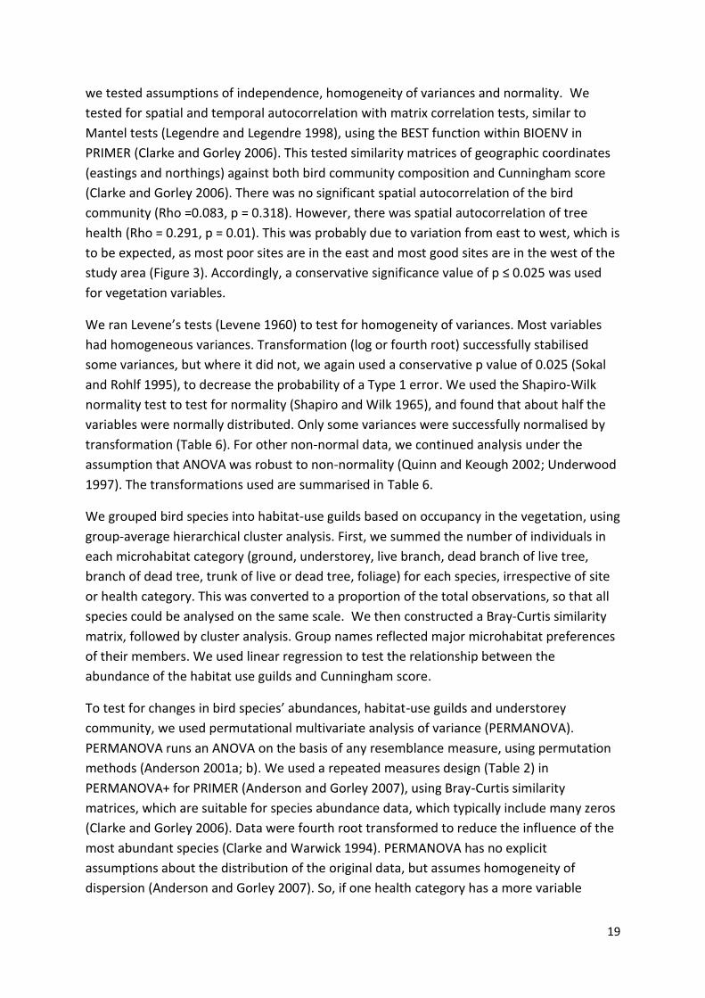
we tested assumptions of independence, homogeneity of variances and normality. We

tested for spatial and temporal autocorrelation with matrix correlation tests, similar to

Mantel tests (Legendre and Legendre 1998), using the BEST function within BIOENV in

PRIMER (Clarke and Gorley 2006). This tested similarity matrices of geographic coordinates

(eastings and northings) against both bird community composition and Cunningham score

(Clarke and Gorley 2006). There was no significant spatial autocorrelation of the bird

community (Rho =0.083, p = 0.318). However, there was spatial autocorrelation of tree

health (Rho = 0.291, p = 0.01). This was probably due to variation from east to west, which is

to be expected, as most poor sites are in the east and most good sites are in the west of the

study area (Figure 3). Accordingly, a conservative significance value of p ≤ 0.025 was used

for vegetation variables.

We ran Levene’s tests (Levene 1960) to test for homogeneity of variances. Most variables

had homogeneous variances. Transformation (log or fourth root) successfully stabilised

some variances, but where it did not, we again used a conservative p value of 0.025 (Sokal

and Rohlf 1995), to decrease the probability of a Type 1 error. We used the Shapiro-Wilk

normality test to test for normality (Shapiro and Wilk 1965), and found that about half the

variables were normally distributed. Only some variances were successfully normalised by

transformation (Table 6). For other non-normal data, we continued analysis under the

assumption that ANOVA was robust to non-normality (Quinn and Keough 2002; Underwood

1997). The transformations used are summarised in Table 6.

We grouped bird species into habitat-use guilds based on occupancy in the vegetation, using

group-average hierarchical cluster analysis. First, we summed the number of individuals in

each microhabitat category (ground, understorey, live branch, dead branch of live tree,

branch of dead tree, trunk of live or dead tree, foliage) for each species, irrespective of site

or health category. This was converted to a proportion of the total observations, so that all

species could be analysed on the same scale. We then constructed a Bray-Curtis similarity

matrix, followed by cluster analysis. Group names reflected major microhabitat preferences

of their members. We used linear regression to test the relationship between the

abundance of the habitat use guilds and Cunningham score.

To test for changes in bird species’ abundances, habitat-use guilds and understorey

community, we used permutational multivariate analysis of variance (PERMANOVA).

PERMANOVA runs an ANOVA on the basis of any resemblance measure, using permutation

methods (Anderson 2001a; b). We used a repeated measures design (Table 2) in

PERMANOVA+ for PRIMER (Anderson and Gorley 2007), using Bray-Curtis similarity

matrices, which are suitable for species abundance data, which typically include many zeros

(Clarke and Gorley 2006). Data were fourth root transformed to reduce the influence of the

most abundant species (Clarke and Warwick 1994). PERMANOVA has no explicit

assumptions about the distribution of the original data, but assumes homogeneity of

dispersion (Anderson and Gorley 2007). So, if one health category has a more variable

20

community composition than the other categories, this violates this assumption. We tested

for homogeneity of dispersions using the PERMDISP routine in PERMANOVA+ (Anderson

and Gorley 2007).

For significant PERMANOVA results, we explored community change using similarity

percentages (SIMPER) in PRIMER to identify the species or guilds contributing most to

similarities within and dissimilarities between health categories . We used non-metric multi-

dimensional scaling to construct ordinations of the bird and understorey communities at

each site and Principal Component Analyses (Clarke and Gorley 2006) to represent the

differences in habitat structure among health categories and sites.

We also tested for correlations between the bird community, habitat structure, understorey

and flood history. Flood history was the frequency of flooding 2000-2006, and time since

last flood at 2006 . We used BEST analysis (part of BIO-ENV in PRIMER) on pairs of similarity

matrices (Table 7), which produced variables that best explained the patterns in the

dependent matrix. BEST analysis is based on permutation methods, and produces a Rho

statistic, which is a measure of the strength of the relationship between the two matrices,

similar to the R2 value of linear regression (Clarke and Gorley 2006). We also used linear

regression to test for relationships of tree health and guild abundances with flood frequency

and time since last flood.

21

Table 2 Repeated measures statistical design testing the effects of tree health (H), which has i=a levels where a=3 and season (T) which has j=b levels where b=2. All combinations were replicated n times (r=n). Factor H and T are fixed. Formulae to determine estimated means squares (E(MS)), denominators (Den.) and variance components are shown.

Source Multipliers E (MS) Den. df V.C. (%)

BETWEEN SUBJECTS i J r

1. Hi 0 - n δe2 + nδH

2 2 2 [MSH -MSe]/n

2. er(i) 1 - 1 δe2 27 MSe

WITHIN SUBJECTS i J r

3. Tj a 0 n δE2 + anδT

2 5 1 [MST –MSE]/an 4. H x Tij 0 0 n δE

2 + nδHT2 5 2 [MSTH –MSE]/n

5. Er[ij] 1 1 1 δE2 27 MSE

Table 3 Repeated measures statistical design testing the effects of tree health (H), which has i=a levels where a=3; site (S) which has j=b levels where b=10 and season (T) which has k=c levels where c=2. All combinations were replicated n times (r=n), where n=10. Factor H and T are fixed. Formulae to determine estimated means squares (E(MS)), denominators (Den.) and variance components are shown.

Source Multipliers E (MS) Den. df V.C. (%)

BETWEEN SUBJECTS i J k r

1. Hi 0 b - n δe2 + nδSH

2 +

bnδH2

2 2 [MSH –MSSH]/bn

2. S(H)j(i) 1 1 - n δe2 + nδSH

2 3 27 [MSSH-MSe]/bn

3. er[ij] 1 1 - 1 δe2 540 MSe

WITHIN SUBJECTS i J k r

4. Tk a B 0 n δE2 + abnδT

2 7 1 [MST –MSE]/abn 5. H x Tik 0 B 0 n δE

2 + bnδHT2 7 2 [MSTH –MSE]/bn

6. S(H) x Tj(i)k 1 0 0 n δE2 + nδSHT

2 7 27 [MSST –MSE]/bn

7. Er[ij] 1 1 1 δE2 540 MSE

Table 4 Statistical design testing the effects of tree health (H), which has i=a levels where a=3 and is a fixed factor. There are r=n replicates, where n=10. Formulae to determine estimated means squares (E(MS)), denominators (Den.) and variance components (VC) are shown.

Source Multipliers E (MS) Den. df V.C. (%) i R

1. Hi 0 N δe2

+ nδH

2 2 2 [MSH -MSe]/n

2. er[i] 1 1 δe2 27 MSe

Table 5 Nested statistical design testing the effects of tree health (H), which has i=a levels where a=3 and site (S), which has j=b levels where b=10. Health is a fixed factor and site is random There are r=n replicates, where n=10. Formulae to determine estimated means squares (E(MS)), denominators (Den.) and variance components (VC) are shown.

Source Multipliers E (MS) Den. df V.C. (%)

i j r 1. Hi 0 b n δe

2 + nδSH2 + bnδH

2 2 2 [MSH –MSSH]/bn

2. S(H) (i)j 1 1 n δe2 + nδSH

2 3 27 [MSsH –MSe]/n

3. er[ij] 1 1 1 δe2 540 MSe

22

Table 6 Summary of the variables tested under each ANOVA design and whether they had homogeneous variances (H.V.) and normal distributions (N.D.)

Analysis Variable/s H. V. (Y/N) N. D. (Y/N) Transformation

One-way analysis of

variance (Table 4)

Cunningham index Y Y None

Percentage live basal area Y N None

Tree abundance in each size class Y N Log*** Nested analysis of variance

Crown vigour N N** Log

Canopy density Y Y None Percentage dead branches N N None* Total number of trees N N None* Presence of hollows Y Y None Presence of red gum buds or fruit Y N None* Number of river red gum saplings Y N None* One-way repeated

measures(Table 2)

Bird abundance Y N** Log Bird species richness Y N None*

Bird diversity (Shannon Index) Y N None* White-plumed honeyeater abundance Y N None* Brown tree creeper abundance Y N None* Jacky winter abundance Y N None* Willie wagtail abundance Y N None* Fairy-wren abundance Y N None* Australian ringneck abundance Y N None* Grey shrike-thrush abundance Y N None* Magpie-lark abundance N N None* Red-rumped parrot abundance Y N None* Peaceful dove abundance N N Log Nested repeated measures (Table 3)

Understorey species richness N N None* Shrub cover N N None*

Bare ground Y N None* Leaf litter N N None* Herb cover N N None* Understorey height N N Log

*indicates that no transformation was successful in stabilising variances, **indicates that data became normal after transformation, *** indicates that data were transformed to reduce influence of outliers

Table 7 Summary of pairs of data matrices tested in BEST analysis

Explanatory matrix Dependent matrix

Tree health and habitat structure* Bird community

Tree health Understorey composition

Flood history Bird community Tree health and habitat structure*

*variables used in the tree health and habitat structure data set were: crown vigour, canopy density, percentage of dead branches, hollows, mistletoe, tree size, tree height, average understorey height, bare ground cover, leaf litter cover, shrub cover, herb cover and CWD (large and small)

23

5 Results

5.1 Birds

A total of 87 woodland bird species were observed (Appendix 1): 58 during systematic

surveys and the rest incidentally. White-plumed honeyeater was the most abundant,

recorded at 90 % of all 33 sites, making up 20 % of all birds in surveys. Jacky winter, brown

treecreeper and willie wagtail were recorded at > 70% of all sites and made up respectively

12%, 7% and 5% of total birds observed. A total of 44 species were observed at good sites,

37 at intermediate sites and 47 at poor sites. Maximum species richness (18) and abundance

(92) occurred at good sites. Species accumulation curves showed that the number of sites in

the survey was sufficient to detect most species of the bird community (Figure 9). There

were no differences in species richness, abundance or diversity indices among health

categories or between seasons (Table 8). For two hectare sites, mean species richness was 8

(± 2.8 SE, range 3-18); mean abundance 27 (± 1.9 SE, range 4- 92) and; mean diversity index

was 1.75 (±0.05SE, range 0.79-2.52).

Of the ten most abundant bird species, white-plumed honeyeater was the only species

where abundance significantly varied among different health categories of river red gum

and seasons (Table 9), declining from good to poor sites during spring but not autumn

(Figure 10). Jacky winter and red-rumped parrot abundances varied significantly with

season (Figure 10,Table 9). The vulnerable hooded robin (Appendix 1) was only recorded at

poor sites. The bird community was highly variable, with variation among sites within river

red gum health categories, accounting for >85% of the variation for all species except white-

plumed honeyeaters (Table 9).

Despite the lack of difference in univariate variables there were significant differences in

community composition among health categories and between seasons (PERMANOVA,

Table 10). This significance was due to the difference between good and poor sites (P (perm)

= 0.005), good and intermediate sites (P (perm) = 0.002), but not between poor and

intermediate sites (P (perm) = 0.157). Good sites formed the most distinct group in three

dimensional space, while intermediate and poor overlapped significantly (Figure 11). The

three terrestrial sites were more similar to intermediate and poor sites than to good sites

(Figure 11). Health category accounted for 10% of the variation between subjects, with

differences between sites within health categories making up the remaining 90%. Season

contributed only 3% of the within variation (Table 10).

The differences in the woodland bird community were significantly related to river red gum

tree health and habitat structure (BEST analysis; Rho = 0.405, p = 0.01). This relationship was

best explained by five vegetation variables: canopy density, bare ground, shrub cover,

percentage of dead branches and large coarse-woody debris. Tree height and crown vigour

also featured in combinations of variables that explained more than 35 % of the variation in

the woodland bird community. Bird community composition was also significantly related to

flood history (BEST analysis, Rho = 0.269, p = 0.037)

24

Figure 9 Accumulation of woodland bird species for the three health categories across the 10 sites surveyed in autumn and spring 2009, using randomised data.

Figure 10 Mean abundances (±SE ) of white-plumed honeyeaters among different health groups of river red gum in spring (top left) and autumn (top right), and jacky winters and red-rumped parrots between seasons

0

5

10

15

20

25

30

35

40

45

50

0 5 10 15 20

Spe

cie

s

Sites

Good

Int

Poor

Good Int Poor

HEALTH

0

10

20

30

AW

HIT

EP

LU

ME

Good Int Poor

HEALTH

0

1

2

3

4

5

6

7

8

9

MW

HIT

EP

LU

ME

Autumn Spring

SEASON

0

5

10

15

JA

CK

YW

INT

ER

Autumn Spring

SEASON

0

1

2

3

4

5

6

7

8

9

RE

DR

UM

PE

DP

25

Table 8 Repeated measures ANOVA results for bird abundance, species richness, and Shannon diversity index, showing variance components (V.C.) Factors were river red gum health with three levels (poor, intermediate and food) and season (autumn and spring). Signficant (p<0.05) results in bold.

Variable Source df MS F P V.C. (%)

Bird Abundance (log transformed)

BETWEEN SUBJECTS

Health 2 0.057 0.330 0.722 0

Error 27 0.173 100

WITHIN SUBJECTS

Season 1 1.566 3.778 0.062 7.95

Health x Season 2 0.107 0.259 0.773 6.35

Residual 27 0.414 85.70

Total 54

Species BETWEEN SUBJECTS richness Health 2 5.417 0.563 0.576 0 Site(Health) 27 9.626 100 WITHIN SUBJECTS Season 1 0.067 0.009 0.924 3.02 Health x Season 2 2.817 0.391 5.56 Residual 27 7.196 91.42 Total 54

Shannon BETWEEN SUBJECTS diversity Health 2 0.166 0.939 0.403 0 Site(Health) 27 0.177 100 WITHIN SUBJECTS 1 0.080 0.687 0.415 1.04 Season 2 0.123 1.048 0.364 0.50 Health x Season 27 0.117 98.46 Residual 54 Total

Table 9 Variance components (%) of factors health (H) Season (T) and residuals (e) from repeated measures ANOVAs for the ten most abundant bird species. Significant results are indicated: * (p < 0.05), ** (p < 0.01) River red gum health had three levels (poor, intermediate and food) and season had two (autumn and spring).

Source Au

stra

lian

Rin

gne

ck

Fair

y W

ren

Mag

pie

lark

Wh

ite

-

plu

me

d

ho

ne

yeat

er

Pe

ace

ful

Do

ve

Will

ie

wag

tail

Jack

y

win

ter

Bro

wn

tre

ecr

ee

per

Gre

y sh

rike

-

thru

sh

Re

d-

rum

pe

d

par

rot

BETWEEN SUBJECTS

H 0 12.2 12.9 35.2* 0 0.8 13.1 0 0 7.2

e 100 87.8 87.1 64.8 100 99.2 86.9 100 100 92.8

WITHIN SUBJECTS T 1.0 2.9 0.7 33.3** 3.2 2.9 17.5* 0.8 2.4 13.4*

T x H 0.5 7.8 4.4 22.6* 0.9 4.9 3.1 12.6 7.2 5.5

e 98.5 89.3 94.9 44.1 95.9 92.1 79.4 86.6 90.4 81.1

26

Figure 11 The distribution of study sites of woodland bird communities composition in three categories of river red gum health (poor, intermediate and good) as well as terrestrial sites, defined by multidimensional scaling (MDS) in three dimensional ordination space . The bottom graph is rotated 90 degrees to show a view based on a third axis of ordination space.

27

Table 10 Results of PERMANOVA based on bird community composition, relative to river red gum health , with three levels (poor, intermediate and good) and season, with two levels (autumn and spring).

Source

df MS Pseudo-F P (perm) Unique perms

Variance component (%)

BETWEEN SUBJECTS Health 2 5802.8 2.1538 0.001 998 10.3 Error 27 2694.2 89.7

WITHIN SUBJECTS Season 1 3598.3 2.074 0.033 999 3.4

Health x Season 2 1705.4 0.98295 0.48 998 0.2

Residual 27 1735 96.4

Total 59

There were a similar number of species contributing to most (90%) of the similarity within

good (10 species), intermediate (9 species) and poor (9 species) health categories of river

red gum (Table 11). Of these, eight species were common to all categories: white-plumed

honeyeater, jacky winter, willie wagtail, brown treecreeper, Australian ringneck, grey shrike-

thrush, fairy-wrens (unidentified and superb) and magpie lark. Eastern yellow robin and red-

rumped parrot also contributed to similarities among assemblages at good sites, while

weebill and hooded robin contributed to similarities among assemblages at intermediate

and poor sites respectively. Thirty-three species accounted for 90% of the dissimilarity

between bird assemblages of good and poor sites of river red gum health (Table 11).

Crested shrike-tit, galah, red-winged parrot and little friarbird were nearly always found at

good sites. Contrastingly, hooded robin and weebill were mostly at poor sites, while

diamond dove and rufous songlark were found exclusively at poor sites (Table 11). The

species contributing most to dissimilarities between intermediate and good sites included

jacky winter and fairy wren, more abundant at intermediate sites, and white-plumed

honeyeater and brown treecreeper, more abundant at good sites (Table 11). Fairy wrens

were more abundant at intermediate than poor sites and the most significant contributor to

dissimilarity between these groups (Table 11).

To investigate habitat selection based on microhabitat preferences, we identified seven

habitat-use guilds with a cluster analysis of the bird species (Figure 12). Quail species

(ground specialists), fairy-wrens (understorey specialists) and brown treecreeper (trunk

specialists) formed single-taxon guilds related to the proportion of individuals observed in

different microhabitats (Table 12). There were 10 species that predominantly used the

foliage (foliage specialists): striated pardalote, white plumed honeyeater, weebill, yellow-

rumped thornbill, mistletoebird, yellow-throated miner, grey fantail, crested shrike tit, little

friarbird and rufous whistler (Figure 13, Table 12). The rufous whistler and little friarbird

were also grouped in this guild, with strong preference for both foliage and live branches

(Table 12). Most observations of eight species were in dead trees: diamond dove, yellow

thornbill, hooded robin, rufous songlark, southern whiteface, cockatiel, white-winged

chough and crested pigeon (Table 12). Contrastingly, galah, pied butcherbird, woodswallows

28

(masked and white-browed), grey butcherbirds and white-bellied cuckoo shrike showed a

strong preference for live branches (Table 12). The remaining species were generalists, with

no one microhabitat accounting for more than 51% of observations. Within this group,

magpie lark, restless flycatcher, willie wagtail and jacky winter were often observed on dead

branches irrespective of tree health; Australian ringneck, eastern yellow robin and grey

shrike-thrush were often on live branches; and red-winged parrot, black-faced cuckoo-

shrike, peaceful dove and red-rumped parrot were often in dead branches of live trees

(Table 12).

Table 11 Mean abundances (No. ±SE) and SIMPER contributions to similarities (%C) for all species contributing > 1% similarity within (first three columns) or dissimilarity (last three columns) between different health categories of river red gums (Good, Intermediate and Poor).*Fairy-wren includes superb, white-winged and variegated fairy-wrens.

Species Good Intermediate Poor GvsI GvsP IvsP No. (%C) No. (%C) No. (%C) %C %C %C

White-plumed honeyeater

8.05±1.7 (27.16) 4.30±1.0 (25.44) 2.61±0.6 (17.22) 5.80 6.16 5.66

Brown treecreeper 2.20±0.6 (18.29) 1.70±0.5 (6.71) 1.74±0.4 (13.38) 5.78 4.75 5.83 Willie wagtail 1.65±0.4 (12.79) 1.00±0.3 (10.57) 0.91±0.3 (6.08) 4.88 4.97 5.02 Eastern-yellow robin

0.85±0.3 (6.43) 0.25±0.2 0.17±0.1 4.43 4.29 2.19

Magpie lark 1.40±0.4 (6.38) 0.20±0.1 0.70±0.3 (3.15) 4.56 4.63 3.58 Australian ringneck 0.90±0.3 (6.07) 1.75±0.7 (4.48) 1.30±0.5 (7.21) 5.20 4.85 5.67 Fairy-wren* 1.10±0.4 (4.71) 3.85±1.1 (15.48) 2.17±0.6 (7.43) 6.46 5.29 6.74 Red-rumped parrot 1.90±0.6 (4.18) 0.65±0.3 0.74±0.5 4.51 4.28 3.12 Grey shrike-thrush 0.45±0.1 (3.87) 0.70±0.2 (3.86) 0.57±0.2 (5.21) 4.10 3.90 4.45 Jacky winter 1.30±0.5 (2.19) 3.85±0.9 (17.73) 4.26±0.1 (29.01) 7.05 7.81 5.77 Black-faced cuckoo-shrike

0.25±0.1 0.65±0.2 (4.83) 0.22±0.2 3.89 2.09 4.00

Weebill 0.05±0.05 1.55±0.9 (2.66) 0.43±0.3 3.46 1.66 4.13 Hooded robin 0.05±0.05 0.00 0.52±0.2 (2.44) 2.62 2.73 Peaceful dove 0.75±0.3 0.40±0.2 0.52±0.3 3.49 3.26 3.08 Crested pigeon 0.30±0.1 0.50±0.3 2.57±2.1 2.36 3.46 3.70 Rufous whistler 0.20±0.1 0.30±0.1 0.09±0.06 2.35 1.45 2.27 Quail sp. 0.15±0.1 0.35±0.2 0.22±0.2 2.26 1.45 2.32 Crested shrike-tit 0.40±0.2 0.00±0 0.09±0.1 2.10 2.20 Yellow-throated minor

0.25±0.2 0.15±0.1 0.13±0.13 2.04 1.81 1.45

Grey fantail 0.15±0.1 0.30±0.2 0.00 2.03 1.53 Pied butcherbird 0.05±0.05 0.35±0.2 0.13±0.1 1.89 1.06 2.37 Galah 0.25±0.2 0.30±0.2 0.04±0.04 1.86 1.17 1.55 Little friarbird 0.25±0.1 0.00 0.05±0.05 1.57 1.68 Grey butcherbird 0.10±0.06 0.15±0.1 0.05±0.05 1.46 0.94 1.22 Striated pardalote 0.15±0.1 0.10±0.1 0.26±0.2 1.22 1.82 1.96 Woodswallows (masked and white-browed)

2.00±2.0 0.00 0.65±0.6 1.20 1.64

Red-winged parrot 0.15±0.1 0.05±0.5 0.00 1.12 Australian raven 0.20±0.2 0.05±0.05 0.05±0.05 1.01 White-breasted woodswallow

0.30±0.3 0.00±0 0.00 1.48

Rufous songlark 0.00 0.10±0.1 0.48±0.2 2.43 2.92 Restless flycatcher 0.25±0.2 0.00 0.26±0.2 1.79 1.38 Diamond dove 0.00 0.00 0.57±0.4 1.02 1.11 Yellow thornbill 0.20±0.1 0.13±0.1 1.00

29

US

GS

DT

LB

TS

GL

FS

Microhabitat preference cluster analysis

Figure 12 Cluster analysis of 37 bird species by microhabitat preferences (frequency of observation in each microhabitat type as a proportion of all observations of that species), producing seven habitat-use guilds: generalists (GL), trunk specialist (TS), live branch specialists (LB), dead tree specialists (DT), foliage specialists (FS), understorey specialist (US) and ground specialist (GS).

Table 12 Percentage of observations of each species in the various microhabitats: ground (Gr), understorey (U), live branch (LB), dead branch (DB), trunk of live (LT) and dead (DT) trees, and foliage (F).

Species Live Tree Dead tree

Gr U LB DB LT F DB DT

Black-faced cuckoo shrike 0 0 31 50 0 0 19 0

Brown treecreeper 6 2 6 14 29 0 30 13

Cockatiel 0 0 0 0 0 0 100 0

Crested pigeon 9 0 3 17 3 0 68 0

Crested shrike -tit 0 0 50 0 0 50 0 0

Diamond dove 0 46 0 0 0 0 54 0

Eastern-yellow robin 0 8 35 23 4 12 15 4

Fairy wren- unid. and superb 5 74 5 0 5 1 7 3

Galah 0 0 88 13 0 0 0 0

Grey butcherbird 0 0 67 33 0 0 0 0

Grey fantail 0 0 44 0 0 56 0 0

Grey shrike-thrush 2 3 29 29 12 6 12 6

Hooded robin 0 0 0 0 0 0 67 33

Jacky winter 2 14 2 24 1 5 51 1

Little friarbird 0 0 50 17 0 33 0 0

Magpie lark 16 11 3 35 0 3 32 0

Mistletoebird 0 0 0 0 0 100 0 0

Peacful dove 23 0 12 47 0 0 18 0

Pied butcherbird 0 0 60 30 0 0 10 0

Quail sp. 100 0 0 0 0 0 0 0

Red-rumped parrot 18 0 21 40 8 4 8 0

Red-winged parrot 0 0 25 50 0 0 25 0

Restless flycatcher 0 27 18 27 0 0 27 0

Ringneck 5 11 26 33 0 5 18 3

Rufous songlark 0 0 8 8 0 0 85 0

Rufous whistler 0 8 42 8 0 42 0 0

Southern whiteface 0 0 0 0 0 0 100 0

Striated pardalote 0 0 0 0 0 75 25 0

Weebill 0 0 0 5 0 90 5 0

White plumed honeyeater 0 0 5 9 1 80 4 1

White-bellied cuckoo-shrike 0 0 67 33 0 0 0 0

White-winged chough 0 0 0 40 0 0 60 0

Willie wagtail 3 19 13 19 0 8 37 1

Woodswallow 0 0 73 25 0 0 0 2

Yellow rumped thornbill 0 0 0 0 0 100 0 0

Yellow thornbill 0 0 0 0 0 43 57 0

Yellow-throated minor 0 0 29 0 0 57 14 0

31

The relative abundances of habitat guilds differed significantly for the different river red gum

health categories but did not vary between seasons (Table 13, Figure 13). There were significant

differences between poor and good (P (perm) = 0.011), poor and intermediate (P (perm) =

0.016) but not between intermediate and good (P (perm) = 0.201). River red gum health and

season contributed 17.7% and 2.7% of the variation between and within subjects respectively.

Generalists, foliage specialists and live trunk/dead branch specialists contributed to 94% of the

similarity among good sites(Table 14). These same guilds also contributed to similarity within

the intermediate and poor categories, while dead tree specialists contributed to similarity

within poor sites, and understorey specialists to similarity within intermediate sites (Table 14).

Dead tree specialists and understorey specialists contributed most to the dissimilarities

between good and poor sites (Table 14). Foliage specialists were most abundant at good sites,

and least abundant at poor sites; this pattern was reversed for dead tree specialists (Figure 13,

Table 14). Abundances of generalists and live trunk specialists were relatively constant among

the three river red gum health categories, while live branch specialists were more abundant at

good sites (Figure 13, Table 14).

Abundance of foliage specialists was positively related to increasing health score (R2 = 0.524, p

< 0.001, Figure 14). Contrastingly, there was a significant negative relationship between dead

tree specialists and health score (R2 = 0.651, p < 0.001, Figure 14). Furthermore, there was a

significant relationship between flood frequency and both foliage specialists and dead tree

specialists (Figure 15). There were no significant relationships between Cunningham score and

abundances of generalists, live branch specialists, live trunk specialists or understorey

specialists.

Table 13 Results of PERMANOVA based on the bird community grouped into habitat-use guilds, showing variance components (V.C.) Factors were river red gum health with three levels (poor, intermediate and food) and season (autumn and spring). Signficant (p<0.05) results in bold.

Source df MS Pseudo-F P (perm) Unique perms

Variance component (%)

BETWEEN SUBJECTS Health 2 2400.7 3.15 0.006 999 17.7 Error 27 760.99 82.3

WITHIN SUBJECTS Season 1 892.99 1.93 0.157 998 2.7 Health x Season 2 271.3 0.59 0.718 8.7 Residual 27 12513 463.46 88.6 Total 54

32

Table 14 Average abundances (No.) and SIMPER contributions to similarities (%C) for all habitat-use guilds except understorey specialists, which did not contribute to similarities within or dissimilarities between groups.

Guild Good Int Poor G vs I G vs P I vs P

No. (%C) No. (% C) No. (% C) % C % C % C

Dead tree specialists

0.65 0.60 4.74 (12.82) 11.06 23.23 21.63

Foliage specialists

9.55 (36.94) 6.80 (38.13) 3.78 (25.39) 10.8 13.56 9.90

Generalists 9.85 (39.91) 9.50 (37.61) 9.65 (41.59) 12.04 8.26 8.82

Live branch specialists

2.50 0.85 0.91 15.71 13.42 13.61

Live trunk specialist

2.20 (17.16) 1.70 (6.41) 1.74 (11.51) 20.73 16.18 17.80

Understorey specialist

1.10 3.85 (12.93) 2.39 22.63 18.69 19.89

0%

10%

20%

30%

40%

50%

60%

70%

80%

90%

100%

Good Int Poor

Ave

rage

ab

un

dan

ce

HEALTH

Understorey specialists

Live trunk specialists

Live tree branch specialists

Ground specialists

Generalists

Foliage specialists

Dead tree specialists

Figure 13 Relative abundances of habitat-use guilds in the three health categories.

33

Figure 14 Linear regression of foliage specialists (Slope=0.201, R2=0.524) and dead tree specialists (Slope= - 0.291, R

2=0.424)

Figure 15 Linear regressions of foliage specialists and dead tree specialists score against flood frequency (years flooded from 2001-2006) (Slope = 0.145, R

2 = 0.226; Slope = - 0.217, R

2 = 0.222 respectively)

0 1 2 3 4 5 6 7 8 9

Cunningham Score

1

2

3

4F

olia

ge s

pecia

lists

(lo

g)

0 1 2 3 4 5 6 7 8 9

Cunningham Score

-1

0

1

2

3

Dead t

ree s

pecia

lists

(log)

0 1 2 3 4 5 6 7 8

Flood frequency

1

2

3

4

Folia

ge

spe

cia

liasts

(lo

g)

0 1 2 3 4 5 6 7 8

Flood frequency

-1

0

1

2

3

Dead t

ree s

pecia

lists

(lo

g)

34

5.2 Vegetation

There were no significant differences in abundances of large trees (50–100cm and >100cm

DBH) among health categories (Table 17).There were significant differences in the two smallest

size classes of river red gum, with trees of 10-50cm DBH most abundant at poor sites, and trees

of 2-10cm DBH most abundant at good sites (Table 17, Figure 18). Also, there was no significant

difference in the presence of tree hollows among river red gum health categories (F2,27 = 1.949,

p = 0.16),(Figure 19). There was negligible flowering of river red gums or their understorey in

any categories but the number of river red gums with fruits or buds differed significantly among

river red gum health categories (F2,27 = 6.105, p = 0.0006), with significantly more in good

compared to poor sites and a general downward trend (Figure 19). Mistletoe was only found at

four good sites and one intermediate site.

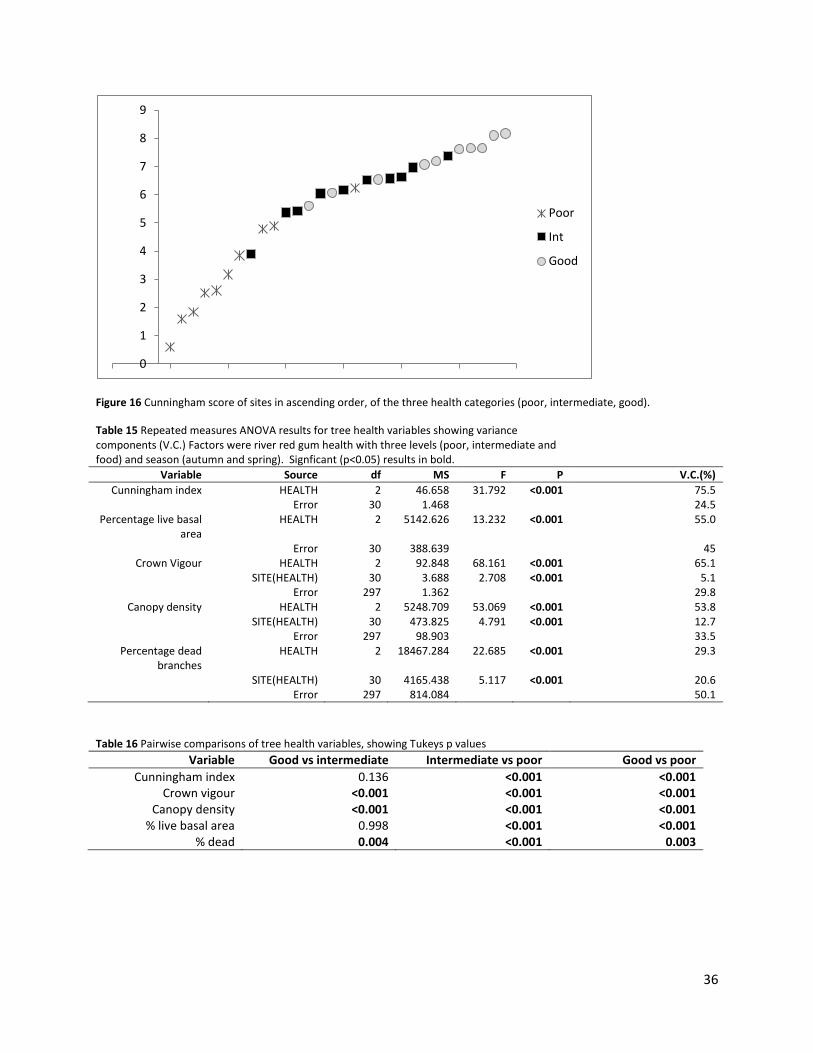
Cunningham score for river red gum health averaged 5.3 (± 0.4 SE, range 0.6-8.2). There was a

continuum of scores, with some overlap: nine out of the ten lowest scored sites were in the

poor category, and seven out of the ten best sites were in the good category (Figure 16).There

was a significant difference in the health score among river red gum health categories (Table

15), with higher scores in good compared to poor sites (Tukeys p < 0.001) and intermediate

compared to poor sites (Tukeys p < 0.001), but not between good and intermediate sites (p =

0.136). Health accounted for 75.5% of the variability in Cunningham scores among sites.

Percentage live basal area averaged 66 (± 4.6SE, range 4.2 - 97.2 %), with a significant

difference among river red gum health categories (Table 15). Again, this was higher in good

compared to poor, good compared to intermediate, but not between good and intermediate

(Table 16, Figure 17). Crown vigour, canopy density also differed among all river red gum

categories showing denser more full canopies at sites of better health (Table 15, Table 16). The

percentage of dead branches was also higher at poor sites (Table 15, Table 16).

Further, there were clear differences in habitat structure among river red gum health

categories with a two-dimensional PCA explaining 46.3 % of the variation among sites (Figure

19). The different river red gum health categories were differentiated along the PC1 axis, with

leaf litter, canopy density, understorey green-ness, canopy height and herb cover

corresponding to negative loadings on PC1, while bare ground, shrub cover and understorey

height had positive loadings (Table 18). Good sites were typified by tall trees with dense

canopy, more leaf litter and low green herbaceous understorey, while poor sites had small

trees with thin canopy, more bare ground and tall, dry, shrubby understorey (Figure 19, Figure

21, Figure 22, Figure 23). Flood history was significantly correlated with tree health variables

(BEST analysis, Rho = 0.337, p = 0.02). There was also a significant negative relationship

between the Cunningham index and time since last flood and flood frequency (Figure 24, Figure

15).

35

Twenty seven plant taxa were recorded with a minimum of five percent cover in at least one

quadrat (Appendix 2). Aquatic species were only found at good sites, and herbs were mainly

found at good sites (Figure 28). Larger water dependent plants (lignum and common reed)

were most abundant at good sites (Figure 28). These differences in overall understorey

structure are summarised in Figure 28. The genus Einadia, a generally low shrub, was the most

common species, found at 93 percent of sites. The next most common taxa were Sclerolaena,

Atriplex and Maireana (Figure 25). Bare ground and leaf litter were also significant components

of the ground cover at most sites. Five good sites had standing water during the autumn survey,

which had mostly subsided by spring. Understorey community composition varied significantly

between all pairs of river red gum health categories (Table 19, Figure 26). Understorey of good

sites was much more variable than intermediate and poor sites (PERMDISP average deviations

from centroid 37.48, 27.27 and 23.83 respectively). There was a significant correlation between

tree health variables and understorey composition (BEST Rho = 0.519, p = 0.001), best

explained by crown vigour and the presence of mistletoe. Four cover types, Einadia, bare

ground, leaf litter and Sclerolaena, contributed > 90% of the similarity among poor sites.

Contrastingly, six and seven cover types drove patterns at intermediate and good river red gum

health respectively (Table 20). Einadia, bare ground and leaf litter were common to all river red

gum health categories. Bare ground was more abundant at poor sites, while leaf litter was more

abundant at good sites. Lippia, clover and water contributed to similarities among good sites

and were not found at any poor sites while Maireana contributed only to intermediate, and

Atriplex to good and intermediate sites (Table 20). Sclerolaena was found at all poor and

intermediate sites but only at 20% of good sites. The same cover types were among a more

extensive list of species contributing to the dissimilarities among river red gum health

categories (Table 20). Atriplex, Maireana, Enchylaena and Chenopodium were most abundant

at intermediate sites (Table 20). Average and maximum understorey height differed

significantly among all river red gum health categories (F2,27 = 25.374, p = 0.001; F2,27 = 3.936, p

= 0.021) (Figure 27).

36

Figure 16 Cunningham score of sites in ascending order, of the three health categories (poor, intermediate, good).

Table 15 Repeated measures ANOVA results for tree health variables showing variance components (V.C.) Factors were river red gum health with three levels (poor, intermediate and food) and season (autumn and spring). Signficant (p<0.05) results in bold.

Variable Source df MS F P V.C.(%)

Cunningham index HEALTH 2 46.658 31.792 <0.001 75.5 Error 30 1.468 24.5

Percentage live basal area

HEALTH 2 5142.626 13.232 <0.001 55.0

Error 30 388.639 45 Crown Vigour HEALTH 2 92.848 68.161 <0.001 65.1

SITE(HEALTH) 30 3.688 2.708 <0.001 5.1 Error 297 1.362 29.8

Canopy density HEALTH 2 5248.709 53.069 <0.001 53.8 SITE(HEALTH) 30 473.825 4.791 <0.001 12.7 Error 297 98.903 33.5

Percentage dead branches

HEALTH 2 18467.284 22.685 <0.001 29.3

SITE(HEALTH) 30 4165.438 5.117 <0.001 20.6 Error 297 814.084 50.1

Table 16 Pairwise comparisons of tree health variables, showing Tukeys p values

Variable Good vs intermediate Intermediate vs poor Good vs poor

Cunningham index 0.136 <0.001 <0.001 Crown vigour <0.001 <0.001 <0.001

Canopy density <0.001 <0.001 <0.001 % live basal area 0.998 <0.001 <0.001

% dead 0.004 <0.001 0.003

0

1

2

3

4

5

6

7

8

9

Poor

Int

Good

Figure 17 Mean values (±SE) for tree health variables across the health categories.

Good Int Poor

HEALTH

0

10

20

30

40

50

60

70

80

90

100

Pe

rce

nta

ge

liv

e b

asa

l a

rea

Good Int Poor

HEALTH

0

10

20

30

40

Ca

nop

y d

en

sity

Good Int Poor

HEALTH

0

10

20

30

40

50

60

Cro

wn

vig

ou

r

Good Int Poor

HEALTH

0

1

2

3

4

5

6

7

8

9

Cu

nn

ing

ha

m s

co

re

Good Int Poor

HEALTH

-0.2

0.0

0.2

0.4

0.6

0.8

1.0

Ho

llow

s

38

Table 17 ANOVA results for abundances of the four size classes of river red gum(R.R.G.) (dead and live trees have been pooled), showing variance components (V.C.) Health has three levels (good, intermediate and poor).

Source R.R.G. 2-10cm (log) R.R.G. 10-50cm (log) MS F p V.C. MS F P V.C.

Health 9.571 5.88 0.004 31.3 2.998 3.888 0.022 22.4 error 1.722 68.7 0.771 77.6

Source R.R.G. 50-100cm (log) R.R.G. >100cm (log) MS F p V.C. MS F P V.C.

Health 0.855 2.056 0.130 9.5 0.533 1.979 0.140 8.9 error 0.416 90.5 0.269 91.1

Figure 18 Mean abundances of trees in each of eight size classes by diameter at breast height (cm), both alive (L) and dead (D).

Figure 19 Average proportion of river red gums with hollows, mistletoe and fruit or buds by health category (good, intermediate and poor) (±SE)

0

5

10

15

20

25

Good Int Poor

Ave

rage

ab

un

dan

ce p

er

40

0sq

.m

HEALTH

D100+

L100+

D50-100

L50-100

D10-50

L10-50

D2-10

L2-10

Good Int Poor

HEALTH

0.0

0.1

0.2

0.3

0.4

0.5

0.6

Mis

tle

toe

Good Int Poor

HEALTH

-0.2

0.0

0.2

0.4

0.6

0.8

1.0

Riv

er

red

gu

m f

ruits

39

Figure 20 PCA of sites based on habitat structure, showing structural changes with health decline along the PC1axis. PC1 and PC2 account for 46.3% of the variation between sites. The variables are bare ground (bare), canopy density (CD), understorey green-ness (Gr), insect damage (ID), herb cover (herb), leaf litter (litter), shrub cover (shrub), tree height (TH) and understorey height (UH)

Table 18 Eigenvector values of habitat structure measured by 12 variables against principal component axes one and two.

Variable PC1 PC2

Bare ground 0.322 -0.005 Leaf litter -0.324 -0.078 Shrub cover 0.440 -0.131 Understorey height 0.214 0.364 Canopy density -0.399 -0.242 Hollows -0.188 0.547 Small coarse woody debris 0.002 -0.227

Large coarse woody debris 0.069 0.056 Understorey green-ness -0.252 -0.396 Insect damage -0.022 -0.443 Canopy height -0.340 0.191 Herb cover -0.416 0.207

40

Figure 21 Examples of sites in the 'good' health category showing low green herb cover, leaf litter, and relatively dense canopy, providing habitat for foliage-specialist woodland birds.

41

Figure 22 Examples of sites in the 'intermediate' health category showing increasing shrub cover, thinning canopies.

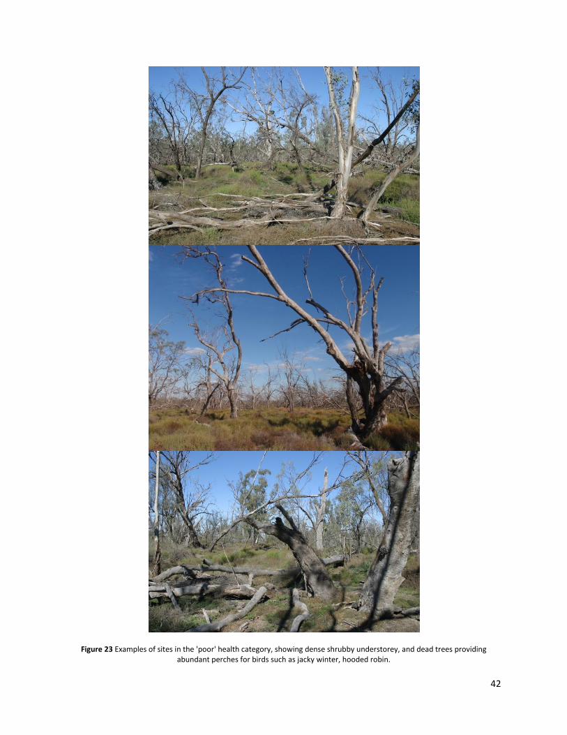
42

Figure 23 Examples of sites in the 'poor' health category, showing dense shrubby understorey, and dead trees providing abundant perches for birds such as jacky winter, hooded robin.

43

Figure 24 Relationships between flood frequency (2001-2006) and Cunningham score (Slope = 0.628, R2 = 0.354), and time

since last flood (at 2006) (Slope = - 0.461, R2 = 0.322), showing regression lines.

Figure 25 Number of sites (maximum 20) at which understorey taxa were found, terrestrial (T) and flood dependent (F) in the three river red gum health categories (poor, intermediate, good).

0 1 2 3 4 5 6 7 8

Flood frequency

0

1

2

3

4

5

6

7

8

9C

un

nin

gh

am

Score

0 1 2 3 4 5 6 7

Time since last flood

0

1

2

3

4

5

6

7

8

9

Cun

nin

gh

am

Score

0

2

4

6

8

10

12

14

16

18

20

Ein

adia

(T)

Scle

rola

ena

(T)

Mai

rean

a (T

)

Atr

iple

x (T

)

Ench

ylae

na

(T)

Lign

um

(F)

Sals

ola

(T)

Spro

uts

Clo

ver

Sto

rksb

eak

(T)

Ree

ds

(F)

Ch

eno

po

diu

m(T

)

No

ogo

ora

Bu

rr (

T)

Dai

sy 2

(T)

Gra

ss (

T)

This

tle2

(T)

Lip

pia

(F)

Ran

un

culu

s (F

)

Flea

ban

e

This

tle

Per

sica

ria

dec

ipie

ns

(F)

Dai

sy1

(T)

Ch

aro

ph

yte

(F)

Dai

sy3

(T)

Nar

do

o (

F)

Nu

mb

er

of

site

s

Species

Good

Int

Poor

44

Table 19 PERMANOVA results based on understorey composition showing variance components (V.C.) Factors were river red gum health with three levels (poor, intermediate and food) and season (autumn and spring). Signficant (p<0.05) results in bold.

Source df MS Pseudo-F P (perm) Unique perms V.C. (%)

BETWEEN SUBJECTS

Health 2 42435 8.6819 0.001 999 35.7

Site(Health) 27 4887.7 7.72 0.001 998 4.0

Residual 270 633.13 60.2

WITHIN SUBJECTS

Season 1 10821 5.0162 0.004 999 1.5

Health x Season 2 4219.4 1.9559 0.066 999 1.2

Site (Health) x Season 27 2157.3 1.1301 0.168 997 0.1

Residual 569 1908.9 97.2

Total 599

Figure 26 MDS of sites based on understorey composition for both spring (s) and autumn (a) surveys. The distribution of study sites of woodland bird communities composition in three categories of river red gum health (poor, intermediate and good) in autumn and spring defined by multidimensional scaling (MDS) in three dimensional ordination space .

45

Table 20 Average abundances (N.) and SIMPER contributions to similarities (%C) for all understorey cover types contributing at least 1% similarity within groups or dissimilarity between river red gum health groups: good (G), intermediate (I) and poor (P)

Cover Good Intermediate Poor G vs I G vs P I vs P N (% C) N (% C) N (% C)

Leaf litter 37.05 (42.78) 33.38 (28.39) 16.72 (18.85) 7.39 11.48 15.65

Bare ground 13.83 (16.92) 18.35 (23.29) 18.58 (25.36) 8.88 8.70 6.42

Einadia sp. 12.83 (14.48) 26.68 (24.59) 41.83 (40.89) 12.06 15.16 11.86

Lippia 9.98 (7.69) 3.35 0.00 10.21 9.47 3.20

Atriplex sp. 3.58 (4.04) 1.57 (5.22) 1.35 6.61 6.14 9.30

Clover 4.80 (2.69) 3.62 0.85 4.41 3.48 3.15

Water 6.80 (2.65) 0.15 0.00 6.32 6.14

Sclerolaena sp. 0.25 2.24 (58.22) 12.72 (11.39) 9.71 11.75 13.17

Maireana sp. 0.65 1.95 (4.06) 0.89 4.33 3.02 6.42

Sprouts 1.90 1.23 0.48 4.38 3.67 5.17

Common reed 1.35 1.13 0.15 3.71 2.65 4.03

Chenopodium sp. 1.10 1.9 0.11 3.38 1.77 3.81

Salsola sp. 0.00 0.78 0.35 3.62

Enchylaena sp. 0.18 0.48 0.1 0.96 3.28

Lignum 0.45 0.00 0.5 1.77 2.55

Ranunculus sp. 4.10 0.53 0.00 5.75 4.89

Fleabane 0.375 0.15 0.00 2.57 2.03

46

Figure 27 Mean understorey height (±SE) among three river red gum health categories

Figure 28 Average cover of the main understorey components across the three health categories.

Good Int Poor

HEALTH

0

20

40

60

80

100

120U

nders

tore

y h

eig

ht

(m)

0%

10%

20%

30%

40%

50%

60%

70%

80%

90%

100%

Good Int Poor

Water dependant plants

Terrestrial shrubs

Herbs

Aquatic plants

Leaf litter

Bare ground

Un

der

sto

rey

hei

ght

(cm

)

47

6 Discussion River red gum decline in the Macquarie Marshes is causing a shift in the woodland bird

community composition, consistent with a ‘terrestrialisation’ of the system. Similar abundances

of large river red gum trees across all health categories suggest these woodlands were all once

in good condition, probably supporting similar woodland bird communities to those in good

sites. The changes in woodland bird community were probably linked to changes in the flooding

regime via effects on vegetation (BEST analysis, Figure 15, Figure 24), providing more evidence

for the effects of river regulation and highlighting the importance of floodplain health and

complexity. The dominance of terrestrial shrubs such as Sclerolaena sp. (Table 17) in the river

red gum forests provide further evidence that the ecosystem is becoming more terrestrial.

Simultaneously, the range of flood dependent understorey shrank, occupying only 10% of sites,

although this probably reflected the dry period.

The decline and death of river red gums significantly changed habitat structure for woodland

birds (Figure 19). If loss of structural complexity occurred, a critical factor for avian biodiversity

(Ford 1985b; Gilmore 1985; Recher 1985; Johnson et al. 2007), then species richness, diversity

and abundance should have decreased. It did not except through changes in community

composition (Table 8, Table 10, Figure 11). Rather, the habitat structure changed, favouring a

different community of woodland birds. As canopy cover, herb cover and leaf litter (an

important foraging substrate) decreased, dense terrestrial shrub cover and abundant dead

limbs increased (Figure 19) favouring species such as hooded robin, jacky winter, southern

whiteface, willie wagtail and white-winged chough (Table 11). These species use perches to

detect terrestrial predators and survey the ground layer for prey (Antos et al. 2008). Fairy-

wrens benefited from the invasion of terrestrial shrubs, although living trees and grassy areas

are also important habitat features for them (Parsons et al. 2008). This may explain why this

group was more abundant at intermediate sites, with live trees and terrestrial shrubs, rather

than at poor sites (Table 14, Figure 13). It is also likely that lignum, a flood dependent shrub

that is good habitat for fairy wrens, has decreased in abundance in the Macquarie Marshes.

These findings confirm the importance of managing for structural complexity and recognising

the value of all parts of the habitat (Shelly 2005).

Foliage specialist birds declined as river red gums lost their canopy (Figure 14). Similar patterns

are seen in terrestrial woodlands, with decreasing abundances of foliage-gleaning insectivores

correlated with declining tree health (Ford and Bell 1981; Ford 1985a; Gilmore 1985). River

regulation is probably contributing to declines already occurring in this group. Rufous whistler,

crested shrike-tit, grey fantail, weebill and striated pardalote are already declining in general

across the western-division of NSW (Smith et al. 1994). Live branch specialists such as white-

bellied cuckoo-shrikes and grey butcherbirds are also sensitive to river red gum decline but

there was another group of generalist woodland birds not sensitive to changing river red gum

48

health. This group included red-rumped parrot, peaceful dove, willie wagtail and magpie lark ,

which use a variety of different habitats and have already benefited from open habitat created

by agriculture and land clearing (Smith et al. 1994).

Some woodland bird species have specific habitat or foraging requirements which help to

explain their response to river red gum decline. Crested shrike-tits forage by probing and

gleaning insects from underneath bark (Smith 1985). When river red gums die they shed their

bark, explaining why crested shrike-tits were found almost exclusively at good sites, and only in

live trees. Mistletoe-birds were also only observed in live trees, and are constrained by the

distribution of mistletoe-bearing trees, found almost exclusively at sites in the good health

category. In general parrots were more abundant at good and intermediate sites, possibly

reflecting the higher abundance of river red gum fruits and other seeds. The lower fertility of

declining trees is also likely to be affecting nectarivores, with fewer flowering trees to supply

their high energy needs. Only five honeyeater species were detected in this study, out of a

recorded ten species for the area (Appendix 2); three of these were isolated sightings, and the

others were only observed feeding on insects, not nectar.

River red gum decline may threaten species already listed as threatened or vulnerable. The

vulnerable brown treecreeper was relatively unaffected by river red gum health, although

highest abundances occurred at good sites. Its distribution may be driven by other habitat

variables, such as the availability of large trees (Antos et al. 2008), which may be a long-term

problem where recruitment is low and dead trees fall over. River red gum sites in poor

condition were favoured by the vulnerable hooded robin, contrasting other work indicating an

association with large patches of healthy trees (Oliver and Parker 2006). The superb parrot,

observed incidentally and at one intermediate site, needs mature red gums next to box

woodlands (Ford et al. 2001) and large hollow-bearing trees for nesting (Webster 1998 in Di

Stefano 2002).

Further data could help better define these changes. In this study river red gum health was

treated as a categorical variable with inevitable overlap across the continuum, even though

there were significant differences in canopy health. More measures of this continuum would

help. Longer temporal analysis of woodland bird communities would also determine whether

patterns changed over seasons and years, improving the power to detect smaller differences in

species richness and abundance and enabling analysis of bird breeding, with tree fruiting and

flowering. There could be long term effects of decline in river red gums on woodland birds.

Many woodland birds are long-lived, so the full effects may not be realised, as decreased

breeding success may not be immediately apparent (Ford 1985b). A few nests were observed

incidentally during spring, all near good sites, indicating that poor sites may not provide suitable

49

nesting habitat. Although there was no difference in hollow bearing trees, important nesting

sites for many birds, this will change as dead trees burn, eventually fall over or break down.

Other impacts could also affect the woodland bird community; changes to groundwater access,

exotic species, grazing and prey abundance. River red gums access water from groundwater

resources and so identifying the role of groundwater in river red gum health is particularly

important (Bren 1988; MDBC 2003; Cunningham et al. 2007a). The high variability in tree health

at infrequently flooded sites may reflect different access to groundwater. Groundwater levels

of some of the areas of poor health have dropped over eight metres in the past decade (Jones,

R. NPW, pers. comm). Groundwater and surface-water are probably interconnected. The

potentially interactive effect of grazing may also be important; this study was only on non-

grazed areas. Grazing significantly alters understorey composition, possibly reducing the

structural complexity of vegetation (Jansen and Robertson 2001b), affecting many grazing-

sensitive bird species (Jansen and Robertson 2001a; Martin and McIntye 2007). Grazing could

amplify the effects of river red gum decline on woodland birds. Invasive species are also

changing woodland bird habitat. For example, lippia, an exotic spreading groundcover which

needs moist conditions, was found at 90% of all sites, yet it is unknown to what extent it

excludes native herbs and grasses or how its presence affects woodland birds. Finally, our

understanding of the mechanisms behind the shift in the bird community would be greatly

improved by information on invertebrate prey abundance at sites in different conditions.

Unfortunately, most river red gum forest and woodland areas in the Macquarie Marshes are

already degraded (Figure 16). Due to a lack of baseline data it was not possible to know the full

extent of changes, but woodland bird communities have probably changed throughout the

Macquarie Marshes. Out of 123 woodland bird species previously recorded in the Macquarie

Marshes (excluding nocturnal birds, see Appendix 1), this study detected 85, and one species,

the red-backed kingfisher, not previously recorded. Some of the species not recorded, such as

finches and chats, are more commonly found in more open areas, but it is possible that some

have declined. No sites were in truly good condition, as under the Cunningham system,

seventeen sites would actually be classified poor (6.1-9), eight degraded (3.1-6), and five

severely degraded (0.2-3). The low variability of understorey composition at poor sites

indicated that the Macquarie Marshes have lost the variability of vegetation that once

supported a diverse range of organisms. This study contributes to a growing body of knowledge

around the ecological decline of the Macquarie Marshes, a decline recently prompting the

Australian Government’s Environment Minister Peter Garrett to make a public statement about

‘a likely adverse change in the ecological character of the Macquarie Marshes Ramsar

Site’(Garrett and Tebbutt 2009).

50

Further evidence of a degraded system was the dominance of white-plumed honeyeater across

all sites (Ford et al. 2001). They can exclude small insectivorous birds especially if trees are

stressed and not flowering, aggressively defending lerp patches (Woinarski 1985). Most good

sites of river red gums were in small patches (8 – 65 ha) of relatively healthy trees. Only four

good sites were in a large healthy patch of forest (1,105 ha). Even relatively healthy areas were

probably suffering from increased edge effects, and associated habitat fragmentation. This

represents a further threat to some woodland bird species, due to increased risk of predation,

nest parasitism and decreased prey abundances with fragmentation (Loyn 1985; Zanette et al.

2000;Ford et al. 2001; Oliver and Parker 2006). For example, nesting success of eastern-yellow

robins is lower in small sites ( 55 ha), compared to large sites ( > 3400 ha) (Marchant 1985). My

results may underestimate changes to the woodland bird community, as more sites in truly

good condition would be needed for a full assessment.

There is widespread understanding of the need for environmental flows for aquatic ecosystems

and their dependent biota, including the Macquarie Marshes. We have shown that there

appears to be significant changes to the woodland birds as a result of decreased flows and

declining health of river red gums. The top priority should be to maintain core areas of river red

gums in good condition. They may need to be flooded every one to three years with inundation

lasting four to seven months (Roberts and Marston 2000). The next priority should be to flood

river red gums that are stressed but still alive to improve canopy health and maintain habitat

for foliage dependent bird species.

Significant progress has been made in recent years towards more sustainable river

management, but major impediments still exist. The introduction of environmental flows was a

major achievement, stepping away from the paradigm that water is wasted if it reaches lakes,

swamps or wetlands (Johnson 2005). The introduction of government buyback of water

licences is also positive. For example, 70 000ML have been bought from willing sellers for the

Macquarie Marshes (DECC 2009). Current levels of environmental flow allocations are only

sufficient to sustain parts of systems, forcing managers to make triage decisions, choosing

which elements to save at the cost of others (DECC 2009). These are complex social-ecological

systems (Johnson 2005), that can be hindered by conflicts of interest and institutional lethargy.

The findings of this study have broader conservation implications outside of the Macquarie

Marshes. Firstly, this study emphasises the importance of river red gum forests and riparian

forests in general for maintaining woodland bird diversity. Similar changes in the woodland

bird community are probably occurring in other areas where river red gum health is declining.

On the South Australian River Murray floodplain, about 80% of the trees are stressed, with 20-

30% being severely stressed (MDBC 2003). On the Victorian River Murray floodplain, only about

30% of river red gum stands are in good condition (Cunningham et al. 2006). Only on the

51

unregulated Lower Ovens River are most river red gum stands in good condition. As the extent

of river red gum health decline becomes evident, there is increasing public concern about the

health of these iconic trees (Ker 2009; Morton 2008; Plane 2003). Woodland birds are already

declining across agricultural south-east Australia, largely because of habitat loss, degradation

and fragmentation (Ford et al. 2001). Remnant riparian forests form critical habitat (Jansen and

Robertson 2001b), and so widespread river red gum decline poses a serious threat, especially

for foliage dependent species. Positively, recent moves have been made to protect remaining

areas of river red gum in national parks (Clennell 2009), but this does not address the issue of

water stress. Only when water diversion is reduced to sustainable levels will the maintenance

of river red gum woodlands, and their dependent woodland bird communities, and other

ecological values of river and floodplain systems become possible.

52

7 References ABS. (2008) Water and the Murray-Darling Basin- A Statistical Profile, 2000-01 to 2005-06. Australian Bureau of Statistics, Canberra.

Allan J. D. & Flecker A. S. (1993) Biodiversity Conservation in Running Waters. Bioscience 43, 32-43.

Anderson M. J. (2001a) A new method for non-parametric multivariate analysis of variance. Austral Ecology 26, 32-46.

Anderson M. J. (2001b) Permutation tests for uivariate or multivariate analysis of variance and regression. Canadian Journal of Fisheries and Aquatic Sciences 58, 626-39.

Anderson M. J. & Gorley R. N. (2007) PERMANOVA+ for primer: guide to statistical methods. PRIMER-E, Plymouth.

Antos M. J., Bennett A. F. & White J. G. (2008) Where exactly do ground-foraging birds forage? Foraging sites and microhabitat selection in temperate woodlands of southern Australia. Emu 108, 201-11.

Bacon P. E. (1994) The importance of water availability to river red gum (Eucalyptus camaldulensis) in the Macquarie Marshes. In: Proceedings of the Macquarie Marshes Workshop 1994 pp. 13-9. Macquarie Marshes Total Catchment Management Subcommittee, Dubbo.

Ballinger A. & Lake P. S. (2006) Energy and nutrient fluxes from rivers and streams into terrestrial food webs. Marine and Freshwater Research 57, 15-28.

Barrett G., Silcocks A., Barry S., Cunningham R. B. & Poulter R. (2003) The new atlas of Australian birds. Royal Australasian Ornithologists Union, Hawthorn East, Vic.

Bastow J. L., Sabo J. L., Finlay J. C. & Power M. E. (2002) A basal aquatic-terrestrial trophic link in rivers: algal subsidies via shore-dwelling grasshoppers. Oecologia 131, 261-8.

Beyer H. (2004) Hawth's Analysis Tools for ArcGIS. Available at http://www.spatialecology.com/htools.

Bibby C., Burgess N., Hill D. & Mustoe S. (2000) Bird Census Techniques. Academic Press, London.

Boulton A. J. & Lloyd L. N. (1992) Flooding frequency and invertebrate emergence from dry floodplain sediments of the River Murray, Australia. Regulated Rivers-Research & Management 7, 137-51.

Brander D. (1987) Environmental changes in the southern Macquarie Marshes: 1934-1987. BSc (Applied Geography) thesis, University of NSW, Sydney.

Bren L. J. (1988) Effects of river regulation on flooding of a riparian red gum forest on the River Murray, Australia. Regulated Rivers-Research & Management 2, 65-77.

Bren L. J. & Gibbs N. L. (1986) Relationships between Flood Frequency, Vegetation and Topography in a River Red Gum Forest. Australian Forest Research 16, 357-70.

Briggs S. V., Thornton S. A. & Lawler W. G. (1997) Relationships between hydrological control of River Red Gum wetlands and waterbird breeding. Emu 97, 31-42.

53

Brock M. A., Capon S. J. & Porter J. L. (2006) Disturbance of plant communities dependent on desert rivers. In: Ecology of Desert Rivers (ed R. T. Kingsford). Cambridge University Press, Cambridge.

Bunn S. E., Balcombe S. R., Davies P. M., Fellows C. S. & McKenzie-Smith F. J. (2006) Aquatic productivity and food webs of desert river ecosystems. In: Ecology of Desert Rivers (ed R. T. Kingsford). Cambridge University Press, Cambridge.

Chan E., Yu Y., Zhang Y. & Dudgeon D. (2008) Distribution patterns of birds and insect prey in a tropical riparian forest. Biotropica 40, 623-9.

Chao B. F. (1995) Anthropogenic impact on global geodynamics due to reservoir water impoundment. Geophysical research letters 22, 3529-32.

Clarke K. R. & Gorley R. N. (2006) PRIMER v6: User Manual/ Tutorial. Plymouth Marine Laboratory, PRIMER-E Ltd, Plymouth.

Clarke K. R. & Warwick R. M. (1994) Change in Marine Communities: an Approach to Statistical Analysis and Interpretation'. Natural Environment Research Council, U. K.

Clennell A. (2009) National park plan to save red gums, gain green votes. In: The Sydney Morning Herald. John Fairfax Holdings, Sydney.

Croonquist M. J. & Brooks R. P. (1991) Use of Avian and Mammalian Guilds as Indicators of Cumulative Impacts in Riparian-Wetland Areas. Environmental Management 15, 701-14.

Cunningham R. B., Mac Nally R., White J. G., Read J., Baker P., Thomson J. & Griffioen P. (2006) Mapping the current condition of river red gum (Eucalyptus camaldulensis Dehnh.) stands along the Victorian Murray River floodplain: A report to the northern Victorian Catchment Management Authorities and the Department of Sustainability and Environment. Australian Centre for Biodiversity, Melbourne.

Cunningham S., Read J., Baker P. & Mac Nally R. (2007) Quantitative assessment of stand condition and its relationship to physiological stress in stands of Eucalyptus camaldulensis (Myrtaceae). Australian Journal of Botany 55, 692-9.

Danby R. & Hik D. (2007) Evidence of Recent Treeline Dynamics in Southwest Yukon from Aerial Photographs. Arctic 60, 411-20.

DECC. (2009) Draft Macquarie Marshes Adaptive Environmental Management Plan. Department of Environment and Climate Change, Sydney.

Di Stefano J. (2002) River red gum (Eucalyptus camaldulensis): a review of ecosystem processes, seedling regeneration and silvicultural practice. Australian Forestry 65, 14-22.

EPA. (1995) New South Wales State of the Environment 1995. New South Wales Environmental Protection Authority, Sydney.

ESRI. (2006) ArcGIS version 9.2.

54

Fischer J., Lindenmayer D. B., Blomberg S. P., Montague-Drake R., Felton A. & Stein J. A. (2007) Functional Richness and Relative Resilience of Bird Communities in Regions with Different Land Use Intensities. Ecosystems 10, 964-74.

Ford H. A. (1985a) The bird community in eucalypt woodlands and eucalypt dieback in the northern tablelands of New South Wales. In: Birds of Eucalypt Forests and Woodlands: Ecology, Conservation, Management (eds A. Keast, H. Recher, H. A. Ford and D. A. Saunders). Surrey Beatty and Sons, Chipping Norton, NSW.

Ford H. A. (1985b) A synthesis of the foraging ecology and behavious of birds in eucalypt forests and woodlands. In: Birds of Eucalypt Forests and Woodlands: Ecology, Conservation, Management (eds A. Keast, H. Recher, H. A. Ford and D. A. Saunders). Surrey Beatty and Sons, Chipping Norton, NSW.

Ford H. A., Barrett G. W., Saunders D. A. & Recher H. F. (2001) Why have birds in the woodlands of Southern Australia declined? Biological Conservation 97, 71-88.

Ford H. A. & Bell H. (1981) Density of birds in eucalypt woodland affected to varying degrees by dieback. Emu 81, 202-8.

Garrett P. & Tebbutt C. (2009) Joint press release: planning for the future of the Macquarie Marshes. http://www.environment.gov.au/minister/garrett/2009/mr20090820.html accessed 10/9/2008.

Gehrke P. C., Brown P., Schiller C. B., Moffatt D. B. & Bruce A. M. (1995) River-regulation and fish communities in the Murray-Darling River system, Australia. Regulated Rivers-Research & Management 11, 363-75.

Gende S. M. & Willson M. F. (2001) Passerine densities in riparian forests of southeast Alaska: Potential effects of anadromous spawning salmon. Condor 103, 624-9.

George A., Walker K. F. & Lewis M. (2005) Population status of eucalypt trees on the River Murray floodplain, South Australia. River Research and Applications 21, 271-82.

Gilmore A. M. (1985) The influence of vegetation structure on the density of insectivorous birds. In: Birds of Eucalypt Forests and Woodlands: Ecology, Conservation, Management (eds A. Keast, H. Recher, H. A. Ford and D. A. Saunders). Surrey Beatty and Sons, Chipping Norton, NSW.

Gray L. J. (1993) Response of insectivorous birds to emerging aquatic insects in riparian habitats of a tallgrass prairie stream. Am. Midl. Nat. 129, 288-300.

Hnatiuk R. J., Thackway R. & Walker J. (2006) Vegetation Field Methods, Yellow Book. CSIRO.

Huxel G. R. & McCann K. (1998) Food web stability: The influence of trophic flows across habitats. Am. Nat. 152, 460-9.

Jansen A. & Robertson A. I. (2001a) Relationships between livestock management and the ecological condition of riparian habitats along an Australian floodplain river. J. Appl. Ecol. 38, 63-75.

Jansen A. & Robertson A. I. (2001b) Riparian bird communities in relation to land management practices in floodplain woodlands of south-eastern Australia. Biological Conservation 100, 173-85.

55

Johnson M., Reich P. & Mac Nally R. (2007) Bird assemblages of a fragmented agricultural landscape and the relative importance of vegetation structure and landscape pattern. Wildlife Research 34, 185-93.

Johnson W. J. (2005) Adaptive management of a complex social-ecological system: the regulated Macquarie River in south-eastern Australia. M. Res. Sci. Thesis. University of New England, Armidale.

Keith D. (2004) Ocean Shores to Desert Dunes: the native vegetation of New South Wales and the ACT. Department of Environment and Conservation, Hurstville NSW.

Ker P. (2009) $30m rescue bid for parched forest. In: The Age. John Fairfax Holdings, Melbourne.

Kingsford R. T. & Auld K. M. (2003) Waterbird breeding and environmental flow management in the Macquarie Marshes, Arid Australia. In: 9th International Symposium on Regulated Streams pp. 187-200, Albury, AUSTRALIA.

Kingsford R. T., Georges A. & Unmack P. J. (2006) Vertebrates of desert rivers: meeting the challenges of temporal and spatial unpredictability. In: Ecology of Desert Rivers (ed R. T. Kingsford). Cambridge University Press, Cambridge.

Kingsford R. T., Jenkins K. M. & Porter J. L. (2004) Imposed hydrological stability on lakes in arid Australia and effects on waterbirds. Ecology 85, 2478-92.

Kingsford R. T. & Johnson W. (1998) Impact of water diversions on colonially-nesting waterbirds in the Macquarie Marshes of arid Australia. Colonial Waterbirds 21, 159-70.

Kingsford R. T. & Thomas R. F. (1995) The Macquarie Marshes in arid Australia and their waterbirds- a 50 year history of decline. Environmental Management 19, 867-78.

Kingsford R. T. & Thomas R. F. (2004) Destruction of wetlands and waterbird populations by dams and irrigation on the Murrumbidgee River in arid Australia. Environmental Management 34, 383-96.

Klement T. & Jack A. S. (2002) Riverine flood plains: present state and future trends. Environmental Conservation 29, 308.

Lada H., Mac Nally R. & Taylor A. (2007) Genetic reconstruction of the population dynamics of a carnivorous marsupial (Antechinus flavipes) in response to floods. Molecular ecology 16, 2934-47.

Legendre P. & Legendre L. (1998) Numerical Ecology. Elsevier Science, Amsterdam.

Lemly A. D., Kingsford R. T. & Thompson J. R. (2000) Irrigated agriculture and wildlife conservation: Conflict on a global scale. Environmental Management 25, 485-512.

Levene H. (1960) A robust approximate confidence-interval for components of variance. Annals of Mathematical Statistics 31, 534-5.

Loyn R. H. (1985) Birds in fragmented forests in Gippsland, Victoria. In: Birds of eucalypt forests and woodlands: ecology, conservation, management (eds A. Keast, H. Recher, H. A. Ford and D. A. Saunders). Surrey Beatty and Sons, Chipping Norton, NSW.

56

Maheshwari B. L., Walker J. & McMahon T. A. (1995) Effects of river regulation on the flow regime of the River Murray, Australia. Regulated Rivers-Research & Management 10, 15-38.

Marchant S. (1985) Breeding of the eastern yellow robin. In: Birds of eucalypt forests and woodlands: ecology, conservation, management (eds A. Keast, H. Recher, H. A. Ford and D. A. Saunders). Surrey Beatty and Sons, Chipping Norton, NSW.

Maron M., Lill A., Watson D. M. & Mac Nally R. (2005) Temporal variation in bird assemblages: How representative is a one-year snapshot? Austral Ecology 30, 383-94.

Martin T. G. & McIntye S. (2007) Impacts of livestock grazing and tree clearing on birds of woodland and riparian habitats. Conserv. Biol. 21, 504-14.

MDBC. (2003) Preliminary investigations into observed river red gum decline along the River Murray below Euston. Technical Report 03/03. Murray Darling Basin Commission, Canberra.

Morton A. (2008) Action sought on river gums. In: The Age. John Fairfax Holdings, Melbourne.

Nairn L. (2008) Redgum Health in the Macquarie Marshes Nature Reserve. In: Wetlands and Rivers, University of New South Wales.

Nakano S. & Murakami M. (2001) Reciprocal subsidies: dynamic interdependence between terrestrial and aquatic food webs. Proceedings of the National Academy of Sciences of the United States of America 98, 166-70.

Nilsson C., Reidy C., Dynesius M. & Revenga C. (2005) Fragmentation and Flow Regulation of the World's Large River Systems. Science 308, 405-8.

Oliver D. L. & Parker D. G. (2006) Woodland birds of the NSW central Murray catchment: measuring outcomes of the Greening Australia fencing and tree planting program. NSW Department of Environment and Conservation, Queanbeyan.

Palmer G. C. & Bennett A. F. (2006) Riparian zones provide for distinct bird assemblages in forest mosaics of south-east Australia. Biological Conservation 130, 447-57.

Parsons H., French K. & Major R. E. (2008) The vegetation requirements of Superb Fairy-wrens (Malurus cyaneus) in non-urban edge and urbanised habitats. Emu 108, 283-91.

Plane T. (2003) The bare fact- iconic gums plainly hurting. In: The Australian. Nationwide News.

Polis G. A., Anderson W. B. & Holt R. D. (1997) Toward an integration of landscape and food web ecology: The dynamics of spatially subsidized food webs. Annual Review of Ecology and Systematics 28, 289-316.

Pyke G. & Recher H. (1984) Censusing of Australian birds: A summary of procedures and a scheme for standardisation of data presentation and storage. Department of Vertebrate Ecology, The Australian Museum.

57

Quinn G. P. & Keough M. J. (2002) Experimental design and data analysis for biologists. Cambridge University Press, Cambridge.

Rayner T. S., Jenkins K. M. & Kingsford R. T. (2009) Small environmental flows, drought and the role of refugia for freshwater fish in the Macquarie Marshes, arid Australia. Ecohydrology In press.

Reid M. A. & Brooks J. J. (2000) Detecting effects of environmental water allocations in wetlands of the Murray-Darling Basin, Australia. Regulated Rivers-Research & Management 16, 479-96.

Richardson D. M., Holmes P. M., Esler K. J., Galatowitsch S. M., Stromberg J. C., Kirkman S. P., Pysek P. & Hobbs R. J. (2007) Riparian vegetation: degradation, alien plant invasions, and restoration prospects. Diversity and Distributions 13, 126-39.

Roberts J. & Marston F. (2000) Water regime of wetland and floodplain plants in the Murray-Darling Basin: a sourcebook of ecological knowledge. CSIRO Land and Water, Canberra.

Roberts T. H. (1987) Construction of Guilds for Habitat Assessment. Environmental Management 11, 473-7.

Sabella A. (2009) Aquatic plant and macroinvertebrate community responses to extended dry periods in the Macquarie Marshes (honours thesis). School of Biological, Earth and Environmental Sciences, Faculty of Science UNSW, Sydney.

Sahagian D. (2000) Global physical effects of anthropogenic hydrological alterations: sea level and water redistribution. Global and Planetary Change 25, 39-48.

Shafroth P. B., Stromberg J. C. & Patten D. T. (2002) Riparian vegetation response to altered disturbance and stress regimes. Ecological Applications 12, 107-23.

Shapiro S. S. & Wilk M. B. (1965) An analysis of variance test for normality (complete samples). Biometrika 52.

Shelly D. (2005) Flora and Fauna of the Macquarie Marshes Region (Draft Report). Department of Infrastructure, Planning and Natural Resources, Dubbo.

Smith P. J. (1985) Woodchip logging and birds near Bega, NSW. In: Birds of eucalypt forests and woodlands: ecology, conservation, management (eds A. Keast, H. Recher, H. A. Ford and D. A. Saunders). Surrey Beatty and Sons, Chipping Norton.

Smith P. J., Pressey R. L. & Smith J. E. (1994) Birds of particular conservation concern in the western division of New South Wales. Biological Conservation 69, 315-38.

Sokal R. & Rohlf R. (1995) Biometry: the principles and practice of statistics in biological research. W. H. Freemand and company, New York.

SRA. (2007) The sustainable rivers audit vegetation theme level 2 assessment pilot study: field protocol (draft). Sustainable Rivers Audit.

58

Stauffer D. F. & Best L. B. (1980) Habitat selection by bird of riparian communities- evaluating effects of habitat alterarions Journal of Wildlife Management. 44, 1-15.

Steinfeld C. & Kingsford R. T. (2008) Floodplain development and vegetation health on the Macquarie River floodplain of the Murray-Darling Basin. School of Biological, Earth and Environmental Sciences. University of New South Wales, Sydney.

Thoms M. C. (2006) Variability, complexity and diversity: the geomorphology of river ecosystems in dryland regions. In: Ecology of Desert Rivers (ed R. T. Kingsford). Cambridge University Press, Cambridge.

Underwood. (1997) Experiments in ecology: their logical design and interpretation using analysis of variance. Cambridge University Press, Cambridge.

UNEP-WCMC. (2001) Biodiversity and climate change. United Nations Environment Programme- World Conservation Monitoring Centre.

Walker K. F. (2006) Serial weirs, cumulative effects, the Lower River Murray, Australia. In: Ecology of Desert Rivers (ed R. T. Kingsford). Cambridge University Press, Cambridge.

Wilson J. B. (1999) Guilds, functional types and ecological groups. Oikos 86, 507-22.

Wilson R. (2008) Vegetation Mapping for the Macquarie Marshes, as part of the Wetland Recovery Program. Unpublished report for the the NSW Department of Environment and Climate Change.

Woinarski J. C. Z. (1985) Foliage-gleaners of the treetops, the pardalotes. In: Birds of eucalypt forests and woodlands: ecology, conservation, management (eds A. Keast, H. Recher, H. A. Ford and D. A. Saunders). Surrey Beatty and Sons, Chipping Norton, NSW.

Woinarski J. C. Z., Brock C., Armstrong M., Hempel C., Cheal D. & Brennan K. (2000) Bird distribution in riparian vegetation in the extensive natural landscape of Australia's tropical savanna: a broad-scale survey and analysis of a distributional data base. J. Biogeogr. 27, 843-68.

Zanette L., Doyle P. & Tremont S. M. (2000) Food shortage in small fragments: Evidence from an area-sensitive passerine. Ecology 81, 1654-66.

59

Appendix 1: Bird species list- Macquarie Marshes, May-August 2009 Order Family Common Name Scientific Name Spatial

guild Number observed

Casuariiformes Casuariidae 1. Emu Dromaius novaehollandiae

na i

Columbiformes Columbidae

2. Common Bronzewing

Phaps chalcoptera

na 1

3. Crested Pigeon Ocyphaps lophotes

Dead tree branch

75

4. Diamond Dove Geopelia cuneata Dead tree branch

13

5. Peacful Dove Geopelia placida Generalist 35

Coraciiformes Alcedinidae 6. Azure Kingfisher Alcedo azurea na 1

Halyconidae 7. Laughing Kookaburra

Dacelo novaguineae

na i

8. Red-backed Kingfisher

Todiramphus pyrrhopygia

na i

9. Sacred Kingfisher Todiramphus sanctus

na i

Cuculiformes Cuculidae 10. Fan-tailed Cuckoo

Cacomantis flabelliformis

na i

11. Horsfield's Bronze Cuckoo

Chalcites basalis na i

12. Pallid Cuckoo Cuculus pallidus na 1

Falconiformes Falconidae 13. Australian Hobby Falco longipennis na i

14. Brown Falcon Falco berigora na i

15. Nankeen Kestrel Falco cenchroides

na 2

16. Spotted harrier Circus assimilis na i

Accipitridae 17. Black-shouldered Kite

Elanus axillaris na i

18. Brown Goshawk Accipiter fasciatus

na i

19. Little Eagle Hieraaetus morphnoides

na i

20. Wedge-tailed Eagle

Aquila audax na i

21. 22. Whistling Kite Haliastur

sphenurus na i

23. White-bellied Sea-Eagle

Haliaeetus leucogaster

na i

Galliformes Phasianidae 24. Brown Quail Coturnix ypsilophora

Ground 6

Passeriformes Alaudidae 25. Rufous Songlark Cincloramphus mathewsi

Dead tree branch

13

60

Order Family Common Name Scientific Name Spatial guild

Number observed

Artamidae 26. Australian Magpie

Gymnorhina tibicien

na 4

27. Grey Butcherbird Cracticus torquatus

Live tree branch

6

28. Masked Woodswallow

Artamus personatus

Live tree branch

55*

29. Pied Butcherbird Cracticus nirgogularis

Live tree branch

11

30. White-breasted Woodswallow

Artamus leucorhynchus

na 2

31. White-browed Woodswallow

Artamus superciliosus

Live tree branch

55*

Campephagidae 32. Black-faced Cuckoo-shrike

Coracina novaehollandiae

Generalist 23

33. White-bellied Cuckoo-shrike

Coracina papuensis

Live tree branch

4

34. White-winged Triller

Lalage tricolor na 2

Climacteridae 35. Brown Treecreeper

Climacteris picumnus

Live trunk/ dead tree branch

118

Corcoracidae 36. Apostlebird Sruthidea cinerea na 0

37. White-winged Chough

Corcorax melanorhamphos

Dead tree branch

10

Corvidae 38. Australian Raven Corvus coronoides

na 6

Dicaeidae 39. Mistletoebird Dicaeum hirundinaceum

na 3

Passeriformes Dicruridae 40. Grey Fantail Rhipidura albiscapa

Foliage 9

41. Magpie Lark Grallina cyanoleuca

Generalist 48

42. Restless Flycatcher

Myiagra inquieta Generalist 11

43. Willie Wagtail Rhipidura leucophrys

Generalist 74

Estrildidae 44. Diamond Firetail Stagonopleura oculata

na i

Hirundinidae 45. Fairy Martin Petrochelidon ariel

na 5

46. Welcome Swallow

Hirundo neoxena na i

Maluridae 47. Superb Fairy-wren

Malurus cyaneus Understorey 149**

48. Variegated Fairy-wren

Malurus lamberti Understorey 3

61

Order Family Common Name Scientific Name Spatial guild

Number observed

49. White-winged Fairy-wren

Malurus leucopterus

Understorey 2

Meliphagidae 50. Blue-faced Honeyeater

Entomyzon cyanotis

na 2

51. Little Friarbird Philemon citreogularis

Foliage 6

52. Spiny-cheeked Honeyeater

Acanthagenys rufogularis

na i

53. Striped Honeyeater

Plectorhyncha lanceolata

na i

54. White-plumed Honeyeater

Lichenostomus penicillatus

Foliage 307

55. Yellow-throated Miner

Manorina flavigula

Foliage 11

Motacilladae 56. Australian Pipit Anthus australis na i

Pacycephalidae 57. Crested Shrike-tit Falcunculus frontatus

Foliage 10

58. Golden Whistler Pacychephala pectoralis

na i

59. Grey Shrike-thrush

Colluricincla harmonica

Generalist 36

60. Rufous Whistler Pacychephala rufiventris

Foliage 12

Pardalotidae 61. Buff-rumped Thornbill

Acanthiza reguloides

na 7

62. Chestnut-rumped Thornbill

Acanthiza uropygialis

na 2

63. Southern Whiteface

Aphelocephala leucopsis

Dead tree branch

3

64. Spotted Pardalote

Pardalotus punctatus

Foliage 2

65. Striated Pardalote

Pardalotus striatus

Foliage 11

66. Weebill Smicrornis brevirostris

Foliage 42

67. Yellow rumped thornbill

Acanthiza chrysorrhoa

Foliage 3

68. Yellow Thornbill Acanthiza nana Dead tree branch

7

Petroicidae 69. Eastern-yellow Robin

Eopsaltria australis

Generalist 26

70. Hooded Robin Melanodryas cucullata

Dead tree branch

13

71. Jacky Winter Micoeca fascinans

Generalist 201

62

Order Family Common Name Scientific Name Spatial guild

Number observed

72. Red-capped Robin

Petroica goodenovii

na 1

Pomatostomidae 73. Grey-Crowned Babbler

Pomatostomus temporalis

na i

Ptilonorhynchidae 74. Spotted Bowerbird

Chlamydera maculata

na i

Sylviidae 75. Australian Reed-Warbler

Acrocephalus australis

na i

76. Little Grassbird Megalurus gramineus

na i

Psittaciformes Cacatuidae 77. Cockatiel Nymphicus hollandicus

na 7

78. Galah Eolophus roseicapillus

Live branch 12

Psittacidae 79. Australian Ringneck

Barnardius zonarius

Generalist 83

80. Blue Bonnet Northiella haematogaster

na i

81. Parrot unid. na

82. Red rumped parrot

Psephotus haematonotus

Generalist 68

83. Red winged parrot

Aprosmictus erythropterus

Generalist 4

84. Superb parrot Polytelis swainsonii

na 2

Turnicidae Turniciformes 85. Quail sp. Ground 15

86. Painted button quail

Turnix varia Ground i

Table 21. Bird species information. ‘i’ indicates incidental observations made outside the dedicated surveys. *masked woodswallows and white-browed woodswallows were observed together in large mixed flocks, totalling 55 birds; **Unidentified fairy-wrens are grouped with superb fairy-wren.

The following woodland bird species have also been recorded at the Macquare Marshes, but were not

recorded on this study (list compiled from Australian Bird Atlas and NPWS atlas of NSW wildlife):

1. Stubble Quail Coturnix pectoralis

2. Bar-shouldered Dove Geopelia humeralis

3. Black Kite Milvus migrans

4. Collared Sparrowhawk Accipiter cirrocephalus

5. Swamp Harrier Circus approximans

6. Black Falcon Falco subniger

7. Peregrine Falcon Falco peregrinus

8. Brolga Grus rubicunda

9. Eastern Rosella Platycercus eximius

10. Pale-headed Rosella Platycercus adscitus

11. Budgerigar Melopsittacus undulatus

12. Blue-winged Parrot Neophema chrysostoma

13. Shining Bronze-Cuckoo Chalcites lucidus

14. Rainbow Bee-eater Merops ornatus

15. Splendid Fairy-wren Malurus splendens

16. Inland Thornbill Acanthiza apicalis

17. Black honeyeater Certhionyx niger

18. Black-chinned honeyeater (eastern subspecies) Melithreptus gularis gularis

19. Singing Honeyeater Lichenostomus virescens

20. Crimson Chat Epthianura tricolor

21. White-fronted Chat Epthianura albifrons

22. Noisy Friarbird Philemon corniculatus

23. White-browed Babbler Pomatostomus superciliosus

24. Chestnut-crowned Babbler Pomatostomus ruficeps

25. Ground Cuckoo-shrike Coracina maxima

26. Crested Bellbird Oreoica gutturalis

27. Olive-backed Oriole Oriolus sagittatus

28. Little Woodswallow Artamus minor

29. Horsfield Bushlark Mirafra javanica

30. Little Grassbird Megalurus gramineus

31. Brown Songlark Cincloramphus cruralis

32. Silvereye Zosterops lateralis

33. Common Blackbird Turdus merula

34. Common Starling Sturnus vulgaris

35. Zebra Finch Taeniopygia guttata

36. Double-barred Finch Taeniopygia bichenovii

37. Plum-headed Finch Neochmia modesta

38. House Sparrow Passer domesticus

64

Appendix 2: Understorey vegetation species list Scientific name Common name

Atriplex Saltbush

Chenopodium Goosefoot, crumbweed, Fat Hen

Conyza sp.* Fleabane

Einadia Saltbush, fishweed

Enchylaena tomentosa R.Br. Ruby saltbush

Erodium cicutarium (L.) L'Her. Ex Aiton* Common storksbill

Maireana Bluebush

Marsilea drummondii A. Braun Nardoo

Muehlenbeckia florulenta Meisn. Lignum

Onopordum acanthium L.* Scotch Thistle

Persicaria decipiens (R.Br.) K.L.Wilson Slender knotweed

Phragmites australis (Cav.) Trin. Ex Steud. Common reed

Phyla nodiflora (L.) Greene* Lippia

Ranunculus sp. Buttercup

Salsola

Sclerolaena Rolypoly, copperburr, poverty bush

Trifolium sp.* Clover

Xanthium occidentale Bertol.* Noogoora Burr

Chara sp. or Nitella sp. Charophytes

Daisy 1**

Daisy2**

Daisy3**

Grass**

Sprouts***

Thistle2**

*indicates introduced species

**indicates species that were not identified but given type names; these species were only

found at one or two sites

***’sprouts ‘ was the name given to small mixed germinating plants, generally in damp

depressions.

65

Appendix 3: Site locations

Name FID Longitude Latitude Health

Struggling Alley 0 147.569385 -30.648705 poor

Poo 2 147.590049 -30.698274 intermediate

Phoenix 4 147.563585 -30.675025 poor

Quail Heaven 6 147.516939 -30.633263 good

Afternoon Tea 9 147.516102 -30.640911 good

Scar Tree 11 147.517708 -30.647026 intermediate

Dinner Plate 12 147.511673 -30.649875 intermediate

Mosquitoe's Playground 18 147.518674 -30.669203 good

Waders Reach 20 147.531451 -30.670616 good

Red gum thicket 23 147.568786 -30.659263 poor

Gentle Giant 25 147.527154 -30.661266 good

Billabong Swans 27 147.532899 -30.658055 poor

Whoopsadaisy 28 147.534764 -30.670341 poor

Coolabah heaven 29 147.519894 -30.625708 good

No complaining 34 147.52622 -30.631488 intermediate

Rice Bubbles 39 147.574885 -30.655873 poor

Morning Tea 45 147.524032 -30.638971 intermediate

Lost binoculars 49 147.52141 -30.635422 good

Mob of goats 56 147.529617 -30.640828 intermediate

Not with a bang 58 147.524202 -30.64928 intermediate

Prickly legs 62 147.540576 -30.671985 poor

Contradiction 64 147.52351 -30.655543 poor

Dead Tree Gully 66 147.529668 -30.654738 poor

Dead Wood 67 147.592926 -30.659596 poor

Nutbush Thistle Limit 68 147.577066 -30.672239 poor

Atadwindi 69 147.571865 -30.637317 poor

Boomanditchydaisy 72 147.52012771700 -30.66441986550 good

Miss Piggy 76 147.51073473000 -30.69938432000 good

Enchanted Puddles 77 147.50802870700 -30.70462367880 good

SpeedyReedy 85 147.58658584300 -30.70445310950 intermediate

All knotted up 87 147.59264818200 -30.65415641490 poor

BogSprout 88 147.51462581800 -30.65731272220 intermediate

Hiccoughs 89 147.53213675000 -30.64754373780 intermediate