Master’s Thesis

The Effect of Radio Channel Modelling

on the Network Performance in

VANET

By

Md. Ashraful Islam

Nasimul Hyder Maruf Bhuyan

Department of Electrical and Information Technology

Faculty of Engineering, LTH, Lund University

SE-221 00 Lund, Sweden

3

Abstract Research in vehicle-to-vehicle communication and the Vehicular Ad Hoc

Network (VANET) are two major fields of growing interest. The advent

and recent development of these concepts foster evolution of the new

paradigm of the transportation system, widely known as Intelligent

Transport System (ITS). Among the numerous challenges in adopting

VANET for ITS, modeling the radio channel is a vital one, because of the

mobility of transmitters and receivers, low elevation of antennae, channel

fading and statistically non-stationary of channels. A channel model has

been proposed that agree with the above mentioned unique characteristics

exist in VANET i.e. Lund model. In this work, we have focused on data

delivery performance at the network layer of VANET under Lund

propagation model and compared the performance with that of some of the

existing models i.e. Three log distance model, Friis model and Nakagami

model which are commonly used for analyzing conventional wireless

communications. Average delay per packet and average packet loss ratio

are the two parameters used for comparing the performance. Simulation

results indicate that Lund Model yields mixed kind of results with all other

propagation loss models in both highway and rural scenario in terms of

average delay per packet and average packet loss ratio as a result of its

more realistic nature.

4

Acknowledgments

First of all we would like to thank to Almighty ALLAH for all His

Blessings. Our Master’s thesis would not exist without the continued

support and guidance of our supervisor Dr. Kaan Bür from Lund

University, Sweden. We would also like to thank to our co-supervisor Dr.

Maria Kihl and our examiner Dr. Fredrik Tufvesson Professor at the

Department of Electrical and Information Technology, Lund University for

providing us valuable guidance time to time. We would also like to thank

our supervisor Maria Erman from Blekinge Institute of Technology,

Karlskrona, Sweden for her support. We would like to thank Lund

University EIT department. Finally, we would like to thank from the

bottom of our heart to our families for their moral, material and emotional

support throughout our Masters studies in Sweden.

Md. Ashraful Islam and Nasimul Hyder Maruf Bhuyan.

5

Table of Contents

Abstract ......................................................................................................... 3

Acknowledgments ......................................................................................... 4

List of Figures ............................................................................................... 7

List of Tables ................................................................................................ 9

List of Acronyms ........................................................................................ 10

1 Introduction ......................................................................................... 11

1.1 Overview of the VANET’s project ............................................. 12

1.2 Overview of the routing protocol for VANET............................ 12

1.3 Goal of this thesis ........................................................................ 13

1.4 Organization of the report ........................................................... 14

2 Literature Review ................................................................................ 15

2.1 What is VANET? .................................................................................. 15

2.2 VANET Application ............................................................................. 16

2.2.1 Safety application ........................................................................... 17

2.2.2 Traffic Management application .................................................... 18

2.2.3 Comfort and Maintenance application ........................................... 19

2.3 Intelligent Transport Systems (ITS) ...................................................... 19

2.3.1 Cooperative Awareness Message (CAM) ...................................... 20

2.3.2 Decentralized Event Notification Message (DENM) .................... 21

2.4 VANET Projects ................................................................................... 22

2.4.1 Projects in Europe .......................................................................... 22

2.4.2 Projects in USA .............................................................................. 23

2.4.3 Projects in Japan............................................................................. 23

2.5 Routing protocol in VANET’s .............................................................. 24

2.5.1 Optimized Link State Routing (OLSR) ......................................... 27

2.5.2 Ad hoc On-Demand Distance Vector (AODV) ............................. 28

2.5.3 Destination Sequenced Distance Vector (DSDV) ......................... 29

3 System model and Simulation.................................................................. 31

3.1 Problem Description ............................................................................. 31

3.2 Simulation Specification: ...................................................................... 32

3.3 NS-3 ...................................................................................................... 34

3.3.1 The “Lund Model” ......................................................................... 35

6

3.3.2 Propagation loss models in NS3 .................................................... 36

3.4 Implementation of our scenario ............................................................ 38

3.4.1 Flow Monitor ................................................................................. 44

3.4.2 Mobility and Positioning ................................................................ 44

3.4.3 Simulation Time ............................................................................. 46

3.5 A More Generic Scenario ..................................................................... 46

4 Experiment Result ............................................................................... 49

4.1 Performance Criteria ............................................................................. 49

4.2 Simulation Setup ................................................................................... 50

4.3 Results of Broadcast........................................................................ 52

4.3.1 Result with Highway scenario ....................................................... 52

4.3.2 Result with Rural scenario ............................................................. 55

4.4 Results of unicast Highway scenario .............................................. 58

4.4.1 Result with AODV ......................................................................... 58

4.4.2 Results with DSDV ........................................................................ 60

4.4.3 Results with OLSR......................................................................... 62

4.5 Result of unicast Rural scenario ...................................................... 63

4.5.1 Result with AODV ......................................................................... 64

4.5.2 Result with DSDV ......................................................................... 65

4.5.3 Result with OLSR .......................................................................... 67

5 Conclusion and future work ................................................................ 69

Future Work ................................................................................................ 71

References ................................................................................................... 72

7

List of Figures

FIGURE 1: APPLICATION OF THE VANET..................................................... 17

FIGURE 2: DROP OF THE ACCIDENTS THANKS TO THE TECHNOLOGICAL

IMPROVEMENT [4]. ............................................................................... 17

FIGURE 3: SCENARIO FOR INTELLIGENT TRANSPORT SYSTEMS (ITS) [31]. .. 20

FIGURE 4: COOPERATIVE AWARENESS MESSAGE (CAM) [17]. ................... 21

FIGURE 5: DECENTRALIZED EVENT NOTIFICATION MESSAGE (DENM) [17].

............................................................................................................. 22

FIGURE 6: THE TAXONOMY OF THE VEHICULAR AD HOC NETWORKS [10]. .... 25

FIGURE 7: OLSR HIERARCHY DIAGRAM IN NS3. ........................................ 28

FIGURE 8: AODV HIERARCHY DIAGRAM IN NS3. ....................................... 29

FIGURE 9: DSDV HIERARCHY DIAGRAM IN NS3. ........................................ 30

FIGURE 10: ROAD STRIP AND SCATTERER DISTRIBUTION FOR HIGHWAY 500

M. ......................................................................................................... 33

FIGURE 11: ROAD STRIP AND SCATTERER DISTRIBUTION FOR HIGHWAY 2 KM.

............................................................................................................. 33

FIGURE 12: ROAD STRIP AND SCATTERER DISTRIBUTION FOR RURAL 500 M. 34

FIGURE 13: ROAD STRIP AND SCATTERER DISTRIBUTION FOR RURAL 2 KM. . 34

FIGURE 14: POSITION OF THE NODES IN HIGHWAY (500 M)........................... 40

FIGURE 15: POSITION OF THE NODES IN HIGHWAY (2 KM). ........................... 40

FIGURE 16: POSITION OF THE NODES IN RURAL (500 M). .............................. 41

FIGURE 17: POSITION OF THE NODES IN RURAL (2 KM). ............................... 42

FIGURE 18: WIFI DATA FLOW IN NS-3. ........................................................ 43

FIGURE 19: HIGH LEVEL VIEW OF FLOW MONITOR ARCHITECTURE [44]. .... 44

FIGURE 20: TRANSMITTER (YELLOW CAR), RECEIVER (ORANGE CAR) AND

OTHER MDNODES. ................................................................................ 47

FIGURE 21: NEW TRANSMITTER (YELLOW CAR), RECEIVER (ORANGE CAR)

AND OTHER MDNODES. ........................................................................ 47

FIGURE 22: AVERAGE DELAY PER PACKET IN HIGHWAY (CAM). ................. 52

FIGURE 23: AVERAGE PACKET LOSS RATIO IN HIGHWAY (CAM). ................ 53

FIGURE 24: AVERAGE DELAY PER PACKET IN HIGHWAY (DENM). .............. 54

FIGURE 25: AVERAGE PACKET LOSS RATIO IN HIGHWAY (DENM). ............. 54

FIGURE 26: AVERAGE DELAY PER PACKET IN RURAL (CAM). ..................... 56

FIGURE 27: AVERAGE PACKET LOSS RATIO IN RURAL (CAM). .................... 56

FIGURE 28: AVERAGE DELAY PER PACKET IN RURAL (DENM). ................... 57

FIGURE 29: AVERAGE PACKET LOSS RATIO IN RURAL (DENM). .................. 58

FIGURE 30: END-TO-END AVERAGE DELAY PER PACKET IN HIGHWAY

(AODV). ............................................................................................. 59

8

FIGURE 31: END-TO-END AVERAGE PACKET LOSS RATIO IN HIGHWAY

(AODV). ............................................................................................. 60


(DSDV). .............................................................................................. 61


(DSDV). .............................................................................................. 61


(OLSR). ............................................................................................... 62


(OLSR). ............................................................................................... 63

FIGURE 36: END-TO-END AVERAGE DELAY PER PACKET IN RURAL (AODV).

............................................................................................................. 64

FIGURE 37: END-TO-END AVERAGE PACKET LOSS RATIO IN RURAL (AODV).

............................................................................................................. 65

FIGURE 38: END-TO-END AVERAGE DELAY PER PACKET IN RURAL (DSDV).

............................................................................................................. 66

FIGURE 39: END-TO-END AVERAGE PACKET LOSS RATIO IN RURAL (DSDV).

............................................................................................................. 66

FIGURE 40: END-TO-END AVERAGE DELAY PER PACKET IN RURAL (OLSR).

............................................................................................................. 67

FIGURE 41: END-TO-END AVERAGE PACKET LOSS RATIO IN RURAL (OLSR).

............................................................................................................. 68

9

List of Tables TABLE 1: SIMULATION SPECIFICATION [12]. ................................................ 32

TABLE 2: SUMMARY OF NS-3 DEFAULT PARAMETERS [11]. ......................... 38

TABLE 3: BROADCAST SIMULATION SPECIFICATION OF CAM AND DENM

[32, 51]. ............................................................................................... 50

TABLE 4: SIMULATION SCENARIO SPECIFICATIONS. ..................................... 50

10

List of Acronyms

BER Bit Error Rate

CCH Control Channel

DI Diffuse scatterer

DSRC Dedicated Short Range for Communications

GSCM Geometry Based Stochastic Channel Model

HVC Hybrid vehicular communications

ITS Intelligent Transportation Systems

IVC Inter-Vehicle Communications

LOS Line of Sight

MAC Media Access Control

MD Mobile scatterer

MIMO Multiple Input – Multiple Output

OBU Onboard Unit

PER Packet Error Rate

RSU Roadside Unit

V2I Vehicle-to-Infrastructure Communications

V2V Vehicle-to-Vehicle Communications

VANET Vehicular Ad hoc Networks

WAVE Wireless Access in Vehicular Environments

WSSUS Wide Sense Stationary Uncorrelated Scatterer

11

CHAPTER 1

1 Introduction

The vehicle-to-vehicle communications or VANETs is currently an

interesting and very popular research area for a variety of applications

including those which have the potential to significantly improve road

safety, convenience as well as comfort to both drivers and passengers,

traffic efficiency and plays a crucial role in intelligent transportation

system. The field of inter-vehicular communications (IVC), including

vehicle-to-vehicle communications (V2V), vehicle-to-roadside

communications (V2R) and hybrid vehicular communications (HVC) also

known as VANET. IVC systems were developed by using on-board units

(OBUs) which can communicate without any infrastructure. Within the

transmission range or multi hop the packet distributed can be a single hop.

Without the infrastructure of RVC can’t cover a wide area, and this

communication take place between the vehicles and roadside infrastructure.

The extending range of RVC systems is also called the HVC systems using

other vehicles as routers.

The development of Intelligent Transportation Systems (ITS) aims for

improving of the road safety, security and efficiency of the transportation

systems and in the vehicular communication. And remove the dependence

on cellular networks by offering direct communication between cars or to

and from the roadside with minimal latency.

VANET is a field of growing interest and importance. Especially since the

US Federal Communications Commission (FCC) allocated 75 MHz

between 5.850 - 5.925 GHz for Intelligent Transport Systems (ITS) in

1999, the start of the ISO Communication Access for Land Mobiles

(CALM) standardization in 2001 and the work on IEEE 802.11p which has

been finalized in 2010 [1]. The V2V communication which is working for

the IEEE 802.11p/1609 WAVE (Wireless Access in Vehicular

Environment) is specifically designed for ITS communication systems but

still it has some social, technical and economic issues. Therefore, it has

12

been the topic of continuous and vigorous research and discussion among

academia and industry [3].

The SmartVANET architecture with the dedicated short-range

communications (DSRC) plan which divides road into segments and

assigns a service channel to each segment. This SmartVANET architecture

proposed safety, traffic management and commercial application. It also

combines a segment based clustering technique with a hybrid Medium

Access Control (MAC) mechanism [5].

1.1 Overview of the VANET’s project

Though the characteristics of metropolitan area network (MANET) are very

similar to the one of VANET, the channel models and other protocols

developed for MANET cannot be applied directly to the VANET. In

addition, the channel parameters of a VANET is different from that of

cellular mobile networks in many ways. For example, the antenna height

(both of transmitter and receiver) in a VANET is much lower than that of a

cellular network, the radio signal propagation environment is different,

nodes are highly mobile and the impact of road side scatterers. Several

projects on VANET have been carried out around the world, primarily

focusing on vehicle safety channel modelling for the VANET. One of the

earliest studies on IVC was started by JSK (Association of Electronic

Technology for Automobile Traffic and Driving of Japan) in the early

1980s [4]. Later, California PATH and Chauffeur of EU demonstrated

DRIVE to improve the traffic efficiency. Recently, the problems of

vehicular safety and comfortable driving have been investigated in the

CarTALK2000 project [4]. Since 2002, much research have been conducted

in both industry and academia for the development of VANET. The

Car2Car Communication Consortium is a non-profit organization initiated

by the European vehicle manufacturers in 2004 that wants to increase road

security and efficiency using VANET technologies and guaranteeing inter-

vehicle operability in all Europe [4].

1.2 Overview of the routing protocol for VANET

There are many routing protocols used for ad hoc networks [6, 7]. The main

task of the routing protocol is moving the information from a source to a

destination within minimal communication time with the minimum

consumption of network resources. There are some routing protocols have

been revealed for mobile ad hoc networks, and some of the routing

protocols can be applied directly to VANET. In VANET, there are some

13

difficulty to design a reliable routing protocol, because of the fast vehicles

movements and the road scatterers, dynamic information exchange and

relative high speed of mobile node movements. So finding and maintaining

routes for vehicular communication is a very challenging task. In addition,

a realistic mobility model is very important for both design and evaluation

of routing protocols in VANETs.

According to the traffic density and mobility of the nodes there are some

routing protocols are proposed for survey the routing protocols for

VANETs. In [50] introduced some routing protocols for VANETs urban

scenario, such as Anchor based street and traffic aware routing (ASTAR),

Connectivity Aware Routing (CAR), Road based using vehicular traffic

information (RBVT), Beacon less routing algorithm for vehicular

environments (BRAVE), The Cross Layer Weighted Position based

Routing (CLWPR), Mobility aware Ant Colony optimization Routing

(MARDYMO) and Geographic Stateless VANET Routing protocol

(GeoSVR). The dynamic source routing (DSR), ad hoc on demand distance

vector (AODV) and destination sequenced distance vector (DSDV) are

applied in vehicle to infrastructure (V2I) communication, but this protocol

may reduce the network performance in vehicle to vehicle (V2V)

communication [9]. For this reason a new protocol priority based dynamic

adaptive routing (PDAR) used for priority scheduling adaptive routing

mechanism which has lower delay and lower packet loss ratio to improve

the network performance, but the author did not integrate the factor of node

mobility into the transmission condition [9]. In this thesis, we survey the

most recent research progress in mobility channel model and the routing

protocols in VANETs. The next chapter we will describe some routing

protocols of VANETs.

1.3 Goal of this thesis

The goal of this thesis is to investigate the impact of channel modeling on

the network performance in VANET. To do this, different propagation

pathloss models (Three Log Distance. Friis and Nakagami) were compared

with Lund Propagation pathloss model in Highway and Rural scenarios.

The Average Delay per Packet and Average Packet Loss Ratio were the

measurement criteria. Simulation methodology is used in the investigation

by NS-3. In this thesis the following research question is considered:

14

What will be the effect of the Lund propagation pathloss model

comparing with other propagation pathloss models on network

performance in NS-3?

In particular, what effect average packet loss ratio and average delay

per packet have on Lund model along with other propagation pathloss

model in different scenarios (Highway and Rural for different road

lengths?

1.4 Organization of the report

The rest of the report is structured as follows; In Chapter 2 overview of

related background work along with the literature study is presented about

the topics related to the thesis which includes ITS and routing protocols. In

Chapter 3, simulation scenario is explained along the introduction of NS-3

simulator and discussed in detail with the system model of our simulation.

The Chapter 4 deals with all the results of our simulations and their detailed

analysis to find out the answers to our research questions. In Chapter 5 the

conclusions and future work have been drawn on the basis of simulation

results and the future work has been proposed.

CHAPTER 2

2 Literature Review

In the last decade, a lot of work has done in the field of vehicular ad hoc

networks (VANETs), a subclass of mobile ad hoc networks (MANETs) and

it has given birth to a new concept called intelligent transportation system

(ITS). IEEE 802.11p supports the Intelligent Transportation Systems (ITS)

applications such as traffic and accident control, cooperative safety,

emergency warning and intersection collision avoidance. In the Intelligent

Transportation System (ITS) environment, the IEEE 802.11p enhancements

to the previous standards enable robust and reliable vehicle-to-vehicle and

vehicle-to-infrastructure communications by addressing the challenges such

as rapidly changing multipath conditions, doppler shifts and the need to

quickly establish a link and exchange data in very short time (less than 100

ms). Further the enhancements are defined to support other higher layer

protocols that are designed for the vehicle environment, such as the set of

IEEE 1609 standards for Wireless Access in Vehicular Environment

(WAVE). ITS is the combination of all the information of the road

environment and vehicles. The important part of the wireless network

simulation is to check the suitability of a proposed propagation pathloss

model to set as an established channel model [11]. Now a days there are lot

of research going on designing an efficient propagation loss model for

VANET. In [12] VANET mobility and propagation are two main concern

for a propagation pathloss model but there are very limited tools available

in the world to simulate a new propagation pathloss model.

2.1 What is VANET? The vehicle-to-vehicle communications or VANETs are currently a very

popular research area and an interesting implementation platform for a

variety of applications including those which have the potential to

significantly improve road safety. The field of inter-vehicular

communications (IVC), including vehicle-to-vehicle communications

(V2V), vehicle-to-roadside communications (V2R) and hybrid vehicular

communications (HVC) also known as VANET. IVC systems were

16

developed by using on-board units (OBUs) which can communicate

without any infrastructure. Within the transmission range or multi hop the

packets are distributed can be a single hop. Without the infrastructure of

RVC can’t cover a wide area and this communication take place between

the vehicles and roadside infrastructure. The extending range of RVC

systems is also called the HVC systems using other vehicles as routers.

Intelligent Transportation System (ITS) has been developed to improve the

safety, security and efficiency of the transportation system and vehicular

communication remove the dependence on cellular networks by offering

direct communication between cars or to and from the roadside with

minimal latency [4].

Vehicle-to-vehicle communications or VANETs is a field of growing

interest and importance. Especially since the US Federal Communications

Commission (FCC) allocated 75 MHz between 5.850 - 5.925 GHz for

Intelligent Transport Systems (ITS) in 1999, the start of the ISO

Communication Access for Land Mobiles (CALM) standardization in 2001

and the work on IEEE 802.11p which has been finalized in 2010 [1].

The SmartVANET architecture with the DSRC channel plan which divides

road into segments and assigns a service channel to each segment. This

SmartVANET architecture proposed safety, traffic management and

commercial application. It also combines a segment based clustering

technique with a hybrid Medium Access Control (MAC) mechanism [5].

The main goal is provided by VANET systems is the security (reducing

accidents and alleviating accident damages), ecology (reducing traffic

congestion and pollution), comfort (driver assistance, entertainment, etc.)

and efficiency (traffic monitoring) of daily road travel. In the wireless

communications VANET is the unique area of the car industry, which has a

large number of possible applications and resources [4].

2.2 VANET Application

In VANETs we can divide a large number of applications into three

different groups.

17

Figure 1: Application of the VANET.

2.2.1 Safety application

Each year there are less than 300 people dying in Sweden, around 43000

(one in every 12 minutes) in the USA with 6.2 million of police reported

traffic accidents (one in every 5 seconds) and the economic impact of the

traffic related road accident is 230 billion of dollars [4].

The technological improvement of the security measures in a car decreases

the number of accidents and mortality on the street. VANETs systems can

revolutionize the current driving concept with a radical improvement in

safety, as Figure 2 depicts,

Figure 2: Drop of the accidents thanks to the technological improvement [4].

Application

Traffic

management

Application

Comfort-maintenance

Application Safety Application

18

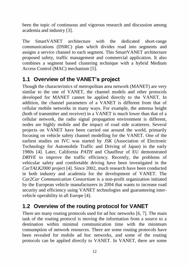
In a busy traffic when an initial collision occurs between the two vehicles

and if the impossibility of breaking on that times for the driver then the

chain of collision occur in the following vehicles. The operator of the

vehicle was provided warning at least one-half second prior to a collision

than 60% roadway collision could be avoided [27]. A system can propagate

safety information for reaction of drivers quicker than a traditional chain of

drivers reacting of their brake light between the cars [4]. The progressing of

the security measures in a car decreases the number of road accidents.

VANET keeps an important role in any uncertain situation on the highway.

If any wheel of a vehicle puncture at night on the highway and the driver

has to stop the vehicle without VANET technology, then he would not send

any warning message to other vehicles to go out of the affected vehicles to

fix it or asking for help (if the driver has no mobile or cannot find any

emergency telephone booth on the highway). And it is a big risk for the

other vehicles on the road. If the vehicle has a VANET system, other

vehicles would detect the emergency message immediately, then the driver

could repair the breakdown in safety conditions or send a message to the

nearest garage to another driver asking for aid [4].

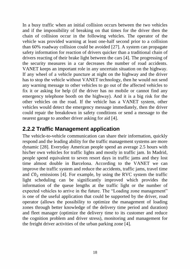
2.2.2 Traffic Management application

The vehicle-to-vehicle communication can share their information, quickly

respond and the leading ability for the traffic management systems are more

dynamic [28]. Everyday American people spend an average 2.5 hours with

his/her own vehicles for traffic lights and mostly in traffic jam. In Madrid,

people spend equivalent to seven resort days in traffic jams and they lost

time almost double in Barcelona. According to the VANET we can

improve the traffic system and reduce the accidents, traffic jams, travel time

and 𝐶02 emissions [4]. For example, by using the RVC system the traffic

light scheduling can be significantly improved which provides the

information of the queue lengths at the traffic light or the number of

expected vehicles to arrive in the future. The “Loading zone management”

is one of the useful application that could be supported by the driver, road

operator (allows the possibility to optimize the management of loading

zones through better knowledge of the delivery time period and duration)

and fleet manager (optimize the delivery time to its customer and reduce

the cognition problem and driver stress), monitoring and management for

the freight driver activities of the urban parking zone [4].

19

2.2.3 Comfort and Maintenance application

The comfort application used for making the travel more pleasant. The

parking spot location, cooperative glare reduction, enhanced route

guidance, GPS correction, instant message, mobile media services and

mobile access to vehicle data [29].

Maintenance application is used to prevent an accident and avoid car

problems. The safety recall notice, wireless diagnostics, time repair

notification and software update [29].

2.3 Intelligent Transport Systems (ITS)

ITS is the one, which is used in an effort to enhance the efficiency, quality

and reliability of different information and telecommunications and for

reliable transport infrastructure. In [30] the ITS services also covers the

area of better and optimized fuel consumption, because the energy

requirements are increasing in today’s world and the resources of energy

are stretched to limits and new research efforts are in process to find the

new and renewable energy sources, so in this environment of less and

expensive energy resources ITS plays a vital role in better and optimum

fuel consumption. The ITS system not only limited to the road transport,

but also it depends on the other transportation domain including aviation,

maritime and railway. In [31] the relay of the ITS is used in radio

communication and wired technologies. In figure 3 we have shown the

complete range of the ITS communication.

ETSI is one of the respected and important standardization organization

which is recognized by the European Union as a European standards

organization. The domain of ITS also falls under the ETSI and it is the

responsibility of ITS to support with comprehensive standardization

activities [30]. The Technical Committee Intelligent Transport System (TC

ITS) is the special committee of ETSI which takes care of all

standardization of ITS [30]. Since the road accident is the main global issue

for the ETSI, it cooperates closely with other international standard

organizations such as International Organization for Standardization (ISO),

European Committee for Standardization (CEN), Electrical and Electronics

Engineers (IEEE) etc. [30, 31].

20

Figure 3: Scenario for Intelligent Transport Systems (ITS) [31].

According to the road traffic environment, there are two main message

models.

1) Cooperative Awareness Message (CAM).

2) Decentralized Event Notification Message (DENM).

2.3.1 Cooperative Awareness Message (CAM)

The Cooperative Awareness Message (CAM) standard is one of the

reference architecture defined by the European Telecommunications

Standards Institute (ETSI) for geographically transmitting data and relevant

information for every vehicle within its range of communication. Within a

single hop distance the CAM message generally consists of message

identifier, station type, speed, acceleration, curvature geographical location

of the vehicles and the basic status of neighboring vehicles to

communicating vehicles. They cannot contain destination address. The

interval of CAMs transmission varies from 0.1 second to 1.0 second

depending on the application, but generally mostly applications uses 0.1

second which are equal to 10 Hz frequency [30]. All the vehicles within the

system must be able to transmit and receive these messages. It is the basic

form of ITS message and it constitutes the overwhelming majority of

21

messages that are transmitted and received in the network [32]. In the figure

depicts the highway CAM scenario where all of the vehicles are

simultaneously transmit and receive the CAM from each other too.

Figure 4: Cooperative Awareness Message (CAM) [17].

2.3.2 Decentralized Event Notification Message (DENM)

Decentralized event notification message (DENM) are generated when

hazardous events (e.g. accidents) has taken place on the road and it is not

routinely transmitted as CAM’s but it is dependent on the happenings of

certain events. DENM does not have any fixed schedule of transmission

and don’t have any destination address. The broadcasting message of

DENM continues till event that triggered the generation of DENM is

present, generally the DENM are generated with high frequency of 20 Hz

and it has a very stringent time delay limits from source to destination [30].

In the following figure the red car has met an accident and transmitting the

DENMs to other vehicles within the vicinity.

22

Figure 5: Decentralized Event Notification Message (DENM) [17].

2.4 VANET Projects

2.4.1 Projects in Europe

In [13] infrastructure deployment, frequency allocation and protocol

definition are three top-priority challenges in Europe. CARTALK (started in

August 2001) was funded IST Cluster support system based on vehicle-to-

vehicle communication (V2V) technologies [4]. During 2001 to 2004

CARTALK2000 was developed as a self-organizing ad hoc radio network

and a cooperative driving assistance system based on the future standards

[4]. In Germany from September 2000 to December 2003 another project

Fleetnet was developed a wireless ad hoc network for inter-vehicle

communications and the solutions of the Fleetnet was based on the UMTS-

UTRA at the data link layer [14]. WILLWARN and INTERSAFE was the

two subproject of VANET [15]. Another project integrated within the EU

was PreVENT which was run until 2007 [4]. Network On Wheels (NOW)

was follow-up project of Fleetnet (2004-2008) [4] and for the safety

applications initial 30 MHz in the frequency band has been used for the

European standard ETSI ITS-G5 [16]. The Car2Car Communication

Consortium is one of the European non-profitable organization initiated by

the European vehicle manufacturers in 2004 that wants to increase road

security and efficiency using VANET technologies and guaranteeing inter-

vehicle operability in all Europe [17]. There are some projects are CVIS-

23

Cooperative Vehicle to Infrastructure Systems [4], COMeSafety[18],

Safespot [19], SeveCom (Secure Vehicular Communications) [20], Coopers

(CO-OPerative SystEms for Intelligent Road Safety) [21], Geonet [22],

iTETRIS [23], Pre-Drive C2X [24] and Have-It project integrates several

advanced vehicle applications for comfort, safety and fuel efficiency [25].

2.4.2 Projects in USA

In USA the initial research and application development started in 2002 and

finished in 2004 for Vehicle Safety Communication (VSC) organization

worked for development the DSRC standard protocols and applications for

vehicle-to-roadside communication and inter-vehicle communication. The

VSC determined 5.9 GHz DSRC wireless technologies had been the

requirement for the VANETs. VSC is some different project like

Cooperative Intersection Collision Avoidance System-Violations (CICAS-

V), Emergency Electrical Brake Light (ERBL), Vehicle Safety

Communications-Applications (VSC-A) [4]. IntelliDrive is one of the

major research project in the USA is the five years (2009-2013) research

consisting in seven tracks to accelerate the development of the V2V

communication system [4]. Different USA University doing significant

research projects such as PATH: California Partners for Advanced Transit

and Highways (administered by university of California, Berkeley), is

currently working on more than 60 projects using the cutting edge

technology in the area of Intelligent Transportation Systems [4].

2.4.3 Projects in Japan

The Advanced Safety Vehicles (ASV) and V2I based Advanced Highway

Systems (AHS) are two main initiatives related vehicle cooperative systems.

The ASV projects are now working in 4th phase. The AHS project is

promoted by Advanced Cruise-Assist Highway Research Association

(ASHRA) [4]. The Smartway project (AVS and AHS) consists of several

communication systems between vehicles and the road, and the variety of

sensors like infrared, cameras, radars, ultrasound, etc. [26]. The important

thing is the transmission of an emergency message via the cross channel

interference problem that cause a car is not receiving the emergency

message. The channel management policies are one of the most efficient

solutions, but it is not the IEEE standard. In IEEE 802.11p have improved

the performance of the receiver requirements in adjacent channel rejections

[4].

24

2.5 Routing protocol in VANET’s

Routing is the process of moving the information across from a source to a

destination. Routing protocol uses for the circuit-switching telephone

network, electronic data networks (Internet) and the transportation network.

In packet switching networks, the routing directs packet forwarding

(packets from their source to the destination) by intermediate nodes. This

intermediate nodes are typically network hardware devices such as routers,

gateways, bridges, firewalls, or switches. General purpose in computers can

also forward the packets and perform the routing, although they are not

specialized hardware and may suffer from limited performance. The routing

process normally directs forwarding on the basis of routing tables which

maintain a record of the destination routes into the networks. Hence,

constructing routing tables, which held in the router's memory, is very

important for the efficient routing. Most routing algorithm uses only one

network path at a time. Multipath routing techniques enable the uses of the

multiple alternative paths.

In case of overlapping equal routes, the following elements are considered

in order to choose which routes get installed into the routing table (sorted

by priority):

1) Prefix-Length: Where longer subnet masks are preferred (independent if

it is within a routing protocol or over different routing protocol).

2) Administrative Distance: where a lower distance is preferred (only valid

between different routing protocols).

3) Metric: where a lower metric/cost is preferred (only valid within one

and the same routing protocol).

Routing, in a more narrow sense of the term, is often contrasted with

bridging in its assumption that network addresses are structured and that

similar addresses imply proximity within the network. Structured addresses

allow a single routing table entry to represent the route to a group of

devices. In larger networks, structured addressing (routing, in the narrow

sense) outperforms unstructured addressing (bridging). Routing has become

the dominant form of addressing on the Internet. Bridging is still widely

used within localized environments [34]. Major applications of VANET

providing safety data, traffic management, toll services, location based

services and documentary [45].

25

VANET routing is classified into unicast, multicast and broadcast

communication. The characterized of VANET routing by dynamic

topology, frequently disconnected network, mobility modeling (varies from

highway of the city environment) and prediction, communication

environment, delay constraints and location identification using sensor [46].

In VANET there are three types of routing protocols namely rural, highway

and urban. The routing protocols on rural area have less network density

and higher mobility. The communication in highway is relatively good

communication in one direction only. In urban environment there are some

challenges for routing protocols; these are node movement which is

bidirectional, traffic density is high in city environment more specifically at

junctions where the density is much higher and also follows any angle as

described in a street map [46].

For the smart ITS system the routing protocols in VANET are an important

and necessary issue because the main difference between VANETs and

MANETs is the rapidly changeable topology and special mobility pattern

[10]. It is not effectively applied the existing routing protocol of MANET

into VANET [10]. Recently, VANET routing protocols are surveyed into

three broad categories; they are unicast, multicast and broadcast routing

protocol [10].

Figure 6: The taxonomy of the vehicular ad hoc networks [10].

26

Most of the recent papers suggest to use DSR, it is a reactive protocol for

routing in MANET and it is also shown that these reactive protocols are not

suitable for higher mobility scenario in VANET because the connectivity of

the network is not known to any node [47]. Also, route repairs and failure

notification overheads lead to low throughput and a high route rediscovery

delay.

Zone based Hierarchical Routing Protocol (ZHLS) is a hierarchical

proactive routing protocol designed for MANET environment that can be

used in VANET in order to improve the performance over other routing

protocols [48]. In this zone based routing protocol roads can be divided into

different geographical segments called zones and the information about

these road segments or zones can be distributed along with the road

information [48]. The benefit of the ZHLS is to take GPS and road

information database in order to improve its routing performance [48].

Anchor based street and traffic aware routing (ASTAR) proposed by

B.C.Seet et al. follows street awareness for efficient routing and also

follows traffic awareness for city environment consists of roads and

junctions that can accommodate more vehicles [46]. As the density

increases, connectivity also increases.

The Connectivity Aware Routing (CAR) protocol proposed by V.Naumov

et al. has four segments namely: Destination location and path discovery,

Data forwarding along the path, path maintenance with the help of guards

and error recovery [49].

Road based using vehicular traffic information (RBVT) protocol proposed

by J.Nzouonta et al. uses real time traffic information to create path either

proactively or on demand and this protocol uses advanced flooding

mechanism which will discard the packet whose address and sequence

number matches that of a previously received packet [46].

Beacon less routing algorithm for vehicular environments (BRAVE) proposed by P.M.Ruiz et al. follows spatial awareness and opportunistic

forwarding. A change from one street to another street is followed when the

distance between the neighbour node of the current junction and the second

junction is less than the actual distance between the two junctions [46].

27

Mobility aware Ant Colony optimization Routing (MARDYMO) protocol

proposed by Correia et al. uses Ant colony optimization in the existing

dynamic MANET On demand (DYMO) protocol which is a reactive

protocol. In order to predict the mobility, position, speed, displacement and

time stamp are added to the Hello message and are sent in a periodic

manner using which the nodes will have updated information on their

neighbors [46].

Geographic Stateless VANET Routing protocol (GeoSVR) proposed by

Y.Xiang et al. routes data using node location and digital map. This

protocol consists of two main algorithms namely, optimal forwarding path

algorithm and restricted forwarding algorithm.

2.5.1 Optimized Link State Routing (OLSR)

In [35] Optimized Link State Routing is a proactive table driven link state

routing protocol which is selecting multipoint relay (MPR) set, also known

as the MPR set of its neighbors such that all its two hop neighbors are

accessible through the MPR set. There are three fold as MPR set are: only

broadcast messages are folded with MPR nodes, link state advertisements

originate only from MPR nodes and MPR nodes can choose the link

between itself and its MPR selector [35]. All of these optimizations serve to

reduce the number of control packets in the network, thus substantially

reducing the overhead compared to other link state protocols. OLSR uses

HELLO and topology control (TC) messages to discover and broadcast link

state information throughout the network [36]. HELLO messages are

periodically sent by a node to its neighbors and contain information about

its MPR selector set (nodes that have chosen it as an MPR node) and it is

not flooded. The topology control messages are used to advertise the MPR

selector set of a node to the entire network and are flooded using the

multipoint relaying system [35]. The advantage of OLSR is the overhead

does not increase with the number of routes required in a network and that a

route is always available when needs [35]. The source code for the OLSR

model it can be found in the directory “src/olsr” in NS-3 and the class

hierarchy is shown in figure below,

28

Figure 7: OLSR Hierarchy Diagram in NS3.

2.5.2 Ad hoc On-Demand Distance Vector (AODV)

Ad hoc On-Demand Distance Vector (AODV) routing protocol is the

combination of both DSR and DSDV protocols because it has basic route

discovery and route maintenance of DSR and uses the hop by hop routing,

beacons and sequence numbers of DSDV [37]. When a route is required,

then the route is discovered because if a route to a destination is not found

in the routing table, the source generates a route request (RREQ) packet and

broadcast it [37]. The RREQ packet contains the source IP address,

broadcast id, current sequence number and most recent sequence number

for the destination known to the source node [37]. The intermediate nodes

update all information about the source node and sets a reverse route entry

to the source [37]. If any intermediate node contains a route to the

destination with a higher sequence number than the one in the RREQ

packet, then it sends a route reply (RREP) to the source otherwise the

packet is rebroadcast until it gets to the destination [37]. On receiving the

packet, the destination sends a unicast RREP back to the source using the

reverse route of the RREQ and each intermediate node sets a forward route

entry to the destination. Each intermediate node also takes note of the

RREQ's source IP address and the broadcast ID so that it does not

rebroadcast a duplicate RREQ [37]. If there is a link breakage on an active

route, the node upstream sends a route error packet (RERR) to the source to

29

inform it that the route is invalid, thus the source can be initiated a route

discovery [38]. The source code for the AODV model it can be found in the

directory ”src/aodv” in NS-3 and the class hierarchy is showing into the

figure below,

Figure 8: AODV Hierarchy Diagram in NS3.

2.5.3 Destination Sequenced Distance Vector (DSDV)

The Destination Sequenced Distance Vector (DSDV) protocol is a

proactive routing table-driven protocol based on the Bellman Ford

algorithm. The tables are periodically updated and the every node in the

network has routing entries for all the nodes in the network [35]. The

highest sequence number of routes is the freshest route and it is the one that

is used [35]. If there are two entries with the same sequence number, the

one with the better metric is used, DSDV uses hop count as its cost metric

[36]. If a node wants to alert the other nodes of an invalid route it sends an

update with an odd sequence number and they know to delete that route

from their table. DSDV uses setting time to dampen route fluctuations [36].

Several protocols have been proposed addressing the challenges of a

routing protocol for VANETs. The source code for the DSDV model it can

be found in the directory “src/dsdv” in NS-3 and the class hierarchy is

shown in figure below,

30

Figure 9: DSDV Hierarchy Diagram in NS3.

31

CHAPTER 3

3 System model and Simulation

In order to fulfill the goal of this thesis, we have to observe the effects of

different radio channel models on the data delivery performance at the

network layer of VANET. For this purpose, the previous work needs to be

integrated into the upper layers of the network protocol stack in NS-3. In

order to put the various alternatives to the test and to evaluate them under

identical, realistic scenarios, computer simulations will be conducted in NS-

3.16. One representative broadcast and unicast protocol were used on top of

the existing (Three log distance Model, Friis Model and Nakagami Model)

and newly integrated propagation loss models (Lund Model) in the scenario

of Lund highway and rural to evaluate the effect of the various radio

channels without routing protocols and with different routing protocols.

This chapter showing a brief overview about the simulation we have used

to model the system.

3.1 Problem Description

Relevant background papers about the routing protocols and propagation

loss models for VANET needed to be studied to understand which kind of

channel models are currently used and how the result from Kåredal et al [1]

differs from the other models using different routing protocols. The first

task was than to adjust the “Lund Model” implementation that was written

for in NS-3.13, by Fabio Heer to the new structure of NS-3.16. The

organization of the network simulator has been significantly changed in the

later release, for example, new directories have been introduced to manage

the growing number of models and names of some of the existing classes

have been changed. The second task was to add flexibility to the “Lund

Model”, so that it can interact well with the upper layers and to make the

model as simple as possible according to the Lund highway and rural

scenario.

The implementation of the “Lund Model” operates with the WiFi-stack and

the mathematical model needs to be verified in NS-3 [1]. When one

32

transmitter sends packets in a periodic interval to a receiver [1]. It supports

an arbitrary number of receivers and in principle also any number of

transmitters [1]. This can be easily realized with a simulation script based

on wifi-phy-test.cc from the WiFi examples. For instance, as in lund-model-

broadcast.cc. In the subsequent chapter, we have discussed more about the

“Lund Model” and the other different propagation loss models

implementations in NS-3.

In this work we have developed the upper layer of the new propagation loss

model (Lund Model) and integrated with the physical layer. We have

constructed the network layer for VANET in accordance with the newly

propagation loss model and compared the performance with the other

existing propagation pathloss models considering the parameters like

average delay per packet and successful average packet loss ratio. The

routing protocol accomplish with the minimal communication time with

minimal consumption of network resources. We have conducted exhaustive

simulations in NS-3 by incorporating various options and evaluated the

performance in both highway and rural scenarios. In addition, we have used

broadcast and unicast protocol on top of the existing propagation loss

models (Friis model, Nakagami models, Three logs distance model) as well

as the newly integrated propagation loss model (Lund propagation model).

Some routing protocols used for MANET with MAC and PHY extension

such as AODV, DSDV and OLSR are already available in NS-3.

3.2 Simulation Specification:

To implement our simulation, we have used the following specifications in

our simulation.

Attribute Name Attribute Value

WAVE operating frequency 5 GHz

WAVE Data Rate 6 Mbps

WAVE Bandwidth 10 MHz

Packet size CAM (200 Bytes)

DENM (100 Bytes)

Frequency of the packet CAM (10 Hz)

DENM (20 Hz)

Highway and Rural street length 500 m; 2 km

Routing Protocols AODV; OLSR; DSDV

Table 1: Simulation Specification [12].

33

The basic scenario used in our simulation is based on the environment of

“Lund Model”. In to the figure below the diffuse scatterer points are shown

in brown (cross), the static discrete are red (circle), the yellow car represent

as a transmitter, red car represent as a receiver, blue car represent as a

mdNodes and the symbols on the road denoted the starting positions of the

cars. In the scenario the line extending from those positions show how far

the vehicles drive during the simulation.

Figure 10: Road strip and scatterer distribution for Highway 500 m.

Figure 11: Road strip and scatterer distribution for Highway 2 km.

34

Figure 12: Road strip and scatterer distribution for Rural 500 m.

Figure 13: Road strip and scatterer distribution for Rural 2 km.

The “Lund Model” is based on the random number for the distribution

(position) of scatters on a road strip, their pathloss exponent n, velocity v,

variance 𝜎𝑠2 of the stochastic amplitude gain and their coherence

distance 𝑑𝑐,𝑟𝑎𝑛𝑑. All of these values are generated in the class

LundModelGeometry.

3.3 NS-3

NS-3 is a discrete-event network simulator, targeted primarily for research

and educational use. NS-3 is free software, licensed under the GNU GPLv2

license, publicly available for development and research use. The goal of

the NS-3 project is to open a simulation environment for networking

research, it should be aligned with the simulation needs of modern

networking research and should encourage community contribution, peer

review, and validation of the software. NS-3 is supported by multiple

35

operating systems, e.g. Microsoft Windows, Linux and Mac OS use

Cygwin. The development of realistic simulation models with the help of

NS-3 infrastructure allows it to be used as a real-time network emulator by

allowing the reuse of many existing protocol implementations within NS-3

[30]. It provides the platform for both IP and non-IP based networks.

However, much research work focuses on wireless/IP simulations involving

WiFi, WiMAX or LTE model for layer 1, layer 2 and static or dynamic

protocols, e.g. OSLR, DSDV and AODV for IP based network [30].

The scripting in NS-3 is mainly done in C++ and Python. Most of the API

is available in Python, but the models are written in C++. We have used

C++ as a programming language in our simulation. It includes rich

environment, allowing users at several levels to customize the information

that can be extracted from the simulations [30].

3.3.1 The “Lund Model”

Relevant background papers on vehicle-to-vehicle communications needed

to be studied to understand, which kind of channel models are currently

used and how the results from Kåredal et al. [2] differs from other models.

At the same time, one had to get familiar with the C++ framework NS-3

through studying the NS-3 tutorial, the manual, the coding style guide and

the API documentation. The final NS-3 implementation of Lund Model

scenario is separated into three classes: LundModel, LundModelGeometry

and LundModelLsFading [1]. The main one, LundModel, inherits the

properties of a propagation loss model and thus integrates easily with the

WiFi stack of NS-3. The class LundModelGeometry deals with the

generation and distribution of static discrete and diffuse scatterers. It keeps

track of the position and the individual parameters of each scatterer [1].

Finally, LundModelLsFading computes the stochastic amplitude gain for

the large-scale fading for each pair of transmitter and receiver; in essence, it

generates sequences of correlated Gaussian values for all paths. To make

use of this class the GNU Scientific Library (GSL) needs to be installed on

the system. Otherwise the model still works, but no large-scale fading is

enabled (the stochastic amplitude gain GS is 0 dB). LundModelTypes

defines commonly used structs in the MD and SD scatters [1].

The user of the "Lund-Model" has complete control over the cars on the

road strip (position and velocity). To simplify the positioning the

implementation provides valid yet random positioning through

GetMobilityHelper. It is the user's responsibility to keep the density of cars

36

reasonable. Static discrete and diffuse scatterers can be created and passed

on via AddSDiscreteScattererers and AddDiffuseScattererers, however, the

"Lund-Model" automatically creates as many of these as required to fit the

specified densities [1]. All that "Lund-Model" needs to know is passed on

by the method Init, which requires a NodeContainer containing all TX

nodes, another one for the RX nodes and a last one for cars that are just

used as mobile discrete scatterers. This method also needs the

communication duration and the interval in which packets are received to

generate time correlated samples for the large-scale fading.

3.3.2 Propagation loss models in NS3

The important task in the wireless network simulation is the choice of the

appropriate propagation loss model for the best performance of any

wireless network channel or set of channels. In [11] variety of such models

varying from abstract, fixed loss models, to a simple exponential decay

proportional to the distance between a transmitter and receiver, accounting

for the ground reflections to models accounting for fast fading. Rappaport

[39] describing the mathematical formulae that can be used for the two

points in a three dimensional space. The some of the NS-3 model equation

are the basis of Rappaport’s equation [11].

Aguayo [40] reports based on the result from a series of measurement

studies based on the existing network in Cambridge (MA, USA) around

MIT called RoofNet. In [11] the RoofNet consists of 38 IEEE 802.11b base

stations mounted on or near rooftops at various points around their campus

and the study uses an active probing technique to measure packet reception

probability at each of the potential receivers for a continuous burst of

packets from a single transmitter [11]. Kotz et. al [41] perform a set of

active measurement experiments, but their approach was to deploy a

temporary network with mobility to measure received signal strength and

reception probability under controlled conditions. In [11] shows that the

measured signal strength as a function of distance can in fact be used to

create a stochastic pathloss model, and that the stochastic model can in fact

produce simulated results that much reasonably well with the measured

field experiments. Recently Zheng and Nicol described a detailed

experiment using an Anechoic Chamber, which is a large room with the

substantial radio signal shielding that essentially isolates the chamber from

outside electromagnetic interference and using this chamber, they measure

and report on the received signal strength for various distances and antenna

characteristics [11].

37

In the NS-3.16 simulation tool has 11 different loss models include

distribution and categorize those loss model into three groups are,

a) Abstract propagation loss models.

1) Fixed Received Signal Strength.

2) Matrix Loss Model.

3) Maximal Range.

4) Random Propagation Loss.

b) Deterministic pathloss models.

1) COST-Hata Model.

2) Friis Propagation Model.

3) Log Distance Pathloss Model.

4) Three log distance Model.

5) Two Ray Ground Model.

c) Stochastic fading models.

1) Jakes Model.

2) Nakagami Model.

Each of the abstract models, as well as each of the pathloss models, are

used in turn, configured with the NS-3 default parameters shown in the

table1.

Propagation Model Default Parameters

Fixed RSS Receive Signal Strength: -150 dBm

Matrix Loss: 1.8 ×10308 dB

Range Maximum range: 250 m

Random Loss: Constant (1 dB)

COST-Hata Center Frequency: 2.3 GHz

Base Station Antenna Height: 50 m

Mobile Station Antenna Height: 3 m

Minimum Distance: 0.5 m

Friis Wave Length: 58.25 mm

System loss: 1

Minimum Distance: 0.5 m

Log Distance Exponent: 3

Reference Distance: 1 m

38

Reference Loss: 46.67 dB

Three log distance Distance: 1 m, 200 m, 500 m

Exponents: 1.9, 3.8, 3.8

Reference Loss at 1 m: 46.67 dB

Two Ray Ground Wave Length: 58.25 mm

System Loss: 1

Minimum distance: 0.5 m

Height above Z: 0 m

Jakes Rays per Path: 1

Oscillators per Ray: 4

Doppler Frequency: 0 Hz

Distribution: Constant (1)

Nakagami Distances: 80 m, 200 m

Exponents: 1.5, 0.75, 0.75

Table 2: Summary of NS-3 default parameters [11].

In our simulation we have used three propagation loss models (Friis,

Nakagami, Three log distance) among the other propagation loss models in

NS-3.16 with Lund highway and rural scenario.

Friis propagation loss model is valid for the free space far field region of

the transmitter antenna. This model is used for the LOS pathloss incurred in

the channel and it is based on the inverse square law of distance which

states that the received power decays by a factor of square of the distance

from the transmitter.

Nakagami channel model is similar to the Rayleigh model, but describes

different fading equations for short-distance and long-distance

transmission. The Rician and the Nakagami model behave approximately

equivalently near their mean value.

Three log distance model is a variation of the log distance model. For

different distance intervals it applies different factors to the logarithmic

pathloss. It is used to predict the propagation loss for a wide range of

environment.

3.4 Implementation of our scenario

We have used both highway and rural scenarios according to the Lund city

environment in our simulation. The Lund model developed by Kåredal et

al. based on the findings three types of scatterers mobile discrete (MD)

39

scatterers represent other cars on the road, static discrete (SD) scatterers

denote buildings, road signs and other prominent obstacles and finally,

diffuse scatterers (DI) model the weak components that result mainly from

the both sides of the 𝑇𝑥 − 𝑅𝑥 path, and this diffuse scatterers are randomly

distributed on a road strip in the 𝑥 − 𝑦 plane [1]. We assumed that a straight

road along the 𝑥-axis of width, 𝑊𝑟𝑜𝑎𝑑 , all the scatterers 𝑥-coordinates are

uniformly distributed over [𝑥𝑚𝑖𝑛, 𝑥𝑚𝑎𝑥]. The 𝑦-coordinates of the MD

scatterers follow a discrete uniform distribution, such that the possible 𝑦-

values fall in the center of the of width, 𝑊𝑙𝑎𝑛𝑒. The SD scatterers 𝑦-

coordinates are Gaussian distributed, symmetrically around the road center.

The DI scatterer points are placed in two uniform intervals with ±𝑌𝐷𝐼 and

width, 𝑊𝐷𝐼 also symmetrically around the road center. The number of

scatterers is dependent on the road length [1]. The scenarios of the other

pathloss models were also based on the scenario of the Lund model’s

density of mdNodes.

Highway:

In our simulation the scenario of the Highway measurement were

performed on 500 m and 2 km long four-lane and each lane was 4.25 m

highway strip cutting through the city of Lund. The total street width was

approximately 17 m. The travel direction separated by a low (≈ 0.5 𝑚)

concrete wall, and the road side environment was characterized by fields or

embankments, the letter constituting a noise barrier for residential areas,

some road signs, few low-rise commercial buildings were located along the

road side and street lamps.

40

Figure 14: Position of the nodes in highway (500 m).

Figure 15: Position of the nodes in highway (2 km).

41

Rural:

Another scenario of our simulation of the Rural measurement were

performed on 500 m and 2 km long two-lane strip cutting just outside Lund,

where the road-side environment contains farm houses, road signs sparsely

along the roadside and some residential house and almost there was no

traffic during these measurements.

Figure 16: Position of the nodes in rural (500 m).

42

Figure 17: Position of the nodes in Rural (2 km).

In our simulation we have designed NS–3 scenario using a simple wireless

adhoc network that allows us to perform a comparative analysis of the

measured network performance (average delay per packet and average

packet loss ratio). In NS-3, nodes contain multiple NetDevice objects; a

simple example can be a computer with different interface cards, e.g. for

Ethernet, WiFi, Bluetooth. When we add a WifiNetDevice to a node that

create models of IEEE 802.11 based infrastructure and adhoc network [30].

As depicted in Figure 18 at the time of transmission WifiNetDevice converts

the IP address to MAC address and add Logical Link Control (LLC) header

to the packet and pass it to AdhocWifiMac which add WiFi Mac header and

estimate the physical mode i.e. the data rate supported by the destination

node.

After that Dynamic Channel Assignment (DCA) DcaTxop class insert the

new packet in the queue and check for another packet transmission or

reception along with a Distributed Coordination Function (DCF) class, if

there is no packet pending, the packet is handed over to the MacLow class

[30]. In case of a pending packet, DcfManager acknowledges the collision

and starts the backoff procedure by selecting a random number and wait to

access again. DcaTxop also checks whether the packet is multicast or it

requires fragmentation or retransmission. When it reaches to the MacLow

43

class of NS-3 it checks if the retransmission was required; it's called the

procedure for retransmission of the packet, if not it sends the packet to the

physical layer of NS-3 named as YansWifiPhy. Which informs the DCF

about the start of transmission, after that the packet is handed over to the

channel class named as YansWifiChannel which estimate the receive power

and set the propagation delay.

Figure 18: Wifi Data Flow in NS-3.

At the receiver side YansWifiChannel hand over the packet to the

YansWifiPhy which calculates the interference level, it drops the packet if

the state of PHY is not idle or the receive power is below the threshold. It

also estimates the packet error rate (PER) from signal to noise ratio. Then

the packet is handed over to the MacLow which check its destination and

send the acknowledgement if the destination is reached. MacRxMiddle

checks whether the received packets is duplicated one with the correct

sequence and passes the packet to the AdhocWifiMac and then to the

44

WifiNetDevice. The AdhocWifiMac was used in the MAC layer and add a

QoS upper MAC.

3.4.1 Flow Monitor

To evaluate the network performance, we have used the Flow Monitor

framework in NS-3 which can be easily used to store and collect network

performance data and counting hop in a network from the NS-3 simulation.

The architectural [44] view of FlowMonitor simulation will typically

contain one FlowMonitorHepler, one FlowMonitor, one Ipv4FlowClassifier

probe capture packets, then ask the classifier to assign identifiers to each

packet, and report on the global the classifier to assign identifiers to each

packet, and report on the global FlowMonitor abstract flow events, which

are finally used for statistically data gathering and for evaluate the network

performance by calculating the packet loss ratio and average delay per

packet.

Figure 19: High Level view of Flow Monitor Architecture [44].

3.4.2 Mobility and Positioning

To make our system model realistic we have assigned the mobility of the Tx

node, Rx node and other mdNodes in the highway and rural scenario at NS-

45

3. The Tx node send the packets towards Rx Node and all other mdNodes

using broadcast and unicast protocol. The mobility module in NS-3

supports the sets of mobility models which are used to track and maintain

the current position and speed of an object. The design includes position

allocators, mobility models and helper functions. The initial position of the

nodes is set with PositionAllocator. Using mobility helper classes most

users interact with the mobility system and the MobilityHelper combines a

mobility model and position allocator, and can be used with a node

container to install mobility capability on a set of nodes [30]. The

ConstantVelocityMobilityModel was used to give a constant velocity to all

mdNodes, Tx and Rx in the scenario. Mobility of the mdNodes, Tx and Rx

are bound to the minimum and maximum of X (0-500 m), X (0-2000 m)

and Y coordinates (4.25 m for Highway and 4m for Rural). Individual car

speeds (mdNodes) were randomly assigned according to a normal

(Gaussian) distribution with the parameters of, Mean Speed = 25 m/s and

Speed Variance = 4.0 m/s.

Generated traffic in our model from Tx to Rx has been implemented with

the help of application module in NS-3. As according to Lund model the

transmitter has the capability to generate packets to the receiver, in this

context we have utilized two application models named OnOff application

and PacketSink application from NS-3 for generation of packets and to sink

them respectively.

Here, is an issue related to the installation of OnOff application that is due

to the simultaneous installation of the application on vehicles that was

limiting number of vehicles according to the vehicles density of the “Lund

Model” [2]. We are using 10 Hz frequency for CAM and 20 Hz frequency

for DENM in the OnOff application to send UDP datagrams of size 200

bytes and 100 bytes respectively [32]. To do this we have installed the

OnOff application on each vehicle at different instance of time. The traffic

generator follow the "On" and "Off" states alternate. The duration of each

of these states is determined with the onTime and the offTime random

variables. During the "Off" state, no traffic is generated. During the "On"

state, packets are generated. This OnOff application is characterized by the

specified "data rate" and "packet size". When an application is started, the

first packet transmission occurs after a delay equal to (packet size/bit rate).

Note also, when an application transitions into an off state in between

packet transmissions, the remaining time until when the next transmission

would have occurred is cached and is used when the application starts up

46

again. In this context, we have utilized two application models named

OnOff application and PacketSink application from NS-3 for generation of

packets and to sink them respectively. In the application layer, OnOff

application was used into the “Lund model”. We have created socket for

UDP implementation by UdpSocketFactory. We have simulated CAM and

DENM without routing and with three different routing protocols (AODV,

DSDV, OLSR) in NS-3.

3.4.3 Simulation Time

The biggest difficulty during our simulations that we faced was the

extraordinary time taken by NS-3 to process the simulations. To give an

idea of how much time the simulations were taking for processing, the basic

scenario of Lund Model will take longer time up to 2 hours of each

simulation and this processing time, sometimes increases when we change

the routing protocols and without routing. The time taken by each simulator

for single run is about 2 hours, which implies after running the code we

have to wait 2 hours for single run result and on the basis of those results

the troubleshooting in the code is done and then run it again and wait for

another 2 hours to get new results. The reason for this extraordinary delay

in simulation processing is the detailed implementation of our simulation

model and according to the NS-3 developers the performance optimization

of the simulator is still in process.

3.5 A More Generic Scenario

In our simulation we have used one Tx, one Rx and some mdNodes

(according to the Lund Propagation pathloss model). We ran our simulation

10 times for two scenarios (Lund highway and rural) to find the answer of

our research question. To use the NS-3 Lund model with different random

number generator we kept the distribution of scatterers and the properties

assigned to them constant in every run and calculated the average of the

result (average packet loss ratio and average delay per packet) [1].

If we want to make our simulation more generic i.e, multiple Tx, Rx are

used randomly for sending and receiving packets by using different

propagation loss models and routing protocols in NS-3. But in Lund

propagation loss model Tx, Rx and mdNodes have different attributes [2]

i.e. velocity, path-loss exponent, variance and coherence distance and those

have given manually in the implementation of our simulation in NS-3. But

if we want to send packets from a new Tx to a new Rx, then old Tx will

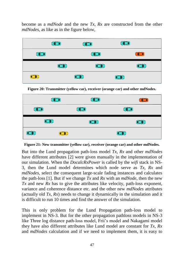
47

become as a mdNode and the new Tx, Rx are constructed from the other

mdNodes, as like as in the figure below,

Figure 20: Transmitter (yellow car), receiver (orange car) and other mdNodes.

Figure 21: New transmitter (yellow car), receiver (orange car) and other mdNodes.

But into the Lund propagation path-loss model Tx, Rx and other mdNodes

have different attributes [2] were given manually in the implementation of

our simulation. When the DocalcRxPower is called by the wifi stack in NS-

3, then the Lund model determines which node serve as Tx, Rx and

mdNodes, select the consequent large-scale fading instances and calculates

the path-loss [1]. But if we change Tx and Rx with an mdNode, then the new

Tx and new Rx has to give the attributes like velocity, path-loss exponent,

variance and coherence distance etc. and the other new mdNodes attributes

(actually old Tx, Rx) needs to change it dynamically in the simulation and it

is difficult to run 10 times and find the answer of the simulation.

This is only problem for the Lund Propagation path-loss model to

implement in NS-3. But for the other propagation pathloss models in NS-3

like Three log distance path-loss model, Frii’s model and Nakagami model

they have also different attributes like Lund model are constant for Tx, Rx

and mdNodes calculation and if we need to implement them, it is easy to

48

implement in NS-3. Moreover, to evaluate the network performance, by

using flow monitor it will be a harder task to fetch the result.

49

CHAPTER 4

4 Experiment Result

This chapter focuses on all the results of simulations findings. There were a

number of simulations run to find the answer of our thesis research

questions. The simulations were set up in such a way that, using CAM and

DENM broadcast and with three different routing protocols specifically the

AODV, DSDV and OLSR were working on different pathloss models. As

the whole simulation scenario has already been defined in detail in the

previous chapter, now the focus will be on its organization and how the

simulations were executed. Before going into the details of simulation

results, it is important to mention that the different pathloss models are

implemented with the same Lund model scenario.

4.1 Performance Criteria

The main performance metrics are defined as follows,

1) Average Delay per Packet: The average time taken by each packet

during its transmission from source to destination. Since ITS had

defined a strict latency requirement for cooperative safety applications,

it makes this parameter as the most important one in judging the

capability of technology for cooperative safety applications in vehicular

communication [30]. Hence the average delay per packet is basically

the total delay of the packet from its transmitter to receiver.

𝐴𝑣𝑒𝑟𝑎𝑔𝑒 𝐷𝑒𝑙𝑎𝑦 𝑝𝑒𝑟 𝑝𝑎𝑐𝑘𝑒𝑡 = 𝑑𝑒𝑙𝑎𝑦 𝑆𝑢𝑚

𝑅𝑥 𝑃𝑎𝑐𝑘𝑒𝑡𝑠 (1)

2) Average Packet Loss Ratio: It is the ratio between the total number of

packets lost to the total number of packets transmitted between

transmitter and receiver.

𝐴𝑣𝑒𝑟𝑎𝑔𝑒 𝑝𝑎𝑐𝑘𝑒𝑡 𝑙𝑜𝑠𝑠 𝑟𝑎𝑡𝑖𝑜 = 𝑙𝑜𝑠𝑡 𝑝𝑎𝑐𝑘𝑒𝑡𝑠

𝑅𝑥 𝑃𝑎𝑐𝑘𝑒𝑡𝑠+𝑙𝑜𝑠𝑡 𝑝𝑎𝑐𝑘𝑒𝑡𝑠 (2)

50

4.2 Simulation Setup

The performance of vehicular communication is evaluated on the basis of

the metrics average delay per packet and average packet loss ratio. The

simulations are divided in two different cases (broadcast and unicast). In

the first case the frequency, packet size, propagation loss models and the

number of mdNodes (500 m 3mdNodes and for 2000 m 10mdNodes) for

highway and (500 m 1mdNodes and for 2000 m 4mdNodes) for rural in

Lund city scenario of broadcast simulation and specified in table 3.

Parameter CAM DENM

Frequency 10 Hz 20 Hz

Packet Size 200 Bytes 100 Bytes

Propagation loss

models

Lund model, Three log

distance model, Friis

model, Nakagami

model

Lund model, Three log

distance model, Friis

model, Nakagami

model

Scenario Highway, Rural Highway, Rural

Table 3: Broadcast simulation specification of CAM and DENM [12, 32].

In second case the frequency, packet size and propagation loss models and

the number of mdNodes (500 m 3mdNodes and for 2000m 10mdNodes) for

highway and (500m 1mdNodes and for 2000m 4mdNodes) for rural Lund

city scenario with routing protocols. The outcome of all the phases of

simulations is presented and discussed in the form of average packet loss

ratio and average delay per packet. The main parameters that define the

difference between the routing protocols are shown in the following Table

4.

Parameter Values

Routing

protocol 1

Routing

protocol 2

Routing

protocol 3

Routing

protocols

AODV DSDV OLSR

Frequency 10Hz 10Hz 10Hz

Packet size 200 bytes 200 bytes 200 bytes

Propagation loss

model

Lund model,

Three log

distance model,

Friis model,

Nakagami model

Lund model,

Three log

distance model,

Friis model,

Nakagami model

Lund model,

Three log

distance model,

Friis model,

Nakagami model

Scenario Highway, Rural Highway, Rural Highway, Rural

Table 4: Simulation scenario specifications.

51

The network performance in VANET was evaluated with Lund propagation

loss model along with some of the existing models, which are commonly

used for analyzing conventional wireless communications. Average delay

per packet and average packet loss ratio are the two parameters used for

comparing the performance. We have used flow monitor for calculating the

average delay per packet and average packet loss ratio. The Flow Monitor

module’s goal is to provide a flexible system to measure the performance of

network protocols. The module uses probes, installed in network nodes, to

track the packets exchanged by the nodes, and it will measure a number of

parameters. Packets are divided according to the flow they belong to, where

each flow is defined according to the probe’s characteristics (e.g., for IP, a

flow is defined as the packets with the same {protocol, source, destination}

tuple). The average delay per packet is basically related with Rx packets

and delay sum. The delay sum contains the sum of all delay for all received

packets of the flows. And the average packet loss ratio is related with lost

packet and Rx packet. For safety vehicular communication we set the

WAVE requirement in our simulation for network performance is 1 ms for

successful packet reception from Tx to Rx and the maximum delay of the

packet at 100 ms [30, 32]. And over 100 ms delay packet, it is treated as a

lost packet [32].

The experiment of the simulation showed a number of results regarding the

overall effect of the chosen pathloss and fading models on the network

performance in VANET. For simulation run, we set up the start time is 10

seconds and the stop time is 20 seconds for the received packet

successfully. Then we run our simulation 10 times to find the answer to our

research questions. This randomness is applied in the state of all the random

variables used in the script, e.g. in our simulation to use the NS-3 Lund

model with different random number generator while keeping the

distribution of scatterers and the properties assigned to them constant in

every run and calculated the average of the result (average packet loss ratio

and average delay per packet) without routing protocols and with the

different routing protocols (AODV, DSDV, OLSR) [1]. We have compared

the newly integrated propagation loss model (Lund model) with other

existing propagation loss model (Three log distance model, Friis model,

Nakagami model) in Lund highway and rural scenario. Furthermore, we

were able to show considerable variation in the computational complexity

of the various models in NS-3.16. Now we are describing the results of

Lund highway and rural scenario in detail below.

52

4.3 Results of Broadcast In VANET we have used the packet size and frequency of CAM and

DENM specification in our simulation. The total number of mobile discrete

(mdNodes) has been tested for the rural and highway scenario.

4.3.1 Result with Highway scenario

In this case in our scenario we have used 200 bytes, 10 Hz frequency for

CAM and 100 bytes, 20 Hz frequency for DENM [12]. The total number of

mobile discrete (mdNodes) has been tested for the highway scenario (3

mdNodes for 500 m and 10 mdNodes for 2 km).

In our scenario the maximum average delay per packet for 2km in Lund

model (around 80 ms) and the minimum average delay per packet in Three

log distance model (around 15 ms). For 2 km the three log distance model,

Friis model and Nakagami model have same (nearly 56 ms) average delay

per packet and for 500 m the Friis model, Lund model and Nakagami

model have same (20 ms) average delay per packet.

Figure 22: Average delay per packet in Highway (CAM).

In this scenario, the CAM has maximum average packet loss ratio 14% for

2 km in Lund model and other models (Three log distance model, Friis

model, Nakagami) have same average packet loss ratio is around 6%. For

500 m Lund model showing the maximum average packet loss ratio is more

0

0.01

0.02

0.03

0.04

0.05

0.06

0.07

0.08

0.09

Three log distance Friis Lund Nakagami

Seco

nd

s

Average Delay Per Packet (CAM)

500m 2000m

53

than 6% and Friis model showing the minimum average packet loss ratio

around 2%.

Figure 23: Average packet loss ratio in Highway (CAM).

For DENM broadcast the maximum average delay per packet is more than

80 ms in Lund model and the other models (Three log distance model, Friis

model, Nakagami model) have almost same average delay per packet is

around 65 ms for 2 km. and for the 500 m the minimum average delay per

packet in Three log distance model is less than 20ms and Friis model and

Nakagami model showing the maximum average delay per packet is more

than 20 ms.

0

0.02

0.04

0.06

0.08

0.1

0.12

0.14

0.16


Ave

rage

Pac

ket

Loss

Rat

io

Average Packet Loss Ratio (CAM)

500m 2000m

54

Figure 24: Average delay per packet in Highway (DENM).

The maximum average packet loss ratio of DENM broadcast is 9% in Lund

model and the other models (Three log distance model, Friis model,

Nakagami model) have same average packet loss ratio is around 7%. For

500 m Lund model showing the maximum average packet loss ratio is less

than 8% in Lund model and Friis model showing the minimum average

packet loss ratio is less than 5%.

Figure 25: Average packet loss ratio in Highway (DENM).

0

0.01

0.02

0.03

0.04

0.05

0.06

0.07

0.08

0.09


Seco

nd

sAverage Delay Per Packet (DENM)

500m 2000m

0

0.01

0.02

0.03

0.04

0.05

0.06

0.07

0.08

0.09

0.1


Ave

rage

Pac

ket

Loss

Rat

io

Average Packet Loss Ratio (DENM)

500m 2000m

55

If we compare the highway result of CAM to the result of DENM, we make

some observations;

1) For 2 km distance Lund model showing the maximum average delay

per packet and other models are almost same average delay per packet

for both case CAM and DENM.

2) For 500 m distance Three log distance model showing the minimum

average delay per packet in both cases.

3) The maximum average packet loss ratio in Lund model and others are

same average packet loss ratio for 2 km.

4) For 500 m distance Lund model showing the maximum average packet

loss ratio and Friis model showing the minimum average packet loss

ratio.

4.3.2 Result with Rural scenario

In our scenario we have used 200 bytes, 10 Hz frequency for CAM and 100

bytes, 20 Hz frequency for DENM. The total number of mobile discrete

(mdNodes) has been tested for the rural scenario (1 mdNodes for 500 m

and 4 mdNodes for 2 km).

In this case, the broadcast rural scenario showing maximum average delay

per packet for 2km in Lund model (around 65 ms) and the other models

have same average delay per packet which is less than 30 ms. For 500 m all

models have same average delay per packet for broadcast which is nearly

10 ms.

56

Figure 26: Average delay per packet in Rural (CAM).

The maximum average packet loss ratio of CAM in Lund model is around

13% for 2 km and other models (Three log distance model, Friis model,

Nakagami model) have same average packet loss ratio is less than 4%. For

500 m the average packet loss ratio is almost same for all propagation loss

models which is around 1%.

Figure 27: Average packet loss ratio in Rural (CAM).

0

0.01

0.02

0.03

0.04

0.05

0.06

0.07


Seco

nd

sAverage Delay Per Packet (CAM)

500m 2000m

0

0.02

0.04

0.06

0.08

0.1

0.12

0.14


Ave

rage

Pac

ket

Loss

Rat

io

Average Packet Loss Ratio (CAM)

500m 2000m

57

The DENM average delay per packet in Lund model is maximum (more

than 60 ms) for 2 km distance. There log distance model and Friis model

showing the same (around 32 ms) average packet loss ratio and Nakagami

model showing the minimum (20 ms) average packet loss ratio. For 500 m

all propagation models showing almost same (10 ms) average delay per

packet in rural scenario.

Figure 28: Average delay per packet in Rural (DENM).

In DENM, average packet loss ratio in Lund model showing the maximum

(around 12%) average packet loss ratio and Nakagami model showing the

minimum (2%) average packet loss ratio in 2 km rural scenario. Three log

distance model and Friis model showing the same (nearly 6%) average

packet loss ratio. For 500 m Nakagami model showing the minimum (less

than 2%) average packet loss ratio and the other models (Three log distance

model, Friis model, Lund model) showing same (2%) average packet loss

ratio.

0

0.01

0.02

0.03

0.04

0.05

0.06

0.07


Seco

nd

s

Average Delay Per Packet (DENM)

500m 2000m

58

Figure 29: Average packet loss ratio in Rural (DENM).

If we compare the rural result of CAM to the result of DENM, we make

some observations,

1) For 2 km distance in rural scenario, the maximum average delay per

packet in Lund model and Nakagami model showing the minimum

average delay per packet.

2) All propagation loss models showing almost the same average packet

loss ratio in 500 m for both case CAM and DENM.

3) The average packet loss ratio in Lund model is maximum for 2 km.

4) For 500 m, the minimum average packet loss ratio is in Nakagami

model.

4.4 Results of unicast Highway scenario

In VANET the packet size has been set to 200 bytes and the frequency is 10

Hz set in the simulation of vehiculer safety application. The total number of

mobile discrete (mdNodes) has been tested for the highway scenario (3


4.4.1 Result with AODV In this case, for AODV routing protocol in our scenario the maximum end-

to-end average delay per packet for 500 m and 2 km in Lund model. For

500m the end-to-end average delay per packet is nearly 60 ms and for the 2

km it is around 90 ms. And the other pathloss models (Three log distance,

Friis, Nakagami) the end-to-end average delay per packet was similar for 2

0

0.02

0.04

0.06

0.08

0.1

0.12

0.14


Ave

rage

Pac

ket

Loss

Rat

ioAverage Packet Loss Ratio (DENM)

500m 2000m

59

km (above 50 ms) and for the 500 m it was around 25 ms in AODV routing

protocol.

Figure 30: End-to-End Average delay per packet in Highway (AODV).

The end-to-end average packet loss ratio for Lund model in AODV routing

protocol shows the significant difference among the other pathloss models

(Three log distance, Friis, Nakagami) into the distance 500 m and 2 km.

Friis model and Nakagami model showed quite similar average packet loss

ratio (2% for 500 m and 5% for 2 km) and the Three log distance model

was little bit higher than Friis model and Nakagami model in AODV

routing protocol.

0

0.02

0.04

0.06

0.08

0.1


Seco

nd

s

End-to-End Average Delay Per Packet (AODV)

500m 2000m

60

Figure 31: End-to-End Average packet loss ratio in Highway (AODV).

4.4.2 Results with DSDV

In this case, for DSDV routing protocol in VANET the packet size has been

set to 200 bytes and the frequency is 10 Hz set in the simulation of vehicle

safety application. The total number of mobile discrete (mdNodes) has been

tested for the highway scenario (3 mdNodes for 500 m and 10 mdNodes for

2 km).

In our scenario the maximum end-to-end average delay per packet for 2 km

in Lund model and for the 500 m it was Three log distance model. For 2 km

the end-to-end average delay per packet Lund model showing the 80 ms,

Three log distance model and Friis model is around 55 ms and Nakagami

model is above 60 ms. and for the 500 m Lund model showing the lowest

end-to-end average delay per packet and it is below 20 ms among the other

pathloss models.

0

0.05

0.1

0.15

0.2

0.25


Ave

rage

Pac

ket

Loss

Rat

ioEnd-to-End Average Packet Loss Ratio

(AODV)

500m 2000m

61

Figure 32: End-to-End Average delay per packet in Highway (DSDV).

In the DSDV routing protocol the end-to-end average packet loss ratio of

Lund model is maximum (13% for 500 m and 22% for 2 km) than the other

pathloss models (Three log distance, Friis, Nakagami) for 500 m and 2 km.

The Three log distance model and Friis model are given nearly the same

(1% for 500 m and 4% for 2 km) end-to-end average packet loss ratio for

500 m and 2 km. And Nakagami model are little bit higher than Three log

distance model and Friis model for 2 km.

Figure 33: End-to-End Average packet loss ratio in Highway (DSDV).

0

0.02

0.04

0.06

0.08

0.1


Seco

nd

sEnd-to-End Average Delay Per Packet

(DSDV)

500m 2000m

0

0.05

0.1

0.15

0.2

0.25


Ave

rage

Pac

ket

Loss

Rat

io

End-to-End Average Packet Loss Ratio (DSDV)

500m 2000m

62

4.4.3 Results with OLSR

In the routing protocol (OLSR) the frequency, packet size and the other

parameter are not changed, we have just changed the routing protocol

OLSR by replacing DSDV in our simulation. The total number of mobile

discrete (mdNodes) has been tested for the highway scenario (3 mdNodes

for 500 m and 10 mdNodes for 2 km).

In our scenario the maximum end-to-end average delay per packet for 2 km

in Lund model and for the 500 m it was Three log distance model. For 2 km

the end-to-end average delay per packet Lund model is above the 80 ms and

the other pathloss (Three log distance, Friis and Nakagami) models are

nearly same (below the 60 ms). And for the 500 m Lund model showing the

lowest end-to-end average delay per packet and it is below 20 ms among

the other pathloss models and there log distance model showing the higher

end-to-end average delay per packet (nearly 25 ms).

Figure 34: End-to-End Average delay per packet in Highway (OLSR).

In the OLSR routing protocol the end-to-end average packet loss ratio of

Lund model is higher than the other pathloss models (Three log distance,

Friis, Nakagami) for 500 m and 2 km. The Three log distance model, Friis

model and Nakagami model are given nearly the same end-to-end average

packet loss ratio for 2 km and for 500 m Three log distance model showing

the lowest end-to-end average packet loss ratio.

0

0.02

0.04

0.06

0.08

0.1


Seco

nd

s

End-to-End Average Delay Per Packet (OLSR)

500m 2000m

63

Figure 35: End-to-End Average packet loss ratio in Highway (OLSR).

If we compare the highway result of AODV routing protocol to the result of

the other routing protocols DSDV and OLSR, we make some observations,

1) In AODV routing protocol the maximum end-to-end average delay per

packet and the maximum end-to-end average packet loss ratio in Lund

model among the other pathloss models for 500 m and 2 km.

2) For DSDV the maximum end-to-end average delay per packet is in

Lund model for 2km and for the 500 m it is showing the minimum end-

to-end average delay per packet. The maximum end-to-end average

packet loss ratio in Lund model for 500 m and 2 km.

3) In OLSR the maximum end-to-end average delay per packet in Lund

model for 2km and for the 500 m it is showing the minimum end-to-end

average delay per packet. And the maximum end-to-end average packet

loss ratio in Lund model for 500 m and 2 km.

4) Nakagami model showing the maximum end-to-end average packet loss

ratio among the other pathloss models of different routing protocols.

4.5 Result of unicast Rural scenario

In VANET the packet size has been set to 200 bytes and the frequency is 10

Hz set in the simulation of vehicle safety application. The total number of

mobile discrete (mdNodes) has been tested for the Rural scenario (1


0

0.05

0.1

0.15

0.2

0.25


Ave

rage

Pac

ket

Loss

Rat


(OLSR)

500m 2000m

64

4.5.1 Result with AODV In this case, for AODV routing protocol in our scenario the minimum end-

to-end average delay per packet for 500 m (below 5 ms) and 2 km (nearly

10 ms) in Lund model and the other pathloss models (Three log distance,

Friis, Nakagami) for 500m the end-to-end average delay per packet is

nearly 9 ms and for the 2 km it is above 25 ms.

Figure 36: End-to-End Average delay per packet in Rural (AODV).

In AODV routing protocol for 2 km the end-to-end average packet loss

ratio for Lund model is minimum (1%) and Nakagami model showing the

higher end-to-end average packet loss ratio (2.5%). Three log distance

model and Friis model are showing the same (2%) end-to-end average

packet loss ratio into the AODV routing protocol for 2 km. and for the 500

m all pathloss models showing zero end-to-end average packet loss ratio.

0

0.005

0.01

0.015

0.02

0.025

0.03


Seco

nd

s

End-to-End Average Delay per packet (AODV)

500m 2000m

65

Figure 37: End-to-End Average packet loss ratio in Rural (AODV).

4.5.2 Result with DSDV

Into the DSDV routing protocol in VANET the packet size has been set to

200 bytes and the frequency is 10 Hz set in the simulation of vehicular

safety application. The total number of mobile discrete (mdNodes) has been

tested for the rural scenario (1 mdNodes for 500 m and 4 mdNodes for 2

km).

In DSDV routing protocol for 2 km the maximum end-to-end average delay

per packet in Lund model (45 ms) and the other pathloss models (Three log

distance, Friis, Nakagami) are showing the same (around 25 ms) end-to-end

average delay per packet. For 500 m all pathloss model showing the same

(nearly 10 ms) end-to-end average delay per packet.

0

0.005

0.01

0.015

0.02

0.025

0.03


Ave

rage

Pac

ket

Loss

Rat

ioEnd-to-End Average Packet Loss ratio

(AODV)

500m 2000m

66

Figure 38: End-to-End Average delay per packet in Rural (DSDV).

In DSDV the end-to-end average packet loss ratio of Three log distance

model, Friis model and Nakagami model are nearly same (1.8%) and the

Lund model showing the maximum end-to-end average packet loss ratio is

nearly 2% for 2 km. For the 500 m all pathloss models showing zero end-

to-end average packet loss ratio.

Figure 39: End-to-End Average packet loss ratio in Rural (DSDV).

0

0.01

0.02

0.03

0.04

0.05


Seco

nd

sEnd-to-End Average Delay per packet

(DSDV)

500m 2000m

0

0.005

0.01

0.015

0.02


Ave

rage

Pac

ket

Loss

Rat

io

End-to-End Average Packet Loss ratio (DSDV)

500m 2000m

67

4.5.3 Result with OLSR

Into the OLSR routing protocol in VANET, the packet size has been set to

200 bytes and the frequency is 10 Hz set in the simulation of vehicular

safety application. The total number of mobile discrete scatterers

(mdNodes) have been tested for the rural scenario (1 mdNodes for 500 m

and 4 mdNodes for 2 km).

The end-to-end average delay per packet are nearly same for 2 km, that is

above 25 ms and for the 500 m it is below 10 ms for all pathloss models.

Figure 40: End-to-End Average delay per packet in Rural (OLSR).

The maximum end-to-end average packet loss ratio for 2 km is 2.5% in

Nakagami and the other three pathloss models (Three log distance, Friis,

Lund model) are nearly same (above 2%).

0

0.005

0.01

0.015

0.02

0.025

0.03


Seco

nd

s

End-to-End Average Delay per packet (OLSR)

500m 2000m

68

Figure 41: End-to-End Average packet loss ratio in Rural (OLSR).

If we compare the rural result of OLSR routing protocol to the result of the

other routing protocols AODV and DSDV, we make some observations,

1) In AODV routing protocol the Lund model showing minimum end-to-

end average delay per packet and end-to-end average packet loss ratio

for 500 m and 2 km.

2) In DSDV routing protocol the Lund model showing maximum end-to-

end average delay per packet for 2 km and for the 500 m it is nearly

same end-to-end average delay per packet for all pathloss models and

Lund model showing minimum end-to-end average packet loss ratio

among the other pathloss models for 2 km.

3) In OLSR routing protocol the end-to-end average delay per packet is

same for all pathloss models in 500 m and 2 km and the Nakagami

model showing maximum end-to-end average packet loss ratio among

the other pathloss models.

4) For 500 m the end-to-end average packet loss ratio is zero for one

mdNode in rural scenario.

0

0.005

0.01

0.015

0.02

0.025

0.03


Ave

rage

Pac

ket

loss

Rat


(OLSR)

500m 2000m

69

CHAPTER 5

5 Conclusion and future work

The different propagation loss models including Lund Propagation model

were used to determine the average packet loss ratio and average delay per

packet in a set of receivers; packets are being transmitted by a single

transmitter. In this thesis, the effect of Radio Channel Modeling on the

Network Performance for vehicular communications is solely based on the

results of the simulations done in NS-3.16. On the basis of the simulation

results presented in the Chapter 4 we tried to answer our research question.

By analyzing the results in Chapter 4 we came to the conclusion that the

effect of the different radio channel modeling without routing protocols and

using different routing protocols in our simulation scenario (for highway

and rural), in terms of the average delay per packet and average packet loss

ratio for VANET in NS-3.16.

Highway:

a) Broadcast:

For broadcast Lund model showing maximum average delay per packet

(>80 ms) and average packet loss ratio in both CAM and DENM for 2 km.

For 500 m Lund model showing mixed results in average delay per packet.

Regarding average packet loss ratio Lund model showing the maximum

(>6%) in 500m for both CAM and DENM.

b) Unicast:

For 2 km Lund model showing the maximum end-to-end average delay per

packet in all routing protocols and in AODV routing protocol showing the

maximum end-to-end average delay per packet for 500 m. But in 500 m

DSDV and OLSR routing protocols showing the minimum end-to-end

average delay per packet in Lund model.

The maximum end-to-end average packet loss ratio in both 500 m and 2 km

is Lund model among the other existing pathloss models in different routing

protocols. For the Lund model the end-to-end average packet loss ratio is

70

around 20% for 2 km and for 500 m it is above 10% in all routing

protocols.

Rural:

a) Broadcast:

For broadcast scenario the average delay per packet showing nearly similar

results for both CAM and DENM. Lund model showing the maximum

average delay per packet (>60 ms) and average packet loss ratio in both

CAM and DENM in 2 km. But for 500 m all propagation pathloss models

are nearly same in CAM and DENM.

b) Unicast:

The end-to-end average delay per packet in rural scenario of Lund model is

minimum for AODV routing protocol and all other pathloss models are

same at 500 m scenario. For 2 km in DSDV, Lund model gives the

maximum end-to-end average delay per packet and the minimum end-to-

end average delay per packet in AODV routing protocol. But in OLSR

showing the same end-to-end average delay per packet in 2 km for all

pathloss models.

For 500 m the end-to-end average packet loss ratio is zero for all

propagation loss model because for one mdNode. For 2 km the minimum

end-to-end average packet loss ratio is 10% in AODV and above 16% in

DSDV and above 20% in OLSR. But Nakagami model showing the

maximum end-to-end average packet loss ratio among the all routing

protocols in 2 km.

By above research we can find that Lund model has mixed kind of average

packet loss ratio and average delay per packet among all propagation

pathloss models. There are some findings of our research are given below,

1) In broadcast scenario Lund model showing the maximum average delay

per packet and average packet loss ratio for 2 km in both rural and

highway scenario in CAM and DENM.

2) Except AODV routing protocol of the rural scenario, the Lund model

showing maximum end-to-end average delay per packet in unicast.

3) For the rural scenario in unicast, the average packet loss ratio of all

pathloss models are nearly zero as there are number of mdNodes are

very few.

71

4) For 500 m, Lund model showing in DSDV and in OLSR routing

protocols minimum end-to-end average delay per packet in highway

unicast.

5) The Diffuse scatterers, Static Discrete scatterers and mdNodes are

major concern for average packet loss ratio and average delay per

packet for 500 m and 2 km Lund highway and rural scenario.

Future Work

According to IEEE, the future of vehicular communication will be

autonomous car which will drive by itself and it has also been predicted that

by 2040 the driving license would be void [30]. There are some future work

of our thesis are given below,

In NS-3, there are only four routing protocols (AODV, OLSR, DSDV and

DSR). DSR is only suitable for MANET routing; so we didn’t use DSR for

our simulation.

Now a days, a lot of routing protocols were introduced like BRAVE, CAR

etc. for VANET. These are especially for VANET but not available in NS-

3.These could be more realistic routing protocols to implement.

It will be interesting if you we use WAVE module instead of wifi module

in NS-3. NS-3 has realized the necessity to implement WAVE module and

they are working on this. Hopefully, they will introduce it in coming

versions.

Another interesting implementation will be to see the performance in IPV6.

We used only typical packet from NS-3 as CAM (200 bytes) and DENM

(100 bytes).If NS-3 introduce new packet type for CAM or DENM in

WAVE module, it will be nice to see the realistic result.

72

References

[1] Fabio Heer, “NS-3 Implementation of the "Lund-Model" VANET

Prooagation-loss model, Semester project report, Spring semester 2012,

LTH, Lund University.”

[2] J. Kåredal, F. Tufvesson, N. Czink, A. Paier, C. Dumard, T. Zemen, C.

F. Mecklenbräuker, A. F. Molisch, “A Geometry-Based Stochastic MIMO

Model for Vehicle-to-Vehicle Communications, IEEE Transactions on

Wireless Communications,” vol. 8, no. 7, July 2009, pp.3647-3657.

[3] G. Karagiannis, O. Altintas, E. Ekici, G. J. Heijenk, B. Jarupan, K.Lin,

and T. Weil, “Vehicular networking: a survey and tutorial on requirements,

architectures, challenges, standards and solutions,” IEEE Commun. Surveys

and Tutorials, 2011, vol. 13, no. 4, pp. 584–616.

[4] J. L. A. Ojea, “Modeling of the Radio Channel in VANETs and its

implementation in ns-3,” Department of Electrical and Information

Technology, Faculty of Engineering, LTH, Lund University, SE-221 00

Lund, Sweden, 2010.

[5] Harsh Trivedi, Prakash Veeraraghavan, Seng Loke, Aniruddha Desai,

Jack Singh, “SmartVANET: The Case for a Cross-Layer Vehicular

Network Architecture,” 25th IEEE International Conference on Advanced

Information Networking and Applications Workshops, 22–25 March 2011,

pp. 362-368, Biopolis, Singapore.

[6] D. Johnson et al., “Dynamic Source Routing for Mobile Ad Hoc

Networks”, IEFT MANET Draft, April 2003.

[7] S. Jaap, M. Bechler, L. Wolf. “Evaluation of routing protocols for

vehicular ad hoc networks in city traffic scenarios”, 11th EUNICE Open

European Summer School on Networked Applications, Spain, July’05.

[8] Fan Li and Yu Wang, “Routing in Vehicular Ad Hoc Networks: A

Survey,” Vehicular Technology Magazine, IEEE, vol.2, no.2, June 2007,

12-22.

[9] WANG Hao, LUO Tao, “A Safety Message Broadcasting Scheme with

QoS guarantee for VANET,” World Automation Congress (WAC), 24-28

June 2012.

73

[10] YUN-WEI LIN, YUH-SHYAN CHEN, SING-LING LEE, “Routing

Protocols in Vehicular Ad Hoc Networks: A Survey and Future

Perspectives,” Journal of Information Science & Engineering, Vol. 26 Issue

3, p913-932, May2010.

[11] Mirko Stoffers, George Riley, "Comparing the ns–3 Propagation

Models, “Modeling, Analysis & Simulation of Computer and

Telecommunication Systems (MASCOTS), 2012 IEEE 20th International

Symposium on,” pp. 61 - 67, 7-9 Aug. 2012, Washington, DC, USA.

[12] Araniti, G.; Campolo, C.; Condoluci, M.; Iera, A., "LTE for vehicular

networking: a survey.", IEEE Communications Magazine, vol.51, no. 5, pp.

148-157, May 2013.

[13] Jakub Jakubiak, Yevgeni Koucheryavy, “State of the art and research

challenges for VANETs.” Tampere University of Technology, Finland: s.n.,

2008.

[14] FleetNet. http://www.et2.tu-harburg.de/fleetnet/. [Online].

[15] PReVENT. http://www.prevent-ip.org/en/home.htm. [Online].

[16] ETSI. “Intelligent Transport Systems; European profile standard on the

physical and medium access layer of 5 GHz ITS”; ETSI ES 202 663 v1.1.1,

03-2009.

[17] Car2car Communication Consortium. http://www.car-to-car.org.

[Online].

[18] COMeSafety. http://www.comesafety.org/. [Online].

[19] Safespot. http://www.safespot-eu.org/. [Online].

[20] SeveCom. http://www.sevecom.org/. [Online].

[21] Coopers. http://www.coopers-ip.eu/. [Online].

[22] Geonet. http://www.geonet-project.eu/. [Online].

74

[23] iTETRIS. http://www.ict-itetris.eu/. [Online].

[24] Pre-Drive C2x. http://www.pre-

drivec2x.eu/index.dhtml/044adc7f3b75cc49945u/-/deDE/-/CS/-/. [Online].

[25] Have It.

http://www.haveiteu.org/displayITM1.asp?ITMID=16&LANG=EN.

[Online].

[26] Makino, Hiroshi. SmartWay Project: Cooperative Vehicle higway

Systems; AHB30, 2006 TRB annual meeting.

[27] X.Yang. “A Vehicle-to-Vehicle Communication Protocol for

Cooperative Collision Warning.” 1st Annual Int'l. Conf. Mobile and

ubiquitous Syst: Networking and Services, 2004.

[28] Emma Fitzgerald, Bjorn Landfeldt, “A System for Coupled Road

Traffic Utility Maximisation and Risk Management Using VANET,” 15th

International IEEE Conference on Intelligent Transportation Systems

Anchorage, Alaska, USA, September 16-19, 2012.

[29] kargl, Frank, “Vehicular Communications and VANETs. CCC Ulm,”

Ulm University: Presentation at 23C3, 2006.

[30] Syed Muhammad Asif Qamar, Zoraze Ali, “3GPP LTE vs. IEEE

802.11p/WAVE: Competition or Coexistence?” Department of Electrical

and Information Technology Faculty of Engineering, LTH, Lund

University SE-221 00 Lund, Sweden, 2013.

[31] “Intelligent Transport System”

Available:http://www.etsi.org/images/files/ETSITechnologyLeaflets/Intelli

gentTransportSystems.pdf. [Accessed: 03-Apr-2013] [Online].

[32] ETSI TS 102 637-2: “Intelligent Transport Systems (ITS); Vehicular

Communications; Basic Set of Applications; Part 2: Specification of

Cooperative Awareness Basic Service.”

[33] http://www2.litepoint.com/solutions/802-11p. [Online].

[34] Routing. https://en.wikipedia.org/wiki/Routing [online].

http://www.pre-/

http://www2.litepoint.com/solutions/802-11p

https://en.wikipedia.org/wiki/Routing

75

[35] Purity Kipkoech, “Performance Analysis of MANET Routing

Protocols using ns-3 Mobility Models,” Ms Project-Prof. James P.G.

Sterbenz 18 April 2013.

[36] Hemanth Narra, Yufei Cheng, Egemen K. Cetinkaya, Justin P. Rohrer,

James P.G. Sterbenz, “Destination-sequenced distance vector (DSDV)

routing protocol implementation in ns-3. In Proceedings of the ICST

SIMUTools Workshop on ns-3 (WNS3),” pages 439-446, Barcelona, Spain,

March 2011.

[37] Makoto Ikeda, Masahiro Hiyama, Elis Kulla, Leonard Barolli, “Mobile

Ad-hoc Network Routing Protocols Performance Evaluation Using NS-3

Simulator,” Third International Conference on Intelligent Networking and

Collaborative Systems, pp:14-20, Nov. 30 2011-Dec. 2 2011, Fukuoka.

[38] E. Weingartner, H. Vom Lehn, and K. Wehrle, “A performance

comparison of recent network simulators,” IEEE International Conference

on ICC’09, 2009, pp. 1287–1291.

[39] T. S. Rappaport, “Wireless Communications,” Principles and Practice.

Prentice Hall, 1996.

[40] D. Aguayo, J. Bicket, S. Biswas, G. Judd, and R. Morris, “Link-level

Measurements from an 802.11b Mesh Network,” in Proceedings of the

2004 Conference on Applications, Technologies, Architectures, and

Protocols for Computer Communications. ACM Press, 2004, pp. 121–132.

[41] D. Kotz, C. Newport, R. S. Gray, J. Liu, Y. Yuan, and C. Elliott,

“Experimental Evaluation of Wireless Simulation Assumptions,” in

Proceedings of the 7th ACM International Symposium on Modeling,

Analysis and Simulation of Wireless and Mobile Systems. ACM Press,

2004, pp. 78–82.

[42] D. Reddy, G. Riley, B. Larish, and Y. Chen, “Measuring and

Explaining Differences in Wireless Simulation Models,” in Proceedings of

the 14th IEEE International Symposium on Modeling, Analysis, and

Simulation of Computer and Telecommunication Systems, 2006, pp. 275–

282.

76

[43] WANG Hao, LUO Tao, "A Safety Message Broadcasting Scheme with

QoS guarantee for VANET," World Automation Congress (WAC), 2012,

pp. 1-4, 24-28 June 2012, Puerto Vallarta, Mexico.

[44] Gustavo Carneiro, Pedro Fortuna, Manuel Ricardo, “FlowMonitor- a

network monitoring framework for the Network simulator 3 (NS-3).”

Faculdade de Engenharia Universidade do Porto, 2005.

[45] Singh S., Agrawal S., "VANET routing protocols: Issues and

challenges", Recent Advances in Engineering and Computational Sciences

(RAECS), Panjab University Chandigarh, 6-8 March 2014.

[46] Nithya Darisini P.S., Kumari N.S., "International Conference on

Pattern Recognition, Informatics and Mobile Engineering (PRIME), 2013",

pp. 464 - 467, 21-22 Feb. 2013, Salem.

[47] Karuppanan K., Mahalaksmi S., "Enhanced Optimized Link State

Routing protocol for VANET using Fuzzy Rough Set", International

Conference on Advances in Computing, Communications and Informatics

(ICACCI), 2013, pp. 1942 - 1947, 22-25 Aug. 2013, Mysore.

[48] Shoaib Muhammad, Song Wang-Cheol, "Traffic aware optimized zone

based hierarchal link state routing protocol for VANET", IEEE 24th

International Symposium on Personal Indoor and Mobile Radio

Communications (PIMRC), 2013, pp. 3117 - 3122, 8-11 Sept. 2013,

London, United Kingdom.

[49] V. Naumov and T. Gross, “Connectivity-aware routing (CAR) in

vehicular ad hoc networks,” in Proc. IEEE Int. Conf. Comput. Commun.,

Anchorage, AK, May 2007, pp. 1919–1927.

[50] P. S. Nithya Darisini, N. Santhiya Kumari, "A Survey of Routing

Protocols for VANET in Urban Scenarios", 2013 International Conference

on Pattern Recognition, Informatics and Mobile Engineering (PRIME)

February 21-22, pp. 464-467.

The Effect o

f Rad

io C

han

nel M

od

elling

on

the N

etwo

rk Perform

ance in

VA

NE

T

Department of Electrical and Information Technology, Faculty of Engineering, LTH, Lund University, March 2015.

The Effect of Radio Channel Modelling on the Network Performance in VANET

Ashraful IslamNasimul Hyder Maruf Bhuyan

A.Islam

& N

.H.M

.Bh

uyan

Master’s Thesis

Series of Master’s thesesDepartment of Electrical and Information Technology

LU/LTH-EIT 2015-437

http://www.eit.lth.se

the effect of radio channel modelling on the network

Documents