the effect of projections on dimension in the
TRANSCRIPT

THE EFFECT OF PROJECTIONS ON DIMENSION IN THEHEISENBERG GROUP
ZOLTAN M. BALOGH, ESTIBALITZ DURAND CARTAGENA, KATRIN FASSLER,PERTTI MATTILA, AND JEREMY T. TYSON
Abstract. We prove analogs of classical almost sure dimension theo-rems for Euclidean projection mappings in the first Heisenberg group,equipped with a sub-Riemannian metric.
Contents
1. Introduction 12. Review of background material 73. Projections onto horizontal subspaces 104. Universal bounds for vertical projections 135. Almost sure bounds for vertical projections 256. Projections of submanifolds 347. Projections of subsets of horizontal or vertical planes 368. Final remarks 51References 53
1. Introduction
In this paper, we study projection mappings from the Heisenberg grouponto horizontal lines and complementary vertical planes. In particular weconsider the effect of such mappings on the Hausdorff dimensions and Haus-dorff measure of subsets of the Heisenberg group considered with respect toa sub-Riemannian metric.
Our results are analogs, in sub-Riemannian geometry, for classical theo-rems of Marstrand [15]. We shall employ potential theoretic methods first
Date: September 29, 20112010 Mathematics Subject Classifications. 28A78, 28A80, 43A80.Key words. Heisenberg group, projection theorems, Hausdorff dimension, energyintegrals.
ZMB and KF supported by the Swiss National Science Foundation, European ScienceFoundation Project HCAA and the FP7 EU Commission Project CG-DICE. EDC sup-ported in part by DGES (Spain) Project MTM2009-07848 and by Grant AP2006-00620.PM supported by Academy of Finland grants 135463 and 1141137, JTT supported byNSF Grant DMS-0901620.
1
used in this context by Kaufman in [12] and later generalized in [16]. Therehave been many studies on Marstrand type projection results. For example,a general Fourier analytic machinery for projection-type theorems was de-veloped by Peres and Schlag in [20]. See also the survey [18] for an overviewof the subject.
This paper represents part of an extensive program aimed at developinggeometric measure theory beyond the Euclidean setting, the origins of whichdate back to Gromov’s groundbreaking treatise [10].
The Heisenberg group H is the unique analytic nilpotent Lie group whosebackground manifold is R3 and whose Lie algebra h admits a vector spacedecomposition h = v1 ⊕ v2, where v1 has dimension two, v2 has dimensionone, and the Lie bracket identities [v1, v1] = v2, [h, v2] = 0 hold.
We identify H with C×R = R3 through exponential coordinates. Points inH are denoted p = (z, t). We work throughout this paper with the followingconvention for the group law:
(1.1) (z, t) ∗ (ζ, τ) = (z + ζ, t+ τ + 2 Im(z · ζ)).Our results are formulated with respect to a sub-Riemannian structure onthe Heisenberg group. We will work primarily with the well known Heisen-berg metric on H (also known as the Koranyi metric). This is the leftinvariant metric given by
dH(p, q) = ||q−1 ∗ p||H,where || · ||H is the gauge norm defined by
||p||H =(|z|4 + t2
)1/4.
Note that dH is bi-Lipschitz equivalent to the Carnot-Caratheodory metricon H which can be defined using horizontal curves. An absolutely continuouscurve γ : I → H R3 on an interval I in R is called horizontal if
γ(s) ∈ Hγ(s)H for almost every s ∈ I,
where HpH = spanXp, Yp with X = ∂x + 2y∂t and Y = ∂y − 2x∂t.All results which we shall obtain regarding Hausdorff dimensions of subsets
of H are unchanged under bi-Lipschitz change of the metric. The advantageof working with the metric dH, rather than using the Carnot-Caratheodorymetric, is its simple and explicit form.
There is also a one-parameter family of nonisotropic dilation mappings(δr)r>0, given by
δr(z, t) = (rz, r2t).
We recall that the Hausdorff dimension of the metric space (H, dH) is equalto 4. In fact, (H, dH) is an Ahlfors 4-regular metric space.
2
The Heisenberg group H has the structure of an R bundle over the planeR2. We write π : H → R2 for the mapping
π(z, t) = z
and note that π is 1-Lipschitz as a map from (H, dH) to (R2, dE). Here andthroughout this paper, dE denotes the Euclidean metric on any Euclideanspace.
A subgroup G of H is called a homogeneous subgroup if it is invariantunder the dilation semigroup (δr)r>0, i.e.,
p ∈ G, r > 0 ⇒ δr(p) ∈ G.
Observe that—under the aforementioned identification of H with R3—homo-geneous subgroups of H are vector subspaces of R3. For fixed θ ∈ [0, π), letVθ be the one-dimensional subspace of R3 spanned by the vector (eiθ, 0).Then Vθ is a homogeneous subgroup of H. Let Wθ be the Euclidean orthog-onal complement of Vθ, i.e., the two-dimensional subspace of R3 spanned bythe vectors (ieiθ, 0) and (0, 1). Then Wθ is also a homogeneous subgroup ofH. We will identify Vθ with R via the global chart
(1.2) (reiθ, 0)ϕVθ→ r,
and we will identify Wθ with R2 via the global chart
(1.3) (aieiθ, t)ϕWθ→ (a, t).
In this paper, we call the homogeneous subgroups Vθ, θ ∈ [0, π), horizon-tal subgroups and we call the subgroups Wθ, θ ∈ [0, π), vertical subgroups.Both types of subgroups are abelian subgroups of H, in addition, verticalsubgroups are normal subgroups of H. Note also that the restriction of dH
into a horizontal subgroup Vθ coincides with the restriction of the Euclideanmetric of R3 to Vθ. We therefore may speak about metric properties of thehorizontal subgroups Vθ without reference to the metric. On the other hand,the restriction of dH into a vertical subgroup Wθ is given by
(1.4) dH(ϕ−1Wθ
(a, t), ϕ−1Wθ
(a′, t′)) =((a− a′)4 + (t− t′)2
)1/4and is comparable to the parabolic (heat) metric |a− a′|+ |t− t′|1/2 on R2.
For each parameter θ, the pair Vθ and Wθ induces a semidirect groupsplitting H = Wθ ∗ Vθ. For p ∈ H, we write
p = pWθ∗ pVθ
where pWθ∈ Wθ and pVθ
∈ Vθ. In this way, we define the horizontalprojection pVθ
: H → Vθ and vertical projection pWθ: H → Wθ by the
formulas
pVθ(p) = pVθ
3

and
pWθ(p) = pWθ
.
Explicit expressions for these mappings appear in (2.6) and (2.7). Thesemidirect splitting of H (and more general Carnot groups) into horizontaland vertical subgroups has played a key role in recent developments concern-ing intrinsic sub-Riemannian submanifold geometry and sub-Riemanniangeometric measure theory, see for example [9], [8], [14], and [19].
The mappings pVθand pWθ
have rather different character. The horizontalprojection maps pVθ
are linear projection maps with respect to the underly-ing Euclidean structure on R3, moreover, they are also Lipschitz maps (withLipschitz constant 1) and homogeneous group homomorphisms of H. Onthe other hand, the vertical projection mappings pWθ
are neither linear, nor(Euclidean) projections, nor group homomorphisms. These facts highlightthe difficulty of working with the vertical projection mappings in the Heisen-berg group. Nevertheless, we will ultimately be able to derive estimates forthe effect of vertical projection on the Hausdorff dimensions of sets.
We denote by dim the Hausdorff dimension in a general metric space,and by Hs, s > 0, the corresponding family of Hausdorff measures. By Hs
δ,δ > 0, we denote the Hausdorff premeasures in dimension s. We will workwith these notions for both the Heisenberg and Euclidean metrics dH anddE on H R
3, so we will take care to specify the metric with which weare working, writing Hs
H, Hs
E and dimH, dimE. Similarly we will denote byBE(p, r), resp. BH(p, r), the ball of radius r and center p in the metric space(R3, dE), resp. (H, dH). We emphasize that we always consider closed ballsin this paper.
Our main theorems provide universal and almost sure estimates for the(Heisenberg) dimensions of horizontal and vertical projections of Borel sub-sets of H. By a universal estimate we mean an inequality relating eitherdimH pVθ
(A) or dimH pWθ(A) to dimHA which is valid for all sets A and
all angles θ. By an almost sure estimate we mean an inequality relatingthese quantities which is valid for all sets A and for L1-almost every angleθ. Henceforth all measure theoretic statements involving the angle θ will bedone with respect to the Lebesgue measure L1.
Let A ⊂ H be a Borel set. Since the horizontal projection maps areLipschitz and the horizontal subspaces are 1-dimensional, the estimate
(1.5) dim pVθ(A) ≤ min1, dimHA
holds for all θ. Note that the dimension of pVθ(A) with respect to the
Heisenberg metric is the same as with respect to the Euclidean distance.We first state which universal and almost sure lower bounds hold for thedimensions of horizontal projections.
4
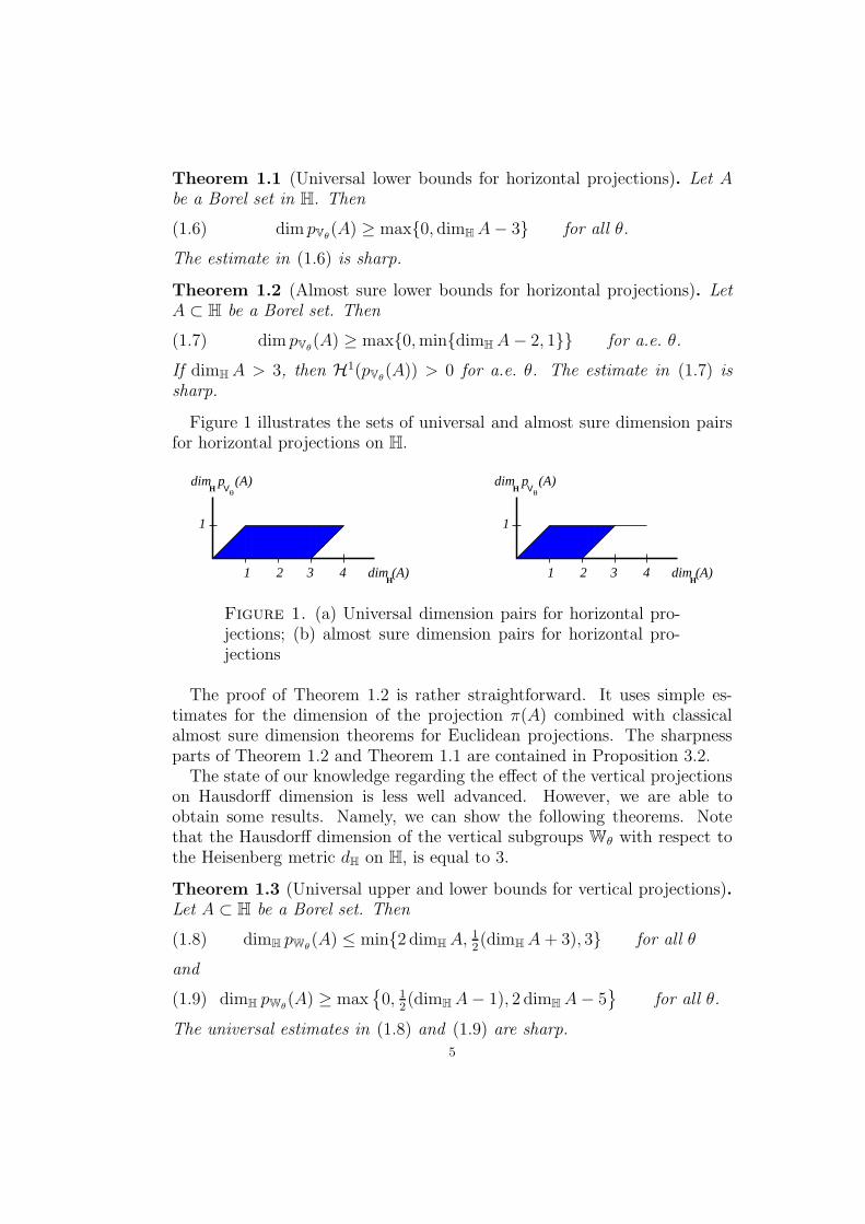
Theorem 1.1 (Universal lower bounds for horizontal projections). Let Abe a Borel set in H. Then
(1.6) dim pVθ(A) ≥ max0, dimHA− 3 for all θ.
The estimate in (1.6) is sharp.
Theorem 1.2 (Almost sure lower bounds for horizontal projections). LetA ⊂ H be a Borel set. Then
(1.7) dim pVθ(A) ≥ max0,mindimHA− 2, 1 for a.e. θ.
If dimHA > 3, then H1(pVθ(A)) > 0 for a.e. θ. The estimate in (1.7) is
sharp.
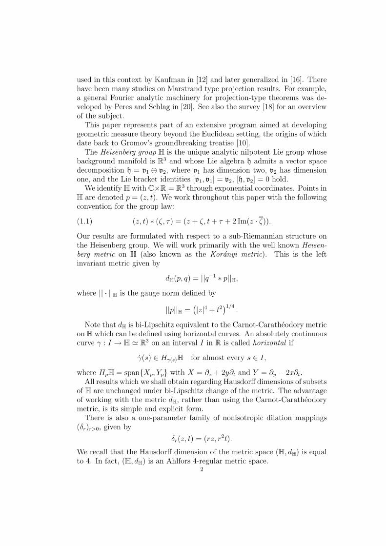
Figure 1 illustrates the sets of universal and almost sure dimension pairsfor horizontal projections on H.
1
1 2 3 4 dim (A)H
Hdim p (A)
θV
1
1 2 3 4 dim (A)H
Hdim p (A)
θV
Figure 1. (a) Universal dimension pairs for horizontal pro-jections; (b) almost sure dimension pairs for horizontal pro-jections
The proof of Theorem 1.2 is rather straightforward. It uses simple es-timates for the dimension of the projection π(A) combined with classicalalmost sure dimension theorems for Euclidean projections. The sharpnessparts of Theorem 1.2 and Theorem 1.1 are contained in Proposition 3.2.
The state of our knowledge regarding the effect of the vertical projectionson Hausdorff dimension is less well advanced. However, we are able toobtain some results. Namely, we can show the following theorems. Notethat the Hausdorff dimension of the vertical subgroups Wθ with respect tothe Heisenberg metric dH on H, is equal to 3.
Theorem 1.3 (Universal upper and lower bounds for vertical projections).Let A ⊂ H be a Borel set. Then
(1.8) dimH pWθ(A) ≤ min2 dimHA,
12(dimHA + 3), 3 for all θ
and
(1.9) dimH pWθ(A) ≥ max
0, 1
2(dimHA− 1), 2 dimH A− 5
for all θ.
The universal estimates in (1.8) and (1.9) are sharp.5

Theorem 1.4 (Almost sure lower bounds for vertical projections). Let Abe a Borel set in H. If dimHA ≤ 1, then
(1.10) dimH pWθ(A) ≥ dimHA for a.e. θ.
Consequently, for any A,
(1.11) dimH pWθ(A) ≥ maxmindimHA, 1, 2 dimH A− 5 for a.e. θ.
The estimate (1.11) is sharp when dimHA ≤ 1.
1
1 2 3 4 dim (A)H
2
3
Hdim p (A)
θW
1
1 2 3 4 dim (A)H
2
3
Hdim p (A)
Wθ
Figure 2. (a) Universal dimension pairs for vertical projec-tions; (b) almost sure dimension pairs for vertical projections(including conjectured sharp lower bound)
The sharpness statement of Theorem 1.3 is discussed in Proposition 4.10.The upper bound (1.8) is also sharp as an almost sure statement, see Propo-sition 5.3. Examples which prove the sharpness of the lower bound (1.11) inTheorem 1.4 in the case when dimH A ≤ 1 are given by subsets of the t-axis.We do not know whether the lower bound (1.11) is sharp in the case when1 < dimH A < 4 but we suspect not. We formulate the following
Conjecture 1.5. For all A ⊂ H, dimH pWθ(A) ≥ mindimHA, 3 for a.e. θ.
If dimHA > 3, then H3H(pWθ
(A)) > 0 for a.e. θ.
Proposition 6.1 and Theorem 6.3 provide partial evidence in support ofConjecture 1.5.
Figure 2 illustrates the sets of universal and almost sure dimension pairsfor vertical projections on H (including the conjectured sharp lower bound).
The lower bounds in Theorem 1.4 can be improved in case the set A isa subset of either a horizontal plane or a vertical plane. See Section 7 fordetails.
We would like to emphasize an important difference between Theorems 1.2and 1.4 and their Euclidean predecessor, see Theorem 2.3 below. Namely,for any Borel set A ⊂ Rn, the almost sure dimension of the image PV (A)under a Euclidean projection on an m-dimensional subspace V can be com-puted exactly as a function of dimE A and m. No similar formula holds in
6
the Heisenberg setting, at least for arbitrary Borel sets. Indeed, the bestresult which can be obtained is a pair of (distinct) upper and lower boundsfor the Heisenberg dimensions of the projections. We give a variety of exam-ples to demonstrate the sharpness of our estimates. Finally, let us remarkthat we do obtain an exact formula for the L1-almost sure dimension of thehorizontal projection in the low codimensional case dimH A > 3. Conjec-turally, a similar exact formula holds for the vertical projections under thesame assumption on dimH A.
We conclude this introduction with an outline of the paper. In Section2 we recall preliminary information concerning almost sure dimension the-orems in Euclidean space and the dimension comparison principle in theHeisenberg group. Section 3 treats the case of the horizontal projectionmappings and contains the proof of Theorems 1.1 and 1.2. Section 4 con-tains the proof of the universal dimension bounds for the vertical projectionmappings: Theorem 1.3. The main results of the paper concerning the al-most sure dimension theorem for vertical projections, Theorem 1.4 and therelated examples, are presented in Section 5. Since our results on almostsure dimensions of vertical projections are rather incomplete, we will dis-cuss several classes of examples where we have a better understanding ofthe behavior of the dimension of the projections. The first such class con-sists of sets with a certain degree of regularity. This is discussed in Section6. In Section 7 we sharpen the analysis of the vertical projections, obtain-ing improved dimension estimates for projections of subsets of horizontal orvertical planes. Section 8 contains remarks and open questions motivatedby this study.
1.1. Acknowledgements. Research for this paper was initiated while EDCand JTT were guests in the Mathematics Institute of the University of Bernin Fall 2009 and completed while PM was a guest of the same institute inFall 2010. The hospitality of the institute is gratefully appreciated.
2. Review of background material
2.1. Dimension and Euclidean projections. Theorems 1.2 and 1.4 areadaptations to the Heisenberg setting of classical almost sure dimensiontheorems for Euclidean projections, proved by Marstrand in the plane [15]and generalized in [16]. We briefly recall the Euclidean theorems.
Definition 2.1. Letm and n be integers with 0 < m < n. The GrassmanianG(n,m) is the space of all m-dimensional linear subspaces of Rn.
It is possible to introduce a natural measure γn,m on G(n,m). In the casem = 1 this measure is fairly simple to describe. In fact, the GrassmanianG(n, 1) coincides with the real projective space P n−1
R, and the measure in
question is the pushforward of the surface measure from Sn−1 under the7
canonical quotient map Sn−1 → P n−1R
. For instance, G(2, 1) can be identifiedwith P 1
R, or even more explicitly with the interval [0, π) (by identifying a line
through the origin in R2 with the angle θ ∈ [0, π) which it makes with thepositive x-axis). Under the latter identification, the measure in question isjust dθ. Via the canonical identification of the Grassmanians G(n,m) andG(n, n−m), we could also describe the natural measure on G(n, n−1) quiteexplicitly. However, for 2 ≤ m ≤ n − 2 the story is more complicated. Werefer to [17, §3] for the construction of the measure γn,m on G(n,m). It canbe checked that γn,m is equivariant with respect to the usual action of theorthogonal group O(n) on G(n,m).
Remark 2.2. The measure γn,m can be constructed in another manner. TheGrassmanian G(n,m) is a smooth manifold of dimension m(n−m), and isalso a metric space when equipped with the function d(V,W ) = ||PV −PW ||.Here PV : Rn → V denotes orthogonal projection from Rn onto a subspaceV , and || · || denotes the operator norm. Up to a multiplicative constant,the measure γn,m coincides with the Hausdorff measure Hm(n−m) on themetric space (G(n,m), d). This follows easily from the fact that both of themeasures in question are O(n) equivariant, and hence uniformly distributed.See Definition 3.3 and Theorem 3.4 in [17] for additional details.
Theorem 2.3 (Euclidean Projection Theorem). Let m and n be integerswith 0 < m < n and let A ⊂ Rn be a Borel set. If dimE A ≤ m, thendimE PV (A) = dimE A for γn,m-a.e. V ∈ G(n,m). If dimE A > m, thenHm(PV (A)) > 0 for γn,m-a.e. V ∈ G(n,m). In particular,
(2.1) dimE PV (A) = mindimE A,m for γn,m-a.e. V .
A Suslin set is the continuous image of a Borel set. Theorem 2.3 extendsto Suslin sets.
Frostman’s lemma is a standard tool used in the proof of lower bounds forHausdorff dimension. We denote by M(A) the collection of positive, finiteBorel regular measures supported on a set A of a metric space X.
Theorem 2.4 (Frostman’s lemma). Let A be a Borel (Suslin) subset of acomplete metric space (X, d). Suppose that there exists s > 0, µ ∈ M(A),and r0 ∈ (0,∞] so that the inequality
(2.2) µ(B(x, r)) ≤ rs
holds for all x ∈ A and 0 < r < r0. Then Hs(A) > 0. In particular,dimA ≥ s.
Conversely, if Hs(A) > 0 then there exists a measure µ ∈ M(A) so that(2.2) holds for all x ∈ A and r > 0.
See, e.g., [7, Proposition 4.2], [11] or [17, Theorem 8.17].We say that µ satisfies an upper mass bound on A with exponent s if (2.2)
holds for all x ∈ A and 0 < r < r0.8
Next, we state the energy version of Frostman’s lemma. This follows easilyfrom Theorem 2.4, see [17, Chapter 8].
Definition 2.5. Let (X, d) be a metric space and let µ ∈ M(X). For s > 0,the s-energy of µ is
Is(µ) =
∫X
∫X
d(x, y)−s dµ(x) dµ(y).
Theorem 2.6 (Energy version of Frostman’s lemma). Let A be a Borel(Suslin) subset of a complete metric space (X, d) and let s > 0 be such thatthere exists µ ∈ M(A) with Is(µ) < ∞. Then dimA ≥ s. Conversely, if Ais a Borel (Suslin) subset of a complete metric space (X, d) and s < dimA,then there exists µ ∈ M(A) with Is(µ) <∞.
2.2. Dimension comparison principle. We will make use of the recentsolution to the dimension comparison problem in H. This problem, orig-inally posed by Gromov [10, §0.6.C], asks for sharp estimates relating theEuclidean and Heisenberg measures and dimensions of subsets of H. Anearly complete answer was given by Balogh–Rickly–Serra-Cassano [3]; thestory was completed by Balogh–Tyson [4] who gave examples demonstrat-ing the sharpness of the lower bound. We state the final result, in its sharpform.
Theorem 2.7 (Dimension comparison in the Heisenberg group). Let A ⊂ H
be a set with dimE A = α ∈ [0, 3] and dimHA = β ∈ [0, 4]. Then
(2.3) maxα, 2α− 2 =: β−(α) ≤ β ≤ β+(α) := min2α, α+ 1.Moreover, for any pair (α, β) ∈ [0, 3] × [0, 4] satisfying β−(α) ≤ β ≤ β+(α),there is a compact set Aα,β ⊂ H with dimE Aα,β = α and dimHAα,β = β.
Theorem 2.7 was generalized to arbitrary Carnot groups by Balogh, Tysonand Warhurst [5].
From now on, we refer to the estimates in (2.3) as the dimension compar-ison principle for the Heisenberg group H.
We will also use the dimension comparison principle in vertical subgroupsof H. Due to the special form (1.4) of the restriction of the Koranyi metric tosuch subspaces, we obtain stronger dimension comparison estimates therein.To wit, we have
Theorem 2.8 (Dimension comparison in vertical subgroups of the Heisen-berg group). Let A ⊂ Wθ be a set contained in some vertical subgroupWθ ⊂ H, with dimE A = α ∈ [0, 2] and dimH A = β ∈ [0, 3]. Then
(2.4) maxα, 2α− 1 =: βW
− (α) ≤ β ≤ βW
+ (α) := min2α, α+ 1.Theorem 2.8 can be proved by adapting the arguments from [5].
9
2.3. Explicit formulas for horizontal and vertical projections. Wepresent explicit formulas for the projection mappings pVθ
and pWθ, and for
the distance between points in H and the corresponding distance betweentheir projections. Such formulas will be useful in the proofs of Theorems 1.2and 1.4.
Let θ ∈ [0, π) and let p = (z, t) ∈ H. We recall that the projections pVθ
and pWθare determined by the identity
(2.5) p = pWθ∗ pVθ
.
The horizontal projection pVθcoincides with the Euclidean orthogonal pro-
jection PVθ: R3 → Vθ and is given by
(2.6) pVθ(z, t) = pVθ
=(Re(e−iθz)eiθ, 0
).
The vertical projection pWθcan then be determined via (2.5) and is given
by
(2.7) pWθ(z, t) = pWθ
=(Im(e−iθz)ieiθ, t− Im(e−2iθz2)
).
Denote by p = (z, t) and q = (ζ, τ) two points in H. Observing thatIm((z− ζ)(z + ζ)) = 2 Im(zζ) and using the formula (1.1) for the group lawin H, we record the following expression for the distance between p and q:
d4H(p, q) = ||q−1 ∗ p||4
H= |z − ζ |4 + (t− τ + |z2 − ζ2| sin(ϕ1 − ϕ2))
2.(2.8)
Here we wrote ϕ1 = arg(z − ζ) and ϕ2 = arg(z + ζ).Similarly, the distance between pVθ
(p) and pVθ(q) can be expressed in the
form
dH(pVθ(p), pVθ
(q)) = ||pVθ(q)−1 ∗ pVθ
(p)||H = |z − ζ || cos(ϕ1 − θ)|.Finally, the distance between pWθ
(p) and pWθ(q) can be expressed in the
form
d4H(pWθ
(p), pWθ(q)) = ||pWθ
(q)−1 ∗ pWθ(p)||4
H
= |z − ζ |4 sin4(ϕ1 − θ) + (t− τ − |z2 − ζ2| sin(ϕ2 + ϕ1 − 2θ))2.
(2.9)
Note that the vertical projections pWθ: H → Wθ are locally 1
2-Holder con-
tinuous with respect to the Heisenberg metric. This is an easy computationinvolving the explicit formula for the projection.
3. Projections onto horizontal subspaces
In this section, we discuss the effect of horizontal projections on Borel setsin the Heisenberg group.
We begin with a lemma on the relationship between the Heisenberg di-mension of a set in H and the Euclidean dimension of its planar projection.
Lemma 3.1. For any set A ⊂ H, we have dimE π(A) ≥ dimH A− 2.10
Proof. We may assume without loss of generality that A is bounded. In fact,let us assume that |t| ≤ 1 for all points p = (z, t) ∈ A.
Let s > dimE π(A), let ε > 0, and cover the set π(A) with a family ofEuclidean balls BE(zi, ri)i so that
∑i rsi < ε. Since π : (H, dH) → (R2, dE)
is 1-Lipschitz, the fiber π−1(BE(z, r)) contains the ball BH((z, t), r) for anyt ∈ R. We can choose an absolute constant C0 > 0 and Ni ≤ C0r
−2i values
tij so that the family BH((zi, tij), C0ri)j covers the set BE(zi, ri)× [−1, 1].Then BH((zi, tij), C0ri)i,j covers the set A. Denoting by rad(B) the radiusof a ball B, we compute∑
i,j
rad(BH((zi, tij), C0ri))s+2 =
∑i
Ni(C0ri)s+2 ≤ Cs+3
0
∑i
rsi ≤ Cs+30 ε.
Letting ε→ 0 gives Hs+2H
(A) = 0 so dimHA ≤ s+2. Letting s→ dimE π(A)completes the proof.
Proof of Theorems 1.1 and 1.2. Let A ⊂ H satisfy dimHA > 2. By Lemma3.1, dimE π(A) ≥ dimHA− 2. Let us identify the one-dimensional subspaceof R2 spanned by the vector eiθ with the corresponding one-dimensionalsubspace Vθ ⊂ H. This allows us to consider the Euclidean projection mapPVθ
as a (1-Lipschitz) map from R2 to Vθ.
Applying the Euclidean Projection Theorem 2.3 to π(A) (note that π(A)is a Suslin set) and noting that pVθ
= PVθ π, we find
dim pVθ(A) = dimE PVθ
(π(A)) ≥ min1, dimE π(A) ≥ min1, dimH A− 2for a.e. θ. This proves (1.7). In the case when dimHA > 3, we use the secondpart of Theorem 2.3 to arrive at the desired conclusion H1(pVθ
(A)) > 0 fora.e. θ. Finally, for any θ, we have
dimH pVθA = dimE PVθ
(π(A)) ≥ dimE π(A) − 1 ≥ dimH A− 3.
The proof is complete.
Both the universal bounds and the almost sure bounds for dimensiondistortion by horizontal projections are sharp. We collect relevant examplesdemonstrating this in the following proposition.
Proposition 3.2. In each of the following statements, the set A is a compactsubset of H.
(a) For all 0 ≤ β ≤ 1 there exists A so that
dimHA = β and dim pVθ(A) = β for all θ.
(b) For all 1 ≤ β ≤ 4 there exists A so that
dimHA = β and dim pVθ(A) = 1 for all θ.
11

(c) For all 0 ≤ β ≤ 3 there exists A so that
dimHA = β and dim pV0(A) = 0.
If 0 ≤ β ≤ 2 we can choose A so that dim pVθ(A) = 0 for all θ.
(d) For all 3 ≤ β ≤ 4 there exists A so that
dimHA = β and dim pV0(A) = β − 3.
(e) For all 2 ≤ β ≤ 3 there exists A so that
dimH A = β and dim pVθ(A) = β − 2 for all θ.
Recall that a Borel set E is called an s-set, s ≥ 0, if 0 < Hs(E) < ∞. Abounded metric space (X, d) is said to be Ahlfors regular of dimension s ≥ 0if there exists a measure µ ∈ M(X) and a constant C ≥ 1 so that
C−1rs ≤ µ(B(x, r)) ≤ Crs
for all x ∈ X and 0 < r < diamX. If (X, d) is Ahlfors regular of dimensions, then dimX = s and µ is comparable to the Hausdorff measure Hs.
Proof. For part (a), let A0 ⊂ V0 and Aπ/2 ⊂ Vπ/2 be compact β-sets. Theset A = A0 ∪ Aπ/2 verifies the stated conditions.
To show part (b) it suffices to construct a compact set A with dimHA = βand such that π(A) is a planar set which projects onto a 1-dimensional subsetof Vθ for every θ. We consider two cases. First, assume that 1 ≤ β ≤ 3.Let S ⊂ [0, 1] be a compact (β − 1)/2-set and let A = A0 ∪ Aπ
2, where
A0 = (x, t) : 0 ≤ x ≤ 1, t ∈ S and Aπ2
= (iy, t) : 0 ≤ y ≤ 1, t ∈ S.Since the restriction of dH to any vertical subgroup is comparable with theheat metric, dimHA = 1 + 2 dimS = β. The set π(A) is the union of twoline segments which form a right angle at the origin. For θ = 0 and θ = π
2one of the two segments is projected to a single point, but the projection ofthe entire set π(A) on Vθ is 1-dimensional for every direction θ as desired.Next, assume that 3 < β ≤ 4. In this case, take the set A to be theunion of any compact set of Heisenberg Hausdorff dimension β with the set(z, 0) : |z| ≤ 1. This completes the proof for part (b).
We now turn to the proof of part (c). For the first claim, any compactβ-set A ⊂ W0 suffices. In case 0 ≤ β ≤ 2 we can choose this compact set Ato be a subset of the t-axis, in which case pVθ
(A) = (0, 0) for all θ.Next we consider part (d). We may assume that 3 < β < 4. Let S ⊂ R
be a compact set which is Ahlfors regular of dimension (β − 3), let
B0 = (iy, t) : 0 ≤ y ≤ 1, 0 ≤ t ≤ 1and let
A = p0 ∗ (x, 0) : p0 ∈ B0, x ∈ S.12
Then pV0(A) = (x, 0) : x ∈ S has dimension β − 3. It suffices to provethat dimHA ≥ β. We will use Theorem 2.4. It suffices to show that themeasure
µ(E) :=
∫S
H3H(p0 ∗ (x, 0) : p0 ∈ B0 ∩ E) dHβ−3
E (x)
has the upper mass bound (2.2) on A with exponent β. Let BH(p, r) be aball in (H, dH) centered at p = p0 ∗ (x0, 0) ∈ A with radius r.
For x ∈ S, denote by Bx the set of points of the form q ∗ (x, 0), q ∈ B0.
Lemma 3.3. If BH(p, r) ∩ Bx = ∅, then |x− x0| ≤ r and
H3H(BH(p, r) ∩ Bx) ≤ Cr3
for a constant C independent of p, r and x.
Assuming the lemma we complete the proof in this case:
µ(BH(p, r)) ≤ Cr3 · Hβ−3E ([x0 − r, x0 + r] ∩A) ≤ C ′rβ.
Hence µ satisfies the upper mass bound (2.2) on A with exponent β. ByTheorem 2.4 dimHA ≥ β.
It remains to prove the lemma. Suppose that BH(p, r) ∩ Bx = ∅. ThenBH(p, r) ⊂ BH(q, 2r) for some q ∈ BH(p, r) ∩ Bx and
H3H(BH(p, r) ∩Bx) ≤ H3
H(BH(q, 2r) ∩Bx) ≤ Cr3
since Bx lies in a vertical plane in H. Furthermore, if q = (iy, t) ∗ (x, 0) then|x − x0| ≤ r. This completes the proof of Lemma 3.3 and hence completesthe construction for part (d).
Finally, we consider part (e). It suffices to construct a compact set A ⊂ H
with dimHA = β such that π(A) is a (β − 2)-dimensional set in the planewhose dimension is preserved under PVθ
for every θ. Let S ⊂ R be a compact(β − 2)-set and let A = A0 ∪ Aπ
2, where A0 = (x, t) : x ∈ S, 0 ≤ t ≤ 1
and Aπ2
= (iy, t) : y ∈ S, 0 ≤ t ≤ 1. Since the restriction of dH toany vertical subgroup is comparable with the heat metric, we have thatdimHA = dimS + 2 = β. Moreover, dimE π(A) = dimE S = β − 2. Thedimension of the set π(A0) is preserved under PVθ
except for θ = π2, in which
case π(A0) is projected to a single point. An analogous statement holds forπ(Aπ
2) and the exceptional direction θ = 0. Altogether, it follows for all θ
that dim pVθ(A) = dimPVθ
(π(A)) = β − 2.The proof of Proposition 3.2 is complete.
4. Universal bounds for vertical projections
In this section, we start to discuss the effect of vertical projections on thedimensions of Borel sets in the Heisenberg group. Our purpose is to proveTheorem 1.3.
13
We recall that the projection map pWθfrom H to the vertical subgroup
Wθ is given by
(4.1) pWθ(z, t) =
(Im(e−iθz)ieiθ, t− Im(e−2iθz2)
).
In contrast with the Euclidean case, this map is not Lipschitz continuousand hence does not a priori decrease dimension. Indeed, there are caseswhen this map increases dimension. Yet, there is still a certain control onthe upper dimension bound coming from the local 1
2-Holder continuity of
pWθwith respect to dH. Thus, for an arbitrary subset A of H and for all θ,
we have
(4.2) dimH pWθ(A) ≤ 2 dimH A.
Example 4.1. Let A = (1 + i)s, 0) : s ∈ [0, 1] ⊂ H be a one-dimensionalhorizontal line segment. The projection of A by the map pW0 is the graphof a parabola contained in the vertical subspace W0. Thus pW0(A) is a non-horizontal smooth curve and so has Hausdorff dimension equal to two. Thisshows that for 1-dimensional sets the upper bound (4.2) cannot be improved.
The proof of Theorem 1.3 is given in a series of propositions. Our firststatement indicates the universal upper bounds which hold for the dimen-sions of vertical projections. Within a certain dimension range, the trivialupper bound given in (4.2) can be improved.
Proposition 4.2. Let A ⊂ H be any Borel set. Then
(4.3) dimH pWθ(A) ≤ min2 dimHA,
12(dimHA + 3), 3
for every θ.
The cases 3 < dimH A ≤ 4 and 0 ≤ dimH A < 1 are trivial. The latterfollows from the local 1
2-Holder continuity of pWθ
. We will focus on theremaining case 1 ≤ dimHA ≤ 3. The proof in this situation is more involvedand uses a covering argument.
Proposition 4.3. Let A be a Borel subset of H with dimHA ∈ [1, 3]. Forall θ ∈ [0, π) we have
(4.4) dimH pWθ(A) ≤ 1
2(dimHA+ 3).
The proof of this proposition is based on two preliminary results. Lemma4.5, which describes the image of Heisenberg balls under vertical projections,and Lemma 4.6, which explains how this set can be covered efficiently byballs in the vertical plane. This allows us to find good covers for pWθ
(A)which then yields the desired upper bound for the Hausdorff dimension.
If not otherwise mentioned, we will in the following always identify thevertical plane Wθ with R2 as described in (1.3). A point p = (αieiθ, τ) inWθ will be written in coordinates as (α, τ).
14
Let 0 < r < 1 and x0 ∈ R. First, we describe the vertical projection indirection θ ∈ [0, π) of a ball BH(p0, r) with center p0 = (x0, 0) on the x-axis.We prove that there is a “core curve” γx0,r
θ such that the image of the ballunder pWθ
lies in a small Euclidean neighborhood of the projected curve.For the following steps of the proof it will be essential to control the size ofthis neighborhood independently of the direction θ. This can be achieved ifone uses a different curve depending on whether θ is close to π
2, or it is close
to 0 or π.
Definition 4.4. The core curve γx0,rθ related to x0 ∈ R and 0 < r < 1 is a
subset of H, given by
γx0,rθ :=
(x0 + iy,−2x0y) : y ∈ [−2r, 2r], if θ ∈ [0, π4] ∪ [3π
4, π),
(x0 + x, 0) : x ∈ [−2r, 2r], if θ ∈ (π4, 3π
4).
A direct computation shows that for each θ ∈ [0, π), x0 ∈ R and 0 < r < 1,the image under pWθ
of the corresponding core curve γx0,rθ is the graph of a
linear or quadratic function fx0,rθ over an interval Ix0,r
θ .
Lemma 4.5. For all θ ∈ [0, π), p0 = (x0, 0) with x0 ∈ R, and 0 < r < 1,we have
pWθ(BH(p0, r)) ⊆ NE(pWθ
(γx0,rθ ), 5r2),
where the expression on the right denotes the Euclidean 5r2-neighborhood ofpWθ
(γx0,rθ ).
More precisely,
pWθ(BH(p0, r)) ⊆(4.5)
(α, τ) ∈ R2 : α ∈ Ix0,r
θ , fx0,rθ (α) − 5r2 ≤ τ ≤ fx0,r
θ (α) + 5r2.Proof of Lemma 4.5. We discuss the proof for the case θ ∈ (0, π
4]. The other
cases can be treated similarly, using the appropriate core curve.For an arbitrary point (x′ + iy′, t′) in the ball BH(p0, r), one finds
(4.6) |x′ − x0| ≤ r, |y′| ≤ r and |t′ + 2x0y′| ≤ r2.
The projection is given by
pWθ(x′ + iy′, t′) = (−x′ sin θ + y′ cos θ, t′ + (x′2 − y′2) sin 2θ − 2x′y′ cos 2θ)
=: (α′, τ ′).
For points on the core curve, (x0 + iy,−2x0y) ∈ γx0,rθ , we have
pWθ(x0 + iy,−2x0y)
= (−x0 sin θ + y cos θ,−2x0y + (x20 − y2) sin 2θ − 2x0y cos 2θ)
=: (α, τ).
15
Thus, as a subset of R2, the set pWθ(γx0,rθ ) coincides with the graph of the
function
(4.7) fx0,rθ (α) = −2 tan θ(α + x0
sin θ)2 + x2
0(2
sin θ cos θ− 2 tan θ)
over the interval
Ix0,rθ = [−x0 sin θ − 2r cos θ,−x0 sin θ + 2r cos θ].
The goal is now to find a point in pWθ(γx0,rθ ) which lies close to the point
pWθ(x′ + iy′, t′). To this end, let
(4.8) y := y′ − (x′ − x0) tan θ
and note that
|y| ≤ |y′| + |x′ − x0|| tan θ| ≤ (1 + | tan θ|)r ≤ 2r.
It follows (x0 + iy,−2x0y) ∈ γx0,rθ . We claim that the Euclidean distance
between the points pWθ(x0 + iy,−2x0y) and pWθ
(x′ + iy′, t′) is at most 5r2.First, we observe
|α− α′| =|(x′ − x0) sin θ + (y − y′) cos θ|=|(x′ − x0) sin θ − (x′ − x0) tan θ cos θ|=0
for y as in (4.8).Second, we compute
|τ − τ ′| = | − 2x0y − t′ + (x20 − y2 − x′2 + y′2) sin 2θ − 2 cos 2θ(x0y − x′y′)|.
Inserting y from (4.8) and using trigonometric relations yields
|τ − τ ′| =| − 2x0y′ − t′ + 2x0(x
′ − x0) tan θ
+ 2 sin θ cos θ(x20 + 2y′(x′ − x0) tan θ − (x′ − x0)
2 tan2 θ − x′2)
− 2(cos2 θ − sin2 θ)(x0y′ − x0(x
′ − x0) tan θ − x′y′)|=| − (t′ + 2x0y
′) + 2x0(x′ − x0) sin θ cos θ + 2x′(x0 − x′) sin θ cos θ
− 2y′(x0 − x′) − 2 sin3 θcos θ
(x′ − x0)2|
=| − (t′ + 2x0y′) − 2(x0 − x′)2 sin θ cos θ − 2y′(x0 − x′)
− 2 sin3 θcos θ
(x′ − x0)2|
=| − (t′ + 2x0y′) − 2(x0 − x′)2 tan θ − 2y′(x0 − x′)|.
Hence, from (4.6) it follows,
|τ − τ ′| ≤ |t′ + 2x0y| + 2| tan θ||x0 − x′|2 + 2|y′||x0 − x′|≤ (1 + 2| tan θ| + 2)r2.
For θ ∈ (0, π4] this yields
√(α− α′)2 + (τ − τ ′)2 ≤ 5r2 which concludes the
proof in this case. The proof for θ ∈ [3π4, π) is very similar. We employ again
16
the formula (4.7). For θ = 0 we have to consider a linear function instead ofthe quadratic function (4.7). The case θ ∈ (π
4, 3π
4) can be treated similarly,
starting from a core curve of the second type.
Lemma 4.6. Let θ ∈ [0, π) and R > 0. There exist constants c1 > 0 andc2 = c2(R) > 0 such that for all 0 < r < 1, z0 = |z0|eiθ0 ∈ C with |z0| ≤ Rand t0 ∈ R, the set
pWθ(BH((z0, t0), r))
can be covered by M balls BWθ(pj, c1r
2) := BH(pj, c1r2)∩Wθ, j ∈ 1, . . . ,M,
with M ≤ c2r3
.
Proof. Since the restriction of the Heisenberg metric to the vertical plane Wθ
is comparable to the parabolic heat metric on R2, there exists a constant
c1 > 0 such that
R(p, r2) := (α, τ) ∈ R2 : |α− α′| ≤ r2, |τ − τ ′| ≤ r4 ⊆ BWθ
(p, c1r2)
for all p = (α′, τ ′) ∈ Wθ and r ≥ 0. It is therefore enough to construct acover by rectangles R(pj , r
2), j ∈ 1, . . . ,M.Moreover, it suffices to prove the result for balls centered on the x-axis, i.e.,
for balls BH((z0, t0), r) with z0 = x0 ∈ R and t0 = 0. Indeed, an arbitraryball BH((z0, t0), r) can be obtained from BH((|z0|, 0), r) by a (Euclidean)vertical translation to height t0 and a rotation about the t-axis with rotationangle θ0. Then, as a subset of R2, the image pWθ
(BH((z0, t0), r)) coincideswith a vertical translation of pWθ−θ0
(BH((|z0|, 0), r)).
Let us consider a ball with radius r < 1, centered at a point p0 = (x0, 0)with x0 ∈ R, |x0| < R. The goal is to cover the set
Sθ(x0, r) := (α, τ) ∈ R2 : α ∈ Ix0,r
θ , fx0,rθ (α) − 5r2 ≤ τ ≤ fx0,r
θ (α) + 5r2⊆ Wθ
which, by Lemma 4.5, contains the image of BH(p0, r) under pWθ, efficiently
by rectangles R(pj , r2), j ∈ 1, . . . ,M.
Let us assume that fx0,rθ is defined on the entire real line. For given θ and
x0, we fix a particular point
α0 :=
− x0
sin θ, if θ ∈ (0, π
4] ∪ [3π
4, π),
0, else.
In the case where fx0,rθ is a quadratic function, it has an extremal point at
α0. This is shown in the proof of Lemma 4.5 for the case θ ∈ (0, π4]∪ [3π
4, π).
We write
(Ix0,rθ )k := [α0 + kr2, α0 + (k + 1)r2).
It can be checked that the interval Ix0,rθ has length at most 4r (this is done
explicitly in the proof of Lemma 4.5 for the case θ ∈ (0, π4]), whereas each
17
interval of the form (Ix0,rθ )k has length r2. It follows that Ix0,r
θ has nonemptyintersection with at most
(4.9) N ≤ 6
r
of the disjoint intervals (Ix0,rθ )k. Let k be such that Ix0,r
θ ∩ (Ix0,rθ )k = ∅.
Consider now the portion of Sθ(x0, r) which lies above the interval (Ix0,rθ )k,
more precisely,
(α, τ) ∈ Sθ(x0, r) : α ∈ (Ix0,rθ )k.
In order to see how many rectangles R(pj, r2) we need to cover this set, we
have to estimate its vertical height. A direct computation for the severalpossible cases shows that there exists a constant c0 = c0(R) such that foreach k ∈ Z with Ix0,r
θ ∩ (Ix0,rθ )k = ∅ there is an interval (Jx0,r
θ )k of lengthc0r
2 with
(4.10) (α, τ) ∈ Sθ(x0, r) : α ∈ (Ix0,rθ )k ⊆ (Ix0,r
θ )k × (Jx0,rθ )k.
Hence, because of (4.5) and (4.10), there exists an integer N ′ ∈ N and points
pk,l = (αk,l, τk,l), l ∈ 1, . . . , N ′in the vertical plane Wθ with
(4.11) N ′ ≤ c0 + 1
r2
such that
pWθ(BH((x0, 0), r)) ∩ ((Ix0,r
θ )k × R) ⊆N ′⋃l=1
R(pk,l, r2).
From (4.9) and (4.11) it follows that the image pWθ(BH((x0, 0), r)) can be
covered by
M := N ·N ′ ≤ 6(c0 + 1)
r3
rectangles R(pj , r2) = R(pk,l, r
2). Since each of these rectangles is containedin a ball BW(pj , c1r
2), this concludes the proof of Lemma 4.6.
Proof of Proposition 4.3. We may without loss of generality assume that theset A is bounded. We denote its Hausdorff dimension by dimHA = s ∈ [1, 3].Then we have Hs+ε
H(A) = 0 for all ε > 0 and thus, for each ε > 0,
(HH)s+εδ (A) = 0 for all δ > 0.
Hence, for all ε > 0 and 0 < δ < 1, there exists a countable collection ofballs
BH(pi, ri), i ∈ N, ri ≤ δ18

with
(4.12) A ⊆⋃i∈N
BH(pi, ri),
∞∑i=1
rs+2εi < δ.
We write pi = (zi, ti) = (|zi|eiθ0,i, ti). Since the set A is bounded, we mayassume that there exists R > 0 such that |zi| ≤ R for all i ∈ N.
Fix now θ ∈ [0, π). It follows from Lemma 4.6 that there exist c1, c2 > 0(independent of pi and ri), constants Mi with Mi ≤ c2
r3i, and points pi,j, i ∈ N
and j ∈ 1, . . . ,Mi such that
(4.13) pWθ(A) ⊆
⋃i∈N
Mi⋃j=1
BWθ(pi,j, c1r
2i ).
For σ ≥ 0, notice that
∑i,j
diam(BWθ(pi,j, c1r
2i ))
σ+ε =∑i∈N
Mi∑j=1
(2c1r2i )σ+ε =
∑i∈N
Mi(2c1)σ+εr2σ+2ε
i
≤ (2c1)σ+εc2
∑i∈N
r(2σ−3)+2εi .
Now if σ is chosen such that 2σ − 3 = s, i.e.,
σ =1
2(s+ 3) =
1
2(dimH A+ 3),
it follows
(4.14)∑i,j
diam(BWθ(pi,j, c1r
2i ))
σ+ε < (2c1)σ+εc2δ.
From (4.13) and (4.14), we conclude that
(HH)σ+ε2c1δ2
(pWθ(A)) ≤ (2c1)
σ+εc2δ.
Letting δ tend to zero yields
Hσ+εH
(pWθ(A)) = 0
and thus,
dimH pWθ(A) ≤ σ =
1
2(dimHA+ 3),
as desired. This concludes the proof of Proposition 4.3. Next, we discuss universal lower dimension bounds for vertical projections.
We will prove two propositions. Proposition 4.7 is the vertical analog ofLemma 3.1. Observe that the failure of the vertical projection to be Lipschitzresurfaces in the proof of this result; see (4.15). Proposition 4.9 uses a slicingtheorem for dimensions of intersections of sets with planes in Euclidean spacetogether with the dimension comparison principle. Taken together, these twopropositions establish the universal lower bounds in Theorem 1.3.
19

Proposition 4.7. Let A ⊂ H be Borel with dimHA ≥ 1. Then
dimH pWθ(A) ≥ 1
2(dimH A− 1)
for every θ.
In the proof, we use the following elementary estimate whose proof weomit. Compare Lemma 4.4 in [9].
Lemma 4.8. There exists an absolute constant C > 0 so that
||a−1 ∗ b ∗ a||4H≤ ||b||4
H+ C||b||2
H
whenever a and b are points in H with ||a||H ≤ 1 and ||b||H ≤ 1.
Proof of Proposition 4.7. We may assume without loss of generality that Ais bounded. In fact, let us assume that |z| ≤ 1 for all points p = (z, t) ∈ A.
Fix θ ∈ [0, π), let s > dimH pWθ(A), let ε > 0, and cover the set pWθ
(A)with a family of Heisenberg balls BH((zi, ti), ri)i so that
∑i rsi < ε.
Claim: We can choose C0 > 0 and Ni ≤ C0r−1/2i values (zij , tij) con-
tained in the fiber p−1Wθ
(zi, ti) so that the family BH((zij, tij), C0√ri)j covers
p−1Wθ
(BH((zi, ti), ri)).
To prove the claim, it suffices to prove that
(4.15) p−1Wθ
(BH(q, r) ∩ Wθ) ∩BH((0, 0), 1) ⊂ NH(q ∗ Vθ, C√r)
for some constant C > 0, whenever q ∈ Wθ and 0 < r ≤ 1. Here NH(S, δ)denotes the δ-neighborhood of a set S ⊂ H in the metric dH, that is,NH(S, δ) =
⋃s∈S BH(s, δ).
The inclusion in (4.15) is a consequence of the following statement:
For all q′ ∈ Wθ so that dH(q, q′) ≤ r and for all p′ ∈ Vθ so that||p′||H ≤ 1, there exists p ∈ Vθ so that dH(q′∗p′, q∗p) ≤ C
√r.
To establish this statement, choose p = p′. Then
dH(q′ ∗ p′, q ∗ p)4 = ||p−1 ∗ (q−1 ∗ q′) ∗ p||4H≤ dH(q, q′)4 + CdH(q, q′)2
by Lemma 4.8. Since dH(q, q′) ≤ r by assumption and r ≤ 1, we concludethat
dH(q′ ∗ p′, q ∗ p)4 ≤ Cr2
which finishes the proof of the claim.
With the claim in hand, the rest of the proof of Proposition 4.7 proceedsexactly as for its horizontal counterpart. The family BH((zij , tij), C0
√ri)i,j
20
covers the set A and we compute∑i,j
rad(BH((zij , tij), C0
√ri))
2s+1 =∑i
Ni(C0
√ri)
2s+1
≤ C2s+20
∑i
rsi ≤ C2s+20 ε.
Letting ε → 0 gives H2s+1H
(A) = 0 so dimHA ≤ 2s + 1. Letting s tend todimH pWθ
(A) completes the proof. Proposition 4.9. Let A ⊂ H be Borel with dimHA ≥ 3. Then
dimH pWθ(A) ≥ 2 dimH A− 5 for every θ.
Proof. It suffices to assume that dimHA > 3. By the dimension comparisonprinciple,
dimE A ≥ dimHA− 1 > 2.
Let 0 < ε < dimH A − 3. According to the classical Euclidean intersectiontheorem (see Theorem 10.10 in [17]), there exists a plane Π in R
3 for which
dimE(A ∩ Π) ≥ dimE A− 1 − ε ≥ dimH A− 2 − ε > 1.
Furthermore, we may assume that Π is not a vertical plane, i.e., Π is at-graph: the graph of a function u : C → R. Let us write
Π = (z, t) : t = u(z) := 2 Re(az) + bfor some a ∈ C and b ∈ R. Consider the map F : R2 → R2 given as thecomposition of the graph map id⊗u, the vertical projection pWθ
, and thecoordinate chart ϕWθ
(see (1.3)). Written in complex notation,
F (z) = (Im(e−iθz), 2 Re(az) + b− Im(e−2iθz2)).
The Jacobian determinant of F is given by
detDF = 2 Im(e−iθ(z − ia))
and the restriction of pWθto (z, u(z)) ∈ Π : detDF (z) = 0 is locally
bi-Lipschitz. Observe that
γ = (z, u(z)) ∈ Π : detDF (z) = 0is a line. Since dimE(A ∩ Π) > 1, dimE(A ∩ (Π \ γ)) = dimE(A ∩ Π) and itfollows that
dimE pWθ(A) ≥ dimE pWθ
(A ∩ (Π \ γ))(4.16)
= dimE(A ∩ (Π \ γ)) = dimE(A ∩ Π) ≥ dimHA− 2 − ε.
To complete the proof, we use the dimension comparison principle againto switch back from the Euclidean dimension of the projected set to its
21
Heisenberg dimension. Since pWθ(A) is contained in Wθ, we can use the im-
proved lower dimension comparison bound from Theorem 2.8. Using (4.16)we obtain
dimH pWθ(A) ≥ βW
− (dimE pWθ(A)) ≥ βW
− (dimH A− 2 − ε),
and thus, letting ε tend to zero,
dimH pWθ(A) ≥ 2 dimHA− 5,
as asserted in the statement. The proof is complete.
The result of Theorem 1.3 follows by combining Proposition 4.2, 4.7 and4.9.
We now turn to the proof of the sharpness statement of Theorem 1.3.
Proposition 4.10. In each of the following statements, the set A is a com-pact subset of H.
(a) For all 0 ≤ β ≤ 1 there exists A so that
dimHA = β and dimHpW0(A) = 0.
(b) For all 1 ≤ β ≤ 3 there exists A so that
dimHA = β and dimH pW0(A) = (β − 1)/2.
(c) For all 3 ≤ β ≤ 4 there exists A so that
dimH A = β and dimH pW0(A) = 2β − 5.
(d) For all 0 ≤ β ≤ 1 there exists A so that
dimH A = β and dimH pW0(A) = 2β.
(e) For all 1 ≤ β ≤ 3 there exists A so that
dimH A = β and dimH pW0(A) =1
2(β + 3).
(f) For all 3 ≤ β ≤ 4 there exists A so that
dimHA = β and dimH pW0(A) = 3.
Proof of Proposition 4.10. For a proof of the statements (d), (e) and (f), i.e.for the sharpness of the upper dimension bounds, see the proof of Proposition5.3, where sets are constructed for which the corresponding dimension valueshold for all directions θ, and not merely for θ = 0. In the following, wediscuss the sharpness of the lower dimension bound, i.e., the cases (a), (b)and (c).
Assume that 0 ≤ β ≤ 1. Let A ⊂ V0 be a compact β-set. Then the setpW0(A) = (0, 0) is zero-dimensional. This gives an example of a set Asatisfying (a).
22
Examples for (b) and (c) are based on the following special case (β = 3),which we describe first. Let B0 = (iy, 0) : y ∈ R be the y axis and let
(4.17) A0 = p−1W0
(B0) = (x+ iy, 2xy) : x, y ∈ R.Then dimH B0 = 1, while dimHA0 = 3.
Next, assume that 1 < β < 3; we construct a set A satisfying (b). Thedesired set is constructed as a subset of the set A0 defined in (4.17). LetS ⊂ R be a compact Ahlfors regular set of dimension (β−1)/2 and considerthe set
A = p−1W0
((iy, 0) : y ∈ S).Clearly dimH pW0(A) = dimE pW0(A) = (β − 1)/2. By Theorem 1.3,
12(dimH A− 1) ≤ dimH pW0(A)
so it suffices to verify that dimH A ≥ β. Again we will appeal to Theorem2.4; the details are similar to those in the proof of Proposition 3.2(d).
Define a set function µ on A as follows:
µ(E) =
∫S
H1H(E ∩ Ly) dH(β−1)/2
E (y), for Borel sets E ⊆ A,
where Ly := p−1W0
(iy, 0). Let BH(p, r) be a ball in (H, dH) centered at p ∈ Awith radius r. Write p = (x0 + iy0, 2x0y0) for some y0 ∈ S and x0 ∈ R.
Lemma 4.11. If BH(p, r) ∩ Ly = ∅, then |y − y0| ≤ r2 and
H1H(BH(p, r) ∩ Ly) ≤ Cr,
for a constant C independent of p, r and y.
Assuming the lemma we complete the proof in this case:
µ(BH(p, r)) ≤ Cr · H(β−1)/2E (y : BH(p, r) ∩ Ly = ∅)
≤ Cr · H(β−1)/2E ([y0 − r2, y0 + r2] ∩A) ≤ C ′rβ
for C ′ > 0 independent of p and r. Hence µ satisfies the upper mass bound(2.2) on A with exponent β. By Theorem 2.4, dimH A ≥ β.
It remains to prove the lemma. Suppose that BH(p, r) ∩ Ly = ∅. ThenBH(p, r) ⊂ BH(q, 2r) for some q ∈ BH(p, r) ∩ Ly and
H1H(BH(p, r) ∩ Ly) ≤ H1
H(BH(q, 2r) ∩ Ly) ≤ Cr
since Ly is a horizontal line. Furthermore, if q = (x+ iy, 2xy) then
p−1 ∗ q = ((x− x0) + i(y − y0), 2(x+ x0)(y − y0)).
Since dH(p, q) ≤ r we conclude
|x− x0| ≤ r and |2(x+ x0)(y − y0)| ≤ r2.23
We may restrict to the subset of A consisting of points (x+ iy, t) for which|x| ≥ 1 and consider only radii r < 1. Then
|x+ x0| ≥ 2|x| − |x− x0| ≥ 2 − r > 1
and so|y − y0| ≤ Cr2.
This completes the proof of Lemma 4.11 and ends the construction whenβ ∈ [1, 3].
Finally, assume that 3 < β ≤ 4. The desired set in this case is constructedas a union of a collection of vertical translates of the set A0 defined in (4.17).Let S ⊂ R be a compact Ahlfors regular set of dimension β − 3 and let
A =⋃s∈S
τ(0,s)(A0),
where τq : H → H, τq(p) = q ∗ p, denotes left translation by q ∈ H. ThenA ⊂ H is compact and pW0(A) ⊃ (iy, s) : y ∈ [0, 1], s ∈ S, whence
dimH pW0(A) ≥ 1 + 2(β − 3) = 2β − 5.
By Theorem 1.3, 2 dimHA − 5 ≤ dimH pW0(A), so it suffices to verify thatdimHA ≥ β. Define a set function µ on A by setting
µ(E) =
∫S
H3H(E ∩ Σs) dHβ−3
E (s), for Borel sets E ⊆ A,
where Σs = τ(0,s)(A0). Let BH(p, r) be a ball in (H, dH) centered at p ∈ Awith radius r. Write p = (x0+iy0, 2x0y0+s0) for some s0 ∈ S and x0, y0 ∈ R.Then p ∈ Σs.
Lemma 4.12. If BH(p, r) ∩ Σs = ∅, then |s− s0| ≤ Cr and
H3H(BH(p, r) ∩ Σs) Cr3.
Assuming the lemma we complete the proof in this case:
µ(BH(p, r)) ≤ Cr3 · Hβ−3E (s : BH(p, r) ∩ Σs = ∅)
≤ Cr3 · Hβ−3E ([s0 − r, s0 + r] ∩ A) ≤ Crβ.
Hence µ satisfies the upper mass bound (2.2) on A with exponent β. ByTheorem 2.4, dimHA ≥ β.
It remains to prove the lemma. Suppose that BH(p, r) ∩ Σs = ∅. ThenBH(p, r) ⊂ BH(q, 2r) for some q ∈ BH(p, r) ∩ Σs and
H3H(BH(p, r) ∩ Σs) ≤ H3
H(BH(q, 2r) ∩ Σs) ≤ Cr3
since Σs is a smooth submanifold. Furthermore, if q = (x+ iy, 2xy+ s) then
p−1 ∗ q = ((x− x0) + i(y − y0), (s− s0) + 2(x+ x0)(y − y0)).
Since dH(p, q) ≤ r we conclude
|y − y0| ≤ r and |(s− s0) + 2(x+ x0)(y − y0)| ≤ r2
24

and so
|s− s0| ≤ r2 + C|y − y0| ≤ Cr.
This completes the proof of Lemma 4.12 and ends the construction whenβ ∈ [3, 4].
5. Almost sure bounds for vertical projections
The goal of this section is to prove an almost sure lower bound for verticalprojections (Theorem 1.4) and to verify that the given universal upper boundis sharp even as an almost sure statement.
The arguments concerning the lower bound go along the lines of the proofof the corresponding Euclidean result. However, it is considerably moredifficult to establish the integrability of certain functions given in terms ofthe Heisenberg distance between projected points and the proof works onlyfor a restricted range of dimensions, namely, dimHA ≤ 1.
Here is the main proposition of this section.
Proposition 5.1. Let A ⊂ H be a Borel set with dimH A ≤ 1. ThendimH pWθ
(A) ≥ dimHA for a.e. θ.
Corollary 5.2. Let A ⊂ H be a Borel set. Then
dimH pWθ(A) ≥ mindimH A, 1 for a.e. θ.
To prove the corollary, let A be a Borel subset of H with dimHA > 1 andchoose a subset B ⊂ A with dimH B = 1. For almost every parameter θ, wehave dimH pWθ
(A) ≥ dimH pWθ(B) ≥ dimH B = 1.
Proof of Proposition 5.1. Fix 0 < σ < dimH A. By Theorem 2.6, there existsµ ∈ M(A) with
Iσ(µ) =
∫A
∫A
dH(p, q)−σ dµ(p) dµ(q) <∞.
Using this measure, we will define a family of measures µθθ∈[0,π) so thatµθ ∈ M(pWθ
(A)) and
(5.1)
∫ π
0
Iσ(µθ) dθ <∞.
Once this done, the proof is finished by another appeal to Theorem 2.6 (sincethe integrand of (5.1) must be finite for almost every θ) and by taking thelimit as σ increases to dimHA.
It remains to construct the measures µθ and verify (5.1). Consider thepushforward measure µθ := (pWθ
)µ defined by
(pWθ)µ(E) = µ(p−1
Wθ(E)).
25

It is not hard to see that µθ is in M(pWθ(A)). By Fubini’s theorem and the
definition of the pushforward measure, the integral in (5.1) is equal to
(5.2)
∫A
∫A
∫ π
0
dH(pWθ(p), pWθ
(q))−σ dθ dµ(p) dµ(q).
We claim that the quantity in (5.2) is bounded above by an absolute constantmultiple of Iσ(µ), i.e.,∫
A
∫A
∫ π
0
dH(pWθ(p), pWθ
(q))−σ dθ dµ(p) dµ(q)(5.3)
≤ C
∫A
∫A
dH(p, q)−σ dµ(p) dµ(q).
Unlike the Euclidean case, the distance dH(pWθ(p), pWθ
(q)) is not related tothe distance dH(p, q) in any simple way. This means that we are not ableto prove (5.3) by bounding the inner integral pointwise by dH(p, q)−σ as inthe Euclidean case. The main technical difficulties in the proof lie in theverification of (5.3).
In order to prove (5.3), we split the domain of integration A×A into twopieces, according to the two terms which appear in the formula (2.8) for theHeisenberg distance. Let
A1 := (p, q) ∈ A×A : |z − ζ |2 ≥ ∣∣t− τ + |z2 − ζ2| sin(ϕ1 − ϕ2)∣∣
and
A2 := (p, q) ∈ A×A : |z − ζ |2 < ∣∣t− τ + |z2 − ζ2| sin(ϕ1 − ϕ2)∣∣.
First, suppose that (p, q) ∈ A1. We observe the following distance esti-mates in this case:
dH(p, q)4 ≤ 2|z− ζ |4 and dH(pWθ(p), pWθ
(q))4 ≥ |z− ζ |4 sin4(ϕ1 − θ).
Then∫ π
0
dH(pWθ(p), pWθ
(q))−σ dθ ≤ |z − ζ |−σ∫ π
0
dθ
| sin(ϕ1 − θ)|σ ≤ C1dH(p, q)−σ,
where C1 = 2σ/4∫ π0| sin θ|−σ dθ < ∞. Note that in this case we use the
assumption σ < 1, and also that the constant C1 is independent of p and q.Next, suppose that (p, q) ∈ A2. Let us introduce the abbreviating notation
a := |z2 − ζ2|, b := t− τ, and ϕ0 := ϕ2 − ϕ1.
Observe that the condition (p, q) ∈ A2 implies that either b is nonzero, orthat both a and sinϕ0 are nonzero. We also have
dH(p, q)4 ≤ 2(b+ a sinϕ0)2
and
dH(pWθ(p), pWθ
(q))4 ≥ (b− a sin(ϕ0 + 2ϕ1 − 2θ))2.26
Hence
∫ π
0
dH(pWθ(p), pWθ
(q))−σ dθ ≤∫ π
0
|b− a sin(ϕ0 + 2ϕ1 − 2θ)|−σ/2 dθ
=1
2
∫ 2π
0
|b+ a sin θ|−σ/2 dθ
and
dH(p, q)−σ ≥ 2−σ/4 |b+ a sinϕ0|−σ/2,
so it suffices to find a constant C2 independent of a, b and ϕ0 for which
(5.4)
∫ 2π
0
dθ
|b+ a sin θ|σ/2 ≤ C2
|b+ a sinϕ0|σ/2
whenever either b = 0 or a sinϕ0 = 0.We finish the proof by verifying (5.4) for some explicit constant C2. If
a = 0, then (5.4) is satisfied for C2 = 2π, so assume a = 0. Then (5.4) isequivalent to
(5.5)
∫ 2π
0
dθ
|r + sin θ|σ/2 ≤ C2
|r + sinϕ0|σ/2
where r = b/a. By a change of variables, we may assume without loss ofgenerality that r ≥ 0. Observe that (5.5) is implied by
(5.6)
∫ 2π
0
dθ
|r + sin θ|σ/2 ≤ C2
(1 + r)σ/2,
so we are reduced to verifying (5.6).Consider the function
g(r) := (1 + r)σ/2∫ 2π
0
dθ
|r + sin θ|σ/2 .
A straightforward computation shows that g is monotone decreasing on theinterval [1,∞), with g(1) = 2σ/2
∫ 2π
0(1 + sin θ)−σ/2 dθ which is finite since
σ < 1. Suppose that 0 ≤ r < 1 and write r = sinψ for an appropriate ψ.To obtain a bound which is uniform in ψ, we use a trigonometric identity,
27

the Cauchy–Schwarz inequality and change of variables to obtain
g(sinψ) =
∫ 2π
0
(1 + sinψ
| sinψ + sin θ|)σ/2
dθ
=
∫ 2π
0
(1 + sinψ
|2 sin(ψ+θ2
) cos(ψ−θ2
)|
)σ/2
dθ
≤∫ 2π
0
| sin(ψ+θ2
)|−σ/2| cos(ψ−θ2
)|−σ/2 dθ
≤(∫ 2π
0
| sin(ψ+θ2
)|−σ dθ
)1/2(∫ 2π
0
| cos(ψ−θ2
)|−σ dθ
)1/2
= 2
∫ π
0
| sin θ|−σ dθ.
The latter integral is finite since σ < 1. This completes the proof.
The lower bound in Theorem 1.4 follows by combining Proposition 4.7,Proposition 4.9 and Corollary 5.2. The almost sure upper bound for thevertical projections is the same as the universal upper bound which wasproved in Proposition 4.2, and this bound is sharp.
Proposition 5.3. In each of the following statements, the set A is a compactsubset of H.
(a) For all 0 ≤ β ≤ 1 there exists A such that
dimHA = β and dimH pWθ(A) = 2β for all θ.
(b) For all 1 < β < 3 there exists A such that
dimHA = β and dimH pWθ(A) =
1
2(β + 3) for all θ.
(c) For all 3 ≤ β ≤ 4 there exists A such that
dimH A = β and dimH pWθ(A) = 3 for all θ.
Proof. First, we construct a set A satisfying (a) for every θ. Let A ⊂ V0 bea compact β-set. Then pWθ
(A) has Heisenberg Hausdorff dimension 2β forevery θ = 0. Compare Example 4.1. To construct an example which worksfor every value of θ, let A be the union of two compact β-sets, one containedin V0 and one contained in Vπ/2.
It is not hard to find a set A with
dimHA = dimH pWθA = 3, for every θ ∈ [0, π).
Take for instance
A = (z, 0) : |z| ≤ 1.28

The case (c) becomes then quite simple. Indeed, given β ∈ [3, 4], let C ⊂ H
be any compact β-set which contains the set A. Then pWθ(C) ⊃ pWθ
(A) hasdimension 3 for every θ.
It remains to discuss the case (b). For a fixed number β ∈ (1, 3), we choosea Cantor set C of Euclidean dimension β−1
2on the interval [0, 2π) and set
A := (reiϕ, 0) : r ∈ [12, 1], ϕ ∈ C.
We will prove that dimHA = β. The set A is made up of horizontal curves,more precisely, radial segments inside the plane t = 0. For almost ev-ery direction, the projection onto a vertical plane will be a non-horizontalparabola. This leads to the desired increase in dimension.
To define the set C, we employ the similarity maps S1(x) = λx andS2(x) = λx+ 1 − λ on R with
λ := 41
1−β ∈ (0, 12).
The resulting invariant set C(λ) = S1(C(λ))∪S2(C(λ)) is a compact subset
of [0, 1] with 0 < H(β−1)/2E (C(λ)) < ∞ and thus dimE C(λ) = log 2
− logλ= β−1
2.
We setC := ∪8
i=1fi(C(λ)),
where fi(ϕ) = π8ϕ+ (i− 1)π
4, and denote further
Ai := (reiϕ, 0) : r ∈ [12, 1], ϕ ∈ fi(C(λ)) for i ∈ 1, . . . , 8.
Each set Ai consists of radial segments of length 12, emanating from a Cantor
set on the unit circle.The statement given in (b) then follows from the two subsequent lemmas.
Lemma 5.4. The set A has dimension dimH(A) = β.
Lemma 5.5. For an arbitrary θ ∈ [0, π), the set pWθ(A) has dimension
dimH(pWθ(A)) = β+3
2.
Proof of Lemma 5.4. Proof of the upper bound.
Fix i ∈ 1, . . . , 8. From 0 < H(β−1)/2E (fi(C(λ))) <∞ it follows that
0 < Hβ−1
2E (Bi) <∞,
where Bi := (eiϕ, 0) : ϕ ∈ fi(C(λ)). Hence, for all ε > 0 and 0 ≤ δ < 1,there exists a countable family of balls
BE(pn, rn), n ∈ N with rn ≤ δ
such that
Bi ⊆⋃n∈N
BE(pn, rn) and∑n∈N
rβ−1
2+ ε
2n < δ.
29
We may without loss of generality assume that the center pn = (eiϕn , 0) lieson the unit circle in the plane. We will cover the segments
n := (reiϕn, 0) : r ∈ [0, 12]
in an efficient way by small sets.Let p = (reiϕn , 0) be a point on n. Consider first the rectangle
Q((r, 0),√
2rn) := (z, 0) = (x+ iy, 0) : |x− r| ≤ √2rn, |y| ≤ 2rn
in the plane centered at the point (r, 0) on the x-axis. Rotate it to the pointp on n, i.e.,
Q(p,√
2rn) = (eiϕnz, 0) : (z, 0) ∈ Q((r, 0),√
2rn).This set is contained in the Heisenberg ball BH(p, c0
√rn) for a constant
c0 > 0 which does not depend on p or r.We will cover the set Ai by sets of the form Q(p,
√2rn) with p ∈ n.
Recall that the line segment n has length 12
and each rectangle Q(p,√
2rn)
centered on n has length√
2rn in direction of n. It follows that there existpoints pn,1, . . . , pn,Nn on n such that
Nn ≤ 2√rn
and n ⊂Nn⋃j=1
Q(pn,j,√
2rn).
We claim that
Q(pn,j,√
2rn)j∈1,...,Nn,n∈N
covers the set Ai. To see this, let p = (reiϕ, 0) be a point in Ai. Assumethat ϕ is different from all ϕn, n ∈ N. The point (eiϕ, 0) lies in one of theballs BE(pn, rn) because they build a cover for the set Bi on the unit circle.Hence, p has distance at most rn from the line segment n which is attachedat the point (eiϕn, 0), thus it lies in one of the rectangles
Q(pn,j,√
2rn)j∈1,...,Nj.
Since each of these rectangles is contained in a Heisenberg ball with thesame center and radius c0
√rn, it follows
Ai ⊆⋃n∈N
Nn⋃j=1
BH(pn,j, c0√rn)
with
(HH)β+ε
2c0√δ(Ai) ≤
∑n,j
diam(BH(pn,j, c0√rn))
β+ε =∑n∈N
Nn(2c0√rn)
β+ε
≤∑n∈N
2√rn
(2c0)β+εr
β+ε2
n = 2(2c0)β+ε∑n∈N
rβ−1
2+ ε
2n < δ.
30
Letting δ tend to zero, we see that Hβ+εH
(Ai) = 0 for all ε > 0 and thus
dimH Ai ≤ β,
which concludes the proof of the upper dimension bound in Lemma 5.4.Proof of the lower bound.A lower bound for dimH(A) can be obtained from the mass distributionprinciple (Frostman’s lemma). We have to find r0 > 0 and a positive andfinite measure µ on A such that
µ(BH(p, r) ∩ A) ≤ rβ for all p ∈ A, 0 < r < r0.
For a Borel subset E ⊆ A, we define
µ(E) :=
∫C
H1E(ϕ ∩ E) dν(ϕ),
where ν is a Frostman measure on the (β − 1)/2-dimensional set C, that is,a positive and finite measure on C with
ν((ϕ− r, ϕ+ r) ∩ C) ≤ rβ−1
2 for all ϕ ∈ C, r > 0.
The set function µ is by definition positive and finite on A.Since
BH(p, r)∩A ⊆ (ρeiϕ, 0) : |ρ−ρ0| < r, |ϕ−ϕ0| < πr2, for p = (ρ0eiϕ0, 0),
it followsµ(BH(p, r) ∩ A) ≤ r · (πr2)
β−12 = π
β−12 rβ
for all 0 < r < r0. An appropriate normalization of µ yields the desiredFrostman measure to establish the lower bound for dimHA.
In the subsequent discussion on dimH pWθ(A) we will again identify vertical
planes in H with R2, so that a point (αieiθ, τ) in Wθ is denoted by (α, τ).
Proof of Lemma 5.5. It is enough to prove
dimH pWθ(A) ≥ (β + 3)/2.
This is again done by the mass distribution principle. Let us first explainhow the set pWθ
(A) looks. For almost every direction θ ∈ [0, π), the linesegment
ϕ = (reiϕ, 0) : r ∈ [12, 1], ϕ ∈ C,
is mapped onto a parabola. Let us fix θ ∈ [0, π). We will prove that
dimH pWθ(Ai) ≥ β + 3
2for one of the subsets A1, . . . , A8. This implies the desired lower bound fordimH pWθ
(A). The reason why we work only with a subset of A is that wecan then ensure that there exists ε > 0 such that
ϕ− θ ∈ [ε, π2− ε] for all ϕ ∈ fi(C(λ)),
31
for an appropriate choice of i ∈ 1, . . . , 8, hence we can control the argu-ment ϕ − θ. This will be useful in the sequel. A direct computation showsthat the set pWθ
(ϕ) coincides with the graph of the quadratic function
fϕ : Iϕ → R, fϕ(α) = −2 cot(ϕ− θ)α2,
with Iϕ = [12sin(ϕ− θ), sin(ϕ− θ)]. Recall that we have chosen i such that
sin(ϕ− θ) is positive and bounded away from 0 and 1 for all ϕ ∈ fi(C(λ)).We define a Frostman measure µ on pWθ
(Ai) as follows:
µ(E) =
∫fi(C(λ))
H1E(pWθ
(ϕ) ∩E) dν(ϕ), for Borel sets E ⊆ pWθ(Ai),
where ν is a Frostman measure on fi(C(λ)) which satisfies an upper massbound with exponent (β − 1)/2. It is not hard to see that µ is positive andfinite on pWθ
(Ai). To conclude the proof, it suffices to show that there existsr0 > 0 such that
µ(BH(p, r) ∩ pWθ(Ai)) ≤ r
β+32 for all p ∈ pWθ
(Ai) and 0 < r < r0.
Let p = (α, τ) ∈ pWθ(Ai). Since BH(p, r) ∩ pWθ
(Ai) is a subset of Wθ, it iscomparable to the rectangle
R(p, r) = (α′, τ ′) : |α− α′| < r, |τ − τ ′| < r2.It is therefore enough to prove that
µ(R(p, r) ∩ pWθ(Ai)) ≤ r
β+32 for all p ∈ pWθ
(Ai) and 0 < r < r0.
To this end we should estimate the measure H1E(pWθ
(ϕ) ∩ R(p, r)) for allϕ ∈ fi(C(λ)). Recall that pWθ
(ϕ) is the graph of the function fϕ andtherefore, if pWθ
(ϕ) ∩ R(p, r) = ∅, we have(5.7)
H1E(pWθ
(ϕ)∩R(p, r)) =
∫ α2
α1
√1 + (f ′
ϕ(α))2 dα ≤√
1 + 16 cot2(ε)(α2−α1),
where 0 < α1 < α2 < 1 are such that fϕ(α1) = τ + r2
2and fϕ(α2) = τ − r2
2.
We observe that
r2 = 2 cot(ϕ− θ)(α22 − α2
1)
and thus,
(5.8) α2 − α1 =r2
2 cot(ϕ− θ)(α1 + α2)≤ r2
2 cot(π2− ε) sin(ε)
.
Together, (5.7) and (5.8) imply that there exists a constant c0 > 0, indepen-dent of p, r and ϕ, such that
H1E(pWθ
(ϕ) ∩R(p, r)) ≤ c0r2.
32

Hence,(5.9)µ(R(p, r) ∩ pWθ
(Ai)) ≤ c0r2 · ν(ϕ ∈ fi(C(λ)) : pWθ
(ϕ) ∩ R(p, r) = ∅).The parabolas pWθ
(ϕ) are graphs of functions of the type gc(α) = cα2,α ∈ R. A rectangle R(p, r) in R
2 with center p = (α, τ) intersects the graphof gc only for particular values of c. If p ∈ pWθ
(Ai), it follows from the choiceof i that
α ≥ 12sin(ϕ− θ) ≥ 1
2sin(ε)
and
τ = −2 cot(ϕ− θ)α2 ≤ −12cot(π
2− ε) sin2(ε).
We choose now
r0 :=√
cot(π2− ε) sin2(ε).
This ensures that τ + r2
2< 0 for 0 < r < r0. The graph of gc crosses the
rectangle R(p, r) only if
τ − r2
2
(α− r2)2
≤ c ≤ τ + r2
2
(α + r2)2.
Here, we consider gc for c = −2 cot(ϕ− θ) since the set pWθ(ϕ) is the graph
of fϕ. Hence, the parabola pWθ(ϕ) intersects the rectangle R(p, r) only if
ϕ− := cot−1
(− τ
2− r2
4
(α + r2)2
)+ θ ≤ ϕ ≤ cot−1
(− τ
2+ r2
4
(α− r2)2
)+ θ =: ϕ+.
It follows from the Mean Value Theorem that
0 ≤ ϕ+ − ϕ− ≤ 1
2
1
(α− r2)2(α + r
2)2| − 2ατr + α2r2 + r4
4|.
Notice that
α− r2≥ 1
2sin(ε) − 1
2
√cot(π
2− ε) sin2(ε) = 1
2sin(ε)(1 −
√cot(π
2− ε)).
We can choose ε small enough such that the right-hand side is positive.Hence, there exists a constant c1 > 0 such that
|ϕ+ − ϕ−| ≤ c1r.
Since
ϕ ∈ fi(C(λ)) : pWθ(ϕ) ∩R(p, r) = ∅ ⊆ (ϕ−, ϕ+)
and ν is a measure on fi(C(λ)) which satisfies an upper mass bound withexponent β−1
2, we conclude
ν(ϕ ∈ fi(C(λ)) : pWθ(ϕ) ∩R(p, r) = ∅) ≤
(c12
) β−12
rβ−1
2
33

and thus, by (5.9), it follows
µ(R(p, r) ∩ pWθ(Ai)) ≤ c0r
2(c1
2
)β−12r
β−12 =: c3r
β+32
for all p ∈ pWθ(Ai) and 0 < r < r0. This concludes the proof of Lemma
5.5
6. Projections of submanifolds
In this section, we discuss first vertical projections of sets that possessa certain amount of regularity to substantiate the conjecture formulated inthe introduction. In Proposition 6.1 we provide evidence for this conjecture.Note that sets satisfying the assumptions of Proposition 6.1 necessarily havepositive Euclidean Hausdorff 2-measure. By the dimension comparison prin-ciple, sets A ⊂ H with dimHA > 3 also have positive Euclidean Hausdorff2-measure. The conclusion in Proposition 6.1 is weaker than we would like.We do not know whether the projection must coincide with (or even contain)a continuous curve for at least one θ.
Proposition 6.1. Let A ⊂ H be such that π(A) = Ω is a domain. IfpWθ
(A) is the t-graph of a continuous function for a single value θ = θ0,then H3
H(pWθ
(A)) > 0 for every θ = θ0.
Proof. As before, we begin with the representation (4.1) for the vertical pro-jection. From the assumptions it follows that A is the t-graph of a functionu over Ω. Note that we do not assume that u is continuous (although wewill shortly see that in fact, u must be continuous).
By performing a rotation if needed, we may assume that θ0 = 0. Wecompute
ϕW0 pW0 (id⊗u)(z) = (Im z, u(z) − Im(z2)).
By assumption, this coincides with the graph map of a continuous functionh. Thus
u(z) = h(Im z) + Im(z2)
and so u is in fact continuous. Furthermore, for any θ,
Fθ(z) := ϕWθpWθ
(id⊗u)(z) = (Im(e−iθz), h(Im z)+Im(z2)−Im(e−2iθz2)).
We claim that Fθ(Ω) has positive area for any θ = 0. By Fubini’s theorem
(6.1) H2E(Fθ(Ω)) =
∫H1E
((a × R) ∩ Fθ(Ω)
)da.
Let us observe that a point (a, t) lies in Fθ(Ω) if and only if the followingconditions hold:
a = Im(e−iθz) and t = h(Im z) + Im(z2) − Im(e−2iθz2)
for some z ∈ Ω.34

Assume that 0 < θ < π and write z = x+ iy. Then
(6.2) a = y cos θ − x sin θ
and
(6.3) t = h(y) + 2xy − 2(y cos θ − x sin θ)(x cos θ + y sin θ).
Substituting (6.2) into (6.3) yields
t = h(y) + (2 cot θ)y2 − (4 csc θ)ay + (2 cot θ)a2 =: h(y) +Qθ,a(y).
For a positive H1E measure set of values of the variable a, the integrand in
(6.1) is equal to the H1E measure of the image of
(6.4)
y :
(y cos θ − a
sin θ, y
)∈ Ω
under the map h+Qθ,a. The set in (6.4) is a union of open intervals, and themap h +Qθ,a is continuous, hence the integrand in (6.1) is strictly positivefor a positive H1
E measure set of values of a. Consequently,
H2E(Fθ(Ω)) > 0.
This completes the proof.
Similarly as in Proposition 6.1, we consider in the following the effect ofvertical projections on subsets with additional regularity assumptions. Thisallows a more precise statement than in the general case of arbitrary Borelsubset.
Theorem 6.2. For any C1 curve γ in H, the value of dimH pWθγ can be
equal to 0 or 1 for at most two values of θ, and is equal to 2 for all othervalues of θ.
Theorem 6.3. For any C1 surface Σ in H, the value of dimH pWθΣ can be
equal to 1 or 2 for at most one value of θ, and is equal to 3 for all othervalues of θ.
Note that dimH γ can be equal to either 1 or 2 for a C1 curve γ, dependingon whether or not γ is a horizontal curve. However, dimH Σ is equal to 3 forall C1 surfaces Σ. See, for example, Section 0.6.C in [10].
Recall also that the restriction of the Heisenberg metric to Wθ is compa-rable with the heat metric; see (1.4).
A C1 curve γ which lies in Wθ is horizontal (as a curve in H) if and onlyif it is contained in a horizontal line. In other words, if γ ⊂ Wθ for some θ,then γ′ ∈ HγH if and only if γ ⊂ t = c for some c.
For θ ∈ [0, π) and c ∈ R, let us define
Σθ,c := p−1Wθ
(t = c ∩ Wθ).35

Note that Σθ,c consists of points in H of the form ((r+ ia)eiθ, c+2ar), wherea, r ∈ R. Equivalently, Σθ,c is the graph of the function t = ϕθ,c(x, y) givenby
ϕθ,c(x, y) = 2(x cos θ + y sin θ)(y cos θ − x sin θ) + c.
From the preceding remarks we observe
Proposition 6.4. (1) Let γ be a C1 curve in H. Then pWθ(γ) is horizontal
if and only if there exists c so that γ ⊂ Σθ,c.(2) Let Σ be a C1 surface in H. Then pWθ
(Σ) is horizontal if and only ifthere exists c so that Σ ⊂ Σθ,c.
We also need a lemma on the intersection properties of the surfaces Σθ,c.
Lemma 6.5. (1) Let (θ1, c1) and (θ2, c2) be distinct, c1, c2 ∈ R. If θ1 = θ2,then Σθ1,c1 ∩Σθ2,c2 is a C1 curve. If θ1 = θ2 and c1 = c2, then Σθ1,c1 ∩Σθ2,c2
is empty.(2) Let (θ1, c1), (θ2, c2) and (θ3, c3) be pairwise distinct. If the θi’s are all
pairwise distinct, then Σθ1,c1 ∩Σθ2,c2 ∩Σθ3,c3 is a point. If exactly two of theθi’s are equal, then Σθ1,c1 ∩Σθ2,c2 ∩Σθ3,c3 is a C1 curve. If θ1 = θ2 = θ3, thenΣθ1,c1 ∩ Σθ2,c2 ∩ Σθ3,c3 is empty.
Proof of Theorems 6.2 and 6.3. If γ is a C1 curve in H, then pWθγ is either a
C1 curve or a point in Wθ. If it is a curve, then its dimension is either equalto 1 or equal to 2, depending on whether or not the curve is horizontal. Bythe proposition, this curve is horizontal if and only if γ is contained in Σθ,c
for some c. By the lemma, at most two distinct surfaces of this type canintersect along a C1 curve. This completes the proof of Theorem 6.2.
Now suppose that Σ is a C1 surface in H. Then pWθ(Σ) is either a C1
surface, a C1 curve or a point in Wθ. The rest of the argument is similar tothe one in the previous paragraph.
7. Projections of subsets of horizontal or vertical planes
In this section, we discuss methods to improve the lower dimensionalbounds for vertical projections. Energy integrals can be used to obtainbetter lower bounds for sets of dimension at most 2 lying inside a horizontalplane, or for sets of dimension at least 1 lying inside a vertical plane.
Recall that in order to obtain lower bounds for the dimension of projec-tions, the goal was to ascertain that the integral
(7.1)
∫G(n,m)
Is((PV )µ) dγn,m(V ),
respectively∫ π0Is((pWθ
)µ) dθ in the Heisenberg case, was finite for any givens < dimA and µ ∈ M(A) with Is(µ) < ∞. To obtain the finiteness of an
36

integral as in (7.1), one shows in the Euclidean case that
(7.2)
∫G(n,m)
d(PV (p), PV (q))−s dγn,m(V ) ≤ cd(p, q)−s
and uses the finiteness of Is(µ).In this section, we establish estimates of the type (7.2) for Heisenberg
vertical projections and apply them to get dimension bounds for verticalprojections of subsets of horizontal or vertical planes. In Subsection 7.1 sucha result is proved for points in a horizontal plane when s < 2. Moreover,we show that this pointwise bound does not hold in general for larger s. InSubsection 7.2 we establish a similar result for vertical planes with differentexponents on the two sides of the inequality (7.2).
It is not hard to see that one cannot in general get a pointwise estimateof the form (7.2). But one could hope that the set of points (p, q) wherethis bound does not hold is small with respect to the measure µ. In thatcase, one could anticipate proving the finiteness of an integral of the type(7.1). In Subsection 7.3 we show that this hope is vain. We give exampleswhere the integral is infinite, even in case the projections are known to beof dimension at least s.
We use the following notation. For a pair of functions f, g : A → [0,∞]we write
f(p) g(p)
if there exist constants c0, c1 > 0 such that
(7.3) c0f(p) ≤ g(p) ≤ c1f(p) for all p ∈ A.
If only one of the two inequalities hold, we write accordingly
(7.4) f(p) g(p) or f(p) g(p).
We denote by p = (z, t) and q = (ζ, τ) points in H and use the followingabbreviating notation
(7.5) ϕ1 = arg(z − ζ), ϕ2 = arg(z + ζ).
In the proofs of the dimension theorems, one works with integrals of theform
Js(p, q) =
∫ π
0
dH(pWθ(p), pWθ
(q))−s dθ
=
∫ π
0
(|z − ζ |4 sin4(ϕ1 − θ) +(t− τ − |z2 − ζ2| sin(ϕ1 + ϕ2 − 2θ))2)− s
4 dθ.
(7.6)
(The arguments ϕ1 and ϕ2 are not well defined for z − ζ = 0 or z + ζ = 0,but in this case also |z − ζ | = 0 or |z2 − ζ2| = 0, which will ensure that therespective terms vanish.)
The following result will be applied several times. We skip the easy proof.37
Lemma 7.1. Let p0 = (z0, t0) be a point in H with |z0| = R > 0. Then,for all 0 < r < R
2and all points p = (z, t) and q = (ζ, τ) in BH(p0, r), the
distance |z − ζ | is comparable to |z2 − ζ2|.7.1. Dimension estimates for sets lying in a horizontal plane. Inthis section, the dimension parameter s will be fixed. All implicit constantsin relations of the type (7.3) or (7.4) are allowed to depend on s, but areindependent of all other parameters or variables.
Proposition 7.2. Assume that 0 < s < 2. Let z0 ∈ C, z0 = 0, and lett0 ∈ R. Then
(7.7) Js(p, q) dH(p, q)−s
for points p, q in p = (z, t) ∈ H : t = t0 ∩BH((z0, t0),120|z0|).
Proof. By applying a preliminary dilation, we may assume without loss ofgenerality that |z0| = 1. Let p = (z, t0) and q = (ζ, t0) be distinct points inBH(p0,
120
), where p0 = (z0, t0). By Lemma 7.1, we have
(7.8) |z2 − ζ2| = |z − ζ ||z + ζ | |z − ζ | =: a.
Note that
0 < a = |z − ζ | ≤ |z − z0| + |z0 − ζ | ≤ dH(p, p0) + dH(p0, q) <110.
By Lemma 7.1 and substituting ψ = 2ϕ1 − 2θ, we have
Js(p, q) ∫ 2π
0
(a4 sin4(ψ
2) + a2 sin2(ψ − α)
)−s/4dψ,
with α = ϕ1 − ϕ2 + kπ, where k ∈ N is chosen such that α lies in [0, π).Using some elementary estimates for the sine function, we conclude that
(7.9)
∫ 2π
0
(a4 sin4 ψ2
+ a2 sin2(ψ − α))−s/4 dψ a−s∫ 2π
0
h(ψ)−s/4 dψ
for α ∈ [0, π2), where
h(ψ) = minψ, 2π − ψ4 +
(min|ψ − α|, |ψ − α− π|, |ψ − α− 2π|
a
)2
.
We split the integral on the right hand side of (7.9) into four terms,integrating over the intervals [0, π
2+α], [π
2+α, π], [π, 3π
2+α] and [3π
2+α, 2π]
in turn. In each of the resulting integrals, we perform a linear change ofvariables to rewrite the integral as an integral over the interval [0, 1]. Forinstance, the substitution x = c−1ψ with c = α+ π
2∈ [π
2, π) in the first term
yields
(7.10) a−s∫ α+ π
2
0
(ψ4 +
(ψ−αa
)2)−s/4dψ a−s
∫ 1
0
(x4 +
(x−βa
)2)−s/4dx,
38
with β = αα+π/2
∈ [0, 12]. Each of the remaining three integrals is dominated
by the integral on the right hand side of (7.10). This is easily seen byevaluating separately each integral.
If α ∈ [π2, π], we see in the same way that
Js(p, q) a−s∫ 2π
α+ π2
((ψ − 2π)4 +
(ψ−α−π
a
)2)− s4
dψ
a−s∫ 1
0
(x4 +
(x−βa
)2)− s4
dx,(7.11)
with β = π−α(3π/2)−α ∈ [0, 1
2].
Let us consider integrals of the type∫ 1
0(x4 +(x−β
a)2)−s/4 dx with β ∈ [0, 1
2]
and a ∈ (0, 1).
Lemma 7.3. For 0 < s < 2, β ∈ [0, 12] and a ∈ (0, 1), we have
(7.12)
∫ 1
0
(x4 +
(x− β
a
)2)−s/4
dx as/2.
Proof of Lemma 7.3. First, assume that β > 0. We integrate over intervalswhere one of the summands is dominating. Fix δ = aβ2 and note thatδ ≤ 1
2β. Let I denote the integral in (7.12). We split the region of integration
into three subregions, integrating over [0, β − δ], [β − δ, β + δ] and [β + δ, 1]respectively. By some elementary calculations we find
I ∫ β−δ
0
(β−xa
)−s/2dx+
∫ β+δ
β−δx−s dx+
∫ 1
β+δ
(x−βa
)−s/2dx
as/2(β1−s/2 − δ1−s/2) +
∫ β+δ
β−δx−s dx+ as/2((1 − β)1−s/2 − δ1−s/2).
(7.13)
By the Mean Value Theorem,∫ β+δ
β−δ x−s dx = 2δ(1 − s)ξ−s for some ξ in
[β − δ, β + δ]. Further calculations yield(7.14)I as/2(β1−s/2 + (1− β)1−s/2) + δβ−s = as/2(β1−s/2 + (1− β)1−s/2) + aβ2−s.
Since s < 2 and a, β < 1 we conclude that I as/2 as desired.The case β = 0 is even simpler. In this case,
I =
∫ 1
0
(x4 + x2
a2
)−s/4dx as/2
∫ 1
0
x−s/2 dx as/2.
This completes the proof of the lemma. In view of Lemma 7.3, (7.11) implies that
(7.15) Js(p, q) a−s/2 = |z − ζ |−s/2.39
Our next goal is to compare this last expression to the distance between thetwo points p and q. To this end, note that
dH(p, q)4 a4 + a2 sin2(ϕ1 − ϕ2) ≤ 2a2.
and therefore
(7.16) a−s/2 dH(p, q)−s.
Combining (7.15) and (7.16) completes the proof of Proposition 7.2. Remark 7.4. A statement analogous to Proposition 7.2 does not hold fors > 2. Let us observe that the estimate in (7.14) holds for all s > 0 andβ > 0; the implicit constants depend on s but not on β. Keeping only thefinal term yields
I aβ2−s.Recall that β α if 0 ≤ α ≤ π
2while β π − α if π
2≤ α ≤ π. Put simply,
β sinα and consequently,
Js(p, q) = a−sI a1−s(sinα)2−s.
If (7.7) were true, it would then imply
a1−s(sinα)2−s (a4 + a2 sin2 α)−s/4.
The latter statement is true if and only if
(7.17) a2 + sin2 α a2(s−2)
s (sinα)4(s−2)
s ,
however, it is clear that (7.17) is impossible if a is either much smaller ormuch larger than sinα. This shows that the estimate
(7.18) Js(p, q) dH(p, q)−s
cannot hold on BH(1, 120
) ∩ (z, t) ∈ H : t = t0 if s > 2 for any t0 ∈ R.
Proposition 7.2 can be applied to obtain an almost sure lower dimensionbound for subsets in a horizontal plane of Hausdorff dimension at most 2.
Proposition 7.5. Let A be a Borel set lying inside a horizontal plane(z, t) ∈ H : t = t0. If dimH A ≤ 2, then dimH pWθ
(A) ≥ dimH A foralmost every θ ∈ [0, π).
Proof. In view of Theorem 1.4, we may assume without loss of generality thatdimHA > 1. We may also assume that A ⊂ BH(p0, r) for some p0 = (z0, t0)with r < 1
20|z0|, since H \ z = 0 can be covered with countably many such
balls. Let s < dimHA. By the energy version of Frostman’s lemma, thereexists µ ∈ M(A) with Is(µ) <∞. Then∫ π
0
Is((pWθ)µ) dθ =
∫A
∫A
∫ π
0
1
dH(pWθ(p), pWθ
(q))sdθ dµ(p) dµ(q)
=
∫A
∫A
Js(p, q) dµ(p) dµ(q),
40
where Js(p, q) is as in (7.6). Since A is a subset of BH(p0, r) inside thehorizontal plane t = t0, we can apply Proposition 7.2 to obtain
Js(p, q) dH(p, q)−s.
Then ∫ π
0
Is((pWθ)µ) dθ
∫A
∫A
dH(p, q)−s dµ(p) dµ(q) = Is(µ)
is finite, which implies that Is((pWθ)µ) < ∞ and thus dimH pWθ
(A) ≥ sfor almost every θ ∈ [0, π). Letting s tend to dimH A gives the desiredconclusion. Remark 7.6. An analogous proof can be used to show that a set A insidea horizontal plane (z, t) ∈ H : t = t0 with dimE A ≤ 1 has
(7.19) dimH pWθ(A) ≥ 2 dimE A for almost every θ ∈ [0, π).
One applies the intermediate result (7.15) instead of the final result of Propo-sition 7.2. In view of the upper bound (4.3), we conclude from (7.19) that
dimH pWθ(A) = 2 dimE A for almost every θ ∈ [0, π)
whenever A is a subset of a horizontal plane with dimE A ≤ 1.Let us briefly indicate why (7.19) holds. To avoid confusion, we denote
by IEs (µ) the s-energy of a measure µ computed with respect to the Eu-clidean metric and by IH
s (µ) the s-energy of µ computed with respect to theHeisenberg metric. Let A be a subset of a horizontal plane with dimE A ≤ 1.We may assume without loss of generality that A is contained inside an ap-propriate ball so that the conclusion of Proposition 7.2 is valid for pointsp = (z, t) and q = (ζ, τ) in A.
Let s < 2 dimE A be arbitrary. Then s < 2 and so (7.15) is valid for thisvalue of s. Choose a measure µ on A so that IEs/2(µ) is finite. We concludethat ∫ π
0
IH
s ((pWθ)µ) dθ =
∫A
∫A
∫ π
0
dH(pWθ(p), pWθ
(q))−s dθ dµ(p) dµ(q)
=
∫A
∫A
Js(p, q) dµ(p) dµ(q)
∫A
∫A
|z − ζ |−s/2 dµ(p) dµ(q)
=
∫A
∫A
dE(p, q)−s/2 dµ(p) dµ(q) = IEs/2(µ)
is finite. Here we used the fact that dE(p, q) = |z−ζ | for points p = (z, t) andq = (ζ, τ) lying in a horizontal plane. Thus IH
s ((pWθ)µ) is finite for almost
every θ and so dimH(pWθ(A)) ≥ s for almost every θ. Letting s increase to
2 dimHA completes the proof.41
7.2. Dimension estimates for sets lying in a vertical plane. In thissection we consider sets which lie inside a vertical plane Wθ0 . We will studyintegrals Js(p, q) for distinct points p, q ∈Wθ0 and s ∈ (1, 2). Let us assumefurther that p and q are contained in a ball of the form
(7.20) BH((ieiθ0, 0), 120
).
As before, this is not a restrictive assumption.We will prove
Proposition 7.7. Assume that 1 < s < 2 and let
(7.21) σ = 2s− 1.
Let θ0 ∈ [0, 2π]. Then
(7.22) Js(p, q) dH(p, q)−σ
for points p, q ∈Wθ0 ∩ BH((ieiθ0, 0), 120
).
Note that 1 < s < σ < 3.
Proof. Let p = (z, t) and q = (ζ, τ) as before. From
(|z − ζ |4 + (t− τ)2)1/4 = dH(p, q) ≤ dH(p, (ieiθ0, 0)) + dH((ieiθ0, 0), q) < 110
it follows that
(7.23) |z − ζ | < 110
and |t− τ | < 1100.
By reordering the points p and q if necessary, we may without loss of gener-ality assume that t− τ ≥ 0. We denote
A := |z2 − ζ2| = |z − ζ ||z + ζ | and B = t− τ
and observe that A |z − ζ |, see Lemma 7.1. The statement for A = 0 istrivial, we will therefore from now on assume that A = 0.
We note that the two angles ϕ1 = arg(z − ζ) = arg((|z| − |ζ |)ieiθ0) andϕ2 = arg(z + ζ) = arg((|z| + |ζ |)ieiθ0) coincide if |z| ≥ |ζ | and differ by π if|z| < |ζ |. Then for all θ ∈ [0, π) we find
dH(pWθ(p), pWθ
(q))4 = |z − ζ |4 sin4(ϕ1 − θ) + (B ± A sin(2(ϕ1 − θ)))2
A4 sin4(ϕ1 − θ) + (B ±A sin(2(ϕ1 − θ)))2
where the choice of the sign coincides with the sign of |ζ |− |z|. Substitutingψ = 2(ϕ1 − θ) or ψ = −2(ϕ1 − θ) as appropriate, we conclude in either casethat
(7.24) Js(p, q) ∫ 2π
0
(A4 sin4(ψ2) + (B −A sinψ)2)−s/4 dψ.
42
For some α0 ∈ 0, π4, . . . , 7π
4 we have
Js(p, q) ∫ α0+ π
4
α0
(A4 sin4(ψ
2) + (B −A sinψ)2
)−s/4dψ
∫ α0+ π
4
α0
(A4 sin4 ψ + (B −A sinψ)2
)−s/4dψ.
Substituting x = sinψ yields
Js(p, q) ∫ x1
x0
(A4x4 + (B − Ax)2
)−s/4dx√
1 − x2
for some x0, x1 ∈ [0, 1] satisfying
(7.25) |x0 − x1| ≤ π
4< 1.
In view of (7.25) we conclude that either x0 ≥ π32
or x1 ≤ 1 − π32
must betrue. If x0 ≥ π
32, then
Js(p, q) J1 :=
∫ 1
0
(A4 + (B − Ax)2
)−s/4dx√1 − x
,
while if x1 ≤ 1 − π32
, then
Js(p, q) J2 :=
∫ 1
0
(A4x4 + (B −Ax)2
)−s/4dx.
Our goal is to bound J1 and J2 from above by a multiple of (A4 +B2)−σ/4.We accomplish this by considering various possibilities for the parametersA and B. Throughout what follows, we make repeated use of the followingelementary estimates. We omit the easy proofs, which proceed by splittingthe integrals into pieces on which each respective factor in the integrand isdominating.
Lemma 7.8. Let 1 < s < 2 and α, δ ∈ [0, 1]. Then
(i) if α + δ ≤ 1, then∫ 1
α+δ(y − α)−s/2 dy√
y maxδ, α
2(1−s)/2;
(ii) if α ≤ δ and δ − α < 1, then∫ 1
δ−α(y + α)−s/2 dy√y
δ(1−s)/2;
(iii) if δ ≤ α, then∫ α−δ0
(α− y)−s/2 dy√y
α−s/2(α− δ)1/2.
Estimation of J1. In this subsection, we discuss the integral
J1 :=
∫ 1
0
(A4 + (B − Ax)2)−s/4dx√1 − x
.
We consider several possible cases depending on the relative sizes of theparameters A and B.
43

If 2A ≤ B then the conclusion of Proposition 7.7 is trivially established.Indeed, in that case
J1 ≤∫ 1
0
|B −Ax|−s/2 dx√1 − x
B−s/2∫ 1
0
dx√1 − x
B−s/2 (A4 +B2)−s/4 dH(p, q)−σ
where we used the facts that A4 +B2 B2 and s < σ.For the remainder of this subsection, we assume thatB ≤ 2A. We consider
two cases.
Case 1: B ≤ A.
Assume first that 2A ≤ 1 − BA. We integrate over domains where each of
the terms A4 and (B−Ax)2 is dominating. Note that |B−Ax| = A2 if andonly if x = B
A±A. In the present case, B
A+A ≤ 1, however, B
A−A can have
any sign. We find that J1 is comparable to∫ max0,BA−A
0
(B − Ax)−s/2dx√1 − x
+
∫ BA
+A
max0,BA−A
A−s dx√1 − x
+
∫ 1
BA
+A
(Ax− B)−s/2dx√1 − x
.
The middle integral is A1−s(1 − BA)−1/2. The first and third integrals
can be estimated with the help of Lemma 7.8. Using parts (i) and (iii) ofthat lemma with α = 1 − B
Aand δ = A, we find that each of the remaining
integrals is A−s/2(1 − BA
)(1−s)/2. Altogether, this yields
J1 A−s/2(1 − BA)(1−s)/2 + A1−s(1 − B
A)−1/2.
Since 1 − BA
A, we conclude that
(7.26) J1 A1/2−s.
Now, suppose that 2A ≥ 1 − BA
. From the fact that A < 13
it follows thatBA−A ≥ 0, however, B
A+A can be either greater or smaller than 1. Similarly
as in the previous case, we find that J1 is comparable to∫ BA−A
0
(B − Ax)−s/2dx√1 − x
+
∫ minBA
+A,1
BA−A
A−s dx√1 − x
+
∫ 1
minBA
+A,1(Ax− B)−s/2
dx√1 − x
.
The middle integral is A−s(1− BA
+A)1/2 A1/2−s. Again, the first andthird integrals can be estimated with the help of Lemma 7.8. Using parts
44

(i) and (iii) of that lemma with α = 1 − BA
and δ = A, we find that each of
the remaining integrals is A1/2−s. Altogether, we conclude that
(7.27) J1 A1/2−s.
Case 2: A ≤ B.
First, suppose that BA− A ≤ 1. Note also that B
A+ A > 1 in this case.
Similar computations as in the previous case yield
J1 ∫ B
A−A
0
(B − Ax)−s/2dx√1 − x
+
∫ 1
BA−A
A−s dx√1 − x
A1/2−s + A−s(1 − BA
+ A)1/2.
Here we have applied Lemma 7.8 (ii) with α = BA− 1 and δ = A to the first
integral. Since B ≥ A it follows that 1 − BA
+ A ≤ A and hence
(7.28) J1 A1/2−s.
Finally, suppose that BA− A ≥ 1. Analogously as before, using Lemma
7.8 (ii) with α = δ = BA− 1, we obtain
J1 ∫ 1
0
(B − Ax)−s/2dx√1 − x
= A−s/2∫ 1
0
(BA− 1 + y
)−s/2 dy√y
A−s/2(BA− 1)(1−s)/2
.
Note that BA− 1 ≤ 1 since B ≤ 2A. To complete the proof, we note that
BA− 1 ≥ A in this case, whence
(7.29) J1 A1/2−s.
By comparing (7.26), (7.27), (7.28), and (7.29) we see that in all casesJ1 A1/2−s = A−σ/2. Since we assumed B ≤ 2A we have A4 +B2 A2 andso
J1 A−σ/2 (A4 +B2)−σ/4 dH(p, q)−σ.
Estimation of J2. We continue by examining the integral
J2 =
∫ 1
0
(A4x4 + (B −Ax)2)−s/4 dx.
Again the idea is to integrate over intervals where one of the summands A4x4
and (B −Ax)2 is dominating. In order to see how these intervals should bechosen, we introduce the function
f(x) = A2x2 − |B −Ax|45

and note that, for x ∈ [0, 1], we have f(x) = 0 if and only if
x = (2A)−1(√
1 + 4B − 1) or x = (2A)−1(1 −√1 − 4B).
Since B ≤ 1100
, we have that BA− 2B2
A≤ (2A)−1(
√1 + 4B − 1) ≤ B
Aand
BA≤ (2A)−1(1−√
1 − 4B) ≤ BA
+ 2B2
A. If x ∈ [0, B
A− 2B2
A] then f(x) < 0 and
so
(7.30) (A4x4 + (B −Ax)2)−s/4 (B − Ax)−s/2.
Next, suppose that x ∈ [BA− 2B2
A, BA
+ 2B2
A]. Since B is small, we see that
A2x2 ≥ B2(1 − 2B)2 B2 |B − Ax|and so
(7.31) (A4x4 + (B − Ax)2)−s/4 A−sx−s.
Finally, if BA
+ 2B2
A< 1 and x ∈ [B
A+ 2B2
A, 1] then again f(x) < 0 and so
(7.32) (A4x4 + (B −Ax)2)−s/4 (Ax−B)−s/2.
As in the estimation of J1, we may assume without loss of generality thatB ≤ 2A.
Case 1: BA− 2B2
A< 1.
Combining (7.30), (7.31) and (7.32), we see that
J2 ∫ B
A−2B2
A
0
(B − Ax)−s/2 dx+
∫ minBA
+2B2
A,1
BA−2B2
A
A−sx−s dx
+
∫ 1
minBA
+2B2
A,1
(Ax− B)−s/2 dx.
These integrals can be done exactly. We obtain
J2 B1−s/2 − (2B2)1−s/2
A+
(BA− 2B2
A)1−s −
(minB
A+ 2B2
A, 1)1−s
As
+(A− B)1−s/2 − (2B2)1−s/2
A· H(A− B − 2B2),
(7.33)
where H(x) = 1 if x > 0 and H(x) = 0 if x ≤ 0 is the Heaviside stepfunction.
46
Applying the Mean Value Theorem to the second term on the right handside of (7.33) and making a trivial estimate in the first and last terms gives
J2 B1−s/2
A+
(minB
A+ 2B2
A, 1 − (B
A− 2B2
A))ξ−s
As+
(A− B)1−s/2
A
for some ξ ∈ [BA− 2B2
A,minB
A+ 2B2
A, 1]
B1−s/2
A+ A−sB
2
A
(B
A− 2B2
A
)−s+ A−s/2.
Since B − 2B2 < A and B is small, we have B A and so
J2 A−s/2+A−sB2
A
(B
A− 2B2
A
)−s A−s/2+
B2−s
A A−s/2+A1−s A−σ/2
by the definition of σ (see (7.21)). Since B ≤ 2A we have A4 +B2 A2 andso
J2 (A4 +B2)−σ/4 dH(p, q)−σ
as desired.
Case 2: BA− 2B2
A≥ 1.
In this case,
J2 ∫ 1
0
(B − Ax)−s/2 dx.
Again we split the integral. For x ∈ [0, 12], we have B − Ax ≥ Bx (since
A ≤ B in this case). For x ∈ [12, 1] we find that B −Ax ≥ B(1 − x). Hence
J2 ∫ 1
2
0
B−s/2x−s/2 dx+
∫ 1
12
B−s/2(1 − x)−s/2 dx
B−s/2 ≤ B−σ/2 (A4 +B2)−σ/4 dH(p, q)−σ.
With all the previous computations in place, and recalling that Js(p, q) isbounded above by the maximum of J1 and J2, the proof of Proposition 7.7is complete. Remark 7.9. The result of Proposition 7.7 carries over without difficultyto arbitrary balls BH(p0, r) with p0 = (z0, t0) and r < 1
20|z0|.
We use Proposition 7.7 to prove the following theorem on the almost suredimensions of vertical projections of subsets of vertical planes.
Theorem 7.10. Let A be a Borel set of dimension dimH A > 1 lying insidea vertical plane Wθ0. Then
dimH pWθ(A) ≥ dimHA
2+
1
247

for almost every θ ∈ [0, π).
Proof. As A lies inside a vertical plane, its Hausdorff dimension with respectto dH can be at most 3. In Proposition 7.7 an estimate for Js(p, q) wasestablished for points p, q in the intersection of a particular ball with Wθ0,cf. Remark 7.9. One can argue similarly as in the proof of Proposition 7.5and assume without loss of generality that A lies inside such a ball.
Since dimHA > 1, there exists σ ∈ (1, dimHA) and µ ∈ M(A) so thatIσ(µ) < ∞. Let s := σ
2+ 1
2. Then 1 < s < 2. By Proposition 7.7, we see
that Js(p, q) is bounded above by a multiple of dH(p, q)−σ, whence∫ π
0
Is((pWθ)(µ)) dθ =
∫A
∫A
Js(p, q) dµ(p) dµ(q)
∫A
∫A
dH(p, q)−σ dµ(p) dµ(q) = Iσ(µ)
which is finite. Thus dimH pWθ(A) ≥ s for almost every θ. Letting σ increase
to dimHA yields
dimH pWθ(A) ≥ dimH A
2+ 1
2for almost every θ.
This completes the proof of the theorem.
7.3. Further examples. We give some additional examples related to theprojection theorems onto vertical subspaces Wθ.
Example 7.11. We give an example of a set where the lower bound for theprojections is known but cannot be derived by the energy method in theusual way.
Let
(7.34) A = (x, x2) : x ∈ [0, 2].We will prove the following: for any s < dimHA = 2 and µ ∈ M(A) withIs(µ) <∞,
(7.35)
∫ π
0
I3/2((pWθ)µ) dθ = ∞,
however
(7.36) dimH pWθ(A) = 2 for all but one θ ∈ [0, π).
To see why (7.36) holds, observe that
pWθ(x, x2) = (−x sin θ ieiθ, (1 + sin 2θ)x2) : x ∈ [1, 2].
Hence, pWθ(A) is a parabola for all θ ∈ [0, π) except θ = 3π
4, in which case it
is a horizontal line segment. One can easily verify that the sets pWθ(A) for
θ = 3π4
are non horizontal and hence have dimension 2.48
Now let s < dimH A and take µ ∈ M(A) with Is(µ) <∞. Such a measureexists by the energy version of Frostman’s lemma. By the Fubini–Tonellitheorem and the integration formula for pushforward measures, we find∫ π
0
I3/2((pWθ)µ) dθ =
∫A
∫A
∫ π
0
dH(pWθ(p), pWθ
(q))−3/2 dθ dµ(p) dµ(q).
We will now estimate the integral K =∫ π0dH(pWθ
(p), pWθ(q))−3/2 dθ for ar-
bitrary points p = (x, x2) and q = (y, y2) in A. For such points, we find
dH(pWθ(p), pWθ
(q)) =
((y − x)4 sin4 θ + (1 + sin 2θ)2(x2 − y2)2
)1/4
.
Since x, y ∈ [1, 2], we have that |x2 − y2| ≤ 4|x− y| and therefore,
dH(pWθ(p), pWθ
(q)) ≤ 2(a4 sin4 θ + a2(1 + sin(2θ))2)1/4,
where we denoted a = |x− y|. Then
K ∫ π
0
(a4 sin4 θ + a2(1 + sin(2θ))2)−3/8 dθ
=
∫ 2π
0
(a4 sin4(ψ2) + a2(1 − sinψ)2)−3/8 dψ
≥∫ π/2
0
(a4 sin4(ψ2) + a2(1 − sinψ)2)−3/8 dψ
∫ π/2
0
(a4 sin4 ψ + a2(1 − sinψ)2)−3/8 dψ,
where we used the fact that 0 ≤ sin(ψ2) ≤ sinψ for ψ ∈ [0, π
2]. Substituting
sinψ = x yields
K ∫ 1
0
(a4x4 + a2(1 − x)2)−3/8 dx√1 − x
.
Further elementary computations yield
K ∫ 1
1−a(a4 + a2(1 − x)2)−3/8 dx√
1 − x a−3/2
∫ 1
1−a
dx√1 − x
a−1.
In order to compare this to the distance of p and q, we observe that
dH(p, q) =
((x− y)4 + (x2 − y2)2
)1/4
a1/2
and thus
K dH(p, q)−2.
Therefore ∫ π
0
I3/2((pWθ)µ) dθ I2(µ).
49
Since A has finite Hausdorff 2-measure, I2(µ) is infinite for all µ ∈ M(A).Hence (7.35) holds.
Remark 7.12. More generally, take a subset A of the parabola in (7.34)with dimH A > 0 and 0 < s < dimHA. There exists µ ∈ M(A) such thatIs(µ) <∞, but Iu(µ) = ∞ for all u > s.
Using Proposition 7.7, it can be proved that∫ π0Iσ((pWθ
)µ) dθ is finite
provided that σ ≤ s2
+ 12. One could hope that even if we cannot get a
pointwise estimate as in Proposition 7.7 for σ > s2
+ 12, nevertheless the set
of points where this bound does not hold might be small with respect to µ sothat we could still apply the energy method as usual to derive 1
2(dimHA+1)
as an almost sure lower bound for the vertical projections.However, an analogous reasoning as in the preceding example yields that
for all σ > s2
+ 12, ∫ π
0
Iσ((pWθ)µ) dθ I2σ−1(µ) = ∞.
This shows that the energy method cannot be applied in the usual way toimprove the lower bound which was obtained in Theorem 7.10.
As we have shown earlier, the estimate
(7.37) Js(p, q) dH(p, q)−s
holds for p, q in an arbitrary set A ⊂ H when s < 1. In Proposition 7.2 ananalogous estimate was obtained for larger s under the additional assump-tion that A is contained in a horizontal plane. The following example showsthat one cannot hope to obtain (7.37) for an arbitrary set and s ≥ 1.
Example 7.13. There exist points p, q ∈ BH((1, 0), 120
) so that Js(p, q) = ∞for all s > 1.
Choose p = (z, t) and q = (ζ, τ) with |z2−ζ2| = t−τ > 0 and ϕ2−ϕ1 = π2,
where ϕ1 and ϕ2 are defined in (7.5). Denoting a = |z2 − ζ2| = t − τ , wefind that
Js(p, q) ∫ π
0
(a4 sin4(ϕ1 − θ) + a2(1 − sin(ϕ1 + ϕ2 − 2θ))2)−s/4 dθ
∫ π
0
(a4 sin4(ψ2) + a2(1 − cosψ)2)−s/4 dψ
∫ π/2
0
(a4 sin4(ψ2) + a2(1 − cos(ψ))2)−s/4 dψ
∫ π/2
0
(a4 sin4 ψ + a2(1 − cos(ψ))2)−s/4 dψ.
50
The substitution x = sinψ leads to
Js(p, q) ∫ 1
0
(a4x4 + a2(1 −√
1 − x2)2)−s/4 dx.
For x ∈ [0, 1] one has the estimate 1 −√1 − x2 x2, whence
Js(p, q) (a4 + a2)−s/4∫ 1
0
x−s dx = ∞ whenever s > 1.
8. Final remarks
In this final section, we present concluding remarks and suggestions forfuture work.
8.1. Sharpness of the lower bound for vertical projections. Whilewe know that our upper dimension bound for vertical projections is sharp,this need not be the case for the lower bound. It could be a subject offurther research to study this lower bound. Our conjecture that the currentlower bound might not be sharp is motivated by the partial results which weobtain under additional assumptions on the regularity or the shape of theset A. If the lower bound given in Theorem 1.2 is still optimal, examples toprove the sharpness should be sought among less regular, fractal-type setswhich are not entirely contained in a horizontal or vertical plane.
8.2. Projection of horizontal sets. In order to better understand thebehavior of the vertical projections, it might be enlightening to study theeffect of these mappings on the dimension of so-called horizontal subsets A ofH which realize equality in the dimension comparison statement (2.3). In thelow codimensional case (dimHA ≥ 2) horizontal sets have been constructedas invariant sets for self-similar iterated function systems. An example ofsuch a set is the so-called Heisenberg square A, a self-similar subset of H firstconsidered by Strichartz. According to [21] and [2], the Hausdorff dimensionof A is equal to two, in fact,
0 < H2H(A) <∞
and, by [2, Theorem 1.14], every π-section of A coincides with the graphof a special function of bounded variation (SBV) on Q = [0, 1]2. Let us fixan angle θ ∈ [0, π). In order to better understand the effect of the verticalprojection pWθ
on the Heisenberg square, we slice the set A with planes thatare orthogonal (in the Euclidean sense) to Wθ and study the images of theseslices under the projection.
To this end, we identify the horizontal subgroup Vθ with a linear subspaceof R2. We denote by Qθ the orthogonal projection of Q to the orthocomple-ment Wθ ∩ t = 0 of Vθ and we denote by Qθ
a the set of points (r + ia)eiθ
in Q which project to iaeiθ in the orthocomplement. Note that Qθa is either
51
empty, or a singleton, or corresponds to a one-dimensional interval via theidentification (r + ia)eiθ ↔ r. We write uθa for the function
uθa(r) = u((r + ia)eiθ)
defined on Qθa. By Theorems 3.107 and 3.108 of [1],
uθa ∈ SBV for H1-a.e. a.
Let Gθa denote the graph of the restriction of u to Qθ
a. Using (4.1) we findthat
pWθ(Ga) =
(iaeiθ, uθa(r) − 2ar) : (r + ia)eiθ ∈ Qθ
a
.
It might be interesting to study the size of the set pWθ(Gθ
a), or, equiva-lently, of
uθa(r) − 2ar : r ∈ Qθa,
considered as a subset of a vertical line. This might be useful to estimateor compute the Hausdorff dimension of pWθ
(A), similarly as in the proof ofProposition 6.1.
8.3. Exceptional sets. Associated to every almost sure dimension theoremis a corresponding problem concerning exceptional sets. Theorem 2.3 assertsthat, for a Borel set A ⊂ R
n, the exceptional set
V ∈ G(n,m) : dimPV (A) < mindimA,mhas zero γn,m-measure. It is natural to ask whether the size of this ex-ceptional set can be controlled in a quantitative fashion. Namely, whenσ < mindimA,m, how large can the Hausdorff dimension of the excep-tional set V ∈ G(n,m) : dimPV (A) ≤ σ be? This question was answeredby Kaufman and Mattila [12], [13], [16]; see also Falconer [6] and Peres–Schlag [20]. For simplicity we restrict to the case n = 2, m = 1. Let A ⊂ R2
be Borel. Kaufman [12] showed that the set of lines L ∈ G(2, 1) for whichdimPL(A) < s = dimA has Hs measure zero when s < 1. Falconer [6] gavecomplementary results for dimA > 1, one of which asserts that the set oflines L ∈ G(2, 1) for which dimPL(A) < σ ≤ dimA has dimension boundedabove by 1+σ−dimA. Coupling this with Lemma 3.1 gives preliminary in-formation about the size of exceptional sets for the dimensions of horizontalprojections in the Heisenberg group.
Proposition 8.1. Let A ⊂ H be a Borel set with 3 < dimH A ≤ 4. For each2 < σ ≤ dimH A,
dim(θ : dim pVθ(A) < σ − 2) ≤ 1 + σ − dimH A.
52

The proof is quite easy. By Lemma 3.1, dimE π(A) ≥ dimH A−2. Apply-ing the aforementioned result of Falconer yields
dim(θ : dim pVθ(A) < σ − 2) ≤ 1 + (σ − 2) − dimE π(A)
≤ 1 + (σ − 2) − (dimHA− 2)
= 1 + σ − dimHA
as desired.Other problems related to exceptional sets could be posed. In particular,
it would be interesting to obtain some estimates on the size of exceptionalsets associated to the almost sure dimension statements in Theorem 1.4.
8.4. Higher dimensional Heisenberg groups. We anticipate that theresults of this paper extend to the Heisenberg groups H
n = Cn×R = R2n+1
of arbitrary dimension. We expect similar results to hold for the semidirectsplitting of Hn into any horizontal subgroup of dimension m, 1 ≤ m ≤ n,and its complementary vertical subgroup. The horizontal subgroup can beidentified with a subspace of the base space R2n. Note however that notevery member of the Grassmanian G(2n,m) generates a horizontal subgroupof Hn. The correct class of subspaces to consider are the isotropic subspacesof dimension m inside R
2n, equipped with its standard symplectic structure.The resulting isotropic Grassmanian is a submanifold of G(2n,m) whosedimension is m(2n−m)− (m
2
). It can be equipped with a natural measure,
either as the appropriate Hausdorff measure in this dimension for the metricobtained by restricting the metric from G(2n,m), or by a direct constructionsimilar to that of the measures γn,m onG(n,m). This construction provides anatural framework to investigate dimensions of projections in the Heisenberggroups of arbitrary dimension. We plan to return to this topic in a laterpaper.
References
[1] Ambrosio, L., Fusco, N., and Pallara, D. Functions of bounded variation andfree discontinuity problems. Oxford Mathematical Monographs. The Clarendon PressOxford University Press, New York, 2000.
[2] Balogh, Z. M., Hofer-Isenegger, R., and Tyson, J. T. Lifts of Lipschitzmaps and horizontal fractals in the Heisenberg group. Ergod. Theory Dynam. Syst.26 (2006), 621–651.
[3] Balogh, Z. M., Rickly, M., and Serra-Cassano, F. Comparison of Hausdorffmeasures with respect to the Euclidean and Heisenberg metric. Publ. Mat. 47 (2003),237–259.
[4] Balogh, Z. M., and Tyson, J. T. Hausdorff dimensions of self-similar and self-affine fractals in the Heisenberg group. Proc. London Math. Soc. (3) 91, 1 (2005),153–183.
[5] Balogh, Z. M., Tyson, J. T., and Warhurst, B. Sub-Riemannian vs. Euclideandimension comparison and fractal geometry on Carnot groups. Adv. Math. 220, 2(2009), 560–619.
53
[6] Falconer, K. J. Hausdorff dimension and the exceptional set of projections. Math-ematika 29, 1 (1982), 109–115.
[7] Falconer, K. J. Fractal geometry. Mathematical Foundations and Applications.John Wiley and Sons Ltd., Chichester, 1990.
[8] Franchi, B., Serapioni, R., and Serra Cassano, F. Intrinsic Lipschitz graphsin Heisenberg groups. J. Nonlinear Convex Anal. 7, 3 (2006), 423–441.
[9] Franchi, B., Serapioni, R., and SerraCassano, F. Differentiability of IntrinsicLipschitz Functions withinHeisenberg Groups. Journal of Geometric Analysis 21(2011), 1044–1084.
[10] Gromov, M. Carnot-Caratheodory spaces seen from within. In Sub-RiemannianGeometry, vol. 144 of Progress in Mathematics. Birkhauser, Basel, 1996, pp. 79–323.
[11] Howroyd, J. D. On dimension and on the existence of sets of finite positive Haus-dorff measure. Proc. London Math. Soc. (3) 70, 3 (1995), 581–604.
[12] Kaufman, R. On Hausdorff dimension of projections. Mathematika 15 (1968), 153–155.
[13] Kaufman, R., and Mattila, P. Hausdorff dimension and exceptional sets of lineartransformations. Ann. Acad. Sci. Fenn. Ser. A I Math. 1, 2 (1975), 387–392.
[14] Magnani, V. Contact equations, Lipschitz extensions and isoperimetric inequalities.Calc. Var. Partial Differential Equations 39, 1-2 (2010), 233–271.
[15] Marstrand, J. M. Some fundamental geometrical properties of plane sets of frac-tional dimensions. Proc. London Math. Soc. (3) 4 (1954), 257–302.
[16] Mattila, P. Hausdorff dimension, orthogonal projections and intersections withplanes. Ann. Acad. Sci. Fenn. Ser. A I Math. 1, 2 (1975), 227–244.
[17] Mattila, P. Geometry of sets and measures in Euclidean spaces, vol. 44 of Cam-bridge Studies in Advanced Mathematics. Cambridge University Press, Cambridge,1995.
[18] Mattila, P. Hausdorff dimension, projections, and the Fourier transform. Publ.Mat. 48, 1 (2004), 3–48.
[19] Mattila, P., Serapioni, R., and Serra Cassano, F. Characterizations of in-trinsic rectifiability in Heisenberg groups. Ann. Sc. Norm. Super. Pisa Cl. Sci. (5)9, 4 (2010), 687–723.
[20] Peres, Y., and Schlag, W. Smoothness of projections, Bernoulli convolutions,and the dimension of exceptions. Duke Math. J. 102 (2000), 193–251.
[21] Strichartz, R. S. Self-similarity on nilpotent Lie groups. In Geometric analysis(Philadelphia, PA, 1991), vol. 140 of Contemp. Math. Amer. Math. Soc., Providence,RI, 1992, pp. 123–157.
54

Mathematisches Institut, Universitat Bern, Sidlerstrasse 5, 3012 Bern,
Switzerland
E-mail address: [email protected]
Depto. de Matemtica Aplicada, UNED, c/Juan del Rosal 12, C.P. 28040
Madrid, Spain
E-mail address: [email protected]
Mathematisches Institut, Universitat Bern, Sidlerstrasse 5, 3012 Bern,
Switzerland
E-mail address: [email protected]
Matematiikan ja tilastotieteen laitos, Gustaf Hallstromin katu 2b, 00014
Helsingin Yliopisto, Finland
E-mail address: [email protected]
Department of Mathematics, University of Illinois at Urbana-Champaign,
1409 West Green St., Urbana, IL 61801, USA
E-mail address: [email protected]
55