i

The Effect of Loading, Plantar Ligament Disruption

and Surgical Repair on Canine Tarsal Bone

Kinematics

Presented by

Christopher John Tan

Sydney School of Veterinary Science

Faculty of Science, The University of Sydney

February 2018

A thesis submitted to fulfil requirements for the degree of Doctor of Philosophy

i

To my wonderful family

ii

This is to certify that to the best of my knowledge, the content of this thesis is my own work. This thesis has not been submitted for any degree or other purposes.

I certify that the intellectual content of this thesis is the product of my own work and that all the assistance received in preparing this thesis and sources have been acknowledged.

Signature

Name: Christopher John Tan

iii

Table of contents

Statement of originality……………………………………………………………………………………………………………………ii

Table of figures……………………………………………………………………………………………………………………………….vii

Table of tables………………………………………………………………………………………………………………………………..xiii

Table of equations………………………………………………………………………………………………………………………….xvi

Abbreviations…………………………………………………………………………………………………………………………………xvii

Author Attribution Statement and published works…………………………………………………………………….xviii

Summary…………………………………………………………………………………………………………………………………………xix

Preface…………………………………………………………………………………………………………………………………………….xx

Chapter 1 Introduction ........................................................................................................................... 1

1.1 Overview ....................................................................................................................................... 4

Chapter 2 Literature review .................................................................................................................... 6

Section 2.1: Kinematics ....................................................................................................................... 8

2.1.1 Introduction ........................................................................................................................... 8

2.1.2 Modern techniques in kinematic investigations .................................................................. 11

2.1.3 Presentation and application of kinematic data .................................................................. 22

Section 2.2: Biological springs ........................................................................................................... 24

2.2.1 Introduction ......................................................................................................................... 24

2.2.2 The components of biological springs ................................................................................. 25

2.2.3 The importance of the pes in canine locomotion ................................................................ 30

Section 2.3: Pathological disruption of the canine pes ..................................................................... 36

2.3.1 Stress fractures and remodelling of the bones of the pes ................................................... 37

2.3.2 Ligamentous injuries of the canine pes ............................................................................... 41

Section 2.4: Stabilisation techniques following disruption to the pes ............................................. 46

2.4.1 Repair following fracture ..................................................................................................... 46

2.4.2 Repair following ligamentous injury or degeneration ......................................................... 48

Section 2.5 Purpose .......................................................................................................................... 56

Chapter 3 A computed tomography-based technique for the measurement of canine tarsal bone

kinematics ............................................................................................................................................. 57

3.1 Introduction ................................................................................................................................ 59

3.2. Materials and methods .............................................................................................................. 60

iv

3.2.1 Specimens ............................................................................................................................ 60

3.2.2 Image acquisition ................................................................................................................. 60

3.2.3 Segmentation and 3D surface model generation ................................................................ 63

3.2.4 Initial alignment to a global co-ordinate system ................................................................. 63

3.2.5 Calculation of kinematics ..................................................................................................... 64

3.2.6 Statistical analysis ................................................................................................................ 66

3.3. Results ........................................................................................................................................ 67

3.3.1 Measurements of the Lego® brick and calculation of ‘known’ bone motions .................... 67

3.3.2 Influence of scan resolution, thresholding and smoothing on 3D surface model parameters

...................................................................................................................................................... 67

3.3.3 Magnitude of error in calculated kinematics ....................................................................... 67

3.3.4 Influence of scan resolution, thresholding and reconstruction algorithm on kinematic

accuracy ........................................................................................................................................ 69

3.4 Discussion .................................................................................................................................... 70

3.5 Conclusions ................................................................................................................................. 74

Chapter 4 Development of an ex vivo limb loading device .................................................................. 75

4.1 Chapter Introduction .................................................................................................................. 76

4.2 Experiment 1: Initial concepts and jig design: phase 1 ............................................................... 78

4.2.1 Introduction ......................................................................................................................... 78

4.2.2 Materials and methods ........................................................................................................ 80

4.2.3 Results .................................................................................................................................. 84

4.2.4 Discussion ............................................................................................................................. 86

4.3 Experiment 2: Jig design phase 2 ................................................................................................ 88

4.3.1 Introduction ......................................................................................................................... 88

4.3.2 Materials and methods ........................................................................................................ 89

4.3.3 Results .................................................................................................................................. 97

4.3.4 Discussion ............................................................................................................................. 98

4.4 Experiment 3: Replicating in vivo joint angles .......................................................................... 107

4.4.1 Introduction ....................................................................................................................... 107

4.4.2 Materials and Methods ...................................................................................................... 107

4.4.3 Results ................................................................................................................................ 111

4.4.4 Discussion ........................................................................................................................... 114

4.5 Experiment 4: Replication of joint forces ................................................................................. 116

4.5.1 Introduction ....................................................................................................................... 116

4.5.2 Materials and Methods ...................................................................................................... 116

4.5.3 Results ................................................................................................................................ 119

v

4.5.4 Discussion ........................................................................................................................... 120

4. 6 Chapter discussion ................................................................................................................... 123

Chapter 5 : Characterisation of canine tarsal bone kinematics identifies the functional units of the

canine foot .......................................................................................................................................... 128

5.1 Introduction .............................................................................................................................. 129

5.2 Materials and methods ............................................................................................................. 133

5.2.1 Specimens .......................................................................................................................... 133

5.2.2 Limb loading jig .................................................................................................................. 133

5.2.3 Computed tomography imaging ........................................................................................ 136

5.2.4 Bone segmentation ............................................................................................................ 137

5.2.5 Alignment to anatomically based reference axes .............................................................. 137

5.2.6 Calculation of kinematics ................................................................................................... 139

5.2.7 Description of bone motion ............................................................................................... 142

5.2.8 Kinematics relative to the sagittal plane............................................................................ 143

5.2.9 Statistical analysis .............................................................................................................. 144

5.3 Results ....................................................................................................................................... 145

5.3.1 Description of tarsal bone kinematics in 3 dimensions: .................................................... 145

5.3.3. Description of tarsal bone kinematics relative to the sagittal plane ................................ 154

5.4 Discussion .................................................................................................................................. 159

5.4.1 Contribution of the tarsal joints to hock flexion ................................................................ 159

5.4.2 Patterns of tarsal bone kinematics .................................................................................... 160

5.4.3 A simplified model of the canine foot ................................................................................ 164

5.4.4 Study limitations ................................................................................................................ 165

5.5 Conclusions ............................................................................................................................... 168

Chapter 6 : The plantar ligament: Role in tarsal bone kinematics and force transmission ................ 169

6.1 Introduction .............................................................................................................................. 170

6.2 Materials and methods ............................................................................................................. 173

6.2.1 Specimens .......................................................................................................................... 173

6.2.2 Study design ....................................................................................................................... 173

6.2.3 Limb loading ....................................................................................................................... 174

6.2.4 Computed tomographic scanning ...................................................................................... 174

6.2.5 Plantar ligament transection ............................................................................................. 175

6.2.6 Calculation of kinematics ................................................................................................... 177

6.2.7 Data analysis ...................................................................................................................... 178

6.3 Results ....................................................................................................................................... 181

6.3.1 Comparison of groups before transection ......................................................................... 181

vi

6.3.2 Effect of Medial (Calcaneocentral ligament) transection .................................................. 183

6.3.3 Effect of Lateral (Long plantar ligament) transection ........................................................ 188

6.4 Effect of complete plantar ligament transection .................................................................. 192

6.4 Discussion .................................................................................................................................. 196

6.4.1 Anatomy of the plantar ligament ....................................................................................... 196

6.4.2 Role of the plantar ligament in tarsal bone kinematics ..................................................... 197

6.4.3 Role of the plantar ligament in energy storage and transmission ..................................... 199

6.4.5 Clinical importance ............................................................................................................ 200

6.4.6 Study limitations ................................................................................................................ 201

6.5 Conclusions ............................................................................................................................... 203

Chapter 7 : Lateral plating to restore integrity of the canine pes following proximal intertarsal

luxation ............................................................................................................................................... 204

7.1 Introduction .............................................................................................................................. 205

7.2 Materials and methods ............................................................................................................. 209

7.2.1 Specimens .......................................................................................................................... 209

7.2.2 Limb loading ....................................................................................................................... 209

7.2.3 Study design ....................................................................................................................... 209

7.2.4 Computed tomography scanning of the intact limb .......................................................... 211

7.2.5 Ligament transection ......................................................................................................... 212

7.2.6 Surgical repair with laterally applied bone plate ............................................................... 212

7.2.7 Computed tomography scanning of the repaired limb ..................................................... 213

7.2.8 Image processing and kinematic calculations .................................................................... 214

7.2.9 Statistics ............................................................................................................................. 215

7.3 Results ....................................................................................................................................... 216

7.4 Discussion .................................................................................................................................. 221

7.5 Conclusions ............................................................................................................................... 230

Chapter 8 : Thesis conclusions ............................................................................................................ 231

8.1 Major contributions .................................................................................................................. 232

8.2 Future directions ....................................................................................................................... 234

References………………………………………………………………………………………………………………………………….…236

Acknowledgements………………………………………………………………………………………..………………………….…251

Appendix…………………………………………………………………………………………………………………………………….…252

vii

Table of figures

Figure 2-1: The bones of the tarsus are arranged in irregular rows as viewed from the dorsal surface

(left) and plantar surface (right). The talus and calcaneous comprise the proximal row, whilst

the distal row comprises the numbered tarsal bones. The larger fourth tarsal bone spans the

distal and middle rows. ............................................................................................................ 31

Figure 2-2: The tarsal joints, plantar aspect. IV fourth tarsal bone, III third tarsal bone, II second tarsal

bone. From Evans HE, de Lahunta A, editor: Miller’s anatomy of the dog, ed 3, Philadelphia,

1993, Saunders/Elsevier) ......................................................................................................... 32

Figure 2-3: Medial and lateral ligaments of the tarsus. C, Calcaneus; T, Talus;T2,3,4, second, third,

fourth tarsal bones; II to V, metatarsals. From Evans HE, de Lahunta A, editor: Miller’s

anatomy of the dog, ed 3, Philadelphia, 1993, Saunders/Elsevier) ......................................... 33

Figure 2-4: Dorsal and plantar ligaments of the tarsus. From Evans HE, de Lahunta A, editor: Miller’s

anatomy of the dog, ed 3, Philadelphia, 1993, Saunders/Elsevier) ......................................... 34

Figure 2-5: The five patterns of central tarsal bone fractures as described by Boudrieau et. al 1984a

................................................................................................................................................. 47

Figure 3-1: Position of the eleven bones during the “before” scans (a) and “after” scans (b). All

motion is described relative to the reference bone, the calcaneus (*). The direction of

motion is described relative to the global co-ordinate axes shown. ....................................... 61

Figure 3-2: workflow for the scan alignment and calculation of bone kinematics. Initial isosurface

reconstructions of the lego boards with bones in the two positions are not aligned with the

global coordinate system or one another (A and B). The first step is to align the “before”

scan with the global coordinate system (C). The “after” scan is also roughly aligned with the

global coordinate system (D). The second stage of alignment uses an ICP algorithm to

minimise translational and rotational differences between the scans using the calcaneus

(green bone with * shown) of the “before” scan as the fixed entity and superimposing the

calcaneus in the “after” scan along to this. The remainder of the “after” lego board and bone

models are moved with the “after” calcaneus, but do not influence the alignment (E). The

“before” model for each bone is then aligned (again using ICP alignment) with the “after”

position and saved separately from the “before” model in the “before” position (F). Thereby,

the same 3D model is stored in both “before” and “after” positions. .................................... 65

Figure 3-3: Effect of scan resolution and smoothing on visual appearance of 3D surface model of

canine calcaneus segmented with a threshold of 900HU. Top: 3D surface models generated

from high resolution scans and “high” quality model generation (left), “optimal” quality

model generation (centre) and “optimal” quality model generation and additional smoothing

(right). Bottom: 3D surface models created from low resolution scans and “high” quality

model generation (left), “optimal” quality model generation (centre) and “optimal” quality

model generation and additional smoothing (right). .............................................................. 68

Figure 3-4: Effect of segmentation threshold level of surface generation of 3D bone model. The inner

blue line represents the surface generated with a threshold setting of 1300HU, the red line

represents thresholding at 900HU and the outer green line represents the surface generated

at 500HU for a small portion of one of the bones used in the study. Changes in model

volume and surface area will occur but there is equal effect across the entire bone surface.

................................................................................................................................................. 71

Figure 4-1: Method of stifle immobilisation. The stifle was immobilised by a 4.8mm diameter

Steinmann pin positioned transarticularly. The stifle was extended to approximately 135

degrees to simulate the stifle angle during the mid-stance phase of the walk. The medial

viii

collateral ligament (arrow) was used as a landmark to produce a consistent starting point for

the second trans-tibial pin. ...................................................................................................... 81

Figure 4-2: Configuration of the limb loading jig. Note the metallic ratchets of the tie down straps are

at the level of the tarsal bones. As this would result in imaging artefact, the position of the

ratchets was subsequently changed. ....................................................................................... 83

Figure 4-3: Top: the position of the canine hock without a load applied. Bottom: The position of the

limb following tightening of the tie down straps. There is tension generated in the common

calcaneal tendon (arrow) as it resists flexion of the hock. ...................................................... 84

Figure 4-4: View of the limb loading jig from the caudal aspect of the limb. The trans-tibial pin is seen

to plastically deform (arrow). External skeletal fixator clamps (open arrows) were attached

to the trans-tibial pin to prevent slippage of the strap hooks ................................................. 85

Figure 4-5: The redesigned jig (jig2) with a frame that comprised 4 beams of structural pine and

housed the proximal limb restraint and foot plate (not shown above). Wood was selected as

the construction material as it was inexpensive, radiolucent and easy to work with. The open

sides allow the operator to visualise the limb position from two orthogonal positions......... 90

Figure 4-6 shows the location of the aluminium brackets (open arrows) on the baseplate. They have

been positioned to centre the proximal tibia in the restraint. This image was taken during

construction before a second circular disc was joined. ........................................................... 91

Figure 4-7: A limb loaded within the newly constructed jig (lateral view). The addition of a second

disc produced the cylindrical shape of the proximal restraint, allowing linear translation and

rotation. Linear displacement of the proximal restraint was measured using a wooden ruler.

................................................................................................................................................. 92

Figure 4-8: Cranial view of the jig with limb loaded. The proximal tibia is secured to the jig with a

6mm threaded bolt positioned through a previously drilled bone tunnel (yellow arrow). The

distance between the aluminium brackets was customised to decrease the distance between

bracket and the limb. This would reduce bending forces on the trans-tibial pin. ................... 93

Figure 4-9: shows the slope created by placement of wooden blocks (open arrow) under the foot

plate. The maximal angle was recorded before foot slippage................................................. 94

Figure 4-10: A rotation force was applied to identify the torque required for foot slippage. This value

would also include frictional forces in the system and was quantified using a spring-loaded

scale. ........................................................................................................................................ 95

Figure 4-11 The limb loading mechanism (red arrow) comprised an automotive scissor jack and

would linearly displace the proximal limb restraint (blue arrow) towards the foot plate

(green arrow). The entire assembly is housed within a radiolucent frame. ............................ 96

Figure 4-12: A removable drill guide was developed to ensure the bone tunnel was directed

orthogonally across the proximal tibia and would pass through the holes in the brackets. The

bone tunnel was drilled with the limb positioned in the jig and metatarsal pad centered on

the foot plate. .......................................................................................................................... 98

Figure 4-13: shows the two foot plates. The centre of both the flat plate (behind) and sloped plate

(front) are marked. The plastic screws and wooden strips allow the non slip surface to be

firmly attached to the plate, without creating any imaging artifacts. ..................................... 99

Figure 4-14: shows the flat (right) and 10 degree sloping foot plate(left). Both have a non-slip surface

attached and the centre of the plate marked to facilitate foot placement ............................ 99

Figure 4-15: A pivoting foot plate allows angulation without having to remove and replace the foot.

The position of the foot plate was maintained with pegs (open arrows) ............................. 100

Figure 4-16: Left: the underside of the foot plate, which is held in place with two large bolts. These

bolts can be adjusted to produce fine movements and hence infinite plate angles. Right: the

ix

top surface of the foot plate shows the non-slip surface with the centre of the plate marked.

............................................................................................................................................... 101

Figure 4-17: shows a side view (left) and view from distal to proximal (right) of the redesigned

proximal limb restraint. The femoral block (blue arrow) rests caudal to the proximal femur

(Asterix). As the limb is loaded and gastrocnemius tensioned, a force pulling the femur

caudally into flexion is created. The femoral block resists this force. ................................... 102

Figure 4-18: shows further modifications to the proximal limb restraint. The femoral block (blue

arrow) positioned to resist stifle flexion is now larger and a bolt is positioned behind the

block to prevent slippage of the block and permit easy alteration of femoral block position.

A handle (open arrow) was secure to the end of the bolt to allow convenient adjustment to

the craniocaudal position of the femoral block. .................................................................... 103

Figure 4-19: showing limb loaded with femoral block positioned caudally (top) and cranially

(bottom). The femoral axis is identified from the protruding intramedullary pin, whilst the

tibial axis is a line connecting the trans-tibial pin (blue arrow) with a second pin positioned

centrally in the distal tibia (green arrow). The stifle angle is marked A. The bolt behind the

femoral block is seen in the bottom image (open arrow) when the femoral block is advanced

to its most cranial position. All angles were measured using an open source platform for

scientific image analysis, Image J (https://imagej.net/Welcome) ......................................... 105

Figure 4-20: schematic of the final jig design, showing overhead view of the jig (top), orthogonal

views of the proximal limb restrain (middle) and position of the limb within the jig (bottom).

............................................................................................................................................... 106

Figure 4-21: Incremental loading of limb 1 with the femoral block in different positions. The images

along the top row were taken with the femoral block in the caudal (flexed stifle) position.

The limb was initially in the unloaded position(a) and incrementally loaded (b,c) until the

maximal load was applied (d). Similarly, sequential images were taken with the femoral

block in the cranial (stifle extended) position. Unloaded(e), incremental loading (f,g) and

maximal loading (h). .............................................................................................................. 109

Figure 4-22: The simultaneous in vivo hock and stifle angles were obtained from previously

published graphical data (Walter and Carrier, 2009). For a given hock angle (line 1), a vertical

line (line2) was dropped to identify the simultaneous stifle angle (line 3). .......................... 110

Figure 4-23: The correlation of stifle and hock angles for limb one with the stifle in a flexed (left) or

extended(right) position. A trendline and value for correlation are seen, along with the slope

of the line. .............................................................................................................................. 112

Figure 4-24: Plotted stifle and hock angles for the lead hind leg (left) and trailing leg (right) from

Walter and Carrier (2009) ...................................................................................................... 112

Figure 4-25: The pressure sensitive film being positioned under the non-slip surface (left). The foot

was centred on the foot plate (right) and a digital pressure distribution pattern produced

(inset). This film allowed real time recording of force exerted as well as the distribution of

load through the digital and metatarsal pads. Additionally, the centre of force distribution is

also recorded and was shown to move caudally during limb loading. .................................. 117

Figure 4-26: The measurement of the hock angle. The tibial axis was a line connecting the tibial

tuberosity(top arrow) and centre of the talus(middle arrow), whilst the axis of the pes was a

line joining the centre of the talus with metatarsophalyngeal joint (bottom arrow). In this

example the angle measures 96.82 degrees. ........................................................................ 118

Figure 4-27: shows the forces acting on the canine pes. The pes will rotate about the centre of the

talus, which is loaded by the animal’s body weight (blue arrow). A tensile force produced by

the gastrocnemius (green arrow) will produce a proportional ground reaction force that can

be measured using the pressure sensitive film (open yellow arrow) .................................... 121

x

Figure 5-1: The bones of the canine pes. The dorsal view (left) and plantar view (right) showing the

bones of the canine pes. The first tarsal bone and phalanges are not shown in the images as

the kinematics of these bones were not included as part of the study. ............................... 131

Figure 5-2: The design of a radiolucent limb loading jig designed for use in this study. The limb is

secured to the jig by a trans-tibial pin (bolt) and stifle flexion is prevented by the femoral

block. An intact gastrocnemius muscle produces tension in the common calcaneal tendon

when loaded and replicates the major muscular force during weight bearing. ................... 134

Figure 5-3: The jig comprises a proximal limb restraint (blue arrow) and a non-slip foot plate (green

arrow). An axial load can be applied to the limb with a compression device (scissor jack) (red

arrow)..................................................................................................................................... 135

Figure 5-4: showing the three reference axes. Positive and negative values are reported indicating

the direction of the translation along the axes. For translation along the Y axis, calculations

have been adjusted so positive translations always indicate a medial direction for both left

and right limbs. No adjustment is required for translation along the other axes. ................ 138

Figure 5-5: showing the three reference axes. Positive and negative values are reported indicating

the direction of the rotations around the axes. For rotations around the X axis, calculations

have been adjusted so positive values translate to an external rotation for both left and right

limbs. For rotations around the Z axis, calculations have been adjusted so positive values

translate to adduction for both left and right limbs No adjustment is required for rotations

around the Y axis.................................................................................................................... 139

Figure 5-6: Shows the sequential steps involved in kinematic calculations. Following positioning in

the limb loading jib (step 1), limbs undergo CT scanning (step 2) allowing the DICOM images

to be exported to a computer where scans are segmented (step 3) based on Hounsfield

units. From the segmented scans, 3 dimensional sterolithographic bone models are created

(step 4) and aligned to anatomical reference axes (step 5). The reference bone of two scans

are superimposed (step 6) allowing the motion of each bone from one scan to the next to be

calculated (step 7) .................................................................................................................. 141

Figure 5-7: The total rotation of each bone around it’s own helical axis for both loading conditions.

Each bone underwent greater rotation when loaded to displacement rather that to 600N of

force. There was greatest motion at the talocrural joint, followed by the tarsometatarsal

joint with the least motion observed between the tarsal bones themselves. CTB = central

tarsal bone, Fourth = fourth tarsal bone, Third = third tarsal bone, Second = second tarsal

bone, MT = metatarsal ........................................................................................................... 147

Figure 5-8: The helical axes of the tarsal bones, metatarsals and tibia for Dog 1 (dorsal view). The

calcaneus moves around an obliquely orientated axis(A), whilst the tibia rotates around a

helical axis (B) almost parallel to the y-axis. The helical axes of the CTB (black) and fourth

tarsal bone (purple) are very similar (arrow C). The helical axes of the second tarsal (brown)

and third tarsal (blue) are also similar (arrow D). The helical axes of MTII and MTIII (arrow E)

are very similar whilst the helical axes of MTIV and MTIV (arrow F) are similar. ................. 148

Figure 5-9: The helical axes of the tarsal bones, metatarsals and tibia for Dog 1 (lateral views). The

calcaneus moves around an obliquely orientated axis(A), whilst the tibia rotates around a

helical axis (B) almost parallel to the y-axis. The helical axes of the CTB (black) and fourth

tarsal bone (purple) are very similar (arrow C). The helical axes of the second tarsal (brown)

and third tarsal (blue) are also similar (arrow D). The helical axes of MTII and MTIII (arrow E)

are very similar whilst the helical axes of MTIV and MTIV (arrow F) are similar. ................. 149

Figure 5-10: plotting magnitude of rotation of a kinematic pair to derive a correlation coefficient and

coupling ratio. CTB and calcaneus (top), Fourth tarsal and calcaneus (middle) and Fourth

tarsal and CTB (bottom) all showed very high levels of kinematic coupling ......................... 152

xi

Figure 5-11: The relative contribution of each bone of the lateral kinematic chain to total sagittal

plane dorsiflexion for the 5 pairs of limbs. There was no difference in the mean values for

each bone between load to force (top) and load to displacement (bottom). Whilst three of

the dogs (1,3 and 4) appear very symmetrical, two dogs (2 and 5) have a reduced

contribution from the talocalcaneal joint in the right limb which may be related to

adaptations related to previous racing. MTIV = fourth metatarsal bone .............................. 155

Figure 5-12: the relative contribution of each bone of the medial kinematic chain to total sagittal

plane dorsiflexion for the 5 pairs of limbs. There was no difference in the mean values for

each bone between load to force (top) and load to displacement (bottom). CTB = central

tarsal bone, MTIII = third metatarsal bone. ........................................................................... 156

Figure 5-13: The sagittal plane deviation angle (SDA) for each of the bones. This angle is measured

between the helical axis and the y-axis. As rotation around the y-axis occurs in the sagittal

plane, the SDA represents deviation in the rotation of the bone away from the sagittal plane.

Error bars represent one SD. From this graph it can be seen that the high motion talocrural

joint acts primarily in the sagittal plane, whilst many of the tarsal bones rotate around an

oblique helical axis that is not closely aligned with sagittal plane rotation. . CTB = central

tarsal bone, Fourth = fourth tarsal bone, Third = third tarsal bone, Second = second tarsal

bone, MT = metatarsal ........................................................................................................... 158

Figure 6-1: Left: the intact pes acts as a lever arm in the distal limb, rotating around a fulcrum (the

trochlea of the talus). A tensile force (A) exerted by the common calcaneal tendon, creates a

ground reaction force (B), which was measured using pressure sensitive film. Right: if the

integrity of the pes is lost as seen in proximal intertarsal luxations, then the tensile force (A)

cannot generate a ground reaction force. ............................................................................. 171

Figure 6-2: shows the overview of study design. One limb of each pair was allocated to the medial

transection group whilst the other was allocated to the lateral mtransection group. Each

limb was scanned in an unloaded position (step1), loaded position (step 2) , following partial

transection of the plantar ligament (step 4) and finally after complete transection of the

plantar ligament (step 6) ....................................................................................................... 173

Figure 6-3: The plantar aspect of the pes with the tendons of the superficial digital flexor (arrow) and

deep digital flexors (open arrow) retracted. ......................................................................... 175

Figure 6-4: The appearance of the specimen following complete transection of both the long plantar

ligament (LPL) and the calcaneocental ligament (CCL) .......................................................... 176

Figure 6-5: The three reference axes around which all motions are described. Left: Positive and

negative values are reported indicating the direction of the rotations around the axes. For

rotations around the X axis, calculations have been adjusted so positive values translate to

an external rotation for both left and right limbs. For rotations around the Z axis, calculations

have been adjusted so positive values translate to adduction for both left and right limbs No

adjustment is required for rotations around the Y axis. Right: Positive and negative values

are reported indicating the direction of the translation along the axes. For translation along

the Y axis, calculations have been adjusted so positive translations always indicate a medial

direction for both left and right limbs. No adjustment is required for translation along the

other axes. ............................................................................................................................. 178

Figure 6-6: Comparison of total rotation of each bone before and after calcaneocentral ligament

transection. For all tarsal and metatarsal bones, there is a significant increase in the

magnitude of rotation following transection of the calcaneocentral ligament, suggesting the

calcaneocentral ligament plays an important role in stability across the entire proximal

intertarsal joint. Error bars represent one standard deviation. CTB = central tarsal bone, TB =

tarsal bone, MT = metatarsal bone. ....................................................................................... 185

xii

Figure 6-7: Comparison of total rotation of each bone before and after long plantar ligament

transection. For all tarsal and metatarsal bones, there is a significant increase in the

magnitude of rotation following transection of the long plantar ligament, suggesting the long

plantar ligament plays an important role in stability across the entire proximal intertarsal

joint. Error bars denote one standard deviation. CTB = central tarsal bone, TB = tarsal bone,

MT = metatarsal bone. ........................................................................................................... 190

Figure 6-8: A proximal intertarsal luxation (arrow) occurred in all specimens with complete plantar

ligament transection following application of a load. Inset: the reconstructed CT scan of a

specimen following compete plantar ligament transection. ................................................. 193

Figure 6-9: Effects of ligament transection on bone position. Top row: The position of bones of the

pes of for a dog in the medial transection group before transection (A), after transection of

the calcaneocentral ligament (yellow bones, B) and after complete plantar ligament

transection (green bones, C). Bottom row: The position of bones of the pes of for a dog in

the lateral transection group before transection (D), after transection of the long plantar

ligament (pink bones, E) and after complete plantar ligament transection (green bones, F).

Note the speckled appearance of the talus in the superimposed examples as this represents

the reference bone that all other motion is described. ........................................................ 194

Figure 6-10: Total rotation of each bone before and after complete plantar ligament transection.

The was significant increases in the magnitude of rotation in all bones distal to the proximal

intertarsal joint consistent with the observed subluxation. CTB = central tarsal bone, TB =

tarsal bone, MT = metatarsal bone. ....................................................................................... 195

Figure 6-11: Lateral aspect of dissected specimen of canine tarsus. The fibrous band (arrow) running

from the calcaneus to the head of the fifth metatarsal (open arrow) which has been termed

both the m. abductor digiti V and the calcaneoquartal ligament (as part of the plantar

ligament) ................................................................................................................................ 197

Figure 7-1: The bones of the canine pes. The proximal intertarsal joint is a compound joint that is

comprised of the talocentral joint (open yellow arrow) and calcaneoquartal joint (solid black

arrow). Craniolateral view. .................................................................................................... 205

Figure 7-2: The mediolateral radiographic projection of the distal limb of a dog with proximal

intertarsal subluxation. Note the cranial and dorsal displacement of the central and fourth

tarsal bones in relation to the talus and calcaneus. The arrow indicates the level of the

proximal intertarsal joint. ...................................................................................................... 207

Figure 7-3: The overview of the study design in this experiment. Each limb is scanned at two time

points; firstly, the intact the limb is scanned in an unloaded position and following

application of a 600N force. The second scans are performed after complete transection of

the plantar ligament and repair with a lateral bone plate and screws. Each limb is once again

scanned in an unloaded position and following application of a 600N force. ...................... 210

Figure 7-4: The limb in the custom designed limb loading jig. The linear displacement (red arrow) was

the distance measured from the disc of the proximal limb restraint (A) to the top of the foot

plate (B). Measurements were made with a measuring tape as shown in the image. ......... 211

Figure 7-5: The 2.7mm titanium locking compression plate applied to the lateral aspect of the pes.

The site of plantar ligament transection (red arrow) marks the proximal intertarsal joint. The

four most proximal screws are placed in the calcaneus, the central 2 screws (black arrows)

are positioned within the 4th tarsal bones, whilst the distal 4 screws engage metatarsal

bones. ..................................................................................................................................... 213

Figure 7-6: Examples of screw position from dogs in this experiment. Left: Bicortical engagement of

the fifth metatarsal and partial engagement of the caudal cortex of the fourth metatarsal

(arrow). This was classified as engaging three cortices. Right: Bicortical engagement of the

xiii

fifth metatarsal without engagement of the fourth metatarsal. This was classified as

engaging 2 cortices. ............................................................................................................... 214

Figure 7-7: The total rotation of each bone for the intact limb and the repaired limb. Lateral plate

repair reduced rotation in all metatarsal bones, but significantly for the two lateral digits,

which were closest to the plate. No significant difference in rotation was seen in all other

tarsal bones. CTB = central tarsal bone. TB = tarsal bone, MT = metatarsal bone. ............... 219

xiv

Table of tables

Table 3-1: Known magnitude and direction of the translation or rotation of each bone. CTB = central

tarsal bone ............................................................................................................................... 62

Table 3-2: Descriptive data for the calculated error in translation and rotation ................................. 69

Table 4-1: The hock and stifle angles of the two cadaver limbs in this study. Limb one was tested with

the femoral block in a “stifle flexed” and “stifle extended” position. For all limbs, the

reduction in hock angle that occurred during loading was also associated with a reduction in

stifle angle .............................................................................................................................. 111

Table 4-2: The correlation co-efficient and slope from the cadavers used in this experiment and three

previous in vivo kinematic studies when stifle and hock angle are plotted against each other.

A correlation coefficient of 1 represents a perfect linear relationship, whilst 0 represents

random data. All limbs in the above table show a near perfect linear relationship between

stifle and hock angles. The coupling ratio represents the slope of the trendline. A coupling

ratio of 1 means that for every one degree of stifle flexion, one degree of hock flexion

occurs. A coupling ratio of 2 means that for every one degree of stifle flexion, two degrees of

hock flexion occurs. ............................................................................................................... 113

Table 4-3 hock angle of the 10 specimens when a peak vertical force of 600N was recorded. The

mean hock angle of 101 degrees is similar to in vivo measurements from previous

investigations which simultaneously recorded ground reaction force and joint angles using

skin markers (Walter and Carrier, 2007) ............................................................................... 119

Table 5-1: The mean motion of the tibia, tarsal bones and metatarsal bones following application of

a standard (600N) load. The data is provided as a series of three translations and three

rotations along and around the previously described reference axes. All motion is relative to

the reference bone, the talus. From this table it is clear that there is motion about all three

axes and not only about the sagittal plane. CTB = central tarsal bone, TB = tarsal bone, MT=

metatarsal bone ..................................................................................................................... 145

Table 5-2: The mean motion of the tibia, tarsal bones and metatarsal bones following loading to a

predetermined displacement (load to displacement). The data is provided as a series of

three translations and three rotations along and around the previously described reference

axes. All motion is relative to the reference bone, the talus. From this table it is clear that

there is motion about all three axes and not only about the sagittal plane. CTB = central

tarsal bone, TB = tarsal bone, MT= metatarsal bone ............................................................ 146

Table 5-3: Shows a pairwise comparison for all bones investigated when a standard force was

applied (load to force). Pairs with the highest correlation coefficient (>0.9) are shown in

green, whilst coefficients of 0.8-0.9 are shown in yellow and 0.6-0.8 in yellow. If <0.6, there

is no colour coding. A perfect correlation of 1 indicated a perfect linear relationship between

the total rotation of a pair of bones. ..................................................................................... 150

Table 5-4: Shows a pairwise comparison for all bones investigated when loaded to displacement.

Pairs with the highest correlation coefficient (>0.9) are shown in green, whilst coefficients of

0.8-0.9 are shown in yellow and 0.6-0.8 in yellow. If <0.6, there is no colour coding. A perfect

correlation of 1 indicated a perfect linear relationship between the total rotation of a pair of

bones. Compared to table 5.3, there is a general increase in correlation coefficients of each

pair ......................................................................................................................................... 151

Table 5-5: The alignment angle for selected pairs of adjacent bones. The alignment angle is the angle

formed between the helical axes of a pair of bones, meaning that the smaller this angle, the

more closely the bones rotate together. ............................................................................... 153

xv

Table 6-1: motion of each bone following application of a load to the intact limb (medial transection

group). Rotations and translations can be seen to occur along and around all three reference

axes. CTB = central tarsal bone, TB = tarsal bone, MT = metatarsal bone, SD = standard

deviation. ............................................................................................................................... 182

Table 6-2: motion of each bone following application of a load to the intact limb (lateral transection

group). Rotations and translations can be seen to occur along and around all three reference

axes. CTB = central tarsal bone, TB = tarsal bone, MT = metatarsal bone, SD = standard

deviation. ............................................................................................................................... 182

Table 6-3: Force measured on the footplate for the intact foot, following partial transection and

following complete transection for the medial transection group (top) and lateral transection

group (bottom) ...................................................................................................................... 183

Table 6-4: Motion of each bone following application of a load to the limb after transection of the

calcaneocentral ligament (medial transection group). Rotations and translations can be seen

to occur along and around all three reference axes. CTB = central tarsal bone, TB = tarsal

bone, MT = metatarsal bone, SD = standard deviation. ........................................................ 184

Table 6-5: Change in helical axis for each bone following transection of the calcaneocentral ligament

(medial transection group) and long plantar ligament (lateral transection group). CTB =

central tarsal bone, TB = tarsal bone, MT = metatarsal bone, SD = standard deviation. ...... 186

Table 6-6: Comparison of the alignment axis, coupling ration and correlation coefficient for three

pairs of bones associated with the PIT joint in the intact limbs, following partial transection

and following complete transection of the plantar ligament. The small values of the

alignment angle for the CTB and fourth tarsal bone pairing suggest that these bones always

rotate around a very similar axis for all conditions consistent with a functional rigid unit. . 187

Table 6-7: Motion of each bone following application of a load to the limb after transection of the

long plantar ligament (lateral transection group). CTB = central tarsal bone, TB = tarsal bone,

MT = metatarsal bone, SD = standard deviation. .................................................................. 189

Table 6-8: Motion of each bone following application of a load to the limb after transection of the

entire plantar ligament (both transection groups). Rotations and translations can be seen to

occur along and around all three reference axes. CTB = central tarsal bone, TB = tarsal bone,

MT = metatarsal bone, SD = standard deviation. .................................................................. 192

Table 7-1: The number of cortices engaged by each screw in all specimens. Screws are numbered

from proximal to distal. None of the calcaneal screws (numbers 1-4) engaged the talus and

similarly none of the fourth tarsal bone screws (numbers 5-6) engaged the central tarsal

bone or third tarsal bones. There was more variability within the metatarsal screws

(numbers 7-10) in terms of the number of cortices engaged. L = left limb, R = right limb. .. 216

Table 7-2: The force and linear displacement for each limb recorded during the unloaded and loaded

scans before transection and after lateral plate repair of a proximal intertarsal luxation. L =

left, R = right, st dev = standard deviation. ............................................................................ 217

Table 7-3: The 3 rotations and 3 translations of each bone recorded after application of a 600N load

to the intact limb in the loading jig. The total (summative) rotation of each bone is also

reported. CTB = central tarsal bone, TB = tarsal bone, MT = metatarsal bone, SD = standard

deviation. ............................................................................................................................... 217

Table 7-4: The 3 rotations and 3 translations of each bone recorded after application of a 600N load

to the repaired limb in the loading jig. The total (summative) rotation of each bone is also

reported. CTB = central tarsal bone, TB = tarsal bone, MT = metatarsal bone, SD = standard

deviation. ............................................................................................................................... 218

Table 7-5: The correlation coefficient, coupling ratio and alignment angle for pairs of tarsal or

metatarsal bones. The top rows are pairs of bones that cross the proximal intertarsal joint.

xvi

The middle, shaded rows and the previously identified rigid functional units, whilst the

bottom shaded pairs are pairs that are attached to the bone plate. There was a loss of

coupling (decreased correlation co-efficient) for bones across the proximal intertarsal joint

following repair and a significant difference in alignment angle for most pairs of bones. ... 220

xvii

Table of equations

Equation 5-1: Calculation of the alignment angle…………………………………………………………………………..137

Equation 5-2: was used to calculate the sagittal deviation angle……………………………………………………138

Equation 6-1: was used to quantify the change in helical axis following ligament transection……….173

Equation 6-2: Calculation of the alignment angle…………………………………………………………………………..174

xviii

Abbreviations

2D two dimensional

3D three dimensional

AA alignment angle

CT computed tomography

CTB central tarsal bone

DICOM Digital Imaging and Communications in Medicine

GRF Ground Reaction Force

HU Hounsfield units

ICP Iterative Closest Point

MRI Magnetic Resonance Imaging

MT Metatarsal

N Newtons

PIT Proximal Intertarsal

RSA Radiostereometric Analysis

SD standard deviation

SDA Sagittal Deviation Angle

STL Stereolithograph

TB Tarsal bone

xix

Author attribution statement

Chapter 3 represents work that has been published as

“Influence of Scan Resolution, Thresholding, and Reconstruction Algorithm on Computed

Tomography-Based Kinematic Measurements”

Christopher John Tan, William C. H. Parr, William R. Walsh, Mariano Makara and Kenneth A. Johnson

J Biomech Eng 139(10), 104503 (Aug 23, 2017) (5 pages)

Paper No: BIO-16-1436; doi: 10.1115/1.4037558

Christopher Tan was responsible for developing the concept, performing the experiment and the

kinematic calculations and writing the manuscript

William Parr was responsible for writing the mathematic code to calculate the recorded motions

from the 4 X 4 matrix

William Walsh contributed to the original concept and manuscript preparation

Mariano Makara contributed to optimisation of imaging parameters

Kenneth Johnson contributed to the original concept and manuscript preparation

xx

Summary

Our desire to describe the complex kinematic patterns found in nature often exceeds our ability to

record, quantify and characterise them. Constantly faced with technological limitations,

investigators may attempt to develop new techniques or reduce the complex motions to more

simplified models. Perhaps due to technical limitations, the canine pes is commonly considered as a

rigid structure, when in reality, this limb segment is comprised of multiple bones and ligaments and

motion can readily be demonstrated during palpation. Despite the potentially important role that

tarsal bone kinematics may play in energy conservation mechanisms and pathogenesis of injury or

disease, there are no descriptions of normal canine tarsal kinematics during locomotion.

A radiolucent cadaveric limb loading device was developed and used in conjunction with a computed

tomography based kinematic measurement technique to produce the first description of canine

tarsal bone kinematics in three dimensions. Tarsal bones were shown to undergo a complex, yet

coordinated patterns of motion that facilitate dorsiflexion of the pes in the normal animal. The same

technique was applied to specimens following sequential transection of the plantar ligament and

revealed the roles of the various components of this ligament. Complete luxation of the proximal

intertarsal joint occurred only after transection of the entire ligament, resulting in an inability to

transmit force through this limb segment. The final chapter of this thesis, evaluated the ability of a

laterally applied bone plate to re-establish force transmission through this limb segment, providing

important information that may help to resolve the open question of what the most appropriate

surgical repair technique is in these clinical cases.

,

xxi

Preface

Jig construction and modification was performed at the University Veterinary Teaching Hospital-

Sydney, University of Sydney and the Surgical and Orthopaedic Research Laboratories, Prince of

Wales Clinical School, University of New South Wales.

All computed tomography scans were performed at the University Veterinary Teaching Hospital,

Sydney.

All post scanning processing including bone segmentation, 3D model generation and kinematic

calculations were performed at the Surgical and Orthopaedic Research Laboratories, Prince of Wales

Clinical School, University of New South Wales.

Surgical implants were donated by DuPuy Synthes.

1

Chapter 1 Introduction

2

It all started with a bet!

Or so the legend goes. In the late 1800s there was much controversy surrounding whether the

trotting horse had an aerial suspension phase, with all 4 feet off the ground at one time. Leland

Stanford, the ex-governor of California, commissioned a photographer by the name of Eadweard

Muybridge to use photography to help resolve this intriguing question (Premeaux, 2003). Despite

being met with initial scepticism (unknown, 1879), Muybridge continued to refine his photographic

technique until shutter speeds of 1/1000th of a second were possible, allowing him to produce the

iconic images that provided the first clear evidence of an aerial suspension phase in the horse, finally

putting the long running debate to rest (Shimamura, 2002).

For the first time, the human race could effectively pause time, allowing the study of motion in ways

previously thought impossible. This great advance in technology allowed the displacement of limb

segments in space to be accurately recorded, welcoming in the modern age of kinematic

investigations. Since this time, ongoing technological advances have continued to increase our

understanding of the intricacy and diversity of movement patterns in humans and a variety of other

species. From Muybridge’s ground-breaking studies of two-dimensional (2D) movement, motion

capture techniques now allow real time recording of motion in three dimensions. Skin mounted

markers have been used extensively to help reveal the motion of the underlying bones, which is of

greater clinical importance than the motion of the skin surface, however, soft tissue artefact

continues to limit its accuracy. Direct implantation of marker sets into bone overcome the soft tissue

artefact but requires invasive surgery, limiting its regular clinical use. Non-invasive imaging

techniques, such as fluoroscopy, allow accurate recognition of the bones in two dimensions, whilst

biplanar fluoroscopy or tomographic imaging techniques, such as magnetic resonance imaging and

computed tomography allow accurate determination of three-dimensional (3D) bone kinematics.

Advancing, refining and validating new and existing techniques used for kinematic investigations is

an essential component to ensuring our understanding of normal body motion continues to expand

3

in the future. Understanding the normal pattern of movement within and across various body

segments allows identification of how disease or injury may affect function and provides the

opportunity to objectively assessment the effect of treatments, such as surgery (McLaughlin, 2001).

In addition to the horse, one of the first species Muybridge photographed was the dog, an example

of a highly athletic terrestrial mammal, capable of amazing feats of speed and endurance (Poole and

Erickson, 2011). Like other terrestrial mammals, the limbs of dogs have long been considered as

biological springs, capable of storing kinetic and potential energy as elastic strain energy during the

early stages of the stance phase, only to release this energy back into kinetic energy during take-off

(Alexander, 1984).

Whilst the contribution of stifle and hock flexion have been investigated as components of the

biological spring mechanism, little attention has been given to the pes, or foot. This limb segment

acts as a lever arm, balancing the ground reaction force with the tensile pull of the common

calcaneal tendon to prevent collapse of the talocrural joint (Pratt, 1935). This may be one reason

why the canine pes is generally modelled as a rigid beam despite motion that can be consistently

elicited on palpation.

Currently, the ability to capture and characterise motion within the pes is limited by available

technology. As dogs may complete a full gait cycle within one third of a second and travel at speeds

of up to 70kph, accurately capturing small displacements of irregular, overlapping bones in three

dimensions produces significant challenges for investigators and significant risk for study subjects.

Just as Muybridge developed new technologies to overcome the limitations of the day, this thesis

comprises chapters which describe and detail the evolution and validation of novel techniques,

which could then be applied to characterise motion within the pes during weight bearing.

In contrast to normal motion within the pes, abnormal motion secondary to disruption of the

integrity of the pes is well reported and may occur secondary to fractures or ligamentous damage

(Allen et al., 1993; Arwedsson, 1954; Barnes et al., 2013; Boudrieau et al., 1984a; Campbell et al.,

4

1976; Dyce et al., 1998; Lawson, 1960). These conditions will result in the failure of the pes to act as

an effective lever arm and significant lameness will be observed. Whilst traumatic injury is the most

common cause of loss of the integrity of the pes, degeneration of the plantar ligament may be

responsible for subluxation at the level of the proximal intertarsal joint. The work in this thesis

provides new insights into our understanding of the pathogenesis and principles of repair of

subluxation of the proximal intertarsal joint.

1.1 Overview

Chapter 2 comprises a review of the published literature regarding various techniques that have

been used to study kinematics in both humans and animals. The accuracy, convenience and

limitations of these various methods are examined and discussed with respect to the aims of this

thesis. The concept of limbs acting as biological springs is explored for dogs and related terrestrial

mammals and the effect of disruption of the integrity of the pes is reviewed. The techniques,

complications and outcomes associated with repair of the pes are evaluated, facilitating the

development of the major research questions of this thesis.

Chapter 3 describes, in detail, the technique of computed tomography based kinematic

measurement and investigates the effect of three different parameters on the calculated bone

motion in and around the three cardinal axes. Based on the results of this chapter, a highly accurate

protocol for measuring bone kinematics was developed and utilised in all subsequent chapters.

Chapter 4 describes the evolution and validation of a radiolucent limb loading jig that was capable of

replicating both the major internal and external forces acting on the canine pes. A series of

experiments were conducted to assess the ability of the jig to replicate the ground reaction force

and joint angles previously measured in galloping dogs.

5

Chapter 5 utilises the limb loading jig and kinematic measurement techniques described in the

previous chapters to characterise the motion that occurs within the pes during limb loading. The

displacements of the individual tarsal and metatarsal bones are reported as six degrees of freedom

as well as a summative total rotation around a single helical axis. The concept of interdependent,

coupled motions between the individual bones was explored and a simplified model of the canine

pes was proposed.

Chapter 6 examines the role the plantar ligament plays in maintaining the integrity of the canine

pes. Following a description of the plantar ligament, the effects of sequential transection of this

ligament on individual tarsal bone kinematics and force transmission through the pes are reported.

Chapter 7 investigates the effect of lateral plating of the pes following complete transection of the

plantar ligament and subsequent proximal tarsal luxation. The effect on individual tarsal bone

motion, kinematic coupling and force transmission through the pes was examined.

Chapter 8 summaries the most significant findings of this thesis and how they may relate to

improving our understanding of the pathogenesis of various conditions and optimising strategies

used to repair such conditions. Areas of future research are identified.

6

Chapter 2 Literature review

7

In human and veterinary medicine, improving clinical outcomes is the ultimate goal of many

scientific investigations. However, in order to reach this point, considerable work must be directed

towards understanding normal body function and the effect of injury or disease. Technological

advances will often accompany improvements in our understanding of physiology and

pathophysiology.

The following chapter is divided into five sections and follows the general pattern of this thesis:

• Section 2.1 will review the various techniques used to measure bone kinematics and

evaluate the feasibility of using these techniques in the canine tarsus.

• Section 2.2 will appraise the literature regarding the role of the tarsal joints in locomotion in

a variety of species, including the dog.

• Section 2.3 will describe the vital role of both bones and ligaments in the canine tarsus and

the clinical effects of degeneration or trauma to bones and ligaments of the pes.

• Section 2.4 will evaluate the various surgical procedures and other treatments that have

been described to treat ligament incompetence in the canine tarsus.

• Section 2.5 will describe the most significant elements of the review is identify the major

purpose of this thesis.

8

Section 2.1: Kinematics

2.1.1 Introduction

Classical mechanics considers how various forces produce motion (Taylor, 2005) and when applied

to living systems, this field in known as biomechanics. Biomechanical investigations have had great

and widespread impacts, from improving athletic performance to increasing our understanding and

ability to treat a variety of injuries and disease (Alexander, 2005). Kinematics is one branch of

classical mechanics that refers to the study of the geometry of motion (Beggs, 1983), without

regards to the forces that produced the motion.

Describing the complex and varied motion of living creatures has intrigued human kind for

thousands of years. Since Aristotle wrote the first known scientific manuscript describing both

human and animal motion (About the Movements of Animals) in approximately 350 B.C. (Nussbaum,

1978), subsequent investigators have utilised increasingly complex techniques to more accurately

characterise both human and animal motion.

During the renaissance, Leonardo Da Vinci performed numerous dissections of cadavers to gain

insight into the mechanism behind human motion. His work would be followed by the first anatomy

text, “De Humani Corporis Fabrica” (1543) written by Andreas Vesalius, and the first publications

applying mechanical theory to animal movement; Galileo Galilei’s De Animaliam Motibus (The

movement of Animals) and Giovani Alfonso Borelli’s De Motu Animalum (On the Motion of Animals),

published in 1680 and earning him the title “Father of Biomechanics”(Lu and Chang, 2012; Nigg and

Herzog, 2007)

Later, technological advances would see the field of kinematics transition from observational reports

to recorded measurements. In a major advance of the time, the brothers Wilhelm Eduard Weber

and Eduard Friedrich Weber used a telescope, measuring tape and stopwatch to produce a more

9

objective assessment of gait, publishing their work as Mechanik der Gehwerkzeuge (Mechanics of

the Human Walking Apparatus) in 1836 (Weber and Weber, 1992).

Jules Etienne Marey, in collaboration with his student, Gaston Carlet, used instrumented shoes to

record the timing and force exerted during footfalls in the human and equine gait cycle (Carlet,

1872). The highly accurate mechanisms utilised in these studies allowed characterisation of higher

speed gaits, that could not be previously evaluated based on observation alone (Baker, 2007).

Despite accurately identifying the timing of ground contact, one limitation of these techniques was

that they could not produce data relating to the displacement of various limb segments during the

gait cycle.

The famous landscape photographer Eadweard Muybridge used his experience of photography to

continue to develop techniques that would allow objective measurements to help characterise

human and animal motion. In the late 19th century, he developed a technique that could capture

sequential images using shutter speeds of 1/1000th second. (Shimamura, 2002). From these images,

the position of the limbs and trunk in space at given points in time could clearly be seen.

Marey, a doctor by profession, continued to build on the work of Muybridge, after meeting with him

in Paris in 1881. With a new student, Georges Demeny, Marey developed a new photographic

technique, the chronophotograph, which produced multiple sequential images on the same

photographic plate (Baker, 2007). However, one problem associated with these images was the

ability to identify the same point in sequential exposures for measurement purposes. Their solution

was to use markers which then made identification of landmarks and subsequent measurements

easier and more accurate (Baker, 2007).

Although these advances marked a significant breakthrough in the ability to record motion in space,

they were limited to measurements recorded in two dimensions. Otto Fischer and Willhelm Braune

are credited with the first description of 3D gait analysis. (Baker, 2007). They utilised four cameras

positioned around the subject to simultaneously record the position of the limbs, which were

10

modelled as rigid segments, in 3D space. (Medved, 2000). This highly accurate technique took 6-8

hours to collect the data, and several months of calculations (Medved, 2000), however, their

published work, Der Gang Des Menschen, “the Human Gait”, published in 1895 (Braune and Fischer,

2012) would lay the foundations for many future 3D studies of gait.

The challenges that plagued the early pioneers of kinematics, including recording at high speeds,

identification of the same points in consecutive frames and recording motion in three dimensions,

continue to confront today’s researchers. Many of the innovative techniques these researchers

developed to overcome these issues, such as ever faster shutter speeds, use of markers for

landmark identification and stereophotography, are still used in modern techniques.

A full chronological review of all techniques developed and validated for kinematic measurement in

various species is beyond the scope of this thesis, so the following section will review the most

relevant techniques that have been described for use in human and animal gait analysis.

11

2.1.2 Modern techniques in kinematic investigations

The ideal technique used for kinematic investigations would be conducted in a live subject who is

able to move unencumbered. It should allow accurate registration of the motion of the rigid

components of the limbs, the skeleton, in real time in three dimensions without the need for

invasive markers or instrumentation. In addition, the technique should be cost effective, convenient

and able to be easily replicated in laboratories or clinical settings worldwide (DeCamp et al., 1993;

Gillette and Angle, 2008; Tashman and Anderst, 2003). Although kinematic measurement techniques

are constantly being improved and refined, all modern techniques still have some limitations which

will be reviewed below:

2.1.2.1 Marker based kinematic techniques.

First pioneered by Marey in the late nineteenth century (Baker, 2007), the use of markers allows

precise identification of the same point in sequential photographic or video images and has been

used in both 2D and 3D kinematic measurements in animals (Agostinho et al., 2011; Feeney et al.,

2007; Fu et al., 2010; Torres et al., 2010). There are several variables that must be considered when

interpreting or comparing marker based kinematic studies including, the type of marker used, the

mounting of the marker on the subject or specimen and the method of motion capture.

2.1.2.1.1 Types of markers

The role of markers in the earliest kinematic studies was to provide a convenient and reproducible

means of identifying landmarks. For this reason, markers simply had to be a different colour to the

background (Biewener and Blickhan, 1988). Although non-reflective markers are appropriate for

manual identification, reflective markers and light emitting diode (LED) markers have become more

popular as the landmarks can be accurately identified and registered by the motion capture devices

(Gillette and Angle, 2008) allowing automated and real time kinematic results. However, these

12

studies must be conducted in a low light environment for optimal results. One potential limitation

with LED markers compared to reflective markers is that the animal remains tethered to the

computer system.

2.1.2.1.2 Mounting of markers

If the body is modelled as a series of rigid body segments (bones) that articulate at joints with a

precise centre of rotation (linear-link model), then placement of a marker directly over the centre of

rotation of the joint should produce highly accurate results (Fu et al., 2010). These are the

assumptions made when single markers are placed over each articulation of the tri-segmented limb

(Fischer and Blickhan, 2006), which divides the limb into the thigh, crus (or lower limb) and the pes

(or foot). In many studies, the proximal segment (pelvis) is also included to allow measurements to

be made about the coxofemoral (hip) joint (Agostinho et al., 2011; DeCamp et al., 1993; Holler et al.,

2010; Hottinger et al., 1996).

There are a number of limitations with measuring kinematics using single skin markers positioned

over the presumed centre of rotation. Firstly, the markers are firmly attached to the skin rather than

the rigid skeleton, resulting in soft tissue artefact, which has been demonstrated in a number of

species including dogs (Kim et al., 2011; Schwencke et al., 2012; Taylor et al., 2005). Soft tissue

artefact may produce inaccuracy from the entire marker set shifting in unison or the inter-marker

distance changing due to non-rigid movement and it can be challenging to differentiate between the

two sources of error (Taylor et al., 2005). In a series of 4 Labradors, these inaccuracies were

quantified by simultaneously performing fluoroscopy and motion capture using infrared cameras

and reflective markers. The distance between markers varied from -18% to +6% and the

displacement of markers from the bone landmarks ranged from 0.4-1.2cm (Schwencke et al., 2012).

This change in inter-marker distance was also identified by (Kim et al., 2011), who went on to

describe a repeatable pattern of inaccuracy. Some investigators of human kinematics have tried to

13

calculate an algorithm that can take this pattern into account and compensate for soft tissue

artefacts therefore producing a more accurate reflection of the underlying bone motion (Leardini et

al., 2005), however, unless patient specific patterns are determined and utilised, compensation

methods are likely to be inaccurate.

Although increasing error is seen with increasing soft tissue coverage, kinematics of limb segments

with minimal coverage, such as the ovine metatarsus, could still not be precisely reconstructed using

skin markers alone (Taylor et al., 2005), suggesting that soft tissue artefact is extremely difficult to

overcome with skin markers alone. Errors due to soft tissue artefacts have been shown to be far

greater than error due to instrumentation (Leardini et al., 2005).

The second source of inaccuracy with skin mounted markers relates to the variation in application of

the skin markers. Limb position during application was shown to significantly affect kinematic results

(Kim et al., 2017), whilst in another study, kinematic results were different between different

examiners using the same model (Torres et al., 2015), due primarily to variation in marker

placement.

When evaluating 2D, sagittal plane kinematics, some joints, such as the talocrural joint, may have an

axis of rotation that approximates a single point, over which a marker can be placed (Colborne et al.,

2013). Other joints, such as the stifle joint, undergo a more complex motion comprising flexion and

internal rotation (Evans et al., 2012), making the representation of the axis of rotation as a single

point less appropriate. To overcome this issue, additional markers have been suggested to allow

different models of the limb to be developed. The segmental model (Schwencke et al., 2012) uses at

least two makers per limb segment which allows motion of each segment to recorded individually,

whilst the joint co-ordinate system uses a cluster of markers which achieves a similar outcome

(Torres et al., 2010). Although these models still suffer from soft tissue artefact, they also allow 3D

recording of marker movement, allowing internal/external rotation and abduction/adduction to be

recorded.

14

Invasive bone markers, which are directly implanted into bone, are an alternative to skin mounted

markers and have been shown to more accurately represent the underlying bone motion (Benoit et

al., 2006; Nester et al., 2007). There are limited reports of their use in dogs, where a reduction in

ground force of up to 25% was observed (Korvick et al., 1994), prompting concerns regarding the

effect of marker implantation on gait. Invasive markers have been utilised in several human cadaver

studies (Hamel et al., 2004; Whittaker et al., 2011), where direct implantation of markers in not

problematic and also in live subjects (Arndt et al., 2007; Lundgren et al., 2008; Wolf, 2006; Wolf et

al., 2008), where they were used to measure the motion in the individual small, irregular bones of

the tarsus, where surface mounted markers are not possible (Wolf et al., 2008).

2.1.2.1.3 Motion capture

Video cameras are used to track the motion of the reflective markers of pulsed LEDs which are

attached to anatomical landmarks as described above. The motion capture system can directly

measure the infrared light emitted from the LED marker or alternatively, infrared light can be

emitted from around the camera, and the reflected light from the markers recorded (Gillette and

Angle, 2008). The data are recorded as a binary code making direct and real time analysis possible,

further reducing the incidence of errors in calculations, a far cry from the months of manual

processing required by early investigators! (Baker, 2007). To avoid data loss through obscuring of

markers during motion and to allow measurement of motion in three dimensions, most motion

capture systems utilise multiple cameras positioned around the subject(Gillette and Angle, 2008).

However, 2D motion capture systems have been shown to accurately describe sagittal plane motion

in canine gait analysis despite being unable to record out of plane motion (Kim et al., 2008). When

available, 3D motion capture provides investigators with the opportunity to more completely

characterise kinematics, which commonly involves motions out of the sagittal plane (Agostinho et

al., 2011; Fu et al., 2010; Torres et al., 2010).

15

2.1.2.2 Image based kinematic techniques

In order to overcome the problems of soft tissue artefact and other limitations of marker-based

systems, some investigators have utilised image based kinematic techniques which allow direct

visualisation of the skeleton. These techniques have utilised radiography, fluoroscopy, computed

tomography (CT) and magnetic resonance imaging (MRI). Despite allowing direct identification of

skeletal landmarks, these techniques still have limitations such as the time required to obtain a

single image, dangers of irradiation and constraints of the imaging machinery. The following section

will discuss the advantages and disadvantages of imaging based kinematic techniques.

2.1.2.2.1 Radiographic techniques

Radiography is readily available in veterinary practice and therefore represents a measurement

technique that can be easily reproduced in large numbers of hospitals or research facilities around

the world. Radiographs have been used to investigate normal kinematics, kinematics following

disease conditions or injury and to quantify the effect of surgical repair on 2D kinematics in

companion animal species (Kneifel et al., 2017; Reichert et al., 2013; Reif et al., 2002; Roe et al.,

2008; Warzee et al., 2001).

Radiographs taken before and after the application of a load allows determination of displacement,

which may be increased or decreased as a result of injury or disease. In joints that comprise multiple

levels, such as the carpus and tarsus, radiographs allow determination of the level of injury, which

may influence the selection of surgical procedure (Denny and Barr, 1991).

Radiographs have also been used to evaluate the kinematic effect of a number of surgical

procedures, including tibial plateau levelling osteotomy (Reif et al., 2002; Warzee et al., 2001), tibial

tuberosity advancement (Apelt et al., 2007; Hoffmann et al., 2011) and extracapsular repairs (Kneifel

16

et al., 2017). In these studies, radiographs were obtained following application of a simulated load to

cadaveric limbs both before and after the procedure and have greatly improved our understanding

of the effect of these interventions. More recently, weight bearing radiographs have been used to

identify tibial subluxation as a measure of surgical success (Kim et al., 2012; Skinner et al., 2013).

Just as the addition of multiple cameras in motion capture has allowed measurements to be made in

three dimensions, the addition of further x-ray sources can allow 3D measurements to be made

using roentgen rays. First described in 1936, the practice of taking two simultaneous radiographic

exposures with x-ray sources and films placed at 90 degrees to each other is known as

radiostereometric analysis (RSA), and has been shown to be a highly accurate technique (Kärrholm

et al., 2006; Kedgley et al., 2009).

Whether measurements are made in two or three dimensions, the ability to detect repeatable

landmarks has a significant influence on accuracy. When phantoms consisting of three radio-opaque

markers alone are used, RSA has been shown to be accurate within 0.032mm and 0.121 degrees

(Kedgley et al., 2009). In clinical use, the implantation of radio-opaque tantalum markers has been

shown to improve the accuracy of RSA as normal bony anatomy generally involves smoothed

contours with a limited number of clearly defined points (Bottner et al., 2005). Fiduciary markers

(Reichert et al., 2013; Warzee et al., 2001) or fitted geometric shaped (Kneifel et al., 2017) have

been used to consistently identify radiographic landmarks and allow accurate measurement of bone

kinematics in these veterinary radiographic based studies.

2.1.2.2.2 Fluoroscopic techniques

Like radiographic studies, fluoroscopic based kinematic measurements eliminate the problems

associated with soft tissue artefact but can also record motion of the skeleton in continuous

dynamic fashion. Traditional single plane fluoroscopy allows analysis in only two dimensions and is

17

prone to errors due to parallax error and motion blur (Prins et al., 2014; Tashman and Anderst, 2003;

Wearing et al., 2005). This technique has been used to subjectively evaluate in vivo subluxation of

the tibia during treadmill walking in dogs with cranial cruciate ligament disease (Rey et al., 2014).

As 2D kinematic techniques are rapidly becoming superseded, two fluoroscopic techniques have

emerged that allow measurement of 3D kinematics using fluoroscopy (Miranda et al., 2011).

Firstly, biplanar fluoroscopy utilises the same principles as RSA, utilising two image intensifiers with

an inter-beam angle of 60 degrees to accommodate the treadmill. With the use of implanted bone

markers, this system has been shown to accurate to 0.064mm in translation and 0.31 degrees in

rotation for dogs walking on a treadmill (Tashman and Anderst, 2003; Tashman et al., 2004) and

0.037mm for markers implanted in the porcine mandible (Brainerd et al., 2010) . When compared to

static RSA and optical tracking, biplanar fluoroscopy showed comparable but slightly less accuracy

than static RSA, however, both were superior to optical tracking (Kedgley et al., 2009).

More recently, marker-less biplanar fluoroscopy has been used in kinematic investigations, including

studies of human tarsal bone motion (Ito et al., 2015; Ito et al., 2017; Kozanek et al., 2009; Wang et

al., 2016). This technique has a distinct advantage over systems which require surgical implantation

of bone markers, due to the fact it can easily be transitioned into the clinical setting. In this

technique, the limb must undergo CT or MRI scanning to allow construction of 3D bone models

which are then registered to the biplanar fluoroscopic images in a frame by frame manner, using an

edge matching algorithm. The reported accuracy was a mean error of 0.27mm and 0.24 degrees in

translation and rotation respectively for static testing. Dynamic testing produced slightly higher error

(0.36mm and 0.42 degrees) and there was less accuracy with the more distal bones (navicular and

cuboid bones) compared to the more proximal talus and calcaneus, which are less globoid in shape

(Ito et al., 2015).

The second major fluoroscopic technique that can produce 3D kinematic data is 2D to 3D matching.

This technique has now been reported in investigations of canine femorotibial kinematics (Jones et

18

al., 2014; Kim et al., 2015; Moore et al., 2016) and is very similar to the marker-less biplanar

technique outlined above. A CT or MRI allows generation of 3D bone models, which are then fitted

to the single fluoroscopic images in a frame to frame manner. (Moro‐oka et al., 2008). When

compared to marker based biplanar fluoroscopy, the results of 2D to 3D matching techniques using

single plane fluoroscopy were comparable (Jones et al., 2014). This validation was performed using

the femur and tibia which show little superimposition, however, further validation would be

required for this technique when imaging anatomical regions where significant overlapping of bones

occurs, such as the carpus and tarsus.

Like marker-based techniques, imaging based techniques can also suffer from instrument

inaccuracy. Any fluoroscopic technique used must overcome the problem of distortion (Brainerd et

al., 2010; Iaquinto et al., 2014) as it has been shown to be a major source of error if correct

calibration is not performed prior to kinematic measurements (Baltzopoulos, 1995; Banks and

Hodge, 1996).

2.1.2.2.3 CT based kinematics

The method of CT based measurement of bone kinematics is a non-invasive technique that has

primarily been used to investigate the kinematics of the extremities in cadaveric (Leardini et al.,

1999; Pfaeffle et al., 2005), and live patients (Beimers et al., 2008; Rainbow et al., 2013). More

recently, this technique has been used to evaluate patients before and after surgical repair

demonstrating its clinical application (Shores et al., 2013). Similar to other imaging-based

techniques, it tracks the motion of the bones directly and therefore eliminates soft tissue artefact.

CT based measurement of kinematics is comprised of the following series of steps; Digital Imaging

and Communications in Medicine (DICOM) image acquisition, threshold segmentation of the bones

of interest, 3D reconstruction of a virtual bone model, alignment of bones within a global reference

19

coordinate system (for meaningful data presentation), and registration of bones between different

scans (Moore et al., 2015). The accuracy of the measured kinematics could be potentially influenced

by errors induced at any of these steps.

CT image acquisition requires exposing the subject to potentially damaging ionizing radiation (Pearce

et al., 2012). In the absence of any data, the tendency is to acquire images at the highest possible

resolution(Moore et al., 2015), which may increase radiation exposure by 30-50% (Nickoloff and

Alderson, 2001), however, the effect of scan resolution on kinematic calculation is currently

unknown.

Many segmentation protocols have been evaluated to assess their influence on the accuracy of the

3D reconstructions when compared to laser scanned bone specimens (DeVries et al., 2008; Gelaude

et al., 2008; Rathnayaka et al., 2011; Van den Broeck et al., 2014), demonstrating that highly

accurate reconstructions, with root mean square errors of less than one voxel size, are readily

achievable. Reconstruction accuracy is of vital importance when the exact bone surface morphology

is required, for example, in planning surgical procedures, designing custom implants or comparative

anatomical studies. In these cases, segmentation technique, smoothing and scan resolution may all

influence the accuracy of the 3D bone model (DeVries et al., 2008; Gelaude et al., 2008; Rathnayaka

et al., 2011). However, the effect of changes to these parameters on calculated kinematics is yet to

be determined.

Registration techniques used to detect bone motion must overcome the complex and variable

geometry of bones. Placing radiopaque fiducial markers within bone (Ellis et al., 1996) reduces bone

geometry to a series of points, whose location can be tracked in 3D space. Alternatively, radiopaque

registration blocks can be rigidly attached to bone, allowing kinematic calculations to be performed

on the geometrically simple block rather than the bone itself(Fischer et al., 2001). Registration

techniques that rely solely upon the bone geometry are mathematically more expensive but have

the advantage of being performed non-invasively. Inertia based techniques reduce bone geometry

20

to a point, the centre of mass, and the principle axes (Crisco and McGovern, 1997), which are then

used to register bones(Crisco et al., 1999). Surface based registration (Besl and McKay, 1992;

Pelizzari et al., 1989) matches the morphological features of the bone surface to register shapes to

each other. Voxel based techniques (Marai et al., 2006; Snel et al., 2000) utilize the entire image

data set for registration and, hence, are even more computationally expensive but do not require

timely segmentation of every scan.

One limitation of the CT based techniques of kinematic measurement is the inability to record

dynamic real time motion, due to the time required to acquire each image. Whilst concerns have

been raised that results from static investigations may differ from dynamic studies (Wolfe et al.,

2000), a number of investigators have demonstrated little difference when comparing results from

static and dynamic measurements (Anderson and Pandy, 2001; Clément et al., 2014; Foumani et al.,

2009; Mu et al., 2011; Saevarsson et al., 2013), suggesting that static measurements may be

appropriate depending on the clinical question being asked.

Another limitation of CT based techniques is the size constraint imposed by the detector ring of the

CT machine which is vital to image acquisition. This will continue to limit the use of this modality to

anatomical regions that can be positioned within the machine.

2.1.2.2.4 MRI based techniques

Similar to CT scans, MRI scans produce tomographic images well suited regions of complex anatomy

where significant overlapping exists (Udupa et al., 1998; Wolf et al., 2007) but can also be used to

evaluate motion in soft tissue structures, such as the meniscus (Shefelbine et al., 2006). The

technique for kinematic measurement is very similar to those outlined in the previous section with

the major difference being that the MRI scan (rather than a CT scan) is used to create the 3D model

(Patel et al., 2004).

21

2.1.2.3 Other techniques

Another approach to kinematic measurement is the application of wearable sensors that can

produce real time, dynamic data that have been shown to be highly accurate (Cuesta-Vargas et al.,

2010; Woodburn et al., 1999). One of the major advantages of these techniques is that they do not

require imaging or video setups making clinical application far easier. Electromagnetic sensors are

highly accurate (Duck et al., 2004; Hassan et al., 2007) but are prone to the same soft tissue artefacts

as skin mounted markers if mounted non-invasively and may suffer from interference with other

metals (Cuesta-Vargas et al., 2010). In the veterinary field, electromagnetic sensors have been used

in cadaveric studies to accurately detect small changes in motion, however, direct application to

bone is required (Aulakh et al., 2013; Bitton et al., 2013; Chailleux et al., 2007; Sidaway et al., 2004).

Unlike electromagnetic sensors, inertial sensors do not require tethering to a recording system and

have been proposed as a convenient means of evaluating patient movement in a clinical setting for

both human patients (Cuesta-Vargas et al., 2010; Mayagoitia et al., 2002) and canine patients (Duerr

et al., 2016). These sensors show high levels of accuracy but are relatively large compared to

reflective markers and may therefore not be practical to measure motion in all limb segments

simultaneously, however, depending on the parameters being measured, inertial sensors show great

promise in clinical setting in both the human and veterinary fields (Duerr et al., 2016). Due to their

size and skin mounting, it is unlikely that these sensors are appropriate to measure canine tarsal

bone kinematics.

22

2.1.3 Presentation and application of kinematic data

The previous section has reviewed the most common techniques used to acquire kinematic data,

however, there are a number of ways that investigators may choose to present this data to provide

meaningful information to their audience.

Initial investigations into canine kinematics, modelled the limbs as simple linear linkage models in

two dimensions, producing intuitive results that described flexion and extension angles in the

sagittal plane at various time points (Agostinho et al., 2011; DeCamp et al., 1993; Hottinger et al.,

1996) . As 3D kinematics become commonplace, more complex patterns of motion emerge and a 3D

description of motion must be provided (Fu et al., 2010).

Classically, 3D rigid body motion is described in relation to a series of three reference axes, all

orientated perpendicular to each other. Any motion can therefore be resolved into a series of three

translations along each axis and three rotations around each axis, known as 6 degrees of freedom

motion (Fu et al., 2010). To produce more clinically relevant information, the axes are generally

aligned to anatomical features of the specimen allowing translations and rotations to be described

using conventional clinical terms such as flexion/extension and abduction/adduction (Wu et al.,

2002). In the human literature recommendations have been provided that establish standard

alignment of the reference axes to readily identifiable landmarks (Grood and Suntay, 1983; Wu et

al., 2002; Wu et al., 2005). No such recommendations exist in the canine literature.

Although this approach accurately describes the various vector components of motion, it is subject

to misinterpretation or inaccuracy if there is variability in the positioning of the reference axes or if

motion is not well aligned to the reference axes (Sennwald et al., 1993). An alternative method to

describe motion is to resolve all vectors into a single helical axis around which the rigid body rotates

(Panjabi, 1979; Sennwald et al., 1993; Spoor and Veldpaus, 1980; Woltring et al., 1985). This single

axis of rotation has been defined for some canine joints using kinematic measurements (Colborne et

23

al., 2013) and may contribute to refinement of surgical techniques such as hinged external skeletal

fixators (Jaeger et al., 2005).

Furthermore, kinematic data may be combined with kinetic data to facilitate more complex

modelling of limb function, such as inverse dynamics (Colborne et al., 2011; Colborne et al., 2005;

Colborne et al., 2006; Headrick et al., 2014b), which derives values for work and power across each

joint and may improve our understanding of locomotion and our ability to evaluate outcomes after

surgical intervention (Headrick et al., 2014a; Ragetly et al., 2010).

The following sections further demonstrate how kinematic data can be applied to improve our

understanding of normal locomotion, effect of injury or disease and refining and evaluating various

repair techniques.

24

Section 2.2: Biological springs

2.2.1 Introduction

The legs of terrestrial animals are commonly described as biological springs, able to store elastic

energy in the early stance phase only to return this elastic energy during take-off (Cavagna et al.,

1977; Roberts and Azizi, 2011). In fact, the recorded energy consumption per unit distance travelled

in the hopping kangaroo has been shown to decrease with increasing speed (Dawson and Taylor,

1973), whilst remaining constant in human running with increasing speeds (Cavagna et al., 1964),

suggesting a significant amount of energy can be delivered at very low cost. It has been suggested

that animals may conserve up to 50% of the energy that would otherwise be required did these

mechanisms not exist (Alexander and Vernon, 1975; Cavagna et al., 1964). Numerous studies have

been performed to detail the nature of these energy conservation mechanisms in a variety of

species (Alexander, 1974; Alexander et al., 1982; Alexander and Vernon, 1975; Dimery and

Alexander, 1985; Ker et al., 1987; Vereecke and Aerts, 2008) and in the following section, I will

review the literature regarding what tissue characteristics and anatomical arrangements allow limbs

to act in this fashion.

25

2.2.2 The components of biological springs

2.2.2.1 Energy storage in different musculoskeletal tissues.

The limbs of animals are comprised of several tissue types, all capable of storing elastic energy

during the gait cycle. Energy can be stored through compression of tissue, as in articular cartilage,

bending of tissues, as with bone, or it may be stored by stretching of tissue, as in tendons and

ligaments (Alexander, 1984; Biewener and Blickhan, 1988). The amount of energy that can be stored

in tissues relates to both the mechanical properties of the tissue itself and the anatomical

arrangement of tissues.

Despite being a highly efficient means of energy storage (Silver et al., 2002), articular cartilage has

limited capacity to store energy due to the fact that this layer is extremely thin (Alexander, 1984).

Bone is capable of storage of elastic energy, through both axial and bending loads (Biewener and

Blickhan, 1988), however, the magnitude of deformation is small due to the tissue properties of

bone and its contribution to energy storage is considered much less than that of other tissues

(Alexander, 1984).

Although stated by some authors that ligaments may only store very small amounts of elastic energy

(Alexander, 1984), biomechanical testing of various ligaments shows an repeatable and consistent

ability to store elastic energy (Castile et al., 2016; Dommelen et al., 2006; Kwan et al., 1993; Smith,

1954) as the ligament deforms and then returns to its original shape. Smith (1954) highlights that it

is this return to shape when a force is removed that characterises an elastic tissue and not the

degree of extensibility when the force is being actively applied. The assumption that elastic energy

cannot be stored in a structure that shows little extensibility may have led to the incorrect

assumption that ligaments cannot store large amount of energy.

Indeed, less extensible structures (with fewer elastic fibres) have a higher capacity to store elastic

energy compared to more extensible structures with a higher proportion of elastic fibres (Smith,

26

1954). Like many other musculoskeletal tissues, ligaments are viscoelastic, demonstrating different

properties depending on the rate of loading (Provenzano et al., 2001). The degree of extensibility

and ultimate strength of ligaments (i.e. their elastic limit) depends on numerous factors including

anatomical location, dimensions, sex, age, body weight of the animal and post mortem storage

technique (Matthews and Ellis, 1968; Provenzano et al., 2001; Smith, 1954; Viidik et al., 1965; Woo

et al., 1981).

In general, ligaments are considered to display a non-linear viscoelasticity when a constant strain

rate is applied. Initially, when a load is applied to a ligament, fibres straighten in a strain-stiffening

fashion until they are no longer crimped creating the “toe” region of the stress strain curve. This is

followed by a more linear segment of the curve as fibres elongate (Provenzano et al., 2001). If the

load exceeds the elastic limit of the ligament, permanent damage to the structure is seen and results

in a failure to return to the original shape (Smith, 1954).

Muscles and their tendons are capable of large amounts of elastic energy storage, with tendons

shown to be highly efficient “springs”, able to return 93% of the work done stretching it and only

dissipating 7% as heat (Alexander, 2002). However, within the body, there exists significant

differences between the structural architecture of different muscles and their associated tendons

that produce marked variation in their mechanical performance, a fact which has helped

investigators determine the primary function of each of these muscles (Alexander, 1984; Goslow et

al., 1981).

Muscles that have long fibre lengths and relatively short tendons are capable of significant

shortening and hence produce the greatest movement of bones from which they arise and insert.

The maintenance of tension in these muscles requires the continued application of energy. In

contrast, other muscles display very short muscle fibres arranged within a pennate architecture and

have markedly elongated tendons. (Alexander, 1984). This arrangement precludes significant

shortening of these muscles, however, they are capable of maintaining tension with decreased

27

energy input when compared to muscles with longer fibres. The ratio of muscle fibre: tendon length

has been suggested as a means of categorising the role that various muscles play in the body, with a

ratio of > 0.4, considered to indicate the muscle acts as a “biological spring”, capable of storage of

large amounts of elastic strain energy (Williams et al., 2008).

2.2.2.2 Anatomic arrangement of tissues for energy conservation

The limbs of terrestrial mammals are generally modelled as a series of rigid segments which

articulate at mobile joints (Fischer and Blickhan, 2006). These segments include the thigh (proximal

limb between the coxofemoral joint and stifle joint), crus (distal limb between the stifle and hock)

and the pes (foot), located between the hock and digits.

The relative size of each limb segment varies greatly between species, however, all limbs have

surrounding musculature capable of extending and flexing each of the major joints (Fischer and

Blickhan, 2006). Using many of the kinematic techniques outlined in the previous section,

investigators have reported the displacement of each limb segment of quadrupeds, such as dogs and

horses, at various stages of the gait cycle, revealing that flexion occurs at the stifle and hock when

the foot contacts the ground, whilst the hip is flexed at foot contact and continues to extend during

the stance phase of gait (Goslow et al., 1981; Gregersen et al., 1998; Walter and Carrier, 2009).

The muscles that extend the hip, the adductors and hamstrings have long parallel fibres. Throughout

the stance phase of gait, these muscles actively shorten and therefore reduce the hip angle

suggesting there is very little capacity to store energy within these muscles (Alexander, 1984).

The extensors of the stifle, the quadriceps, absorb energy as the animal lands and dissipates much of

this as heat, with only small amounts stored as elastic strain energy in the relatively short patellar

ligament. The fibres of this muscle are a combination of long parallel fibres and short fibres arranged

in a pennate pattern, consistent with a minor role in elastic energy storage (Alexander, 1984).

28

In contrast, the extensors of the hock, the m. gastrocnemius and m. superficial digital flexor, have

short fibres arranged in pennate fashion and elongated tendons suggesting an important role in

elastic energy storage and the biological spring mechanism of the hind limb (Alexander, 1984). These

muscles insert on the tuber calcanei, which is well developed in most digitigrade and unguligrade

species, therefore providing a mechanical advantage when extending the hock or resisting flexion.

Furthermore, the m. gastrocnemius was recorded to lengthen by 9% during the stance phase, whilst

actively contracting, as demonstrated by simultaneous electromyographic recordings, providing

additional data to support eccentric contraction, in which energy is stored for eventual release later

in the stride (Goslow et al., 1981). In non-repetitive motions, such as jumping, the ability of the

extensors of the hock to act as elastic springs has also been demonstrated (Alexander, 1974) and it

has been suggested that the majority of the elastic energy storage in many species occurs in the

distal limb (Alexander, 1984; Gregersen et al., 1998), however, it is important to recognise that the

energy is stored within both the tendons and muscles, of which the latter originate from more

proximal in the limb.

When Alexander and others used the camel to further investigate the role of tendon elasticity in

locomotion (Alexander et al., 1982), they discovered that the tri-segmented limb model was

inadequate to explain their observations and calculations regarding tendon lengthening. They

concluded that the pes could not be modelled as a rigid beam and motion at the intertarsal and

tarsometatarsal joint allowed for additional tendon lengthening and must be taken into account

during kinematic calculations. In fact, the flexion of the intertarsal and tarsometatarsal joints,

resulting in dorsiflexion of the pes could clearly be observed on high speed film, and was measured

as approximately 17 degrees of flexion by the authors. It is important to recognise that this figure

included motion at both the intertarsal and tarsometatarsal joints and no attempt was made to

further divide flexion into individual joints.

29

Studies involving mechanical loading of the donkey pes (Dimery and Alexander, 1985) and the

human pes (1987) have demonstrated that elastic energy storage during dorsiflexion is possible in

these species and further questions the accuracy of calculations made when the pes is modelled as a

rigid body. Although simplification of complex anatomy into more basic models may be

advantageous in some situations, there is the risk of introducing an additional source of error when

rigid body assumptions are violated (Nester et al., 2010).

30

2.2.3 The importance of the pes in canine locomotion

Canine kinematic investigations have most frequently modelled the canine hind limb as a tri-

segmented model (Fischer and Blickhan, 2006) and this has contributed to valuable descriptions of

normal and abnormal canine gait (Colborne et al., 2011; Colborne et al., 2005; Fischer and Blickhan,

2006; Fu et al., 2010; Gregersen et al., 1998; Hottinger et al., 1996; Walter and Carrier, 2009).

Commonly, the canine pes (not including the phalanges) is modelled as the rigid beam of a lever,

which rotates around the trochlea of the talus (the fulcrum) and plays a vital role in force

transmission through the segment (Devas, 1961; Pratt, 1935)

The canine pes in not comprised of a single or paired continuous bone that span from proximal to

distal articular surfaces, as seen in other limb segments, but rather this limb segment consists of the

seven tarsal bones, four metatarsals and phalanges (Evans et al., 2012). These bones are arranged

into irregular rows, with the talus and calcaneus comprising the proximal row. These bones are

firmly united by proximal and distal talocalcaneal ligaments, which span the tarsal canal (Gorse et

al., 1990). The motion between these bones has been described only as exceedingly rigid (Gorse et

al., 1990) with these two bones almost morticed together (Carmichael and Marshall, 2013)

The distal row consists of four small bones. Three of the four bones (the first, second and third tarsal

bones), are all positioned side by side and separated from the proximal row by the central tarsal

bone, which is termed the navicular bone in human anatomy. The larger fourth tarsal bone,

equivalent to the cuboidal bone in human anatomy, completes the distal and middle rows laterally,

spanning the height between the calcaneus and metatarsals (Evans et al., 2012). (figure 2.1)

31

Figure 2-1: The bones of the tarsus are arranged in irregular rows as viewed from the dorsal surface (left) and plantar surface (right). The talus and calcaneous comprise the proximal row, whilst the distal row comprises the numbered tarsal bones. The larger fourth tarsal bone spans the distal and middle rows.

This complex arrangement of bones gives rise to a series of articulations within the pes (figure 2.2).

The articulation between central tarsal bone and the talus is known as the talocentral joint, whilst

the articulation between the calcaneus and fourth tarsal bone is known as the calcaneoquartal joint.

Collectively, these two joints comprise the proximal intertarsal joint (Carmichael and Marshall,

2013). Recently, computed tomography has been used to further characterise the articulations of

the tarsal bones (Galateanu et al., 2013) and demonstrated a consistent articulation between the

plantar process of the central tarsal bone and a newly described articular process of the calcaneus,

further emphasising the complexity of this series of articulations.

The series of articulations between the central tarsal bone and numbered tarsal bones distally is

collectively known as the centrodistal joint and is bridged by the fourth tarsal bone laterally. The

tarsometatarsal joint refers to the articulation of the numbered tarsal bones to their respective

metatarsal bones (Evans et al., 2012).

32

Figure 2-2: The tarsal joints, plantar aspect. IV fourth tarsal bone, III third tarsal bone, II second tarsal bone. From Evans HE, de Lahunta A, editor: Miller’s anatomy of the dog, ed 3, Philadelphia, 1993, Saunders/Elsevier)

A vast array of dense connective tissue spans between the individual tarsal bones and adjacent

bones and are responsible for imparting stability to this limb segment. The collateral ligaments of

the high motion talocrural joint have been well described (Aron and Purinton, 1985a), with the

function of each component identified through serial transection studies and subsequent

assessment for stability (figure 2.3)

33

Figure 2-3: Medial and lateral ligaments of the tarsus. C, Calcaneus; T, Talus;T2,3,4, second, third, fourth tarsal bones; II to V, metatarsals. From Evans HE, de Lahunta A, editor: Miller’s anatomy of the dog, ed 3, Philadelphia, 1993, Saunders/Elsevier)

A number of short ligaments connect the dorsal aspect of the individual tarsal bones and blends

with the proximal transverse ligament of the tarsus, which serves to constrain the long digital

extensor and cranial tibial muscles (Evans et al., 2012). On the plantar aspect of the pes, the

ligamentous support is far more developed. The plantar ligament is divided into three major sections

by some authors, whilst only two by others (figure 2.4)

34

Figure 2-4: Dorsal and plantar ligaments of the tarsus. From Evans HE, de Lahunta A, editor: Miller’s anatomy of the dog, ed 3, Philadelphia, 1993, Saunders/Elsevier)

The largest portion running from the plantar aspect of the calcaneus to the plantar process of the

fourth tarsal bone, before continuing distally to insert on the thickened joint capsule of the

tarsometatarsal joint, is known as the long plantar ligament (Evans et al., 2012) or middle plantar

ligament (Carmichael and Marshall, 2013). On the medial aspect, another large ligament runs from

the sustentaculum tali of the calcaneus to the plantar process of the central tarsal bone and is

known as the calcaneocentral ligament (Evans et al., 2012) or medial plantar ligament (Carmichael

and Marshall, 2013). The final component is a distinctive fibrous band, which has been termed the

primarily tendinous muscle abductor digiti V by some authors (Arwedsson, 1954; Evans et al., 2012;

Holt, 1974), whilst others have included this band as the third component of the plantar ligament,

referring to it as the calcaneoquartal ligament (Evans et al., 2012) or the lateral plantar ligament

(Carmichael and Marshall, 2013). I would suggest the nomenclature of Evans (2012) is more accurate

as these terms are identified in the Nomina Anatomica Veterinaria (2012) and will therefore be used

throughout this thesis.

The ability to identify the anatomical structures of the canine pes has been investigated using a

number of imaging modalities including magnetic resonance imaging (Deruddere et al., 2014),

35

computed tomography (Deruddere et al., 2014; Galateanu et al., 2013) and sonography (Caine et al.,

2009). The ability to accurately resolve and identify the bones of the canine tarsus are essential if

imaging based kinematic measurements are to be employed as part of the study design.

Motion at the intertarsal and tarsometatarsal joints is well recognised in the dog (Evans et al., 2012),

however, it has been widely ignored in many previous descriptions of canine gait (DeCamp et al.,

1993; Fu et al., 2010; Walter and Carrier, 2009), leaving a substantial gap in our understanding of

the role of the pes in the biological spring mechanism of the canine pelvic limb. This gap is one of the

major motivations for this thesis, which aims to identify if dorsiflexion of the canine pes occurs

during weight bearing, as in other species (Alexander et al., 1982; Dimery and Alexander, 1985; Ker

et al., 1987) and characterise the kinematics of the canine tarsal bones which may facilitate any

dorsiflexion.

36

Section 2.3: Pathological disruption of the canine pes

The biomechanical importance of the pes (not including the phalanges) as a “rigid” beam has been

outlined in the previous section. The loss of integrity of this limb segment may occur after injury or

disease that can affect any of the bones (Boudrieau et al., 1984a; Guilliard, 2010; Ost et al., 1987;

Perry et al., 2017), ligaments (Allen et al., 1993; Barnes et al., 2013; Campbell et al., 1976; Holt,

1974) or tendons (Shani and Shahar, 2000; Worth et al., 2004) of the pes. A combination of

ligamentous injury and fractures may also occur (Holt, 1974). The biomechanical implications of

disruption will generally result in varying degrees of lameness, pain and dysfunction (Allen et al.,

1993; Boudrieau et al., 1984a; Campbell et al., 1976).

The pathogenesis behind the conditions that result in loss of integrity of the pes varies widely. Some

conditions, such as comminuted calcaneal fractures (Perry et al., 2017) and tarsometatarsal

luxations (Fettig et al., 2002; Muir and Norris, 1999), are most commonly associated with major

trauma whilst other conditions, such as proximal intertarsal luxations (Campbell et al., 1976) and

transverse calcaneal fractures (Perry et al., 2017), are associated with no known trauma or more

minor trauma. This likely represents two key mechanisms by which tissues are damaged; either a

single supraphysiological force which exceeds the ultimate strength of tissues or a repetitive loading

of tissue that produces gradual disruption of the tissues before fatigue failure occurs (George and

Vashishth, 2005). Understanding the normal kinematics of the pes, as reviewed in the previous

section, may provide valuable evidence to improve our understanding of the mechanisms behind

both forms of failure but particularly those associated with fatigue failure. The link between stress

fractures and different kinematic patterns has been shown previously in human runners (Dixon et

al., 2006; Loudon and Reiman, 2012; Milner et al., 2010) and highlights the importance of kinematic

investigations to improve our understanding of a number of disease processes across varying

species.

37

2.3.1 Stress fractures and remodelling of the bones of the pes

Stress fractures most commonly affect the cortical bone of the diaphysis of long bones, such as the

tibia (Bennell et al., 1996; Milgrom et al., 1985). However stress fractures may also affect the bones

of the pes and have been reported in a number of species including humans (Bennell et al., 1996;

Gross and Nunley, 2015; Pavlov et al., 1983), horses (Devas, 1967; Nunamaker et al., 1990) , cats

(Cantatore and Clements, 2015; Perry et al., 2017) and dogs(Bergh et al., 2012; Boudrieau et al.,

1984a).

Stress fractures are believed to be the result of an imbalance between bone damage due to an

applied load and the body’s ability to repair this damage (Warden et al., 2006). Microdamage has

been shown to occur at loads well within the physiological range, and experimental data supports

the hypothesis that microdamage stimulates osteonal remodelling (Burr et al., 1985). Although

microdamage is often of little consequence as the body efficiently repairs this damage, certain

extrinsic and intrinsic factors, may allow accumulation of microfractures, which may lead to

complete fractures, known as stress fractures. (Warden et al., 2006).

Extrinsic factors are in the environment or external to the individual, including the type of activity

and training patterns. Although stress fractures are associated with both high magnitude loads of

short duration (sprinting) and low magnitude loads with high repetitions (endurance running), the

site of stress fractures differ between these two different activities, reflecting the fact that stress

fractures only occur at sites or repetitive mechanical loading. Sprinters exert greater force in their

feet, increasing the incidence of tarsal and metatarsal fractures (Bennell et al., 1997), whilst

endurance runners typically suffer from more proximal stress fractures (Bennell et al., 1996). Other

extrinsic factors in humans include equipment and ground surfaces (Warden et al., 2006).

Intrinsic factors are those factors which influence how the individual responds to the applied load,

including bone mass and size (Warden et al., 2005), with a small (less than two-fold) change in

structural properties resulting in a greater than 100-fold increase in fatigue resistance.

38

Biomechanical factors are also considered intrinsic factors and have been associated with an

increased incidence of stress fractures in humans. Although static measurements, such as

longitudinal arch height have been shown to correlate with location of stress fractures in human

runners (Simkin et al., 1989), it has been suggested that bone kinematics, measured by dynamic

techniques, are more important as a risk factor for the development of stress fractures. In a cohort

of military recruits, no difference in the incidence of metatarsal stress fractures was seen between

groups based on static measurements of the foot, however, significant differences were seen

between groups based on dynamic measurements of foot kinematics (Dixon et al., 2006).

A variety of stress fractures have been recognised in dogs (Boudrieau et al., 1984a; Gannon, 1972;

Perry et al., 2017) and result in significant morbidity of the affected animals. Unsurprisingly, the

most frequently affected canine breed is the greyhound, a canine athlete capable of attaining speeds

of up to 72 kilometres per hour (Staaden, 1984), which subject their limbs to repetitive high

magnitude loads during training and racing (Gannon, 1972). Stress fractures have been identified in

a wide variety of bones including vertebrae, the acetabulum, long bones and the tarsal and

metacarpal bones (Boudrieau et al., 1984a; Gannon, 1972; Wendelburg et al., 1988) and the

pathophysiological mechanisms occurring in the dog are likely to mirror those in the human

condition (Devas, 1961).

Like human athletes, the pes is the location of a large proportion of stress fractures (Gannon, 1972),

reflecting the high loads experienced by this body segment. Although these fractures have been

reported to affect a variety of different bones within the canine tarsus (Boudrieau et al., 1984a;

Guilliard, 2007; Guilliard, 2010; Guilliard, 2000; Perry et al., 2017), stress fractures of the right

central tarsal bone (Gannon, 1972), the equivalent to the human navicular bone (Devas, 1961), are

most common.

The reason for this high incidence is unclear, however, it has been suggested that the central tarsal

bone plays a critical “buttress” function within the pes, due to its central location, articulating with

39

all other tarsal bones (Evans et al., 2012; Galateanu et al., 2013). It has been assumed that the

central tarsal bone is loaded in compression (Johnson et al., 2000) and is subjected to repetitive

loads as the pes resists the bending moment that is applied during weight-bearing (Alexander, 1984).

Bergh et al. (2012) used radiographs, computed tomography and histopathology to demonstrated

that fractures of the central tarsal bones occur through sites of active remodelling, whilst Tomlin et

al. (2000) used scanning electron microscopy of central tarsal bone fractures to show fractures

occurred as the result of coalescing microdamage. Muir et al. (1999) also identified microdamage

and remodelling histologically in a series of fractured central tarsal bones, further supporting the

hypothesis that these are fatigue related stress fractures and damage is cumulative.

The relationship between biomechanical factors and the incidence of stress fractures is further

strengthened when central tarsal bone fractures of racing greyhounds are examined. Greyhounds

always run counter-clockwise around a circular or oval track, subjecting their limbs to asymmetrical

loading patterns. The right central tarsal bone of racing greyhounds showed compaction of

trabecular bone and increased bone mineral density compared to the left, demonstrating

asymmetric adaptive remodelling occurs in racing dogs (Johnson et al., 2000). Fractures of the

central tarsal bone occur through these regions of active remodelling (Bergh et al., 2012) with 96%

of all central tarsal bone fractures occur on the right hand side (Boudrieau et al., 1984a). Although

the adaptive changes and microdamage are typical of compression stress fractures, the kinematic

patterns of the tarsal bones are yet to be characterised. Understanding tarsal bone kinematics may

help identify kinematic patterns which are associated with a higher risk of development of stress

fractures, as has been demonstrated in human studies (Dixon et al., 2006).

Stress fractures are also reported in other canine tarsal bones. Calcaneal fractures have been

reported in racing greyhounds (Ost et al., 1987) and non-racing breeds of dogs (Perry et al., 2017). A

comparison between the configurations in these two groups of dogs suggested that calcaneal

fractures in racing greyhounds are more likely stress fractures, with a much higher incidence of

40

simple slab fractures and concurrent central tarsal bone fractures compared to non-racing dogs,

which show a much higher incidence of mid body fractures, particularly with a comminuted

configuration. Calcaneal fractures may also occur concurrently with central tarsal bone fractures.

Here, it has been suggested that the central tarsal bone fracture occurs initially, exposing the

calcaneus to altered loading patterns that result in calcaneal fractures (Ost et al., 1987). Calcaneal

fractures are also reported in cats, with many cats showing simple transverse configurations and no

known trauma, most consistent with stress fractures (Cantatore and Clements, 2015; Perry et al.,

2017)

Fractures of the second, third and fourth tarsal bones are rare and most commonly associated with

concurrent central tarsal bone fracture (Boudrieau et al., 1984a; Carmichael and Marshall, 2013).

Guilliard (2010) reported 23 cases of third tarsal bone fractures in the greyhound, reporting clinical

outcomes after treatment. Fragment removal was not recommended due to poor outcomes,

presumably due to the loss of the buttress function, that is performed by all of the tarsal bones.

Fractures of the metatarsal bones have been reported in the racing greyhound (Gannon, 1972;

guilliard, 2013) (Bellenger et al., 1981) and may also be related to fatigue failure with site specific

asymmetric adaptive changes demonstrated in the meta bones of the racing greyhound (Johnson et

al., 2001), consistent with asymmetric loading as discussed earlier.

41

2.3.2 Ligamentous injuries of the canine pes

Ligamentous damage within the pes has been reported in a wide variety of species including humans

(Harris et al., 2017; Puthezhath et al., 2009), horses (Keller et al., 2015; McCormick and Watkins,

2014; O'neill, 2012), cats (Schmökel et al., 1994) and dogs (Holt, 1974).

In the dog, the tarsal ligaments span highly mobile joints such as the talocrural joint, but also joints

that demonstrate little motion, such as the proximal intertarsal and centrodistal joints (Aron and

Purinton, 1985a; Evans et al., 2012).

At the talocrural joint, ligaments complement the deeply contoured articular surfaces to restrain

motion to a plane that is several degrees off the sagittal plane. A complex arrangement of ligaments

ensures stability is maintained throughout the joint’s entire range of motion (Aron and Purinton,

1985a).

Medially, the collateral ligament is comprised of a long component, which is taut in extension, a

tibiocentral short component, which is taut in extension, and the tibiotalar short component, the

largest component which is taut in flexion. Laterally, a similar arrangement is of three distinct bands

is observed. The long component is taut in extension, whilst the calcaneofibular short component,

which runs approximately perpendicular to the long component is taut in flexion. The third

talofibular short component does not appear to change tension throughout the entire range of

motion (Aron and Purinton, 1985a; Evans et al., 2012).

Ligaments that connect the individual tarsal bones have been described in the previous section and

do not allow a large degree of motion across these joints, however, they play an essential role in

allowing the pes to act as a lever that is capable of transmitting force through the limb segment

(Devas, 1961; Pratt, 1935). Whilst compression occurs on the dorsal surface of the pes during weight

bearing, structures on the plantar surface are placed under tension (Alexander, 1984), and this is

42

consistent with the relative size of the tarsal ligaments, which are well developed on the plantar

surface and much less distinct on the dorsal surface (Evans et al., 2012).

Ligamentous injury to the canine pes most commonly is associated with major trauma and has the

potential to affect any of the individual ligament.

Collateral ligament injury of the talocrural joint is generally associated with major trauma, such as

road traffic accidents, and can affect any component of the ligament (Beever et al., 2016). Isolated

injuries to the short lateral collateral components in six dogs have been reported (Sjöström and

Håkanson, 1994) and required thorough palpation and radiographic evaluation to allow complete

characterisation. The presence of small fragments by the lateral malleolus, suggests that many of

these cases suffered avulsion injuries of the ligament. Due to the paucity of soft tissue coverage in

the region, collateral ligaments may also be affected by shearing injuries, resulting in tissue loss and

subsequent instability (Benson and Boudrieau, 2002; Diamond et al., 1999). Reconstruction

techniques in these cases must consider the normal range of motion of this joint and also the

different roles that each component of the ligament plays in maintaining stability (Aron and

Purinton, 1985b; Holt, 1974)

Gorse et al. (1990) reported a series of 5 cases of talocalcaneal ligament rupture that resulted in

talocalcaneal luxation. All dogs had experienced some known trauma to damage the proximal and

distal talocalcaneal ligaments that the authors described in the anatomical component of their

study. This luxation has also been reported by other authors (Holt, 1974; Hurter et al., 2004; Lawson,

1960), who similarly report major trauma as the cause of ligamentous injury.

Proximal intertarsal subluxation has been widely reported, with some authors reporting that it

accounts for one third of all hock lesions diagnosed in their hospital population (Campbell et al.,

1976). It represents instability at one of the two transverse joints of the pes, whose joints extend

across the entire width of the pes. The proximal intertarsal joint comprises the combined talocentral

joint and calcaneoquartal joints (Carmichael and Marshall, 2013), and is equivalent to the transverse

43

tarsal joint, also known as the mid tarsal joint or Chopart’s joint in humans (Kelikian and Sarrafian,

2011). The second transverse joint of the canine pes is the tarsometatarsal joint, which includes the

combined articulations of the metatarsal bones with their respective numbered tarsal bones (Evans

et al., 2012). The centrodistal joint is an incomplete transverse joint as it is bridged laterally by the

large fourth tarsal bone (Evans et al., 2012) and this was suggested by Muir and Norris (1999) as the

reason that injury at this level is extremely uncommon. Currently only one report exists that

describes lameness attributed to disease at this level (Guilliard, 2005).

Although their clinical presentation may be similar, there are a number of differences between the

proximal intertarsal luxations and tarsometatarsal luxations. Perhaps the most significant of these is

the fact that tarsometatarsal luxations are most commonly associated with major traumatic events

(Campbell et al., 1976; Muir and Norris, 1999), often seen in other ligamentous injuries of the hock

and pes, whilst proximal intertarsal subluxations are most commonly associated with minor or no

known trauma (Allen et al., 1993; Campbell et al., 1976).

Proximal intertarsal luxation was first described by Lawson (1960), who described 5 cases that

comprised of a mixed population of dogs, some with no known trauma and others who suffered

known trauma such as a road traffic accident. Later, larger case series have been published and

identified a marked breed predilection for Shetland sheepdogs and Collie breeds. Campbell et al.

(1976) reported 44 cases of proximal intertarsal subluxation, of which 22 (50%) were Shetland

sheepdogs and a further 10 were Collie and Collie X breeds. Females were overrepresented with an

average age of onset of 7.8 years. Over 54.5% of dogs had no known history of trauma, 20.5% had

minor trauma and the remaining 25% has known major trauma including dog bites and road traffic

accidents. Allen et al. (1993) reported 39 proximal intertarsal luxations in 36 dogs, with 18 (50%)

Shetland sheepdogs and a further 7 Collies or Collie crosses. Once again, minor trauma or no known

trauma was commonly reported in the Shetland sheepdogs. Barnes et al. (2013) also identified a

predilection for these breeds with Shetland sheepdog comprising 25 of 74 procedures and Collies

44

and Collie crosses comprising 27 or 74 procedures, however, these authors did not report the entire

clinical history associated with these cases. Shetland sheepdogs and Collies appear consistently in

smaller case reports (Dieterich, 1974; Fettig et al., 2002; Wilke et al., 2000).

Although some cases of proximal intertarsal luxation may be purely related to major trauma, the

majority appear to be related to ligament degeneration. It remains unclear why there is an over-

representation of Collies and Shetland sheepdogs in this population and although most authors state

that that the loss of plantar support is required for proximal intertarsal luxation, Barnes et al (2013)

identified that which specific components of the plantar ligament that must degenerate to result in

subluxation remains unknown. Whilst some authors suggest that the primary joint instability occurs

at the calcaneoquartal joint (Welch, 2003), others have recognised that the entire proximal

intertarsal joint is commonly affected (Barnes et al., 2013).

Specific ligament degeneration has been previously investigated in the dog, with cranial cruciate

ligament disease the most investigated. In these cases, degenerative changes and unsuccessful

repair attempts have been demonstrated histopathologically (Comerford et al., 2011; Vasseur et al.,

1985). Similar to the signalment of dogs suffering plantar ligament degeneration and proximal

intertarsal luxation, dogs identified with cranial cruciate ligament rupture demonstrate a

predilection for certain breeds (Duval et al., 1999; Whitehair et al., 1993; Witsberger et al., 2008),

ages (Duval et al., 1999; Whitehair et al., 1993; Witsberger et al., 2008) and in some cases, sex and

neuter status (Comerford et al., 2011; Duval et al., 1999; Whitehair et al., 1993; Witsberger et al.,

2008).

In humans it has been shown that hormonal status may affect the incidence of non-contact anterior

cruciate ligament rupture in women (Renstrom et al., 2008). In addition, different breeds of dogs

have been shown to have marked variation in morphology of the proximal tibia (Vedrine et al., 2013;

Wilke et al., 2002), which may have significant biomechanical impacts upon the cranial cruciate

ligament (Guerrero et al., 2007; Inauen et al., 2009b), leading to an increased likelihood of rupture.

45

Although most of the proximal intertarsal injuries result in plantar ligament disruption, damage to

the dorsal ligaments have also been reported (Voss et al., 2004).

Tarsometatarsal luxations also result in a plantigrade stance and may not be easily differentiated

from intertarsal luxations from examination alone. These injuries are widely reported in the

veterinary literature and are commonly the result of major trauma, such as road traffic accidents

and getting the pes caught in a gate or fence whilst jumping (Campbell et al., 1976; Chow and

Balfour, 2012; Dyce et al., 1998; Muir and Norris, 1999; Shani et al., 2006). This injury is the result of

damage to the thickened joint capsule of the tarsometatarsal joints, known as the plantar

fibrocartilage, which is the point of insertion of the plantar ligament. There may also be concurrent

tarsal bone fractures (Dyce et al., 1998; Muir and Norris, 1999), which is unsurprising given the

aetiology of this injury. Similar to proximal intertarsal luxation, most injuries affect the plantar

structures of the tarsometatarsal joint, however, dorsal luxations are also reported (Dyce et al.,

1998; Inauen et al., 2009a). The significance of this difference shall be discussed further in the

following section, which will review repair techniques.

46

Section 2.4: Stabilisation techniques following disruption to the pes

Disruption of the pes, secondary to bone fracture, ligamentous injury or a combination of both will

have significant effect of distal limb biomechanics, often resulting in debilitating lameness and pain.

The literature reporting various repair techniques and outcomes will be reviewed in the following

section.

2.4.1 Repair following fracture

2.4.1.1Calcaneal fractures

Fractures of the body of the calcaneus prevent normal force transmission from the common

calcaneal tendon through the pes and are most commonly treated with surgical repair. The

calcaneus experiences large bending forces and repair techniques must be able to combat these

bending loads. Simple fractures have been successfully treated with a pin and tension band wire,

whilst comminuted fractures generally require bridging fixation with bone plates and screws (Perry

et al., 2017). Perry et al. (2017), reported fewer complications associated with plate fixation

compared to pin and tension band wire repairs, however, the configuration of fractures differed

between groups as is commonly seen in retrospective studies. Other authors have also suggested

poorer clinical outcomes compared to racing greyhounds with calcaneal fractures (Ost et al., 1987).

2.4.1.2 Talar fractures

Fractures of the talus are rare and may affect any aspect of the bone. Articular fractures should aim

to reconstruct the articular surface (Carmichael and Marshall, 2013), whilst good results have been

achieved using a unilateral trans-articular external skeletal fixator in a small number of cats with

fractures through the neck or head (McCartney and Carmichael, 2000)

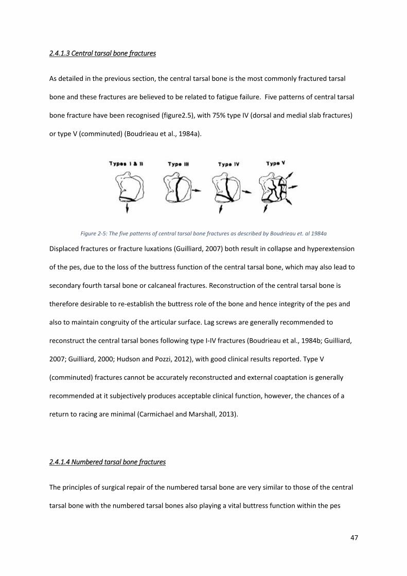
47

2.4.1.3 Central tarsal bone fractures

As detailed in the previous section, the central tarsal bone is the most commonly fractured tarsal

bone and these fractures are believed to be related to fatigue failure. Five patterns of central tarsal

bone fracture have been recognised (figure2.5), with 75% type IV (dorsal and medial slab fractures)

or type V (comminuted) (Boudrieau et al., 1984a).

Figure 2-5: The five patterns of central tarsal bone fractures as described by Boudrieau et. al 1984a

Displaced fractures or fracture luxations (Guilliard, 2007) both result in collapse and hyperextension

of the pes, due to the loss of the buttress function of the central tarsal bone, which may also lead to

secondary fourth tarsal bone or calcaneal fractures. Reconstruction of the central tarsal bone is

therefore desirable to re-establish the buttress role of the bone and hence integrity of the pes and

also to maintain congruity of the articular surface. Lag screws are generally recommended to

reconstruct the central tarsal bones following type I-IV fractures (Boudrieau et al., 1984b; Guilliard,

2007; Guilliard, 2000; Hudson and Pozzi, 2012), with good clinical results reported. Type V

(comminuted) fractures cannot be accurately reconstructed and external coaptation is generally

recommended at it subjectively produces acceptable clinical function, however, the chances of a

return to racing are minimal (Carmichael and Marshall, 2013).

2.4.1.4 Numbered tarsal bone fractures

The principles of surgical repair of the numbered tarsal bone are very similar to those of the central

tarsal bone with the numbered tarsal bones also playing a vital buttress function within the pes

48

(Carmichael and Marshall, 2013). Fractures of these bones are rare (Guilliard, 2010) and generally

involve a dorsal slab fracture which can be reduced and stabilised with lag screws.

2.4.2 Repair following ligamentous injury or degeneration

In contrast to repairs of the talocrural joint, where repair techniques aim to preserve the original

range of motion (Aron and Purinton, 1985b), repair techniques for instability of the more distal

joints; talocalcaneal, proximal intertarsal and tarsometatarsal joints generally involve sacrificing any

motion in favour of promoting a bony arthrodesis.

2.4.2.1 Talocalcaneal luxations.

Gorse et al (1990), reported 5 cases of talocalcaneal luxation secondary to rupture of the

talocalcaneal ligaments. Three of the five cases were treated with a screw positioned from talus to

calcaneus in a lag fashion. One of the two remaining dogs had the luxation stabilised by two figure-of

-eight wires and the final case was treated external coaptation alone. All but one dog, which

developed a post-operative infection had a good clinical outcome. A single case was reported by

Lawson (1960), who used a similar technique but additionally debrided the articular surfaces

between the two bones. In another case series, two of three dogs were treated with a single

talocalcaneal lag screw, and one with coaptation alone producing satisfactory results (Campbell et

al., 1976).

49

2.4.2.2 Proximal intertarsal luxations

Non-surgical management of proximal intertarsal luxations with rest and anti-inflammatories

(Campbell et al., 1976; Dieterich, 1974) or external coaptation (Lawson, 1960) have produced poor

clinical outcomes and are therefore not currently recommended.

Although it appears that most proximal intertarsal luxations affect both the talocentral and

calcaneoquartal joint (Barnes et al., 2013), it has most commonly been recommended to provide

stability across the calcaneoquartal joint alone (Allen et al., 1993; Campbell et al., 1976). Due to the

lack of any biomechanical data to support this recommendation, it is likely that this practice is based

on clinical outcomes from limited numbers of dogs in the previously reported case series.

Although debridement of articular cartilage is a common feature between previous reports, it is

unclear as to what extent that the cartilage must be removed. Whilst it has been recommended to

remove the articular cartilage of both the calcaneoquartal joint and talocentral joint by some

authors (Dieterich, 1974; Lawson, 1960; Whittick, 1975), others have suggested this is unnecessary

(Allen et al., 1993; Campbell et al., 1976).

Following debridement, rigid stabilisation must be provided across the calcaneoquartal joint to

promote arthrodesis. Broadly speaking, stabilisation techniques fall into two categories; bone plate

application and intramedullary techniques that utilise a pin or screw positioned through the

longitudinal axis of the calcaneus and into the fourth tarsal bone. Tension band wires have been

inconsistently applied in reported case series to help resist the bending load endured by the pes.

The earliest report of calcaneoquartal arthrodesis (Lawson, 1960) reports removal of articular

cartilage from the opposing surfaces of the talus, calcaneus, central tarsal bone and fourth tarsal

50

bone with a Volkmann curette. A “reverse nailing” technique was described which involved drilling

from the articular surface of the calcaneus in a proximal direction, before inserting a large screw

from proximal to distal through the calcaneus and into the fourth tarsal bone. A good outcome was

reported in all cases, except one case which died 11 days post operatively. A similar technique was

used by (Campbell et al., 1976) in the majority of their cases, however, a screw length was chosen to

deliberately engage the metatarsal bones distally, although it was noted that on many occasions the

screw passed between these bones. A poorer outcome was seen in dogs who had the

calcaneoquartal joint stabilised with a smooth pin and tension band wire. Screw failure was seen in

two cases; breakage in one case where no attempt was made to remove articular cartilage and

bending of a screw in another. This highlights the large bending forces that implants are subjected

to.

In another large case series, Allen et al. (1993) utilised four techniques, including a single Steinmann

pin alone, a laterally applied 2.7mm bone plate, a Sherman screw and tension band techniques,

which were supported by either a Steinmann pin, Sherman screw, two Kirschner wires. The overall

rate of successful arthrodesis was 85% and no significant difference was observed between all

techniques, however, some groups had only one animal. This finding was in contrast to that of

Campbell et al. (1976), however, like this study, implant failure was also recognised with breakage of

two screws and one Steinmann pin. None of these cases were protected with a tension band wire,

suggesting that a tension band wire may help combat some of the bending forces on the repaired

limb. Loosening of implants were seen in 2 cases and calcaneal fractures reported in a further 2

cases. The clinical results, evaluated by client questionnaires, revealed 81 % of dogs were completely

sound, whilst 19% showed a mild weightbearing lameness.

Subsequent case series commonly utilise bone plate fixation to stabilise the calcaneoquartal joint

and may provide improved stability when compared to the pin and screw techniques, which cannot

provide rotational stability to the same extent as plate fixation. Adequate stability is essential to

51

promote bone formation across the arthrodesis site, which will reduce the risk of cyclic failure of the

implants. (Fettig et al., 2002; Roch et al., 2008; Scrimgeour et al., 2012; Théoret and Moens, 2007) all

report the use of laterally applied bone plates which span across both the calcaneoquartal and

tarsometatarsal joints. Application onto the lateral surface of the pes, results in the plate being

loaded “on edge” as the pes acts as a lever (Devas, 1961). This significantly increases the area

moment of inertia of the implant, reducing the risk of implant deformation.

Whilst (Fettig et al., 2002) recommended a minimum of three screws in the calcaneus and

metatarsals when a hybrid plate was used, none of the other authors provided any recommendation

regarding the configuration of plate stabilisation when attempting to achieve bony union across the

calcaneoquartal joint. Examination of radiographic images from these papers, clearly identifies a lack

of consistency across studies where lateral plates are applied. One case presented by (Fettig et al.,

2002) shows no screws engaging the fourth tarsal bone, whilst another case by the same authors

was performed with a single screw positioned in the fourth tarsal bone that also engaged the central

tarsal bone on the medial aspect of the joint. The radiographic images of (Scrimgeour et al., 2012)

demonstrate another variation, with two screws engaging the fourth tarsal bone. No comparison of

these various configurations is currently available, however, it is likely that changes in plate and

screw configuration may influence the biomechanical performance of the construct as seen in other

scenarios (Field et al., 1999; Törnkvist et al., 1996). The construct configuration is likely influenced by

a number of factors including patient size, plate size and design, underlying pathology and surgeon

preference.

Comparison of clinical outcome following lateral plate repair of calcaneoquartal arthrodesis is

difficult due to the variable outcome measures used by authors. Fettig et al. (2002) reported good

outcomes in 4/4 cases and (Théoret and Moens, 2007) reported good outcomes in 2/2 cases based

on owner assessment, whilst (Roch et al., 2008) evaluated complications, reporting major

complications in only 1/11 cases treated with a lateral plate and this was related to sepsis, with no

52

cases showing implant or bone failure. (Scrimgeour et al., 2012) looked at return to work as a

measure of successful surgery in a series of 14 working dogs with lateral plate repair of either

proximal intertarsal luxation or tarsometatarsal luxation. In this case series, 50% of working dogs

were able to return to full work duties, whilst 4/14 were able to perform most of their duties. The

remaining 3 dogs were unable to return to work following surgery.

Another plating approach described to combat the bending load on the pes, is plantar plating (Wilke

et al., 2000). Here, the plate is located on the biomechanically favourable tension surface of the

bones and the authors report a good outcome in 3 dogs, one dog with objective force plate data that

showed no difference in kinetic parameters between the affected and unaffected limb 7 months

post operatively.

Recently, a large retrospective study (Barnes et al. 2013) was published with the objective to

compare complications and outcomes of calcaneoquartal arthrodesis following one of three

stabilisation techniques; laterally applied bone plate and a figure of eight tension band combined

with either a pin or a screw.

This multicentre study reported 74 procedures, performed in 61 dogs with 58 procedures in the

plate group, nine procedures in the pin group and seven procedures in the screw group. Consistent

with previous reports (Allen et al., 1993; Campbell et al., 1976), implant failure was identified in both

the pin and screw group with breakage, bending and loosening all identified, however, implant

failure was also identified in the plating group, which has not been previously reported in case series

of lateral plate fixation (Fettig et al., 2002; Roch et al., 2008; Théoret and Moens, 2007). In the study

of Barnes et al. (2013), screw loosening was seen in five cases, four involving the fourth tarsal bone

and one involving a screw positioned across multiple metatarsals. Metatarsal fractures (3 cases) and

implant failure (2 cases) were also reported and previous unreported complications. This study

represents the largest collection of cases of calcaneoquartal arthrodesis following non traumatic

disruption of the plantar ligament in dogs to date and concluded that lateral plating was associated

53

with fewer complications compared to screw and pin techniques (Barnes et al., 2013). No attempt

was made to evaluate variables related to the configuration of the implants, such as the number of

plate screws used in each bone or the engagement of metatarsal bones in the pin and screws groups

and therefore no recommendations regarding configuration could be provided.

Dorsal instability at the proximal intertarsal joint is less commonly reported than plantar instability

in dogs (Campbell et al., 1976; Voss et al., 2004)and these two conditions differ biomechanically as

dorsal luxations are likely to be reduced during weight bearing, whilst plantar luxations show

increasing displacement. (Voss et al., 2004) report a case series of 10 dogs and 3 cats treated with

dorsal splinting of the affected joints without debridement of articular cartilage to promote

permanent arthrodesis. Locking plate systems were used in these cases, with good results in 12/13

cases. Joint fusion was identified in 3 cases and two cases suffered from implant breakage, but

without affecting outcome.

2.4.2.3 Tarsometatarsal instability

Instability at the tarsometatarsal joint has been treated in a similar fashion to proximal intertarsal

luxations, with removal of articular cartilage, application of autogenous cancellous bone graft and

stabilisation with internal or external fixation to promote tarsometatarsal arthrodesis.

Campbell et al. (1976) suggested that better outcomes were achieved with lateral plate fixation

compared to compression screwing, wiring and pin-casts, with many of these other techniques

technical challenging to achieve. Good outcomes have been reported in a number of small case

series that were stabilised with lateral plates in a similar fashion to proximal intertarsal luxations.

Dyce et al. (1998) reported a good outcome in 11/11 procedures where a lateral plate was applied to

a subluxated tarsometatarsal joint. Arthrodesis was promoted and achieved in all cases, with 9/11

procedures involving concurrent tarsal or metatarsal fractures. Similar results were reported by Muir

and Norris (1999) who performed plate stabilisation of the tarsometatarsal joint subluxation in 8

dogs, 6 of which has concurrent fractures. No implant breakage was recorded. However, due to the

54

retrospective nature of these studies no attempt was made to standardise plate configuration

making it difficult to provide any recommendations regarding the ideal plate size, screw number and

screw length. As for calcaneoquartal arthrodesis, these is variable engagement of the fourth tarsal

bone, with some cases receiving two screws in the fourth tarsal bone, whilst others received a single

screw. Screw length also varied in these case series with variable engagement of the third or central

tarsal bone on the medial aspect of the pes.

Chow and Balfour (2012) reported a series of 12 dogs and 2 cats that all achieved successful

tarsometatarsal arthrodesis following removal of articular cartilage and stabilisation with 4

intramedullary pins driven from the individual metatarsal bones into the proximal and distal rows of

tarsal bones. The authors suggest, that although the intramedullary pins violated the distal articular

surface of the metatarsals, they provided the benefit of avoiding difficulty in skin closure, as may be

seen with plate repairs. Pin migration and breakage were seen with single pins, however, the

remaining 3 pins in each case remained intact and a successful arthrodesis was achieved.

External skeletal fixation has also been described as a method of fixation to achieve arthrodesis

across the tarsometatarsal joint. Halling et al. (2004) described three cases of tarsometatarsal

stabilisation performed with a circular external skeletal fixator with good results. The mean time

before fixator removal was prolonged (16 weeks), however long term function was good in all cases.

A single case report has described the use of an external skeletal fixator, to provide stabilisation

across the tarsometatarsal joint without debridement of the articular surface, resulting in ankylosis

across these joints. Although good long term clinical function was reported based on owner

assessment, complications were experienced in all 4 cases.

55

56

Section 2.5 Purpose

From this review of the current literature, it is clear that the canine pes plays a vital role in

locomotion and can be damaged through both injury or disease. Despite long recognising that

motion does normally occur within the pes, facilitated by intertarsal bone movement, there is a lack

of understanding regarding the role this motion may play in normal locomotion. Furthermore, no

descriptions of the nature of intertarsal bone motion during weight bearing have been published.

This may reflect the technical challenges posed by attempting to record small magnitudes of motion

in overlapping cuboid bones that are moving at great speed.

Plantar ligament degeneration has been proposed as the underlying cause of proximal intertarsal

subluxation in dogs and despite highly detailed anatomical descriptions of the components of

plantar ligaments, the role these ligaments play in maintaining the integrity of the pes remains

unknown. Furthermore, recommendations for surgical repair to re-establish the integrity of the pes

following injury or disease are based on small, retrospective case series, which report a wide variety

of surgical techniques and implants employed to re-establish force transmission through the canine

pes.

These gaps in our collective knowledge have been the motivation for this thesis, which sets out to

develop new approaches to measure tarsal bone kinematics in the dog, allowing insights into the

cause of clinical conditions, such as proximal intertarsal subluxations, and facilitating evaluation of

surgical procedures, which have been suggested as the most appropriate means of treating such

conditions.

57

Chapter 3 A computed tomography-based

technique for the measurement of canine

tarsal bone kinematics

58

Chapter 3 represents work that has been published as

“Influence of Scan Resolution, Thresholding, and Reconstruction Algorithm on Computed

Tomography-Based Kinematic Measurements” Christopher John Tan, William C. H. Parr, William R.

Walsh, Mariano Makara and Kenneth A. Johnson. J Biomech Eng 139(10), 104503

doi: 10.1115/1.4037558

Abstract from published paper

Radiographic data, including CT and planar x-ray, are increasingly used for kinematic studies in

humans and animals. There is a tendency towards using as high resolution imaging as possible.

Higher resolution imaging is one factor (in conjunction with the reconstruction algorithm) which may

increase the accuracy of reconstructed 3D surface models in representing true bone shape.

However, to date no study has tested the effects of scan resolution, threshold and 3D model

reconstruction algorithm on the accuracy of bone kinematic results. The present study uses a novel

method to do this where canine tarsal bones were positioned on a radiolucent LegoTM board and

scanned before and after undergoing known translations and/or rotations. The DICOM images were

acquired using two different CT scanning resolutions and processed using three different

segmentation threshold levels and three different reconstruction algorithms. Using one bone as the

reference bone, an iterative closest point (ICP) algorithm was used to register bones to a global co-

ordinate system and allow measurement of other bone kinematics in terms of translations and

rotations in and around the x, y, z axes. The measured kinematics were compared to the ‘known’

kinematics, which were obtained from the LegoTM board’s manufacturing standards and tolerances,

to give accuracy error metrics for all bones. The results showed error in accuracy of measured

kinematics was at sub voxel levels (less than 0.5mm). Despite altering the volume and surface area

of the 3D bone models, variation in resolution, segmentation threshold and reconstruction algorithm

had no significant influence upon the accuracy of the calculated tarsal bone kinematics.

59

3.1 Introduction

The field of kinematic analysis of bones has expanded in recent years with the advent of non-

invasive, novel surface matching techniques. Biplanar fluoroscopy techniques, such as X-ray

Reconstruction of Moving Morphology (XROMM) (Brainerd et al., 2010), can be used to calculate in-

vivo kinematics with high degrees of accuracy. However, one limitation of 2D to 3D matching

systems is combatting the challenges posed by complex joints, such as the wrist and ankle, where

there is considerable overlapping of bones (Ito et al., 2015).

For these regions, multiple CT scans have been employed to calculate bone motions between ‘static

states’, for example, at their extreme range of motion (Beimers et al., 2008; Pfaeffle et al., 2005), or

before and after surgical intervention. Similar to biplanar fluoroscopy, non-invasive surface matching

techniques can be employed to identify the positions of the bones in the different CT scans and

hence, record their motion. Surface matching requires generation of 3D models of bones, which can

be generated from the CT data using a number of different techniques and settings.

There is a tendency to acquire CT images at the highest possible resolution (Moore et al., 2015) to

create highly accurate 3D models, which increases exposure to potentially damaging radiation by 30-

50% (Nickoloff and Alderson, 2001).

To date, no study has evaluated the effects of different CT scanning protocols and 3D surface model

reconstruction parameters on the accuracy of the kinematic results obtained from CT data. If

kinematic accuracy is unaffected, then increasing scan resolution (to increase 3D bone

reconstruction precision), with inherent increased radiation exposure, may be unwarranted. The

following experiment aims to test if scan resolution and techniques used for generating 3D bone

models will influence accuracy of kinematic calculations. It was hypothesised that the variations in

scan resolution, threshold levels and reconstruction algorithm will have no significant influence on

the accuracy of calculated kinematics when settings are consistent between scans.

60

3.2. Materials and methods

3.2.1 Specimens

11 canine tarsal bones with soft tissues removed were individually mounted onto plastic building

bricks (Lego® brick, Lego, Billund, Denmark) with double sided padded mounting tape (scotch-

mount, 3M, Pymble, Australia) and polypropylene adhesive film (ConTact, Pomona, CA). The

dimensions of the building bricks were measured using calipers accurate to 0.02mm (Mitutoyo 530-

122, Japan).

All brick-bone constructs were positioned onto a rigid, plastic board (Lego®, Billund, Denmark),

which had two vertical plates attached perpendicularly to the board, and one another (figure 3.1a).

This configuration permitted translation and rotation around and along each (x,y,z) axis. With a

reported manufacturing tolerance of 5 microns (Corbet, 2008), this building block system can

produce accurate and repeatable movements of building blocks.

3.2.2 Image acquisition

A CT scan of the board with 11 brick-bone constructs was performed using a 16 slice helical CT

scanner (Philips Brilliance 16-slice CT scanner). The board was scanned at “high” resolution (120KVP,

117 mA, slice thickness 1mm, slice increment 0.5mm, , 512 X512 matrix, pixel size 0.36mm X

0.36mm ) and again at “low” resolution ( 120KVP, 117 mA, slice thickness 2mm, slice increment

1mm, 512 X512 matrix, pixel size 0.77mm X 0.77mm ). These scans were designated as “before”

scans.

The brick bone constructs were re-arranged on the board (figure 3.1b). The right calcaneus

(reference bone) was not moved. The right fourth tarsal bone (negative control) was removed from

the board, then replaced in its identical location and orientation. The remaining 9 bones underwent

a known translation, rotation or both together as outlined in table 3.1.

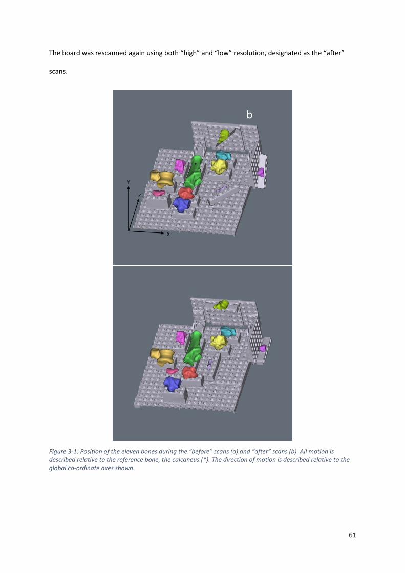
61

The board was rescanned again using both “high” and “low” resolution, designated as the “after”

scans.

Figure 3-1: Position of the eleven bones during the “before” scans (a) and “after” scans (b). All motion is described relative to the reference bone, the calcaneus (*). The direction of motion is described relative to the global co-ordinate axes shown.

a b

b

62

Table 3-1: Known magnitude and direction of the translation or rotation of each bone. CTB = central tarsal bone

Bone Motion Direction (axis) Movement Distance/angle

Right fourth tarsal bone

None

Left CTB Translation X 1 stud across 8.00mm

Left Talus Translation Y 1 plate down 3.20mm

Right third tarsal bone

Translation Z 1 stud across 8.00mm

Right CTB

Translation X 1 stud across 8.00mm

Translation Y 1 plate up 3.20mm

Translation Z 1 stud across 8.00mm

Left fourth tarsal bone

Translation X 1 stud across 8.00mm

Translation Y 1 brick up 9.60mm

Translation Z 2 studs across 16.00mm

Left first tarsal bone

Translation X 2 studs across 16.00mm

Translation Y 1 brick up 9.60mm

Translation Z 1 stud across 8.00mm

Left second tarsal bone

Rotation X 45 degrees

Right first tarsal bone

Rotation Y 45 degrees

Left third tarsal bone

Rotation Z 45 degrees

63

3.2.3 Segmentation and 3D surface model generation

DICOM images were imported to Mimics (version 17.0, Materialize, Belgium) and each bone

segmented using three different Hounsfield unit (HU) threshold levels. Based on a previous pilot

study, segmentation performed with 900HU as the threshold, produced a 3D bone model with a

volume most similar to that of the actual bone, whilst a segmentation threshold of 500HU produced

a 3D bone model with a smaller volume that the original bone a smaller representation.

Segmentation with a 1300HU threshold, produced a 3D bone model with a larger volume than the

original bone. For each threshold level, three 3D surface models were created using pre-defined

marching cubes reconstruction algorithms: “high” accuracy, “optimal” accuracy, “optimal” accuracy

with subsequent smoothing. The “high” accuracy setting applies a matrix reduction and applies 2

iterations of a 0.5 weighted 1st order Laplacian smoothing algorithm and 10 iterations of an

advanced edge mesh reduction algorithm (tolerance = 0.05mm, edge angle = 10o) to the 3D

boundary mesh resulting from the interpolation of the segmented CT slices. The “optimal” accuracy

setting applies no matrix reduction and 2 iterations of a 0.3 weighted 1st order Laplacian smoothing

algorithm and 3 iterations of an advanced edge mesh reduction algorithm (tolerance = 0.0559mm,

edge angle = 10o). The third model was generated using the “optimal” mesh generation setting

followed by application of 2 iterations of a 0.5 weighted 1st order Laplacian smoothing algorithm.

For each 3D surface model, the centre of mass, volume and surface area were recorded.

3.2.4 Initial alignment to a global co-ordinate system

A two-step alignment of ‘before’ and ‘after’ scans was performed prior to kinematic calculations. In

the first step, “before” and “after” scans were manually aligned to the global co-ordinate system in

3-matic 8.0 (Materialize, Belgium) so that the edges of the Lego® board aligned with the X, Y and Z

axes. In this regard, movement of the Lego® bricks between “before” and “after” scan positions

occur along and around the axes of the global co-ordinate system.

64

3.2.5 Calculation of kinematics

For each bone, the movement between the “before” and “after” scan positions was determined 18

times by a single observer: once for every combination of the predictor variables (scan resolution,

threshold level and smoothing protocol). Bone motion was reported in relation to a single reference

bone (right calcaneus).

The second stage of alignment aligned the “after” scans with the “before” scans. This was performed

using the open source program Meshlab (Cignoni et al., 2008). The right calcaneus from the “before”

scan, the Lego board of which was aligned with the global coordinate system in the first step

(described above), was set as the base mesh.

From the “after” scan, the surface meshes of the right calcaneus and the bone of interest were

combined to form a single 3D “shell” of two parts (right calcaneus and the bone of interest).

An Iterative Closest Point (ICP) algorithm (Besl and McKay, 1992)was then used to superimpose the

calcanei of the two scans. This step achieved two important objectives; 1) to align the two scans,

minimising error due to movement of the reference bone between scans and 2) to align the scan to

a meaningful reference coordinate system.

The position of the 3D surface model of the bone of interest from the “before” scan was then

recorded as the “before” position. Again, using a rough manual alignment followed by an ICP

alignment, the 3D surface model of the bone of interest was superimposed on the combined meshes

of the “after” scan. The new position of the 3D surface model of the bone of interest was then saved

as the “after” position. Using this method, the identical 3D surface model was recorded in both the

“before” and “after” position allowing a transformation matrix, consisting of a translation matrix

(mm moved in the global x,y,z coordinate system) and rotation matrix (rotations around the global

coordinate system x, y, z axes) to be calculated (figure 3.2).

65

Figure 3-2: workflow for the scan alignment and calculation of bone kinematics. Initial isosurface reconstructions of the lego boards with bones in the two positions are not aligned with the global coordinate system or one another (A and B). The first step is to align the “before” scan with the global coordinate system (C). The “after” scan is also roughly aligned with the global coordinate system (D). The second stage of alignment uses an ICP algorithm to minimise translational and rotational differences between the scans using the calcaneus (green bone with * shown) of the “before” scan as the fixed entity and superimposing the calcaneus in the “after” scan along to this. The remainder of the “after” lego board and bone models are moved with the “after” calcaneus, but do not influence the alignment (E). The “before” model for each bone is then aligned (again using ICP alignment) with the “after” position and saved separately from the “before” model in the “before” position (F). Thereby, the same 3D model is stored in both “before” and “after” positions.

The translation matrix is calculated by calculating difference between the centroid (mean of all 3D

coordinate points in the mesh) of “before” and “after” 3D surface model positions. The rotation

matrix is calculated in two steps: 1) removing translational differences between the two models by

centering both models at the global coordinate system x, y, z, 0, 0, 0 position and 2) using a Singular

Value Decomposition algorithm (using the the QR algorithm with Given’s rotations (Golub and

Kahan, 1965))implemented in Mathematica (version 10.1, Wolfram, IL, USA) to calculate the

rotation matrix that rotates the 3D surface model from “before” to “after” orientation. The rotation

matrix was then decomposed into the rotations occurring around the global coordinate system x, y,

z axes.

66

The error in kinematic measurement was calculated for each rotation and translation by subtracting

the measured value (acquired from the transformation matrix decomposition) from the known value

(calculated from the building brick dimensions in table 1).

3.2.6 Statistical analysis

All statistical analyses were performed using the commercially available statistical package Genstat

(VSNi, Hemel Hempstead, UK). Descriptive data was performed for the measurement error, including

maximum error, mean, median, and variance. Data were checked for normality using the Anderson-

Darling test before further analysis. For each bone, a general mixed linear model was used to

evaluate the effect of scan resolution (high/low), threshold level (500,900,1300HU), reconstruction

algorithm (high/optimal/additional smoothing) and axis (x/y/z) on the outcome variables. The

measured outcome variables were 3D surface model parameters (co-ordinates of the centre of

mass, model volume and surface area) and the measurement error. Values of p<0.05 were

considered significant. Rotations were known for all bones and included in the calculation of

rotational error. For bones undergoing rotation, a translation would necessarily have occurred. The

translation of the centre of mass of these bones between the “before” and “after” scans was

calculated along the x, y and z axes, however, as the true magnitude of the translation could not be

deduced before the scans, the three bones that underwent rotation were excluded from the

calculation of translational error.

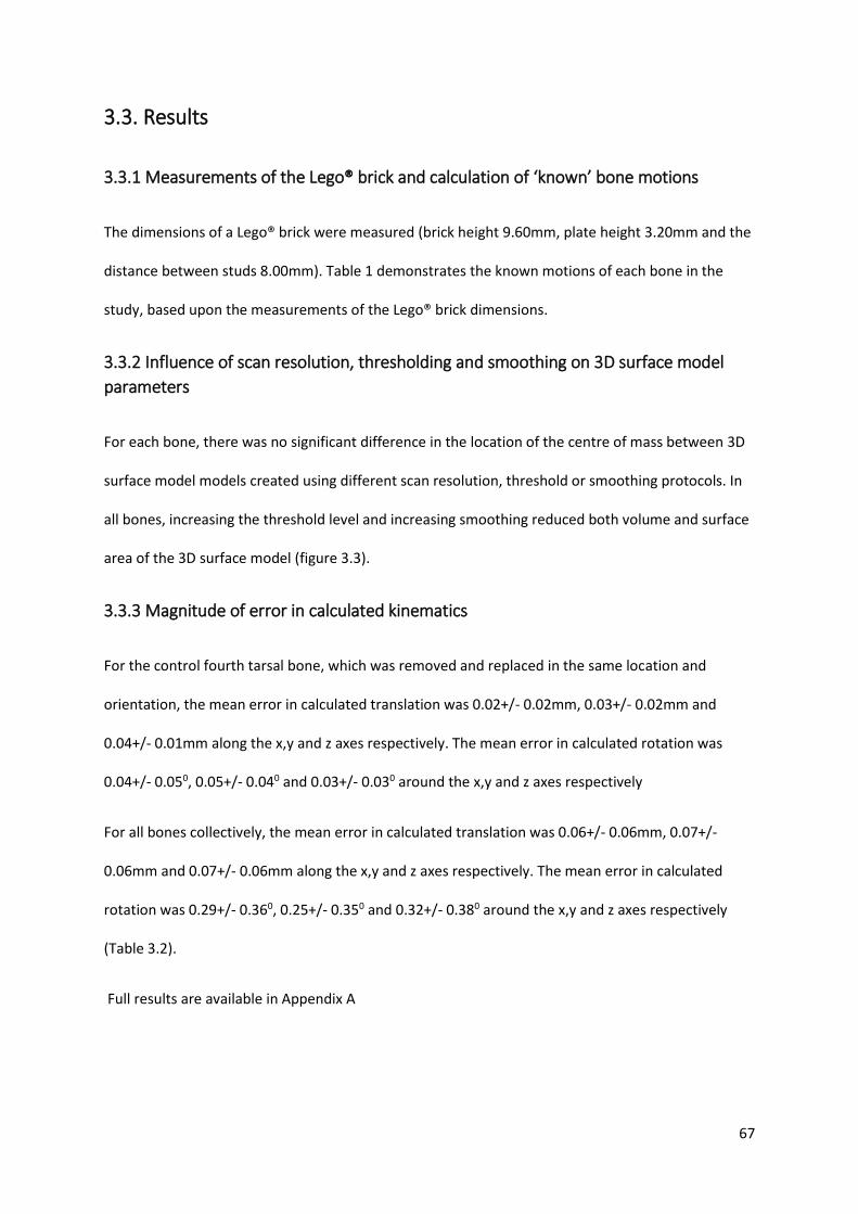
67

3.3. Results

3.3.1 Measurements of the Lego® brick and calculation of ‘known’ bone motions

The dimensions of a Lego® brick were measured (brick height 9.60mm, plate height 3.20mm and the

distance between studs 8.00mm). Table 1 demonstrates the known motions of each bone in the

study, based upon the measurements of the Lego® brick dimensions.

3.3.2 Influence of scan resolution, thresholding and smoothing on 3D surface model

parameters

For each bone, there was no significant difference in the location of the centre of mass between 3D

surface model models created using different scan resolution, threshold or smoothing protocols. In

all bones, increasing the threshold level and increasing smoothing reduced both volume and surface

area of the 3D surface model (figure 3.3).

3.3.3 Magnitude of error in calculated kinematics

For the control fourth tarsal bone, which was removed and replaced in the same location and

orientation, the mean error in calculated translation was 0.02+/- 0.02mm, 0.03+/- 0.02mm and

0.04+/- 0.01mm along the x,y and z axes respectively. The mean error in calculated rotation was

0.04+/- 0.050, 0.05+/- 0.040 and 0.03+/- 0.030 around the x,y and z axes respectively

For all bones collectively, the mean error in calculated translation was 0.06+/- 0.06mm, 0.07+/-

0.06mm and 0.07+/- 0.06mm along the x,y and z axes respectively. The mean error in calculated

rotation was 0.29+/- 0.360, 0.25+/- 0.350 and 0.32+/- 0.380 around the x,y and z axes respectively

(Table 3.2).

Full results are available in Appendix A

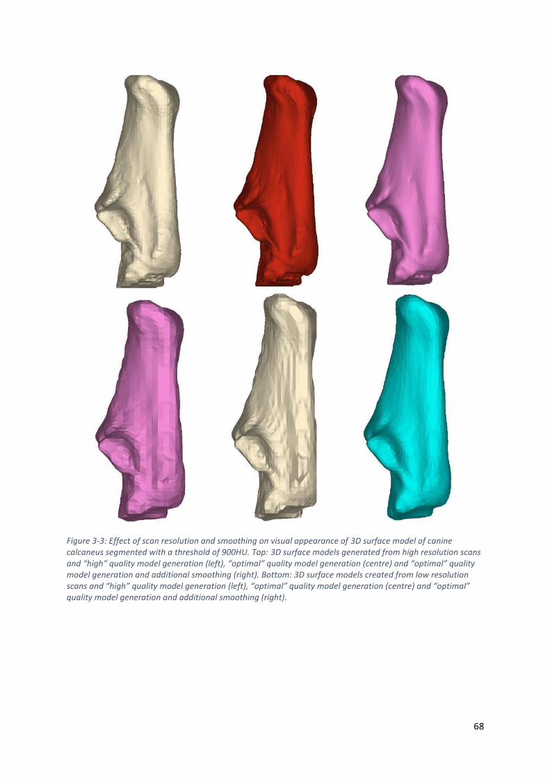
68

Figure 3-3: Effect of scan resolution and smoothing on visual appearance of 3D surface model of canine calcaneus segmented with a threshold of 900HU. Top: 3D surface models generated from high resolution scans and “high” quality model generation (left), “optimal” quality model generation (centre) and “optimal” quality model generation and additional smoothing (right). Bottom: 3D surface models created from low resolution scans and “high” quality model generation (left), “optimal” quality model generation (centre) and “optimal” quality model generation and additional smoothing (right).

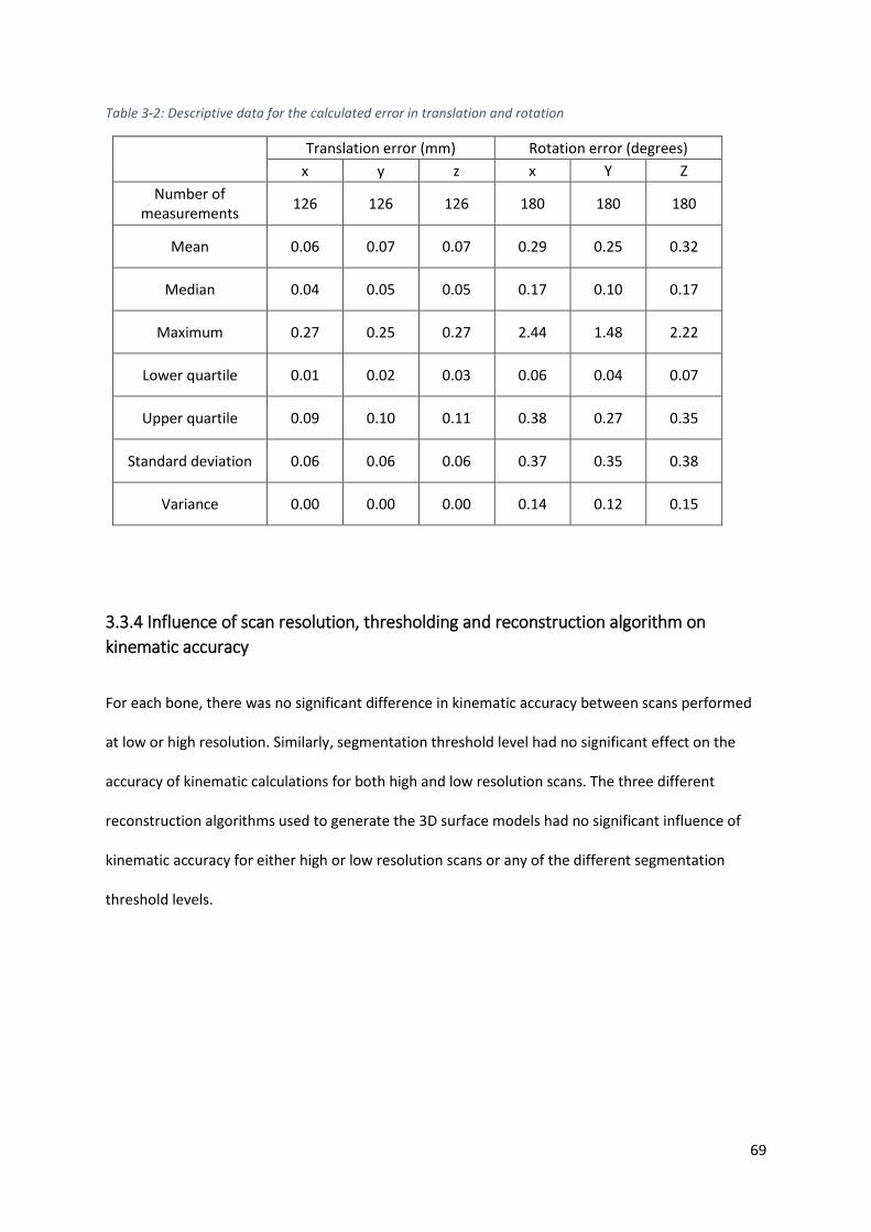
69

Table 3-2: Descriptive data for the calculated error in translation and rotation

Translation error (mm) Rotation error (degrees) x y z x Y Z

Number of measurements

126 126 126 180 180 180

Mean 0.06 0.07 0.07 0.29 0.25 0.32

Median 0.04 0.05 0.05 0.17 0.10 0.17

Maximum 0.27 0.25 0.27 2.44 1.48 2.22

Lower quartile 0.01 0.02 0.03 0.06 0.04 0.07

Upper quartile 0.09 0.10 0.11 0.38 0.27 0.35

Standard deviation 0.06 0.06 0.06 0.37 0.35 0.38

Variance 0.00 0.00 0.00 0.14 0.12 0.15

3.3.4 Influence of scan resolution, thresholding and reconstruction algorithm on

kinematic accuracy

For each bone, there was no significant difference in kinematic accuracy between scans performed

at low or high resolution. Similarly, segmentation threshold level had no significant effect on the

accuracy of kinematic calculations for both high and low resolution scans. The three different

reconstruction algorithms used to generate the 3D surface models had no significant influence of

kinematic accuracy for either high or low resolution scans or any of the different segmentation

threshold levels.

70

3.4 Discussion

The ICP (surface morphology based) registration method used in this study showed a high level of

accuracy when measuring bone motion using a variety of canine tarsal bones. The results are

comparable to previous studies (Crisco et al., 1999; Pfaeffle et al., 2005) although quantitative

comparisons of results is difficult due to variations in the methods used and metrics reported.

Accurate detection of small motions may be vitally important in the diagnosis of conditions such as

joint instability and in the evaluation of post-operative range of motion, particularly in multiple level

joints, such as the carpus and tarsus, where palpation and radiographs alone may be inadequate.

Higher scan resolutions, with reduced voxel size, may make subsequent bone segmentation simpler,

but will increase the radiation exposure. Patel et al. demonstrated a nominal increase in error with

increased pitch using tissue-based classification registration (Marai et al., 2006). The experiment

performed in this chapter, using a 16-slice CT scanner and surface-based registration method,

demonstrated no decrease in kinematic accuracy with lower resolution scanning, suggesting that a

reduction in radiation exposure may be possible when measuring kinematics alone. However, when

investigating kinematics in a conscious patient, the scan acquisition time (determined by number of

slices the CT machine may obtain per revolution) may also play a significant role in kinematic

accuracy as motion artefact may impact kinematic accuracy.

Formation of the 3D bone models from the multiple DICOM images produced from the CT scan

involves segmentation of the bone of interest and generation of a surface, which is subsequently

used for kinematic calculation. Segmentation can be performed by manual pixel selection but

generally semi-automated segmentation is utilized to increase the efficiency of the process. Altering

threshold segmentation levels had a significant influence on surface area and volume; however, it

had no effect on the accuracy of measured rotations and translations, presumably as the effect of

thresholding level is uniform across the entire surface of the bone (figure 3.4). When kinematics

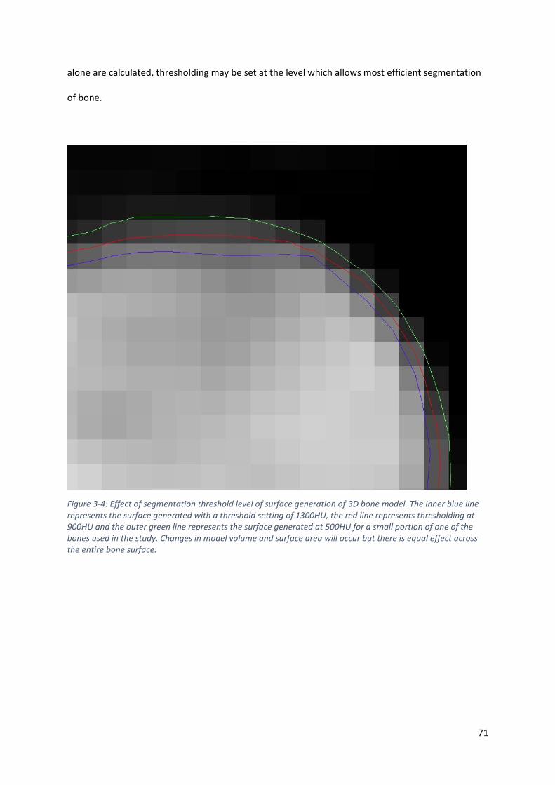
71

alone are calculated, thresholding may be set at the level which allows most efficient segmentation

of bone.

Figure 3-4: Effect of segmentation threshold level of surface generation of 3D bone model. The inner blue line represents the surface generated with a threshold setting of 1300HU, the red line represents thresholding at 900HU and the outer green line represents the surface generated at 500HU for a small portion of one of the bones used in the study. Changes in model volume and surface area will occur but there is equal effect across the entire bone surface.

72

Reconstruction algorithms that included additional smoothing reduced both surface area and

volume of the bones in this study. The reconstruction algorithms with smoothing produce bone

models that more closely resemble the actual bone specimen (figure 3.3); however, smoothing had

no significant impact upon calculated bone motions. This finding suggests that reconstruction

algorithms with additional smoothing following segmentation may be applied to produce more

accurate visual representations, but is unnecessary in kinematic calculations. The elimination of

smoothing from any protocol may produce a more time efficient method of kinematic calculation.

One limitation of this study is the use of bone specimens that are no longer in close proximity to

each other and covered with soft tissues. Segmentation may have been more accurate and

repeatable compared to in vivo studies, in which segmentation may prove challenging. However, it

would be extremely difficult to perform accurate known bone motions, which are used as a “gold

standard”, in an ex vivo situation. It must also be recognized that these findings may only apply to

this particular surface based method of kinematic measurement and must be validated against other

methods, such as inertia based techniques. This study utilized canine tarsal bones, which display a

generally globular geometry. Although it has been shown that obtaining accurate CT based

kinematic data in globular bones is more challenging than elongated bones (Crisco et al., 1999), care

must be taken when extrapolating these results to bones of different geometry. The techniques

described here may also permit kinematic calculations on other tissues such as ocular and vascular

tissues, however, further studies optimized for visualizing these particular tissues would be required

to validate this technique. A lack of contrast between soft tissues may influence accuracy and any

conclusion regarding soft tissue kinematics is beyond the scope of this present study.

These is also the potential for error introduced when the CT scans were aligned to our co-ordinate

system. This alignment was performed visually and this step was introduced so motion could be

described along the axes of the LEGO board and to reduce errors associated with inaccurate

placement of the LEGO board on the CT gantry. Another source of inaccuracy may have originated

73

from variation in measurement between trials. Although not performed as part of this study,

multiple measurement trials would help identify the magnitude of variability from variation in

measurement between trials.

Although no significant difference was identified in regard to scan resolution, a power calculation

was not performed and hence it is possible that the failure to identify any significant difference

could be related to a type II error.

74

3.5 Conclusions

The findings of this study show that scan resolution, segmentation threshold level and the

reconstruction algorithm used to generate 3D surface models have no significant (p = 0.05) influence

on the magnitude of error in tarsal bone kinematics (rotations and translations). Lower resolution

scanning is therefore recommended to reduce radiation exposure without compromising kinematic

accuracy.

75

Chapter 4 Development of an ex vivo limb

loading device

76

4.1 Chapter Introduction

Kinematic studies reveal the unique patterns of movement across different joints and improve our

understanding of both normal and diseased conditions. A huge variety of measurement techniques

and experimental designs have been reported. These techniques may be categorised based upon

their level of tissue disruption. Whilst non-invasive techniques preserve the surrounding tissues,

their usefulness may be limited by a lack of coupling between external marker motion and the

motion of the underlying bone (Benoit et al., 2006; Kim et al., 2011). Additionally, variation in

marker positioning can also influence kinematic measurements (Torres et al., 2011).

Imaging based techniques are non-invasive and directly measure bone motion, however, the subject

must remain in the imaging field, which generally surrounds the patient.

Invasive techniques, such as the use of cortical pins, allow 3D tracking of bones in real time, but

require a surgical procedure, which may alter the kinematic patterns through disruption of soft

tissue structures (Lundgren et al., 2008). Additionally, the smaller tarsal bones, such as the

cuneiforms (in humans) and numbered tarsal bones (in dogs) are difficult to instrument with invasive

markers. Despite the relative larger size of the human tarsal bones, many are considered too small

to instrument with pins (Wolf et al., 2008). Failure to measure motion of each bone will introduce

kinematic errors due to violations of rigid body assumptions (Nester et al., 2010).

Kinematic studies can also be classified as dynamic, where continuous data is collected in real time,

or static, where bone position may be recorded at certain points in time. Depending on the variable

being measured, static studies have been shown to be as accurate as dynamic studies (Foumani et

al., 2009).

Kinematic experiments can be performed in vivo or ex vivo using cadaveric specimens, each with

their own limitations. The kinematics recorded in vivo are the result of both external forces (if

applied) and internal forces (muscular contractions) and are considered the most representative of

77

true bone motions. Reproducing the muscular forces during cadaveric experiments is important as

this has been shown to alter kinematic patterns (Foumani et al., 2010; Hamel et al., 2004; Sharkey

and Hamel, 1998). The advantages of cadaveric specimens include the ability to perform additional

procedures and correlate kinematic results with dissection of specimens.

In veterinary medicine, cadaveric limb loading jigs that replicate the major muscular forces acting on

the stifle joint have greatly improved our understanding of stifle biomechanics and surgical

interventions. The ideal limb loading jig should consistently reproduce the intended force on the

limb, be re-usable and applicable to limbs of differing size and potentially even different species.

To allow for the further investigation of kinematics of the canine tarsal joint, a limb loading jig was

designed to replicate both the internal and external forces exerted on the canine tarsal joint.

Utilising the CT based kinematic measurement techniques described in the previous chapter, this jig

could then be used to improve our understanding of normal motion and the pathophysiology of

disease in the canine tarsal joint.

In this chapter, four sequential experiments detailing the development and the validation of the limb

loading jig are reported.

78

4.2 Experiment 1: Initial concepts and jig design: phase 1

4.2.1 Introduction

Limb loading jigs have been developed to replicate muscular forces across the stifle of both dogs

(Apelt et al., 2007; Hoffmann et al., 2011; Warzee et al., 2001)and cats (Kneifel et al., 2017). These

limb presses apply a load to the femur and collapse of the specimen (by flexion of the stifle and

hock) is counteracted by replication of the forces generated by the stifle extensors (quadriceps

muscle) and hock extensors (gastrocnemius muscle).

In these limb presses, the quadriceps muscle is replaced with a spring that connects the patella and

proximal femur, whilst a cable with turnbuckle connects the caudodistal femur to the tuber calcanei.

The turnbuckle allows alteration to the length of the cable, which simulates the forces of the

gastrocnemius muscle and hence allows alteration to the joint angles (Warzee et al., 2001).

One potential concern when replacing the natural insertion of the muscle with a bone tunnel or bone

screw, is the alteration of the tensile force of the tendon. Altering the direction of pull may influence

the motion of the bone and therefore alter kinematic measurements. To best replicate the force of a

muscle on bone, some jig designs incorporate small motors that can be attached to the tendon of

muscle and preserve the complex enthesis (Hamel et al., 2004; Sharkey and Hamel, 1998).

When investigating kinematics of the canine tarsal joint in cadaveric specimens during the stance

phase, the effect of the tarsal extensors must be replicated. The tarsal joint is extended when a tensile

force is exerted through the attachment of the common calcaneal tendon on the tuber calcanei. This

tendon comprises the tendon of insertion of the gastrocnemius muscle, superficial digital flexor and

the conjoined tendon of semitendinosus, gracillis and biceps femoris muscles (Evans et al., 2012).

79

As the gastrocnemius muscle contracts eccentrially during weight bearing and undergoes minimal

change in length (Goslow et al., 1981), the aim of this experiment was to evaluate if the intact

gastrocnemius muscle would maintain hock extension during axial loading of the tibia.

It was hypothesised that immobilisation of the stifle joint and preservation the gastrocnemius

muscle would maintain tarsal extension during application of load to the tibia.

80

4.2.2 Materials and methods

A limb loading jig was constructed and comprised a proximal limb holding constraint, a base plate

upon which the foot was positioned and a compression mechanism to simulate load bearing.

4.2.2.1 Limb preparation

All limbs were obtained from adult greyhounds euthanased for reasons unrelated to this study.

Limbs were prepared by transection of the femur proximal to the insertion of the gastrocnemius

muscle. Care was taken to preserve the insertion of the gastrocnemius and superficial digital flexor

muscle. All other muscles proximal to the stifle were removed. Limbs were wrapped in saline soaked

cloth and frozen at -20 degrees until use. Limbs were thawed at 4 degrees overnight prior to use.

A Steinmann pin (4.8 mm diameter) was positioned transarticularly across the stifle joint. With the

stifle fully flexed, the pin was first driven proximally from the intercondylar notch to exit through the

cranial cortex of the femur proximal to the trochlea. The stifle was then extended to approximately

135 degrees to simulate the mean stifle angle measured during the stance phase of a walk

(Hottinger et al., 1996). The pin was then driven distally to engage the tibial condyle and cranial tibial

cortex (figure 4.1).

81

Figure 4-1: Method of stifle immobilisation. The stifle was immobilised by a 4.8mm diameter Steinmann pin positioned transarticularly. The stifle was extended to approximately 135 degrees to simulate the stifle angle during the mid-stance phase of the walk. The medial collateral ligament (arrow) was used as a landmark to produce a consistent starting point for the second trans-tibial pin.

82

A second 4.8mm diameter pin, termed the trans-tibial pin, was driven through the proximal tibial

metaphysis in a medial to lateral direction. The starting position of this pin was located

approximately 5mm below (distal) to the proximal articular surface of the tibia and through the

middle of the medial collateral ligament (figure 4.1). Insertion of a 25Ga needle through the medial

collateral ligament facilitated accurate identification of this position.

The trans-tibial pin was used to apply a simulated weight bearing load to the limb using the loading

mechanism of the jig.

4.2.2.2 Proximal restraint

To constrain the trans-tibial pin during loading, approximately one quarter the circumference of a

100mm diameter PVC pipe was removed longitudinally. Two longitudinal slots were then cut in the

pipe to accommodate the trans-tibial pin (figure 4.2). The pipe was attached directly to the foot

plate by a single wood screw.

4.2.2.3 Foot plate

The foot plate was constructed with a series of structural pine blocks attached to the PVC piping.

4.2.2.4 Loading mechanism

Two “tie down” straps were hooked over each end of the trans-tibial pin. To prevent slippage of the

hooks off the ends of the pin, two external skeletal fixator clamps were placed on either end of the

pin. The tie down straps were then connected behind the base plate by interlinking their hooks. The

tie down straps use a ratchet mechanism to shorten and then maintain their length. The limb was

compressed as the ratchets of the tie down straps were alternatively tightened (figure 4.2).

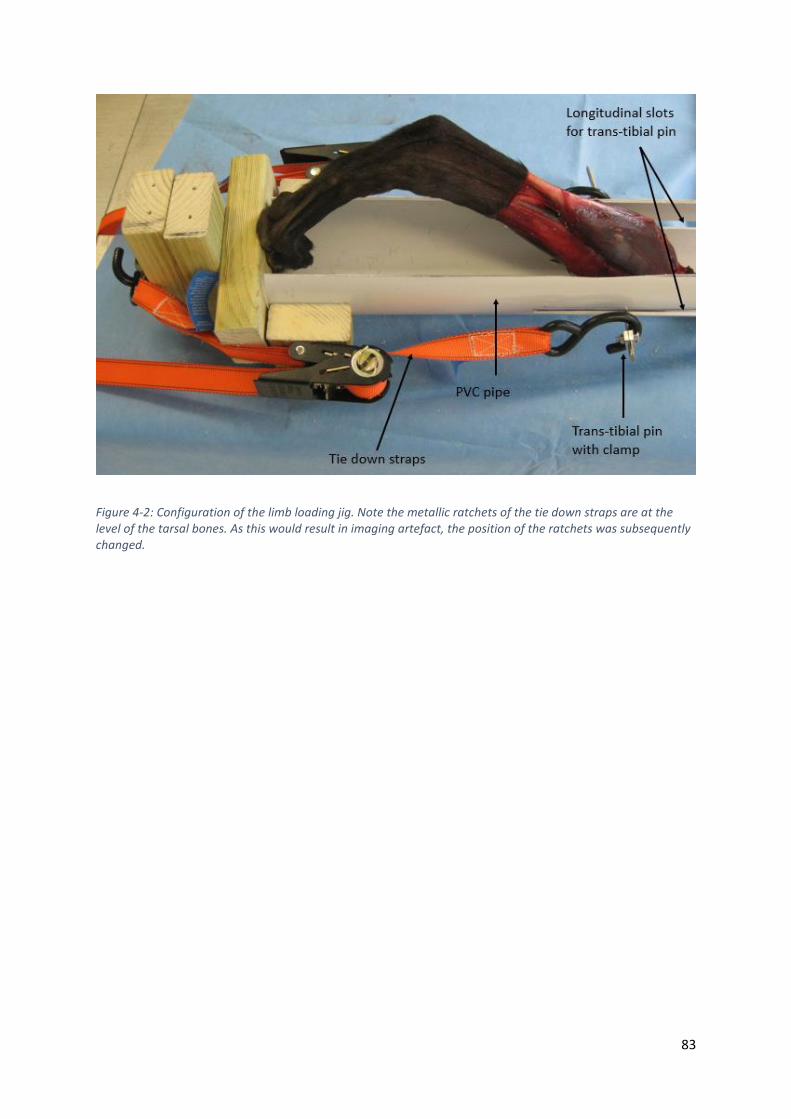
83

Figure 4-2: Configuration of the limb loading jig. Note the metallic ratchets of the tie down straps are at the level of the tarsal bones. As this would result in imaging artefact, the position of the ratchets was subsequently changed.

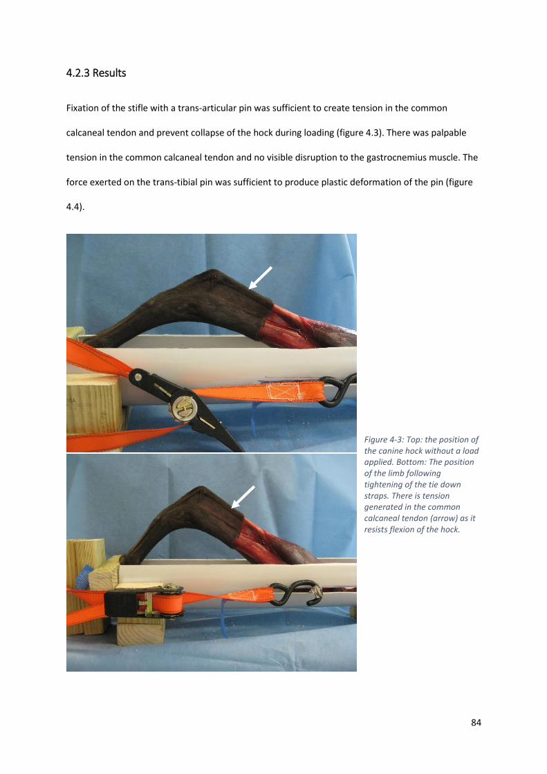
84

4.2.3 Results

Fixation of the stifle with a trans-articular pin was sufficient to create tension in the common

calcaneal tendon and prevent collapse of the hock during loading (figure 4.3). There was palpable

tension in the common calcaneal tendon and no visible disruption to the gastrocnemius muscle. The

force exerted on the trans-tibial pin was sufficient to produce plastic deformation of the pin (figure

4.4).

Figure 4-3: Top: the position of the canine hock without a load applied. Bottom: The position of the limb following tightening of the tie down straps. There is tension generated in the common calcaneal tendon (arrow) as it resists flexion of the hock.

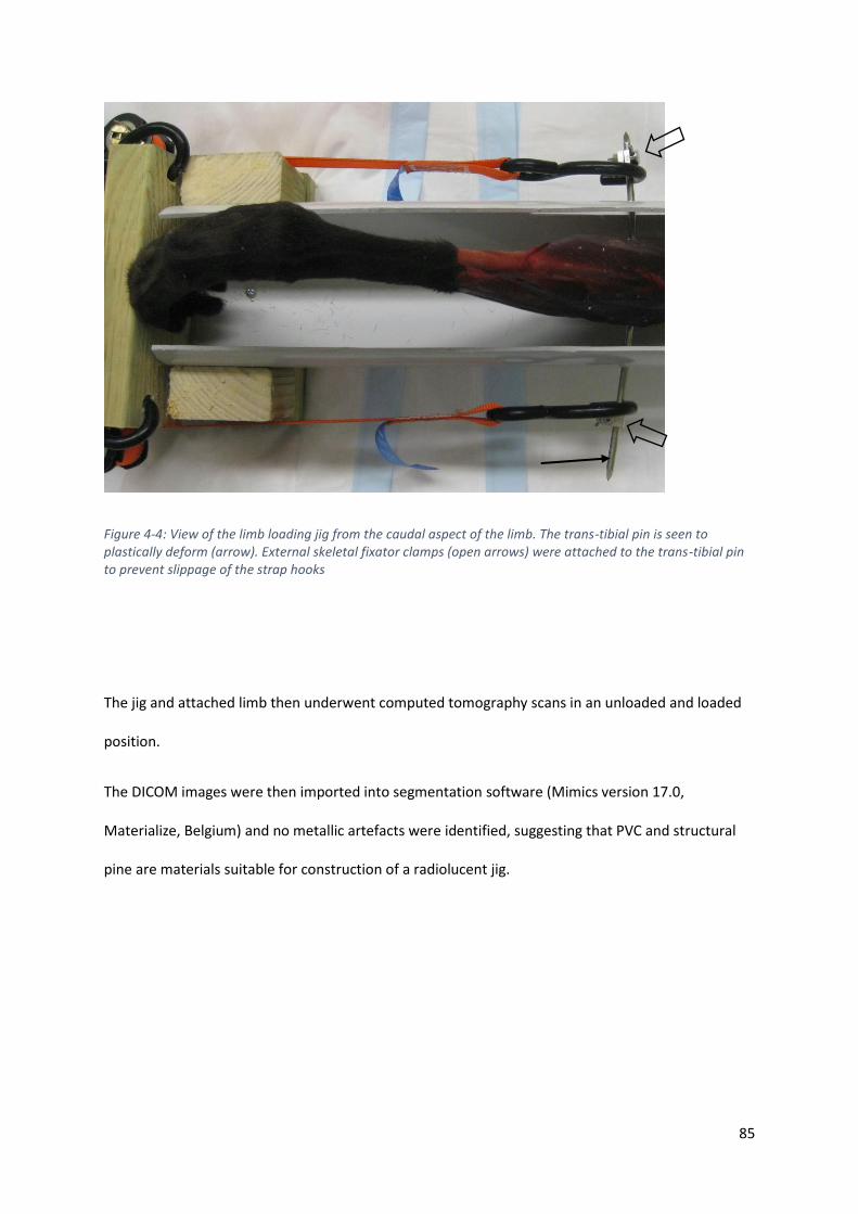
85

Figure 4-4: View of the limb loading jig from the caudal aspect of the limb. The trans-tibial pin is seen to plastically deform (arrow). External skeletal fixator clamps (open arrows) were attached to the trans-tibial pin to prevent slippage of the strap hooks

The jig and attached limb then underwent computed tomography scans in an unloaded and loaded

position.

The DICOM images were then imported into segmentation software (Mimics version 17.0,

Materialize, Belgium) and no metallic artefacts were identified, suggesting that PVC and structural

pine are materials suitable for construction of a radiolucent jig.

86

4.2.4 Discussion

The results of this experiment, demonstrate that immobilisation of the stifle joint and preservation

of the gastrocnemius muscle and common calcaneal tendon was sufficient to passively restrict hock

flexion when a compressive load was applied to the tibia, supporting the original hypothesis.

This finding is likely to reflect the strong connective tissue that surrounds the gastrocnemius muscle

and also contributes to a significant internal framework that infiltrates around the pennate

arrangement of the muscular fibres. The cadaveric gastrocnemius musculotendinous unit was able

to resist high loads during passive stretching, although the tension was not measured in this pilot

experiment.

During limb compression, bending forces were generated if the foot pads were not positioned

directly in the line between the trans-tibial pin and the point where the tiedown straps were joined

under the base plate. These bending forces resulted in separation of the PVC pipe and wooden base

plate. This precarious balance was also noted in previous limb press devices (Hoffmann et al., 2011),

which were subsequently modified by the addition of a caudal tensioner that allowed a wider range

of joint angles to be studied. The delicate balance in this situation could be overcome with a more

rigid frame to connect the base plate and proximal restraint. The addition of a restraint as suggested

by others (Hoffmann et al., 2011) may alter the physiological loading pattern of the limb and was not

considered as a solution for future jigs due to original aim of ensuring accurate representation of

internal and external forces on the cadaveric limb.

The ratchet mechanism was also located at the level of the tarsal bones which would have created

artefact if left unchanged (figure 4.3). The position of the ratchets was subsequently moved distal to

the foot plate leaving only the tape webbing crossing the bones of interest (figure 4.4). Future jigs

may overcome this problem by changing the loading mechanism from a tension generating

mechanism, which naturally must span from foot plate to proximal restraint, to a compression

87

generating device This device could be positioned behind either the foot plate or proximal restrain,

thereby avoiding the mechanism producing unwanted imaging artefact.

The trans-tibial pin was observed to plastically deform at higher loads (figure 4.4), which may reduce

the ability to apply a clinically relevant load to the limb. The greater the distance between the tibia

and the point where a force is applied, the greater the bending moment generated (Johnson and

DeCamp, 1999). Future jigs would benefit from reducing the working length of the trans-tibial pin by

applying the force as close to the tibia as possible. Other alternatives to prevent bending of the

trans-tibial pin include increasing the pin dimeter, which will increase the area moment of inertia, a

geometric measure which dictates a structure’s ability to resist a bending load. Selecting a different

material for use as the trans-tibial pin could potentially increase bending resistance. Amongst the

commonly used materials for orthopaedic implants, 316L stainless steel has a high modulus of

elasticity, about twice that of titanium alloys, with only cobalt chrome alloys having a higher

modulus (Niinomi, 2002). Selecting highly cold worked metals will also increase resistance to

bending. In contrast to orthopaedic wire, which is minimally cold worked and bone plates, which are

moderately cold worked, intra-medullary nails are highly cold worked and therefore most resistant

to bending (Johnson et al., 2005).

88

4.3 Experiment 2: Jig design phase 2

4.3.1 Introduction

The direction and magnitude of any bone movement is the result of tensile forces acting at

tendinous insertions during muscular contraction, force from the adjacent bones and a restriction in

movement from connective tissues such as ligaments and the joint capsule.

When cadaver based kinematic studies are performed, the force from adjacent bones and restriction

in motion due to ligaments and the joint capsule are more readily reproduced. Re-creating muscular

forces is more challenging. In our previous experiment, the stifle joint was immobilised and this was

adequate to maintain tension in the intact gastrocnemius muscle and superficial digital flexor

muscles, resisting hock flexion during loading of the tibia.

Preservation of the enthesis of the tuber calcanei allows replication of the natural complex tensile

force on this bone, which is a major determinant of the kinematics of the calcaneus and

neighbouring tarsal bones. The calcaneus exerts both a tensile force on adjacent bones (via strong

ligamentous connections) and a compressive force (through compression of adjacent articular

cartilage). This reproduction of internal forces within the tarsus is an important aspect of kinematic

calculations in cadaveric specimens.

The aim of this experiment was to redesign the limb loading jig in order to address the problems

associated with the previous jig, such as the balance of the limb and deformation of the apparatus.

An additional aim was to create a jig that could replicate a range of external forces that best

simulate a dog performing normal activity at high speeds. In galloping dogs, a ground reaction force

of approximately 1.6 times body weight has been recorded (Walter and Carrier, 2007), which

equates to approximately 560N in a 35kg dog

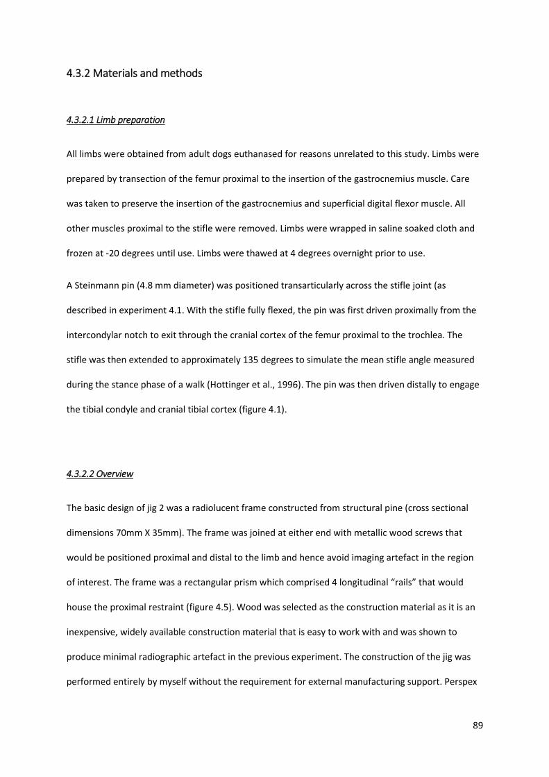
89

4.3.2 Materials and methods

4.3.2.1 Limb preparation

All limbs were obtained from adult dogs euthanased for reasons unrelated to this study. Limbs were

prepared by transection of the femur proximal to the insertion of the gastrocnemius muscle. Care

was taken to preserve the insertion of the gastrocnemius and superficial digital flexor muscle. All

other muscles proximal to the stifle were removed. Limbs were wrapped in saline soaked cloth and

frozen at -20 degrees until use. Limbs were thawed at 4 degrees overnight prior to use.

A Steinmann pin (4.8 mm diameter) was positioned transarticularly across the stifle joint (as

described in experiment 4.1. With the stifle fully flexed, the pin was first driven proximally from the

intercondylar notch to exit through the cranial cortex of the femur proximal to the trochlea. The

stifle was then extended to approximately 135 degrees to simulate the mean stifle angle measured

during the stance phase of a walk (Hottinger et al., 1996). The pin was then driven distally to engage

the tibial condyle and cranial tibial cortex (figure 4.1).

4.3.2.2 Overview

The basic design of jig 2 was a radiolucent frame constructed from structural pine (cross sectional

dimensions 70mm X 35mm). The frame was joined at either end with metallic wood screws that

would be positioned proximal and distal to the limb and hence avoid imaging artefact in the region

of interest. The frame was a rectangular prism which comprised 4 longitudinal “rails” that would

house the proximal restraint (figure 4.5). Wood was selected as the construction material as it is an

inexpensive, widely available construction material that is easy to work with and was shown to

produce minimal radiographic artefact in the previous experiment. The construction of the jig was

performed entirely by myself without the requirement for external manufacturing support. Perspex

90

was also considered as a manufacturing material but was considerably more expensive and more

brittle, making it harder to work with.

Figure 4-5: The redesigned jig (jig2) with a frame that comprised 4 beams of structural pine and housed the proximal limb restraint and foot plate (not shown above). Wood was selected as the construction material as it was inexpensive, radiolucent and easy to work with. The open sides allow the operator to visualise the limb position from two orthogonal positions.

4.3.2.3 Proximal restraint

The proximal limb restraint originally comprised two L-shaped aluminium brackets that would secure

the limb to a wooden disc positioned within the 4 “rails” of the frame (figure 4.6). The brackets were

positioned centrally on the disc. Initial testing showed that brackets placed on a single disc were

inadequate to prevent angulation of the limb (a problem in the previous experiment). This “delicate

balance” has been identified in previous limb presses (Hoffmann et al., 2011). The addition of a

second disc created a cylindrical shape to the proximal restraint (figures 4.5 and 4.7) thereby

constraining the proximal device so only axial motion and rotation were permitted.

A 5mm bone tunnel was drilled from medial to lateral through the proximal tibial metaphysis. The

tunnel was positioned approximately 5mm distal to the articular surface, which was identified with

insertion of a series of 25Ga needles. The craniocaudal position of the tunnel was approximately half

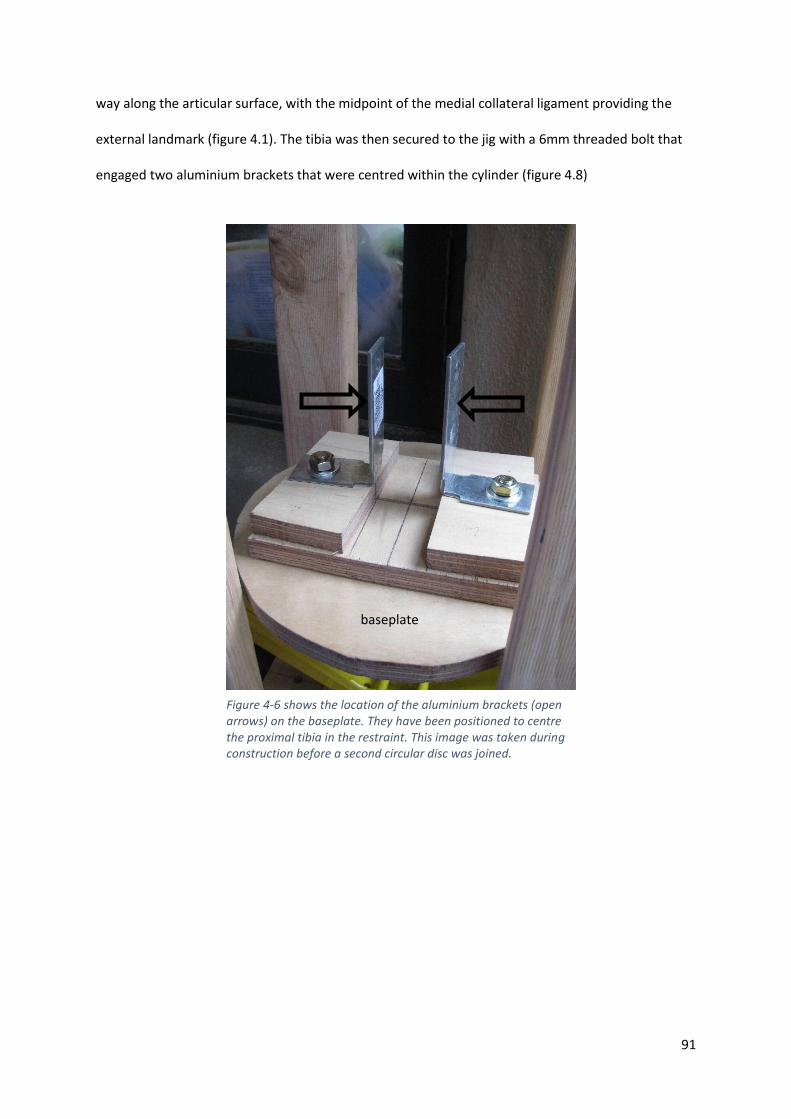
91

way along the articular surface, with the midpoint of the medial collateral ligament providing the

external landmark (figure 4.1). The tibia was then secured to the jig with a 6mm threaded bolt that

engaged two aluminium brackets that were centred within the cylinder (figure 4.8)

baseplate

Figure 4-6 shows the location of the aluminium brackets (open arrows) on the baseplate. They have been positioned to centre the proximal tibia in the restraint. This image was taken during construction before a second circular disc was joined.

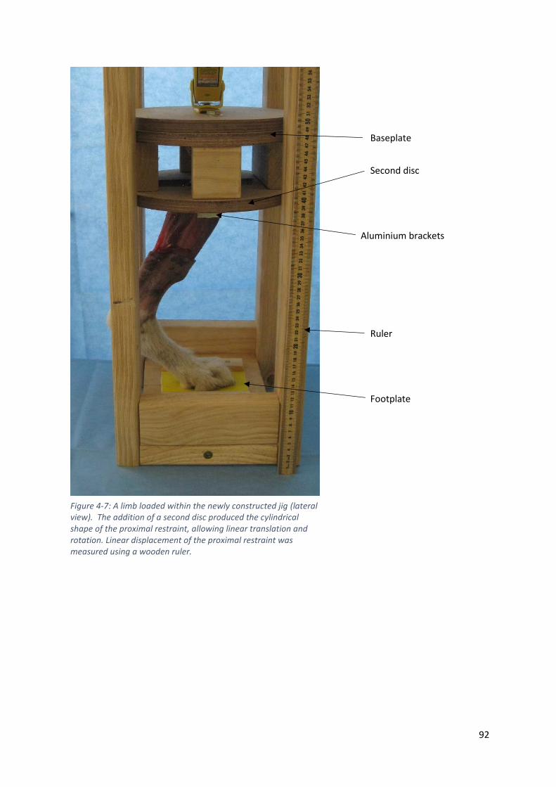
92

Baseplate

Second disc

Aluminium brackets

Ruler

Footplate

Figure 4-7: A limb loaded within the newly constructed jig (lateral view). The addition of a second disc produced the cylindrical shape of the proximal restraint, allowing linear translation and rotation. Linear displacement of the proximal restraint was measured using a wooden ruler.

93

Figure 4-8: Cranial view of the jig with limb loaded. The proximal tibia is secured to the jig with a 6mm threaded bolt positioned through a previously drilled bone tunnel (yellow arrow). The distance between the aluminium brackets was customised to decrease the distance between bracket and the limb. This would reduce bending forces on the trans-tibial pin.

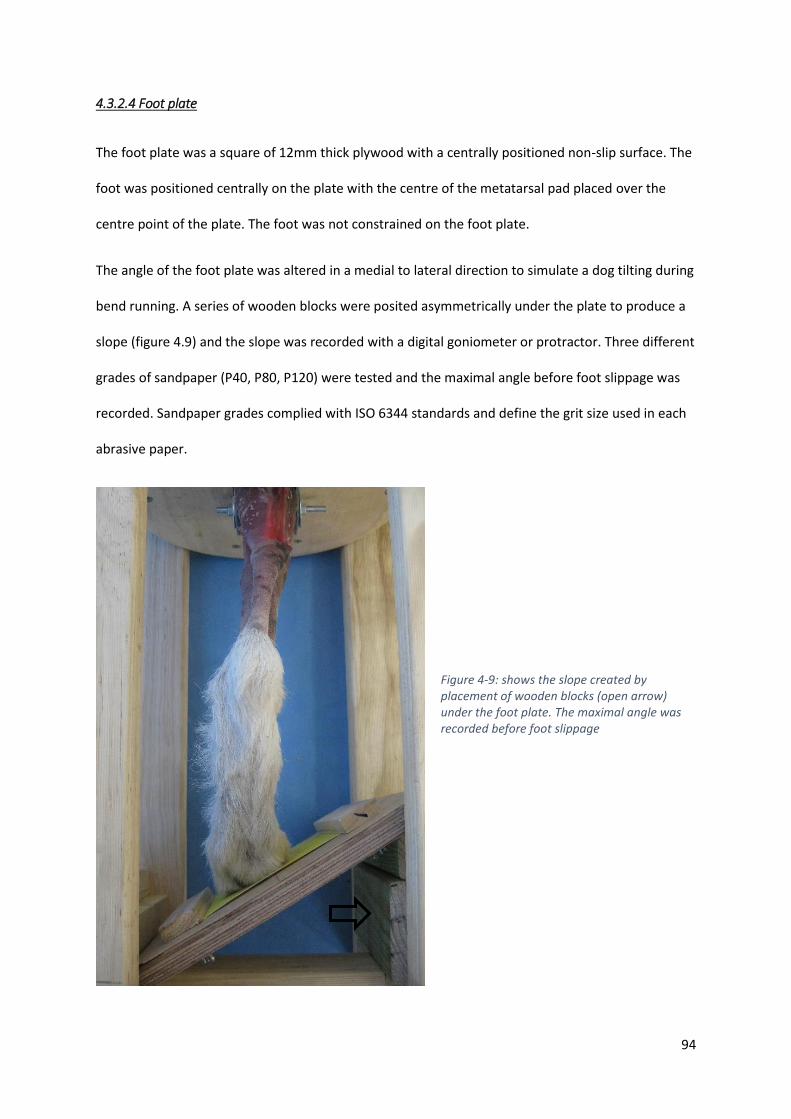
94

4.3.2.4 Foot plate

The foot plate was a square of 12mm thick plywood with a centrally positioned non-slip surface. The

foot was positioned centrally on the plate with the centre of the metatarsal pad placed over the

centre point of the plate. The foot was not constrained on the foot plate.

The angle of the foot plate was altered in a medial to lateral direction to simulate a dog tilting during

bend running. A series of wooden blocks were posited asymmetrically under the plate to produce a

slope (figure 4.9) and the slope was recorded with a digital goniometer or protractor. Three different

grades of sandpaper (P40, P80, P120) were tested and the maximal angle before foot slippage was

recorded. Sandpaper grades complied with ISO 6344 standards and define the grit size used in each

abrasive paper.

Figure 4-9: shows the slope created by placement of wooden blocks (open arrow) under the foot plate. The maximal angle was recorded before foot slippage

95

A torsional force was also applied with a spring-loaded tensioning device. The maximal force applied

before slippage of the foot was also recorded

Figure 4-10: A rotation force was applied to identify the torque required for foot slippage. This value would also include frictional forces in the system and was quantified using a spring-loaded scale.

96

4.3.2.5 Loading mechanism

A scissor jack intended for automotive use (rated to 1500kg) was secured behind the proximal limb

restraint and bolted to the jig frame. The jack was operated by turning a central threaded bolt with a

handle and this would displace the limb restraint towards the foot plate, producing an axial load on

the limb (figure 4.11).

Figure 4-11 The limb loading mechanism (red arrow) comprised an automotive scissor jack and would linearly displace the proximal limb restraint (blue arrow) towards the foot plate (green arrow). The entire assembly is housed within a radiolucent frame.

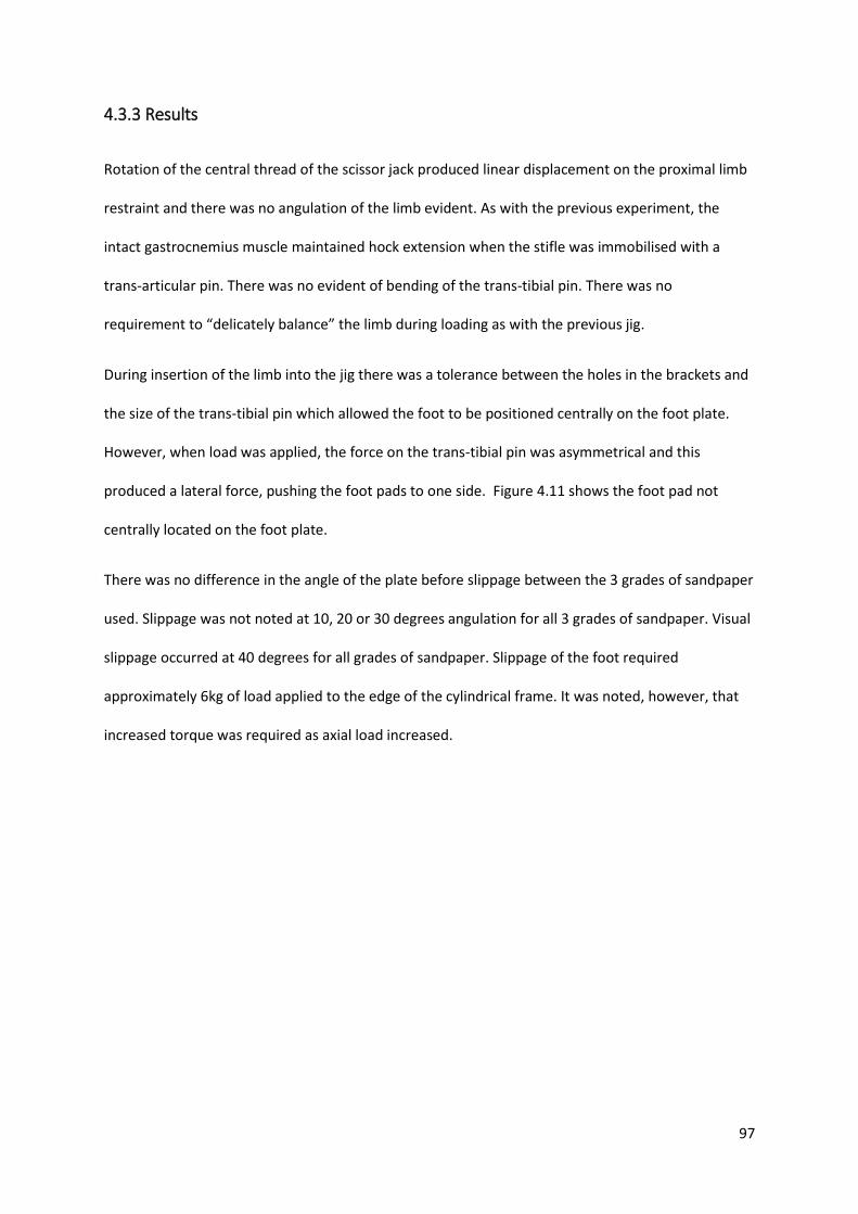
97

4.3.3 Results

Rotation of the central thread of the scissor jack produced linear displacement on the proximal limb

restraint and there was no angulation of the limb evident. As with the previous experiment, the

intact gastrocnemius muscle maintained hock extension when the stifle was immobilised with a

trans-articular pin. There was no evident of bending of the trans-tibial pin. There was no

requirement to “delicately balance” the limb during loading as with the previous jig.

During insertion of the limb into the jig there was a tolerance between the holes in the brackets and

the size of the trans-tibial pin which allowed the foot to be positioned centrally on the foot plate.

However, when load was applied, the force on the trans-tibial pin was asymmetrical and this

produced a lateral force, pushing the foot pads to one side. Figure 4.11 shows the foot pad not

centrally located on the foot plate.

There was no difference in the angle of the plate before slippage between the 3 grades of sandpaper

used. Slippage was not noted at 10, 20 or 30 degrees angulation for all 3 grades of sandpaper. Visual

slippage occurred at 40 degrees for all grades of sandpaper. Slippage of the foot required

approximately 6kg of load applied to the edge of the cylindrical frame. It was noted, however, that

increased torque was required as axial load increased.

98

4.3.4 Discussion

The second jig overcame the major limitations of the previous jig, namely, plastic deformation of the

trans-tibial pin and requirement for perfect “balance” to prevent angulation of the limb. During this

experiment, additional factors which required modification, were also identified.

• Inaccurate drilling of bone tunnel.

In this experiment, the bone tunnel was not directed in a perfectly orthogonal plane. In the previous

jig, this asymmetry was overcome by individual tensioning of a medial and lateral strap. However,

with jig 2, the orientation of the bone tunnel influenced the position of the foot on the foot plate.

The protocol was modified so that the limb was positioned into the proximal restraint before the

bone tunnel was drilled. This ensured the foot was in the optimal central position. The start point of

the bone tunnel was marked and a drill guide, which was attached to the restraint was developed

(figure 4.12).

• Replication of angle of foot plate

Positioning of wooden blocks under the footplate was convenient for the preliminary studies but

was considered an unreliable means to consistently reproduce foot plate angles. A radiolucent foot

plate constructed entirely of wood and plastic was developed at a set angle. The initial slope was set

Figure 4-12: A removable drill guide was developed to ensure the bone tunnel was directed orthogonally across the proximal tibia and would pass through the holes in the brackets. The bone tunnel was drilled with the limb positioned in the jig and metatarsal pad centered on the foot plate.

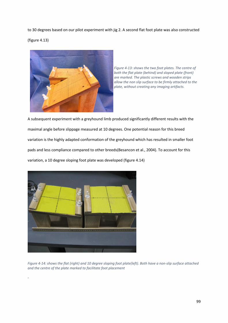
99

to 30 degrees based on our pilot experiment with jig 2. A second flat foot plate was also constructed

(figure 4.13)

A subsequent experiment with a greyhound limb produced significantly different results with the

maximal angle before slippage measured at 10 degrees. One potential reason for this breed

variation is the highly adapted conformation of the greyhound which has resulted in smaller foot

pads and less compliance compared to other breeds(Besancon et al., 2004). To account for this

variation, a 10 degree sloping foot plate was developed (figure 4.14)

Figure 4-14: shows the flat (right) and 10 degree sloping foot plate(left). Both have a non-slip surface attached and the centre of the plate marked to facilitate foot placement

.

Figure 4-13: shows the two foot plates. The centre of both the flat plate (behind) and sloped plate (front) are marked. The plastic screws and wooden strips allow the non slip surface to be firmly attached to the plate, without creating any imaging artifacts.

100

The foot plate was further refined by the introduction of a pivoting foot plate, that would allow

alteration in slope without the need to remove the foot off the plate (which may introduce

inaccuracy as the foot was replaced on the foot plate). Initially the angles were maintained by a

series of pegs (figure 4.15). This system was replaced with the final design of footplate which was

capable of an infinite number of slope angles. Alteration of the foot plate angle could be performed

by turning two screws positioned under the plate (figure 4.16).

Figure 4-15: A pivoting foot plate allows angulation without having to remove and replace the foot. The position of the foot plate was maintained with pegs (open arrows)

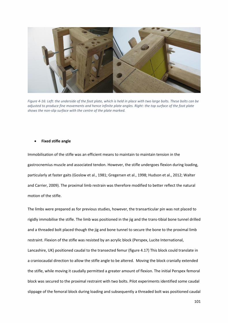
101

Figure 4-16: Left: the underside of the foot plate, which is held in place with two large bolts. These bolts can be adjusted to produce fine movements and hence infinite plate angles. Right: the top surface of the foot plate shows the non-slip surface with the centre of the plate marked.

• Fixed stifle angle

Immobilisation of the stifle was an efficient means to maintain to maintain tension in the

gastrocnemius muscle and associated tendon. However, the stifle undergoes flexion during loading,

particularly at faster gaits (Goslow et al., 1981; Gregersen et al., 1998; Hudson et al., 2012; Walter

and Carrier, 2009). The proximal limb restrain was therefore modified to better reflect the natural

motion of the stifle.

The limbs were prepared as for previous studies, however, the transarticular pin was not placed to

rigidly immobilise the stifle. The limb was positioned in the jig and the trans-tibial bone tunnel drilled

and a threaded bolt placed though the jig and bone tunnel to secure the bone to the proximal limb

restraint. Flexion of the stifle was resisted by an acrylic block (Perspex, Lucite International,

Lancashire, UK) positioned caudal to the transected femur (figure 4.17) This block could translate in

a craniocaudal direction to allow the stifle angle to be altered. Moving the block cranially extended

the stifle, while moving it caudally permitted a greater amount of flexion. The initial Perspex femoral

block was secured to the proximal restraint with two bolts. Pilot experiments identified some caudal

slippage of the femoral block during loading and subsequently a threaded bolt was positioned caudal

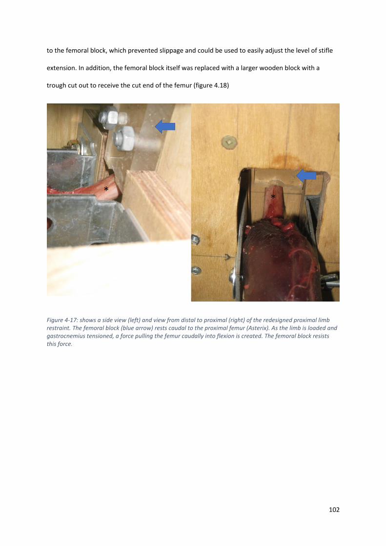
102

to the femoral block, which prevented slippage and could be used to easily adjust the level of stifle

extension. In addition, the femoral block itself was replaced with a larger wooden block with a

trough cut out to receive the cut end of the femur (figure 4.18)

Figure 4-17: shows a side view (left) and view from distal to proximal (right) of the redesigned proximal limb restraint. The femoral block (blue arrow) rests caudal to the proximal femur (Asterix). As the limb is loaded and gastrocnemius tensioned, a force pulling the femur caudally into flexion is created. The femoral block resists this force.

103

Figure 4-18: shows further modifications to the proximal limb restraint. The femoral block (blue arrow) positioned to resist stifle flexion is now larger and a bolt is positioned behind the block to prevent slippage of the block and permit easy alteration of femoral block position. A handle (open arrow) was secure to the end of the bolt to allow convenient adjustment to the craniocaudal position of the femoral block.

104

To evaluate if movement of the femoral block could alter the stifle angle, a greyhound cadaver limb

was prepared as described earlier. To identify the longitudinal axis of the femur, a 3mm diameter pin

was inserted from proximal to distal down the femoral medullary canal exciting distally through the

joint. Approximately 10cm of pin was left protruding from the joint to allow identification of the axis.

A 3mm diameter pin was inserted centrally in the distal tibia in a medial to lateral orientation to

mark the craniocaudal midpoint of the distal tibia. This point would mark the centre of the tibia

distally. The proximal trans-tibial pin was positioned just distal to the midpoint of the articular

surface of the tibial condyles and consequently a line connecting the proximal trans-tibial pin with

the distal tibial pin represented the tibial mechanical axis. The intersection of this line and the

femoral axis represented the stifle angle.

The limb was loaded with the femoral block positioned in its most caudal position. Digital

photographs were taken and the stifle angle measured using commercially available software (Image

J, https://imagej.net/Welcome). Without moving the position of the proximal limb restrain in the jig,

the femoral block was then moved to its most cranial position by turning the screw behind it. Digital

photographs were acquired and the stifle angle measured again (figure 4.19).

The stifle was extended from 98.1 degrees to 111.9 degrees with a set hock angle. With the ability to

alter stifle angle, the next experiment would validate the jig by comparing the stifle and hock angles

of the cadaver with previously published in vivo kinematic data. The final jig design can be seen in

figure 4.20.

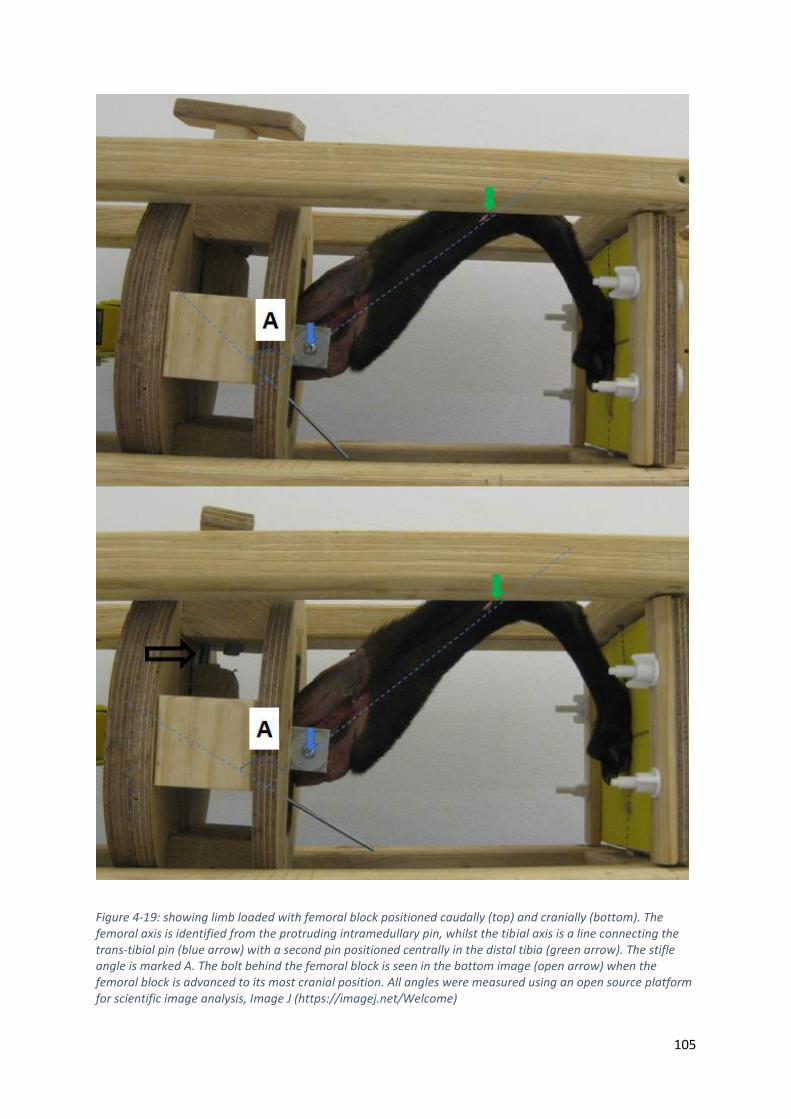
105

Figure 4-19: showing limb loaded with femoral block positioned caudally (top) and cranially (bottom). The femoral axis is identified from the protruding intramedullary pin, whilst the tibial axis is a line connecting the trans-tibial pin (blue arrow) with a second pin positioned centrally in the distal tibia (green arrow). The stifle angle is marked A. The bolt behind the femoral block is seen in the bottom image (open arrow) when the femoral block is advanced to its most cranial position. All angles were measured using an open source platform for scientific image analysis, Image J (https://imagej.net/Welcome)

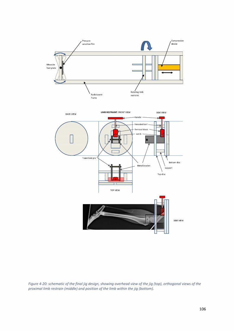
106

Figure 4-20: schematic of the final jig design, showing overhead view of the jig (top), orthogonal views of the proximal limb restrain (middle) and position of the limb within the jig (bottom).

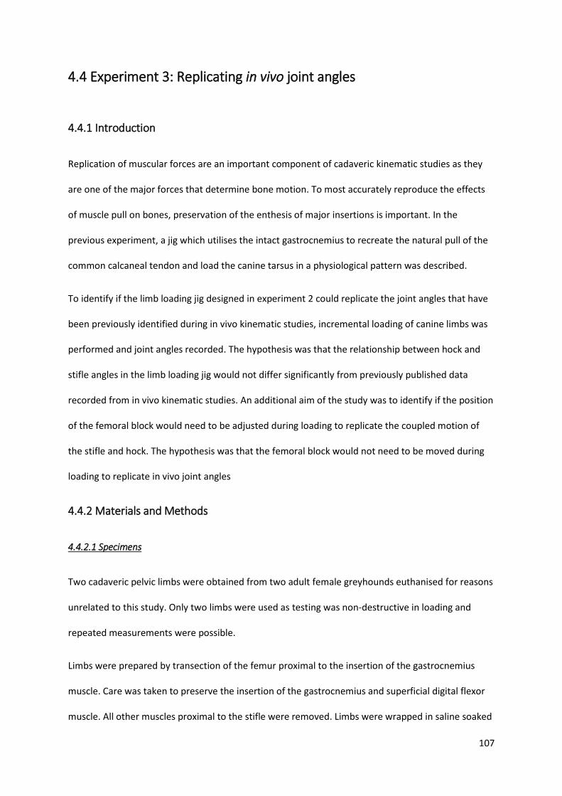
107

4.4 Experiment 3: Replicating in vivo joint angles

4.4.1 Introduction

Replication of muscular forces are an important component of cadaveric kinematic studies as they

are one of the major forces that determine bone motion. To most accurately reproduce the effects

of muscle pull on bones, preservation of the enthesis of major insertions is important. In the

previous experiment, a jig which utilises the intact gastrocnemius to recreate the natural pull of the

common calcaneal tendon and load the canine tarsus in a physiological pattern was described.

To identify if the limb loading jig designed in experiment 2 could replicate the joint angles that have

been previously identified during in vivo kinematic studies, incremental loading of canine limbs was

performed and joint angles recorded. The hypothesis was that the relationship between hock and

stifle angles in the limb loading jig would not differ significantly from previously published data

recorded from in vivo kinematic studies. An additional aim of the study was to identify if the position

of the femoral block would need to be adjusted during loading to replicate the coupled motion of

the stifle and hock. The hypothesis was that the femoral block would not need to be moved during

loading to replicate in vivo joint angles

4.4.2 Materials and Methods

4.4.2.1 Specimens

Two cadaveric pelvic limbs were obtained from two adult female greyhounds euthanised for reasons

unrelated to this study. Only two limbs were used as testing was non-destructive in loading and

repeated measurements were possible.

Limbs were prepared by transection of the femur proximal to the insertion of the gastrocnemius

muscle. Care was taken to preserve the insertion of the gastrocnemius and superficial digital flexor

muscle. All other muscles proximal to the stifle were removed. Limbs were wrapped in saline soaked

108

cloth to prevent tissue desiccation and frozen at -20 degrees until use. Limbs were thawed at 4

degrees overnight prior to use.

To identify the longitudinal axis of the femur, a 3mm diameter pin was inserted from proximal to

distal down the femoral medullary canal exciting distally through the joint. Approximately 10cm of

pin was left protruding from the joint to allow identification of the axis. A 3mm diameter pin was

inserted centrally in the distal tibia in a medial to lateral orientation to mark the craniocaudal

midpoint of the distal tibia. This point would mark the centre of the tibia distally. The proximal trans-

tibial pin was positioned just distal to the midpoint of the articular surface of the tibial condyles and

consequently a line connecting the proximal trans-tibial pin with the distal tibial pin represented the

tibial mechanical axis. The intersection of this line and the femoral axis represented the stifle angle.

The dorsal cortical border of the metatarsals was used to represent the axis of the pes. The

intersection of this line with the mechanical axis of the tibia produced the angle of the hock joint.

4.4.2.2 Mechanical loading

Limb 1 was initially loaded with the stifle in a more flexed position (femoral block caudally located).

Incremental loading was performed and angles of the stifle and hock measured when the linear

distance from the proximal restraint to the foot plate was 35cm, 33cm, 31cm and 29 cm. Digital

photographs were obtained and the angles measured using commercial software with a measuring

function (image J, (https://imagej.net))

The femoral block was then moved into the most cranial position (stifle extended) and stifle and

hock angle measurements were repeated at the same linear displacement (figure 4.21). During

incremental loading, there was no change to the position of the femoral block.

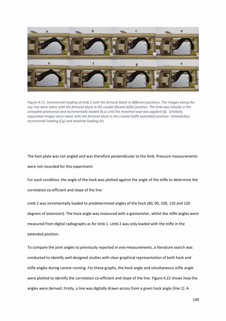
109

Figure 4-21: Incremental loading of limb 1 with the femoral block in different positions. The images along the top row were taken with the femoral block in the caudal (flexed stifle) position. The limb was initially in the unloaded position(a) and incrementally loaded (b,c) until the maximal load was applied (d). Similarly, sequential images were taken with the femoral block in the cranial (stifle extended) position. Unloaded(e), incremental loading (f,g) and maximal loading (h).

The foot plate was not angled and was therefore perpendicular to the limb. Pressure measurements

were not recorded for this experiment

For each condition, the angle of the hock was plotted against the angle of the stifle to determine the

correlation co-efficient and slope of the line

Limb 2 was incrementally loaded to predetermined angles of the hock (80, 90, 100, 110 and 120

degrees of extension). The hock angle was measured with a goniometer, whilst the stifle angles were

measured from digital radiographs as for limb 1. Limb 2 was only loaded with the stifle in the

extended position.

To compare the joint angles to previously reported in vivo measurements, a literature search was

conducted to identify well designed studies with clear graphical representation of both hock and

stifle angles during canine running. For these graphs, the hock angle and simultaneous stifle angle

were plotted to identify the correlation co-efficient and slope of the line. Figure 4.22 shows how the

angles were derived. Firstly, a line was digitally drawn across from a given hock angle (line 1). A

a c d b

h g f e

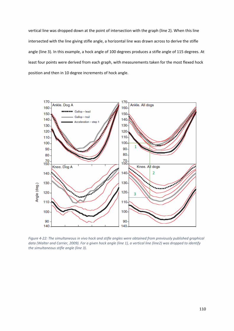
110

vertical line was dropped down at the point of intersection with the graph (line 2). When this line

intersected with the line giving stifle angle, a horizontal line was drawn across to derive the stifle

angle (line 3). In this example, a hock angle of 100 degrees produces a stifle angle of 115 degrees. At

least four points were derived from each graph, with measurements taken for the most flexed hock

position and then in 10 degree increments of hock angle.

Figure 4-22: The simultaneous in vivo hock and stifle angles were obtained from previously published graphical data (Walter and Carrier, 2009). For a given hock angle (line 1), a vertical line (line2) was dropped to identify the simultaneous stifle angle (line 3).

111

4.4.3 Results

The joint angles for the stifle and hock of the cadaver limbs were recorded (Table 4.1). Limb 1 was

incrementally loaded by linear distance from proximal restraint to foot plate whilst limb 2 was

loaded to a set hock angle.

There was high correlation between stifle and hock angles (fig 4.23) for all cadaveric limbs.

Table 4-1: The hock and stifle angles of the two cadaver limbs in this study. Limb one was tested with the femoral block in a “stifle flexed” and “stifle extended” position. For all limbs, the reduction in hock angle that occurred during loading was also associated with a reduction in stifle angle

Limb Limb 1 Limb 2

stifle position stifle flexed stifle extended stifle extended

Joint stifle angle hock angle stifle angle hock angle stifle angle hock angle

angle (degrees)

111.1 112.96 139 114.33 140.7 120

103.6 99.2 131.6 99.88 127.6 110

100.8 89.7 125.5 90.2 123.5 100

95.3 82.8 119.3 79.56 118.6 90

115.0 80

112

Figure 4-23: The correlation of stifle and hock angles for limb one with the stifle in a flexed (left) or extended(right) position. A trendline and value for correlation are seen, along with the slope of the line.

Two studies with clear graphs that would allow us to plot stifle vs hock angles were identified

(Walter and Carrier 2009, Gregersen et al. 1998). An example of a graph is seen below (Fig 4.24) and

a summary table comparing the results from the cadaver study to previously published in vivo

results (table 4.2)

Figure 4-24: Plotted stifle and hock angles for the lead hind leg (left) and trailing leg (right) from Walter and Carrier (2009)

y = 1.9654x - 105.68R² = 0.9794

0

20

40

60

80

100

120

90 95 100 105 110 115

Ho

ck a

ngl

e (d

egre

es)

Stifle angle (degrees)

Limb 1: Stifle flexed position

y = 1.7518x - 129.73R² = 0.9981

0

20

40

60

80

100

120

140

110 120 130 140

Ho

ck a

ngl

e (d

egre

es)

Stifle angle (degrees)

Limb 1: Stifle extended position

y = 1.9959x - 153.06R² = 0.9858

0

20

40

60

80

100

120

140

120 125 130 135 140 145

Ho

ck a

ngl

e (d

egre

es)

Stifle angle (degrees)

Walter and Carrier 2009 Stifle Vs Hock angle in the

lead limb

y = 1.4061x - 61.749R² = 0.9875

0

20

40

60

80

100

120

140

100 110 120 130 140

Ho

ck a

ngl

e (d

egre

es)

Stifle angle (degrees)

Walter and Carrier 2009 Stifle Vs Hock angle in the

trailing limb

113

Table 4-2: The correlation co-efficient and slope from the cadavers used in this experiment and three previous in vivo kinematic studies when stifle and hock angle are plotted against each other. A correlation coefficient of 1 represents a perfect linear relationship, whilst 0 represents random data. All limbs in the above table show a near perfect linear relationship between stifle and hock angles. The coupling ratio represents the slope of the trendline. A coupling ratio of 1 means that for every one degree of stifle flexion, one degree of hock flexion occurs. A coupling ratio of 2 means that for every one degree of stifle flexion, two degrees of hock flexion occurs.

study correlation

co-efficient

Coupling

ratio

Limb 1: stifle flexed

position 0.9794 1.965

Limb 1: stifle extended

position 0.9981 1.752

Limb 2: Stifle extended

position 0.9191 1.521

Walter and Carrier 2009:

Dog A lead leg 0.9934 1.996

Walter and Carrier 2009:

Dog A trailing leg 0.9987 1.406

Gregerson 1998 0.9946 2.783

In vivo studies, show a very high correlation between stifle and hock angles in galloping dogs. The

slope of the trendlines ranges from 1.406 to 2.783, meaning that for every 1 degree of stifle flexion

there is 1.406 to 2.783 degrees of hock flexion. The cadavers loaded in our jig also showed a very

high correlation, with R2 values all >0.9 and slope ranging from 1.521 to 1.965, which is within the

range from the in vivo studies. The values from Gregerson (1998) are obtained from non weight

bearing limbs in comparison to the loaded limbs from Walter and Carrier (2009).

114

4.4.4 Discussion

The results of this study demonstrate that the angles of the stifle and hock in our cadaver limb

loading jig are highly correlated, with every 1 degree of stifle flexion producing between 1.521 and

1.965 degrees of tarsal flexion. The coupled motion of the stifle and hock was also identified in

previously published in vivo studies, where 1 degree of stifle flexion produced between 1.406 and

2.783 of tarsal flexion (Walter and Carrier 2009, Gregersen et al. 1998). The results from the

cadaveric limbs fall within the ranges previously recorded in vivo, therefore supporting the

hypothesis that the limb loading jig being evaluated is capable of replicating in vivo joint angles.

The position of the femoral block did influence the relationship between stifle and hock angles but

this relationship (slope of the line when stifle angle and hock angle are plotted against each other)

remained within the limits of previous in vivo testing, suggesting either position would be

appropriate for replicating in vivo joint angles.

Coupling of stifle and hock flexion has been previously described with 1 degree of stifle flexion

resulting in 0.72 degrees of hock flexion (Gregersen et al., 1998). That is, a change in stifle angle

produces a smaller change in hock angle. This is in contrast to the present cadaveric study and in

vivo measurements, where the change in stifle angle produced a greater change in hock angle. This

can be explained by the measurement techniques used in both studies. Gregerson et al (1998)

measured these angles in non-weight bearing limbs, whilst our measurements and those from in

vivo studies were measured during loading of the limb. Elasticity in the gastrocnemius tendon allows

an increased degree of hock flexion during load bearing as is considered the most likely reason for

these discrepancies.

The length of the gastrocnemius increases during the stance phase by up to 10% (Goslow et al.,

1981) despite activation of the muscle. The muscle fibre length and pennate arrangement of the

gastrocnemius suggest this muscle undergoes isometric contraction and comprises part of the

biological spring mechanism of the limb.

115

In this experiment, the force exerted by the foot pads on the foot plate was not recorded, which

would have allowed correlation between limb angles and applied force, further validating the use of

this device.

Although this limb loading device accurately replicates the coupled motion of the stifle and hock,

further studies that measure the force exerted by the foot are required before the jig can be

validated as accurately replicating the biomechanics of the distal limb.

116

4.5 Experiment 4: Replication of joint forces

4.5.1 Introduction

During force-displacement studies, the investigator may choose to load to a set displacement (and

measure force) or alternatively load to a predetermined force (and measure displacement). In the

previous experiment, displacement of the limb segments, and subsequent joint angles were

recorded, however, the force exerted on the limb was not measured. To investigate if the force

exerted on the foot plate is within physiological limits for a given displacement, the jig was modified

to allow quantification of the force the paw exerts on the foot plate. The angle of flexion of the hock

when loaded to a predetermined force on the foot plate is reported in the following experiment.

4.5.2 Materials and Methods

To enable the measurement of force transmitted through the limb, pressure sensitive film (Film code

5076-350. Tekscan, South Boston, MA, USA ) was positioned under the non-slip surface of the foot

plate. The film was calibrated to measure force in newtons. The readout produced a real-time

pattern of loading of the foot pads and the peak force measured (figure 4.25).

10 paired canine cadaver hind limbs from adult greyhounds euthanised for reasons unrelated to this

study were obtained. They were prepared and positioned into the limb loading jig as described for

the previous experiment.

The limbs were loaded until the peak vertical force reached 600N, which is approximately 1.7 X body

weight for an average greyhound. This value was selected based on recordings of peak vertical force

of the hind limbs of a galloping dog. (Walter and Carrier, 2007; Walter and Carrier, 2009)

The jig and attached limb were then scanned in a computed tomography scanner (Philips Brilliance

16-slice CT scanner)(120KVP, 117 mA, slice thickness 1mm, slice increment 0.5mm, 512 X512matrix).

117

The DICOM images imported into commercially available software (Mimics 17.0, Materialize,

Belgium)

From sagittal images, the angle of hock flexion was recorded. A line was drawn between the tibial

tuberosity and the centre of the talus. A second line connected the centre of the talus to the

metatarsophalyngeal joint. The intersection of these lines gave the joint angle (fig 4.26). These

landmarks do not represent the mechanical long axis of the bones but correlate with the position of

skin markers used in previous kinematic studies.

Figure 4-25: The pressure sensitive film being positioned under the non-slip surface (left). The foot was centred on the foot plate (right) and a digital pressure distribution pattern produced (inset). This film allowed real time recording of force exerted as well as the distribution of load through the digital and metatarsal pads. Additionally, the centre of force distribution is also recorded and was shown to move caudally during limb loading.

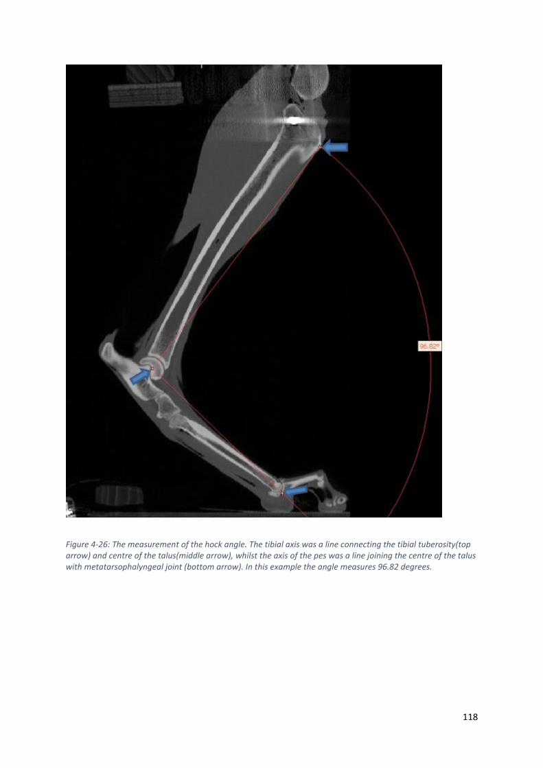
118

Figure 4-26: The measurement of the hock angle. The tibial axis was a line connecting the tibial tuberosity(top arrow) and centre of the talus(middle arrow), whilst the axis of the pes was a line joining the centre of the talus with metatarsophalyngeal joint (bottom arrow). In this example the angle measures 96.82 degrees.

119

4.5.3 Results

The mean angle and hock flexion was 101.0 ± 7.33 degrees when 600N was recorded on the

pressure sensitive film. The results of the individual limbs can be seen in table 4.3

Table 4-3 hock angle of the 10 specimens when a peak vertical force of 600N was recorded. The mean hock angle of 101 degrees is similar to in vivo measurements from previous investigations which simultaneously recorded ground reaction force and joint angles using skin markers (Walter and Carrier, 2007)

Specimen

number

hock angle

(degrees)

1 95.87

2 101.97

3 96.25

4 96.61

5 89.59

6 96.82

7 114.7

8 107.44

9 105.37

10 105.37

mean 101.00

SD 7.33

120

4.5.4 Discussion

A mean hock angle of 101 ± 7.33 degrees was recorded when the ground reaction force of

approximately 1.7 X body weight was applied. This finding is consistent with the minimum angle of

hock flexion (96 ± 8.8 for the lead hind limb and 97 ± 3.8 for the trailing hind limb) recorded in vivo,

which simultaneously produced a peak vertical force of 1.64 ± 0.11 X body weight in the galloping

dog(Walter and Carrier, 2009). These findings support the hypothesis that the limb loading jig can

produce a hock flexion angle and ground reaction force similar to those recording from the in vivo

galloping dog.

The ground reaction force(GRF) is dependent on a tensile force being applied to the tuber calcanei.

(fig 4.27) The magnitude of the GRF will increase if tensile forces acting on the calcaneus increase

and conversely, the GRF will decrease if the tensile force decreases.

121

In the limb loading jig, designed to simulate both internal and external forces across the tarsus, the

tensile force acting on the tuber calcanei is produced by the intact gastrocnemius. Despite no active

contraction of the muscle in the cadaver specimen, this muscle is still able to generate a tensile fore

on the calcaneus when the stifle is prevented from flexing. The m. gastrocnemius is covered in thick

tendinous leaves and is infiltrated by tendinous strands(Evans et al., 2012). Previous investigations of

the canine gastrocnemius suggest that is a major contributor to the biological spring of the hind

limb, with a high tendon length change: muscle fascicle length, indicating a reliance on passive

length change (tendon elongation) rather than active muscle shortening (Williams et al., 2009). In

vivo studies report a lengthening of the gastrocnemius of 9% during the first stages of the stance

phase, followed by a 10% shortening at take-off , suggesting that active contraction of the muscle is

most important in the final stages of the stance phase (Goslow et al., 1981).

Figure 4-27: shows the forces acting on the canine pes. The pes will rotate about the centre of the talus, which is loaded by the animal’s body weight (blue arrow). A tensile force produced by the gastrocnemius (green arrow) will produce a proportional ground reaction force that can be measured using the pressure sensitive film (open yellow arrow)

122

Accurately reproducing the stifle and hock angles during loading is likely to result in a close

approximation of the tensile force within the gastrocnemius muscle and tendon that occur during

galloping. This in turn, has produced a ground reaction force that is comparable to measurements

made in galloping dogs.

This limb loading jig can accurately reproduce the displacement of limb segments during loading

(measured by stifle and hock angles) and accurately reproduced the major internal and external

forces exerted on the tarsus, including replication of the major muscular forces exerted during

weight bearing at high speeds. These findings suggest that this limb loading jig would be able to

accurately reproduce in vivo tarsal kinematics for a dog running at high speeds. However, it must be

recognised that the rate of loading in this jig occurs slowly in contrast to in vivo conditions where the

stance phase may be a short as 0.2 seconds during trotting. As tissues of the musculoskeletal system

are viscoelastic, this is, will demonstrate different material properties dependant on the rate of

loading, any difference in loading rate may influence any potential results.

123

4. 6 Chapter discussion

A radiolucent limb loading jig that can replicate the coupled motion of the hock and stifle as

observed in in vivo studies (Goslow et al., 1981; Gregersen et al., 1998; Walter and Carrier, 2009)

and the internal and external forces that are exerted on the canine tarsus during high speed running

was designed, constructed and further refined as part of this thesis.

This jig was designed with the purpose of investigating canine tarsal bone kinematics using non-

invasive CT based kinematic measurements. Prior to construction, a number of key capabilities that

would be required from such a device were identified.

Firstly, the jig would have to be constructed of radiolucent material in the areas where metal

artefact may interfere with identifying the cortical contours of the tarsal bones. This jig was

constructed primarily with pine which has a radiographic density of -456 Hounsfield Units (HU) (Lee,

2010), which is well below the density of water (0HU) and bone (greater than700 HU) (Fat et al.,

2012). During processing of the DICOM images, the only artefacts were created by the metal

brackets used to restrain the proximal limb. No artefacts were identified at the level of the tarsal

bones.

Secondly, the jig was designed to approximate in vivo loads and permit kinematic measurements

with minimal disruption to the tissues. All cadaver limbs were frozen before use and dehydration

was prevented by wrapping limbs in saline soaked cloth. Previous studies have suggested that the

material properties of connective tissue are minimally affected by the freezing process (Moon et al.,

2006; Woo et al., 1986).

Maintaining the soft tissue structures that surround joints is important for accurate recreation of

forces when using cadaver models as the ligaments and joint capsule act as natural passive restraints

to limit motion. The loading jig described in this chapter required no dissection distal to the mid tibia

for loading or kinematic measurements, allowing preservation of all periarticular structures.

124

Recreation of muscular force is essential when studying kinematics in cadaver models as the

magnitude and direction of muscular tensile forces determine the displacement of bone, in

conjunction with the limiting effects of ligaments, joint capsule and congruent bone contours. The

canine tarsal bones have few direct muscular attachments. The common calcaneal tendon inserts

upon the tuber calcanei and comprises the tendons of the superficial digital flexor muscle,

gastrocnemius muscle and conjoined tendon of gracillis, semitendinosis and biceps femoris. In this

model, preservation of the superficial digital flexor and gastrocnemius muscles allowed accurate

recreation of tensile force (experiment 4.4). Both these muscles show a high tendon length change:

muscle fascicle length, indicating a reliance on passive length change (tendon elongation) rather

than active muscle shortening(Williams et al., 2009).

The other muscle with direct insertion on the tarsal bones is the cranial tibial muscle, a flexor of the

hock that is not active during mid stance and hence no attempt was made to replicate the force

produced by this muscle. Other tarsal flexors include the fibularis longus and fibularis brevis which

are both active in the swing phase of gait (Wentink, 1976) but not active during the stance phase.

The quadratus plantae muscle is considered an insignificant muscle running from the lateral

tuberosity of the calcaneus to the deep digital flexor tendon (Evans et al., 2012).

The extensor digitorum brevis has its origin on the dorsal part of the calcaneus and runs distally. This

small muscle extends the digits and is not considered active during the stance phase(Evans et al.,

2012) and hence, no attempt was made to replicate its effect.

The adductor digit V is a small, mainly tendinous muscle that runs from the lateral aspect of the

tuber calcanei to insert of the base of metatarsal V (Evans et al., 2012). This mainly tendinous band

was preserved allowing replication of the passive effects of the muscle.

The gastrocnemius spans across two joints and couples the motion of the stifle and hock joints. The

relationship between stifle and hock flexion differs between the passive range of motion (without

125

weight bearing load) and load bearing scenarios. Whilst one degree of stifle flexion results in less

than 1 degree of hock flexion in the non-load bearing state, one degree of stifle flexion during load

bearing produces greater than one degree of flexion at the hock joint. This finding may be partially

explained by the elongation in the gastrocnemius muscle which has been previously reported

(Alexander, 2002), but another possible explanation is dorsiflexion of the pes. In other species, up to

17 degrees of dorsiflexion was observed at the intertarsal and tarsometatarsal joints. It is likely that

both factors are responsible for the observed changes in stifle and hock coupling.

The initial limb loading jig design relied upon immobilisation of the stifle joint and prevented

simultaneous flexion of the stifle and hock as seen in in in vivo kinematic studies. Following

modification of the proximal limb restraint, the coupled motion of the stifle and hock that has been

identified in vivo, was reproduced.

Limitations:

This series of experiments represents the evolution of the limb loading device, which developed

rapidly following each experiment. Therefore, large numbers of replicates were not performed for

every step as obvious flaws were identified and rectified. All testing was non-destructive and so

allowed for repeated measures to be performed on single specimens. However, there is the

possibility of changes to the material properties of the limb with repeated loading due to tissue

creep, which may not be recoverable in cadaveric tissue, and has the potential to influence results.

The load exerted on the force plate as the limb was repeatedly loaded and unloaded to the same

position in the jig was measured and noted that after 1-2 cycles, there was no change in force

recorded for the following measurements. Although this data is not reported here, it was used to

develop the pre-conditioning protocol that was used in later experiments.

The data from the cadaveric specimen was only compared to in vivo data from a limited number of

dogs from previous studies (Gregersen et al., 1998; Walter and Carrier, 2009). These studies were

selected as they provided clear graphical representation that allowed us to derive simultaneous hock

126

and stifle angles from in vivo experiments. Other studies (Goslow et al., 1981), also represent similar

graphical data but the image resolution was not of a suitable standard to reliable derive the required

data. It is important to acknowledge that small errors are possible when deriving numerical data

from published graphical representations rather than the original data set.

Validation of this jig could also include instrumenting tendons and ligaments, such as the common

calcaneal tendon and plantar ligament, with strain gauges allowing comparisons to be made to the

in vivo scenario. Similarly, direct measurement of forces across the individual joints could have been

performed with pressure sensitive film and used as another validation measure. This was not

performed in this series of experiments for two reasons; firstly, it would involve performing a series

of in vivo experiments as there is no published data recording the strain in these tissues for canine

limbs or force across articular surfaces during high speed running in the dog. Secondly,

instrumentation with strain gauges and pressure sensitive films would require further dissection of

the pes, which may alter the kinematic patterns of the bones being investigated. Rather, the

resultant force on the ground, measurement of elongation of the gastrocnemius muscle and joint

angles were used as in vivo data was available for these parameters to allow a comparison to be

made and measurements could be recorded without disrupting tissues, such as the tendons,

ligaments and joint capsules, which all play a role in determining bone kinematics. However, it is

acknowledged that direct measurement of internal forces in the cadaveric limb and comparison to in

vivo data would provide further validation of this jig and its ability to replicate all relevant forces for

the weight bearing limb.

Conclusion

The results of the experiments performed in this chapter suggest the limb loading jig can accurately

replicate the displacement of limb segments and produce ground reaction force comparable to in

vivo kinetic and kinematic studies. As most of the forces on the tarsal bones are passive, derived

from the forces from adjacent bones, the joint capsule and ligaments, the ability of this jig to

127

accurately replicate the internal forces of the tarsus without dissection of the distal limb makes it a

valuable device for the study of tarsal bone kinematics.

The overall design of this jig may also make it suitable for investigating bone kinematics in the canine

forelimb and in the limbs of other digitigrade species. Modifications to the proximal limb restrain

may be required but the development of a range of proximal limb restraints may increase the

versatility of this jig and scope for kinematic investigations.

128

Chapter 5 : Characterisation of canine

tarsal bone kinematics identifies the

functional units of the canine foot

129

5.1 Introduction

The limbs of trotting, galloping or hopping terrestrial mammals can be considered as biological

springs, storing kinetic and potential energy as elastic strain during the first half of the stance phase,

then releasing this energy as the animal propels itself upwards and forwards during the second half

on the stance phase of gait (Alexander and Bennet-Clark, 1977). It has been suggested that this

mechanism may conserve up to 50% of the energy that would otherwise be required did this

mechanism not exist (Alexander and Vernon, 1975; Cavagna et al., 1964).

The mechanism that facilitates energy storage is complex and remains only partially characterized in

most species. It involves a highly specific anatomical arrangement of tissues with varying mechanical

properties and will naturally vary between animals with different conformation and gait.

Amongst legged terrestrial animals, the dog (Canine Familiaris) is a supreme athlete capable of both

great speed and endurance (Poole and Erickson, 2011). In this species, the majority of energy

storage in the hind limb occurs below the stifle due to the specific arrangement of tissues with

differing mechanical properties (Alexander, 1984; Gregersen et al., 1998). In common with other

species, the larger muscles of the thigh have long muscle fibres and short tendons (Williams et al.,

2008), which facilitates active muscle shortening but limits their able to store elastic strain

(Alexander, 1984). In contrast, the muscles of the crus display short fibres in a pennate arrangement

with elongated tendons; an arrangement which facilitates elastic strain storage (Alexander, 1984;

Alexander and Bennet-Clark, 1977). Active muscle shortening does not appear to contribute

significantly to generating elastic strain in elongated tendons, but rather a change in joint angle leads

to stretching of these tendons. This is observed at the hock, when flexion of this joint during the

stance phase results in elongation of the gastrocnemius muscle, the primary extensor of the hock.

The gastrocnemius muscle and tendon, will lengthen by up to 9% during eccentric contraction during

the stance phase (Goslow et al., 1981), allowing storage of significant amount of elastic strain

energy. In addition, hock flexion will also result in lengthening of the digital flexor tendons as they

130

pass along the caudal aspect of the joint, further facilitating the storage of elastic stain energy in the

distal limb.

Elastic deformation of the pes has been documented in a number of species including man (Ker et

al., 1987) and camels (Alexander et al., 1982) and is believed to further contribute to elastic energy

storage in the limb. In camels, up to 17 degrees of dorsiflexion occurred at the intertarsal and

tarsometatarsal joints and this motion allowed greater elongation of flexor tendons and hence,

energy storage (Alexander et al., 1982). In the human foot, the flattening of the longitudinal arch

stretches connective tissue of the foot and has been shown to store about half the elastic strain that

can is stored in the Achilles tendon, further improving locomotor efficiency (Ker et al., 1987).

The canine pes is commonly modelled as a rigid structure in kinematic studies (Fischer and Blickhan,

2006; Fu et al., 2010; Gregersen et al., 1998; Hottinger et al., 1996; Walter and Carrier, 2009), which

allows application of the laws of rigid body mechanics and generates clinical useful information

regarding gait (Colborne et al., 2005; Colborne et al., 2006). However, the canine pes comprises 7

tarsal bones (talus, calcaneus, central, fourth, third, second and first tarsal bones) four metatarsals

and the phalanges (figure 5.1). Palpable motion is recognised at the intertarsal and tarsometatarsal

joints, with these joints described as low motion joints (Gorse et al., 1990) and exceedingly rigid

(Evans et al., 2012). The magnitude, direction and significance of intertarsal bone motion is

currently unknown, however, it can be hypothesised that intertarsal bone motion facilitates

dorsiflexion of the pes during locomotion, which may enhance the ability to store elastic strain

energy in structures such as the digital flexor tendons and plantar ligaments.

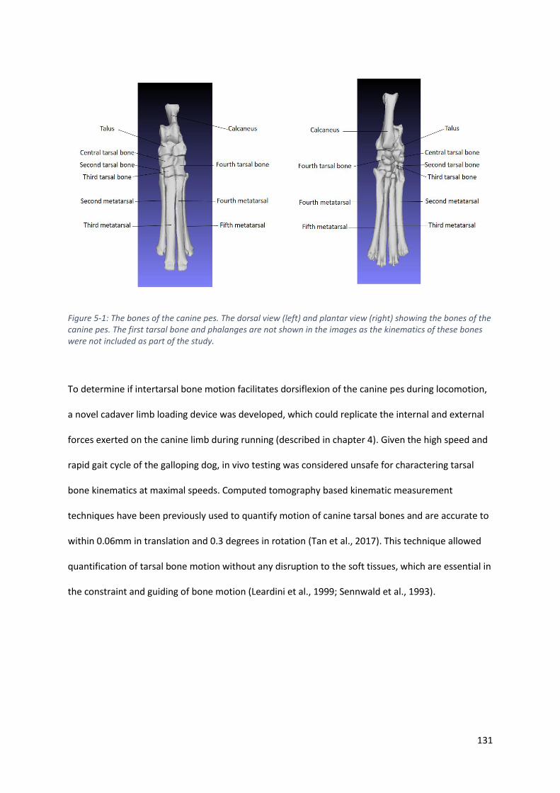
131

Figure 5-1: The bones of the canine pes. The dorsal view (left) and plantar view (right) showing the bones of the canine pes. The first tarsal bone and phalanges are not shown in the images as the kinematics of these bones were not included as part of the study.

To determine if intertarsal bone motion facilitates dorsiflexion of the canine pes during locomotion,

a novel cadaver limb loading device was developed, which could replicate the internal and external

forces exerted on the canine limb during running (described in chapter 4). Given the high speed and

rapid gait cycle of the galloping dog, in vivo testing was considered unsafe for charactering tarsal

bone kinematics at maximal speeds. Computed tomography based kinematic measurement

techniques have been previously used to quantify motion of canine tarsal bones and are accurate to

within 0.06mm in translation and 0.3 degrees in rotation (Tan et al., 2017). This technique allowed

quantification of tarsal bone motion without any disruption to the soft tissues, which are essential in

the constraint and guiding of bone motion (Leardini et al., 1999; Sennwald et al., 1993).

132

The aims of this study were to:

• Characterise the motion of each canine tarsal bone within a 3-dimensional, anatomically

based reference frame

• Describe how intertarsal bone motion may contribute to elastic deformation of the pes,

quantifying the contribution of motion within the pes to overall hock flexion

• Identify if any co-ordinated pattern of intertarsal bone motion occurs by identifying both

rigid functional units and highly correlated, kinematically coupled movements.

The first hypothesis was that tarsal bone motions does not occur simply in the sagittal plane and

more complex out of plane motions are also involved for each bone. The second hypothesis to be

tested was that dorsiflexion of the pes occurs during weight bearing making an overall contribution

to hock flexion. The final hypothesis was that within the tarsal and metatarsal bones, there will be

pairs of bones that move in unison allowing us to consider them as a rigid functional unit.

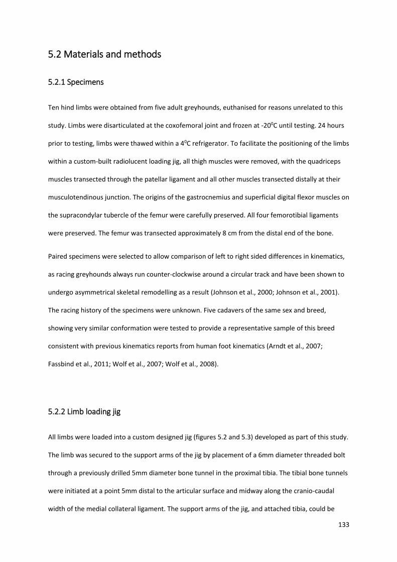
133

5.2 Materials and methods

5.2.1 Specimens

Ten hind limbs were obtained from five adult greyhounds, euthanised for reasons unrelated to this

study. Limbs were disarticulated at the coxofemoral joint and frozen at -200C until testing. 24 hours

prior to testing, limbs were thawed within a 40C refrigerator. To facilitate the positioning of the limbs

within a custom-built radiolucent loading jig, all thigh muscles were removed, with the quadriceps

muscles transected through the patellar ligament and all other muscles transected distally at their

musculotendinous junction. The origins of the gastrocnemius and superficial digital flexor muscles on

the supracondylar tubercle of the femur were carefully preserved. All four femorotibial ligaments

were preserved. The femur was transected approximately 8 cm from the distal end of the bone.

Paired specimens were selected to allow comparison of left to right sided differences in kinematics,

as racing greyhounds always run counter-clockwise around a circular track and have been shown to

undergo asymmetrical skeletal remodelling as a result (Johnson et al., 2000; Johnson et al., 2001).

The racing history of the specimens were unknown. Five cadavers of the same sex and breed,

showing very similar conformation were tested to provide a representative sample of this breed

consistent with previous kinematics reports from human foot kinematics (Arndt et al., 2007;

Fassbind et al., 2011; Wolf et al., 2007; Wolf et al., 2008).

5.2.2 Limb loading jig

All limbs were loaded into a custom designed jig (figures 5.2 and 5.3) developed as part of this study.

The limb was secured to the support arms of the jig by placement of a 6mm diameter threaded bolt

through a previously drilled 5mm diameter bone tunnel in the proximal tibia. The tibial bone tunnels

were initiated at a point 5mm distal to the articular surface and midway along the cranio-caudal

width of the medial collateral ligament. The support arms of the jig, and attached tibia, could be

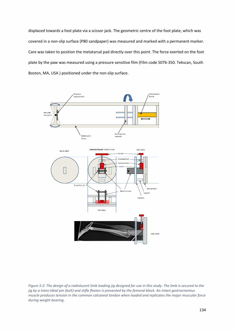
134

displaced towards a foot plate via a scissor jack. The geometric centre of the foot plate, which was

covered in a non-slip surface (P80 sandpaper) was measured and marked with a permanent marker.

Care was taken to position the metatarsal pad directly over this point. The force exerted on the foot

plate by the paw was measured using a pressure sensitive film (Film code 5076-350. Tekscan, South

Boston, MA, USA ) positioned under the non-slip surface.

Figure 5-2: The design of a radiolucent limb loading jig designed for use in this study. The limb is secured to the jig by a trans-tibial pin (bolt) and stifle flexion is prevented by the femoral block. An intact gastrocnemius muscle produces tension in the common calcaneal tendon when loaded and replicates the major muscular force during weight bearing.

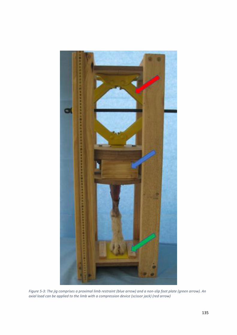
135

Figure 5-3: The jig comprises a proximal limb restraint (blue arrow) and a non-slip foot plate (green arrow). An axial load can be applied to the limb with a compression device (scissor jack) (red arrow)

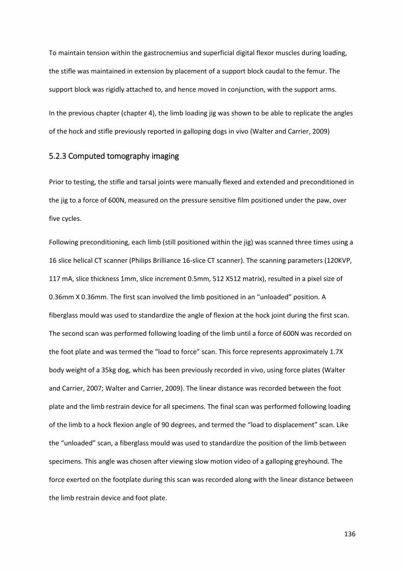
136

To maintain tension within the gastrocnemius and superficial digital flexor muscles during loading,

the stifle was maintained in extension by placement of a support block caudal to the femur. The

support block was rigidly attached to, and hence moved in conjunction, with the support arms.

In the previous chapter (chapter 4), the limb loading jig was shown to be able to replicate the angles

of the hock and stifle previously reported in galloping dogs in vivo (Walter and Carrier, 2009)

5.2.3 Computed tomography imaging

Prior to testing, the stifle and tarsal joints were manually flexed and extended and preconditioned in

the jig to a force of 600N, measured on the pressure sensitive film positioned under the paw, over

five cycles.

Following preconditioning, each limb (still positioned within the jig) was scanned three times using a

16 slice helical CT scanner (Philips Brilliance 16-slice CT scanner). The scanning parameters (120KVP,

117 mA, slice thickness 1mm, slice increment 0.5mm, 512 X512 matrix), resulted in a pixel size of

0.36mm X 0.36mm. The first scan involved the limb positioned in an “unloaded” position. A

fiberglass mould was used to standardize the angle of flexion at the hock joint during the first scan.

The second scan was performed following loading of the limb until a force of 600N was recorded on

the foot plate and was termed the “load to force” scan. This force represents approximately 1.7X

body weight of a 35kg dog, which has been previously recorded in vivo, using force plates (Walter

and Carrier, 2007; Walter and Carrier, 2009). The linear distance was recorded between the foot

plate and the limb restrain device for all specimens. The final scan was performed following loading

of the limb to a hock flexion angle of 90 degrees, and termed the “load to displacement” scan. Like

the “unloaded” scan, a fiberglass mould was used to standardize the position of the limb between

specimens. This angle was chosen after viewing slow motion video of a galloping greyhound. The

force exerted on the footplate during this scan was recorded along with the linear distance between

the limb restrain device and foot plate.

137

5.2.4 Bone segmentation

All DICOM images were imported to Mimics 17.0 (Materialize, Belgium) and an accelerated

segmentation tool (CT bone segmentation tool), which combined the functionality of thresholding,

region growing, editing and 3D calculation was used to semi-automate the segmentation of the tibia,

fibula, talus, calcaneus, central tarsal bone, second, third and fourth tarsal bones and metatarsal

bones two to five. The 3-dimensional stereolithograph (STL) images of each bone were exported

using the “optimal” STL export setting, which applies no matrix reduction but applies 2 iterations of

smoothing and triangle reduction. Additional smoothing using 3 iterations of a 0.5 smoothing factor

was applied.

5.2.5 Alignment to anatomically based reference axes

All bones from the “unloaded” scans were then aligned to a global co-ordinate system using

commercially available software (3-matic 8.0, Materialize, Belgium), which allowed comparison of

motion between specimens and description of kinematic motions in anatomically meaningful planes.

The reference axes were based upon anatomical landmarks of the pes. The dorsal plane was

determined by using the dorsal cortical border of the third metatarsal bone, whilst the sagittal plane

was positioned such that the third and fourth metatarsals were bisected. The transverse plane was

calculated as the plane perpendicular to the two previously defined planes (figure 5.4). Motion along

the X axis represented proximal or distal translation, whist motion along the y axis represented

medial or lateral translation. Motion along the z axis referred to a dorsal or ventral translation.

Rotation around the x axis represented internal or external rotation, rotation around the y axis

represented dorsiflexion or plantarflexion and rotation around the z axis represented valgus or varus

angulation (figure 5.5).

138

Figure 5-4: showing the three reference axes. Positive and negative values are reported indicating the direction of the translation along the axes. For translation along the Y axis, calculations have been adjusted so positive translations always indicate a medial direction for both left and right limbs. No adjustment is required for translation along the other axes.

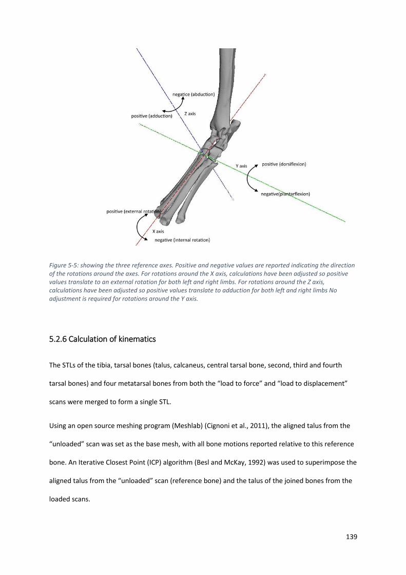
139

Figure 5-5: showing the three reference axes. Positive and negative values are reported indicating the direction of the rotations around the axes. For rotations around the X axis, calculations have been adjusted so positive values translate to an external rotation for both left and right limbs. For rotations around the Z axis, calculations have been adjusted so positive values translate to adduction for both left and right limbs No adjustment is required for rotations around the Y axis.

5.2.6 Calculation of kinematics

The STLs of the tibia, tarsal bones (talus, calcaneus, central tarsal bone, second, third and fourth

tarsal bones) and four metatarsal bones from both the “load to force” and “load to displacement”

scans were merged to form a single STL.

Using an open source meshing program (Meshlab) (Cignoni et al., 2011), the aligned talus from the

“unloaded” scan was set as the base mesh, with all bone motions reported relative to this reference

bone. An Iterative Closest Point (ICP) algorithm (Besl and McKay, 1992) was used to superimpose the

aligned talus from the “unloaded” scan (reference bone) and the talus of the joined bones from the

loaded scans.

140

Once the joined bones from the loaded scans were aligned, the position of the tibia, tarsal bones

(with the exception of the first tarsal bone) and 4 metatarsals were then recorded in both the “load

to force” and “load to displacement” positions. Briefly, the STL of each bone from the unloaded scan

were superimposed onto the joined bones using the ICP algorithm. This resulted in each individual

bone STL being recorded in an “unloaded” position, a “load to force” position and a “load to

displacement” position relative to the talus.

A 4X4 transformation matrix was obtained for the motion of each bone from the “unloaded” to the

“load to force” and “load to displacement” positions and decoded to yield the motion in 6 degrees of

freedom (3 translations along the X, Y and Z axes and 3 rotations around the X, Y and Z axes) using a

custom code (Mathematica, Wolfram, IL, USA) detailed in Appendix B

An overview of the sequential steps involved in calculating kinematics is shown in figure 5.6.

141

Figure 5-6: Shows the sequential steps involved in kinematic calculations. Following positioning in the limb loading jib (step 1), limbs undergo CT scanning (step 2) allowing the DICOM images to be exported to a computer where scans are segmented (step 3) based on Hounsfield units. From the segmented scans, 3 dimensional sterolithographic bone models are created (step 4) and aligned to anatomical reference axes (step 5). The reference bone of two scans are superimposed (step 6) allowing the motion of each bone from one scan to the next to be calculated (step 7)

142

5.2.7 Description of bone motion

As an alternative to reporting in 6 degrees of freedom, rigid body transformations can be reported

as a single summative rotation around a helical axis. This single rotation was termed total rotation.

The magnitude of rotation around and orientation of the helical axis was calculated for each bone

based upon previously published calculations (Panjabi, 1979; Spoor and Veldpaus, 1980; Woltring et

al., 1985) and processed using coding in commercially available software (Mathematica, Wolfram, IL,

USA). The orientation and position of the axis was reported as a point (x,y,z co-ordinates) and three

vectors. In order to calculate how well aligned the helical axes of two bones were, the angle

between these two axes in 3D space (alignment angle) was calculated using the following formula:

Alignment angle (AA) (degrees) = A cos ((x1 X x2)+(y1 X y2)+(z1 X z2)) X 180/

Equation 5.1: Calculation of the alignment angle

Where,

x1= x vector component of helical axis of bone 1

x2 = x vector component of helical axis of bone 2

y1= y vector component of helical axis of bone 1

y2 = y vector component of helical axis of bone 2

z1= z vector component of helical axis of bone 1

z2 = z vector component of helical axis of bone 2

143

5.2.8 Kinematics relative to the sagittal plane

To calculate the contribution each joint made to the overall motion in the sagittal plane, only

rotation around the Y axis was considered. The limb was divided into two kinematic chains; the

medial column, which comprised the talus, central, third tarsal bone and third metatarsal and the

lateral column, which comprised the calcaneus, fourth tarsal bone and fourth metatarsal bone. The

relative contribution of each joint in the chain to sagittal plane potation was compared between the

two loading patterns.

In order to compare the orientation of the helical axis of multiple bones in one analysis, the angle

between the helical axis and the y axis of our co-ordinate system was calculated for each bone. As

rotation around the y axis occurs in the sagittal plane, this angle represents the deviation in rotation

away from the sagittal plane. This angle was termed the sagittal deviation angle (SDA) and was

calculated using equation 5.2.

Sagittal deviation angle (degrees)= Acos (y vector component) X 180/

Equation 5.2: was used to calculate the sagittal deviation angle

144

5.2.9 Statistical analysis

All statistical analyses were performed using the commercially available statistical package Genstat

(VSNi, Hemel Hempstead, UK). Descriptive data was performed for translations and rotations about

the anatomically based axis, the magnitude of rotation around the helical axis and the orientation of

the helical axis in relation to the sagittal plane. A paired t-test was used to compare hock angles

between load to force and load to displacement. Similarly, a paired t-test was used to compare load

recorded on the foot plate for both loading positions. All data was checked for normality using the

Anderson-Darling test before further analysis. To compare the SDA, a general mixed linear model

was used to evaluate the effect of bone, cadaver (dog 1-5), side (left or right limb) and loading

pattern (load to force or load to displacement) on the SDA. Values of p<0.05 were considered

significant.

A general linear model was also used to evaluate the effect of cadaver and side on the magnitude of

rotation around the helical axis. As the magnitude would be expected to vary depending on load

condition, one model was created for each load condition. To identify if any kinematic coupling

existed, the magnitude of rotation for each pair was plotted using Excel (Microsoft, Redmond,

Washington, USA) to yield a correlation coefficient (R2) and kinematic coupling ratio (slope of the

trendline).

A paired t-test was used to compare the relative contribution of each joint in the chain to sagittal

plane rotation for both patterns of loading.

145

5.3 Results

5.3.1 Description of tarsal bone kinematics in 3 dimensions:

5.3.1.1 Six degrees of freedom descriptions

All bones demonstrated translation and rotation relative to the reference bone (talus). A summary of

these motions along and around each reference axis is provided for load to force (table 5.1) and load

to displacement (table 5.2).

Table 5-1: The mean motion of the tibia, tarsal bones and metatarsal bones following application of a standard (600N) load. The data is provided as a series of three translations and three rotations along and around the previously described reference axes. All motion is relative to the reference bone, the talus. From this table it is clear that there is motion about all three axes and not only about the sagittal plane. CTB = central tarsal bone, TB = tarsal bone, MT= metatarsal bone

x axis y axis z axis x axis y axis z axis

mean 19.98 1.66 10.47 0.72 -15.62 1.52

SD 5.13 1.66 1.69 1.08 2.01 0.77

mean 0.21 0.24 0.08 -1.37 1.13 -0.40

SD 0.13 0.07 0.08 0.80 0.72 0.25

mean 0.15 0.39 0.54 -1.35 2.18 -0.40

SD 0.09 0.13 0.21 0.64 1.01 0.26

mean 0.22 0.62 1.03 -1.50 2.55 -0.83

SD 0.13 0.19 0.42 0.59 1.17 0.19

mean 0.14 0.64 1.14 -0.89 3.25 -0.80

SD 0.09 0.19 0.43 0.63 1.19 0.26

mean 0.22 0.63 0.98 -0.89 3.74 -1.05

SD 0.10 0.19 0.40 0.70 1.57 0.76

mean 0.28 1.72 4.48 0.45 5.45 -1.37

SD 0.13 0.42 1.31 0.47 1.48 0.39

mean -0.17 1.71 5.30 0.55 5.94 -1.10

SD 0.10 0.45 1.60 0.66 1.60 0.41

mean -0.23 1.84 5.36 -1.47 6.13 -1.58

SD 0.11 0.47 1.70 1.30 1.63 0.47

mean 0.05 1.87 5.37 -1.39 6.08 -1.48

SD 0.10 0.50 1.66 1.45 1.54 0.46

MT III

MT IV

MT V

Calcaneus

CTB

Fourth TB

Third TB

Second TB

MT II

translation along (mm) rotation around (degrees)

Tibia

Load to force (600N)

146

Table 5-2: The mean motion of the tibia, tarsal bones and metatarsal bones following loading to a predetermined displacement (load to displacement). The data is provided as a series of three translations and three rotations along and around the previously described reference axes. All motion is relative to the reference bone, the talus. From this table it is clear that there is motion about all three axes and not only about the sagittal plane. CTB = central tarsal bone, TB = tarsal bone, MT= metatarsal bone

5.3.1.2 Description as a single rotation around helical axis

When expressed as total rotation around the helical axis, there were significant differences between

the magnitude of rotation for different bones but no significant effect of side (p=0.183 for load to

force, p=0.390 for load to displacement) or dog (p=0.093 for load to force, p=0.144 for load to

displacement).

For both load conditions the tibia showed the greatest total rotation and was significantly different

to all other bones. The was no difference in total rotation between the four metatarsal bones and

the second, third and fourth tarsal bone for each load condition (figure 5.7)

x axis y axis z axis x axis y axis z axis

mean 37.82 2.85 15.14 1.93 -28.60 3.14

SD 5.25 2.78 3.54 1.97 3.30 1.61

mean 0.42 0.40 0.14 -2.71 2.05 -0.76

SD 0.29 0.09 0.18 1.46 1.49 0.45

mean 0.22 0.80 1.03 -1.92 4.56 -1.18

SD 0.16 0.22 0.45 0.78 2.08 0.51

mean 0.35 1.14 1.85 -2.07 4.75 -1.51

SD 0.22 0.32 0.86 0.74 2.32 0.32

mean 0.15 1.22 2.13 -1.12 5.99 -1.72

SD 0.16 0.32 0.94 0.70 2.30 0.63

mean 0.32 1.20 1.91 -1.40 5.81 -0.98

SD 0.17 0.32 0.90 0.93 2.51 1.92

mean 0.09 2.92 8.84 1.83 10.84 -2.03

SD 0.33 0.71 2.92 1.15 3.12 0.64

mean -0.85 3.20 10.22 1.71 11.62 -2.10

SD 0.50 0.80 3.30 0.88 3.11 0.71

mean -0.90 3.43 10.00 -1.97 11.54 -3.11

SD 0.48 0.78 3.28 1.49 3.00 0.76

mean -0.32 3.47 9.78 -1.93 11.11 -3.01

SD 0.28 0.71 2.92 1.63 2.63 0.67

Tibia

Load to displacement

MT IV

MT V

CTB

Fourth TB

Third TB

Second TB

MT II

MT III

Calcaneus

translation along (mm) rotation around (degrees)

147

Figure 5-7: The total rotation of each bone around it’s own helical axis for both loading conditions. Each bone underwent greater rotation when loaded to displacement rather that to 600N of force. There was greatest motion at the talocrural joint, followed by the tarsometatarsal joint with the least motion observed between the tarsal bones themselves. CTB = central tarsal bone, Fourth = fourth tarsal bone, Third = third tarsal bone, Second = second tarsal bone, MT = metatarsal

The calcaneus and central tarsal bones showed no difference in total rotation compared to the

numbered tarsal bones, with the exception of the calcaneus, which rotated significantly less than the

second tarsal bone in the load to displacement scan.

The orientation of the helical axis of each bone was oblique to the reference co-ordinate axis was

located remotely to the bone itself in all cases other than the calcaneus (figures 5.8 and 5.9) The

vectors for each axis are available in Appendix C

0.00

5.00

10.00

15.00

20.00

25.00

30.00

35.00R

ota

tio

n a

rou

nd

hel

ical

axi

s (d

egre

es)

Bone

load to force

load to displacement

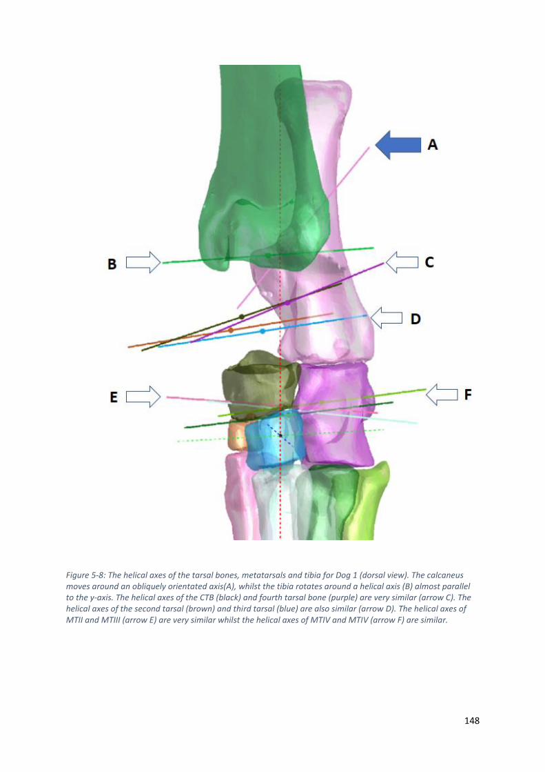
148

Figure 5-8: The helical axes of the tarsal bones, metatarsals and tibia for Dog 1 (dorsal view). The calcaneus moves around an obliquely orientated axis(A), whilst the tibia rotates around a helical axis (B) almost parallel to the y-axis. The helical axes of the CTB (black) and fourth tarsal bone (purple) are very similar (arrow C). The helical axes of the second tarsal (brown) and third tarsal (blue) are also similar (arrow D). The helical axes of MTII and MTIII (arrow E) are very similar whilst the helical axes of MTIV and MTIV (arrow F) are similar.

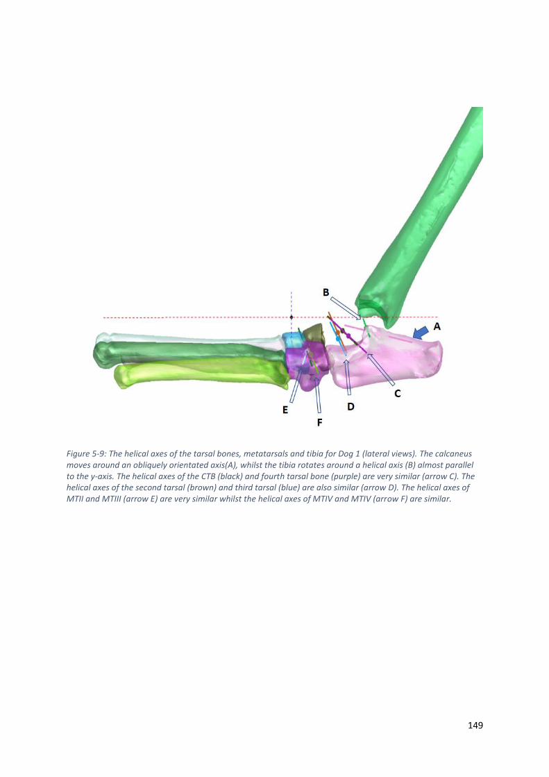
149

Figure 5-9: The helical axes of the tarsal bones, metatarsals and tibia for Dog 1 (lateral views). The calcaneus moves around an obliquely orientated axis(A), whilst the tibia rotates around a helical axis (B) almost parallel to the y-axis. The helical axes of the CTB (black) and fourth tarsal bone (purple) are very similar (arrow C). The helical axes of the second tarsal (brown) and third tarsal (blue) are also similar (arrow D). The helical axes of MTII and MTIII (arrow E) are very similar whilst the helical axes of MTIV and MTIV (arrow F) are similar.

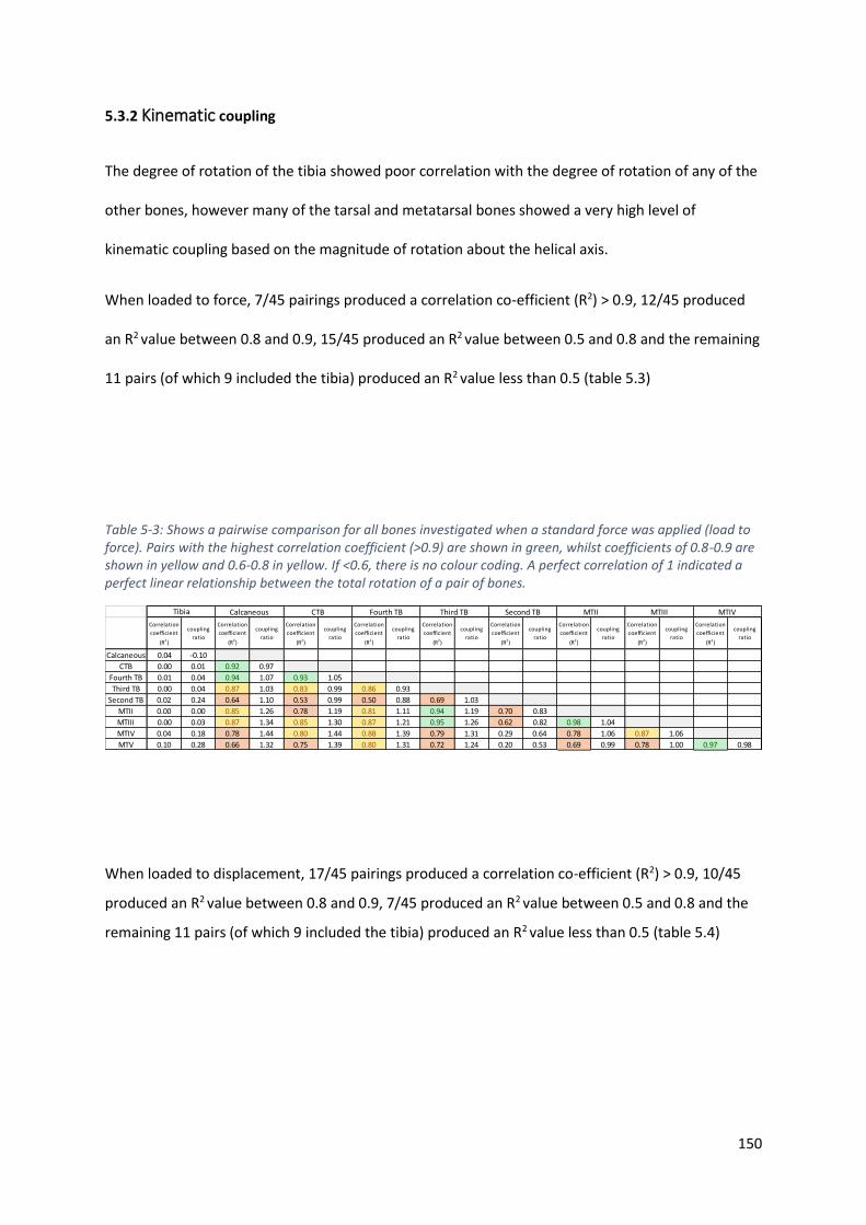
150

5.3.2 Kinematic coupling

The degree of rotation of the tibia showed poor correlation with the degree of rotation of any of the

other bones, however many of the tarsal and metatarsal bones showed a very high level of

kinematic coupling based on the magnitude of rotation about the helical axis.

When loaded to force, 7/45 pairings produced a correlation co-efficient (R2) > 0.9, 12/45 produced

an R2 value between 0.8 and 0.9, 15/45 produced an R2 value between 0.5 and 0.8 and the remaining

11 pairs (of which 9 included the tibia) produced an R2 value less than 0.5 (table 5.3)

Table 5-3: Shows a pairwise comparison for all bones investigated when a standard force was applied (load to force). Pairs with the highest correlation coefficient (>0.9) are shown in green, whilst coefficients of 0.8-0.9 are shown in yellow and 0.6-0.8 in yellow. If <0.6, there is no colour coding. A perfect correlation of 1 indicated a perfect linear relationship between the total rotation of a pair of bones.

When loaded to displacement, 17/45 pairings produced a correlation co-efficient (R2) > 0.9, 10/45

produced an R2 value between 0.8 and 0.9, 7/45 produced an R2 value between 0.5 and 0.8 and the

remaining 11 pairs (of which 9 included the tibia) produced an R2 value less than 0.5 (table 5.4)

Correlation

coefficient

(R2)

coupling

ratio

Correlation

coefficient

(R2)

coupling

ratio

Correlation

coefficient

(R2)

coupling

ratio

Correlation

coefficient

(R2)

coupling

ratio

Correlation

coefficient

(R2)

coupling

ratio

Correlation

coefficient

(R2)

coupling

ratio

Correlation

coefficient

(R2)

coupling

ratio

Correlation

coefficient

(R2)

coupling

ratio

Correlation

coefficient

(R2)

coupling

ratio

Calcaneous 0.04 -0.10

CTB 0.00 0.01 0.92 0.97

Fourth TB 0.01 0.04 0.94 1.07 0.93 1.05

Third TB 0.00 0.04 0.87 1.03 0.83 0.99 0.86 0.93

Second TB 0.02 0.24 0.64 1.10 0.53 0.99 0.50 0.88 0.69 1.03

MTII 0.00 0.00 0.85 1.26 0.78 1.19 0.81 1.11 0.94 1.19 0.70 0.83

MTIII 0.00 0.03 0.87 1.34 0.85 1.30 0.87 1.21 0.95 1.26 0.62 0.82 0.98 1.04

MTIV 0.04 0.18 0.78 1.44 0.80 1.44 0.88 1.39 0.79 1.31 0.29 0.64 0.78 1.06 0.87 1.06

MTV 0.10 0.28 0.66 1.32 0.75 1.39 0.80 1.31 0.72 1.24 0.20 0.53 0.69 0.99 0.78 1.00 0.97 0.98

Tibia Calcaneous CTB Fourth TB Third TB Second TB MTIVMTIIIMTII

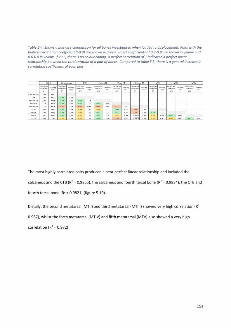
151

Table 5-4: Shows a pairwise comparison for all bones investigated when loaded to displacement. Pairs with the highest correlation coefficient (>0.9) are shown in green, whilst coefficients of 0.8-0.9 are shown in yellow and 0.6-0.8 in yellow. If <0.6, there is no colour coding. A perfect correlation of 1 indicated a perfect linear relationship between the total rotation of a pair of bones. Compared to table 5.3, there is a general increase in correlation coefficients of each pair

The most highly correlated pairs produced a near perfect linear relationship and included the

calcaneus and the CTB (R2 = 0.9855), the calcaneus and fourth tarsal bone (R2 = 0.9834), the CTB and

fourth tarsal bone (R2 = 0.9821) (figure 5.10).

Distally, the second metatarsal (MTII) and third metatarsal (MTIII) showed very high correlation (R2 =

0.987), whilst the forth metatarsal (MTIV) and fifth metatarsal (MTV) also showed a very high

correlation (R2 = 0.972)

Correlation

coefficient

(R2)

coupling

ratio

Correlation

coefficient

(R2)

coupling

ratio

Correlation

coefficient

(R2)

coupling

ratio

Correlation

coefficient

(R2)

coupling

ratio

Correlation

coefficient

(R2)

coupling

ratio

Correlation

coefficient

(R2)

coupling

ratio

Correlation

coefficient

(R2)

coupling

ratio

Correlation

coefficient

(R2)

coupling

ratio

Correlation

coefficient

(R2)

coupling

ratio

Calcaneous 0.07 -0.17

CTB 0.09 -0.20 0.99 1.06

Fourth TB 0.06 -0.18 0.98 1.15 0.98 1.08

Third TB 0.13 -0.26 0.97 1.15 0.97 1.07 0.95 0.98

Second TB 0.13 -0.28 0.70 1.05 0.71 0.99 0.63 0.85 0.71 0.91

MTII 0.02 -0.12 0.91 1.43 0.85 1.30 0.89 1.21 0.90 1.22 0.66 0.97

MTIII 0.02 -0.13 0.92 1.44 0.88 1.32 0.91 1.23 0.92 1.24 0.63 0.96 0.99 1.00

MTIV 0.01 -0.10 0.91 1.42 0.88 1.31 0.93 1.24 0.88 1.20 0.4462 0.80 0.89 0.94 0.92 0.95

MTV 0.00 0.00 0.85 1.23 0.84 1.14 0.90 1.09 0.79 1.02 0.3702 0.65 0.81 0.80 0.85 0.82 0.97 0.88

Tibia Calcaneous CTB Fourth TB Third TB Second TB MTII MTIII MTIV

152

Figure 5-10: plotting magnitude of rotation of a kinematic pair to derive a correlation coefficient and coupling ratio. CTB and calcaneus (top), Fourth tarsal and calcaneus (middle) and Fourth tarsal and CTB (bottom) all showed very high levels of kinematic coupling

y = 1.059x + 1.3558R² = 0.9855

0

1

2

3

4

5

6

7

8

9

10

0 2 4 6 8

Ro

tati

on

of

CTB

(d

egre

es)

Rotation of calcaneus (degrees)

y = 1.1522x + 1.3398R² = 0.9834

0

1

2

3

4

5

6

7

8

9

10

0 2 4 6 8

Ro

tati

on

of

fou

rth

tar

sal b

on

e (d

egre

ees)

Rotation of calcaneus (degrees)

y = 1.0794x - 0.0908R² = 0.9821

0

2

4

6

8

10

0 1 2 3 4 5 6 7 8 9 10

Ro

tati

on

of

the

fou

rth

tar

sal

bo

ne

(deg

rees

)

Rotation of the CTB (degrees)

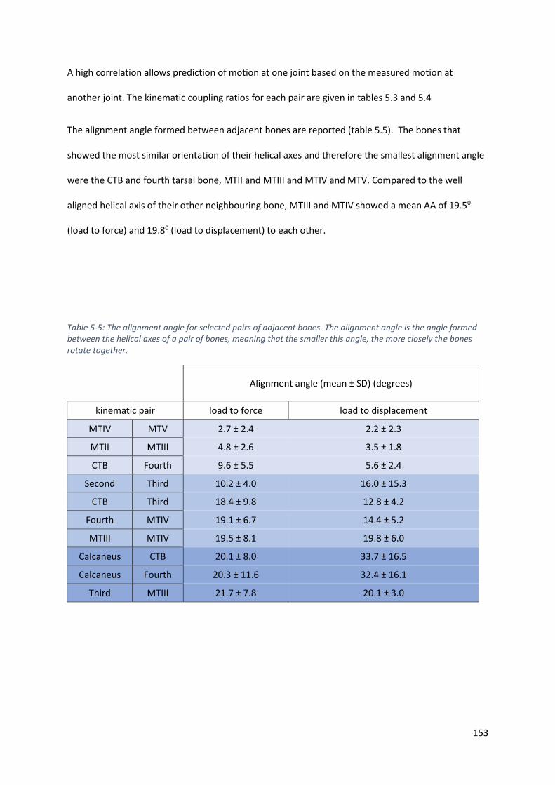
153

A high correlation allows prediction of motion at one joint based on the measured motion at

another joint. The kinematic coupling ratios for each pair are given in tables 5.3 and 5.4

The alignment angle formed between adjacent bones are reported (table 5.5). The bones that

showed the most similar orientation of their helical axes and therefore the smallest alignment angle

were the CTB and fourth tarsal bone, MTII and MTIII and MTIV and MTV. Compared to the well

aligned helical axis of their other neighbouring bone, MTIII and MTIV showed a mean AA of 19.50

(load to force) and 19.80 (load to displacement) to each other.

Table 5-5: The alignment angle for selected pairs of adjacent bones. The alignment angle is the angle formed between the helical axes of a pair of bones, meaning that the smaller this angle, the more closely the bones rotate together.

Alignment angle (mean ± SD) (degrees)

kinematic pair load to force load to displacement

MTIV MTV 2.7 ± 2.4 2.2 ± 2.3

MTII MTIII 4.8 ± 2.6 3.5 ± 1.8

CTB Fourth 9.6 ± 5.5 5.6 ± 2.4

Second Third 10.2 ± 4.0 16.0 ± 15.3

CTB Third 18.4 ± 9.8 12.8 ± 4.2

Fourth MTIV 19.1 ± 6.7 14.4 ± 5.2

MTIII MTIV 19.5 ± 8.1 19.8 ± 6.0

Calcaneus CTB 20.1 ± 8.0 33.7 ± 16.5

Calcaneus Fourth 20.3 ± 11.6 32.4 ± 16.1

Third MTIII 21.7 ± 7.8 20.1 ± 3.0

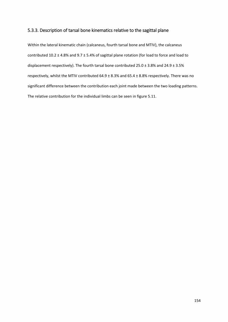
154

5.3.3. Description of tarsal bone kinematics relative to the sagittal plane

Within the lateral kinematic chain (calcaneus, fourth tarsal bone and MTIV), the calcaneus

contributed 10.2 ± 4.8% and 9.7 ± 5.4% of sagittal plane rotation (for load to force and load to

displacement respectively). The fourth tarsal bone contributed 25.0 ± 3.8% and 24.9 ± 3.5%

respectively, whilst the MTIV contributed 64.9 ± 8.3% and 65.4 ± 8.8% respectively. There was no

significant difference between the contribution each joint made between the two loading patterns.

The relative contribution for the individual limbs can be seen in figure 5.11.

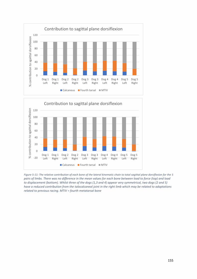
155

Figure 5-11: The relative contribution of each bone of the lateral kinematic chain to total sagittal plane dorsiflexion for the 5

pairs of limbs. There was no difference in the mean values for each bone between load to force (top) and load to displacement (bottom). Whilst three of the dogs (1,3 and 4) appear very symmetrical, two dogs (2 and 5) have a reduced contribution from the talocalcaneal joint in the right limb which may be related to adaptations related to previous racing. MTIV = fourth metatarsal bone

0

20

40

60

80

100

120

Dog 1Left

Dog 1Right

Dog 2Left

Dog 2Right

Dog 3Left

Dog 3Right

Dog 4Left

Dog 4Right

Dog 5Left

Dog 5Right

% c

on

trib

uti

on

to

sga

itta

l do

rsif

lexi

on

Contribution to sagittal plane dorsiflexion

Calcaneus Fourth tarsal MTIV

-20

0

20

40

60

80

100

120

Dog 1Left

Dog 1Right

Dog 2Left

Dog 2Right

Dog 3Left

Dog 3Right

Dog 4Left

Dog 4Right

Dog 5Left

Dog 5Right%

co

ntr

ibu

tio

n t

o s

gait

tal d

ors

ifle

xio

n

Contribution to sagittal plane dorsiflexion

Calcaneus Fourth tarsal MTIV

156

For the medial chain (CTB, third tarsal bone and MTIII) the CTB contributed 18.2 ± 4.9% and 19.8 ±

3.2% (for load to force and load to displacement respectively). The third tarsal bone contributed 28.3

± 2.5% and 26.6 ± 1.9% respectively, whilst the MTIII contributed 53.5 ± 5.7% and 53.5 ± 5.0%

respectively. There was no significant difference between the relative contributions of each bone at

the two patterns of loading (figure 5.12)

Figure 5-12: the relative contribution of each bone of the medial kinematic chain to total sagittal plane dorsiflexion for the 5 pairs of limbs. There was no difference in the mean values for each bone between load to force (top) and load to displacement (bottom). CTB = central tarsal bone, MTIII = third metatarsal bone.

0

20

40

60

80

100

120

Dog 1Left

Dog 1Right

Dog 2Left

Dog 2Right

Dog 3Left

Dog 3Right

Dog 4Left

Dog 4Right

Dog 5Left

Dog 5Right

% c

on

trib

uti

on

to

sga

itta

l do

rsif

lexi

on

Contribution to sagittal plane dorsiflexion

CTB Third tarsal MTIII

0

20

40

60

80

100

120

Dog 1Left

Dog 1Right

Dog 2Left

Dog 2Right

Dog 3Left

Dog 3Right

Dog 4Left

Dog 4Right

Dog 5Left

Dog 5Right%

co

ntr

ibu

tio

n t

o s

gait

tal d

ors

ifle

xio

n

Contribution to sagittal plane dorsiflexion

CTB Third tarsal MTIII

157

There was no significant effect of dog (p=0.283), side (p=0.812) or degree of loading (p=0.743) on

orientation of the helical axis relative to the sagittal plane (SDA) for each bone, suggesting that the

helical axis is well preserved between individuals and symmetrical within individuals. The orientation

of the axis also remained constant at both positions measured in this study. There was significant

variability when comparing the SDA of the individual tarsal bones, metatarsal bones and tibia (figure

5.13) The calcaneus showed the greatest SDA (mean 57.50 ± SD 14.30) and was significantly different

to the helical axis of all other bones except the CTB (32.90 ± 9.30) fourth tarsal bones (34.50 ± 8.40).

The SDA of the tibia showed the least deviation from motion from the sagittal plane and was

significantly different from all other bones.

The bones with the smallest SDA, the tibia and metatarsals, also demonstrated the greatest

magnitude of rotation, whilst the bone with the largest SDA showed the least total rotation.

158

Figure 5-13: The sagittal plane deviation angle (SDA) for each of the bones. This angle is measured between the helical axis and the y-axis. As rotation around the y-axis occurs in the sagittal plane, the SDA represents deviation in the rotation of the bone away from the sagittal plane. Error bars represent one SD. From this graph it can be seen that the high motion talocrural joint acts primarily in the sagittal plane, whilst many of the tarsal bones rotate around an oblique helical axis that

is not closely aligned with sagittal plane rotation. . CTB = central tarsal bone, Fourth = fourth tarsal bone, Third = third tarsal bone, Second = second tarsal bone, MT = metatarsal

0.00

10.00

20.00

30.00

40.00

50.00

60.00

70.00

80.00

90.00

Tibia Calcaneus CTB Fourth Third Second MTII MTIII MTIV MTV

SDA

(d

egre

es)

Bone

Sagittal Deviation Angle for tarsal and metatarasal bones

159

5.4 Discussion

The complex and highly coupled kinematics of the canine tarsal bones have been characterised using

a newly validated limb loading jig and accurate, non-invasive measurement technique. The findings

of this experiment support the first hypothesis that individual tarsal bone motion occurs out of the

sagittal plane. The data also confirms that dorsiflexion of the pes occurs during loading of the hind

limb, supporting our second hypothesis, and this motion is facilitated by a highly coupled kinematic

chain that extends from the talus to the metatarsal bones. The identification of rigid functional units

within the pes, supports the third hypothesis that some bones move almost in perfect unison and

may allow development of more simplified models of the canine pes.

5.4.1 Contribution of the tarsal joints to hock flexion

Motion at all tarsal and metatarsal joints was identified, meaning each articulation contributed to

the overall motion of the distal limb. The talocrural joint has been reported to contribute 90% of the

overall motion in the hock (Carmichael and Marshall, 2013) and although the results of this

experiment found this joint contributed the majority of sagittal plane dorsiflexion, the tarsal and

tarsometatarsal joints contributed a mean of 27.6% and 28.9% of total sagittal plane dorsiflexion

when loaded to force and displacement respectively. This translated into a mean of 11.40 and 22.20

degrees of sagittal plane dorsiflexion when loaded to force and displacement respectively. If the pes

is considered as a rigid body, and the hock modelled as a simple gingylmus, as in many kinematic

studies (Fu et al., 2010; Headrick et al., 2014b; Hottinger et al., 1996), inaccuracies will result. Small

but potentially significant motions at the intertarsal and tarsometatarsal joints will be overlooked,

whilst movement will be incorrectly attributed to adjacent joints, and may impact upon derived

calculations such as power and work.

160

The contribution of intertarsal and tarsometatarsal joints to dorsiflexion of the pes in any species

remains widely unknown. In the running camel, approximately 17 degrees of dorsiflexion was

attributed to dorsiflexion at the proximal intertarsal and tarsometatarsal joints (Alexander et al.,

1982) and this motion was a vital component of the energy storage mechanism in this species,

allowing increased energy storage in flexor tendons. In the greyhound, the gastrocnemius,

superficial and deep digital flexor muscles all demonstrate a high tendon length change: muscle

fascicle length, indicating a reliance on passive length change (tendon elongation) rather than active

muscle shortening for function (Williams et al., 2009). It may be suggested that dorsiflexion of the

canine pes allows greater elongation and hence energy storage within the digital flexor tendons as

seen in other species (Alexander et al., 1982; Alexander, 1984; Vereecke and Aerts, 2008).

Dorsiflexion of the pes may also allow storage of elastic energy within the passive structures of the

foot. Up to 17% of the elastic energy storage in the human leg is believed to be stored within the

plantar aponeurosis, spring ligament and long and short plantar ligaments (Ker et al., 1987).

5.4.2 Patterns of tarsal bone kinematics

The orientation of the helical axis of each bone was identified and the magnitude of rotation was

reported, revealing a consistent pattern of motion between all dogs. The helical axis represents the

3D axis around which a bone rotates and is commonly used in kinematic investigations (Beimers et

al., 2008; Kirby, 2000; Sennwald et al., 1993). Sennwald et al. (1993) suggested that complex

motions may not be completely characterized by use of a single helical axis. For example, if a bone

translates then subsequently rotates, it would be best characterized by identifying one helical axis

that describes the initial translation and another that characterizes the latter rotation. Results of this

chapter revealed that the helical axes did not show significant differences in position between the

two loading patterns suggesting that the canine tarsal bones continue to rotate around a very similar

helical axis throughout their motion. With the exception of the calcaneus, the position of the helical

axis of each bone that was investigated was remote to the bone itself, implying a gliding pattern of

161

motion. This can result in significant movement through translation despite only limited rotation

(Sennwald et al., 1993).

The tarsal and tarsometatarsal joints show high levels of kinematic coupling, defined as

intersegment co-ordination (Wilken et al., 2011) resulting in a distinct pattern of movement that

allows the pes to function as a unit. The orientation of the helical axes of the tarsal bones all run

from a proximal, lateral and caudal position in a distal, medial and cranial direction.

5.4.2.1 The calcaneus

The helical axis of the calcaneus shows the greatest obliquity, producing more internal rotation than

dorsiflexion during loading. As the only tarsal bone with the helical axis located within the bone

itself, the calcaneus undergoes little translation. The orientation and position of this axis is

consistent with the oblique, compromise helical axis reported in man, where foot inversion and

eversion plays an important role in foot function (Beimers et al., 2008) and in a wide variety of other

species (Lewis, 1980) suggesting the helical axis of the calcaneus is well preserved across species

despite great differences in the pattern of locomotion.

5.4.2.2 The bones of the mid foot

The helical axes around which the CTB and fourth tarsal bone rotate are well aligned, with an

alignment angle of less than 10 degrees. Like the calcaneus, their oblique axes results in dorsiflexion

coupled with internal rotation, however, due to the decreased obliquity of the helical axis compared

to the calcaneus, both the CTB and fourth tarsal bone show greater a greater dorsiflexion

component than internal rotation component. The magnitude of rotation of these bones about their

helical axis are highly kinematically coupled to each other and to that of the calcaneus. Despite being

spanned by the fourth tarsal bone, motion was consistently identified at the centro-distal joint.

Rotating around a similar oblique helical axis, the second and third tarsal bones also demonstrate

internal rotation coupled with dorsiflexion. However, as the SDA is less than for the calcaneus, CTB

162

and fourth tarsal bone, the dorsiflexion component of rotation is the major component with

significantly less internal rotation. These bones may play a major role in facilitating the differing, but

complementary motions of the metatarsal bones as discussed below.

5.4.2.3 Metatarsal bones

There was high kinematic coupling of the magnitude of rotation of MTIV and MTV and these bones

displayed well aligned helical axes. Similar to the other tarsal bones, dorsiflexion of these joints was

coupled with slight internal rotation. MTII and MTIII demonstrated tight coupling and well aligned

helical axes, however, these bones displayed an external rotation coupled with dorsiflexion. This

change in direction of rotation on either side of the midline of the pes results in a flattening of the

natural arc of the metatarsals in the transverse plane. This may act to further increase elastic storage

in the foot, being returned during the take-off phase of gait. Additionally, the internal rotation of the

lateral metatarsals and external rotation of the medial metatarsals may facilitate equalization of

pressure on all digital foot pads despite an internal rotation of the more proximal aspect of the pes.

Apart from the common calcaneal tendon insertion, there are no muscular attachments of

significance on the tarsal bones that are active during the stance phase (Evans et al., 2012; Goslow et

al., 1981) and therefore the motion of these bones is the result of the direct force from adjacent

bones and the limiting effects of ligaments and the joint capsule. A similar situation is reported in

the human wrist, where the bones of the proximal carpal row will self-align as they move towards

extremes of motion (Sennwald et al., 1993). The increased kinematic coupling seen at higher loads in

this experiment, support the fact that bones of the tarsus self-align during loading, taking position as

dictated by adjacent joint surfaces and limited by the vast array of ligaments that attach to the tarsal

and adjacent bones (Aron and Purinton, 1985a; Evans et al., 2012; Gorse et al., 1990). Ligaments

have been shown to possess non-linear viscoelastic properties (Attarian et al., 1985; Crary et al.,

2003; Funk et al., 2000), becoming stiffer as the load increases and further restricting bone motion

163

at the limits of motion. The increased coupling demonstrated at higher loads in our study is an

example of the effect of this biomechanical property. However, as ligaments act as elastic tissues

within their functional range, it is possible that the well-developed plantar ligaments in the canine

foot may also contribute to energy storage as the pes dorsiflexes.

Divergence of the helical axis of adjacent bones has been proposed as one mechanism that may

“lock” bones into position at extremes of motion, providing a more rigid level off which to propel.

This has been described in the human mid-foot (Blackwood et al., 2005) (Okita et al., 2014).

However, it is observed that there is no obvious divergence amongst the helical axes of the tarsal

bones but rather a gradual transition in obliquity from the most oblique axis of the calcaneus, to the

most distal tarsometatarsal joints, which show very little divergence from sagittal plane dorsiflexion.

This anatomical arrangement makes a locking mechanism unlikely in the dog. Furthermore, the

positioning of the helical axes remote from the bone creates a gliding motion at the flat or

spheroidal articular surfaces with no obvious end point created by the bone shape alone. This

arrangement would be biomechanically advantageous to a limb that acts as a biological spring,

limiting motion by the elastic potential of ligaments and tendons rather than compressive forces of

adjacent bones which would produce a more abrupt end-point.

During take-off from the stance phase, the pes undergoes an external rotation coupled with

plantarflexion (foot inversion), which has been demonstrated in the human foot after heel lift (Kirby,

2000). It has been proposed that this external rotation brings the fourth tarsal bone into a more

plantar position, whilst the CTB takes a more lateral and dorsal position, producing a more vertical

alignment of the proximal intertarsal joint which provides a more rigid lever from which to push off.

There are obvious differences between the human and canine foot during the early stance phase,

where the plantigrade human foot undergoes a heel strike followed by a flat foot phase in contrast

to the dog which remains digitigrade. However, the pattern of motion after heel lift in the human is

164

likely to be similar to the take-off phase in the canine foot and our findings of coupled external

rotation with plantarflexion are consistent to that of human kinematic foot studies.

5.4.3 A simplified model of the canine foot

By quantifying the motion of each tarsal bone in a series of canine cadavers, bones that consistently

move a similar magnitude around a similarly orientated axis were identified. Depending on the

aspect of motion being studied, small movements between bones may be significant, whilst in other

situations, the pes may be simplified into a smaller number of functional units. A number of bones

that were investigated as part of this experiment may be considered as functional units, therefore

simplifying future kinematic studies, particularly those involving instrumentation of bones. The

medial two metatarsal bones (MTII and MTIII) showed a very similar magnitude of rotation around

their helical axes, which were also aligned in a similar orientation in 3D space. These two bones were

the only bones to undergo external rotation during dorsiflexion and were also highly kinematically

coupled. Therefore, it may be suggested that these two bones could be considered as a rigid

functional unit. Similarly, the lateral two metatarsals (MTIV and MTV) also showed a very similar

magnitude of rotation about closely orientated axes and could be considered as a rigid functional

unit. The medial and lateral metatarsals provide easily identifiable and palpable landmarks that can

be visualized throughout gait if markers are used. The CTB and fourth tarsal bones can also be

considered to form a mid-foot rigid function unit in the canine tarsus as they meet the same criteria

as the metatarsal units. Despite a high kinematic coupling with the calcaneus, the CTB and fourth

tarsal bones rotate about a very different helical axis and so although these three bones work in

synchrony, they cannot be considered to form one rigid functional unit. Kinematic coupling between

the tibia and any of the tarsal bones was not identified. This may be because no coupling exists or

because our limb loading jig did not replicate the forward motion of the tibia as it moves over the

planted foot during the gait cycle.

165

A simplified model of the tarsal and metatarsal bones may allow motion to be attributed more

appropriately to the talocrural joint and the individual intertarsal and tarsometatarsal joints. This

may be particularly important in in vivo studies, where identification of all individual tarsal bones

may be challenging. The high kinematic coupling between the tarsal bones mean that

instrumentation of each bone may not be required and that if motion between two adjacent or

potentially non-adjacent bones can be accurately measured in a given plane, then the 3D motion at

other joints may be able to be accurately derived.

5.4.4 Study limitations

The major limitation with any cadaveric kinematic study is the need to accurately replicate the

forces that result in bone displacement. This has been achieved previously with the use of motors

attached to tendons in walking models. One of the key features of these jigs is that they preserve

the natural insertion of the tendon onto bone, the enthesis. This ensures the tensile force on the

bone is accurately reproduced. The experimental design used in this chapter preserved both the

gastrocnemius muscle and superficial digital flexor muscle as they spanned between the caudodistal

aspect of the femur and calcaneus. The gastrocnemius muscle, in particular, is covered in a strong

fascial sheath and the short pennate fibres are infiltrated throughout with connective tissue. During

loading, the simultaneous stifle and hock angles recorded in a galloping dog were able to be

replicated. This required some lengthening of the gastrocnemius muscle, which occurred in our

specimens and has also been recorded in vivo in the galloping dog (Goslow et al., 1981).

Furthermore, the ground reaction force that results from tension in the common calcaneal tendon

was similar between our specimens and GRFs measured in galloping dogs for a given hock angle.

Therefore, it is suggested that the jig used in this experiment can accurately replicate the tensile

force in the common calcaneal tendon in a cadaveric specimen.

166

The only other muscular insertions on the canine tarsal bones belong to flexors of the hock (Cranial

tibial muscle, fibularis longus muscle and fibularis brevis muscle), which are not active during the

initial stance phase and very small muscles, such as the quadratus plantae, which are generally

considered insignificant. Therefore, this experimental design replicates the relevant muscle forces

during the stance phase of gait. It must also be recognised that although there may be no other

muscular insertions, there are a number of tendons that run across the tarsal bones and these may

also influence kinematics. From this experiment, which did not replicate all muscular forces, we

cannot speculate on the effect that these tendons may have had on tarsal kinematics.

There are intrinsic muscles of the pes that may influence motion but these are generally considered

as digital flexors. As no attempts were made to replicate natural forces acting on the phalangeal

bones, the motion of these bones was not recorded.

In this experiment, only one breed, the greyhound, was investigated as this breed is of consistent

size and conformation and would minimize inter-specimen variation. Care must be taken when

extrapolation these finding to other breeds, which may have differences in the degree of motion and

direction of motion of each bone. Greyhounds have undergone intense selection and display

significant anatomical and functional differences when compared to other breeds (Williams et al.,

2008). They are highly adapted for high speed locomotion and demonstrate a different distribution

of power across the hind limb joints when compared to Labradors (Colborne et al., 2005). Their

narrow and slender feet are another adaptation for speed, resulting in a different pattern of force

distribution through the pads when compared to a Labrador Retriever (Besancon et al., 2004). Based

upon palpation of dogs of several different breeds, it is possible that other breeds may show greater

tarsal movement and future studies comparing breeds would be of great value. The greyhounds

used in this study have an unknown history but it is likely that they have been involved with training

and racing. Always racing counter-clockwise around an oval track leads to asymmetrical tarsal and

metatarsal bone adaptive remodelling (Johnson et al., 2000; Johnson et al., 2001) and this fact may

167

influence tarsal bone kinematics. A paired limb design was chosen to address this potential

confounding factor and side was included as a factor in our statistical model, which demonstrated

there was no significant effect of side on tarsal bone kinematics.

The results reported in this chapter must also be interpreted in the light of the earlier experiments

of chapter 3, which detail the accuracy of the measurement technique employed. It is possible that

some of the small motions detected, particularly in the x axis, may reflect “noise” or alternatively

very small potions associated with compression of articular cartilage.

168

5.5 Conclusions

Far from a rigid structure, the canine pes undergoes elastic deformation during weight bearing,

facilitating storage of energy as elastic strain and increasing the efficiency of locomotion. The

dorsiflexion of the pes involves highly coupled motions at adjacent and non-adjacent joints, with

each bone rotating about its unique helical axis. The most rotation occurs in joints where rotation is

more closely aligned with the sagittal plane of the foot, whilst the most highly constrained joints

demonstrate more oblique helical axes. The pes shows abduction and internal rotation during

dorsiflexion and adduction and external rotation during plantarflexion at take-off.

169

Chapter 6 : The plantar ligament: Role in

tarsal bone kinematics and force

transmission

170

6.1 Introduction

Proximal intertarsal luxation or subluxation of the canine tarsus results in a debilitating lameness

that will not resolve without surgical intervention (Campbell et al., 1976; Dieterich, 1974; Lawson,

1960). There are numerous reports of this condition (Allen et al., 1993; Barnes et al., 2013; Dieterich,

1974; Fettig et al., 2002; Lawson, 1960; Wilke et al., 2000) with some reporting that proximal

intertarsal luxation is the most commonly encountered lesion of the canine hock in their hospital

population, accounting for 35% of all hock lesions (Campbell et al., 1976). Damage or degeneration

of the plantar ligamentous support has been suggested as the underlying cause of proximal

intertarsal subluxation (Allen et al., 1993; Barnes et al., 2013; Campbell et al., 1976; Lawson, 1960),

however, further characterisation of which components of the complex plantar ligamentous support

are damaged to permit subluxation have not been reported (Barnes et al., 2013).

The tarsal ligaments connect all aspects of the tarsal bones but are most significant on the plantar

surface, resisting the dorsiflexion of the pes during weight bearing (Carmichael and Marshall, 2013).

The canine plantar ligament has been previously described as having three components (Barnes et

al., 2013; Evans et al., 2012). The most lateral component, termed the calcaneoquartal ligament

(Evans et al., 2012) is also known as the lateral plantar ligament (Carmichael and Marshall, 2013) and

forms a small but distinct band running from the plantarolateral aspect of the tuber calcanei to the

head of the fifth metatarsal and fourth tarsal bone. The long plantar ligament, also termed the

middle plantar ligament (Carmichael and Marshall, 2013) is significantly larger, and its parallel fibres

run from the plantar aspect of the distal calcaneus to the thick fibrocartilage of the tarsometataral

joint capsule, inserting on the plantar process of the fourth tarsal bone as they pass over it (Evans et

al., 2012). The most medial component of the plantar ligament is known as the calcaneocentral

ligament or medial plantar ligament (Carmichael and Marshall, 2013), which runs from the plantar

aspect of the sustentaculum tali to the plantar process of the central tarsal bone. The fibres continue

171

distally as the plantar centrodistal ligament, which also inserts upon the thick fibrocartilage of the

tarsometatarsal joint capsule (Campbell et al., 1976; Evans et al., 2012).

The work of the previous chapter in this thesis demonstrates that motion occurs between all tarsal

bones during loading, making important contributions to overall hock flexion. However, it remains

unclear what role the various components of the plantar ligament play in tarsal bone kinematics in

the normal limb and what components of the plantar ligaments must be damaged to allow proximal

intertarsal subluxation.

Stability across the proximal intertarsal joint is essential for allowing the pes to act as the rigid beam

of a lever, rotating about the trochlea of the talus, which acts as the fulcrum (Pratt, 1935) (Ker et al.,

1987). The tensile force exerted on the tuber calcanei by the common calcaneal tendon allows

generation of a ground reaction force at the paw when the integrity of the pes is maintained.

Conversely, when the integrity of the pes is lost, as in proximal intertarsal subluxation, force

transmission through the pes, which permits generation of a ground reaction force, is also

presumably reduced (figure 6.1).

Figure 6-1: Left: the intact pes acts as a lever arm in the distal limb, rotating around a fulcrum (the trochlea of the talus). A tensile force (A) exerted by the common calcaneal tendon, creates a ground reaction force (B), which was measured using pressure sensitive film. Right: if the integrity of the pes is lost as seen in proximal intertarsal luxations, then the tensile force (A) cannot generate a ground reaction force.

172

To determine the role each component of the plantar ligament plays in tarsal bone kinematics and

force transmission through the pes, serial transection of the plantar ligament was performed in

cadaveric specimens and bone motions measured using CT based kinematic measurements. The aim

of this study was to characterise tarsal bone kinematics and measure force transmission in the intact

canine cadaver foot, following transection of the medial aspect of the plantar ligament

(calcaneocentral ligament), the lateral aspect of the plantar ligament (long plantar ligament) and

following transection of both of the major components of the plantar ligament. The null hypothesis

was that partial or full transection of the plantar ligament would produce no difference in tarsal

bone kinematics and force transmission through the pes when compared to the intact canine pes.

The calcaneoquartal ligament has been previously described as the third component of the plantar

ligament, but was not included in the transection model due to its lateral position that is unlikely

resist dorsiflexion of the pes and its relatively insignificant size compared to the other components

of the plantar ligament. Furthermore, despite being described as a component of the planter

ligament, this thin band actually represent an entirely tendinous muscle (m. abductor digiti V).

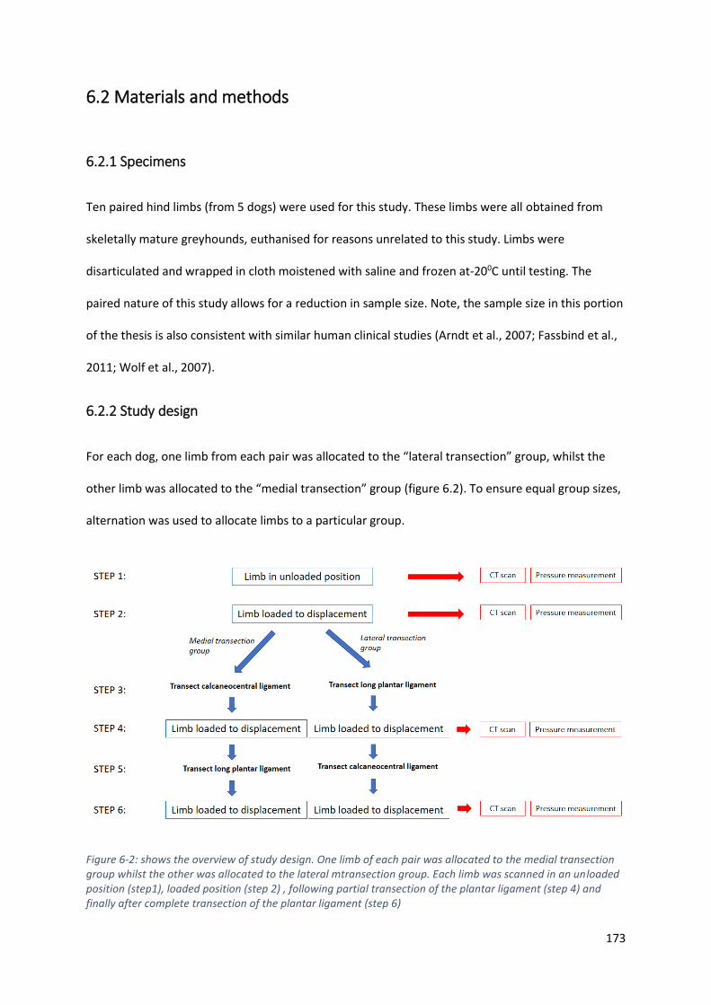
173

6.2 Materials and methods

6.2.1 Specimens

Ten paired hind limbs (from 5 dogs) were used for this study. These limbs were all obtained from

skeletally mature greyhounds, euthanised for reasons unrelated to this study. Limbs were

disarticulated and wrapped in cloth moistened with saline and frozen at-200C until testing. The

paired nature of this study allows for a reduction in sample size. Note, the sample size in this portion

of the thesis is also consistent with similar human clinical studies (Arndt et al., 2007; Fassbind et al.,

2011; Wolf et al., 2007).

6.2.2 Study design

For each dog, one limb from each pair was allocated to the “lateral transection” group, whilst the

other limb was allocated to the “medial transection” group (figure 6.2). To ensure equal group sizes,

alternation was used to allocate limbs to a particular group.

Figure 6-2: shows the overview of study design. One limb of each pair was allocated to the medial transection group whilst the other was allocated to the lateral mtransection group. Each limb was scanned in an unloaded position (step1), loaded position (step 2) , following partial transection of the plantar ligament (step 4) and finally after complete transection of the plantar ligament (step 6)

174

6.2.3 Limb loading

All limbs were prepared as previously described and loaded into a custom loading jig (described in

chapter 4). Prior to testing, the samples were thawed to room temperature and remained hydarated

with saline to avoid any drying artefact. The stifle and tarsal joints were manually flexed and

extended and preconditioned in the jig to a force of 600N, measured on the pressure sensitive film

(Film code 5076-350. Tekscan, South Boston, MA, USA ) positioned under the paw and cycled for five

repetitions (as described in Chapter 5). This force represents the approximate ground reaction force

measured from galloping dogs of similar size dogs, recorded from in vivo kinetic investigations

(Walter and Carrier, 2007) and has been discussed in the previous chapters of this thesis.

6.2.4 Computed tomographic scanning

All limbs were scanned using a 16-slice helical CT scanner (Philips Brilliance 16-slice CT scanner) with

scanning parameters (120KVP, 117 mA, slice thickness 1mm, slice increment 0.5mm, 512 X512

matrix). Each limb was initially scanned in an “unloaded” position. A previously designed fiberglass

mould (described in Chapter 5) was used to standardize the angle of flexion at the hock joint during

the first scan. The second scan was performed in a “loaded” position, defined as the point where the

metatarsals were perpendicular to the mechanical axis of the tibia. A second fibreglass mould was

again used to identify this position. The maximum force exerted by the paw on the foot plate was

recorded for each position using pressure sensitive film (Film code 5076-350. Tekscan, South Boston,

MA, USA). The position of the proximal limb restrain in relation to the foot plate was also recorded

for each limb in the unloaded and loaded position.

175

6.2.5 Plantar ligament transection

The skin over the pes was then removed and the tendons of the superficial and deep digital flexors

were displaced from their synovial sheaths to expose the long plantar ligament, running from the

caudodistal aspect of the calcaneus to the plantar process of the fourth tarsal bone, and the more

medially located calcaneocentral ligament, running from the sustentaculum tali of the calcaneus to

the plantar process of the central tarsal bone (figure 6.3).

Figure 6-3: The plantar aspect of the pes with the tendons of the superficial digital flexor (arrow) and deep digital flexors (open arrow) retracted.

Cal= calcaneus, ST = sustentaculum tali, PP4 = plantar process of 4th tarsal bone, PPC = plantar process of the central tarsal bone, LPL = long plantar ligament, CCL = calcaneocentral ligament

Cal

c

ST

PP4

Cal

c

ST

PP4

PPC

PPC

LPL

CCL

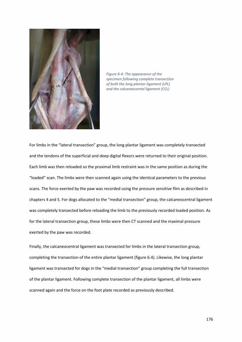
176

For limbs in the “lateral transection” group, the long plantar ligament was completely transected

and the tendons of the superficial and deep digital flexors were returned to their original position.

Each limb was then reloaded so the proximal limb restraint was in the same position as during the

“loaded” scan. The limbs were then scanned again using the identical parameters to the previous

scans. The force exerted by the paw was recorded using the pressure sensitive film as described in

chapters 4 and 5. For dogs allocated to the “medial transection” group, the calcaneocentral ligament

was completely transected before reloading the limb to the previously recorded loaded position. As

for the lateral transection group, these limbs were then CT scanned and the maximal pressure

exerted by the paw was recorded.

Finally, the calcaneocentral ligament was transected for limbs in the lateral transection group,

completing the transection of the entire plantar ligament (figure 6.4). Likewise, the long plantar

ligament was transected for dogs in the “medial transection” group completing the full transection

of the plantar ligament. Following complete transection of the plantar ligament, all limbs were

scanned again and the force on the foot plate recorded as previously described.

LPL

CCL

Figure 6-4: The appearance of the specimen following complete transection of both the long plantar ligament (LPL) and the calcaneocental ligament (CCL)

177

6.2.6 Calculation of kinematics

A previously validated CT based technique for measuring canine tarsal bone kinematics (Tan et al.,

2017), previously outlined in chapters 3 and 5 was used. Briefly, a 3D bone model was generated for

the calcaneus, talus, fourth, third and second tarsal bones, central tarsal bone and metatarsal bones

II, III, IV and V for every scan. The bones were then aligned to an anatomically based co-ordinate

system that would allow motions to be described using conventional descriptors. Rotation around

the y axis represented dorsiflexion and plantarflexion, rotation around the x axis represented

internal and external rotation, whilst rotation around the z axis represented either valgus or varus

angulation (figure 6.5). The position of each bone was recorded in an unloaded position, a loaded

position, a position after transection of the medial or lateral portion of the plantar ligament and a

position following full transection of the plantar ligament. The displacement of each bone relative to

its unloaded position was reported for each condition (loaded, partial transection and full

transection). Bone displacement was described using 6 degrees of freedom (3 translations along the

co-ordinate axes and 3 rotations around the same axes). As in the previous chapters, individual bone

motion was also reported as a total summative rotation (total rotation) around a single axis, which

was termed the helical axis of rotation.

178

6.2.7 Data analysis

The two groups (medial and lateral transection) were compared for two different conditions (intact

and following sectioning of the plantar ligament). Initially, the groups were compared following

application of a load to the intact limbs. A paired t-test was used to compare the force exerted on

the footplate, hock angle and the motion of individual bones between groups using Excel (Microsoft,

Redmond, Washington, USA). The two groups were again compared using the same parameters

following complete transection of the plantar ligament.

Figure 6-5: The three reference axes around which all motions are described. Left: Positive and negative values are reported indicating the direction of the rotations around the axes. For rotations around the X axis, calculations have been adjusted so positive values translate to an external rotation for both left and right limbs. For rotations around the Z axis, calculations have been adjusted so positive values translate to adduction for both left and right limbs No adjustment is required for rotations around the Y axis. Right: Positive and negative values are reported indicating the direction of the translation along the axes. For translation along the Y axis, calculations have been adjusted so positive translations always indicate a medial direction for both left and right limbs. No adjustment is required for translation along the other axes.

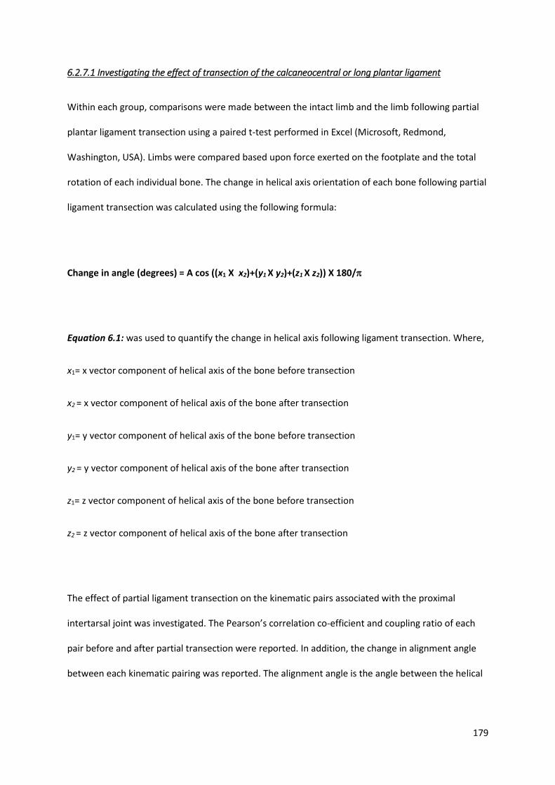
179

6.2.7.1 Investigating the effect of transection of the calcaneocentral or long plantar ligament

Within each group, comparisons were made between the intact limb and the limb following partial

plantar ligament transection using a paired t-test performed in Excel (Microsoft, Redmond,

Washington, USA). Limbs were compared based upon force exerted on the footplate and the total

rotation of each individual bone. The change in helical axis orientation of each bone following partial

ligament transection was calculated using the following formula:

Change in angle (degrees) = A cos ((x1 X x2)+(y1 X y2)+(z1 X z2)) X 180/

Equation 6.1: was used to quantify the change in helical axis following ligament transection. Where,

x1= x vector component of helical axis of the bone before transection

x2 = x vector component of helical axis of the bone after transection

y1= y vector component of helical axis of the bone before transection

y2 = y vector component of helical axis of the bone after transection

z1= z vector component of helical axis of the bone before transection

z2 = z vector component of helical axis of the bone after transection

The effect of partial ligament transection on the kinematic pairs associated with the proximal

intertarsal joint was investigated. The Pearson’s correlation co-efficient and coupling ratio of each

pair before and after partial transection were reported. In addition, the change in alignment angle

between each kinematic pairing was reported. The alignment angle is the angle between the helical

180

axis of one bone in the kinematic pair and the helical axis of the other bone in the pair and was

calculated using the following equation:

Alignment angle (AA) (degrees) = A cos ((x1 X x2)+(y1 X y2)+(z1 X z2)) X 180/

Equation 6.2: Calculation of the alignment angle

Where,

x1= x vector component of helical axis of bone 1

x2 = x vector component of helical axis of bone 2

y1= y vector component of helical axis of bone 1

y2 = y vector component of helical axis of bone 2

z1= z vector component of helical axis of bone 1

z2 = z vector component of helical axis of bone 2

Kinematic pairs with a low alignment angle therefore move in the same direction during loading.

181

6.3 Results

6.3.1 Comparison of groups before transection

There were 5 limbs assigned to each group. The mean force recorded on the footplate for the medial

transection group (1013±155N, mean ± SD) was not different to the force recorded from the lateral

transection group (1055±140N) (p= 0.44).

The mean hock angle recorded for the intact limb of the medial transection group (85.5 ± 3.2

degrees, mean ± SD) was not different to hock angle recorded for the intact limb of the lateral

transection group (87.9 ± 2.9 degrees) (p= 0.1)

For all limbs, each bone underwent rotations around and translations along each of the 3 reference

axes. There was no difference in rotation or translation of any bone along or around any of the axes

between groups. Similarly, there was no difference in the total rotation of any bone between

groups. The three vectors defining the helical axis of each bone were not different between the two

groups (tables 6.1 and 6.2).

182

Table 6-1: motion of each bone following application of a load to the intact limb (medial transection group). Rotations and translations can be seen to occur along and around all three reference axes. CTB = central tarsal bone, TB = tarsal bone, MT = metatarsal bone, SD = standard deviation.

Table 6-2: motion of each bone following application of a load to the intact limb (lateral transection group). Rotations and translations can be seen to occur along and around all three reference axes. CTB = central tarsal bone, TB = tarsal bone, MT = metatarsal bone, SD = standard deviation.

x axis y axis z axis x axis y axis z axis

mean 38.45 2.72 15.08 1.91 -28.23 2.80 28.51

SD 5.17 3.41 3.99 2.45 2.95 2.13 2.87

mean 0.45 0.43 0.13 -2.90 2.28 -0.82 3.90

SD 0.28 0.08 0.18 1.56 1.46 0.47 2.05

mean 0.22 0.84 1.08 -2.07 4.80 -1.21 5.46

SD 0.14 0.23 0.44 0.90 2.04 0.59 2.07

mean 0.37 1.20 1.96 -2.13 5.07 -1.50 5.79

SD 0.20 0.30 0.85 0.80 2.53 0.30 2.51

mean 0.15 1.27 2.21 -1.19 6.17 -1.66 6.59

SD 0.17 0.34 0.93 0.77 2.33 0.61 2.29

mean 0.32 1.24 1.96 -2.04 6.08 -0.39 6.88

SD 0.16 0.30 0.88 0.86 2.07 2.56 2.00

mean 0.01 2.94 9.12 1.78 11.18 -1.95 11.52

SD 0.47 0.63 3.17 0.77 3.44 0.47 3.29

mean -0.92 3.18 10.49 1.41 11.86 -2.01 12.13

SD 0.67 0.81 3.43 0.63 3.30 0.70 3.20

mean -0.96 3.35 10.34 -2.08 11.82 -2.87 12.52

SD 0.65 0.83 3.43 1.67 3.15 0.93 3.06

mean -0.31 3.43 10.15 -1.90 11.43 -2.85 12.14

SD 0.39 0.71 3.06 2.10 2.77 0.79 2.76

total rotation

(degrees)

MT IV

MT V

Calcaneus

translation along (mm) rotation around (degrees)

CTB

Fourth TB

Third TB

Second TB

MT II

MT III

Tibia

Medial transection group:

Intact limb

x axis y axis z axis x axis y axis z axis

mean 37.20 2.98 15.20 1.95 -28.98 3.49 29.23

SD 5.86 2.40 3.51 1.65 3.94 0.99 3.90

mean 0.38 0.37 0.15 -2.52 1.81 -0.71 3.27

SD 0.34 0.10 0.20 1.50 1.65 0.48 2.17

mean 0.22 0.76 0.98 -1.77 4.32 -1.14 4.85

SD 0.19 0.23 0.50 0.71 2.33 0.48 2.43

mean 0.32 1.09 1.73 -2.01 4.44 -1.51 5.15

SD 0.26 0.36 0.95 0.75 2.33 0.37 2.41

mean 0.15 1.18 2.04 -1.06 5.81 -1.77 6.20

SD 0.17 0.33 1.05 0.70 2.53 0.72 2.66

mean 0.32 1.16 1.85 -0.77 5.54 -1.57 5.89

SD 0.20 0.36 1.02 0.42 3.11 0.92 3.12

mean 0.17 2.89 8.56 1.89 10.50 -2.11 10.96

SD 0.04 0.85 2.99 1.53 3.13 0.82 3.09

mean -0.78 3.21 9.95 2.01 11.39 -2.20 11.80

SD 0.29 0.89 3.54 1.05 3.27 0.78 3.22

mean -0.85 3.50 9.67 -1.85 11.26 -3.34 12.00

SD 0.29 0.82 3.49 1.46 3.18 0.55 3.29

mean -0.33 3.50 9.41 -1.96 10.78 -3.18 11.51

SD 0.15 0.79 3.08 1.27 2.76 0.55 2.89

translation along (mm) rotation around (degrees) total rotation

(degrees)

CTB

MT IV

MT V

Fourth TB

Third TB

Second TB

MT II

MT III

Lateral transection group:

Intact limb

Tibia

Calcaneus

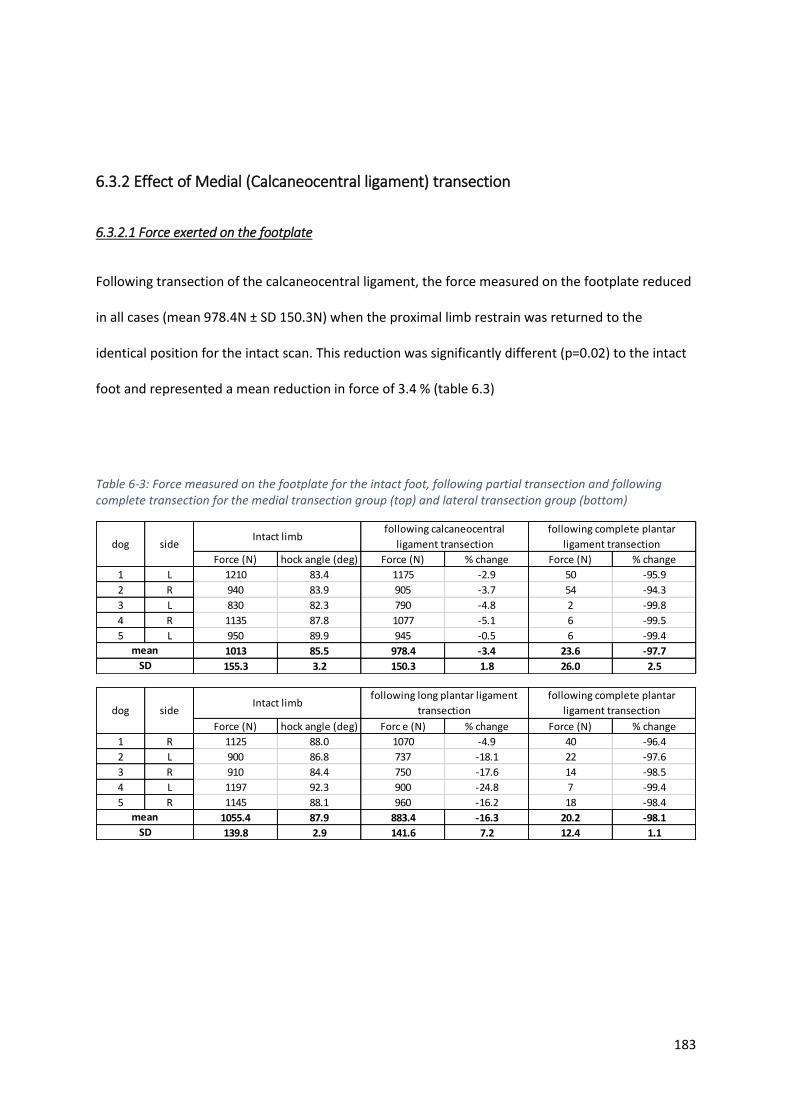
183

6.3.2 Effect of Medial (Calcaneocentral ligament) transection

6.3.2.1 Force exerted on the footplate

Following transection of the calcaneocentral ligament, the force measured on the footplate reduced

in all cases (mean 978.4N ± SD 150.3N) when the proximal limb restrain was returned to the

identical position for the intact scan. This reduction was significantly different (p=0.02) to the intact

foot and represented a mean reduction in force of 3.4 % (table 6.3)

Table 6-3: Force measured on the footplate for the intact foot, following partial transection and following complete transection for the medial transection group (top) and lateral transection group (bottom)

Force (N) hock angle (deg) Force (N) % change Force (N) % change

1 L 1210 83.4 1175 -2.9 50 -95.9

2 R 940 83.9 905 -3.7 54 -94.3

3 L 830 82.3 790 -4.8 2 -99.8

4 R 1135 87.8 1077 -5.1 6 -99.5

5 L 950 89.9 945 -0.5 6 -99.4

1013 85.5 978.4 -3.4 23.6 -97.7

155.3 3.2 150.3 1.8 26.0 2.5

sidedog

mean

SD

Intact limbfollowing calcaneocentral

ligament transection

following complete plantar

ligament transection

Force (N) hock angle (deg) Forc e (N) % change Force (N) % change

1 R 1125 88.0 1070 -4.9 40 -96.4

2 L 900 86.8 737 -18.1 22 -97.6

3 R 910 84.4 750 -17.6 14 -98.5

4 L 1197 92.3 900 -24.8 7 -99.4

5 R 1145 88.1 960 -16.2 18 -98.4

1055.4 87.9 883.4 -16.3 20.2 -98.1

139.8 2.9 141.6 7.2 12.4 1.1

mean

SD

dog sideIntact limb

following long plantar ligament

transection

following complete plantar

ligament transection

184

6.3.2.2 Total rotation

For all bones investigated, both a total rotation and 6 degrees of freedom motion was recorded

following transection of the calcaneocentral ligament (table 6.4)

Table 6-4: Motion of each bone following application of a load to the limb after transection of the calcaneocentral ligament (medial transection group). Rotations and translations can be seen to occur along and around all three reference axes. CTB = central tarsal bone, TB = tarsal bone, MT = metatarsal bone, SD = standard deviation.

When the total rotation of each bone following transection was compared to the motion in the

intact foot, all tarsal and metatarsal bones showed a significantly greater rotation following

transection of the calcaneocentral ligament. Conversely, the tibial rotation was reduced in all dogs

following calcaneocentral ligament transection (fig 6.6)

x axis y axis z axis x axis y axis z axis

mean 36.68 2.99 14.71 2.08 -26.98 2.97 27.28

SD 5.20 3.24 3.76 2.27 3.00 1.96 2.94

mean 0.55 0.56 0.10 -3.43 3.15 -0.66 4.80

SD 0.28 0.13 0.18 1.57 1.36 0.35 2.02

mean 0.32 1.09 1.53 -1.03 6.88 -2.20 7.46

SD 0.24 0.32 0.44 0.91 2.46 1.01 2.29

mean 0.46 1.41 2.40 -1.09 6.29 -1.89 6.78

SD 0.24 0.33 0.82 0.97 2.61 0.38 2.50

mean 0.22 1.60 2.91 -0.10 7.89 -2.54 8.39

SD 0.23 0.44 0.96 0.91 2.38 0.88 2.24

mean 0.32 1.70 2.53 -4.20 5.63 -3.54 11.44

SD 0.33 0.45 1.11 7.26 5.12 4.81 4.03

mean -0.04 3.84 11.34 3.16 13.30 -2.95 13.98

SD 0.59 0.84 3.45 0.98 3.78 0.62 3.58

mean -1.17 4.27 12.63 2.92 13.78 -3.06 14.40

SD 0.86 0.97 3.69 0.89 3.66 0.76 3.52

mean -1.17 4.34 12.08 -0.64 13.45 -3.93 14.22

SD 0.80 0.89 3.51 2.27 3.32 0.93 3.26

mean -0.44 4.29 11.74 -0.69 13.08 -3.92 13.93

SD 0.50 0.65 3.12 2.67 2.97 0.74 2.87

Second TB

MT II

MT III

MT IV

translation (mm) rotation (degrees) total rotation

around helical axis

(degrees)

Medial transection group:

Following calcaneocentral

ligament transection

MT V

Tibia

Calcaneus

CTB

Fourth TB

Third TB

185

Figure 6-6: Comparison of total rotation of each bone before and after calcaneocentral ligament transection. For all tarsal and metatarsal bones, there is a significant increase in the magnitude of rotation following transection of the calcaneocentral ligament, suggesting the calcaneocentral ligament plays an important role in stability across the entire proximal intertarsal joint. Error bars represent one standard deviation. CTB = central tarsal bone, TB = tarsal bone, MT = metatarsal bone.* denotes significant difference (p-value)

0.00

5.00

10.00

15.00

20.00

25.00

30.00

35.00

Tibia Calcaneus CTB Fourth TB Third TB Second TB MT II MT III MT IV MT V

Tota

l ro

tati

on

(deg

rees

)

Bone

Effect of calcaneocentral ligament transection on total rotation

Intact limb post transection

*p=0.00

*p=0.00 *p=0.00 *p=0.00

*p=0.00

p=0.07 *p=0.00

*p=0.04

*p=0.00

*p=0.00

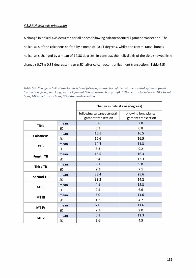
186

6.3.2.3 Helical axis orientation

A change in helical axis occurred for all bones following calcaneocentral ligament transection. The

helical axis of the calcaneus shifted by a mean of 10.11 degrees, whilst the central tarsal bone’s

helical axis changed by a mean of 14.38 degrees. In contrast, the helical axis of the tibia showed little

change ( 0.78 ± 0.35 degrees; mean ± SD) after calcaneocentral ligament transection. (Table 6.5)

Table 6-5: Change in helical axis for each bone following transection of the calcaneocentral ligament (medial transection group) and long plantar ligament (lateral transection group). CTB = central tarsal bone, TB = tarsal bone, MT = metatarsal bone, SD = standard deviation.

change in helical axis (degrees)

following calcaneocentral ligament transection

following long plantar ligament transection

Tibia mean 0.8 2.8

SD 0.3 0.8

Calcaneus mean 10.1 16.5

SD 10.6 16.5

CTB mean 14.4 11.3

SD 3.3 9.2

Fourth TB mean 13.5 16.3

SD 6.4 12.3

Third TB mean 9.1 9.8

SD 2.2 7.1

Second TB mean 38.4 25.6

SD 38.2 14.2

MT II mean 4.1 12.3

SD 0.5 6.6

MT III mean 5.0 11.6

SD 1.2 4.7

MT IV mean 7.0 11.6

SD 2.3 2.0

MT V mean 6.1 12.3

SD 2.6 4.5

187

6.3.2.4 Kinematic pairs of the proximal intertarsal joint

The kinematic pairs evaluated were the calcaneus and central tarsal bone, the calcaneus and fourth

tarsal bone and the central tarsal bone and 4th tarsal bone.

The strong linear kinematic coupling between total rotation of the calcaneus and central tarsal bone

(R2 = 0.99 in the intact limb) remained high following calcaneocentral ligament transection (R2 =

0.93) and this was similarly seen the calcaneus/fourth tarsal bone pairing and the Central/fourth

tarsal bone pairing (table 6.6).

The alignment angle(AA) between the helical axis of the calcaneus and central tarsal bone was

significantly different (p=0.047) between the intact limb (AA= 31.46 ± 17.25 degrees) and the limb

following calcaneocentral ligament transection (38.64 ± 12.39 degrees). A significant difference

(p=0.004) was also seen in the alignment axis of the calcaneus and fourth tarsal bone between

conditions. The partial transection produced no significant difference in the AA of the central and

fourth tarsal bones (p=0.24) (table 6.6).

Table 6-6: Comparison of the alignment axis, coupling ration and correlation coefficient for three pairs of bones associated with the PIT joint in the intact limbs, following partial transection and following complete transection of the plantar ligament. The small values of the alignment angle for the CTB and fourth tarsal bone pairing suggest that these bones always rotate around a very similar axis for all conditions consistent with a functional rigid unit.

CTB = central tarsal bone, 4th = fourth tarsal bone

correlation

coefficient

(R2)

coupling

ratio

alignment

angle of

helical axes

(degrees)

correlation

coefficient

(R2)

coupling

ratio

alignment

angle of

helical axes

(degrees)

correlation

coefficient

(R2)

coupling

ratio

alignment

angle of

helical axes

(degrees)

correlation

coefficient

(R2)

coupling

ratio

alignment

angle of

helical axes

(degrees)

Calcaneus and CTB 0.99 1.06 33.7 0.93 1.09 38.64 0.98 1.09 43.96 0.03 0.41 55.22

Calcaneus and 4th 0.98 1.15 32.45 0.97 1.22 37.61 0.99 1.13 50.83 0.04 0.46 56.24

CTB and 4th 0.98 1.08 5.62 0.97 1.07 4.01 0.99 1.02 8.48 0.98 0.91 2.22

Pair of bones

Intact limbFollowing calcaneocentral ligament

transection

Following long plantar ligament

transection

following complete transection of

plantar ligament

condition

188

6.3.3 Effect of Lateral (Long plantar ligament) transection

6.3.3.1 Force exerted on the footplate

Following transection of the long plantar ligament, the force measured on the footplate reduced in

all cases (mean 883.4N; SD 141.6N) when the proximal limb restrain was returned to the identical

position for the intact scan. This reduction was significantly different (p=0.01) to the intact foot and

represented a mean reduction in force of 16.3 % (table 6.3)

6.3.3.2 Total rotation

For all bones investigated, both a total rotation and 6 degrees of freedom motion was recorded

following transection of the long plantar ligament (table 6.7).

189

Table 6-7: Motion of each bone following application of a load to the limb after transection of the long plantar ligament (lateral transection group). CTB = central tarsal bone, TB = tarsal bone, MT = metatarsal bone, SD = standard deviation.

Following transection of the long plantar ligament, there was a significant decrease in rotation of the

tibia and a significant increase in rotation of all other bones, with the exception of the calcaneus,

which showed no significant difference in rotation to the intact foot (figure 6.7)

x axis y axis z axis x axis y axis z axis

mean 34.09 2.82 14.67 1.75 -26.75 3.06 26.97

SD 5.88 1.96 3.18 1.42 4.10 0.94 4.08

mean 0.43 0.22 0.05 -2.20 1.45 -0.95 2.93

SD 0.30 0.06 0.15 1.64 1.68 0.55 2.26

mean 0.29 1.05 1.40 -1.98 6.23 -1.89 6.86

SD 0.14 0.21 0.48 0.81 2.38 0.46 2.50

mean 0.69 1.40 2.66 -1.69 9.29 -2.31 9.85

SD 0.19 0.36 1.00 1.45 2.50 0.72 2.55

mean 0.25 1.51 3.10 -1.55 8.32 -2.32 8.83

SD 0.13 0.32 1.02 0.88 2.34 0.73 2.50

mean 0.48 1.52 2.76 -2.05 8.59 -0.93 9.12

SD 0.16 0.30 1.00 0.77 2.41 2.22 2.50

mean 0.14 3.19 11.26 0.40 13.00 -1.89 13.26

SD 0.23 0.86 2.83 1.72 2.80 0.84 2.75

mean -1.06 3.42 13.22 -0.15 14.10 -2.00 14.32

SD 0.44 0.83 3.36 1.38 2.97 0.68 2.96

mean -1.24 3.85 13.78 -4.36 14.95 -3.23 16.04

SD 0.50 0.72 3.38 1.15 2.84 0.27 2.89

mean -0.50 4.16 13.99 -4.14 15.02 -3.32 16.05

SD 0.39 0.77 3.01 0.97 2.55 0.42 2.67

MT IV

MT V

Fourth TB

Third TB

Second TB

MT II

MT III

Lateral transection group:

Following long plantar ligament

transection

Tibia

Calcaneus

CTB

translation (mm) rotation (degrees) total rotation

around helical axis

(degrees)

190

Figure 6-7: Comparison of total rotation of each bone before and after long plantar ligament transection. For all tarsal and metatarsal bones, there is a significant increase in the magnitude of rotation following transection of the long plantar ligament, suggesting the long plantar ligament plays an important role in stability across the entire proximal intertarsal joint. Error bars denote one standard deviation. CTB = central tarsal bone, TB = tarsal bone, MT = metatarsal bone. * denotes significant difference (p-value)

0.00

5.00

10.00

15.00

20.00

25.00

30.00

35.00

Tibia Calcaneus CTB Fourth TB Third TB Second TB MT II MT III MT IV MT V

Tota

l ro

tati

on

(deg

rees

)

Bone

Effect of long plantar ligament transection on total rotation

Intact limb post transection

*p=0.00

p=0.17

*p=0.00*p=0.00

*p=0.00

*p=0.00

*p=0.00 *p=0.00

*p=0.00

*p=0.00 *p=0.00 *p=0.00

191

6.3.3.3 Helical axis orientation

As with the medial transection group, a change in the helical axis around which each bone rotated

occurred for all bones following long plantar ligament transection (table 6.5)

6.3.3.4 Kinematic pairs of the proximal intertarsal joint

The strong linear kinematic coupling between total rotation of the calcaneus and central tarsal bone

(R2 = 0.99 in the intact limb) remained high following transection of the long plantar ligament (R2 =

0.98) and this was similarly seen the calcaneus/fourth tarsal bone pairing and the Central/fourth

tarsal bone pairing (table 6.6).

The alignment angle between the helical axis of the calcaneus and central tarsal bone increased

between the intact limb (AA= 35.96 ± 17.49 degrees) and the limb following transection of the long

plantar ligament (43.96 ± 22.44 degrees) was not significantly different (p=0.06). A significant

difference (p=0.01) was seen in the alignment axis of the calcaneus and fourth tarsal bone between

conditions. The partial transection produced no significant difference in the AA of the central and

fourth tarsal bones (p=0.16) (table 6.6).

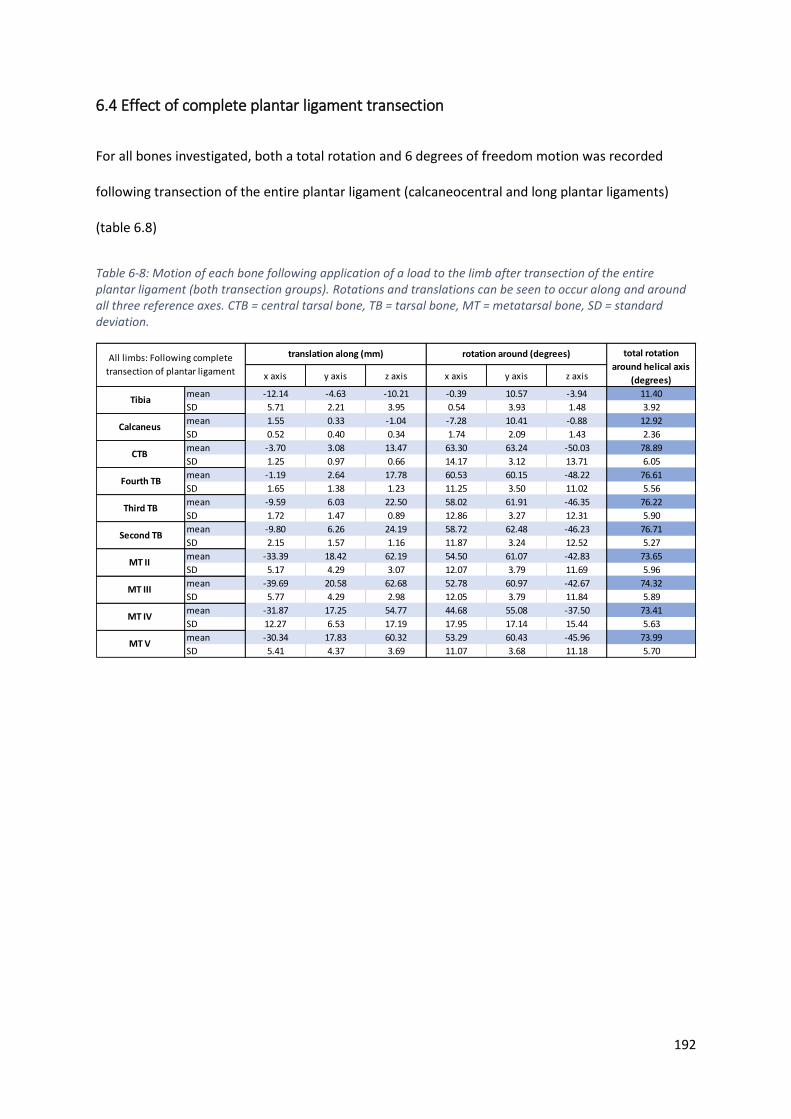
192

6.4 Effect of complete plantar ligament transection

For all bones investigated, both a total rotation and 6 degrees of freedom motion was recorded

following transection of the entire plantar ligament (calcaneocentral and long plantar ligaments)

(table 6.8)

Table 6-8: Motion of each bone following application of a load to the limb after transection of the entire plantar ligament (both transection groups). Rotations and translations can be seen to occur along and around all three reference axes. CTB = central tarsal bone, TB = tarsal bone, MT = metatarsal bone, SD = standard deviation.

x axis y axis z axis x axis y axis z axis

mean -12.14 -4.63 -10.21 -0.39 10.57 -3.94 11.40

SD 5.71 2.21 3.95 0.54 3.93 1.48 3.92

mean 1.55 0.33 -1.04 -7.28 10.41 -0.88 12.92

SD 0.52 0.40 0.34 1.74 2.09 1.43 2.36

mean -3.70 3.08 13.47 63.30 63.24 -50.03 78.89

SD 1.25 0.97 0.66 14.17 3.12 13.71 6.05

mean -1.19 2.64 17.78 60.53 60.15 -48.22 76.61

SD 1.65 1.38 1.23 11.25 3.50 11.02 5.56

mean -9.59 6.03 22.50 58.02 61.91 -46.35 76.22

SD 1.72 1.47 0.89 12.86 3.27 12.31 5.90

mean -9.80 6.26 24.19 58.72 62.48 -46.23 76.71

SD 2.15 1.57 1.16 11.87 3.24 12.52 5.27

mean -33.39 18.42 62.19 54.50 61.07 -42.83 73.65

SD 5.17 4.29 3.07 12.07 3.79 11.69 5.96

mean -39.69 20.58 62.68 52.78 60.97 -42.67 74.32

SD 5.77 4.29 2.98 12.05 3.79 11.84 5.89

mean -31.87 17.25 54.77 44.68 55.08 -37.50 73.41

SD 12.27 6.53 17.19 17.95 17.14 15.44 5.63

mean -30.34 17.83 60.32 53.29 60.43 -45.96 73.99

SD 5.41 4.37 3.69 11.07 3.68 11.18 5.70

Second TB

MT II

MT III

MT IV

translation along (mm) rotation around (degrees) total rotation

around helical axis

(degrees)

All limbs: Following complete

transection of plantar ligament

MT V

Tibia

Calcaneus

CTB

Fourth TB

Third TB

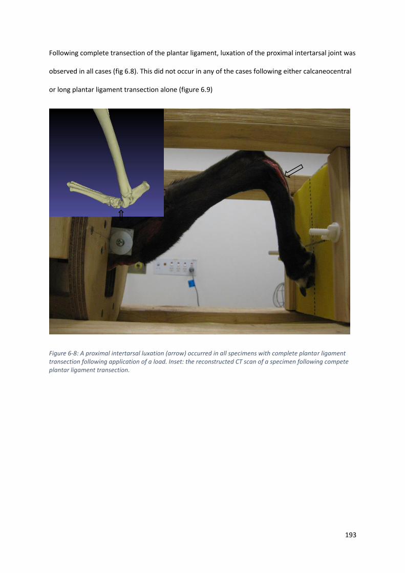
193

Following complete transection of the plantar ligament, luxation of the proximal intertarsal joint was

observed in all cases (fig 6.8). This did not occur in any of the cases following either calcaneocentral

or long plantar ligament transection alone (figure 6.9)

Figure 6-8: A proximal intertarsal luxation (arrow) occurred in all specimens with complete plantar ligament transection following application of a load. Inset: the reconstructed CT scan of a specimen following compete plantar ligament transection.

194

Figure 6-9: Effects of ligament transection on bone position. Top row: The position of bones of the pes of for a dog in the medial transection group before transection (A), after transection of the calcaneocentral ligament (yellow bones, B) and after complete plantar ligament transection (green bones, C). Bottom row: The position of bones of the pes of for a dog in the lateral transection group before transection (D), after transection of the long plantar ligament (pink bones, E) and after complete plantar ligament transection (green bones, F). Note the speckled appearance of the talus in the superimposed examples as this represents the reference bone that all other motion is described.

The mean force recorded on the footplate for dogs after complete plantar ligament transection was

23.6N (± SD 26.0N), representing a mean reduction in force of 97.7% for the medial transection

group and 22.2N (± 12.4N), representing a mean reduction in force of 98.0% for the lateral

transection group (table 6.3).

A

v

B

vv

C

vv

E

vv

vC

V

C

V

D

vv

F

vv

vC

V

C

V

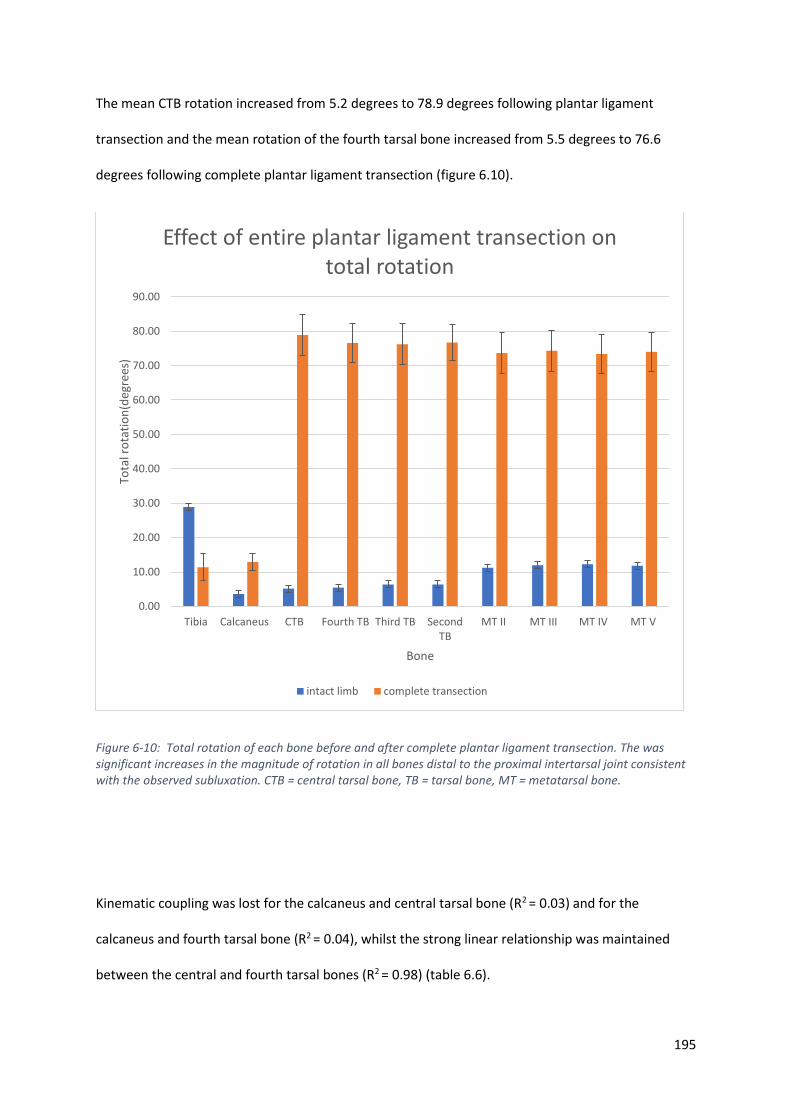
195

The mean CTB rotation increased from 5.2 degrees to 78.9 degrees following plantar ligament

transection and the mean rotation of the fourth tarsal bone increased from 5.5 degrees to 76.6

degrees following complete plantar ligament transection (figure 6.10).

Figure 6-10: Total rotation of each bone before and after complete plantar ligament transection. The was significant increases in the magnitude of rotation in all bones distal to the proximal intertarsal joint consistent with the observed subluxation. CTB = central tarsal bone, TB = tarsal bone, MT = metatarsal bone.

Kinematic coupling was lost for the calcaneus and central tarsal bone (R2 = 0.03) and for the

calcaneus and fourth tarsal bone (R2 = 0.04), whilst the strong linear relationship was maintained

between the central and fourth tarsal bones (R2 = 0.98) (table 6.6).

0.00

10.00

20.00

30.00

40.00

50.00

60.00

70.00

80.00

90.00

Tibia Calcaneus CTB Fourth TB Third TB SecondTB

MT II MT III MT IV MT V

Tota

l ro

tati

on

(deg

rees

)

Bone

Effect of entire plantar ligament transection on total rotation

intact limb complete transection

196

6.4 Discussion

To date, the role of plantar ligament in maintaining the stability within the pes has received little

attention and most descriptions are based upon anatomical assumptions. The results of this chapter

have identified that the plantar ligament is the only ligamentous structure that prevents subluxation

of the proximal intertarsal joint during weight bearing. Furthermore, the results demonstrate that in

this cadaveric model of ligamentous injury, loss of either the long plantar or calcaneocentral

ligament alone does not produce proximal intertarsal subluxation and still allows continued force

transmission through this limb segment, although at reduced levels.

6.4.1 Anatomy of the plantar ligament

The anatomical appearance of the plantar ligament was consistent with previous descriptions (Evans

et al., 2012) (Arwedsson, 1954) (Carmichael and Marshall, 2013) (Holt, 1974), being comprised of

two main parts, the calcaneocentral and long plantar ligaments, and a third smaller but distinctive

fibrous band arising from the caudolateral aspect of the calcaneus to insert with the m. peroneus

brevis on the head of the fifth metatarsal bone (figure 6.11). This distinctive fibrous band has been

termed the primarily tendinous muscle abductor digiti V by some authors (Arwedsson, 1954; Evans

et al., 2012; Holt, 1974), whilst others have included this band as the third component of the plantar

ligament, referring to it as the calcaneoquartal ligament (Evans et al., 2012) or the lateral plantar

ligament (Carmichael and Marshall, 2013).

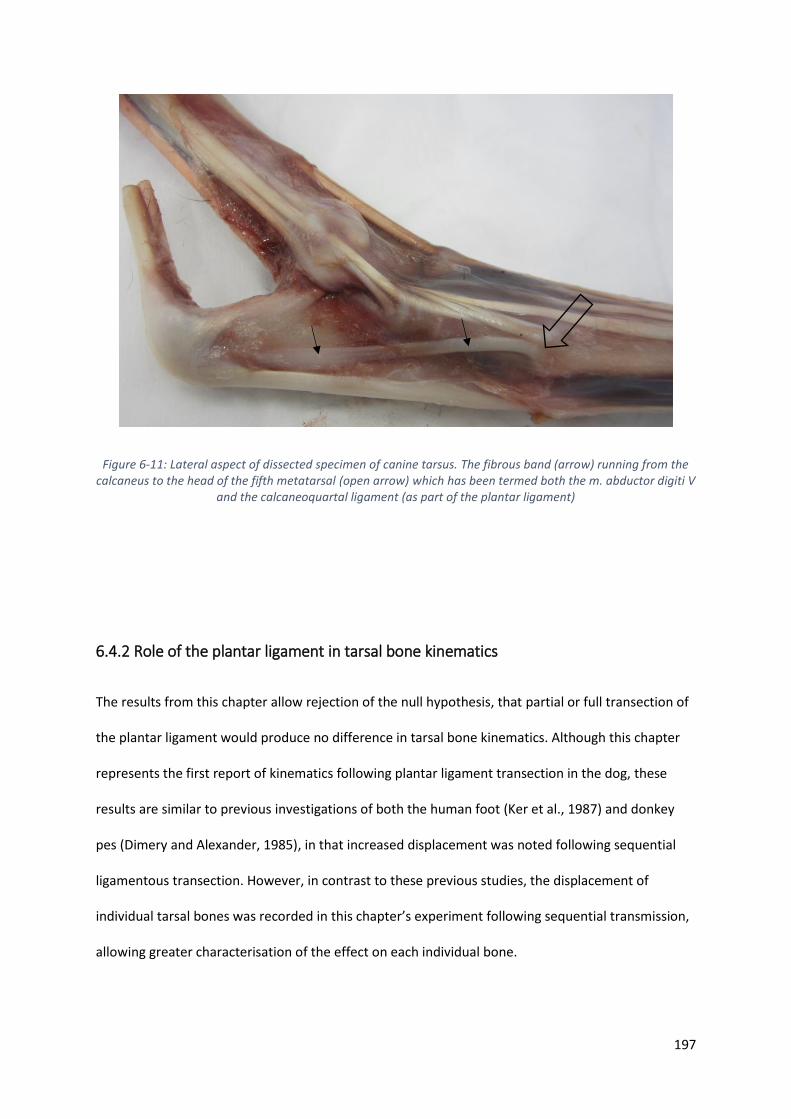
197

Figure 6-11: Lateral aspect of dissected specimen of canine tarsus. The fibrous band (arrow) running from the calcaneus to the head of the fifth metatarsal (open arrow) which has been termed both the m. abductor digiti V

and the calcaneoquartal ligament (as part of the plantar ligament)

6.4.2 Role of the plantar ligament in tarsal bone kinematics

The results from this chapter allow rejection of the null hypothesis, that partial or full transection of

the plantar ligament would produce no difference in tarsal bone kinematics. Although this chapter

represents the first report of kinematics following plantar ligament transection in the dog, these

results are similar to previous investigations of both the human foot (Ker et al., 1987) and donkey

pes (Dimery and Alexander, 1985), in that increased displacement was noted following sequential

ligamentous transection. However, in contrast to these previous studies, the displacement of

individual tarsal bones was recorded in this chapter’s experiment following sequential transmission,

allowing greater characterisation of the effect on each individual bone.

198

As the central and fourth tarsal bones have no direct muscular attachments(Evans et al., 2012), it is

perhaps not surprising that an increase in rotation was seen following ligament transection, since

ligaments, along with the joint surface shape, provide the major restraints to bone motion

(Sennwald et al., 1993). However, the findings of this chapter also revealed significant changes in

both the magnitude of total rotation and orientation of the helical axis of all bones and not just

those associated with the proximal intertarsal joints. The bones of the pes form a kinematic chain

both along the longitudinal axis of the foot and across it. Changes in the motion of one bone had a

significant effect on all bones further suggesting that the pes works as a single co-ordinated limb

segment, consistent with the results of the previous chapter.

Tarsal bone motions are particularly dependant on the movement of adjacent bones, which directly

influence the compressive forces across articular surfaces and the tensile forces produced by

ligamentous attachments. In the human foot, arthrodesis of any of the joints of the triple joint

complex (the subtalar, talonavicular, and calcaneocuboid joints) limits the motion of the

remaining, unfused joints (Astion et al., 1997) highlighting the interdependence of tarsal bone

motions. Although the same experiments have not been repeated in dogs, the finding of this present

study suggest that there is also an interdependence of tarsal bone motion. Injuries or interventions

that alter motion at one intertarsal joint are likely to affect surrounding joints of the pes by altering

the magnitude of rotation of a bone or altering the helical axis around which that bone rotates.

Following transection of the long plantar ligament, excessive rotation of the central tarsal bone and

fourth tarsal bone (termed the midfoot functional unit in the previous chapter) is prevented by the

calcaneocentral component of the plantar ligament and remaining joint capsule. Although the

magnitude of rotation of the midfoot unit is increased, excessive rotation of the fourth tarsal bone is

prevented despite complete loss of the plantar attachment to the proximal bone, the calcaneus. For

this to occur, the strong ligamentous attachments between the central and fourth tarsal bones must

remain intact.

199

Similarly, following transection of the calcaneocentral ligament, subluxation of the central tarsal

bone was prevented by its strong attachments to the fourth tarsal bone and surrounding joint

capsule.

6.4.3 Role of the plantar ligament in energy storage and transmission

In the previous chapter, the elastic dorsiflexion of the canine pes was suggested as a means of

storing and transmitting energy within the limb segment. This has been demonstrated in other

species including humans and equids (Dimery and Alexander, 1985; Ker et al., 1987).

The findings of this chapter suggest all aspects of the plantar ligament contribute to the transmission

of force through the canine pes. Partial transection of different aspects of the ligament produced a

significant reduction in force that could be transmitted through the pes, however, subluxation or

luxation did not occur until the entire plantar ligament was transected (figure 6.7), suggesting that

disruption to both the long plantar ligament and calcaneocentral ligament are required before

proximal intertarsal subluxation occurs, supporting previous suggestions (Allen et al., 1993; Barnes

et al., 2013; Campbell et al., 1976; Lawson, 1960). Proximal intertarsal subluxation was possible

despite the presence of an intact tendinous abductor digiti V (also termed lateral plantar ligament or

calcaneoquartal ligament), suggesting that it contributes little to stability across these joints.

This chapter represents the first known kinematic study of the canine pes and comparisons can only

be made to kinematic investigations involving different species, which often exhibit significant

variation in anatomy and stance. The bones of the plantigrade human foot were shown to store less

elastic energy following transection of the long and short plantar ligaments and calcaneonavicular

(spring) ligament (which runs in a similar direction to the calcaneocentral ligament) (Ker et al., 1987).

Similar to the findings of this chapter, subluxation did not occur after transection of only

components of the plantar ligamentous support. A sequential transection of tendons of the pes of

200

the donkey demonstrated a reduced ability to store elastic energy in the pes, however, transection

of plantar ligaments was not performed (Dimery and Alexander, 1985).

The paired study design of this chapter allowed direct comparison between the role of the long

plantar ligament and the calcaneocentral plantar ligament in force transmission through the pes.

The loss of the integrity of long plantar ligament results in a greater loss in force transmission

compared to the loss of integrity of the calcaneocentral ligament, suggesting the former plays a

greater role in force transmission within the pes. This information may be important when

attempting to re-establish integrity of the pes following proximal intertarsal subluxation. Previous

clinical reports suggest that stabilisation of the calcaneoquartal joint alone may be adequate despite

subluxation of the talocentral joint, which occurs concurrently during proximal intertarsal

subluxation (Allen et al., 1993; Barnes et al., 2013; Campbell et al., 1976; Lawson, 1960)

6.4.5 Clinical importance

The clinical importance of these findings relates to conditions whereby the integrity of the plantar

ligament is lost, either through trauma or degenerative processes. Proximal intertarsal (PIT) joint

subluxation in well described and breeds such as Shetland sheepdogs and Collies are over-

represented (Allen et al., 1993; Barnes et al., 2013; Campbell et al., 1976; Fettig et al., 2002). In many

cases, degeneration of the plantar ligament is suspected, and many animals experience an insidious

onset without a history of major trauma (Campbell et al., 1976). The ability to redirect force through

the pes following the loss of approximately 50% of the plantar ligament, as demonstrated in this

chapter’s experiments, means affected animals can still transmit force through the pes and weight

bear until late in the disease process. This may explain the periosteal reaction commonly identified

201

on the plantar aspect of the calcaneus (Barnes et al., 2013), the result of increased load experienced

by remaining intact fibres of the plantar ligament.

The PIT joint comprises both the calcaneoquartal joint and talocentral joint. The present study

showed that for subluxation or luxation to occur at this joint, both the long plantar ligament and the

calcaneocentral components of the plantar ligament must be lost. Isolated subluxation of the

talocentral or calcaneoquartal joints was not observed in the present study.

Following disruption to the plantar ligament and subsequent PIT subluxation, surgical repair is

recommended and a number of different techniques have been described (Barnes et al., 2013).

Successful techniques must overcome the dorsiflexion of the pes and most commonly involve

arthrodesis of the calcaneoquartal joint alone. However, this procedure does not address the

instability of the medial aspect of the proximal intertarsal joint, the talocentral joint. During

calcaneoquartal arthrodesis, generally no attempt is made to stabilise the central tarsal bone but

rather to rigidly stabilise the calcaneus and fourth tarsal bone to allow a permanent bony union to

occur. The findings that central tarsal bone rotation can be limited solely by its firm attachment to

the fourth tarsal bone would support the use of calcaneoquartal arthrodesis as an appropriate

treatment for proximal intertarsal luxation provided the ligamentous attachments between the

central and fourth tarsal bone remain intact.

6.4.6 Study limitations

The use of cadaveric specimens to study bone kinematics and force transmission has several

advantages, such as the ability to perform procedures and apply standardised forces, however, it

also has several limitations which much be considered before translating the findings to the clinical

situation. As there is no active contraction of any muscles, this cadaver loading jig relies upon fibrous

tissue throughout and around each muscle to produce appropriate forces. Previous studies have

202

identified that muscles such as the gastrocnemius, superficial digital flexor and deep digital flexor

have short pennate fibres and a high tendon length change:muscle fascicle length (TLC : MFL) ratio,

meaning that active shortening as not a major component of their function (Williams et al., 2008).

Tension in these three muscles was created as flexion of the hock occurred. Both the digital flexors

pass caudal to the hock and will elongate during loading in the jig and hence tension can be

maintained in these muscles. However, this tension could not be controlled in the present study, nor

adjusted to replicate the tension in these tendons during in vivo locomotion. This is an important

component to both force transmission and bone kinematics. The pressure sensitive film records

force on a series of pressure sensors and the records the peak force over the entire film. Pull from

the digital flexors will increase the load recorded from each digital pad and will influence the peak

recorded value. Only the peak value was recorded, however, future studies may consider recording

the value exerted by each digital pad to further characterise force transmission through this body

segment as had been performed in in vivo studies (Besancon et al., 2004). Whilst the superficial

digital flexor tendon runs directly over the long plantar ligament, the deep digital flexor runs in a

groove directly overlying the sustentaculum tali and the calcaneocentral ligament. Tension in these

ligaments may therefore contribute to restraining individual tarsal bone motion. Based on the

present study design, where the plantar ligament ligaments underwent transection and digital flexor

tendons remained intact, it is impossible to describe the contribution the flexor tendons make to

both force transmission and individual bone kinematics. However, it can be stated that intact digital

flexors are insufficient to maintain integrity of the pes once the plantar ligament is lost. Examination

of the tendons at the level whereby they pass over the tarsal bones revealed no gross evidence of

thickened fibrocartilage, which is often found in other tendons where they are exposed to significant

compressive forces (Benjamin et al., 2006). This would suggest that they are unlikely to play a major

role in tarsal kinematics.

Another limitation of this study is that partial transection is unlikely to accurately represent the

clinical scenario of ligament degeneration. As where partial transection disturbs a localised

203

collection of fibres, naturally occurring degeneration of the ligament is likely to be more diffuse.

Natural degeneration may also result in changing properties of the ligament in regard to compliance

and modulus if elasticity. Change in the material properties of ligaments is well described, with

factors such as age (Thornton et al., 2015), sex (Chandrashekar et al., 2006; Romani et al., 2010) and

exercise (LaCroix et al., 2013) significantly affecting these properties. Attempts were made to limit

these affects in this study by selecting only female greyhounds, however, the age, clinical and racing

history of these dogs was unknown and may have influenced the outcomes. Furthermore, the small

changes recorded in the position of the tarsal bones are likely to represent the effect of transection

of the ligament in addition to any change in position that resulted from loading, then unloading the

limb (to allow transection) and then reloading of the limb. It is unknown if all bones will return to the

same position each time a load is applied, removed and reapplied and this fact must be considered

in the interpretation of the results. Further studies could be performed to explore the consistency of

tarsal bone position following unloading and reloading of the limb in this cadaveric model.

6.5 Conclusions

The plantar ligament plays an important role in the structural integrity of the pes and loss of any

component affects its performance. Following disruption, force transmitted through the pes may be

redirected, however, this will influence the pattern of bone motion due to the dependence of

motion of each bone on motion at adjacent joints. This support the findings of the previous chapter

that suggest the canine pes functions as a co-ordinated unit and must be considered as a single

structure rather than a series of separate joints. For subluxation of the proximal intertarsal joint to

occur, both the calcaneocentral and long plantar ligaments must be disrupted.

204

Chapter 7 : Lateral plating to restore

integrity of the canine pes following

proximal intertarsal luxation

205

7.1 Introduction

Disruption of the integrity of the canine pes may involve damage to either bones or ligaments.

Fractures of the calcaneus (Ost et al., 1987; Perry et al., 2017) and central tarsal bone (Boudrieau et

al., 1984a; Guilliard, 2000) are most commonly reported, whilst ligamentous damage occurs most

frequently at the proximal intertarsal joint or the tarsometatarsal joints (Campbell et al., 1976; Fettig

et al., 2002). Both these joints are compound joints (figure 7.1); the proximal intertarsal joint is

comprised of the talocentral and calcaneoquartal joints, whilst the tarsometatarsal joint is

comprised of the articulations of each metatarsal bone with its respective numbered tarsal bone

(Evans et al., 2012).

Figure 7-1: The bones of the canine pes. The proximal intertarsal joint is a compound joint that is comprised of the talocentral joint (open yellow arrow) and calcaneoquartal joint (solid black arrow). Craniolateral view.

206

Strong soft tissue structures surround these joints to produce only limited motion, allowing the pes

to act as an effective lever in the distal limb. Damage to any of these supporting structures can have

a significant detrimental effect on locomotion.

Due to their location on the dorsal, compression surface of the pes, disruption to the dorsal

ligaments of the pes results in less compromise to the integrity of the pes during weight bearing and

surgical stabilisation is generally successful (Inauen et al., 2009a; Voss et al., 2004). In contrast,

disruption to any aspect of the plantar supporting structures, will have a major impact on the

structural integrity of the pes. Damage to the plantar support allows tarsometatarsal subluxation or

luxation (Arwedsson, 1954; Chow and Balfour, 2012; Dyce et al., 1998; Fettig et al., 2002; Muir and

Norris, 1999) or proximal intertarsal joint subluxation or luxation (Allen et al., 1993; Barnes et al.,

2013; Campbell et al., 1976; Fettig et al., 2002), depending of the level of injury. Damage to the

plantar ligament has been suggested as the cause of proximal intertarsal subluxation in dogs (Barnes

et al., 2013; Campbell et al., 1976)(figure 7.2).

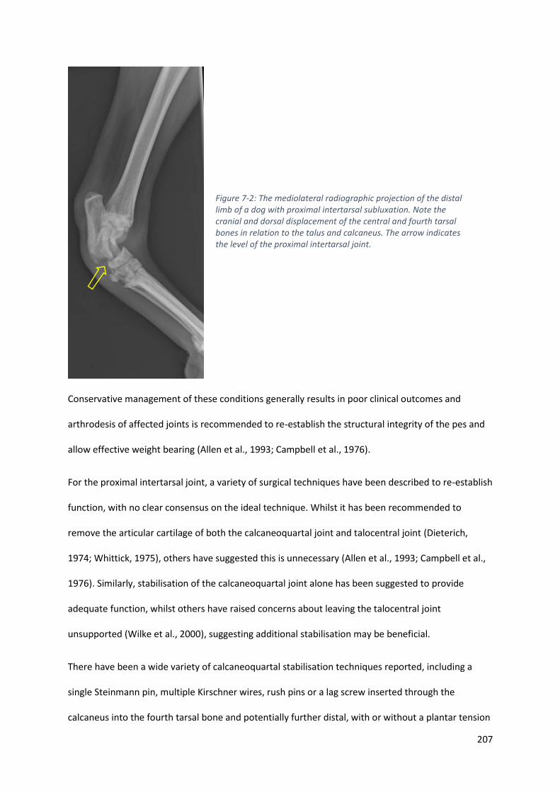
207

Conservative management of these conditions generally results in poor clinical outcomes and

arthrodesis of affected joints is recommended to re-establish the structural integrity of the pes and

allow effective weight bearing (Allen et al., 1993; Campbell et al., 1976).

For the proximal intertarsal joint, a variety of surgical techniques have been described to re-establish

function, with no clear consensus on the ideal technique. Whilst it has been recommended to

remove the articular cartilage of both the calcaneoquartal joint and talocentral joint (Dieterich,

1974; Whittick, 1975), others have suggested this is unnecessary (Allen et al., 1993; Campbell et al.,

1976). Similarly, stabilisation of the calcaneoquartal joint alone has been suggested to provide

adequate function, whilst others have raised concerns about leaving the talocentral joint

unsupported (Wilke et al., 2000), suggesting additional stabilisation may be beneficial.

There have been a wide variety of calcaneoquartal stabilisation techniques reported, including a

single Steinmann pin, multiple Kirschner wires, rush pins or a lag screw inserted through the

calcaneus into the fourth tarsal bone and potentially further distal, with or without a plantar tension

Figure 7-2: The mediolateral radiographic projection of the distal limb of a dog with proximal intertarsal subluxation. Note the cranial and dorsal displacement of the central and fourth tarsal bones in relation to the talus and calcaneus. The arrow indicates the level of the proximal intertarsal joint.

208

band wire. (Allen et al., 1993; Campbell et al., 1976; Dieterich, 1974). Other reported techniques

include ventral plating (Wilke et al., 2000), lateral plating(Campbell et al., 1976; Fettig et al., 2002)

extending from calcaneus to metatarsals, external skeletal fixation and pins and cast (Campbell et

al., 1976). Complication rates of 41-47% (Allen et al., 1993; Barnes et al., 2013) suggest that the

optimal fixation technique has not been established, however, a recent study regarding

complications following calcaneoquartal arthrodesis suggested lateral plate fixation was associated

with few complications when compared to pin and tension band wire techniques and was suggested

as the favoured technique (Barnes et al., 2013). A variety of plates have been used for this

procedure, including dynamic compression plates, hybrid plates, cuttable plates and limited contact

plates (Fettig et al., 2002; Scrimgeour et al., 2012; Théoret and Moens, 2007). Currently, there is no

data available comparing the performance of the different plates and the ideal configuration of the

construct, regarding screw numbers and the bones which they should engage.

To determine if lateral plating that engages the calcaneus, fourth tarsal bone and metatarsals could

adequately re-establish force transmission through the pes, a lateral plate repair in 10 canine

cadaveric limbs was performed. These limbs had all previously undergone complete transection of

the plantar ligament, which had resulted in a proximal intertarsal luxation. The experimental

hypothesis was that stabilisation of the calcaneoquartal joint would restore the integrity of the pes,

allowing force transmission comparable to the intact limb. The aim was to characterise the motion

of the individual tarsal bones after lateral plate repair of a proximal intertarsal luxation and compare

these motions to the intact limb when the same load was applied to the limbs.

209

7.2 Materials and methods

7.2.1 Specimens

Ten paired hind limbs (from 5 dogs) were used for this study. Briefly, these limbs were all obtained

from skeletally mature greyhounds, euthanised for reasons unrelated to this study. Limbs were

disarticulated and wrapped in cloth moistened with saline to prevent tissue dehydration and frozen

at-200C until testing. 24 hours prior to testing, limbs were thawed within a 40C refrigerator.

7.2.2 Limb loading

All limbs were prepared as previously described and loaded into a custom loading jig (as described in

chapter 4). Prior to testing, the stifle and tarsal joints were manually flexed and extended and then

preconditioned in the jig to a force of 600N, measured on the pressure sensitive film positioned

under the paw (Film code 5076-350. Tekscan, South Boston, MA, USA ), over five cycles (as described

in Chapter 5).

7.2.3 Study design

The overview of the study design is shown in figure 7.3. Briefly, each limb underwent CT scanning

when intact (in an unloaded position and following application of a 600N load) and again after

complete plantar ligament transection and repair with lateral bone plate and screws (in an unloaded

position and following application of a 600N load).

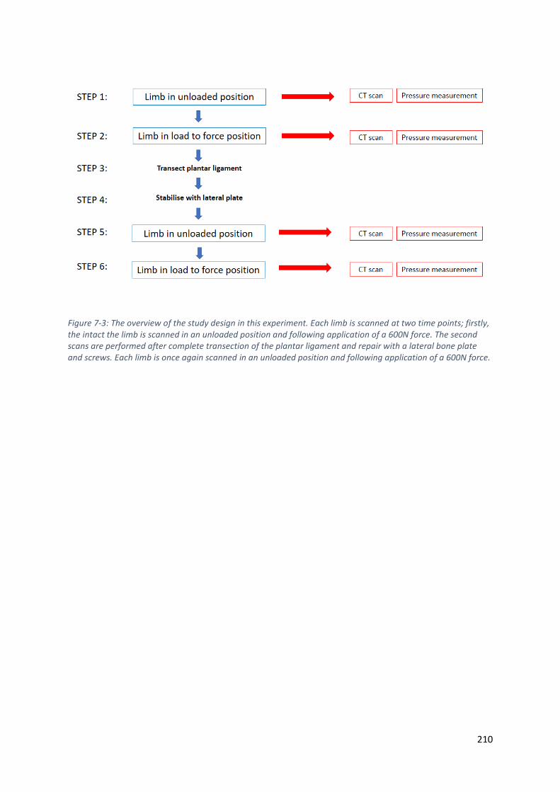
210

Figure 7-3: The overview of the study design in this experiment. Each limb is scanned at two time points; firstly, the intact the limb is scanned in an unloaded position and following application of a 600N force. The second scans are performed after complete transection of the plantar ligament and repair with a lateral bone plate and screws. Each limb is once again scanned in an unloaded position and following application of a 600N force.

211

7.2.4 Computed tomography scanning of the intact limb

All limbs had been used in the previous experiment and had undergone a CT scan (Philips Brilliance

16-slice CT scanner. Scanning parameters: 120KVP, 117 mA, slice thickness 1mm, slice increment

0.5mm, 512 X512 matrix) in an unloaded position and following application of a 600N load in the

custom designed limb loading jig.

The distance from the proximal limb restraint to the foot plate, termed linear displacement (figure

7.4) was recorded for the unloaded position and the load to force (600N) position. The motion of the

tibia, tarsal and metatarsal bones were calculated relative to the reference bone, the talus (as

previously described in chapters 3 and 4). Motions were recorded both as a series of 3 translations

and 3 rotations and as a total rotation about a single helical axis.

Figure 7-4: The limb in the custom designed limb loading jig. The linear displacement (red arrow) was the distance measured from the disc of the proximal limb restraint (A) to the top of the foot plate (B). Measurements were made with a measuring tape as shown in the image.

212

7.2.5 Ligament transection

All limbs then underwent complete transection of the plantar ligament, comprising the long plantar

ligament and the calcaneocentral ligament using a scalpel blade (as described in chapter 6).

Complete luxation of the proximal intertarsal joint was observed in all specimens following

application of a load (figure 6.8).

7.2.6 Surgical repair with laterally applied bone plate

The limbs were then removed from the limb loading jig and a 2.7mm titanium locking compression

plate (DePuy Synthes, Paoli, PA) was applied to the lateral aspect of the calcaneus, fourth tarsal

bone and metatarsals. Prior to application, the lateral aspect of the calcaneoquartal and

tarsometatarsal joint capsules were removed with a scalpel blade and a high-speed burr was used to

remove the head of MTV, creating a relatively flat surface over the lateral aspect of the pes. If

required, the plate was contoured to ensure maximal contact between the plate and the underlying

bone using bending irons (DePuy Synthes, Paoli, PA). A 2mm drill bit attached to a high-speed drill

(Ryobi, Fuchu, Hiroshima Prefecture, Japan) was used to create bone tunnels for the insertion of

2.7mm titanium self-tapping screws (DePuy Synthes, Paoli, PA). A 2.7mm universal drill guide (DePuy

Synthes, Paoli, PA) was used to position the holes in the neutral position of the combi-holes. 4

screws were placed in the calcaneus, 2 in the fourth tarsal bone and 4 in the metatarsals (figure 7.5).

The most proximal 2 screws in the metatarsals were inserted with the aim to engage either 3 or 4

metatarsals, whilst the distal most two were inserted to engage only MTV. There was no

standardisation of insertional torque of the screws, but each were inserted by an experienced

surgeon to a point that was considered appropriate for application of a bone plate. Screw length was

213

determined using a depth gauge with the aim of engaging only calcaneus and fourth tarsal bones

proximally. Articular cartilage was not removed in any case.

7.2.7 Computed tomography scanning of the repaired limb

Following bone plate application, each limb was repositioned in the limb loading jig using the same

proximal trans-tibial bone tunnel and scanned once again in an unloaded position and the linear

displacement recorded. The protocol for the CT scan remained identical to the previous scans

(Scanning parameters: 120KVP, 117 mA, slice thickness 1mm, slice increment 0.5mm, 512 X512

matrix)

Figure 7-5: The 2.7mm titanium locking compression plate applied to the lateral aspect of the pes. The site of plantar ligament transection (red arrow) marks the proximal intertarsal joint. The four most proximal screws are placed in the calcaneus, the central 2 screws (black arrows) are positioned within the 4th tarsal bones, whilst the distal 4 screws engage metatarsal bones.

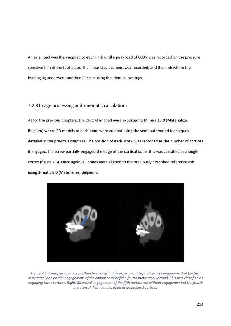
214

An axial load was then applied to each limb until a peak load of 600N was recorded on the pressure

sensitive film of the foot plate. The linear displacement was recorded, and the limb within the

loading jig underwent another CT scan using the identical settings.

7.2.8 Image processing and kinematic calculations

As for the previous chapters, the DICOM imaged were exported to Mimics 17.0 (Materialize,

Belgium) where 3D models of each bone were created using the semi-automated techniques

detailed in the previous chapters. The position of each screw was recorded as the number of cortices

it engaged. If a screw partially engaged the edge of the cortical bone, this was classified as a single

cortex (figure 7.6). Once again, all bones were aligned to the previously described reference axis

using 3-matic 8.0 (Materialize, Belgium).

Figure 7-6: Examples of screw position from dogs in this experiment. Left: Bicortical engagement of the fifth metatarsal and partial engagement of the caudal cortex of the fourth metatarsal (arrow). This was classified as engaging three cortices. Right: Bicortical engagement of the fifth metatarsal without engagement of the fourth

metatarsal. This was classified as engaging 2 cortices.

215

The motion of the tibia, tarsal and metatarsal bones were calculated relative the talus (reference

bone) and the total rotation and helical axis were calculated as described in the previous chapters.

Kinematic coupling between the previously identified rigid functional units (Central tarsal

bone/fourth tarsal bone, MTII/MTIII and MTIV/MTV), pairs of bones that cross the proximal

intertarsal joint (calcaneus/central tarsal bone and calcaneus/fourth tarsal bone) and pairs of bones

that were attached to the bone plate (calcaneus/fourth tarsal bone, calcaneus/ MTV and fourth

tarsal bone/MTV) was examined. For each pair, the co-efficient of variation, coupling ratio and

alignment angle was calculated as previously described.

7.2.9 Statistics

A two-tailed paired t-test was used to compare the linear displacement of the intact limb and the

repaired limb when a force of 600N was recorded on the force plate using Excel (Microsoft,

Redmond, Washington, USA). p < 0.05 was considered significant.

The total rotation for each individual bone was compared between intact and repaired conditions

using a two-tailed paired t-test with Excel (Microsoft, Redmond, Washington, USA). p < 0.05

considered significant.

216

7.3 Results

All limbs had 4 screws placed in the calcaneus and none of these screws engaged any aspect of the

talus. All limbs had 2 screws placed in the fourth tarsal bone and although some of the bone tunnels

entered the central tarsal bone, none of the screws engaged the central tarsal bone. There was

greater variability in the position of the 4 metatarsal screws. The two most proximal metatarsal

screws engaged a median of 6 cortices each (range 3-7), whilst the two distal metatarsal screws

engaged a median of 3 cortices (range 2-3) (table 7.1)

Table 7-1: The number of cortices engaged by each screw in all specimens. Screws are numbered from proximal to distal. None of the calcaneal screws (numbers 1-4) engaged the talus and similarly none of the fourth tarsal bone screws (numbers 5-6) engaged the central tarsal bone or third tarsal bones. There was more variability within the metatarsal screws (numbers 7-10) in terms of the number of cortices engaged. L = left limb, R = right limb.

The linear displacement and pressure on the foot plate was recorded for the intact and repaired

limbs in both then unloaded and loaded position (table 7.2). There was no difference in linear

displacement between the intact and repaired limbs when a load of 600N was recorded on the foot

plate. (p = 0.94)

1L 1R 2L 2R 3L 3R 4L 4R 5L 5R

1 2 2 2 2 2 2 2 2 2 2

2 2 2 2 2 2 2 2 2 2 2

3 2 2 2 2 2 2 2 2 2 2

4 2 2 2 2 2 2 2 2 2 2

5 2 2 2 2 2 2 2 2 2 2

6 2 2 2 2 2 2 2 2 2 2

7 6 6 6 6 6 6 5 6 6 7

8 6 3 6 7 7 3 6 3 6 3

9 3 3 3 3 3 3 3 2 3 2

10 3 3 3 3 3 2 2 2 2 2

calcaneus

fourth

tarsal bone

metatarsals

dog number (side)screw

numberbone

217

Table 7-2: The force and linear displacement for each limb recorded during the unloaded and loaded scans before transection and after lateral plate repair of a proximal intertarsal luxation. L = left, R = right, st dev = standard deviation.

For the intact limb, all tarsal and metatarsal bones underwent motion relative to the talus following

application of a 600N load (table 7.3). Similarly, all tarsal and metatarsal bones underwent motion

relative to the talus after the same load was applied to the repaired limbs (table 7.4).

Table 7-3: The 3 rotations and 3 translations of each bone recorded after application of a 600N load to the intact limb in the loading jig. The total (summative) rotation of each bone is also reported. CTB = central tarsal bone, TB = tarsal bone, MT = metatarsal bone, SD = standard deviation.

force (N)

linear

displacement

(cm)

force (N)

linear

displacement

(cm)

force (N)

linear

displacement

(cm)

force (N)

linear

displacement

(cm)

1 L 150.0 34.5 600.0 31.0 112.0 36.0 600.0 33.5

1 R 94.0 35.0 600.0 32.0 110.0 36.0 600.0 33.0

2 L 100.0 35.8 600.0 32.3 54.0 37.6 600.0 32.5

2 R 70.0 36.6 600.0 32.5 64.0 37.7 600.0 32.6

3 L 33.0 35.9 600.0 30.4 34.0 35.8 600.0 30.4

3 R 34.0 35.5 600.0 31.2 35.0 36.5 600.0 31.3

4 L 25.0 38.0 600.0 34.7 64.0 38.3 600.0 34.3

4 R 20.0 38.0 600.0 34.5 50.0 38.7 600.0 33.9

5 L 29.0 38.9 600.0 34.3 34.0 38.9 600.0 33.0

5 R 34.0 38.9 600.0 34.9 30.0 38.9 600.0 33.0

58.9 36.7 600.0 32.8 58.7 37.4 600.0 32.8

43.2 1.6 0.0 1.7 30.2 1.3 0.0 1.2

mean

st dev

sidedog

unloaded

Intact limb

load to 600N

Repaired limb

unloaded load to 600N

x axis y axis z axis x axis y axis z axis

mean 19.98 1.66 10.47 0.72 -15.62 1.52 15.75

SD 5.13 1.66 1.69 1.08 2.01 0.77 1.98

mean 0.21 0.24 0.08 -1.37 1.13 -0.40 1.86

SD 0.13 0.07 0.08 0.80 0.72 0.25 1.07

mean 0.15 0.39 0.54 -1.35 2.18 -0.40 2.66

SD 0.09 0.13 0.21 0.64 1.01 0.26 1.09

mean 0.22 0.62 1.03 -1.50 2.55 -0.83 3.13

SD 0.13 0.19 0.42 0.59 1.17 0.19 1.18

mean 0.14 0.64 1.14 -0.89 3.25 -0.80 3.53

SD 0.09 0.19 0.43 0.63 1.19 0.26 1.19

mean 0.22 0.63 0.98 -0.89 3.74 -1.05 4.14

SD 0.10 0.19 0.40 0.70 1.57 0.76 1.47

mean 0.28 1.72 4.48 0.45 5.45 -1.37 5.66

SD 0.13 0.42 1.31 0.47 1.48 0.39 1.46

mean -0.17 1.71 5.30 0.55 5.94 -1.10 6.12

SD 0.10 0.45 1.60 0.66 1.60 0.41 1.53

mean -0.23 1.84 5.36 -1.47 6.13 -1.58 6.63

SD 0.11 0.47 1.70 1.30 1.63 0.47 1.74

mean 0.05 1.87 5.37 -1.39 6.08 -1.48 6.55

SD 0.10 0.50 1.66 1.45 1.54 0.46 1.74

MT III

MT IV

MT V

Calcaneus

CTB

Fourth TB

Third TB

Second TB

MT II

translation along (mm) rotation around (degrees) total rotation

(degrees)

Tibia

All limbs: Load to force (600N) for

intact limbs

218

Table 7-4: The 3 rotations and 3 translations of each bone recorded after application of a 600N load to the repaired limb in the loading jig. The total (summative) rotation of each bone is also reported. CTB = central tarsal bone, TB = tarsal bone, MT = metatarsal bone, SD = standard deviation.

The calcaneus (p = 0.049) showed a significantly increase in total rotation in the repaired limb

compared to the intact limb, whilst both MTIV (p =0.001) and MTV (p=0.0001) both showed

significantly less total rotation in the repaired limb compared to the intact limb.

All other bones showed no significant different between repaired and intact limbs. However, the CTB

(p = 0.067) showed a trend towards a significant increase in total rotation between repaired and

intact limbs, whilst the MTIII (p = 0.055) showed a trend towards a significant decrease in total

rotation between repaired and intact limbs (figure 7.7).

x axis y axis z axis x axis y axis z axis

mean 23.17 2.30 12.62 1.20 -18.11 1.90 18.30

SD 6.88 2.48 2.41 1.59 3.25 1.11 3.28

mean 0.24 0.34 0.27 -2.01 0.63 -0.94 2.70

SD 0.16 0.13 0.16 0.48 1.48 0.83 0.93

mean 0.06 0.69 0.85 -1.25 3.02 -0.42 3.59

SD 0.15 0.30 0.36 0.98 1.66 1.05 1.62

mean 0.18 0.94 1.40 -0.78 2.99 -0.87 3.52

SD 0.20 0.48 0.70 1.07 1.60 0.85 1.49

mean 0.02 0.92 1.52 -0.98 3.69 -0.87 4.16

SD 0.18 0.47 0.65 1.05 1.69 0.92 1.67

mean 0.02 0.90 1.20 -2.76 2.78 0.30 5.68

SD 0.32 0.47 0.71 7.25 2.10 1.77 6.45

mean 0.02 2.04 4.47 0.21 4.50 -1.65 5.09

SD 0.33 1.10 1.88 0.88 1.97 0.91 1.89

mean -0.41 1.85 5.04 0.66 4.70 -1.02 4.97

SD 0.41 1.08 2.27 1.02 2.15 0.79 1.89

mean -0.21 1.68 4.62 -0.10 4.07 -0.77 4.44

SD 0.35 1.06 2.33 1.07 1.97 0.77 1.68

mean 0.20 1.57 4.27 0.53 3.67 -0.54 4.10

SD 0.27 1.11 2.30 1.22 1.79 0.69 1.45

Second TB

MT II

MT III

MT IV

translation along (mm) rotation around (degrees) total rotation

around helical axis

(degrees)

All limbs: Following lateral plate

repair

MT V

Tibia

Calcaneus

CTB

Fourth TB

Third TB

219

Figure 7-7: The total rotation of each bone for the intact limb and the repaired limb. Lateral plate repair reduced rotation in all metatarsal bones, but significantly for the two lateral digits, which were closest to the plate. No significant difference in rotation was seen in all other tarsal bones. CTB = central tarsal bone. TB = tarsal bone, MT = metatarsal bone.

* denotes a significant difference between intact and repaired conditions for that bone. Error bars are one standard deviation

The kinematic coupling of the bones that cross the proximal intertarsal joint was not restored

following application of a lateral bone plate. The angle between the helical axis of both bones

(alignment angle) was similarly not restored after plate repair (table 7.5).

In contrast, the kinematic coupling of the previously identified functional units remained high after

repair. However, the alignment angle increased significantly in all pairs following plate repair,

demonstrating that their rotations became more divergent after plate repair (table 7.5).

For the bones that were attached to the lateral bone plate, there was an increase in kinematic

coupling of these pairs with the exception of the calcaneus/fourth tarsal bone pairing. However, the

*

* *

220

rotation of these pairs was not around a similarly orientated as demonstrated by the large alignment

angle values.

Table 7-5: The correlation coefficient, coupling ratio and alignment angle for pairs of tarsal or metatarsal bones. The top rows are pairs of bones that cross the proximal intertarsal joint. The middle, shaded rows and the previously identified rigid functional units, whilst the bottom shaded pairs are pairs that are attached to the bone plate. There was a loss of coupling (decreased correlation co-efficient) for bones across the proximal intertarsal joint following repair and a significant difference in alignment angle for most pairs of bones.

* denotes significant difference between intact limb and repaired limb. CTB= central tarsal bone, 4th = fourth tarsal bone, MT = metatarsal

correlation

coefficient

(R2)

coupling

ratio

alignment

angle of

helical axes

(degrees)

correlation

coefficient

(R2)

coupling

ratio

alignment

angle of

helical axes

(degrees)

Calcaneus and CTB 0.92 0.97 20.1 ± 8.0 0.34 1.02 44.1 ± 14.6*

Calcaneus and 4th 0.94 1.07 20.3 ± 11.6 0.54 1.18 57.0 ± 29.5*

CTB and 4th 0.93 1.04 9.6 ± 5.5 0.92 0.88 16.6 ± 7.4*

MTII and MTIII 0.98 1.04 4.8 ± 2.6 0.98 0.99 13.1 ± 6.4*

MTIV and MTV 0.97 0.98 2.7 ± 2.4 0.87 0.81 13.1 ± 11.3*

Calcaneus and 4th 0.94 1.07 20.3 ± 11.6 0.54 1.18 57.0 ± 29.5*

Calcaneus and MTV 0.66 1.32 40.2 ± 15.2 0.76 1.36 78.4 ± 29.9*

4th tarsal and MTV 0.80 1.32 20.5 ± 8.9 0.90 0.92 22.4 ± 10.6

Pair of bones

Intact limb Following repair

221

7.4 Discussion

The findings of this study demonstrate that the application of a lateral bone plate to the calcaneus,

fourth tarsal bone and metatarsals is able to re-establish force transmission through the pes

following proximal intertarsal luxation. It suggests that stabilisation of the medial column (the talus,

central tarsal bone, third tarsal and third metatarsal) is not required to allow the pes to act

effectively as a lever in the distal limb, providing additional data that may help resolve the open

question of what is the most appropriate surgical technique to treat proximal intertarsal subluxation

in the dog.

In the canine limb, there is no substantial ligamentous connection between the plantar aspect of the

talus and central tarsal bone. Rather, the plantar support for the central tarsal bone, runs from its

plantar process to the large medial projection of the calcaneus, the sustentaculum tali. (Evans et al.,

2012). This arrangement allows the tensile force on the tuber calcanei to be transferred to both the

medial and lateral aspect of the pes through the central and fourth tarsal bone respectively

(Arwedsson, 1954). By stabilising the fourth tarsal bone with the calcaneus, the central tarsal bone

motion is limited indirectly through its tight coupling with the fourth tarsal bone, which was

demonstrated in chapter 5. This finding is also in agreement with the work in chapter 6, where

transection of the calcaneocentral ligament resulted in only mild increases in central tarsal bone

motion due to its strong attachment to the fourth tarsal bone.

Configuration of surgical stabilisation

In clinical practice, a major question that remains unresolved is what is the optimal surgical

technique to re-establish force transmission through the pes following proximal intertarsal luxation.

Numerous different implants and configurations of implants have been reported in the treatment of

clinical cases (Allen et al., 1993; Campbell et al., 1976; Fettig et al., 2002; Roch et al., 2008;

222

Scrimgeour et al., 2012; Wilke et al., 2000) with a retrospective comparison of techniques reporting

fewer complications with lateral plating compared to pin or screw and tension band (Barnes et al.,

2013). However, a comparison of techniques should ensure that there is standardisation of implant

configuration within techniques as this may influence biomechanical performance and clinical

outcome. For example, in cases of pin and screw fixation (with or without a tension band) there is

variable extension of the pin or screw into the metatarsal bones in reported case series (Allen et al.,

1993; Barnes et al., 2013; Scrimgeour et al., 2012). Although implants crossing the tarsometatarsal

joints may influence the stability of the repair by immobilising the tarsometatarsal joint in addition

to the calcaneoquartal joint, the effect of placing implants across the tarsometatarsal joint is yet to

be evaluated as a factor which may influence the incidence of complications, biomechanical

performance and clinical outcome. Additionally, it is important to consider complications related to

inappropriate application of fixation techniques. In the study of Barnes et al. 2013, there were cases

of pin and tension band wire application to comminuted fractures, which is an example of

inappropriate case selection and may influence complication rates.

In contrast to pin and screw-based repairs, all published reports of plate stabilisation across the

proximal intertarsal joint span the tarsometatarsal joints to include the metatarsal bones. However,

within plated repairs, there is little standardisation with a number of different plate designs used

with varying screw configurations (Barnes et al., 2013; Fettig et al., 2002; Roch et al., 2008;

Scrimgeour et al., 2012; Théoret and Moens, 2007).

The pes experiences large bending moments during loading (Alexander, 1974; Alexander, 1984) and

surgical repair of proximal intertarsal subluxations must counteract these moments until complete

bony union is achieved. Implant failure is a common complication of repair due to high magnitudes

of repetitive loads. A laterally positioned bone plate is loaded on edge, towards its greatest

dimension (Dyce et al., 1998). This substantially increases its moment of inertia, which resists the

bending moment. The 2.7mm plate used in this experiment has a width of 7.5mm and a thickness of

223

2.6mm, producing a secondary area moment of inertia (AMI) of 91.4mm4 when loaded on edge

(compared to an AMI of 10.99mm4 if loaded towards its narrowest dimension). This particular plate

was selected as it allowed appropriate screw size selection in the metatarsal bones and allowed two

screws to be positioned in the fourth tarsal bone. Although a larger 3.5mm plate would have further

increased the secondary AMI, it would result in the metatarsal screws exceeding the recommend

bone:screw diameter (Johnson et al., 2005). A hybrid plate which accepts different size screws in the

proximal and distal fragments would have been a suitable alternative and has been used successfully

in clinical cases (Fettig et al., 2002), however, this plate is currently only available in stainless steel.

Newly developed intertarsal arthrodesis plates are also available and have been developed with

appropriate lengths for engaging the calcaneus and metatarsals. Previous experience with stainless

steel plates revealed increased CT artefacts compared to titanium plates, due to the higher x-ray

attenuation coefficient of steel (Lee et al., 2007). Titanium plates were selected in preference to

316L stainless steel as the use of stainless steel plates may have prevented accurate segmentation of

each individual tarsal bone. As a surface matching algorithm (Besl and McKay, 1992) was used to

calculate the motion of each bone, accurate segmentation is critical to produce accurate kinematic

results (Tan et al., 2017).

One important consideration when interpreting these findings is the differing material properties of

titanium and stainless steel. The modulus of elasticity of titanium is approximately half that of steel,

resulting in twice as much deformation for the same applied load (Niinomi, 1998). During testing, no

obvious visual deformation of the titanium plates was observed, however, small motions were

identified between the bones that were attached to the plate suggesting some deformation of the

plate had occurred or alternatively, some motion occurred between the screws and the plate. This

means that the reported motions include any contribution made due to deformation of the plate or

motion between the screw heads and the plate. As all limbs were of similar size and all plates and

screws were of the identical material and dimensions, the variation across specimens was

224

minimised. However, these results cannot be directly translated to surgical repairs performed with

316L stainless steel plates or plates of different size or design.

There is an opportunity to engage the central tarsal bone and third tarsal bone by placing longer

screws through the fourth tarsal bone (Dyce et al., 1998; Fettig et al., 2002). In doing so, these

screws may further help stabilise the central tarsal bone in relation to the calcaneus. However, there

is also a potential risk of screw loosening when placed across a low motion joint, as the repeated

motion may “toggle” the screw loose. Of 58 calcaneoquartal arthrodeses performed using laterally

applied plates, 5 cases required screw removal due to loosening. Four of the five cases involved the

screw in the fourth tarsal bone, whilst the remaining loose screw was positioned across multiple

metatarsal bones (Barnes et al., 2013). It was not reported whether or not these screws also

engaged the central or third tarsal bones. Loosening appears to be the more common mode of

failure of the screw in the fourth tarsal bone as bending or breakage of this screw was not reported

(Barnes et al., 2013) During triple pelvis osteotomy procedures, cortical screws that penetrated

through the ilium and crossed the low motion sacro-iliac joint before engaging the sacrum were

shown to have an increased likelihood of loosening when compared to screws that did not cross the

joint (Doornink et al., 2006). Future studies may choose to include this additional variable of central

tarsal bone engagement to identify if this provides additional stability to the construct. However, to

determine its effect on construct longevity, a cyclic loading model would be recommended.

The results of this chapter suggest that central tarsal bone engagement may not be required since

force transmission was restored with engagement of the fourth tarsal bone alone. The force applied

to cadaveric limbs in this study (600N) represents approximately 1.6 times the body weight for an

adult greyhound, which is the maximum recorded load for a galloping dog (Walter and Carrier, 2007;

Walter and Carrier, 2009). This is likely to exceed the maximal force applied to limb in the post-

operative recovery period, when exercise restriction is recommended (Roch et al., 2008). If force

transmission can be restored through redirection of tensile forces through alternate ligamentous

225

pathways for these magnitudes, then gaining additional rigidity through central tarsal bone

engagement may not be required, however, cyclic testing would be required to verify this

assumption.

The decision not to engage the central tarsal bone would also be based on the assumption that the

ligamentous support between the central and fourth tarsal bones remains intact. Based on the

preoperative radiographs, it may be beneficial to engage the central tarsal bone if there is any

suggestion of ligament failure between the central and fourth tarsal bones, as demonstrated by an

alteration in the joint space.

Depending on the hole spacing in the selected plate, it may not be possible to achieve the placement

of two screws in the fourth tarsal bone, and hence achieve rotational stability, making engagement

of the metatarsals more desirable. The 2.7mm plate used in this study allowed for the safe

placement of two screws in the fourth tarsal bone providing rotational stability. However, this

configuration of two non-locking cortical screws would not provide adequate fixation for clinical use

based upon current AO principles of fixation, which suggest a minimum of 6 cortices in each

fragment (Johnson et al., 2005). For this reason, the length of plate was selected to allow for

engagement of the metatarsal bones.

From the data in this chapter, it is therefore not possible to draw conclusions about restoring force

transmission by stabilisation of the calcaneoquartal joint alone (as the tarsometatarsal joints were

included in the surgical repair. Indeed, if this was possible in a clinical setting, preservation of motion

at the tarsometatarsal joints may have additional benefits in preserving the natural elasticity of the

pes, allowing for energy absorption following the impact of the paw on the ground and storage of

elastic strain energy throughout the stance phase of gait. Alternatively, the increased lever arm

created by a fused calcaneus and fourth tarsal bone may place additional strain on the

tarsometatarsal joint, leading to injury or premature degeneration, however, this has not been

226

reported when a pin and tension band wire alone was used to stabilise the calcaneoquartal joint in

isolation (Allen et al., 1993; Barnes et al., 2013; Campbell et al., 1976)

The evolution of locking bone plates in recent years, may in fact, allow adequate plate stabilisation

of the calcaneoquartal joint without involvement of the tarsometatarsal joints. These plates, in

which the screw heads rigidly engage the plate hole, create an angle stable construct that does not

rely upon compression of the plate to the underlying bone for stability (Egol et al., 2004; Niemeyer

and Sudkamp, 2006; Wagner, 2003). It has been suggested that two screws in each bone fragment

produces adequate stability (Niemeyer and Sudkamp, 2006) and this may allow for adequate

stabilisation of the fourth tarsal bone with the calcaneus. The use of these plates in treatment of

proximal intertarsal instability warrants further investigation and particularly, the effect of

preserving the tarsometatarsal joints.

The clinical outcome following calcaneoquartal arthrodesis as generally reported to be good based

upon owner assessment and this is commonly attributed to the low magnitude of motion that

normally exists at this joint (Allen et al., 1993; Fettig et al., 2002). However, only 50% of working

dogs could return to full activity following partial tarsal arthrodesis (Scrimgeour et al., 2012) and

significant asymmetry was identified in the only study of calcaneoquartal arthrodesis that utilised

objective force plate data, despite no clinically detectable lameness (Wilke et al., 2000). One possible

cause for the poorer outcomes may be disruption of the elastic dorsiflexion mechanism of the pes,

which cushions impact and conserves energy (Alexander, 1984). This disruption may be unavoidable

during repair of proximal intertarsal subluxation but must be a consideration when providing owners

with a prognosis following surgical repair.

Another possible cause for ongoing lameness may be due to the immobilisation of neighbouring

joints and subsequent ankylosis, which has been observed in joints that have not been debrided

(Campbell et al., 1976; McLennan, 2007). Ankylosis, the pathological fusion of a joint, may be

responsible for ongoing morbidity and is the likely fate of the tarsometatarsal joints when a lateral

227

plate engages the metatarsal bones. This may further support the investigation of calcaneoquartal

stabilisation without metatarsal involvement. It is unclear from the literature, if debriding multiple

joint spaces results in a more stable pes and ultimately improved clinical function.

In the previous chapter, the helical axis of the fourth and central tarsal bones were identified and

were located remote to each bone in all cases. This means that translation of the central and fourth

tarsal bones occurs at the articular surface. It is unclear if the motion of these bones would differ if

articular cartilage debridement was performed prior to plate application. The effect of packing with

cancellous bone graft and producing interfragmentary compression, as would be performed

clinically, also remains unknown and care must be taken when extrapolating these findings to the

clinical setting (Barnes et al., 2013; Roch et al., 2008). Articular debridement was not performed in

this experiment to prevent the introduction of additional variables including the degree of

debridement of each surface and total volume, fragment size and porosity of any autogenous

cancellous bone graft.

The effect of lateral plate repair of a proximal intertarsal luxation had significant effects on the

highly coupled and co-ordinated motions of the tarsal and metatarsal bones. Plate repair could not

restore the normal kinematic coupling across the proximal intertarsal joint, as reported in chapter 5,

and this likely reflects the different material properties of the plate compared to the plantar

ligament and the different location and pattern of loading. The plate was also seen to alter the

helical axis of the previously identified functional units. Although the correlation co-efficient

remained high for these pairs, the redirection of force through the plate (rather than the plantar

ligament) altered the orientation of their helical axis. This once again demonstrates the reliance of

each tarsal bone on the motion of neighbouring bones for both its magnitude and orientation of

rotation (Sennwald et al., 1993). Interestingly, even bones rigidly attached to the bone plate did not

share a common axis of rotation as may be expected if they were to function as a single unit.

Deformation of the plate during loading is one possible explanation and this may not simply occur in

228

the sagittal plane. The lateral plate is eccentrically located on the pes and during loading it is likely to

have to counter both dorsiflexion of the pes and rotation of the pes. The oblique helical axis

identified for MTV suggests that the plate may have deformed by torsion. The previous experiments

of this thesis identified that internal rotation and dorsiflexion occur concurrently during limb loading

and this would have exposed the plate to both on edge and rotational forces. The effect of this

degree of deformation on the progression of bony fusion across an arthrodesis site is beyond the

scope of this chapter but future studies may investigate if plate size, design and screw purchase may

influence the degree of individual tarsal and metatarsal bone motion after limb loading.

A decrease in the correlation coefficient of the calcaneus and fourth tarsal bone was also observed

following plate application. This finding may be somewhat surprising given that both bones are now

attached to the plate, however, it may reflect the interdependent nature of intertarsal bone motion

whereby fusion of one joint may affect the kinematics of the adjacent joints (Astion et al., 1997).

Limitations

This study has a number of limitations that must be acknowledged for the contribution they may

have made to the overall results. Firstly, the majority of proximal intertarsal luxations present with

evidence of remodelling changes consistent with their insidious onset (Campbell et al., 1976). These

changes were not present in the normal limbs that were studied in this experiment. Sharp

transection of a normal plantar ligament is unlikely to accurately reflect the clinical presentation of

proximal intertarsal luxation. Periarticular osteophytosis and fibrosis may influence the kinematics of

individual tarsal bones and could not be replicated in our model of proximal intertarsal subluxation.

As discussed in previous chapters, the use of cadaveric limbs requires active replication of all

relevant muscle forces. The major forces on the tarsal bones can be replicated by this limb loading

jig, however, not all muscular forces, particularly those of the interosseous muscles on the pes, were

replicated and this fact must be considered when interpreting these results.

229

The lateral plate repair restored the integrity of the pes as the lever arm, which allows force to be

transmitted through the distal limb (Alexander, 1984). However, our loading was applied as a single,

non-destructive load that does not represent the repetitive loads that would be experienced by the

pes during the period until a bony union is achieved. It is unknown if the configuration used in this

experiment would provide adequate stability over time and therefore, the suggestion that

engagement of the fourth tarsal bone alone is adequate must be applied with caution. Future

studies may investigate the effect of plate configuration, including the number of screws used in

each bone and the number of bones that are engaged by each screw, on cyclic loading of the pes

repaired with a lateral plate.

The method of loading that was utilised in the present study, relies upon the integrity of the intact

gastrocnemius muscle and superficial digital flexor tendon. It is unknown if these structures would

survive cyclic testing and continue to produce the appropriate internal forces on the tarsal bones.

Previous limb loading jigs (Warzee et al., 2001) have replicated the pull of the gastrocnemius with a

wire and turnbuckle which may be one modification to our loading protocol that may support cyclic

fatigue testing. The proximal limb restrain could be easily reproduced to be compatible with the

attenuator of a sevohydraulic materials testing machine. This approach was not used in this

kinematic study as it was believed that the intact gastrocnemius insertion would most accurately

replicate the in vivo force on the tuber calcanei and was adequate for the small number of cycles

used in these experiments.

When comparing the absolute motion of bones, one critical factor is the starting position for each

bone. In the intact limb, it has been suggested that there is some free-play between bones when a

load is not applied. To minimise the chance of any free-play, it was ensured all limbs had a small

amount of force recorded on the foot plate, however, when ligaments are not taught, other forces,

such as gravity, will influence bone position.

230

The application of a non-locking bone plate would also alter the starting position of each bone, as

recorded in the unloaded scan as bones are pulled up towards the plate during screw tightening.

Accurate contouring of the plate will reduce this effect, but absolutely perfect contouring is

unrealistic in any clinical situation and will have subtle effects on bone position. Both plate

contouring and burring of the lateral head of MTV were carefully performed to minimise this effect.

A second unloaded scan was performed after repair and used as the start position for the loaded

repaired limb rather than using the position of each bone in the unloaded scan of the intact limb.

7.5 Conclusions

The findings outlined in this chapter have identified that, following complete plantar ligament

transection, application of a lateral bone plate and screws that engage the calcaneus, fourth tarsal

bone and metatarsals will contribute to the redirection of force through the pes, which allows it to

act effectively as a lever arm. Although, no assumptions can be made about maintaining stability

over time, the repaired pes could generate a ground reaction force that was no different to that

generated by the intact foot at similar displacements.

231

Chapter 8 : Thesis conclusions

232

The common practice of modelling the canine pes as a rigid limb segment, despite the well-

recognised ability to produce motion at the intertarsal joints during clinical examination, provided

one of the major motivations of this thesis. With no published descriptions of canine tarsal bone

kinematics, there is limited understanding regarding the nature of movement within the pes during

locomotion and how these motions may be implicated in fatigue fractures of the tarsal bones and

degeneration of the plantar ligament. Describing the nature of tarsal bone motion may also be an

important consideration when planning and evaluating surgical repairs of the canine pes.

Thus, the major aims of this thesis were i) to develop a technique to allow quantification of tarsal

bone kinematics based on computed tomography imaging (chapters 3 and 4) and ii) application of

this technique to normal cadaveric limbs (chapter 5), following sequential transection of the plantar

ligament (chapter 6) and following lateral plate stabilisation (chapter7). The most important

contributions of this thesis are summarised in the following paragraphs.

8.1 Major contributions

Chapter 3 detailed the computed tomography based kinematic techniques used throughout this

thesis, revealing that segmentation threshold, reconstruction algorithm and scan resolution did not

significantly influence kinematic accuracy. This means segmentation thresholds and reconstruction

algorithms can be set at the most convenient settings which may lead to improvements in the

efficiency of kinematic processing. Perhaps most significantly, was the finding that a reduction in

radiation exposure, achieved by decreasing scan resolution, will not reduce kinematic accuracy.

Although of little consequence in cadaveric investigations, this result may be of great importance in

in vivo studies using human patients. In this chapter, the techniques described were shown to be

highly accurate for identifying motion within canine tarsal bones, making them suitable for

application in the following chapters.

233

Chapter 4 reports the design features and principles behind development of a cadaveric limb loading

jig. Although the jig described in this chapter was optimised for loading of the pelvic limb of the dog,

many of the principles and features could also be applied to both the canine pectoral limb or limbs

of other species. Features such as the femoral block permit accurate replication of in vivo joint

angles and can be easily installed into any future loading jig. This jig could also be used in future

studies, investigating the effect of both ligament damage and fractures of the pes, whilst also

providing insights into how various repair techniques restore the normal pattern of bone motion.

Chapter 5 provides the first description of the motion that each individual tarsal bone undergoes

during weight bearing. The results reveal that although the majority of motion occurs at the

talocrural joint as has been previously described, the collective motion at the intertarsal and

tarsometatarsal joints contribute significantly (up to 28.9 %) to sagittal plane flexion. This

dorsiflexion of the pes may be a significant component to the “biological springs” of canine pelvic

limbs. Each bone demonstrated a unique helical axis, about which it rotates, with varying degrees of

obliquity to the anatomical reference planes. The direction and magnitude of these motions may be

applied to future investigations into the repetitive loading and potential fatigue failure of commonly

injured tarsal bones, such as the right central tarsal bone. From the results of this study, a simplified

model of the canine pes was proposed based on identification of rigid functional units within the

canine pes. This may simplify kinematic measurements in all future studies that acknowledge

intertarsal motion rather than modelling the pes as a single rigid segment.

Chapter 6 investigated the effect of partial plantar ligament transection on tarsal bone kinematics,

providing an insight into the role played by various components of the plantar ligament during

weight bearing. The results contribute to our understanding of the unanswered question of which

components of the plantar ligament are damaged to allow proximal intertarsal luxation, suggesting

that total loss of the plantar ligament is required to produce a proximal intertarsal luxation. The

strong ligamentous attachments between the talus and calcaneus, as well as the central and fourth

234

tarsal bones were responsible for maintaining the integrity of the pes despite partial transection of

the plantar ligament. These strong attachments would be further investigated in chapter 7.

Chapter 7 evaluated the effect of a lateral plate repair on tarsal bone kinematics and restoration of

the integrity of the pes following proximal intertarsal luxation. The results show that a bone plate

engaging the calcaneus, fourth tarsal bone and metatarsals was sufficient to restore force

transmission through the pes in static testing. This finding provides important new insights into the

configuration of laterally applied bone plates which can be applied in a variety of configurations.

Whilst some repairs utilise long screws to engage the central, third and second tarsal bones, the

results of this chapter suggest that it may be unnecessary and may even lead to premature

loosening, due to the observed motion between all tarsal bones, despite application of the bone

plate.

8.2 Future directions

Acknowledging the important contributions made by intertarsal bone motions is the first step to

revealing the true importance of the pes in animal locomotion. Validation of the kinematic results in

this thesis against in vivo studies will be an important step despite the technical challenges involved,

however, as biplanar fluoroscopy and 2D-3D matching techniques continue to evolve, it becomes

increasingly feasible. Once validated, the limb loading jig could be used to investigate other

anatomical structures within the pes and the effect of a variety of surgical interventions or repairs.

The capability to produce angulation of the foot plate and rotational forces within the limb will allow

a more complete evaluation of the limb in future studies.

Another interesting research possibility would be to compare of the kinematics of the pes in a

variety of species, such as the kangaroo or wallaby, which have previously been identified as animals

which have a high dependence on elastic energy stores in the distal limb.

235

The work presented in this thesis also suggests that future kinematic studies should consider

increasing the number of markers placed on the pes to better reflect the non-rigid nature of the pes.

The highly consistent contributions made by each joint suggest the pes could be modelled as a

three-segment model when viewed from the lateral aspect, comprising the calcaneus, the fourth

tarsal bone and the fifth metatarsal bone.

The computed tomography based kinematic techniques outlined in this thesis also have potential

applications in the clinical assessment of patients and evaluation of surgical interventions. CT scans

performed with and without an applied load or in 2 extremes of motion could be used to

characterise the normal range of motion in a variety of joints and may help in the diagnosis of

instability or ligament damage. Furthermore, scans performed before and after a surgical treatment

could be used to evaluate the success of the procedure.

236

References

Agostinho, F., Rahal, S. C., Miqueleto, N., Verdugo, M., Inamassu, L. and El-Warrak, A. (2011). Kinematic analysis of Labrador Retrievers and Rottweilers trotting on a treadmill. Veterinary and Comparative Orthopaedics and Traumatology 24, 185-191. Alexander, R. (1974). The mechanics of jumping by a dog (Canis familiaris). Journal of Zoology 173, 549-573. Alexander, R., Maloiy, G., Ker, R., Jayes, A. and Warui, C. (1982). The role of tendon elasticity in the locomotion of the camel (Camelus dromedarius). Journal of Zoology 198, 293-313. Alexander, R. and Vernon, A. (1975). The mechanics of hopping by kangaroos (Macropodidae). Journal of Zoology 177, 265-303. Alexander, R. M. (1984). Elastic energy stores in running vertebrates. American Zoologist 24, 85-94. Alexander, R. M. (2002). Tendon elasticity and muscle function. Comparative Biochemistry and Physiology Part A: Molecular & Integrative Physiology 133, 1001-1011. Alexander, R. M. (2005). Mechanics of animal movement. Current Biology 15, R616-R619. Alexander, R. M. and Bennet-Clark, H. (1977). Storage of elastic strain energy in muscle and other tissues. Nature 265, 114-117. Allen, M., Dyce, J. and Houlton, J. (1993). Calcaneoquartal arthrodesis in the dog. Journal of Small Animal Practice 34, 205-210. Anderson, F. C. and Pandy, M. G. (2001). Static and dynamic optimization solutions for gait are practically equivalent. Journal of Biomechanics 34, 153-161. Apelt, D., Kowaleski, M. P. and Boudrieau, R. J. (2007). Effect of tibial tuberosity advancement on cranial tibial subluxation in canine cranial cruciate‐deficient stifle joints: an in vitro experimental study. Veterinary Surgery 36, 170-177. Nussbaum, M. C. (1978). Aristotle's De motu animalium: text with translation, commentary, and interpretive essays. Princeton, N.J: Princeton University Press. Arndt, A., Wolf, P., Liu, A., Nester, C., Stacoff, A., Jones, R., Lundgren, P. and Lundberg, A. (2007). Intrinsic foot kinematics measured in vivo during the stance phase of slow running. Journal of Biomechanics 40, 2672-2678. Aron, D. N. and Purinton, P. T. (1985a). Collateral ligaments of the tarsocrural joint - an anatomic and functional-study. Veterinary Surgery 14, 173-177. Aron, D. N. and Purinton, P. T. (1985b). Replacement of the collateral ligaments of the canine tarsocrural joint - a proposed technique. Veterinary Surgery 14, 178-184. Arwedsson, G. (1954). Arthrodesis in traumatic plantar subluxation of the metatarsal bones of the dog. Journal of the American Veterinary Medical Association 124, 21. Astion, D. J., Deland, J. T., Otis, J. C. and Kenneally, S. (1997). Motion of the hindfoot after simulated arthrodesis. JBJS 79, 241-6. Attarian, D. E., McCrackin, H. J., DeVito, D. P., McElhaney, J. H. and Garrett Jr, W. E. (1985). Biomechanical characteristics of human ankle ligaments. Foot & ankle 6, 54-58. Aulakh, K. S., Harper, T., Lanz, O., D'Amico, L., Butler, J., McLaughlin, R. and Werre, S. (2013). Effect of tibial insertion site for lateral suture stabilization on the kinematics of the cranial cruciate ligament deficient-stifle during early, middle and late stance. Veterinary and Comparative Orthopaedics and Traumatology 26, 208-217. Baker, R. (2007). The history of gait analysis before the advent of modern computers. Gait & posture 26, 331-342. Baltzopoulos, V. (1995). A videofluoroscopy method for optical distortion correction and measurement of knee-joint kinematics. Clinical Biomechanics 10, 85-92.

237

Banks, S. A. and Hodge, W. A. (1996). Accurate measurement of three-dimensional knee replacement kinematics using single-plane fluoroscopy. IEEE Transactions on Biomedical Engineering 43, 638-649. Barnes, D. C., Knudsen, C. S., Gosling, M., McKee, M., Whitelock, R. G., Arthurs, G. I., Ness, M. G., Radke, H. and Langley-Hobbs, S. J. (2013). Complications of lateral plate fixation compared with tension band wiring and pin or lag screw fixation for calcaneoquartal arthrodesis. Veterinary and Comparative Orthopaedics and Traumatology 26, 445-452. Beever, L. J., Kulendra, E. R. and Meeson, R. L. (2016). Short and long-term outcome following surgical stabilization of tarsocrural instability in dogs. Veterinary and Comparative Orthopaedics and Traumatology 29, 142-148. Beggs, J. S. (1983). Kinematics: CRC Press. Beimers, L., Tuijthof, G. J. M., Blankevoort, L., Jonges, R., Maas, M. and van Dijk, C. N. (2008). In-vivo range of motion of the subtalar joint using computed tomography. Journal of Biomechanics 41, 1390-1397. Bellenger, C., Johnson, K., Davis, P. and Ilkiw, J. (1981). Fixation of metacarpal and metatarsal fractures in greyhounds. Australian veterinary journal 57, 205-211. Benjamin, M., Toumi, H., Ralphs, J., Bydder, G., Best, T. and Milz, S. (2006). Where tendons and ligaments meet bone: attachment sites (‘entheses’) in relation to exercise and/or mechanical load. J Anat 208, 471-490. Bennell, K., Malcolm, S., Khan, K., Thomas, S., Reid, S., Brukner, P., Ebeling, P. and Wark, J. (1997). Bone mass and bone turnover in power athletes, endurance athletes, and controls: a 12-month longitudinal study. Bone 20, 477-484. Bennell, K. L., Malcolm, S. A., Thomas, S. A., Wark, J. D. and Brukner, P. D. (1996). The incidence and distribution of stress fractures in competitive track and field athletes: a twelve-month prospective study. The American journal of sports medicine 24, 211-217. Benoit, D. L., Ramsey, D. K., Lamontagne, M., Xu, L., Wretenberg, P. and Renström, P. (2006). Effect of skin movement artifact on knee kinematics during gait and cutting motions measured in vivo. Gait & posture 24, 152-164. Benson, J. A. and Boudrieau, R. J. (2002). Severe carpal and tarsal shearing injuries treated with an immediate arthrodesis in seven dogs. Journal of the American Animal Hospital Association 38, 370-380. Bergh, M. S., Piras, A., Samii, V. F., Weisbrode, S. E. and Johnson, K. A. (2012). Fractures in regions of adaptive modeling and remodeling of central tarsal bones in racing Greyhounds. American Journal of Veterinary Research 73, 375-380. Besancon, M. F., Conzemius, M. G., Evans, R. B. and Ritter, M. J. (2004). Distribution of vertical forces in the pads of Greyhounds and Labrador Retrievers during walking. American Journal of Veterinary Research 65, 1497-1501. Besl, P. J. and McKay, N. D. (1992). Method for registration of 3-D shapes. In Robotics-DL tentative, pp. 586-606: International Society for Optics and Photonics. Biewener, A. A. and Blickhan, R. (1988). Kangaroo rat locomotion: design for elastic energy storage or acceleration? Journal of Experimental Biology 140, 243-255. Bitton, E., Joseph, R., Portman, L., Segev, G., Meiner, Y., Shipov, A. and Milgram, J. (2013). The effect of extension and loading of the carpus on radial rotation. Veterinary Surgery 42, 909-917. Blackwood, C. B., Yuen, T. J., Sangeorzan, B. J. and Ledoux, W. R. (2005). The midtarsal joint locking mechanism. Foot Ankle Int 26, 1074. Bottner, F., Su, E., Nestor, B., Azzis, B., Sculco, T. and Bostrom, M. (2005). Radiostereometric analysis: the hip. HSS Journal 1, 94-99. Boudrieau, R. J., Dee, J. F. and Dee, L. G. (1984a). Central Tarsal Bone Fracture in the Racing Greyhound - A Review of 114 Cases. Journal of the American Veterinary Medical Association 184, 1486-1491.

238

Boudrieau, R. J., Dee, J. F. and Dee, L. G. (1984b). Treatment of Central Tarsal Bone Fractures in the Racing Greyhound. Journal of the American Veterinary Medical Association 184, 1492-1500. Brainerd, E. L., Baier, D. B., Gatesy, S. M., Hedrick, T. L., Metzger, K. A., Gilbert, S. L. and Crisco, J. J. (2010). X‐ray reconstruction of moving morphology (XROMM): precision, accuracy and applications in comparative biomechanics research. Journal of Experimental Zoology 313, 262-279. Braune, W. and Fischer, O. (2012). The human gait: Springer Science & Business Media. Burr, D. B., Martin, R. B., Schaffler, M. B. and Radin, E. L. (1985). Bone remodeling in response to in vivo fatigue microdamage. Journal of Biomechanics 18, 189-200. Caine, A., Agthe, P., Posch, B. and Herrtage, M. (2009). Sonography of the soft tissue structures of the canine tarsus. Veterinary Radiology & Ultrasound 50, 304-308. Campbell, J. R., Bennett, D. and Lee, R. (1976). Intertarsal and tarso‐metatarsal subluxation in the dog. Journal of Small Animal Practice 17, 427-442. Cantatore, M. and Clements, D. (2015). Bilateral calcaneal stress fractures in two cats. Journal of Small Animal Practice 56, 417-421. Carlet, M. (1872). Essai expérimental sur la locomotion humaine. Etude de la marche. Ann Sci Nat (Zool) 16, 1-92. Carmichael, S. and Marshall, W. (2013). Tarsus and Metatarsus. In Veterinary Surgery: Small Animal, eds. K. M. Tobias and S. A. Johnston), pp. 1014-1028. St. Louis, Missouri: Elsevier Health Sciences. Castile, R. M., Skelley, N. W., Babaei, B., Brophy, R. H. and Lake, S. P. (2016). Microstructural properties and mechanics vary between bundles of the human anterior cruciate ligament during stress-relaxation. Journal of Biomechanics 49, 87-93. Cavagna, G., Saibene, F. and Margaria, R. (1964). Mechanical work in running. Journal of Applied Physiology 19, 249-256. Cavagna, G. A., Heglund, N. C. and Taylor, C. R. (1977). Mechanical work in terrestrial locomotion: two basic mechanisms for minimizing energy expenditure. American Journal of Physiology-Regulatory, Integrative and Comparative Physiology 233, R243-R261. Chailleux, N., Lussier, B., De Guise, J., Chevalier, Y. and Hagemeister, N. (2007). In vitro 3-dimensional kinematic evaluation of 2 corrective operations for cranial cruciate ligament-deficient stifle. Canadian journal of veterinary research 71, 175. Chandrashekar, N., Mansouri, H., Slauterbeck, J. and Hashemi, J. (2006). Sex-based differences in the tensile properties of the human anterior cruciate ligament. Journal of Biomechanics 39, 2943-2950. Chow, E. P. and Balfour, R. J. (2012). Tarsometatarsal arthrodesis using tarsometatarsal intramedullary pin stabilization. Veterinary Surgery 41, 733-737. Cignoni, P., Callieri, M., Corsini, M., Dellepiane, M., Ganovelli, F. and Ranzuglia, G. (2008). Meshlab: an open-source mesh processing tool. In Eurographics Italian Chapter Conference, vol. 2008, pp. 129-136. Cignoni, P., Ranzuglia, G., Callieri, M., Corsini, M., Ganovelli, F., Pietroni, N. and Tarini, M. (2011). MeshLab. Clément, J., Hagemeister, N., Aissaoui, R. and de Guise, J. A. (2014). Comparison of quasi-static and dynamic squats: a three-dimensional kinematic, kinetic and electromyographic study of the lower limbs. Gait & posture 40, 94-100. Colborne, G. R., Good, L., Cozens, L. E. and Kirk, L. S. (2011). Symmetry of hind limb mechanics in orthopedically normal trotting Labrador Retrievers. American Journal of Veterinary Research 72, 336. Colborne, G. R., Hadley, N. R. and Wallace, A. M. (2013). A novel method for defining the Greyhound talocrural joint axis of rotation for hinged transarticular external skeletal fixation. Veterinary and Comparative Orthopaedics and Traumatology 26, 298-303.

239

Colborne, G. R., Innes, J. F., Comerford, E. J., Owen, M. R. and Fuller, C. J. (2005). Distribution of power across the hind limb joints in Labrador Retrievers and Greyhounds. American Journal of Veterinary Research 66, 1563-1571. Colborne, G. R., Walker, A. M., Tattersall, A. J. and Fuller, C. J. (2006). Effect of trotting velocity on work patterns of the hind limbs of Greyhounds. American Journal of Veterinary Research 67, 1293-1298. Comerford, E. J., Smith, K. and Hayashi, K. (2011). Update on the aetiopathogenesis of canine cranial cruciate ligament disease. Veterinary and Comparative Orthopaedics and Traumatology (VCOT) 24, 91-98. Corbet, F. (2008). Child's Play. In Develop 3D (X3DMedia):, pp. 25–27. . Crary, J. L., Hollis, J. M. and Manoli, A. (2003). The effect of plantar fascia release on strain in the spring and long plantar ligaments. Foot Ankle Int 24, 245-250. Crisco, J. and McGovern, R. (1997). Efficient calculation of mass moments of inertia for segmented homogenous three-dimensional objects. Journal of Biomechanics 31, 97-101. Crisco, J. J., McGovern, R. D. and Wolfe, S. W. (1999). Noninvasive technique for measuring in vivo three‐dimensional carpal bone kinematics. Journal of orthopaedic research 17, 96-100. Cuesta-Vargas, A. I., Galán-Mercant, A. and Williams, J. M. (2010). The use of inertial sensors system for human motion analysis. Physical Therapy Reviews 15, 462-473. Dawson, T. J. and Taylor, C. R. (1973). Energetic cost of locomotion in kangaroos. Nature 246, 313. DeCamp, C., Soutas-Little, R., Hauptman, J., Olivier, B., Braden, T. and Walton, A. (1993). Kinematic gait analysis of the trot in healthy greyhounds. American Journal of Veterinary Research 54, 627-634. Denny, H. and Barr, A. (1991). Partial carpal and pancarpal arthrodesis in the dog: a review of 50 cases. Journal of Small Animal Practice 32, 329-334. Deruddere, K. J., Milne, M. E., Wilson, K. M. and Snelling, S. R. (2014). Magnetic Resonance Imaging, Computed Tomography, and Gross Anatomy of the Canine Tarsus. Veterinary Surgery 43, 912-919. Devas, M. (1967). Shin splints, or stress fractures of the metacarpal bone in horses, and shin soreness, or stress fractures of the tibia, in man. Bone & Joint Journal 49, 310-313. Devas, M. B. (1961). Compression stress fractures in man and the greyhound. The Journal of bone and joint surgery. British volume 43-B, 540. DeVries, N. A., Gassman, E. E., Kallemeyn, N. A., Shivanna, K. H., Magnotta, V. A. and Grosland, N. M. (2008). Validation of phalanx bone three-dimensional surface segmentation from computed tomography images using laser scanning. Skeletal radiology 37, 35-42. Diamond, D. W., Besso, J. and Boudrieau, R. J. (1999). Evaluation of joint stabilization for treatment of shearing injuries of the tarsus in 20 dogs. Journal of the American Animal Hospital Association 35, 147-153. Dieterich, H. (1974). Arthrodesis of the proximal intertarsal joint for repair of rupture of proximal plantar intertarsal ligaments. Veterinary medicine, small animal clinician: VM, SAC 69, 995-1003. Dimery, N. J. and Alexander, R. (1985). Elastic properties of the hind foot of the Donkey, Equus asinus. Journal of Zoology 207, 9-20. Dixon, S. J., Creaby, M. W. and Allsopp, A. J. (2006). Comparison of static and dynamic biomechanical measures in military recruits with and without a history of third metatarsal stress fracture. Clinical Biomechanics 21, 412-419. Dommelen, v. J. A. W. H., Minary Jolandan, M., Ivarsson, B. J., Millington, S. A., Raut, M., Kerrigan, J. R., Crandall, J. R. and Diduch. (2006). Nonlinear viscoelastic behavior of human knee ligaments subjected to complex loading histories. Annals of Biomedical Engineering 34, 1008-1018.

240

Doornink, M. T., Nieves, M. A. and Evans, R. (2006). Evaluation of ilial screw loosening after triple pelvic osteotomy in dogs: 227 cases (1991–1999). Journal of the American Veterinary Medical Association 229, 535-541. Duck, T. R., Ferreira, L. M., King, G. J. and Johnson, J. A. (2004). Assessment of screw displacement axis accuracy and repeatability for joint kinematic description using an electromagnetic tracking device. Journal of Biomechanics 37, 163-167. Duerr, F. M., Pauls, A., Kawcak, C., Haussler, K. K., Bertocci, G., Moorman, V. and King, M. (2016). Evaluation of inertial measurement units as a novel method for kinematic gait evaluation in dogs. Veterinary and Comparative Orthopaedics and Traumatology 29, 475-483. Duval, J., Budsberg, S., Flo, G. and Sammarco, J. (1999). Breed, sex, and body weight as risk factors for rupture of the cranial cruciate ligament in young dogs. Journal of the American Veterinary Medical Association 215, 811-814. Dyce, J., Whitelock, R., Robinson, K., Forsythe, F. and Houlton, J. (1998). Arthrodesis of the tarsometatarsal joint using a laterally applied plate in 10 dogs. Journal of Small Animal Practice 39, 19-22. Egol, K. A., Kubiak, E. N., Fulkerson, E., Kummer, F. J. and Koval, K. J. (2004). Biomechanics of locked plates and screws. Journal of orthopaedic trauma 18, 488-493. Ellis, R., TOKSVIG-LARSEN, S., Marcacci, M., Caramella, D. and Fadda, M. (1996). Use of a biocompatible fiducial marker in evaluating the accuracy of computed tomography image registration. Investigative Radiology 31, 658-667. Evans, H. E., DeLahunta, A. and Miller, M. E. (2012). Miller's anatomy of the dog. Philadelphia, Pa;London;: Saunders. Fassbind, M. J., Rohr, E. S., Hu, Y., Haynor, D. R., Siegler, S., Sangeorzan, B. J. and Ledoux, W. R. (2011). Evaluating foot kinematics using magnetic resonance imaging: from maximum plantar flexion, inversion, and internal rotation to maximum dorsiflexion, eversion, and external rotation. Journal of biomechanical engineering 133, 104502. Fat, D. L., Kennedy, J., Galvin, R., O’Brien, F., Mc Grath, F. and Mullett, H. (2012). The Hounsfield value for cortical bone geometry in the proximal humerus—an in vitro study. Skeletal radiology 41, 557-568. Feeney, L. C., Lin, C.-F., Marcellin-Little, D. J., Tate, A. R., Queen, R. M. and Yu, B. (2007). Validation of two-dimensional kinematic analysis of walk and sit-to-stand motions in dogs. American Journal of Veterinary Research 68, 277-282. Fettig, A. A., McCarthy, R. J. and Kowaleski, M. P. (2002). Intertarsal and tarsometatarsal arthrodesis using 2.0/2.7-mm or 2.7/3.5-mm hybrid dynamic compression plates. Journal of the American Animal Hospital Association 38, 364-369. Field, J. R., Törnkvist, H., Hearn, T. C., Sumner-Smith, G. and Woodside, T. D. (1999). The influence of screw omission on construction stiffness and bone surface strain in the application of bone plates to cadaveric bone. Injury 30, 591-598. Fischer, K. J., Manson, T., Pfaeffle, H., Tomaino, M. and Woo, S.-Y. (2001). A method for measuring joint kinematics designed for accurate registration of kinematic data to models constructed from CT data. Journal of Biomechanics 34, 377-383. Fischer, M. S. and Blickhan, R. (2006). The tri‐segmented limbs of therian mammals: kinematics, dynamics, and self‐stabilization—a review. Journal of Experimental Zoology Part A: Comparative Experimental Biology 305A, 935-952. Foumani, M., Blankevoort, L., Stekelenburg, C., Strackee, S., Carelsen, B., Jonges, R. and Streekstra, G. (2010). The effect of tendon loading on in-vitro carpal kinematics of the wrist joint. Journal of Biomechanics 43, 1799-1805. Foumani, M., Strackee, S., Jonges, R., Blankevoort, L., Zwinderman, A., Carelsen, B. and Streekstra, G. (2009). In-vivo three-dimensional carpal bone kinematics during flexion–extension and radio–ulnar deviation of the wrist: Dynamic motion versus step-wise static wrist positions. Journal of Biomechanics 42, 2664-2671.

241

Fu, Y.-C., Torres, B. T. and Budsberg, S. C. (2010). Evaluation of a three-dimensional kinematic model for canine gait analysis. American Journal of Veterinary Research 71, 1118-1122. Funk, J., Hall, G., Crandall, J. and Pilkey, W. (2000). Linear and quasi-linear viscoelastic characterization of ankle ligaments. Journal of biomechanical engineering 122, 15-22. Galateanu, G., Apelt, D., Aizenberg, I., Saragusty, J. and Hildebrandt, T. B. (2013). Canine tarsal architecture as revealed by high-resolution computed tomography. Veterinary Journal 196, 374-380. Gannon, J. R. (1972). Stress fractures in the greyhound. Australian veterinary journal 48, 244-250. Gelaude, F., Vander Sloten, J. and Lauwers, B. (2008). Accuracy assessment of CT-based outer surface femur meshes. Computer Aided Surgery 13, 188-199. George, W. and Vashishth, D. (2005). Damage mechanisms and failure modes of cortical bone under components of physiological loading. Journal of orthopaedic research 23, 1047-1053. Gillette, R. L. and Angle, T. C. (2008). Recent developments in canine locomotor analysis: a review. Vet J 178, 165-76. Golub, G. and Kahan, W. (1965). Calculating the singular values and pseudo-inverse of a matrix. Journal of the Society for Industrial and Applied Mathematics, Series B: Numerical Analysis 2, 205-224. Gorse, M. J., Purinton, P., Penwick, R. C., Aron, D. N. and Roberts, R. E. (1990). Talocalcaneal Luxation An Anatomic and Clinical Study. Veterinary Surgery 19, 429-434. Goslow, G., Seeherman, H., Taylor, C., McCutchin, M. and Heglund, N. (1981). Electrical activity and relative length changes of dog limb muscles as a function of speed and gait. Journal of Experimental Biology 94, 15-42. Gregersen, C. S., Silverton, N. A. and Carrier, D. R. (1998). External work and potential for elastic storage at the limb joints of running dogs. J Exp Biol 201, 3197-3210. Grood, E. S. and Suntay, W. J. (1983). A joint coordinate system for the clinical description of three-dimensional motions: application to the knee. Journal of biomechanical engineering 105, 136. Gross, C. E. and Nunley, J. A. (2015). Navicular stress fractures. Foot Ankle Int 36, 1117-1122. Guerrero, T. G., Geyer, H., Hässig, M. and Montavon, P. M. (2007). Effect of conformation of the distal portion of the femur and proximal portion of the tibia on the pathogenesis of cranial cruciate ligament disease in dogs. American Journal of Veterinary Research 68, 1332-1337. Guilliard, M. (2007). Central tarsal bone fracture in the border collie. Journal of Small Animal Practice 48, 414-417. Guilliard, M. (2010). Third tarsal bone fractures in the greyhound. Journal of Small Animal Practice 51, 635-641. Guilliard, M. J. (2000). Fractures of the central tarsal bone in eight racing greyhounds. Veterinary Record 147, 512-515. Guilliard, M. J. (2005). Centrodistal joint lameness in dogs. Journal of Small Animal Practice 46, 199-202. guilliard, M. J. (2013). Conservative management of fractures of the third metatarsal bone in the racing greyhound. Journal of Small Animal Practice 54, 507-511. Hamel, A. J., Sharkey, N. A., Buczek, F. L. and Michelson, J. (2004). Relative motions of the tibia, talus, and calcaneus during the stance phase of gait: a cadaver study. Gait & posture 20, 147-153. Harris, A. P., Gil, J. A., Goodman, A. D., Nacca, C. R. and Borenstein, T. R. (2017). Acute plantar midtarsal dislocation with intercuneiform dislocation: Case study, diagnosis and management. Journal of Orthopaedics 14, 26-29. Hassan, E. A., Jenkyn, T. R. and Dunning, C. E. (2007). Direct comparison of kinematic data collected using an electromagnetic tracking system versus a digital optical system. Journal of Biomechanics 40, 930-935.

242

Headrick, J. F., Zhang, S., Millard, R. P., Rohrbach, B. W., Weigel, J. P. and Millis, D. L. (2014a). Use of an inverse dynamics method to compare the three-dimensional motion of the pelvic limb among clinically normal dogs and dogs with cranial cruciate ligament–deficient stifle joints following tibial plateau leveling osteotomy or lateral fabellar–tibial suture stabilization. American Journal of Veterinary Research 75, 554-564. Headrick, J. F., Zhang, S., Millard, R. P., Rohrbach, B. W., Weigel, J. P. and Millis, D. L. (2014b). Use of an inverse dynamics method to describe the motion of the canine pelvic limb in three dimensions. American Journal of Veterinary Research 75, 544-553. Hoffmann, D. E., Kowaleski, M. P., Johnson, K. A., Evans, R. B. and Boudrieau, R. J. (2011). Ex Vivo Biomechanical Evaluation of the Canine Cranial Cruciate Ligament‐Deficient Stifle with Varying Angles of Stifle Joint Flexion and Axial loads after Tibial Tuberosity Advancement. Veterinary Surgery 40, 311-320. Holler, P. J., Brazda, V., Dal-Bianco, B., Lewy, E., Mueller, M. C., Peham, C. and Bockstahler, B. A. (2010). Kinematic motion analysis of the joints of the forelimbs and hind limbs of dogs during walking exercise regimens. American Journal of Veterinary Research 71, 734-740. Holt, P. E. (1974). Ligamentous injuries to the canine hock. The Journal of small animal practice 15, 457-474. Hottinger, H. A., DeCamp, C., Olivier, N., Hauptman, J. and Soutas-Little, R. (1996). Noninvasive kinematic analysis of the walk in healthy large-breed dogs. American Journal of Veterinary Research 57, 381-388. Hudson, C. and Pozzi, A. (2012). Minimally invasive repair of central tarsal bone luxation in a dog. Veterinary and Comparative Orthopaedics and Traumatology (VCOT) 25, 79-82. Hudson, P. E., Corr, S. A. and Wilson, A. M. (2012). High speed galloping in the cheetah (Acinonyx jubatus) and the racing greyhound (Canis familiaris): spatio-temporal and kinetic characteristics. J Exp Biol 215, 2425-34. Hurter, K., Schawalder, P. and Schmökel, H. (2004). Talocalcaneocentral luxation combined with lateral instability of the talocrural joint in a dog and a cat. VCOT Archive 17, 53. Iaquinto, J. M., Tsai, R., Haynor, D. R., Fassbind, M. J., Sangeorzan, B. J. and Ledoux, W. R. (2014). Marker-based validation of a biplane fluoroscopy system for quantifying foot kinematics. Medical Engineering and Physics 36, 391-396. Inauen, R., Koch, D. and Bass, M. (2009a). Arthrodesis of the tarsometatarsal joints in a cat with a two hole advanced locking plate system. Veterinary and Comparative Orthopaedics and Traumatology 22, 166. Inauen, R., Koch, D., Bass, M. and Haessig, M. (2009b). Tibial tuberosity conformation as a risk factor for cranial cruciate ligament rupture in the dog. Veterinary and Comparative Orthopaedics and Traumatology 22, 16-20. Ito, K., Hosoda, K., Shimizu, M., Ikemoto, S., Kume, S., Nagura, T., Imanishi, N., Aiso, S., Jinzaki, M. and Ogihara, N. (2015). Direct assessment of 3D foot bone kinematics using biplanar X-ray fluoroscopy and an automatic model registration method. Journal of Foot and Ankle Research 8, 21. Ito, K., Hosoda, K., Shimizu, M., Ikemoto, S., Nagura, T., Seki, H., Kitashiro, M., Jinzaki, M., Imanishi, N. and Aiso, S. (2017). Three-dimensional measurement of the human cadaver foot bone kinematics under axial loading condition using biplane X-ray fluoroscopy. Footwear Science 9, S148-S150. Jaeger, G. H., Wosar, M. A., Marcellin-Little, D. J. and Lascelles, B. D. X. (2005). Use of hinged transarticular external fixation for adjunctive joint stabilization in dogs and cats: 14 cases (1999-2003). Journal of the American Veterinary Medical Association 227, 586-591. Johnson, A. L. and DeCamp, C. E. (1999). External skeletal fixation: linear fixators. Veterinary Clinics: Small Animal Practice 29, 1135-1152. Johnson, A. L., Houlton, J. E. and Vannini, R. (2005). AO principles of fracture management in the dog and cat: Georg Thieme Verlag.

243

Johnson, K. A., Muir, P., Nicoll, R. G. and Roush, J. K. (2000). Asymmetric adaptive modeling of central tarsal bones in racing greyhounds. Bone 27, 257-263. Johnson, K. A., Skinner, G. A. and Muir, P. (2001). Site-specific adaptive remodeling of Greyhound metacarpal cortical bone subjected to asymmetrical cyclic loading. American Journal of Veterinary Research 62, 787-793. Jones, S. C., Kim, S. E., Banks, S. A., Conrad, B. P., Abbasi, A. Z., Tremolada, G., Lewis, D. D. and Pozzi, A. (2014). Accuracy of noninvasive, single-plane fluoroscopic analysis for measurement of three-dimensional femorotibial joint poses in dogs. American Journal of Veterinary Research 75, 477. Kärrholm, J., Gill, R. H. and Valstar, E. R. (2006). The history and future of radiostereometric analysis. Clinical orthopaedics and related research 448, 10-21. Kedgley, A. E., Birmingham, T. and Jenkyn, T. R. (2009). Comparative accuracy of radiostereometric and optical tracking systems. Journal of Biomechanics 42, 1350-1354. Kelikian, A. S. and Sarrafian, S. K. (2011). Sarrafian's anatomy of the foot and ankle: descriptive, topographic, functional: Lippincott Williams & Wilkins. Keller, S. A., Fürst, A. E., Kircher, P., Ringer, S. and Kuemmerle, J. M. (2015). Locking compression plate fixation of equine tarsal subluxations. Veterinary Surgery 44, 949-956. Ker, R., Bennet, M., Bibby, S., Kester, R. and Alexander, R. (1987). The spring in the arch of the human foot. Nature 325, 147-149. Kim, J., Rietdyk, S. and Breur, G. J. (2008). Comparison of two-dimensional and three-dimensional systems for kinematic analysis of the sagittal motion of canine hind limbs during walking. American Journal of Veterinary Research 69, 1116-1122. Kim, S.-Y., Torres, B. T., Sandberg, G. S. and Budsberg, S. C. (2017). Effect of Limb Position at the Time of Skin Marker Application on Sagittal Plane Kinematics of the Dog. Veterinary and Comparative Orthopaedics and Traumatology 30, 438-443. Kim, S. E., Jones, S. C., Lewis, D. D., Banks, S. A., Conrad, B. P., Tremolada, G., Abbasi, A. Z., Coggeshall, J. D. and Pozzi, A. (2015). In‐vivo three‐dimensional knee kinematics during daily activities in dogs. Journal of orthopaedic research 33, 1603-1610. Kim, S. E., Lewis, D. D. and Pozzi, A. (2012). Effect of tibial plateau leveling osteotomy on femorotibial subluxation: in vivo analysis during standing. Veterinary Surgery 41, 465-470. Kim, S. Y., Kim, J. Y., Hayashi, K. and Kapatkin, A. S. (2011). Skin movement during the kinematic analysis of the canine pelvic limb. Veterinary and Comparative Orthopaedics and Traumatology 24, 326-332. Kirby, K. A. (2000). Biomechanics of the normal and abnormal foot. Journal of the American Podiatric Medical Association 90, 30-34. Kneifel, W., Borak, D., Bockstahler, B. and Schnabl-Feichter, E. (2017). Use of a custom-made limb-press model to assess intra-and extracapsular techniques for treating cranial cruciate ligament rupture in cats. Journal of Feline Medicine and Surgery, epub ahead of print (https://doi.org/10.1177/1098612X17704562). Korvick, D., Pijanowski, G. and Schaeffer, D. (1994). Three-dimensional kinematics of the intact and cranial cruciate ligament-deficient stifle of dogs. Journal of Biomechanics 27, 77-87. Kozanek, M., Rubash, H. E., Li, G. and de Asla, R. J. (2009). Effect of Post-traumatic Tibiotalar Osteoarthritis on Kinematics of the Ankle Joint Complex. Foot Ankle Int 30, 734-740. Kwan, M. K., Lin, T. H. C. and Woo, S. L. Y. (1993). On the viscoelastic properties of the anteromedial bundle of the anterior cruciate ligament. Journal of Biomechanics 26, 447-452. LaCroix, A. S., Duenwald-Kuehl, S. E., Brickson, S., Akins, T. L., Diffee, G., Aiken, J., Vanderby Jr, R. and Lakes, R. S. (2013). Effect of Age and Exercise on the Viscoelastic Properties of Rat Tail Tendon. Annals of Biomedical Engineering 41, 1120-1128. Lawson, D. D. (1960). Inter-tarsal Subluxation in the Dog. Journal of Small Animal Practice 1, 179-181.

244

Leardini, A., Chiari, L., Della Croce, U. and Cappozzo, A. (2005). Human movement analysis using stereophotogrammetry: Part 3. Soft tissue artifact assessment and compensation. Gait & posture 21, 212-225. Leardini, A., O’Connor, J., Catani, F. and Giannini, S. (1999). Kinematics of the human ankle complex in passive flexion; a single degree of freedom system. Journal of Biomechanics 32, 111-118. Lee, M.-J., Kim, S., Lee, S.-A., Song, H.-T., Huh, Y.-M., Kim, D.-H., Han, S. H. and Suh, J.-S. (2007). Overcoming artifacts from metallic orthopedic implants at high-field-strength MR imaging and multi-detector CT. Radiographics 27, 791-803. Lee, P. H. (2010). Computed tomography for characterisation of wood samples in art conservation: European Congress of Radiology 2010. Lewis, O. (1980). The joints of the evolving foot. Part II. The intrinsic joints. J Anat 130, 833. Loudon, J. K. and Reiman, M. P. (2012). Lower extremity kinematics in running athletes with and without a history of medial shin pain. International journal of sports physical therapy 7, 356. Lu, T.-W. and Chang, C.-F. (2012). Biomechanics of human movement and its clinical applications. Kaohsiung Journal of Medical Sciences 28, S13-S25. Lundgren, P., Nester, C., Liu, A., Arndt, A., Jones, R., Stacoff, A., Wolf, P. and Lundberg, A. (2008). Invasive in vivo measurement of rear-, mid-and forefoot motion during walking. Gait & posture 28, 93-100. Marai, G. E., Laidlaw, D. H. and Crisco, J. J. (2006). Super-resolution registration using tissue-classified distance fields. Ieee Transactions on Medical Imaging 25, 177-187. Matthews, L. S. and Ellis, D. (1968). Viscoelastic properties of cat tendon: effects of time after death and preservation by freezing. Journal of Biomechanics 1, 65-71. Mayagoitia, R. E., Nene, A. V. and Veltink, P. H. (2002). Accelerometer and rate gyroscope measurement of kinematics: an inexpensive alternative to optical motion analysis systems. Journal of Biomechanics 35, 537-542. McCartney, W. and Carmichael, S. (2000). Talar neck fractures in five cats. Journal of Small Animal Practice 41, 204-206. McCormick, J. D. and Watkins, J. (2014). Plate fixation for management of plantar instability of the distal tarsus/proximal metatarsus in 5 horses. Veterinary Surgery 43, 425-429. McLaughlin, R. M. (2001). Kinetic and kinematic gait analysis in dogs. Veterinary clinics of North America: small animal practice 31, 193-201. McLennan, M. (2007). Ankylosis of tarsometatarsal luxations using external fixation. Journal of Small Animal Practice 48, 508-513. Medved, V. (2000). Measurement of human locomotion: CRC press. Milgrom, C., Giladi, M., Stein, M., Kashtan, H., Margulies, J., Chisin, R., Steinberg, R. and Aharonson, Z. (1985). Stress fractures in military recruits. A prospective study showing an unusually high incidence. Bone & Joint Journal 67, 732-735. Milner, C. E., Hamill, J. and Davis, I. S. (2010). Distinct hip and rearfoot kinematics in female runners with a history of tibial stress fracture. journal of orthopaedic & sports physical therapy 40, 59-66. Miranda, D. L., Schwartz, J. B., Loomis, A. C., Brainerd, E. L., Fleming, B. C. and Crisco, J. J. (2011). Static and dynamic error of a biplanar videoradiography system using marker-based and markerless tracking techniques. Journal of biomechanical engineering 133, 121002. Moon, D. K., Woo, S. L., Takakura, Y., Gabriel, M. T. and Abramowitch, S. D. (2006). The effects of refreezing on the viscoelastic and tensile properties of ligaments. Journal of Biomechanics 39, 1153-1157. Moore, D. C., Halilaj, E., Patel, T. K. and Crisco, J. J. (2015). Computed Tomographic Image-based Kinematic Analysis: An Overview. In Handbook of Imaging in Biological Mechanics, eds. C. P. Neu and G. M. Genin), pp. 115-126. New York: CRC Press.

245

Moore, E. J., Kim, S. E., Banks, S. A., Pozzi, A., Coggeshall, J. D. and Jones, S. C. (2016). Normal patellofemoral kinematic patterns during daily activities in dogs. BMC veterinary research 12, 262. Moro‐oka, T. a., Hamai, S., Miura, H., Shimoto, T., Higaki, H., Fregly, B. J., Iwamoto, Y. and Banks, S. A. (2008). Dynamic activity dependence of in vivo normal knee kinematics. Journal of orthopaedic research 26, 428-434. Mu, S., Moro-Oka, T., Johal, P., Hamai, S., Freeman, M. and Banks, S. (2011). Comparison of static and dynamic knee kinematics during squatting. Clinical Biomechanics 26, 106-108. Muir, P. and Norris, J. L. (1999). Tarsometatarsal subluxation in dogs: partial arthrodesis by plate fixation. Journal of the American Animal Hospital Association 35, 155-162. Nester, C., Jones, R. K., Liu, A., Howard, D., Lundberg, A., Arndt, A., Lundgren, P., Stacoff, A. and Wolf, P. (2007). Foot kinematics during walking measured using bone and surface mounted markers. Journal of Biomechanics 40, 3412-3423. Nester, C., Liu, A., Ward, E., Howard, D., Cocheba, J. and Derrick, T. (2010). Error in the description of foot kinematics due to violation of rigid body assumptions. Journal of Biomechanics 43, 666-672. Nickoloff, E. L. and Alderson, P. O. (2001). Radiation exposures to patients from CT: reality, public perception, and policy. American Journal of Roentgenology 177, 285-287. Niemeyer, P. and Sudkamp, N. (2006). Principles and clinical application of the locking compression plate (LCP). Acta Chir Orthop Traumatol Cech 73, 221-228. Nigg, B. M. and Herzog, W. (2007). Biomechanics of the musculo-skeletal system: John Wiley & Sons. Niinomi, M. (1998). Mechanical properties of biomedical titanium alloys. Materials Science and Engineering: A 243, 231-236. Niinomi, M. (2002). Recent metallic materials for biomedical applications. Metallurgical and materials transactions A 33, 477. Nunamaker, D., Butterweck, D. and Provost, M. (1990). Fatigue fractures in thoroughbred racehorses: relationships with age, peak bone strain, and training. Journal of orthopaedic research 8, 604-611. O'neill, H. (2012). Case Report: Simultaneous rupture of the fibularis tertius and subluxation of the proximal intertarsal joint of a horse. Companion Animal 17, 4-6. Okita, N., Meyers, S. A., Challis, J. H. and Sharkey, N. A. (2014). Midtarsal joint locking: New perspectives on an old paradigm. Journal of orthopaedic research 32, 110-115. Ost, P. C., Dee, J. F., Dee, L. G. and Hohn, R. B. (1987). Fractures of the calcaneus in racing greyhounds. Veterinary Surgery 16, 53-59. Panjabi, M. M. (1979). Centers and angles of rotation of body joints: a study of errors and optimization. Journal of Biomechanics 12, 911-920. Patel, V. V., Hall, K., Ries, M., Lotz, J., Ozhinsky, E., Lindsey, C., Lu, Y. and Majumdar, S. (2004). A three-dimensional MRI analysis of knee kinematics. Journal of orthopaedic research 22, 283-292. Pavlov, H., Torg, J. and Freiberger, R. (1983). Tarsal navicular stress fractures: radiographic evaluation. Radiology 148, 641-645. Pearce, M. S., Salotti, J. A., Little, M. P., McHugh, K., Lee, C., Kim, K. P., Howe, N. L., Ronckers, C. M., Rajaraman, P. and Craft, A. W. (2012). Radiation exposure from CT scans in childhood and subsequent risk of leukaemia and brain tumours: a retrospective cohort study. The Lancet 380, 499-505. Pelizzari, C. A., Chen, G. T., Spelbring, D. R., Weichselbaum, R. R. and Chen, C.-T. (1989). Accurate three-dimensional registration of CT, PET, and/or MR images of the brain. Journal of computer assisted tomography 13, 20-26. Perry, K. L., Adams, R. J., Woods, S. and Bruce, M. (2017). Calcaneal Fractures in Non‐Racing Dogs and Cats: Complications, Outcome, and Associated Risk Factors. Veterinary Surgery 46, 39-51.

246

Pfaeffle, J., Blankenhorn, B., Stabile, K., Imbriglia, J., Goitz, R. and Robertson, D. (2005). Development and validation of a computed tomography-based methodology to measure carpal kinematics. Journal of biomechanical engineering 127, 541-548. Poole, D. C. and Erickson, H. H. (2011). Highly athletic terrestrial mammals: horses and dogs. Comprehensive Physiology. Pratt, F. H. (1935). The Ankle Lever and Its Classification. Research Quarterly. American Physical Education Association 6, 276-279. Premeaux, S. F. (2003). The Flying Horse: Eadweard Muybridge's Contribution to Motion Study. Journal of Applied Management and Entrepreneurship 8, 36. Prins, A., Kaptein, B., Banks, S., Stoel, B., Nelissen, R. and Valstar, E. (2014). Detecting condylar contact loss using single-plane fluoroscopy: A comparison with in vivo force data and in vitro bi-plane data. Journal of Biomechanics 47, 1682-1688. Provenzano, P., Lakes, R., Keenan, T. and vanderby Jr, R. (2001). Nonlinear Ligament Viscoelasticity. Annals of Biomedical Engineering 29, 908-914. Puthezhath, K., Veluthedath, R., Kumaran, C. M. and Patinharayil, G. (2009). Acute Isolated Dorsal Midtarsal (Chopart's) Dislocation: A Case Report. The Journal of Foot and Ankle Surgery 48, 462-465. Ragetly, C. A., Griffon, D. J., Mostafa, A. A., Thomas, J. E. and Hsiao‐Wecksler, E. T. (2010). Inverse dynamics analysis of the pelvic limbs in Labrador Retrievers with and without cranial cruciate ligament disease. Veterinary Surgery 39, 513-522. Rainbow, M. J., Kamal, R. N., Leventhal, E., Akelman, E., Moore, D. C., Wolfe, S. W. and Crisco, J. J. (2013). In Vivo Kinematics of the Scaphoid, Lunate, Capitate, and Third Metacarpal in Extreme Wrist Flexion and Extension. J Hand Surg 38A, 278-288. Rathnayaka, K., Sahama, T., Schuetz, M. A. and Schmutz, B. (2011). Effects of CT image segmentation methods on the accuracy of long bone 3D reconstructions. Medical engineering & physics 33, 226-233. Reichert, E. E., Kunkel, K. A. R., Suber, J. T., Basinger, R. R. and Gerard, P. D. (2013). Radiographic localization and isometry of the origin and insertion of the canine cranial cruciate ligament. Veterinary Surgery 42, 860-866. Reif, U., Hulse, D. A. and Hauptman, J. G. (2002). Effect of tibial plateau leveling on stability of the canine cranial cruciate–deficient stifle joint: an in vitro study. Veterinary Surgery 31, 147-154. Renstrom, P., Ljungqvist, A., Arendt, E., Beynnon, B., Fukubayashi, T., Garrett, W., Georgoulis, T., Hewett, T. E., Johnson, R. and Krosshaug, T. (2008). Non-contact ACL injuries in female athletes: an International Olympic Committee current concepts statement. British journal of sports medicine 42, 394-412. Rey, J., Fischer, M. S. and Böttcher, P. (2014). Sagittal joint instability in the cranial cruciate ligament insufficient canine stifle. Caudal slippage of the femur and not cranial tibial subluxation. Tierarztliche Praxis. Ausgabe K, Kleintiere/Heimtiere 42, 151. Roberts, T. J. and Azizi, E. (2011). Flexible mechanisms: the diverse roles of biological springs in vertebrate movement. Journal of Experimental Biology 214, 353-361. Roch, S., Clements, D., Mitchell, R., Downes, C., Gemmill, T., Macias, C. and McKee, W. (2008). Complications following tarsal arthrodesis using bone plate fixation in dogs. Journal of Small Animal Practice 49, 117-126. Roe, S., Kue, J. and Gemma, J. (2008). Isometry of potential suture attachment sites for the cranial cruciate ligament deficient canine stifle. Veterinary and Comparative Orthopaedics and Traumatology 21, 215-220. Romani, W. A., Langenberg, P. and Belkoff, S. M. (2010). Sex, collagen expression, and anterior cruciate ligament strength in rats. Journal of athletic training 45, 22-28. Saevarsson, S. K., Romeo, C. I. and Anglin, C. (2013). Are static and dynamic kinematics comparable after total knee arthroplasty? Journal of Biomechanics 46, 1169-1175.

247

Schmökel, H., Hartmeier, G., Kaser‐Hotz, B. and Weber, U. T. (1994). Tarsal injuries in the cat: a retrospective study of 21 cases. Journal of Small Animal Practice 35, 156-162. Schwencke, M., Smolders, L. A., Bergknut, N., Gustas, P., Meij, B. P., Hazewinkel, H. A. W. and Sveriges, l. (2012). Soft tissue artifact in canine kinematic gait analysis. Veterinary Surgery 41, 829-837. Scrimgeour, A. B., Bruce, W. J., Bridges, J. P., Walsh, V. P. and Worth, A. J. (2012). Long-term outcomes after partial tarsal arthrodesis in working farm dogs in New Zealand. N Z Vet J 60, 50-5. Sennwald, G. R., Zdravkovic, V., Kern, H.-P. and Jacob, H. A. C. (1993). Kinematics of the wrist and its ligaments. Journal of Hand Surgery 18, 805-814. Shani, J. and Shahar, R. (2000). Repair of chronic complete traumatic rupture of the common calcaneal tendon in a dog, using a fascia lata graft. VCOT Archive 13, 104-1008. Shani, J., Yeshurun, Y. and Shahar, R. (2006). Arthrodesis of the tarsometatarsal joint, using type II ESF with acrylic connecting bars in four dogs. Vet Comp Orthop Traumatol 19, 61-63. Sharkey, N. A. and Hamel, A. J. (1998). A dynamic cadaver model of the stance phase of gait: performance characteristics and kinetic validation. Clinical Biomechanics 13, 420-433. Shefelbine, S. J., Ma, C. B., Lee, K. Y., Schrumpf, M. A., Patel, P., Safran, M. R., Slavinsky, J. P. and Majumdar, S. (2006). MRI analysis of in vivo meniscal and tibiofemoral kinematics in ACL‐deficient and normal knees. Journal of orthopaedic research 24, 1208-1217. Shimamura, A. P. (2002). Muybridge in motion: Travels in art, psychology and neurology. History of Photography 26, 341-350. Shores, J. T., Demehri, S. and Chhabra, A. (2013). Kinematic “4 dimensional” CT imaging in the assessment of wrist biomechanics before and after surgical repair. Eplasty 13. Sidaway, B. K., McLaughlin, R. M., Elder, S. H., Boyle, C. R. and Silverman, E. B. (2004). Role of the tendons of the biceps brachii and infraspinatus muscles and the medial glenohumeral ligament in the maintenance of passive shoulder joint stability in dogs. American Journal of Veterinary Research 65, 1216-1222. Silver, F. H., Bradica, G. and Tria, A. (2002). Elastic energy storage in human articular cartilage: estimation of the elastic modulus for type II collagen and changes associated with osteoarthritis. Matrix Biology 21, 129-137. Simkin, A., Leichter, I., Giladi, M., Stein, M. and Milgrom, C. (1989). Combined effect of foot arch structure and an orthotic device on stress fractures. Foot & ankle 10, 25-29. Sjöström, L. and Håkanson, N. (1994). Traumatic injuries associated with the short lateral collateral ligaments of the talocrural joint of the dog. Journal of Small Animal Practice 35, 163-168. Skinner, O., Kim, S., Lewis, D. and Pozzi, A. (2013). In vivo femorotibial subluxation during weight-bearing and clinical outcome following tibial tuberosity advancement for cranial cruciate ligament insufficiency in dogs. The Veterinary Journal 196, 86-91. Smith, J. (1954). The elastic properties of the anterior cruciate ligament of the rabbit. J Anat 88, 369. Snel, J. G., Venema, H. W., Moojen, T. M., Ritt, M. J., Grimbergen, C. A. and den Heeten, G. J. (2000). Quantitative in vivo analysis of the kinematics of carpal bones from three-dimensional CT images using a deformable surface model and a three-dimensional matching technique. Medical physics 27, 2037-2047. Spoor, C. and Veldpaus, F. (1980). Rigid body motion calculated from spatial co-ordinates of markers. Journal of Biomechanics 13, 391-393. Staaden, R. (1984). The exercise physiology of the racing greyhound: Murdoch University. Tan, C. J., Parr, W. C., Walsh, W. R., Makara, M. and Johnson, K. A. (2017). Influence of Scan Resolution, Thresholding, and Reconstruction Algorithm on Computed Tomography-Based Kinematic Measurements. Journal of biomechanical engineering 139, 104503.

248

Tashman, S. and Anderst, W. (2003). In-vivo measurement of dynamic joint motion using high speed biplane radiography and CT: application to canine ACL deficiency. Journal of biomechanical engineering 125, 238-245. Tashman, S., Anderst, W., Kolowich, P., Havstad, S. and Arnoczky, S. (2004). Kinematics of the ACL-deficient canine knee during gait: serial changes over two years. Journal of orthopaedic research 22, 931-941. Taylor, J. R. (2005). Classical mechanics: University Science Books. Taylor, W. R., Ehrig, R. M., Duda, G. N., Schell, H., Seebeck, P. and Heller, M. O. (2005). On the influence of soft tissue coverage in the determination of bone kinematics using skin markers. Journal of orthopaedic research 23, 726-734. Théoret, M.-C. and Moens, N. M. (2007). The use of veterinary cuttable plates for carpal and tarsal arthrodesis in small dogs and cats. The Canadian Veterinary Journal 48, 165. Thornton, G. M., Lemmex, D. B., Ono, Y., Beach, C. J., Reno, C. R., Hart, D. A. and Lo, I. K. Y. (2015). Aging affects mechanical properties and lubricin/PRG4 gene expression in normal ligaments. Journal of Biomechanics 48, 3306-3311. Törnkvist, H., Hearn, T. and Schatzker, J. (1996). The strength of plate fixation in relation to the number and spacing of bone screws. Journal of orthopaedic trauma 10, 204-208. Torres, B. T., Gilbert, P. J., Reynolds, L. R., Fu, Y. C., Navik, J. A., Sornborger, A. and Budsberg, S. C. (2015). The Effect of Examiner Variability on Multiple Canine Stifle Kinematic Gait Collections in a 3‐Dimensional Model. Veterinary Surgery 44, 581-587. Torres, B. T., Punke, J. P., Fu, Y. C., Navik, J. A., Speas, A. L., Sornborger, A. and Budsberg, S. C. (2010). Comparison of canine stifle kinematic data collected with three different targeting models. Veterinary Surgery 39, 504-512. Torres, B. T., Whitlock, D., Reynolds, L. R., Fu, Y. C., Navik, J. A., Speas, A. L., Sornborger, A. and Budsberg, S. C. (2011). The effect of marker location variability on noninvasive canine stifle kinematics. Veterinary Surgery 40, 715-719. Udupa, J. K., Hirsch, B. E., Hillstrom, H. J., Bauer, G. R. and Kneeland, J. B. (1998). Analysis of in vivo 3-D internal kinematics of the joints of the foot [MRI analysis]. IEEE Transactions on Biomedical Engineering 45, 1387-1396. unknown, a. (1879). The Horse in Motion. Once a week 10, 103-104. Van den Broeck, J., Vereecke, E., Wirix-Speetjens, R. and Vander Sloten, J. (2014). Segmentation accuracy of long bones. Medical engineering & physics 36, 949-953. Vasseur, P., Pool, R., Arnoczky, S. and Lau, R. (1985). Correlative biomechanical and histologic study of the cranial cruciate ligament in dogs. American Journal of Veterinary Research 46, 1842-1854. Vedrine, B., Guillemot, A., Fontaine, D., Ragetly, G. and Etchepareborde, S. (2013). Comparative anatomy of the proximal tibia in healthy Labrador Retrievers and Yorkshire Terriers. Veterinary and Comparative Orthopaedics and Traumatology 26, 266-270. Vereecke, E. E. and Aerts, P. (2008). The mechanics of the gibbon foot and its potential for elastic energy storage during bipedalism. Journal of Experimental Biology 211, 3661-3670. Viidik, A., Sandqvist, L. and Mägi, M. (1965). Influence of postmortal storage on tensile strength characteristics and histology of rabbit ligaments. Acta Orthopaedica Scandinavica 36, 3-38. Voss, K., Keller, M. and Montavon, P. (2004). Internal splinting of dorsal intertarsal and tarsometatarsal instabilities in dogs and cats with the ComPact UniLock 2.0/2.4 TM System*. Vet Comp Orthop Traumatol 17, 125. Wagner, M. (2003). General principles for the clinical use of the LCP. Injury 34, B31-42. Walter, R. M. and Carrier, D. R. (2007). Ground forces applied by galloping dogs. J Exp Biol 210, 208-16. Walter, R. M. and Carrier, D. R. (2009). Rapid acceleration in dogs: ground forces and body posture dynamics. Journal of Experimental Biology 212, 1930-1939.

249

Wang, M. C., Geng, X., Wang, S., Ma, M. X., Wang, M. X., Huang, M. J., Zhang, M. C., Chen, M. L., Yang, J. and Wang, K. (2016). In vivo kinematic study of the tarsal joints complex based on fluoroscopic 3D-2D registration technique. Gait & posture 49, 54-60. Warden, S. J., Burr, D. B. and Brukner, P. D. (2006). Stress fractures: pathophysiology, epidemiology, and risk factors. Current osteoporosis reports 4, 103-109. Warden, S. J., Hurst, J. A., Sanders, M. S., Turner, C. H., Burr, D. B. and Li, J. (2005). Bone adaptation to a mechanical loading program significantly increases skeletal fatigue resistance. Journal of bone and mineral research 20, 809-816. Warzee, C. C., Dejardin, L. M., Arnoczky, S. P. and Perry, R. L. (2001). Effect of tibial plateau leveling on cranial and caudal tibial thrusts in canine cranial cruciate–deficient stifles: An in vitro experimental study. Veterinary Surgery 30, 278-286. Wearing, S. C., Smeathers, J. E., Yates, B., Sullivan, P. M., Urry, S. R. and Dubois, P. (2005). Errors in measuring sagittal arch kinematics of the human foot with digital fluoroscopy. Gait & posture 21, 326-332. Weber, W. E. and Weber, E. (1992). Mechanics of the human walking apparatus. New York;Berlin;: Springer-Verlag. Welch, J. A. (2003). The tarsus and Metatarsus. In Textbook of small animal surgery, (ed. D. H. Slatter). Philadelphia: Saunders. Wendelburg, K., Dee, J., Kaderly, R., Dee, L. and Eaton-Wells, R. (1988). Stress fractures of the acetabulum in 26 racing Greyhounds. Veterinary surgery : VS 17, 128-134. Wentink, G. (1976). The action of the hind limb musculature of the dog in walking. Cells Tissues Organs 96, 70-80. Whitehair, J., Vasseur, P. and Willits, N. (1993). Epidemiology of cranial cruciate ligament rupture in dogs. Journal of the American Veterinary Medical Association 203, 1016-1019. Whittaker, E. C., Aubin, P. M. and Ledoux, W. R. (2011). Foot bone kinematics as measured in a cadaveric robotic gait simulator. Gait & posture 33, 645-650. Whittick, W. G. (1975). Canine orthopaedics. Philadelphia: Lea & Febiger. Wilke, V. L., Conzemius, M. G., Besancon, M. F., Evans, R. B. and Ritter, M. (2002). Comparison of tibial plateau angle between clinically normal Greyhounds and Labrador Retrievers with and without rupture of the cranial cruciate ligament. Journal of the American Veterinary Medical Association 221, 1426-1429. Wilke, Y., Robinson, T. and Dueland, R. (2000). Intertarsal and tarsometatarsal arthrodesis using a plantar approach. Vet Comp Orthop Traumatol 13, 28-33. Wilken, J., Rao, S., Saltzman, C. and Yack, H. J. (2011). The effect of arch height on kinematic coupling during walking. Clinical Biomechanics 26, 318-323. Williams, S. B., Usherwood, J. R., Jespers, K., Channon, A. J. and Wilson, A. M. (2009). Exploring the mechanical basis for acceleration: pelvic limb locomotor function during accelerations in racing greyhounds (Canis familiaris). J Exp Biol 212, 550-65. Williams, S. B., Wilson, A. M., Rhodes, L., Andrews, J. and Payne, R. C. (2008). Functional anatomy and muscle moment arms of the pelvic limb of an elite sprinting athlete: the racing greyhound (Canis familiaris). J Anat 213, 361-72. Witsberger, T. H., Villamil, J. A., Schultz, L. G., Hahn, A. W. and Cook, J. L. (2008). Prevalence of and risk factors for hip dysplasia and cranial cruciate ligament deficiency in dogs. Journal of the American Veterinary Medical Association 232, 1818-1824. Wolf, P. (2006). Tarsal kinematics, vol. Doctor of sciences: Swiss Federal Institute of technology, Zurich. Wolf, P., Luechinger, R., Boesiger, P., Stuessi, E. and Stacoff, A. (2007). A MR imaging procedure to measure tarsal bone rotations. Journal of biomechanical engineering 129, 931-936. Wolf, P., Stacoff, A., Liu, A., Nester, C., Arndt, A., Lundberg, A. and Stuessi, E. (2008). Functional units of the human foot. Gait & posture 28, 434-441.

250

Wolfe, S. W., Neu, C. and Crisco, J. J. (2000). In vivo scaphoid, lunate, and capitate kinematics in flexion and in extension. The Journal of hand surgery 25, 860. Woltring, H., Huiskes, R., De Lange, A. and Veldpaus, F. (1985). Finite centroid and helical axis estimation from noisy landmark measurements in the study of human joint kinematics. Journal of Biomechanics 18, 379-389. Woo, S.-Y., Gomez, M. and Akeson, W. (1981). The time and history-dependent viscoelastic properties of the canine medial collateral ligament. Journal of biomechanical engineering 103, 293-298. Woo, S. L.-Y., Orlando, C. A., Camp, J. F. and Akeson, W. H. (1986). Effects of postmortem storage by freezing on ligament tensile behavior. Journal of Biomechanics 19, 399-404. Woodburn, J., Turner, D., Helliwell, P. and Barker, S. (1999). A preliminary study determining the feasibility of electromagnetic tracking for kinematics at the ankle joint complex. Rheumatology 38, 1260-1268. Worth, A., Danielsson, F., Bray, J., Burbidge, H. and Bruce, W. J. (2004). Ability to work and owner satisfaction following surgical repair of common calcanean tendon injuries in working dogs in New Zealand. New Zealand Veterinary Journal 52, 109-116. Wu, G., Siegler, S., Allard, P., Kirtley, C., Leardini, A., Rosenbaum, D., Whittle, M., D D’Lima, D., Cristofolini, L. and Witte, H. (2002). ISB recommendation on definitions of joint coordinate system of various joints for the reporting of human joint motion—part I: ankle, hip, and spine. Journal of Biomechanics 35, 543-548. Wu, G., Van der Helm, F. C., Veeger, H. D., Makhsous, M., Van Roy, P., Anglin, C., Nagels, J., Karduna, A. R., McQuade, K. and Wang, X. (2005). ISB recommendation on definitions of joint coordinate systems of various joints for the reporting of human joint motion—Part II: shoulder, elbow, wrist and hand. Journal of Biomechanics 38, 981-992.

251

ACKNOWLEDGEMENTS

This thesis would not have been possible without the support of a large number of people.

Firstly, I would like to thank my supervisor, Professor Kenneth Johnson, who has always provided

advice and support throughout my candidature, whilst allowing me time and space to develop and

critique my own ideas.

I would also like to thank the staff at the University Veterinary Teaching Hospital for allowing me to

work around your busy schedule. Particular thanks goes to Helen Laurendet, who patiently helped

me acquire the CT images and Jack Neville-Towle for your assistance with the limb loading device

and CT scanning.

Thanks to Professor Bill Walsh for opening up the wonderful facilities of the Surgical and

Orthopaedic Research Laboratories, to me and for providing endless and valuable advice and

encouragement. Thanks to Chris Christou, Nicky Bertollo, Nick Russell, Tian Wang and Matthew

Pelletier for all providing technical support during my candidature. A special thanks to Will Parr for

providing such wonderful guidance and always showing such enthusiasm towards every project.

I would also like to thank Paul Sheehy and Peter Williamson, who were part of my original

supervision team, for your support and mentorship.

Thanks to Natasha, Andrew and my parents for allowing me to dedicate the required time to this

thesis by helping take care of our family.

Thanks to Olivia and Alex, my beautiful children for being so patient and understanding and also for

sharing your precious Lego!

And finally, the biggest thanks goes to Polina, my wife, for staying by my side throughout this epic

adventure. I could not have done this without you.

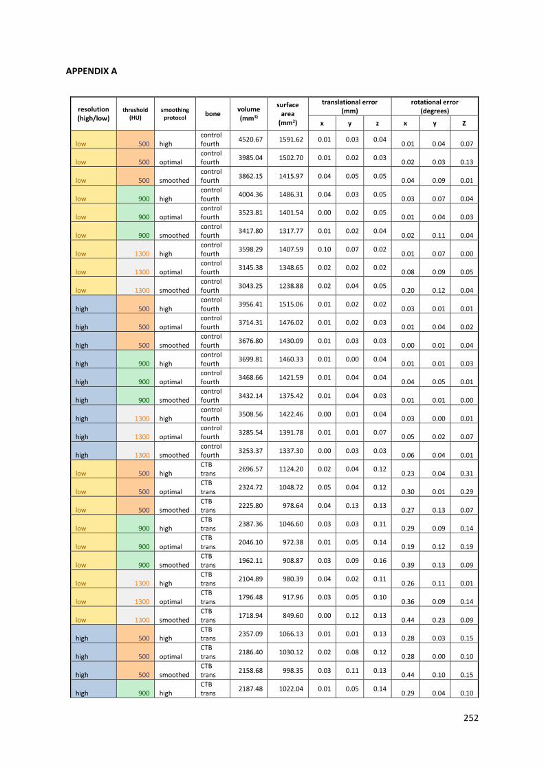
252

APPENDIX A

resolution (high/low)

threshold (HU)

smoothing protocol

bone volume (mm3)

surface area

(mm2)

translational error (mm)

rotational error (degrees)

x y z x y Z

low 500 high control fourth

4520.67 1591.62 0.01 0.03 0.04 0.01 0.04 0.07

low 500 optimal control fourth

3985.04 1502.70 0.01 0.02 0.03 0.02 0.03 0.13

low 500 smoothed control fourth

3862.15 1415.97 0.04 0.05 0.05 0.04 0.09 0.01

low 900 high control fourth

4004.36 1486.31 0.04 0.03 0.05 0.03 0.07 0.04

low 900 optimal control fourth

3523.81 1401.54 0.00 0.02 0.05 0.01 0.04 0.03

low 900 smoothed control fourth

3417.80 1317.77 0.01 0.02 0.04 0.02 0.11 0.04

low 1300 high control fourth

3598.29 1407.59 0.10 0.07 0.02 0.01 0.07 0.00

low 1300 optimal control fourth

3145.38 1348.65 0.02 0.02 0.02 0.08 0.09 0.05

low 1300 smoothed control fourth

3043.25 1238.88 0.02 0.04 0.05 0.20 0.12 0.04

high 500 high control fourth

3956.41 1515.06 0.01 0.02 0.02 0.03 0.01 0.01

high 500 optimal control fourth

3714.31 1476.02 0.01 0.02 0.03 0.01 0.04 0.02

high 500 smoothed control fourth

3676.80 1430.09 0.01 0.03 0.03 0.00 0.01 0.04

high 900 high control fourth

3699.81 1460.33 0.01 0.00 0.04 0.01 0.01 0.03

high 900 optimal control fourth

3468.66 1421.59 0.01 0.04 0.04 0.04 0.05 0.01

high 900 smoothed control fourth

3432.14 1375.42 0.01 0.04 0.03 0.01 0.01 0.00

high 1300 high control fourth

3508.56 1422.46 0.00 0.01 0.04 0.03 0.00 0.01

high 1300 optimal control fourth

3285.54 1391.78 0.01 0.01 0.07 0.05 0.02 0.07

high 1300 smoothed control fourth

3253.37 1337.30 0.00 0.03 0.03 0.06 0.04 0.01

low 500 high CTB trans

2696.57 1124.20 0.02 0.04 0.12 0.23 0.04 0.31

low 500 optimal CTB trans

2324.72 1048.72 0.05 0.04 0.12 0.30 0.01 0.29

low 500 smoothed CTB trans

2225.80 978.64 0.04 0.13 0.13 0.27 0.13 0.07

low 900 high CTB trans

2387.36 1046.60 0.03 0.03 0.11 0.29 0.09 0.14

low 900 optimal CTB trans

2046.10 972.38 0.01 0.05 0.14 0.19 0.12 0.19

low 900 smoothed CTB trans

1962.11 908.87 0.03 0.09 0.16 0.39 0.13 0.09

low 1300 high CTB trans

2104.89 980.39 0.04 0.02 0.11 0.26 0.11 0.01

low 1300 optimal CTB trans

1796.48 917.96 0.03 0.05 0.10 0.36 0.09 0.14

low 1300 smoothed CTB trans

1718.94 849.60 0.00 0.12 0.13 0.44 0.23 0.09

high 500 high CTB trans

2357.09 1066.13 0.01 0.01 0.13 0.28 0.03 0.15

high 500 optimal CTB trans

2186.40 1030.12 0.02 0.08 0.12 0.28 0.00 0.10

high 500 smoothed CTB trans

2158.68 998.35 0.03 0.11 0.13 0.44 0.10 0.15

high 900 high CTB trans

2187.48 1022.04 0.01 0.05 0.14 0.29 0.04 0.10

253

high 900 optimal CTB trans

2025.22 986.84 0.03 0.12 0.12 0.31 0.05 0.05

high 900 smoothed CTB trans

2002.26 956.32 0.02 0.11 0.12 0.28 0.05 0.00

high 1300 high CTB trans

2040.22 985.25 0.03 0.08 0.14 0.39 0.02 0.10

high 1300 optimal CTB trans

1885.47 951.96 0.03 0.07 0.16 0.29 0.04 0.09

high 1300 smoothed CTB trans

1862.88 918.93 0.27 0.10 0.13 0.28 0.03 0.10

low 500 high CTB triple

2758.12 1133.92 0.16 0.01 0.04 0.15 0.12 0.22

low 500 optimal CTB triple

2384.90 1056.25 0.19 0.01 0.07 0.06 0.02 0.17

low 500 smoothed CTB triple

2284.28 987.55 0.22 0.04 0.03 0.06 0.02 0.17

low 900 high CTB triple

2442.13 1056.49 0.19 0.02 0.03 0.45 0.14 0.19

low 900 optimal CTB triple

2091.72 979.62 0.16 0.01 0.07 0.16 0.11 0.17

low 900 smoothed CTB triple

2007.79 917.30 0.19 0.02 0.07 0.10 0.33 0.30

low 1300 high CTB triple

2167.18 992.03 0.16 0.00 0.03 0.31 0.13 0.16

low 1300 optimal CTB triple

1842.74 925.26 0.15 0.03 0.05 0.11 0.09 0.09

low 1300 smoothed CTB triple

1758.97 859.35 0.16 0.01 0.09 0.21 0.34 0.10

high 500 high CTB triple

2394.03 1070.30 0.20 0.02 0.09 0.11 0.07 0.28

high 500 optimal CTB triple

2223.17 1034.21 0.20 0.02 0.06 0.15 0.35 0.43

high 500 smoothed CTB triple

2195.01 1002.96 0.21 0.03 0.06 0.12 0.31 0.15

high 900 high CTB triple

2226.00 1028.77 0.20 0.03 0.10 0.09 0.18 0.30

high 900 optimal CTB triple

2063.20 993.55 0.22 0.04 0.08 0.08 0.18 0.38

high 900 smoothed CTB triple

2039.35 962.40 0.21 0.04 0.06 0.15 0.05 0.35

high 1300 high CTB triple

2090.60 995.10 0.21 0.03 0.07 0.17 0.14 0.35

high 1300 optimal CTB triple

1932.98 962.52 0.21 0.03 0.10 0.11 0.04 0.40

high 1300 smoothed CTB triple

1913.39 929.96 0.21 0.03 0.07 0.18 0.17 0.37

low 500 high First rot 688.64 463.30 0.13 0.37 0.04

low 500 optimal First rot 535.28 409.75 0.23 0.98 0.10

low 500 smoothed First rot 490.03 373.57 0.94 0.98 0.48

low 900 high First rot 513.98 396.69 0.70 0.59 0.93

low 900 optimal First rot 386.77 350.48 0.45 0.58 0.13

low 900 smoothed First rot 345.25 311.02 1.23 1.16 0.67

low 1300 high first rot 356.16 367.64 0.02 0.29 0.59

low 1300 optimal first rot 241.00 341.68 1.20 -0.14 1.27

low 1300 smoothed first rot 210.22 283.46 1.07 -0.06 0.75

high 500 high First rot 539.29 423.69 0.80 -0.08 0.30

high 500 optimal first rot 470.17 397.03 0.69 -0.01 0.99

high 500 smoothed first rot 454.90 378.47 0.61 -0.10 1.10

high 900 high first rot 465.69 389.33 0.74 -0.31 0.65

high 900 optimal first rot 402.65 363.92 0.83 -0.04 0.90

high 900 smoothed first rot 389.47 346.45 0.90 -0.05 1.04

254

high 1300 high first rot 413.42 369.50 1.02 -0.29 1.32

high 1300 optimal first rot 353.76 349.55 0.64 -0.35 1.19

high 1300 smoothed first rot 341.09 325.61 0.65 -0.16 0.72

low 500 high First triple

640.11 447.31 0.00 0.12 0.18 0.28 0.11 0.36

low 500 optimal First triple

497.44 398.07 0.03 0.15 0.14 0.34 0.06 0.04

low 500 smoothed First triple

443.10 356.58 0.06 0.03 0.24 0.07 0.33 0.23

low 900 high First triple

503.60 389.23 0.09 0.14 0.21 0.46 0.63 0.32

low 900 optimal First triple

382.93 347.72 0.08 0.12 0.14 0.52 0.12 0.32

low 900 smoothed First triple

339.25 309.75 0.08 0.07 0.19 0.52 0.13 0.02

low 1300 high First triple

409.87 355.78 0.07 0.20 0.11 2.21 0.46 0.20

low 1300 optimal First triple

305.12 331.73 0.13 0.23 0.09 1.64 0.19 0.23

low 1300 smoothed First triple

264.40 280.03 0.07 0.09 0.11 0.84 0.83 0.11

high 500 high First triple

540.68 421.21 0.05 0.11 0.20 0.39 0.00 0.07

high 500 optimal First triple

470.98 396.13 0.04 0.07 0.23 0.32 0.01 0.09

high 500 smoothed First triple

455.45 379.36 0.01 0.06 0.27 0.18 0.06 0.14

high 900 high First triple

465.07 386.55 0.03 0.10 0.18 0.08 0.02 0.03

high 900 optimal First triple

402.05 363.01 0.06 0.05 0.22 0.27 0.26 0.08

high 900 smoothed First triple

388.05 345.55 0.01 0.05 0.23 0.16 0.26 0.05

high 1300 high First triple

410.41 364.28 0.05 0.06 0.21 0.87 0.07 0.28

high 1300 optimal First triple

352.78 346.69 0.05 0.06 0.18 0.79 0.15 0.26

high 1300 smoothed First triple

338.93 322.86 0.05 0.06 0.22 0.42 0.20 0.18

low 500 high Fourth triple

4426.13 1583.16 0.04 0.22 0.02 0.03 0.06 0.32

low 500 optimal Fourth triple

3890.87 1495.07 0.05 0.24 0.02 0.08 0.11 0.33

low 500 smoothed Fourth triple

3773.69 1404.44 0.05 0.14 0.01 0.11 0.14 0.22

low 900 high Fourth triple

3915.92 1481.10 0.00 0.20 0.01 0.01 0.09 0.55

low 900 optimal Fourth triple

3424.19 1394.84 0.04 0.20 0.03 0.02 0.06 0.33

low 900 smoothed Fourth triple

3322.32 1310.58 0.01 0.19 0.01 0.21 0.11 0.39

low 1300 high Fourth triple

2818.08 1850.05 0.08 0.19 0.03 0.03 0.28 0.39

low 1300 optimal Fourth triple

2198.21 1866.20 0.06 0.25 0.03 0.27 0.27 0.50

low 1300 smoothed Fourth triple

2150.76 1702.81 0.03 0.17 0.01 0.16 0.09 0.23

high 500 high Fourth triple

3881.06 1516.98 0.04 0.22 0.01 0.12 0.12 0.35

high 500 optimal Fourth triple

3635.07 1474.75 0.00 0.18 0.00 0.10 0.18 0.20

high 500 smoothed Fourth triple

3598.36 1431.67 0.00 0.16 0.00 0.10 0.16 0.23

high 900 high Fourth triple

3622.47 1455.14 0.02 0.19 0.03 0.07 0.14 0.25

high 900 optimal Fourth triple

3391.15 1411.84 0.01 0.14 0.00 0.09 0.19 0.25

255

high 900 smoothed Fourth triple

3357.86 1370.10 0.00 0.14 0.00 0.31 0.02 0.30

high 1300 high Fourth triple

3041.48 1932.17 0.02 0.16 0.00 0.21 0.05 0.28

high 1300 optimal Fourth triple

2692.73 2067.13 0.01 0.17 0.03 0.21 0.04 0.24

high 1300 smoothed Fourth triple

2686.96 1880.15 0.01 0.16 0.00 0.27 0.08 0.25

low 500 high second rot 480.74 338.40 2.44 1.23 2.22

low 500 optimal second rot 384.31 299.34 0.51 1.08 0.65

low 500 smoothed second rot 342.08 263.44 0.17 1.36 0.48

low 900 high second rot 380.94 293.56 1.06 0.53 0.03

low 900 optimal second rot 299.78 256.32 0.04 0.74 0.94

low 900 smoothed second rot 262.96 225.99 0.78 0.62 0.39

low 1300 high second rot 311.14 263.06 0.68 0.35 0.19

low 1300 optimal second rot 233.54 237.86 0.37 0.66 1.52

low 1300 smoothed second rot 201.48 201.82 0.00 0.13 0.54

high 500 high second rot 380.71 310.72 0.70 1.35 1.05

high 500 optimal second rot 335.68 291.66 0.00 1.17 0.83

high 500 smoothed second rot 324.00 274.23 0.29 1.05 0.66

high 900 high second rot 338.00 282.72 0.05 1.48 1.00

high 900 optimal second rot 298.20 263.62 0.48 0.79 1.20

high 900 smoothed second rot 286.12 250.00 0.45 0.49 1.30

high 1300 high second rot 295.41 260.80 0.18 0.61 0.90

high 1300 optimal second rot 258.86 242.67 0.42 1.20 1.14

high 1300 smoothed second rot 248.36 228.49 0.15 1.07 1.11

low 500 high Talus trans

7874.30 2632.91 0.09 0.05 0.01 0.03 0.01 0.14

low 500 optimal Talus trans

6921.16 2500.93 0.10 0.04 0.02 0.07 0.05 0.16

low 500 smoothed Talus trans

6741.68 2376.42 0.09 0.06 0.07 0.11 0.02 0.19

low 900 high Talus trans

7075.39 2500.12 0.10 0.06 0.08 0.06 0.05 0.10

low 900 optimal Talus trans

6185.49 2379.31 0.09 0.04 0.02 0.08 0.07 0.06

low 900 smoothed Talus trans

6007.96 2251.82 0.09 0.02 0.03 0.08 0.03 0.14

low 1300 high Talus trans

6400.74 2402.55 0.08 0.05 0.04 0.16 0.16 0.01

low 1300 optimal Talus trans

5558.79 2300.80 0.07 0.01 0.02 0.02 0.11 0.06

low 1300 smoothed Talus trans

5387.67 2148.58 0.07 0.06 0.01 0.09 0.07 0.18

high 500 high Talus trans

6913.69 2553.55 0.09 0.01 0.00 0.03 0.02 0.11

high 500 optimal Talus trans

6479.69 2493.40 0.08 0.04 0.03 0.03 0.01 0.16

high 500 smoothed Talus trans

6422.24 2432.18 0.08 0.04 0.04 0.04 0.04 0.14

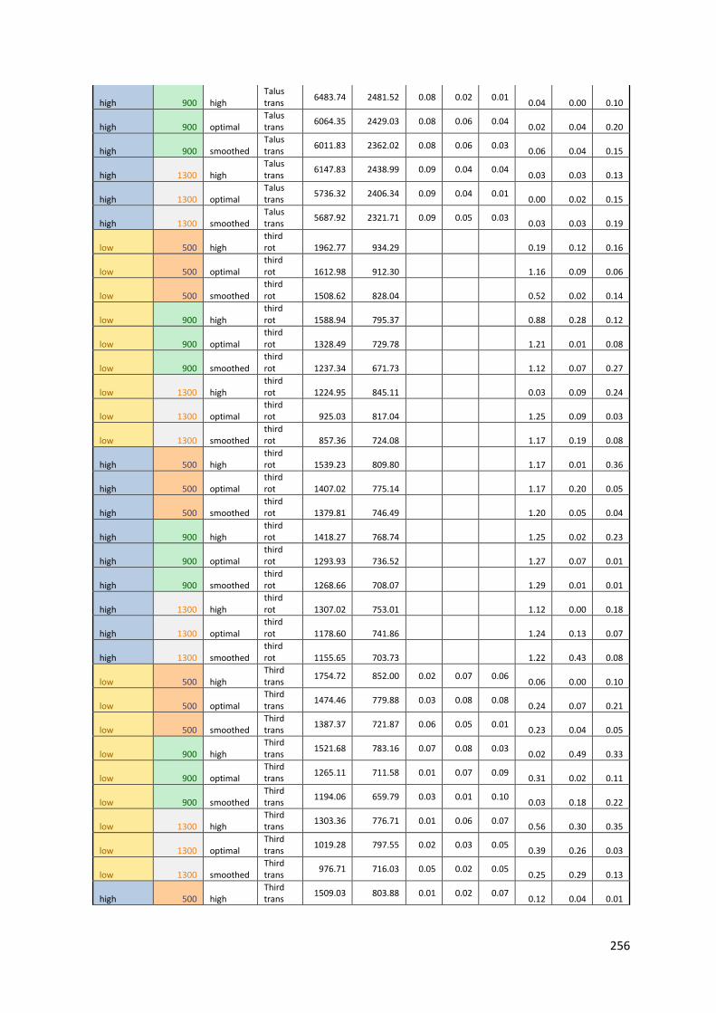
256

high 900 high Talus trans

6483.74 2481.52 0.08 0.02 0.01 0.04 0.00 0.10

high 900 optimal Talus trans

6064.35 2429.03 0.08 0.06 0.04 0.02 0.04 0.20

high 900 smoothed Talus trans

6011.83 2362.02 0.08 0.06 0.03 0.06 0.04 0.15

high 1300 high Talus trans

6147.83 2438.99 0.09 0.04 0.04 0.03 0.03 0.13

high 1300 optimal Talus trans

5736.32 2406.34 0.09 0.04 0.01 0.00 0.02 0.15

high 1300 smoothed Talus trans

5687.92 2321.71 0.09 0.05 0.03 0.03 0.03 0.19

low 500 high third rot 1962.77 934.29 0.19 0.12 0.16

low 500 optimal third rot 1612.98 912.30 1.16 0.09 0.06

low 500 smoothed third rot 1508.62 828.04 0.52 0.02 0.14

low 900 high third rot 1588.94 795.37 0.88 0.28 0.12

low 900 optimal third rot 1328.49 729.78 1.21 0.01 0.08

low 900 smoothed third rot 1237.34 671.73 1.12 0.07 0.27

low 1300 high third rot 1224.95 845.11 0.03 0.09 0.24

low 1300 optimal third rot 925.03 817.04 1.25 0.09 0.03

low 1300 smoothed third rot 857.36 724.08 1.17 0.19 0.08

high 500 high third rot 1539.23 809.80 1.17 0.01 0.36

high 500 optimal third rot 1407.02 775.14 1.17 0.20 0.05

high 500 smoothed third rot 1379.81 746.49 1.20 0.05 0.04

high 900 high third rot 1418.27 768.74 1.25 0.02 0.23

high 900 optimal third rot 1293.93 736.52 1.27 0.07 0.01

high 900 smoothed third rot 1268.66 708.07 1.29 0.01 0.01

high 1300 high third rot 1307.02 753.01 1.12 0.00 0.18

high 1300 optimal third rot 1178.60 741.86 1.24 0.13 0.07

high 1300 smoothed third rot 1155.65 703.73 1.22 0.43 0.08

low 500 high Third trans

1754.72 852.00 0.02 0.07 0.06 0.06 0.00 0.10

low 500 optimal Third trans

1474.46 779.88 0.03 0.08 0.08 0.24 0.07 0.21

low 500 smoothed Third trans

1387.37 721.87 0.06 0.05 0.01 0.23 0.04 0.05

low 900 high Third trans

1521.68 783.16 0.07 0.08 0.03 0.02 0.49 0.33

low 900 optimal Third trans

1265.11 711.58 0.01 0.07 0.09 0.31 0.02 0.11

low 900 smoothed Third trans

1194.06 659.79 0.03 0.01 0.10 0.03 0.18 0.22

low 1300 high Third trans

1303.36 776.71 0.01 0.06 0.07 0.56 0.30 0.35

low 1300 optimal Third trans

1019.28 797.55 0.02 0.03 0.05 0.39 0.26 0.03

low 1300 smoothed Third trans

976.71 716.03 0.05 0.02 0.05 0.25 0.29 0.13

high 500 high Third trans

1509.03 803.88 0.01 0.02 0.07 0.12 0.04 0.01

257

high 500 optimal Third trans

1374.87 767.66 0.02 0.01 0.06 0.17 0.17 0.01

high 500 smoothed Third trans

1352.30 739.55 0.02 0.03 0.01 0.08 0.22 0.24

high 900 high Third trans

1377.09 762.41 0.00 0.02 0.06 0.01 0.07 0.13

high 900 optimal Third trans

1252.45 727.24 0.02 0.01 0.05 0.18 0.20 0.03

high 900 smoothed Third trans

1230.41 701.72 0.01 0.01 0.04 0.05 0.04 0.06

high 1300 high Third trans

1216.09 835.14 0.02 0.01 0.07 0.19 0.02 0.10

high 1300 optimal Third trans

1068.23 850.58 0.02 0.01 0.09 0.19 0.05 0.06

high 1300 smoothed Third trans

1053.48 796.34 0.02 0.01 0.05 0.25 0.06 0.08

258

APPENDIX B:

A Givens rotation is a rotation in the plane acting on two elements of a given vector. It can be represented in matrix form as

where the \cos{\theta} and \sin{\theta} appear at the intersection of the ith and jth rows and columns. When acting on a vector x, G(i,j,\theta) x performs a rotation of the (i,j) elements of x. Givens rotations are typically used to introduce zeros in vectors, such as during the QR decomposition of a matrix. In this case, it is typically desired to find c and s such that

with r = \sqrt{a^2 + b^2}.

Function: void gsl_linalg_givens (const double a, const double b, double * c, double * s)

This function computes c = \cos{\theta} and s = \sin{\theta} so that the Givens matrix G(\theta) acting on the vector (a,b) produces (r, 0), with r = \sqrt{a^2 + b^2}.

Function: void gsl_linalg_givens_gv (gsl_vector * v, const size_t i, const size_t j, const double c, const double s)

This function applies the Givens rotation defined by c = \cos{\theta} and s = \sin{\theta} to the i and j elements of v. On output, (v(i),v(j)) \leftarrow G(\theta) (v(i),v(j)).

(*ref: GNU Scientific Library – reference Manual: Givens Rotations: https://www.gnu.org/software/gsl/manual/html_node/Givens-Rotations.html*)

259

APPENDIX C:

vectors for helical axis of individual bones loaded to force

specimens name point x point y point z vector X vector Y vector Z

1L calcaneus -41.52 2.72 -5.79 -0.79 0.60 -0.12

1R calcaneus -40.29 6.11 -5.91 -0.79 0.61 -0.06

2L calcaneus -52.06 0.34 -1.20 -0.62 0.62 -0.47

2R calcaneus -76.55 -8.48 20.69 -0.66 0.54 -0.52

3L calcaneus -46.82 3.94 -1.32 -0.60 0.78 -0.19

3R calcaneus -49.53 3.30 0.08 -0.70 0.67 -0.23

4L calcaneus -42.95 2.11 -3.31 -0.77 0.59 -0.24

4R calcaneus -43.83 3.61 -4.31 -0.79 0.55 -0.27

5L calcaneus -50.11 1.62 1.78 -0.79 0.56 -0.24

5R calcaneus -54.30 -24.54 25.58 -0.99 0.12 -0.13

1L CTB -23.20 -10.60 -4.09 -0.50 0.83 -0.24

1R CTB -20.65 -7.63 -6.86 -0.48 0.87 -0.07

2L CTB -31.46 -10.41 -1.07 -0.29 0.87 -0.39

2R CTB -36.24 -12.68 9.55 -0.55 0.69 -0.46

3L CTB -28.23 -14.77 -0.28 -0.54 0.84 -0.07

3R CTB -30.29 -13.55 2.98 -0.58 0.81 -0.10

4L CTB -24.51 -13.19 1.61 -0.40 0.89 -0.21

4R CTB -26.50 -10.80 1.04 -0.37 0.91 -0.19

5L CTB -21.44 -11.90 2.45 -0.73 0.68 -0.04

5R CTB -25.67 -16.10 4.88 -0.85 0.50 -0.16

1L fourth -26.10 -4.15 -5.72 -0.55 0.79 -0.26

1R fourth -22.20 -1.25 -7.47 -0.58 0.79 -0.19

2L fourth -30.66 -3.36 -2.27 -0.45 0.77 -0.44

2R fourth -33.32 -0.08 1.19 -0.47 0.71 -0.53

3L fourth -31.94 -5.14 -2.13 -0.41 0.88 -0.23

3R fourth -31.82 -4.98 -0.61 -0.55 0.80 -0.24

4L fourth -25.87 -2.92 -1.76 -0.36 0.90 -0.26

4R fourth -26.42 0.43 -3.78 -0.30 0.92 -0.24

5L fourth -23.64 -5.95 1.12 -0.71 0.66 -0.26

5R fourth -27.49 -3.39 -0.77 -0.62 0.65 -0.43

1L MTIII -7.84 1.80 -14.18 0.11 0.97 -0.22

1R MTIII -5.70 0.17 -11.34 0.02 1.00 -0.08

2L MTIII -7.79 9.18 -13.35 0.28 0.92 -0.29

2R MTIII -4.57 11.75 -12.12 0.26 0.95 -0.19

3L MTIII -13.95 -2.89 -6.68 0.06 0.99 -0.08

3R MTIII -15.31 -5.48 -5.92 -0.05 0.98 -0.17

4L MTIII -9.67 1.98 -6.23 0.10 0.97 -0.23

4R MTIII -11.11 0.65 -5.98 0.04 0.99 -0.14

5L MTIII -9.66 -7.66 -0.94 -0.12 0.97 -0.21

5R MTIII -4.43 8.12 -9.85 0.28 0.94 -0.20

1L MTII -9.32 -3.99 -13.82 0.12 0.97 -0.22

260

1R MTII -8.62 -5.14 -11.68 0.04 0.99 -0.15

2L MTII -12.67 -3.21 -10.16 0.14 0.92 -0.35

2R MTII -9.10 0.67 -9.61 0.16 0.93 -0.32

3L MTII -16.28 -8.95 -6.32 0.06 0.99 -0.15

3R MTII -17.85 -11.02 -4.99 -0.05 0.97 -0.23

4L MTII -12.99 -3.23 -6.50 0.12 0.94 -0.31

4R MTII -12.07 -6.16 -4.84 0.02 0.98 -0.20

5L MTII -13.05 -12.11 -0.66 -0.09 0.96 -0.28

5R MTII -8.93 -0.68 -9.03 0.22 0.94 -0.24

1L MTIV -7.42 -2.17 -12.05 -0.16 0.92 -0.36

1R MTIV -4.02 -2.32 -11.00 -0.22 0.95 -0.20

2L MTIV -9.65 2.50 -9.66 -0.04 0.93 -0.37

2R MTIV -5.10 1.59 -6.63 -0.16 0.95 -0.27

3L MTIV -10.55 -12.02 -4.46 -0.29 0.94 -0.15

3R MTIV -7.92 -11.73 -3.96 -0.38 0.89 -0.25

4L MTIV -8.87 1.11 -5.45 -0.08 0.96 -0.28

4R MTIV -9.89 4.06 -6.56 -0.06 0.99 -0.16

5L MTIV 4.80 -15.35 2.01 -0.53 0.81 -0.24

5R MTIV -1.25 -5.95 -3.03 -0.30 0.89 -0.34

1L MTV -10.37 5.35 -15.73 -0.13 0.93 -0.36

1R MTV -5.75 3.55 -13.42 -0.22 0.96 -0.16

2L MTV -9.69 11.98 -13.97 0.02 0.94 -0.33

2R MTV -6.55 13.81 -12.66 -0.01 0.97 -0.24

3L MTV -11.84 -7.96 -5.89 -0.33 0.93 -0.15

3R MTV -10.27 -6.61 -5.90 -0.39 0.88 -0.25

4L MTV -11.45 6.06 -7.26 -0.10 0.96 -0.27

4R MTV -12.63 11.32 -8.76 -0.03 0.99 -0.15

5L MTV -0.12 -8.75 -0.72 -0.50 0.83 -0.24

5R MTV -5.16 0.13 -6.39 -0.29 0.91 -0.31

1L second -16.17 -11.49 -7.70 -0.25 0.91 -0.34

1R second -14.83 -7.17 -9.28 -0.13 0.98 -0.16

2L second -19.53 -13.27 -2.95 -0.24 0.89 -0.39

2R second -18.23 -6.21 -4.50 0.01 0.80 -0.60

3L second -23.38 -16.22 -3.54 -0.22 0.98 0.01

3R second -26.36 -21.61 5.81 -0.65 0.74 -0.18

4L second -16.84 -13.37 -1.46 -0.14 0.98 -0.17

4R second -19.08 -9.00 -3.70 -0.02 0.92 -0.40

5L second -20.46 -18.77 5.92 -0.60 0.75 -0.27

5R second -22.07 -14.46 1.52 -0.32 0.92 -0.24

1L third -21.25 -7.81 -7.37 -0.27 0.93 -0.24

1R third -19.10 -5.21 -8.49 -0.30 0.93 -0.21

2L third -26.02 -5.20 -5.95 -0.04 0.92 -0.39

2R third -25.07 -0.03 -7.05 0.04 0.93 -0.37

3L third -26.63 -12.35 -2.55 -0.27 0.95 -0.15

3R third -26.70 -11.10 -0.78 -0.39 0.90 -0.19

261

4L third -22.85 -8.63 -1.77 -0.14 0.95 -0.27

4R third -24.20 -7.07 -2.24 -0.20 0.95 -0.23

5L third -22.18 -15.03 6.08 -0.60 0.78 -0.15

5R third -25.68 -11.19 1.11 -0.38 0.87 -0.32

1L tibia -36.19 -3.74 -4.35 0.05 -0.99 0.16

1R tibia -35.02 -4.67 -4.07 -0.03 -0.99 0.16

2L tibia -41.11 -0.71 -2.73 0.13 -0.99 0.09

2R tibia -37.59 -0.29 -0.21 0.12 -0.99 0.12

3L tibia -41.25 -4.62 -0.16 -0.06 -1.00 0.02

3R tibia -41.86 -2.05 0.34 -0.03 -1.00 0.08

4L tibia -37.89 -4.66 0.38 0.06 -0.99 0.12

4R tibia -38.87 0.12 -1.56 0.08 -1.00 0.05

5L tibia -41.04 2.80 1.45 0.00 -1.00 0.04

5R tibia -44.41 0.23 0.78 0.03 -1.00 0.09

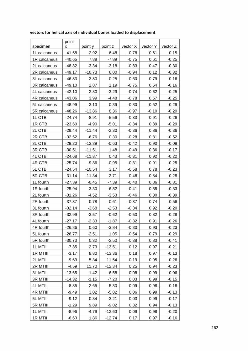
262

vectors for helical axis of individual bones loaded to displacement

specimen point x point y point z vector X vector Y vector Z

1L calcaneus -41.58 2.92 -6.48 -0.78 0.61 -0.15

1R calcaneus -40.65 7.88 -7.89 -0.75 0.61 -0.25

2L calcaneus -48.82 -3.34 -3.18 -0.83 0.47 -0.30

2R calcaneus -49.17 -10.73 6.00 -0.94 0.12 -0.32

3L calcaneus -46.83 3.80 -0.25 -0.60 0.79 -0.16

3R calcaneus -49.10 2.87 1.19 -0.75 0.64 -0.16

4L calcaneus -42.10 2.80 -3.29 -0.74 0.62 -0.25

4R calcaneus -43.06 3.99 -4.48 -0.78 0.57 -0.25

5L calcaneus -48.99 3.13 0.39 -0.80 0.52 -0.29

5R calcaneus -48.26 -13.86 8.36 -0.97 -0.10 -0.20

1L CTB -24.74 -8.91 -5.56 -0.33 0.91 -0.26

1R CTB -23.60 -4.90 -5.01 -0.34 0.89 -0.29

2L CTB -29.44 -11.44 -2.30 -0.36 0.86 -0.36

2R CTB -32.52 -6.76 0.30 -0.28 0.81 -0.52

3L CTB -29.20 -13.39 -0.63 -0.42 0.90 -0.08

3R CTB -30.51 -11.51 1.48 -0.49 0.86 -0.17

4L CTB -24.68 -11.87 0.43 -0.31 0.92 -0.22

4R CTB -25.74 -9.36 -0.95 -0.31 0.91 -0.25

5L CTB -24.54 -10.54 3.17 -0.58 0.78 -0.23

5R CTB -31.14 -11.34 2.71 -0.46 0.84 -0.28

1L fourth -27.39 -0.45 -7.39 -0.40 0.86 -0.31

1R fourth -25.94 3.30 -6.82 -0.41 0.85 -0.33

2L fourth -31.26 -4.52 -3.53 -0.46 0.80 -0.39

2R fourth -37.87 0.78 -0.61 -0.37 0.74 -0.56

3L fourth -32.14 -3.68 -2.53 -0.34 0.92 -0.20

3R fourth -32.99 -3.57 -0.62 -0.50 0.82 -0.28

4L fourth -27.17 -2.33 -1.87 -0.32 0.91 -0.26

4R fourth -26.86 0.60 -3.84 -0.30 0.93 -0.23

5L fourth -26.77 -2.51 1.05 -0.54 0.79 -0.29

5R fourth -30.73 0.32 -2.50 -0.38 0.83 -0.41

1L MTIII -7.35 2.73 -13.51 0.12 0.97 -0.21

1R MTIII -3.17 8.80 -13.36 0.18 0.97 -0.13

2L MTIII -9.69 5.34 -11.54 0.19 0.95 -0.26

2R MTIII -4.59 11.70 -12.34 0.25 0.94 -0.23

3L MTIII -13.65 -1.42 -6.58 0.08 0.99 -0.06

3R MTIII -14.32 -1.15 -7.20 0.03 0.99 -0.15

4L MTIII -8.85 2.65 -5.30 0.09 0.98 -0.18

4R MTIII -9.49 3.02 -5.82 0.06 0.99 -0.13

5L MTIII -9.12 0.34 -3.21 0.03 0.99 -0.17

5R MTIII -1.29 9.89 -9.02 0.32 0.94 -0.13

1L MTII -8.96 -4.79 -12.63 0.09 0.98 -0.20

1R MTII -6.63 1.86 -12.74 0.17 0.97 -0.16

263

2L MTII -12.20 -2.37 -10.24 0.15 0.95 -0.28

2R MTII -5.57 8.13 -13.22 0.32 0.91 -0.27

3L MTII -15.87 -8.19 -6.36 0.08 0.99 -0.10

3R MTII -16.49 -10.46 -5.61 -0.04 0.98 -0.20

4L MTII -10.68 -3.02 -5.19 0.12 0.98 -0.18

4R MTII -9.69 -0.46 -6.41 0.12 0.99 -0.10

5L MTII -11.26 -1.98 -4.23 0.13 0.98 -0.16

5R MTII -2.78 6.06 -9.68 0.40 0.91 -0.08

1L MTIV -6.62 -1.33 -11.80 -0.15 0.93 -0.35

1R MTIV -4.37 3.66 -11.80 -0.10 0.95 -0.29

2L MTIV -9.67 -1.65 -8.07 -0.13 0.92 -0.37

2R MTIV -5.87 4.28 -8.52 -0.10 0.94 -0.33

3L MTIV -12.19 -9.03 -4.61 -0.23 0.96 -0.15

3R MTIV -8.62 -9.76 -4.28 -0.34 0.90 -0.27

4L MTIV -8.93 -1.28 -3.67 -0.13 0.95 -0.27

4R MTIV -9.88 3.55 -5.91 -0.08 0.98 -0.19

5L MTIV -0.52 -10.35 0.68 -0.40 0.88 -0.26

5R MTIV -3.90 -1.07 -5.07 -0.17 0.94 -0.31

1L MTV -9.31 4.52 -14.56 -0.15 0.93 -0.35

1R MTV -6.70 9.25 -14.07 -0.11 0.95 -0.28

2L MTV -11.38 6.57 -11.64 -0.10 0.93 -0.35

2R MTV -7.69 15.79 -14.22 0.03 0.95 -0.31

3L MTV -14.59 -2.90 -6.48 -0.23 0.96 -0.16

3R MTV -12.63 -3.15 -6.88 -0.32 0.91 -0.27

4L MTV -11.44 3.37 -5.30 -0.16 0.95 -0.28

4R MTV -12.66 9.78 -7.93 -0.07 0.98 -0.20

5L MTV -2.95 -4.57 -1.59 -0.41 0.87 -0.27

5R MTV -4.98 1.89 -6.66 -0.25 0.92 -0.31

1L second -22.46 -11.24 -6.36 -0.20 0.90 -0.38

1R second -14.95 -7.27 -7.59 -0.17 0.98 -0.09

2L second -21.63 -12.02 -4.71 -0.11 0.96 -0.25

2R second -11.09 -13.20 4.19 -0.63 0.77 0.04

3L second -20.15 -18.44 -2.37 -0.26 0.85 0.45

3R second -49.62 -14.79 5.67 -0.27 0.78 -0.56

4L second -22.66 -13.43 -1.00 -0.14 0.95 -0.29

4R second -23.23 -11.71 -1.84 -0.17 0.93 -0.33

5L second -21.18 -15.99 4.81 -0.40 0.92 -0.02

5R second -29.42 -11.09 -0.51 -0.07 0.92 -0.38

1L third -22.49 -5.65 -8.69 -0.16 0.94 -0.30

1R third -20.53 -1.57 -8.66 -0.14 0.94 -0.30

2L third -26.82 -7.53 -5.74 -0.15 0.90 -0.40

2R third -28.28 -0.62 -6.82 0.00 0.86 -0.51

3L third -27.23 -11.65 -2.03 -0.23 0.96 -0.13

3R third -28.72 -9.62 -1.27 -0.31 0.93 -0.22

4L third -23.10 -9.23 -1.44 -0.18 0.94 -0.29

264

4R third -24.49 -6.52 -2.93 -0.18 0.95 -0.25

5L third -25.31 -9.50 2.80 -0.34 0.91 -0.24

5R third -27.73 -6.51 -2.78 -0.09 0.95 -0.29

1L tibia -36.05 -3.42 -4.21 0.05 -0.99 0.15

1R tibia -34.77 -2.55 -4.70 0.00 -0.99 0.14

2L tibia -40.61 -1.88 -2.16 0.11 -0.99 0.09

2R tibia -37.73 -1.34 -0.17 0.12 -0.98 0.13

3L tibia -41.22 -4.34 -0.18 -0.06 -1.00 0.01

3R tibia -41.74 -0.69 0.45 -0.02 -1.00 0.07

4L tibia -38.09 -5.06 0.28 0.06 -0.99 0.12

4R tibia -38.74 -1.10 -1.17 0.09 -0.99 0.07

5L tibia -41.37 3.90 1.29 0.01 -1.00 0.04

5R tibia -44.77 0.44 0.55 0.03 -1.00 0.08

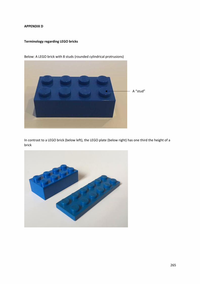
265

APPENDIX D

Terminology regarding LEGO bricks

Below: A LEGO brick with 8 studs (rounded cylindrical protrusions)

In contrast to a LEGO brick (below left), the LEGO plate (below right) has one third the height of a

brick

A “stud”

266

Motion of LEGO bricks.

A blue 8 stud LEGO brick has been placed on a green LEGO board below.

This brick can now be moved in three directions along the 3 cardinal axes.

Moved “sideways” by one stud

Moved “backwards” by one stud

Moved “up” by the thickness of one plate