the effect of interpolation methods on the …

A. Šiljeg i dr. Utjecaj metoda interpolacije na kvalitetu digitalnih modela reljefa za geomorfometrijske analize

Tehnički vjesnik 22, 5(2015), 1149-1156 1149

ISSN 1330-3651 (Print), ISSN 1848-6339 (Online) DOI: 10.17559/TV-20131010223216

THE EFFECT OF INTERPOLATION METHODS ON THE QUALITY OF A DIGITAL TERRAIN MODEL FOR GEOMORPHOMETRIC ANALYSES

Ante Šiljeg, Sanja Lozić, Denis Radoš

Original scientific paper Despite the modern technological advancements, contemporary methods of data gathering still rely on point samples, which means they feature a precise variable info only on specific x, y - coordinates. In order to get a continual representation of a surface necessary for research, it is necessary to approximate various data values on those surfaces which have not been sampled by using various methods of interpolation. The main aim of this research is to evaluate two different methods of interpolation based on the quality of digital terrain models used for geomorphometric analyses. For the purposes of developing and comparing these methods, a set of elevation data was attained by vectorization of contour lines from HOK. Two methods of interpolation were tested: triangulated irregular network (TIN) and ANUDEM (Topo to Raster). In order to get a more appropriate method, the research employed eight statistical parameters, various graphical representations (both two- and three-dimensional) and geomorphometric parameter of slope inclination. The research shows that ANUDEM is a better method for geomorphometric analyses than TIN is. After the analysis of geomorphometric parameters (slope), the conclusion is that there are no significant differences between the digital terrain models developed on the bases of different sets of elevation data. Keywords: digital terrain model; HOK; interpolation methods; root mean square error; vectorization Utjecaj metoda interpolacije na kvalitetu digitalnih modela reljefa za geomorfometrijske analize

Izvorni znanstveni članak Danas su, bez obzira na rapidni razvoj tehnologije, većina prikupljenih (izmjerenih) podataka točkasti uzorci, dakle imaju točnu vrijednost odabrane varijable samo na izmjerenim x, y koordinatama. Da bi se dobile kontinuirane površine koje su neophodne za proučavanje, potrebno je procijeniti vrijednosti na neuzorkovanim područjima koristeći pritom različite metode interpolacije. Glavni cilj ovog istraživanja je vrednovanje dviju metoda interpolacije na kvalitetu digitalnih modela reljefa za potrebe geomorfometrijskih istraživanja. Za izradu modela i usporedbu metoda interpolacije korišten je skup visinskih podatka dobiven vektorizacijom izohipsi s HOK-a. Testirane su dvije metode interpolacije: triangulacijska nepravilna mreža (TIN) i ANUDEM (Topo to Raster). Za odabir prikladnije metode interpolacije korišteno je 8 statističkih parametara, grafički prikazi (dvodimenzionalni i trodimenzionalni), i geomorfometrijski parametar (nagib padina). Utvrđeno je da je ANUDEM bolja metoda za geomorfometrijska istraživanja od TIN-a. Analizom geomorfometrijskog parametra (nagib) zaključeno je da ne postoje značajnije razlike između DMR dobivenih iz različitih skupova visinskih podataka. Ključne riječi: digitalni model reljefa; HOK; metode interpolacije; srednja kvadratna pogreška; vektorizacija 1 Introduction

Since the middle of 20th century, various techniques of digital representation and analysis of terrain have developed, due to the rapid development of computer technology, mathematics and computer graphics [31, 32]. In the concept of terrain representation, one of the most important notions is the digital terrain model [24]. The process of quantitative digital terrain analysis is known as digital geomorphometry [32], digital terrain analysis or DTA [47,16] and digital terrain modeling or DTM [27, 45, 24]. One of the main goals of geomorphometry is to develop and analyze DTM. Simply put, a digital terrain model is a statistical representation of continual terrain surfaces (vector or raster) with a set of known x, y and z coordinates within a custom coordinate system [25].

Scientific literature has not yet established a single term for it, which means that various terms are used depending on the scientific discipline which employs it or a country in which the research was conducted. This research generally uses the term digital terrain model to describe the entire area of Lake Vrana Nature Park attained by vectorization and interpolation of contour lines from HOK. A digital terrain model is a simplified representation of a part of terrain in raster form and features a specific resolution. It was developed by scientifically based method of interpolation of elevation data attained by a specific measurement and analysis method [40]. Despite the modern technological advancements, contemporary methods of data gathering

still rely on point samples, which means they feature a precise variable info only on specific x, y - coordinates. In order to get a continual representation of a surface necessary for research and knowledge about our living space, it is necessary to approximate various data values on those surfaces which have not been sampled by using various methods of interpolation [22, 18, 28]. Each method results in different results, so the main challenge is to generate the most accurate surface on the basis of available data and to determine the characteristics of errors and variation of values by comparing different interpolation methods. There are several interpolation methods [10, 37, 44].

Two methods of interpolation were analyzed and compared in this research: TIN and ANUDEM. The most appropriate method for geomorphometric analysis was chosen on the basis of eight established parameters (variables). The success of interpolation method was determined by these variables. All the parameters are important when determining the most appropriate method, but the most observed parameter was standard deviation or root mean square error, which is the most used parameter world-wide for determining the accuracy of digital models [49, 1]. In addition to statistical parameters, the methods were compared in terms of graphical representations (two- and three-dimensional) and by geomorphometric parameter of slope inclination.

There are five methods of gathering data (elevation points) for digital terrain models: 1) field measuring, 2) photogrammetric data gathering, 3) laser recording

The effect of interpolation methods on the quality of a digital terrain model for geomorphometric analyses A. Šiljeg et al.

1150 Technical Gazette 22, 5(2015), 1149-1156

(scanning), 4) radar data gathering and 5) vectorising the existing topographic maps [40].

The accuracy of interpolation methods was tested by comparing the elevation point-data gathered by photogrammetry and stereo-restitution to the data generated by raster models from HOK’s contour lines. In addition, the research determined the differences between various sets of elevation data by analysing the morphometric parameter of slope inclination.

There are various programs and modules used for interpolation of the measured data in order to create a correct quadratic network, which is used for analysis and visualization [29, 48, 15]. For the processes of interpolation, analysis and interpretation of the gathered data two extensions were used, 3DAnalyst and Hawts tool, both integrated into ArcGISDesktop. 2 Methods and results 2.1 Triangulated irregular network

Triangulated irregular network (TIN) is a method of interpolation employed by linear and non-linear functions for the approximation of unknown values [35, 26]. In TIN method, all point-samples are connected by a series of triangles, mostly based on Delaunay’s triangulation (linear function) [43]. Every triangle is a section of a plane determined by three edges and vertices. For every triangle (ABC) there is a rule stating that every point apart from A, B and C is outside its circumcircle (Fig. 1).

Figure 1 Delaunay triangulation principle

In order to transpose the triangulation problem into a

plane, it is important to note that a terrain cannot have multiple points on the same x and y coordinates and the same elevation [12]. Delaunay plane triangulation starts from the premise that the points in xy-plane are projected onto a paraboloid z=x2+y2 parallel to z-axis, a condition that meets the triangulation rule of the least possible number of sharp angles (optimal solution) [12]. The unknown values of points are determined mostly via one of the fastest and simplest algorithms, the so-called improving algorithm. The basis of this algorithm is the addition of n unknown points into the existing network (Delaunay network 1 – DN1), which follows the rule of removing any triangles with circumcircles containing the new point (Pv) (Fig. 1). In this way a new network of triangles is constructed (Delaunay network 2 – DN2) according to previously set rules, and this action repeats (Fig. 1). TIN is a method which had a wide range of applications, although most of authors point out numerous

deficiencies, mostly in cases when the distance between the points is large [4, 26]. With the development of aero and terrestrial laser data gathering technology (elevation density), TIN is showing up as an optimal method [2]. 2.2 ANUDEM (Australian National University DEM) or Topo

to Raster

ANUDEM is an interpolation method specifically designed for generating hydrologically accurate digital terrain model [7, 6]. This interpolation method was developed at Australian National University, but is widely used in many countries and research papers [23, 50].With its erosive effects, water affects the terrain in a significant manner, so it is important to accurately describe relations in a complicated drainage system within a digital model. The method is based on the ANUDEM program developed by Hutchinson [19] and is in fact a modified version of thin-plate spline method, which takes into consideration significant changes in terrain, such as ridges, ravines, creeks etc. [42]. This method employs Gauss-Seidel iterative calculating method [7, 30], which is optimized to be effective as a local interpolation method (for example, inverse distance) but without the loss of area continuity characteristic of global interpolation methods [7]. Dissection is defined as first and second degree of partial derivation f of the interpolation method described by the following equations [30]:

yxfffJ yx d)d()( 22

1 += ∫ , (1)

yxffffJ yyxyxx d)d2()( 2222 ++= ∫ . (2)

Minimizing J2 results in an unrealistically flat

surface, while minimizing J1 creates a more protrusive local maximum and minimum on samples that feature better resolution. Hutchinson [19] found a better empirical compromise between J1 and J2, by defining the algorithm for dissection according to formula [30]:

)()(50)( 21

2 fJfJh,fJ +×= − , (3) where h stands for spatial resolution.

Hutchinson (1996) implemented a spatially variable statistical estimation for error by introducing a quadratic network to display elevation. This modification results in a level of flattening which adjusts to local terrain slopes. The purpose of the method is to identify and remove any "false" local erosion bases (sinks) in the output model, since the program assumes that all the unknown sinks are in fact errors , considering their presence in the nature is very rare [13]. The algorithm does not remove those sinks that have a vertical difference higher than specified by the user via vertical tolerance (the usual value is half the equidistance). The algorithm enables the input of data pertaining to stream lines, which means every stream can be adjusted to the valley’s bottom. In addition, the algorithm prefers the use of contour lines as primary input data in order to generate a correct model, since it is based



on the identification of the most significant curvature on each contour line. 2.3 Generating DTM from data attained by vectorization of

contour lines

Contour lines obtained from HOK were interpolated by experts for stereo-restitution by using methods and techniques which were available during the creation of maps. Regardless of the fact that the newer data, attained and processed by modern photogrammetry, is geodetically more accurate in terms of location and elevation (the maps were first scanned and then geo-referenced), the analysis of the terrain in Vrana Lake Nature Park can be made by vectorising and interpolation contour lines from HOK. The reasons are the following: 1) lower spatial resolution enables a more realistic display of sudden terrain changes, as opposed to 25-meter resolution suggested by DGU (2003) (for data acquired by aero-photogrammetry) which flattens the surface and usually ignores some important details in the terrain; 2) for the purpose of determining elevation values, various aero-photogrammetry methods were used, which employed a detailed precise levelling (up to a millimetre level of accuracy); 3) contour lines are manually interpolated and 4) the developed model clearly shows a realistic approximation. 2.4 Accuracy of HOK1

Since the WW I, cartographic development was mostly connected with military institutions outside Croatia. All topographic maps (except map 1:5000) were made in the Military Geographical Institute in Belgrade, which still has the original versions, while only a number of copies remained in the Republic of Croatia [17]. During the 1960s, topographic cards with scale 1:5000 started to be developed in Croatia as well, first by aero-photogrammetry and precise levelling, and later exclusively by aero-photogrammetry. The original papers of such maps were made on drawing foils. It is important to note that these maps were made with high scientific and expert standards, and that their quality in terms of technicality is impeccable [3]. A study was made, named "Study about the substitution of the originals and renovation of the content of topographic maps"[3], which aimed at gaining at least a partial insight into the accuracy of 1:5000 maps. The study tested the accuracy of coordinate network as well as geodetic basis, on the case of several papers of the 1:5000 map. Root mean square error of the coordinate network was approximately ±0,7m, while the root mean square error of the geodetic basis was between ±0,58 m and ±1,50 m. The accuracy of the map is directly connected to the accuracy of photogrammetric restitution. The accuracy of aero-triangulation is 4 µm = ±0,12 m. The accuracy of restitution of line and point elements on analytical stereo-instruments in 10 µm = ±0,30 m. The maximum error is approximately ±1 m [3]. 1 HOK (hrvatska osnovna karta) eng. Croatian base map

2.5 Vectorization of contour lines

The values of elevation data necessary for the development of DTM of Vrana Lake Nature Park were obtained by vectorising the contour lines from Croatian basic maps in 1:5000 scale. Contour lines on digital raster maps represent lines which connect the areas of the same elevation with the equidistance of 5 meters. Before the process of vectorization, contour lines in raster model can essentially have an infinite number of elevation data. However, during the vectorization process, a specific number points is defined within each line that represent elevation data, and this number depends on the chosen method. Vectorization is process of transforming raster model of data into vector model, and can be manual, semiautomatic or automatic. Manual vectorization is physically most demanding, since it includes three activities: preparation of the original, navigation of the pointer across previously defined objects and, finally, adding attributes. Automatic vectorization means that the entire process is automatic and based on various algorithms which detect and evaluate raster content [5]. Considering that the automatic vectorization from HOK resources is virtually impossible due to their low resolution and numerous objects on the maps (roads, names, dry-stone walls, water streams etc.), this research employed manual and semi-automatic vectorization. In semiautomatic vectorization, a contour line is automatically vectorised up until the first obstruction, such as crossing another contour line, which means that the operator has to manually take the cursor over the crossing and onto the line which is being vectorised [11].

Figure 2 An example of semiautomatic (a) and manual (b) vectorization

of contour lines.

Semiautomatic vectorization was made by the program WinTopo. Nineteen pages of HOK maps were used. The process of vectorization included several steps2: 1) adding the pages to the program (individually), 2) selecting contour lines in raster model (sampling colours) 2 Vectorization process on smaller scale maps (e.g. 1:25 000) is more complicated due to more contents (intersecting layers) [33, 34].

a

b



– the lines were shown as lighter or darker tones of ochre, 3) enhancing contrast, 4) gamma correction, 5) manual removal of noise that usually appears in the scanning process, such as when the lines meet at a relatively small angle – so called bridging [11], 6) adding the missing pixels within the contour lines, 7) choosing the method of skeletonization – the chosen method was the best combination (a combination of two methods: Zhang/Suen and Stentiford) with the flattening factor of 25 and reduction factor of 5, 8) connecting the unconnected lines – after the automatic vectorization there can be numerous errors that have to be manually removed (many of the contour lines were wrongly connected, so they needed to be separated and reconnected appropriately), 9) converting the format into a GIS-compatible one, 10) topological processing – using the program Topology, several topological rules were applied (the lines should not intercept themselves or any other line; they need to be connected where there is continuity), so that the output data should be as high quality as possible, and 11) adding attributes (elevation). In order to avoid any potential errors that can usually appear when manually dealing with elevation attributes, a regular 500×500 meter grid was constructed. This grid was used to evaluate the data, so that each of the 228 squares was manually checked. Fig. 2 shows the examples of manual and semiautomatic vectorization.

The aim in the process of vectorization of the line elements is to vectorise the middle line or axis. After the process of scanning, the line element is defined with numerous pixels, so it is necessary to reduce the thickness of it, but following two criteria: the line has to have the thickness of one pixel and the new representation has to follow the original line [5]. This procedure is called Median Axis Transformation or skeletalization. Statistically speaking, for the greater area of Vrana Lake Nature Park, the total length of the vectorised lines was 1016,429 km (159.784 key points in total) and 1357 elevation points. DTM was made on the basis of 161.141 elevation points.

2.6 Interpolation of contour lines

The generated contour lines and elevation points were used to develop a DTM by using two methods of interpolation: TIN and ANUDEM. In the case of TIN method, layers of contour lines and points were used. During the TIN interpolation, break points within the contour lines are used and connected to triangles according to Delaunay’s triangulation (Fig. 3).

Figure 3 Delaunay’s triangulation principle on break points

For the ANUDEM-generated model, five layers were

used: contour lines, elevation points, shape lines, break lines, lake borders and border of the Nature Park. This method is both technically and scientifically more complex and difficult since it requires the input and evaluation of a number of parameters: the area of pixel, cell margins (the distance outside the given area of interpolation has to be equal or greater than 0), the highest or lowest z-value inside the given interpolated area, choice of drainage method (depressions or sinks), choice of the primary input data (a contour line or elevation point), the number of iterations (40 optimally), dissection factor, vertical standard errors and tolerances (which depend on the primary input data). Fig. 4 shows a clear difference between the processes of interpolation (ANUDEM is more appropriate for geomorphological representations). The differences are most evident in flattened areas (such as those that feature a slope inclination lower than 5°), which make up for a significant part of the researched Nature Park. For the purpose of demonstration, an area on the island Lastovo is presented (Fig. 4). Areas with inclination lower than 2° (dark green) are shown as triangular areas (TIN) (since slopes with inclination lower than 2° are areas of accumulation); evidently, those areas cannot actually look like they are represented in the picture. Because of that, TIN interpolation is not recommended if the areas included in the vectorization process are those of karst terrain such as poljes, ravines, dry valleys etc. While using contours lines and elevation points generated from smaller scale maps (e.g. 1:25.000), TIN interpolation method shows more disadvantages due to higher equidistance, especially on flat areas [33, 34].

ANUDEM method was developed for the purpose of creating a hydrologically correct and highly optimal digital model. The problem in the ANUDEM method is the partial flattening of extremely inclined slopes (e.g. this method is not recommended for vectorising cliffs).

TIN Difference Difference

Figure 4 The differences between TIN and ANUDEM methods in generating surface slopes



2.7 Comparison of DTMs developed from different sets of elevation data The geomorphometric parameter of slope

inclination (Geomorphological definition of slope inclination, based on the dominant morphological processes active in relation to inclination as well as terrain shapes, is accepted by the IGU (International Geographical Union, 1968)) was analysed in order to find out any differences between digital terrain models made from elevation data gathered by aero-photgrammetry and those made by vectorization of contour lines from HOK. However, the condition is that the spatial resolution remains the same. It is the result of elevation point density, applied interpolation methods, gathering techniques and methods and elevation data processing. For example, the spatial resolution of a model made by vectorization and interpolation of contour lines (according to the cartographic rule method) measures 5 meters, although it can be lesser than that [14], while the resolution of a model developed by interpolation of data gathered by aero-photogrammetry and stereo-restitution is 25 meters [9] or 15 meters (sample density analysis method) [40].

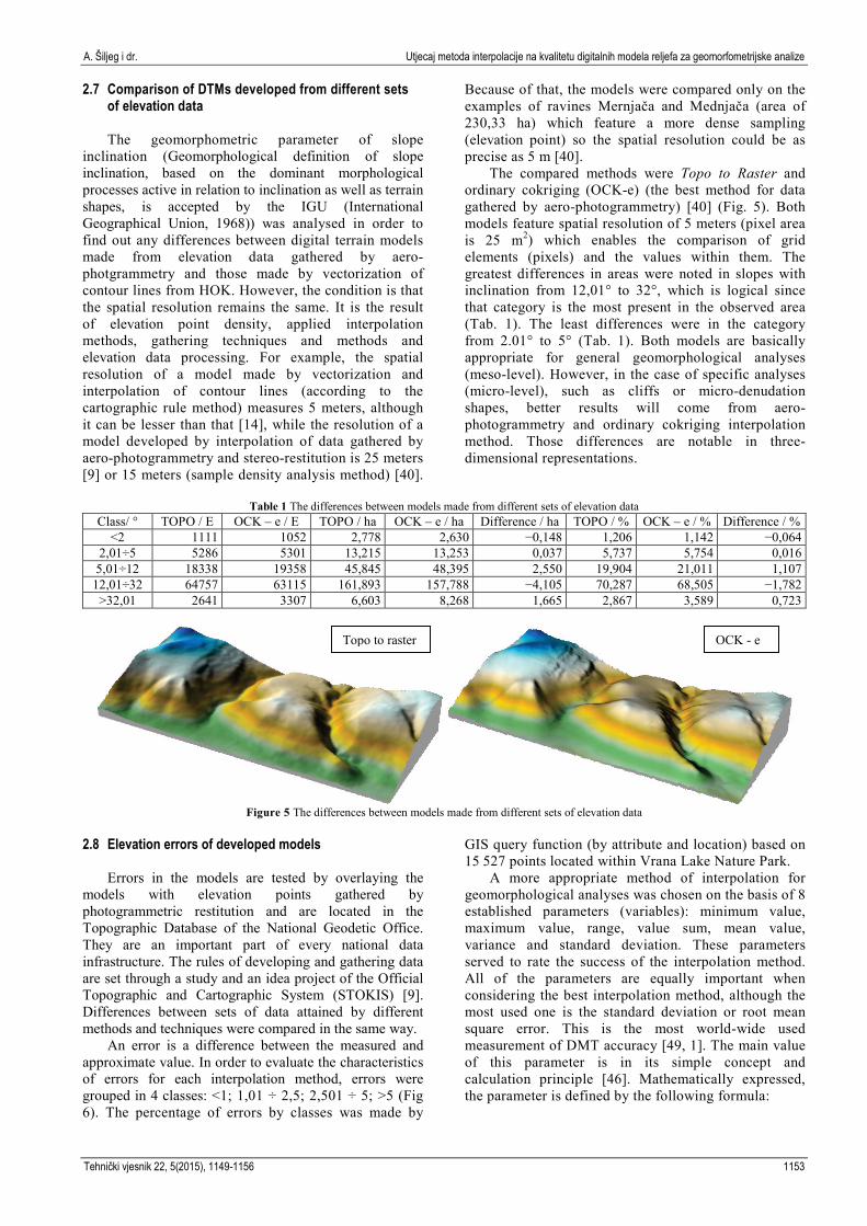
Because of that, the models were compared only on the examples of ravines Mernjača and Mednjača (area of 230,33 ha) which feature a more dense sampling (elevation point) so the spatial resolution could be as precise as 5 m [40].

The compared methods were Topo to Raster and ordinary cokriging (OCK-e) (the best method for data gathered by aero-photogrammetry) [40] (Fig. 5). Both models feature spatial resolution of 5 meters (pixel area is 25 m2) which enables the comparison of grid elements (pixels) and the values within them. The greatest differences in areas were noted in slopes with inclination from 12,01° to 32°, which is logical since that category is the most present in the observed area (Tab. 1). The least differences were in the category from 2.01° to 5° (Tab. 1). Both models are basically appropriate for general geomorphological analyses (meso-level). However, in the case of specific analyses (micro-level), such as cliffs or micro-denudation shapes, better results will come from aero-photogrammetry and ordinary cokriging interpolation method. Those differences are notable in three-dimensional representations.

Table 1 The differences between models made from different sets of elevation data

Class/ ° TOPO / E OCK – e / E TOPO / ha OCK – e / ha Difference / ha TOPO / % OCK – e / % Difference / % <2 1111 1052 2,778 2,630 −0,148 1,206 1,142 −0,064

2,01÷5 5286 5301 13,215 13,253 0,037 5,737 5,754 0,016 5,01÷12 18338 19358 45,845 48,395 2,550 19,904 21,011 1,107

12,01÷32 64757 63115 161,893 157,788 −4,105 70,287 68,505 −1,782 >32,01 2641 3307 6,603 8,268 1,665 2,867 3,589 0,723

Figure 5 The differences between models made from different sets of elevation data

2.8 Elevation errors of developed models

Errors in the models are tested by overlaying the models with elevation points gathered by photogrammetric restitution and are located in the Topographic Database of the National Geodetic Office. They are an important part of every national data infrastructure. The rules of developing and gathering data are set through a study and an idea project of the Official Topographic and Cartographic System (STOKIS) [9]. Differences between sets of data attained by different methods and techniques were compared in the same way.

An error is a difference between the measured and approximate value. In order to evaluate the characteristics of errors for each interpolation method, errors were grouped in 4 classes: <1; 1,01 ÷ 2,5; 2,501 ÷ 5; >5 (Fig 6). The percentage of errors by classes was made by

GIS query function (by attribute and location) based on 15.527 points located within Vrana Lake Nature Park.

A more appropriate method of interpolation for geomorphological analyses was chosen on the basis of 8 established parameters (variables): minimum value, maximum value, range, value sum, mean value, variance and standard deviation. These parameters served to rate the success of the interpolation method. All of the parameters are equally important when considering the best interpolation method, although the most used one is the standard deviation or root mean square error. This is the most world-wide used measurement of DMT accuracy [49, 1]. The main value of this parameter is in its simple concept and calculation principle [46]. Mathematically expressed, the parameter is defined by the following formula:

Topo to raster OCK - e



{ } ,)()(12

1∑=

−=N

iji xzxz

NRMSE (4)

where: xi − approximate value on the location i; z(xi) − measured (real) value on the location i; N − number of measured points.

Root mean square error expresses the level at which the interpolated values differ from the measured ones. It is based on the assumption that the accidental errors average 0 and that they are normally distributed [8]. Most of the papers dealing with that subject found out that the root mean square error is not 0 [41, 36, 35, 36]. In ANUDEM interpolation method, 54,338 % of the points have an error smaller than 1 meter (Tab. 2). Root mean square error is 1,859 meters, while the maximum error is

−12,078 (Tab. 3). Standard deviation in TIN method is 1,876 meters, whereas maximum one is −17,546 meters (Tab. 3). The percentage of errors within 1 meter in TIN method is 53,107 %. The highest percentage of errors >5,01 meters was present in the vertically dissected part of Vrana Lake Natural Park or Mernjača and Mednjača ravines, for both methods (approximately 2 %) (Tab. 2; Fig. 6).

Table 2 The number and percentage of elevation errors by classes Classes TOPO % TIN %

< 1 8437 54,338 8246 53,107 1,01 ÷ 2,5 4992 32,150 5104 32,872 2,501 ÷ 5 1705 10,981 1806 11,631

> 5,01 393 2,531 371 2,389

Table 3 Differences between measured and approximate values

IM Number of points

Min. value/ m

Max. value/ m Range/ m Value sum/ m Mean value /

m Variance/ m² Standard deviation / m

ANUDEM 15.527 −12,078 11,351 23,429 2227,853 0,143 1,363 1,859 TIN 15.527 −17,546 12,169 29,715 418,396 0,027 1,370 1,876

Figure 6 Pictogram of elevation errors by classes

3 Discussion

The results of this research showed that the output results of digital models depend on the data gathering methods, sample density, interpolation methods, terrain features (primarily vertical dissection) and pixel size. The main aim of this paper was to determine the most appropriate method of interpolation and spatial resolution for purposes of various geomorphological researches. From the five most common methods of gathering elevation data and comparison of digital interpolation models, two sets of elevation data were used. They were obtained by different methods, techniques and procedures

of data gathering: aero-photogrammetry, stereo-restitution and vectorization of contour lines from HOK.

Two methods of interpolation of contour lines were compared: TIN and ANUDEM (Topo to raster). The observed methods showed significant differences in generating surfaces, especially on flat terrain. The differences are most obvious when deriving geomorphometric parameters from those models. Topo to raster method showed better results and is more appropriate for developing models and analyses used by geomorphometric researches. The model that was developed by Topo to raster method was compared (by analysing geomorphometric parameter of slope inclination) to the best model developed by aero-



photogrammetrically gathered data. The research showed that there are no significant differences between the observed methods in the context of general geomorphological analyses (at a meso-level). However, when performing specific analyses (micro-level), such as on cliffs or micro-denudation formations, the results were better in the case of aero-photogrammetrically gathered data and interpolated by ordinary cokriging method. Those differences were notable on the developed three-dimensional representations.

Most of the authors who have researched a similar subject offer information only about root mean square error of the developed models. However, there are other errors in those models, such as minimum and maximum errors, that need to be taken into consideration. This research classified elevation errors into four classes in order to determine the characteristics of errors. The effect of vertical dissection of the output data was also determined.

Elevation errors of the developed models were obtained on the basis of 15.527 points gathered by aero-photogrammetry. It is important to note that points obtained by photogrammetry also feature an aspect of error which is a result of stereo-restitution. It is recommended that the future researches employ overlaying the developed models with the elevation points gathered by a precise base GPS. The drawback is that it is quite difficult to determine the exact number of samples in such case.

4 Conclusion

After the analysis of statistical parameters and elevation errors it can be concluded that there are no significant differences between the two methods, especially in terms of standard deviation (the difference being only 1,7 cm). Such results were not expected, since the interpolation functions were different. The reason behind such result is most probably a large number of samples that were used for checking the accuracy of the developed models. The differences between the models are most evident when they are used to derive the morphometric parameter of slope inclination. 5 References [1] Aguilar, F. J.; Agüera, F.; Aguilar, M. A.; Carvajal, F.

Effects of terrain morphology, sampling density, and interpolation methods on grid DEM accuracy. // Photogrammetric Engineering and Remote Sensing. 71, 7(2005), pp. 805-816. DOI: 10.14358/PERS.71.7.805

[2] Ali, T. A. On the selection of an interpolation method for creating a terrain model (TM) from LIDAR data. // American Congress on Surveying and Mapping (ACSM) Conference 2004: Proceedings / Nashville TN, USA, 2004.

[3] Biljecki, Z.; Tonković, T.; Franić S. Studija o nadomještanju reprodukcijskih izvornika i obnavljanju sadržaja topografskih zemljovida. Geofoto d.o.o., Zagreb, 1995.

[4] Burrough, P. A.; McDonnell, R. A. Principles of Geographical Information Systems. Oxford University Press, New York, 1998.

[5] Cetl, V.; Tutić, D. Automated vectorization in cadastre. // Geodetski list. 56, 2(2002), pp. 103-116.

[6] Cheveresan, B. Digital Terrain Model Accuracy for Flooded Area Delineation. 2012. http://balwois.com/2012/ USB/papers/523.pdf (29.10.2012).

[7] Childs, C. Interpolating Surfaces in ArcGIS Spatial Analyst. // ESRI Education Services. 2004. http://webapps.fundp.ac.be/geotp/SIG/interpolating.pdf (12.5.2012)

[8] Desmet, P. J. J. Effects of interpolation errors on the analysis of DEMs. //Earth Surface Processes and Landforms. 22, 6 (1997), pp. 563-580. DOI: 10.1002/(SICI)1096-9837(199706)22:6<563::AID-ESP713>3.0.CO;2-3

[9] DGU.Product specification: Digital elevation model. CRONO GIP, Zagreb, 2003.

[10] Erdogan, S. A comparison of interpolation methods for producing digital elevation models at the field scale. // Earth Surface Processes and Landforms. 34, 3(2009), pp. 366-376. DOI: 10.1002/esp.1731

[11] Frančula, N. Digitalna kartografija (Digital Cartography). Geodetski fakultet, Sveučilište u Zagrebu, Zagreb, 2004.

[12] Gjuranić, Ž. Modeliranje terena pomoću Delaunayjeve triangulacije (Terrain Modelling by Using Delaunay Triangulation). // KoG.11(2008), pp. 49-52.

[13] Goodchild, M. F.; Mark, D. M. The fractal nature of geographic phenomena. // Annals of Association of American Geographers. 77, 2(1987), pp. 265-278. DOI: 10.1111/j.1467-8306.1987.tb00158.x

[14] Hengel, T. Finding the right pixel size. //Computer and Geosciences. 32, 9(2006), 1283-1298. DOI: 10.1016/j.cageo.2005.11.008

[15] Hengel, T. A Practical Guide to Geostatistical Mapping of Environmental Variables. European Communities, JRC Scientific and Technical Report, Luxembourg, 2007.

[16] Hengl, T.; Gruber, S.; Shrestha, D. P. Digital terrain analysis in ILWIS: lecture notes and user guide. International Institute for Geo-information Science and Earth Observation (ITC), Enschede, Netherlands, 2003.

[17] Horvat, S.; Železnjak, Ž.; Lapaine, M. Military Topographic and Cartographic System of the Republic of Croatia. // KIG. 2(2003), pp. 75-85.

[18] Hu, K.; Li, B., Lu, Y.; Zhang, F. Comparison of various spatial interpolation methods for non-stationary regional soil mercury content. // Environmental Science. 25, 3(2004), pp. 132-137.

[19] Hutchinson, M. F.A new procedure for gridding elevation and stream line data with automatic removal of spurious pits. // Journal of Hydrology. 106 (1989), pp.211-232. DOI: 10.1016/0022-1694(89)90073-5

[20] Hutchinson, M. F. A locally adaptive approach to the interpolation of digital elevation models. //Proceedings of the Third International Conference/Workshop on Integrating GIS and Environmental Modeling/Santa Barbara, CA, 1996.

[21] IGU, Commission on applied geomorphology, subcommission on geomorphological mapping. The unified key to the detailed geomorphologial map of the world, 1: 25000 – 1: 50000. // Folia geografica, Series geographica-physica. 2(1968)

[22] Johnston, K.; Hoef, J. M. V.; Krivoruchko, K., Lucas, N. Using ArcGISTM Geostatistical Analyst. ESRI, Redlands, USA, 2001.

[23] Kenny, F.; Matthews, B. A methodology for aligning raster flow direction data with photogrammetrically mapped hydrology. // Computers & Geosciences. 31, 6(2005), pp. 768-779. DOI: 10.1016/j.cageo.2005.01.019

[24] Li, Z.; Zhu, Q.; Gold, C. Digital Terrain Modeling. CRC Press, London, 2005.

[25] Miller, C.; Laflamme, R. The digital terrain model - theory and applications. // Photogrammetric Engineering. 24(1958), pp. 433-442.



[26] Mitas, L.; Mitasova, H. Spatial Interpolation // Geographical Information Systems: Principles, Techniques, Management and Applications (Second edition) (Eds.: Longley, P.; Goodchild, M. F.; Maguire, D. J.; Rhind, D. W.), Wiley, Chichester, 1999, pp. 481-492.

[27] Moore, I. D.; Grayson, R. B.; Ladson, A. R. Digital terrain modelling: a review of hydrological, geomorphological, and biological applications. // Hydrological Processes. 5(1991), pp. 3-30. DOI: 10.1002/hyp.3360050103

[28] Naoum, S.; Tsanis, I. K. Ranking spatial interpolation techniques using a GIS-based DSS. //Global Nest: the International Journal. 6, 1(2004), pp. 1-20.

[29] Pebesma, E. J. Multivariable geostatistics in S: the Gstat package. // Computer & Geosciences. 30, 7(2004), pp. 683-691. DOI: 10.1016/j.cageo.2004.03.012

[30] Peralvo, M. Influence of DEM interpolation methods in drainage analysis. // Gis Hydro 04, University of Texas, Austin, 2004. http://www.crwr.utexas.edu/gis/gishydro04/ introduction/termprojects/peralvo.pdf (29.10. 2012).

[31] Pike, R. J. Geomorphometry - progress, practice and prospect. // Zeitschrift für Geomorphologie. Supplementband. 101 (1995), pp. 221-238.

[32] Pike, R. J. Geomorphometry - diversity in quantitative surface analysis. // Progress in Physical Geography. 24, 1(2000), pp. 1-20.

[33] Radoš, D.; Lozić, S.; Šiljeg, A. Morphometrical characteristics of the broader area of Duvanjsko polje, Bosnia and Herzegovina. // Geoadria. 17, 2(2012), pp. 177-207.

[34] Radoš, D.; Lozić, S.; Šiljeg; A., Jurišić, M. Features of Slope Inclination and Planar Curvatures of the broader Area of Duvanjsko polje. // Geodetski list. 4(2012), pp. 273-301.

[35] Ripley, B. D. Spatial Statistics. John Wiley & Sons, New York, 1981. DOI: 10.1002/0471725218

[36] Sheikhhasan, H. A Comparison of Interpolation Techniques for Spatial Data Prediction.Master’s Thesis in Computer Science. Faculty of Science, Universiteit van Amsterdam, The Netherlands, 2006.

[37] Smith, S. L.; Holland, D. A.; Longley, P. A. Quantifying interpolationerrors in urban airborne laser scanning models. // Geographical Analysis. 37, 2(2005), pp. 200-224. DOI: 10.1111/j.1538-4632.2005.00636.x

[38] Soenario, I.; Plieger, M.; Sluiter, R.Optimization of Rainfall Interpolation. Royal Netherlands Meteorological Institute (KNMI), De Bilt, Nederlands, 2010.

[39] Svobodava, J. Selection of Appropriate Interpolation Methods for Creation DEMs of Various Types of Relief by Copplex Approach to Assessment of DEMs. // GIS Ostrava, (2011), http://gis.vsb.cz/GIS_Ostrava/GIS_Ova_2011/ sbornik/ papers/Svobodova.pdf (02.10.2012.)

[40] Šiljeg, A. Digital Terrain Model in the Analysis of Geomorphometrical Parameters - The Example of Nature Park Lake Vrana). Doctoral Thesis. Faculty of Science, University of Zagreb, 2013. 187 p.

[41] Tomczak, M. Spatial Interpolation and its Uncertainty Using Automated Anisotropic Inverse Distance Weighting (IDW) - Cross-Validation/Jackknife Approach. // Journal of Geographic Information and Decision Analysis. 2, 2(1998), pp. 18-30.

[42] Wahba, G. Spline models for Observational data. Soc. Ind. Appl. Maths., Philadelphia, 1990. DOI: 10.1137/1.9781611970128

[43] Watson, D. F. Contouring: A Guide to the Analys is and Display of Spatial Data. Pergamon Press, Oxford, UK, 1992.

[44] Webster, R.; Oliver, M. A.Geostatistics for Environmental Scientists. John Wiley & Sons Ltd, Chichester, 2007. DOI: 10.1002/9780470517277

[45] Weibel, R.; Heller, M. Digital terrain modelling. // Geographical Information Systems: Principles and Applications, Vol. 1: Principles (Eds: Maguire, D. J., Goodchild, M. F., Rhind, D.), Longman, Harlow, 1991.

[46] Weng, Q. An evaluation of spatial interpolation accuracy of elevation data. // Progress in Spatial Data Handling (Eds. Riedl, A., Kainz, W., Elmes, G. A.), Springer-Verlag, Berlin, 2006. pp. 805-824.

[47] Wilson, J. P.; Gallant, J. C. Digital terrain analysis. // Terrain analysis: principles and applications (Eds. Wilson, J. P, Gallant, J. C.), John Wiley and Sons: New York, 2000, pp. 1-27.

[48] Yang, C. S.; Kao, S. P.; Lee, F. B.; Hung, P. S. Twelve Different Interpolation Methods: a Case Study of Surfer 8.0. // Proceedings of the XXth ISPRS Congress, Istanbul, 2004, pp. 778-783.

[49] Yang, X.; Hodler, T. Visual and statistical comparisons of surface modeling techniques for point-based environmental data. // Cartography and Geographic Information Science. 27, 2(2000), pp. 165-175. DOI: 10.1559/152304000783547911

[50] Yang, Q. K.; McVicar, T. R.; Van Niel, T. G.; Hutchinson, M. F.; Li, L. T.; Zhang, X. P. Improving a digital elevation model by reducing source data errors and optimising interpolation algorithm parameters: an example in the Loess Plateau. Chin. // Int. J. Appl. Earth Obs. Geoinf. 9(2007), pp. 235-246. DOI: 10.1016/j.jag.2006.08.004

Authors' addresses Ante Šiljeg, Ph.D. Sveučilište u Zadru, Odjel za geografiju Trg kneza Višeslava 9, 2300 Zadar, Croatia E-mail: [email protected] Sanja Lozić, Ph.D. Assist. Prof. Sveučilište u Zadru Odjel za geografiju Trg kneza Višeslava 9, 2300 Zadar, Croatia E-mail: [email protected]; [email protected] Cell: 098/540-832 Denis Radoš, mag. geogr. Sveučilište u Zadru Odjel za geografiju Trg kneza Višeslava 9, 2300 Zadar, Croatia E-mail: [email protected]

the effect of interpolation methods on the …

Documents