IZA DP No. 3696

The Effect of High School Employment onEducational Attainment: A ConditionalDifference-in-Differences Approach

Franz BuschaArnaud MaurelLionel PageStefan Speckesser

DI

SC

US

SI

ON

PA

PE

R S

ER

IE

S

Forschungsinstitutzur Zukunft der ArbeitInstitute for the Studyof Labor

September 2008

The Effect of High School Employment on

Educational Attainment: A Conditional Difference-in-Differences Approach

Franz Buscha University of Westminster

Arnaud Maurel

CREST-ENSAE, Paris School of Economics and IZA

Lionel Page University of Westminster

Stefan Speckesser

University of Westminster

Discussion Paper No. 3696 September 2008

IZA

P.O. Box 7240 53072 Bonn

Germany

Phone: +49-228-3894-0 Fax: +49-228-3894-180

E-mail: iza@iza.org

Any opinions expressed here are those of the author(s) and not those of IZA. Research published in this series may include views on policy, but the institute itself takes no institutional policy positions. The Institute for the Study of Labor (IZA) in Bonn is a local and virtual international research center and a place of communication between science, politics and business. IZA is an independent nonprofit organization supported by Deutsche Post World Net. The center is associated with the University of Bonn and offers a stimulating research environment through its international network, workshops and conferences, data service, project support, research visits and doctoral program. IZA engages in (i) original and internationally competitive research in all fields of labor economics, (ii) development of policy concepts, and (iii) dissemination of research results and concepts to the interested public. IZA Discussion Papers often represent preliminary work and are circulated to encourage discussion. Citation of such a paper should account for its provisional character. A revised version may be available directly from the author.

IZA Discussion Paper No. 3696 September 2008

ABSTRACT

The Effect of High School Employment on Educational Attainment: A Conditional Difference-in-Differences Approach*

Using American panel data from the National Educational Longitudinal Study of 1988 (NELS:88) this paper investigates the effect of working during grade 12 on attainment. We exploit the longitudinal nature of the NELS by employing, for the first time in the related literature, a semiparametric propensity score matching approach combined with difference-in- differences. This identification strategy allows us to address in a flexible way selection on both observables and unobservables associated with part-time work decisions. Once such factors are controlled for, insignificant effects on reading and math scores are found. We show that these results are robust to a matching approach combined with difference-in-difference-in-differences which allows differential time trends in attainment according to the working status in grade 12. JEL Classification: J24, J22, I21 Keywords: education, evaluation, propensity score matching Corresponding author: Arnaud Maurel ENSAE -Timbre J120 3, Avenue Pierre Larousse 92245 Malakoff cedex France E-mail: maurel@ensae.fr

* We thank Magali Beffy, Pierre-Philippe Combes, Juan José Dolado, Denis Fougère, Marc Gurgand, Xavier d'Haultfoeuille, Cecilia Garcia Penalosa, Fabien Postel-Vinay and participants at the European Society for Population Economics congress 2008, the European Association of Labour Economics conference in 2007, the Association Française de Science Economique conference in 2007 and the GREQAM Spring Graduate School in Economics - Recent Advances in Labour Economics (Aix-en-provence, France) in 2007 for helpful comments and discussion.

1 Introduction

There has, in recent years, been an upsurge in the number of studies examining the effects

of working part-time while studying. This employment effect is typically considered with

respect to educational outcomes, but also with respect to post-school wages and employment

probabilities. Some authors, such as Warren, LePore and Mare (2000), argue that studies have

typically treated educational careers and occupational careers as mutually exclusive and that

only recently attention has been garnered toward examining the relationship between students

who work and their educational achievements. Such research suggests that there is a high level

of interaction between earning and learning. Nonetheless, whilst it is true that the subject of

working during school hours is gaining popularity in the literature, the phenomenon of working

during education has been known for some time to both sociologists and economists.

It has now been over two decades since both D’Amico (1984) and Michael and Tuma (1984)

observed that employment among young people in the education system is remarkably high.

Michael and Tuma remark that: “Among 14- and 15- year-old students in 1979, about one

in four was employed [and that] this is not a trivial rate of employment” (p. 466). Likewise

D’Amico noted that employment intensity increases rapidly as age progresses, from approxi-

mately 40 percent for those in grade 10 to 70 percent for those in grade 12. It was here that

some of the first questions about the effect of working during school on attainment were raised.

Such questions are primarily concerned with whether working during schooling can be seen

as a substitute or as a complement to education. Part-time work can be seen as a substitute to

education because any additional increase in time spent working lead, ceteris paribus, to a

reduction in time spent on education1. This, in turn, might negatively affect any educational

outcomes. Alternatively, it may be that working complements educational attainment via the

acquisition of a variety of skills such as improved work values, literacy and numeracy skills.

If one assumes that such skills are general and transferable, it is possible that individuals who

work whilst in full-time education might have a learning advantage compared to those who do

1This argument is usually referred to in the literature as the zero-sum model.

2

not (Holland and Andre, 1987).

Most of the existing studies show that working particularly long hours during school has

a detrimental impact on educational attainment. However, there is also evidence from the lit-

erature that working a small amount of hours may be beneficial to studying. Working during

school can thus both be a complement or a substitute to education, depending on the amount of

hours worked.

On an empirical ground, the main difficulty in identifying and thus estimating the causal

effect of part-time work on educational attainment lies in the potential endogeneity of part-

time work. Indeed, labour supply decisions of students are likely to be related to unobserved

characteristics that are in turn related to academic attainment. For instance, conditional on

observables, students deciding to work part-time may have a lower unobserved ability or moti-

vation for schooling. In that case, OLS estimates would lead to overstate the detrimental effect

of part-time work.

The endogeneity issue has cast doubt on earlier obtained results, and has led to the imple-

mentation of instrumental variable estimators (Ehrenberg and Sherman, 1987; Lillydahl, 1990;

Singh, 1998; Warren, LePore and Mare, 2000; Tyler, 2003; Stinebrickner and Stinebrickner,

2003; Dustmann and van Soest, 2007; Rothstein, 2007). However, as already pointed out by

Stinebrickner and Stinebrickner (2003), an instrument causing an exogenous variation of part-

time work decisions is very difficult to find in this context. Up to now, even the best attempts to

provide such an exogenous variation are questionable. Using U.S. interstate variations in child

labour laws as an instrument for students labour supply as it is done by Tyler(2003) might not

be valid, since the adoption of specific child labour laws within a state might be related among

others to the emphasis placed on educational attainment2 and therefore be also endogenous with

respect to academic attainment.

In this paper, relying on the National Educational Longitudinal Study of 1988 (NELS:88)

dataset, we address such issue using nonexperimental estimators which do not rely on the va-

2Given the widely spread belief of an adverse impact of part-time work on educational attainment, it might bethat a state placing greater emphasis on academic attainment would adopt more stringent child labor laws.

3

lidity of an instrument in order to estimate the causal effect of part-time work during grade 12

on educational attainment. We take advantage of both the longitudinal nature of the NELS and

the richness of the available set of covariates by employing, for the first time in the related em-

pirical literature, a semiparametric local linear matching approach combined with difference-

in-differences (conditional difference-in-differences, CDiD, Heckman, Ichimura, Smith and

Todd, 1998). This identification strategy allows us to address selection on both observables and

unobservables associated with labour supply decisions of students. A closely related method-

ological approach has recently been followed on the same dataset by Sanz-de-Galdeano and

Vuri (2007) which uses a DiD estimator to assess the effect of divorce on students’ academic

performances. Our identification strategy differs from theirs in the extent that it relies on a more

flexible semiparametric matching approach in order to control for the observable characteristics

of the individuals.

Once observable and unobservable factors are controlled for, we find negligibly small ef-

fects on twelfth grade standardized reading and math scores, even for intensive part-time em-

ployment. Comparison with OLS estimates suggests that any negative relationship between

part-time work and educational attainment is actually due to unobservable effects.

The remainder of this paper is set out as follows. In section 2 we briefly present stylized

facts about part-time work during schooling in the United States. Section 3 will highlight the

zero-sum model, how it relates to the effect of part-time work on educational attainment and

provide an overview of previous findings in the literature. Section 4 outlines a theoretical model

of the decision to work part-time. Section 5 provides a brief overview of the National Educa-

tion Longitudinal Study of 1988 (NELS:88) and its associated descriptive statistics. Section 6

details the empirical analysis while section 7 presents the results. Finally section 8 concludes.

4

2 Youth employment during schooling in the United States

It should be remembered that whilst the minimum school-leaving age in the United States is at

age 16, the minimum legal working age is age 14 or above.3 Even those below the minimum

legal working age may find part-time employment in informal jobs such as babysitting or deliv-

ering newspapers. This implies that a substantial part of the schooling population is eligible to

perform some function in the labour market, and therefore, one cannot separate the education

and the labour market completely.

The Youth Labor Force 2000 report, by the American Bureau of Labor Statistics, finds

that during the 1996-1998 period 2.9 million 15 to 17 year olds worked during school months,

while during the summer months this increased to 4 million. It appears that the prevalence

of part-time work increases with age and “at age 12, half of the American youths engage in

some type of work activity” (p. 20). This number increases to over half (57%) for 14 year olds

and to 64% for those aged 15. By age 16 to 17 over 80 percent of individuals will have held

a part-time job. Furthermore, as age progresses the nature of work appears to formalise from

freelance work into a more mature and binding employment relationship. Evidence from the

literature finds likewise proportions, and of those who do work, the work intensity is substantial

and increasing with age (Ruhm, 1995). Besides, as mentioned by Singh (1998), the proportion

of students holding a part-time job has dramatically increased during the last decades since

students in the 1990s were twice as likely to work part-time as students in 1950.

It should also be noted that within the policy environment a dichotomy of views exist. Those

holding the view that working is complementary for educational experiences of young adults

are in favor of formal school-to-work programmes, with the aim of expanding the employment

experience of students. Conversely, those who hold a less favorable view and argue that such

programmes are undesirable and counter-productive consider that more stringent child labour

laws should be considered (Warren, 2002). Noteworthy is that the conviction of a detrimental

effect of part-time work on educational attainment, relying on academic research, is increas-

3Note that state-wise variations exist for both the minimum school leaving age and the minimum working age.

5

ingly wide-spread since last ten years. This view has recently led some states, such as Mas-

sachusetts or Colorado, to implement more stringent child labour laws reducing the maximum

amount of time students could work during the school-year.

3 Literature review

In this section, after presenting the baseline zero-sum model which is used in the literature

as a core framework for analyzing the relationship between part-time work and educational

attainment, we will review the related empirical literature.

3.1 Modeling the relationship between part-time work and educational

attainment

The time perspectives of working part-time during education are based on the zero-sum model

(Coleman, 1961; D’Amico, 1984; Marsh; 1991; Warren, 2002), which provides a core theoret-

ical framework for examining the relationship between part-time employment and educational

attainment. The zero-sum model argues that time has a finite horizon and any additional time

spent on employment during education must lead to a reduction in time spent on educational

advancement, ceteris paribus. Additionally, participation in extra-curricular activities which

could improve psychological adjustment and commitment to schooling, may be hampered by

those in part-time employment (Lewin-Epstein, 1981; D’Amico, 1984).

Within this baseline model, individuals are assumed to choose the amount of time devoted

to part-time work (Tpt) and homework (Th) by maximizing their utility, subject to the following

time constraint:

T = Th + Tpt + Tl(1)

Where T denotes the total amount of time available outside of school and Tl the amount of time

allocated to leisure.

6

Throughout the literature examining the effect of part-time work on educational attainment,

the zero-sum model has mainly been used to provide a framework which yields negative returns

to part-time work in terms of educational attainment. Within this framework, negative returns

to part-time work simply stem from the fact that time spent working is taken away from other

activities such as homework, which in turn is assumed to have a positive effect on educational

attainment.

Nevertheless, the zero-sum model is not necessarily incompatible with positive returns to

education from working part-time. Indeed, if one additionally assumes that educational skill

accumulation suffers from diminishing marginal returns and that working part-time during

schooling results in a positive amount of educational skill accumulation (Holland and An-

dre,1987), then the net pay-off to attainment from working few hours per week may be larger

than investing a few hours more on homework per week. In other words, the marginal return of

working during full-time education might be higher than the marginal return of homeworking.

Thus, depending on the assumptions which are made on the attainment production function,

the zero-sum model can be both consistent with a detrimental as well as a positive effect of

part-time work on academic achievement.

3.2 Prior evidence

Over the last twenty years, especially in the United States, much interest and debate has focused

on the effects of working during full-time education. Some of these studies indicated reduced

academic performance by students who worked (Greenberger and Steinberg, 1980; Marsh,

1991; Eckstein and Wolpin, 1999; Tyler, 2003; Stinebrickner and Stinebrickner, 2003), whilst

others found no negative effect (Meyer and Wise, 1982; D’Amico, 1984; Green and Jacques,

1987; Mortimer, Finch, Shanahan, and Ryu, 1992; Schoenhals et al., 1998; Warren et al, 2000;

Rothstein, 2007). Many papers, however, showed that the effects varied, depending on hours

worked - that modest involvement in employment did not interfere with academic performance

and was sometimes associated with a positive impact on grades, but intense involvement had

7

negative effects - (Steinberg et al., 1982; Schill et al., 1985; Lillydahl, 1990; Steel, 1991;

Turner, 1994; Cheng, 1995; Singh, 1998; Oettinger, 1999; Montmarquette et al., 2007). This

appears to be the most predominant finding in the literature with an approximate inflection

point varying between 10-20 hours of work per week.

Early empirical research into the effects of working whilst in education was first conducted

by Steinberg et al (1982), Steinberg and Greenberger (1980) and Greenberger et al (1980).

More rigorous statistical analysis is introduced by D’Amico (1984) who uses OLS estimation

to find that working part-time does not appear to have a detrimental effect on educational attain-

ment. Marsh (1991), however, using High School and Beyond daya (HSB) finds a linear and

negative relationship between work and test scores whilst Mortimer et al (1992) conclude that

twelfth graders working less than 20 hours had significantly higher grades compared to those

who worked 20 hours or more. Similar findings are produced by Steinberg et al (1982) and

Worley (1995) who argue that the number of hours worked per week has a significant negative

impact on educational attainment.

It should be noted that some findings suggest that working few hours may be beneficial

to educational attainment (D’Amico, 1984; Schill et al, 1985; Steel, 1991; Turner, 1994).

These studies find that pupils working few hours per week are likely to have higher educational

achievement compared to those who work long hours or no hours at all. However, an essential

problem with the above findings is their failure to take into account the potential endogeneity

of working part-time during schooling.

In one of the first papers to address such issue, Ehrenberg and Sherman (1987) acknowledge

the issue of endogeneity and argue that “[the previous literature] is not completely satisfactory

in that it fails to control for the possibilities that such employment is determined simultaneously

with choice of college...” (p. 2). Using an IV approach they find that there does not appear to be

an adverse effect on grade point average from working part-time during college, though there

is a significant adverse effect on the probability of staying-on in education. Lilydahl’s (1990)

study, using the 1987 National Assessment of Economic Education Survey was another early

adopter of two-stage least squares approach, also arguing that part-time work and educational

8

attainment were likely to be simultaneously determined. Evidence by Ruhm (1997) suggests

that OLS estimates are likely to understate any effects of working part-time during schooling.

Relying on selection methods, he notes that the Mills coefficient in his equations is positive and

significant indicating that selection bias is taking place. Recent work by Eckstein and Wolpin

(1999), Stinebrickner and Stinebrickner (2003), Dustman and van Soest (2007), Montmarquette

et al. (2007) and Rothstein (2007) continue to highlight the importance to take endogeneity into

account in order to recover the causal effect of part-work on educational attainment.

A number of previous papers also rely on the NELS:88 dataset to analyse the impact work-

ing part-time has on educational attainment. Singh (1998), using a structural equation approach,

finds that working in grade 10 has a small detrimental effect on achievement in English, Read-

ing and Social Science when gender, socioeconomic status and previous attainment are con-

trolled for. Schoenhals, Tienda and Schneider (1998) also examine tenth grade achievement

using OLS regression, and argue that the much cited adverse effect of working part-time during

school on educational attainment is actually “(...)attributable to pre-existing differences among

youth who elect to work at various intensities”. Once such observable differences are taken

into account any significant impact on educational attainment from working disappears. War-

ren, Lepore and Mare (2000) also find little evidence that there is a relationship between long

or short term grades from working whilst in high-school.

Finally, Tyler (2003), also relying on the same dataset, finds opposite results compared to

the three previous studies. Using interstate variations in child labour laws as an instrument for

students’ labour supply, he finds significant effects of part-time work on twelfth grade achieve-

ment and argues that OLS estimates severely underestimate the negative impact of working

part-time during schooling. His OLS results indicate that decreasing student work by 10 hours

per week would increase twelfth grade maths score by 0.03 of a standard deviation, for IV es-

timates this increases to 0.20 of standard deviation. Tyler concludes that if government policy

is to raise education standards, more restrictive child labour laws for individuals aged 16-17

ought to be considered.

Whilst we have only surveyed part of the literature it should be clear that the debate about

9

the impact of working part-time during schooling on educational attainment is complex and

still not settled. Methodological advances such as sample selection procedures, IV estimation

and simultaneous equation modeling have meant that the validity of some of the earlier results

has been put to question. Furthermore, even the arguably most robust attempts to address the

endogeneity of part-time work decisions might not be valid. That is even the case of local

child labour laws, since they can be related to state-specific unobserved characteristics directly

affecting students’ achievement, such as school and teaching quality. The main contribution of

our paper lies in the identification strategy we rely on, which does not need to instrument part-

time work decisions. Relying on the longitudinal nature of the NELS we employ, as proposed

by Heckman, Ichimura, Smith and Todd (1998), a semiparametric matching approach combined

with difference-in-differences in order to estimate the effect of part-time work during grade 12

on educational attainment. Such an identification strategy allows us to address in a flexible way

selection on both observables and unobservables associated with part-time work decisions in

order to estimate the causal effect of part-time work on achievement.

4 The model

In this section, we present a simple model in which educational attainment as well as part-time

work and the amount of time devoted to homework during high school are endogenous. This

theoretical framework enables to rationalize our reduced-form empirical strategy that will be

exposed later.

In the model, we assume that the student values his consumption C (throughout the aca-

demic year), his twelfth grade attainment S and time allocated to leisure Tl. Denoting by V

the value function of the student and by V the component which is constant with respect to the

choice variables, we have:

V = V (Tl, S, C) + V(2)

10

Note that the model supposes that students gain utility from the educational attainment it-

self. This specification is consistent with the Beckerian view, as it may result from expected

lifetime earnings: a higher achievement during twelfth grade leads to an expectation of getting

a higher degree, resulting therefore in higher expected earnings throughout lifetime. That may

also stem from the social gratification directly resulting from academic achievement (consump-

tion value of schooling).

When entering twelfth grade, the student is assumed to choose simultaneously the amount

of time allocated respectively to part-time work (Tpt) and homework (Th). Assuming that the

total amount of time available outside of school (T ) is the same for all students, the time con-

straint can be written as follows:

T = Th + Tpt + Tl(3)

The student rationally chooses the amount of time that he desires to devote to part-time

work (T ∗pt) and homework (T ∗h ), maximizing his value function :

(T ∗pt, T∗h ) = arg max

(Tpt,Th)V(4)

More precisely, as time allocated respectively to part-time work and homework are left-censored,

T ∗pt and T ∗h defined above can be seen as latent variables underlying Tobit models4. Assuming

the labour market is in equilibrium, the actual amount of time allocated by the student to part-

time work (Tpt) and homework (Th) satisfy :

Tpt =

T∗pt if T ∗pt > 0

0 otherwise

4The latent variables T ∗pt and T ∗

h can be respectively interpreted as the propensity to work part-time and tospend time doing homework.

11

Th =

T∗h if T ∗h > 0

0 otherwise

Attainment S during twelfth grade is assumed to result from an attainment production func-

tion Π which positively depends on ability a, educational aspiration asp, time devoted to home-

work Th, labour supply Tpt and unobserved individual heterogeneity ε in terms of academic

achievement :

S = Π(a, asp, Th, Tpt, ε)(5)

Therefore, we allow part-time work to have both an indirect negative effect (via the time con-

straint which implies that any additional time spent working while studying must lead ceteris

paribus to a reduction in the amount of time devoted to homework) and a direct positive effect

on attainment. The latter effect may result from skill accumulation : along with Holland and

Andre (1987), part-time working can lead to an acquisition in academically related skills and

knowledge, as well as desirable traits such as responsibility and maturity. Consequently, within

this framework, the impact of part-time work on academic achievement is ambiguous, since we

have:∂S

∂Tpt

=∂Π

∂Tpt

− ∂Π

∂Th

Where ∂Π∂Tpt

and ∂Π∂Th

are assumed to be positive.

Along with its effect on time allocation and attainment, part-time work also leads to a higher

level of consumption. The budget constraint faced by the twelfth grade student can be written

as :

pC = y + ωTpt(6)

Where p denotes the price of consumer good, y the parental financial transfer (net of tuition

12

fees) received by the student and ω the hourly wage earned when participating to the labour

market5

Hence, consumption is positively affected by part-time work :

C =y + ωTpt

p(7)

It stems from the individual program that the amount of time devoted to part-time work

(Tpt) and homework (Th) are functions of the following arguments :

Tpt = Tpt(a, asp, y, ε)(8)

Th = Th(a, asp, y, ε)(9)

Finally, the model can be used to derive a binary part-time work decision :

Part-time work during twelfth grade ⇔ T ∗pt(a, asp, y, ε) > 0(10)

This binary choice is the object of the Probit model which is estimated in the empirical section.6

Note that this framework can also be used to take into account non linearities in the effect of

part-time work on educational attainment, as we can write :

Part-time work (more than k hours) ⇔ T ∗pt(a, asp, y, ε) > k(11)

Therefore, the model allows part-time work decisions to differ among students depending

on schooling ability, educational aspiration, parental financial transfer and unobserved indi-

vidual heterogeneity. Hence, observable factors such as standardized test scores, educational

aspirations, parental income and number of siblings taken as a proxy for parental financial

transfers will be included in the following estimations of part-time work decisions. Selection

5We assume that ω is constant among twelfth graders.6The latent variable underlying the Probit model can be interpreted as the propensity to work part-time.

13

on unobservables will be addressed by considering for each individual the difference in test

scores between grade 10 and grade 12, and then forming the difference between the treatment

(students working part-time during grade 12) and control (those not working during grade 12)

groups.

5 Data and descriptive statistics

The data used in this study are from the National Educational Longitudinal Study of 1988

(NELS:88) conducted by the U.S. National Center for Education Statistics. It is a nationally

representative sample of students who were eight graders in the base year of 1988. Further

follow up surveys were conducted in 1990 (tenth grade), 1992 (twelfth grade), 1994 and 2000,

giving a total of 5 waves. Making use of the “public use file 88/92” we have a total set of 27,394

cases. However, after restricting our analysis to those who are eligible and still in school by

grade 12 we are left with 16,663 observations. Missing values for gender reduce this to 15,747

and finally, dropping missing values for part-time work and test scores leaves us with 9,887

individuals.

The NELS:88 dataset contains a large amount of information about the students, their social

background, their relatives and friends, the characteristics of their school, their success at school

and their way of life. The longitudinal nature of the dataset gives a good opportunity to track

the behaviour of pupils and their success later on. Of special interest in our study is the fact that

the first three waves of the survey include standardized test scores in four disciplines: Maths,

Sciences, History and Reading. These tests were taken at the time of the interview and make

it possible to follow the progression of students across time. Their standardization makes them

comparable both in the time and in the cross section dimensions. The dependent variables

for educational attainment in this study are the composite scores of Mathematics and Reading

tests7. This choice is motivated by the synthetic nature of this index which is likely to take into

7The composite score for reading is based on three different reading tests and for mathematics on five differentmathematics tests.

14

Males FemalesFrequency Percent Frequency Percent

Grade 8Not Working 1,401 29.63 2,594 32.96Working 0 to 10 hours 2,617 55.35 4,558 57.92Working 11 to 20 hours 389 8.23 457 5.81Working 21 or more hours 321 6.79 159 3.08Grade 10Not Working 1,817 38.43 2,563 49.68Working 0 to 10 hours 904 19.12 1,015 19.67Working 11 or more hours 899 19.01 858 16.63Working 21 or more hours 1,108 23.43 723 14.01Grade 12Not Working 1,649 34.88 1,649 31.96Working 0 to 10 hours 764 16.16 981 19.02Working 11 or more hours 1,222 25.44 1,645 31.89Working 21 or more hours 1,093 24.39 884 17.14Total 4,728 100 5,159 100

Table 1: Sample proportions of the incidence of work for grades 8, 10 and 12

account the different ability required from the pupils to succeed in high school.

Furthermore, the NELS:88 survey has detailed questions about the part-time work be-

haviour of students with information about the intensity of work performed and the type of

occupation. We are able to track the amount of hours and occupation type worked in grades

8, 10 and 12 (see Table 1 for the change in hours according to schooling level). We find that

the composition of occupation and hours changes significantly over the different grades. For

example, we find that in grade 8 approximately 70% of teenagers had a part-time job during

school (mostly working between 0-10 hours per week). However, by grade 10 only 62% of

males worked during school whilst only 51% of females worked. By grade 12 the proportions

changed to 65% of males working and to 68% of females working. What explains this sudden

dip of individuals working in grade 10? And why is the incidence of work highest in grade 8

when most of the literature states that the propensity to work increases with age?

The answer seems to lie in occupational type. Upon further investigation it appears that

the majority of work held by males in grade 8 is lawn work and newspaper routes (47% for

males working in grade 8). Females are predominantly occupied as babysitters (76% of all

working females). Furthermore, the hours worked associated with such types of occupation are

15

typically low (mostly less than 4 hours per week). By grades 10 and 12 the incidence of lawn

work and babysitting drops dramatically (only 8% of working females still babysit and only 5%

of working males are occupied with lawn work) and shifts towards activities such as grocery

clerks, fast food workers and salespersonel. At the same time, the amount of hours worked with

such activities increases and most of the people holding a part-time job work 11 to 20 hours per

week during high school.

Moreover, examining transition matrices we find that 57% of people who did not work in

grade 10 work during high school in grade 12, 48% of individuals increase their hours from

less than 10 hours in grade 10 to 11 hours or more, 40% of individuals who worked in grade 10

decide not to work in grade 12. No discernable pattern can be found in occupational changes

from grade 10 to 12.

The descriptive evidence therefore suggests that the decision to work during school is

rather complex. Working behaviour displays substantial differences when examined in dif-

ferent grades and occupations and whilst previous research has identified the importance of the

intensity of working within the working decision, our descriptives suggest that occupational

choices also matter.

Table 2 provides some descriptive evidence of the relationship between different forms of

part-time work and test scores in grade 12. Initial evidence suggests that there appears to

be little difference in Math and Reading scores, whether individuals worked part-time or not.

However, a pattern emerges when examining the progression from working few hours per week

to many hours per week. For both genders, individuals who work 0 to 10 hours per week have

higher average test scores than individuals who do not work or who work more than 10 hours

per week. As the intensity of work increases to 11 to 20 hours per week, test score between

those who work and do not work converge, with little difference between the mean test score

for those who work between 11 to 20 hours per week and those who do not. Mean test scores

are much lower for the individuals working more than 20 hours per week. These descriptives

support the general finding in the literature concerning the relationship between part-time work

and attainment. Those working relatively little appear to have higher test scores whilst those

16

Males Females

Gr12 Math Score Gr12 Math Score Gr12 Math Score Gr12 Math ScoreYes No Yes No

Individuals who have ... Freq. Mean SD Freq. Mean SD Freq. Mean SD Freq. Mean SDPTJ12† 3079 53.51 9.38 1649 54.14 10.41 3510 52.18 9.03 1649 52.47 10.04PTJ12 and works 0 to 10 hours per week 764 55.95 9.41 3964 53.30 9.77 981 54.45 9.07 4178 51.76 9.36PTJ12 and works 11 to 20 hours per week 1222 54.36 8.98 3506 53.51 10.01 1645 52.17 8.88 3514 52.32 9.58PTJ12 and works 21 or more hours per week 1093 50.85 9.18 3635 54.59 9.76 884 49.67 8.58 4275 52.81 9.43PTJ12 but does notwork as a babysitter, lawn or household worker 2905 53.47 9.37 1823 54.13 10.34 884 49.67 8.58 1984 52.49 9.87

PTJ12 but onlysalespersons, fast food workers or grocery clerks 1317 53.98 9.10 3411 53.63 10.00 1873 52.10 8.81 3286 52.37 9.66

PTJ12 and increased their work hours from grade 10 1367 54.56 9.75 3361 53.39 9.74 1066 53.13 9.67 4093 52.05 9.27Work weekends only in grade 12 642 55.39 9.51 4086 53.47 9.77 679 54.34 8.81 4480 51.96 9.40

Gr12 Reading Score Gr12 Reading Score Gr12 Reading Score Gr12 Reading ScoreYes No Yes No

Individuals who have ... Freq. Mean SD Freq. Mean SD Freq. Mean SD Freq. Mean SDPTJ12 3079 51.69 9.44 1649 51.58 10.61 3510 53.36 8.74 1649 53.27 9.61PTJ12 and works 0 to 10 hours per week 764 53.63 9.52 3964 51.27 9.88 981 55.36 8.72 4178 52.86 9.03PTJ12 and works 11 to 20 hours per week 1222 52.42 9.11 3506 51.39 10.10 1645 53.47 8.49 3514 53.27 9.27PTJ12 and works 21 or more hours per week 1093 49.53 9.34 3635 52.29 9.93 884 50.95 8.65 4275 53.83 9.03PTJ12 but does not work as ababysitter, lawn or household worker 2905 51.67 9.41 1823 51.63 10.55 3175 53.31 8.75 1984 53.38 9.45

PTJ12 but onlysalespersons, fast food workers or grocery clerks 1317 52.29 9.02 3411 51.41 10.16 1873 53.30 8.46 3286 53.35 9.34

PTJ12 and increased their work hours from grade 10 1367 52.16 10.01 3361 51.45 9.80 1066 54.24 9.24 4093 53.10 8.96Work weekends only in grade 12 642 52.78 9.92 4086 51.48 9.85 679 55.31 8.36 4480 53.03 9.09

† Part time job in grade 12

Table 2: Twelfth Grade Standardized Test Scores by type of part time job

working many hours per week have substantially lower test scores. Finally, examining different

forms of part-time work, we do not find substantial differences by excluding those who work as

babysitters or garden workers or by examining only those in “mainstream” occupations (such

as fast food workers or grocery clerks).

6 Empirical analysis

6.1 Methods applied in recent studies and our contribution

Whilst early research into the effect of working on educational attainment paid little attention

to the endogeneity of working, recent literature revolves strongly around correctly accounting

for unobserved individual heterogeneity within part-time work decisions. Unobservables are

likely to drive the work decision, even when a multitude of explanatory factors are included in

the econometric framework. Eckstein and Wolpin (1999) adopt a structural approach and use

the Heckman-Singer method to control for unobserved individual heterogeneity and develop a

dynamic model of high school attendance and work decision. Other researchers such as Singh

(1998) and Warren et al (2000) use structural equation modeling to simultaneously estimate

17

both the work decision and educational outcomes. Finally, Tyler (2003), Dustmann and van

Soest (2007) and Rothstein (2007) rely on instrumental variables procedures, while Stinebrick-

ner and Stinebrickner (2003) rely both on instrumental variables and fixed effect estimates.

Identification issue is crucial for all these studies, and as argued before, whether the sources of

variation of part-time work decisions recently exploited in the literature are truly exogenous is

questionable. In this paper, we propose an identification strategy which does not rely on such

exogenous variations. We contribute to the existing literature by exploiting the panel aspect

of the NELS with a CDiD approach in order to control for selection associated with part-time

work decisions.

Since traditional regression methods typically use parametric specifications to account for

differences in observable characteristics between working students and non-working students,

they implicitly estimate the potential outcome in the non-working state as the fitted value on

the regression functional. Such methods have now been criticized in the literature: parametric

regression models might not be flexible enough to capture the true relationships and often rely

on arbitrary identification assumptions, which allow the researcher to extrapolate into areas of

the regressors for which no observations are available and hide the lack-of-overlap (Heckman,

Lalonde and Smith (1999)). Unlike previous papers, our estimation of the work effect relies on

a semiparametric local linear matching approach combined with difference-in-differences that

relaxes the linearity restriction on observables.

6.2 Identification issue

The identification strategy of the causal effect of working part-time during twelfth grade follows

the framework developed by Roy (1951) and Rubin (1974). Calling Y T the outcome of a

working student, and Y C the outcome of a non-working student, this framework assumes that

a causal effect of working part-time relative to not working can be identified as an effect of

treatment-on-the-treated when comparing the results of working individuals (Y T ) for which

we know their working status (D = 1) with the hypothetical situation of the same individuals

18

if they had not worked (Y C|D = 1).

An outcome of non-working is counterfactual for part-time working students and cannot be

observed directly from the data. Given that the parameter of interest is the effect of part-time

work for the population choosing to work in grade 12, the average effect of treatment-on-the-

treated is given by the difference between observed and counterfactual outcomes

(12) E(Y T |D = 1)− E(Y C|D = 1)

The main problem consists of identifying E(Y C|D = 1). In principle, two alternative

approaches can be applied to identify the average counterfactual non-work outcome: relying

on the situation of working students before working part-time (before-after-comparison) or on

a control group consisting of persons who do not work.

• Since students are learning and develop with progressing time, the earlier outcome of a

part-time student is not a suitable control outcome to which we can contrast the effect

of part-time work. Hence, the before-and-after identifying assumption is bound to be

violated (denoting by t0 an earlier grade before working part-time and t1 a year when the

student is working part-time):

(13) E(Y Ct0|D = 1) 6= E(Y Ct1 |D = 1)

• At the same time, workers and non-workers are likely to differ in characteristics influ-

encing the outcome variable, and therefore we cannot identify the counterfactual with the

mean outcome of non-working individuals:

(14) E(Y C|D = 1) 6= E(Y C|D = 0)

In this paper,we rely on a matching approach combined with DiD in order to identify the

19

causal effect of part-time work during grade 12 on educational attainment. Basically, matching

allows us to build a suitable non-workers control group while DiD allows to control for time

trends which are common across treatment and control groups.

6.3 Controlling for selection on observable characteristics : a matching

approach

6.3.1 Conditional Independence Assumption

The usual assumption required to estimate what would be the average outcome of working

individuals if they were no working is the Conditional Independence Assumption (CIA) which

implies that we can use the average outcome of the population of non-workers as long as there

exists a set of observable characteristics X such that:

(15) E(Y C|D = 1, X) = E(Y C|D = 0, X)

This condition indicates that the working group and the non-working group are comparable

conditional on X . In order to correct for selection bias based on observable characteristics

we implement a matching approach. Matching is widely used in the context of evaluation

studies to produce a comparison group that resembles the participating group with respect to

the observable characteristics. Under the CIA, the average effect of treatment-on-the-treated

for the working students population (of size N ) can be estimated by

(16)1

N

∑i∈{D=1}

Y Ti −∑

j∈{D=0}

w(i, j)Y Cj

where Y Ti is the outcome of a working student (i ∈ {D = 1}), Y Cj the outcome for non-

working students (j ∈ {D = 0}). Then, we estimate the counterfactual non-work outcome

20

of a working individual by implementing a weight function w(i, j) in the sample of the non-

working students relative to the observable characteristics X of each individual i. This weight

function gives a higher weight to non-working students with high similarity to the X of the

local working student and a lower weight to persons with only low similarity in X . According

to this weight function, the non-work scores for each working student are estimated based on

the sample of non-workers, with weights summing up to one:

(17)∑

j∈{D=0}

w(i, j) = 1

6.3.2 Kernel matching

In this paper, we apply kernel matching estimators with local linear regression, which is as

powerful as nearest neighbour estimators with respect to selection-on-observables bias, based

on experimental evidence (Heckman, Ichimura, Todd 1998).8 Kernel matching implements

weight functions for the whole sample of non-workers in order to construct the potential non-

working outcome for any working student. The weight function for this estimator down-weights

distant observations from the characteristics Xi of a local working student i (see Fan (1993)).

The potential outcome is estimated in a local linear regression at i on the basis of a weighted

average of all non-working individuals.

The weights depend on the deviation of observable characteristics (Xk − Xi) with a sum

of the weights equal to one. This results in estimating a weighted least squares estimation

regression:

(18)∑

k∈{D=0}

{Y Ck −m− β(Xk −Xi)}2K

(Xk −Xi

h

)

where OLS minimizes with respect to m and β and h is a bandwidth parameter. The estimated

parameter m then just represents the non-work outcome. The kernel function used in the paper

8The main reason for the use of kernel matching is the failure of Bootstrap techniques in order to obtain robustinference when using nearest neighbour matching (see Abadie and Imbens 2006).

21

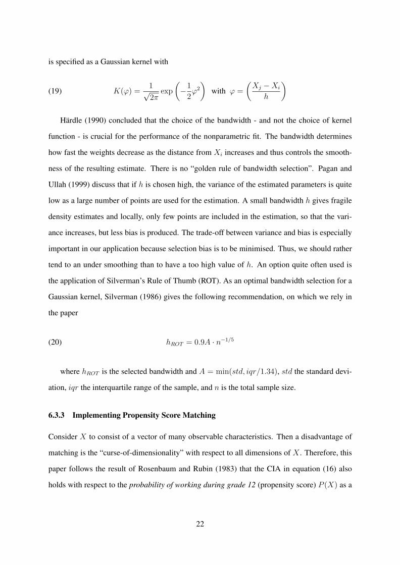
is specified as a Gaussian kernel with

(19) K(ϕ) =1√2π

exp

(−1

2ϕ2

)with ϕ =

(Xj −Xi

h

)

Härdle (1990) concluded that the choice of the bandwidth - and not the choice of kernel

function - is crucial for the performance of the nonparametric fit. The bandwidth determines

how fast the weights decrease as the distance from Xi increases and thus controls the smooth-

ness of the resulting estimate. There is no “golden rule of bandwidth selection”. Pagan and

Ullah (1999) discuss that if h is chosen high, the variance of the estimated parameters is quite

low as a large number of points are used for the estimation. A small bandwidth h gives fragile

density estimates and locally, only few points are included in the estimation, so that the vari-

ance increases, but less bias is produced. The trade-off between variance and bias is especially

important in our application because selection bias is to be minimised. Thus, we should rather

tend to an under smoothing than to have a too high value of h. An option quite often used is

the application of Silverman’s Rule of Thumb (ROT). As an optimal bandwidth selection for a

Gaussian kernel, Silverman (1986) gives the following recommendation, on which we rely in

the paper

(20) hROT = 0.9A · n−1/5

where hROT is the selected bandwidth and A = min(std, iqr/1.34), std the standard devi-

ation, iqr the interquartile range of the sample, and n is the total sample size.

6.3.3 Implementing Propensity Score Matching

Consider X to consist of a vector of many observable characteristics. Then a disadvantage of

matching is the “curse-of-dimensionality” with respect to all dimensions of X . Therefore, this

paper follows the result of Rosenbaum and Rubin (1983) that the CIA in equation (16) also

holds with respect to the probability of working during grade 12 (propensity score) P (X) as a

22

function of the observable characteristics X , i.e.

(21) E(Y C|D = 1, P (X)) = E(Y C|D = 0, P (X))

The propensity score allows a matching based on a one-dimensional probability. This

dimension-reduction diminishes the problem of finding adequate matches and the problem of

empty cells. However, propensity matching comes at the costs that the propensity score has to

be estimated itself9.

We estimate the propensity score as a parametric probit model following the standard ap-

proach used in the literature. The probit model of the propensity score estimates the probability

of working during grade 12 depending on observable covariates. In this model, the decision to

work during grade 12 depends on a number of observable characteristics that can be observed

for both groups.

These covariates should ideally include all important variables influencing the individual

decision to work or not during grade 12. Fortunately, we are able to access from the NELS

dataset an unusually rich set of observable characteristics which are likely to affect the em-

ployment status of twelfth graders. Table A (in appendix) provides descriptive statistics for the

covariates used in estimating the propensity score. The set of conditioning variables includes

standard individual, socio-economic, family background, school level and regional variables as

outlined in the literature (Lillydahl, 1990; Schoenhals et al, 1998; Tyler, 2003; Warren et al,

2000), as well as information on parental education expenditures, school problems including

absenteeism, conflicts, alcohol and drugs issues and finally students’ educational aspirations at

grade 8.

The results of the probit estimates, according to gender, for the propensity score associated

with working part-time during grade 1210 are reported in Table B (in appendix)11.

9Note that we use a bootstrap estimator, with 200 replications, for the standard errors of the estimated treatmenteffects in order to capture the estimation error in the propensity score.

10Additional probit results associated with other part-time work definitions are available upon request.11As detailed hereafter, for balancing reasons the estimations of the propensity score as well as the treatment

effects are stratified by gender.

23

Propensity score matching can only be successful concerning the conditioning on observ-

able characteristics if the estimated propensity scores of working students and non-working

students overlap sufficiently. We implement a common support requirement which led to the

discarding of three cases who were outside the common support region. Finally, after match-

ing, all observable characteristics should be balanced between working students and matched

comparison observations. We formally test on the significance of differences in observable

characteristics between the sample of working students and the matched control outcomes us-

ing t-tests. If the means of the two groups are statistically different from each other with

respect to the observable X , the t-test will indicate a failure of the matching. Results indicate

that propensity score matching was successful in balancing all observed covariates between

workers and matched controls. The only exception was for the variable gender. We therefore

decide to stratify the estimations by gender and report both male and female results.12

6.4 Controlling for unobservable individual characteristics

Most econometric literature makes use of the assumption that selection bias due to observ-

able characteristics and selection bias due to unobservable characteristics can be considered

separately (Heckman, Ichimura and Todd 1998). While matching estimators as well as other

solutions on selection bias due to observable characteristics cope with the influence of mea-

sured variables on the participation decision, selection bias due to unobservable characteristics

has to be dealt with differently.

To account for selection of unobservables, the empirical literature has pursued various

strategies, in particular difference-in-difference estimators (see Heckman, LaLonde and Smith,

1999). Such an approach requires panel data and builds on the assumption of time-invariant lin-

ear selection effects. This estimator extends simple before-after comparisons to determine the

treatment effect based on the presumption that the outcome variable can also change over time

due to reasons unrelated to the decision to work. Here, following Heckman, Ichimura, Smith

12We are happy to provide additional detail regarding the balancing properties on request.

24

and Todd (1998), we implement a conditional difference-in-differences estimator (CDiD). This

method combines a propensity score matching approach with DiD such that, at each period,

a counterfactual outcome for the working students at grade 12 if they were not working is

estimated semiparametrically. This technique presents both the advantage to relax the linear

assumption when controlling for observables relative to standard DiD and to control for unob-

servables exploiting the panel dimension of the data. Besides, Smith and Todd (2005) shows

that the difference-in-differences matching estimator performs the best among nonexperimental

matching based estimators.

The CDiD estimator is based on the assumption that treated and non-treated do not have

different time trend relative to their outcomes. In the case of different time trends, the estimated

effect of the treatment using a CDiD estimator will be biased due to unobservable differences

in group dynamics. Typically, a preprogramme test looking at the evolution of the outcomes

between grades 8 and 10 would already show a difference in the evolution of the scores of the

group of the treated and the untreated before the treatment (i.e. working part-time in grade 12)

even occurred. In order to allow differential time trends between treated and non-treated, we

also implement a matching approach combined with the difference-in-difference-in-differences

estimator (DiDiD)13. The latter approach is more robust as it allows to recover the average

treatment effect on the treated under more general conditions.

6.4.1 Conditional difference-in-differences in matched samples

For a treatment which takes place between two periods t and t′ with t > t′, the required identi-

fying assumption for the CDiD estimator can be represented by an assumption weaker than the

equations (15) and (21) (Heckman, Ichimura, Smith and Todd (1998)):

(22) E(Y Ct − Y Ct′ |D = 1, P (X)) = E(Y Ct − Y Ct′ |D = 0, P (X))

13The DiDiD approach is used on the same dataset by Sanz-de-Galdeano and Vuri (2007) in order to estimatethe effect of parental divorce on teenagers’ cognitive development. Relative to theirs, our estimation procedurerelaxes the linear functional form restrictions on observables thanks to the local linear matching approach.

25

Where Y Ct denotes the outcome of an untreated individual at period t.

In the following, we model the conditional difference-in-differences estimator within a regres-

sion framework. The implementation of this model requires matched samples of working stu-

dents14 and the estimated counterfactual non-working outcomes for this population for two or

more consecutive points in time. The NELS panel data provide information about test scores in

Mathematics and Reading for three grades (8, 10 and 12) and allow an appropriate implemen-

tation of this identification strategy. We adopt the following notations:

Yi,t is the outcome of interest (test score in Mathematics or Reading) for student i at period t

Di,s ∈ {0, 1} is a treatment dummy variable such that for all i and all s < 1992, Di,s = 0,

and Di,1992 = 1 if student i is working part-time during grade 12

The conditional difference-in-differences approach assumes that working students can be

observed for at least two periods (s ∈ {t′, t}, with t′ < t) and that there are matched outcomes

of students not working during grade 12 which are observed in these two periods. In the fol-

lowing, we rely on the formulation of the DiD framework proposed by Ashenfelter and Card

(1985). Let us suppose that Yi,t is generated by a components of variance process15:

(23) Yi,t = αi + µt + βDi,t + εi,t

where µt is a time-specific component, β represents the effect of part-time work during

grade 12, αi is an individual-specific component representing unobserved heterogeneity in

terms of attainment. Hereafter, we will denote by µ the time trend µ1992 − µ199016. Finally,

εi,t is an idiosyncratic shock with mean zero which is supposed to be serially uncorrelated.

In the first period t′ = 1990 we observe the following:

14Henceforth, individuals holding a part-time job during grade 12 will be simply referred to as “working”students.

15In the following, we will denote by Y Ti,t(resp.Y Cj,t) the outcome for the working student i at period t (resp.for the non-working student j at period t).

16Without loss of generality, we impose µ1990 = 0.

26

Yi,1990 = αi + εi,1990

Second, at the end of grade 12 in period t = 1992 we observe the base effect of grade 10

and additionally an effect of working in grade 12. For the second period, the model shows:

Yi,1992 = αi + µ+ βDi,1992 + εi,1992

A central assumption underlying this model is that both groups (working students and

matched non-working students) show the same general movement µ in their test scores over

time. This restriction will be relaxed later by relying on a difference-in-difference-in-differences

framework.

Under the DiD identifying assumption under which, in absence of part-time work during

grade 12, the average outcome for the treated would have experienced the same variation as

the average outcome for the untreated (conditional on the covariates)17, the average effect of

the treatment-on-the-treated β can be estimated consistently by the difference-in-differences in

means between working students and matched controls given as:

(24)1

N

∑i∈{D=1}

Y Ti,t − Y Ti,t′ −

∑j∈{D=0}

w(i, j)Y Cj,t −∑

j∈{D=0}

w(i, j)Y Cj,t′

6.4.2 Adjusting for possible differences in time trends

We also implement a difference-in-difference-in-differences estimator (DiDiD) with local lin-

ear matching which relies on a weaker identifying assumption. Unlike the CDiD estimator, it is

robust to potential differences in outcome trends between treated and untreated as long as these

trends are stable over time.

With a DiDiD approach, both outcomes can now follow group specific trends over time.

Therefore, the DiDiD model has less restricted assumptions about the difference between work-

17This is known as the parallel trend assumption.

27

ers and matched non-workers, allowing for differences in the development over time. The use

of a DiDiD model is justified in the context of education because the hypothesis of parallel time

trend may be too strong. In the education process, pupils go through an accumulation of knowl-

edge. Arguably, pupils differ not only in terms of level of success but also in terms of ability

to progress through time. For this reason, one may consider that the parallel trend assumption

must be relaxed to make sure that the results are not biased by the fact that pupils working part

time and pupil not working part time differ in unobservable characteristics correlated with their

ability to progress at school.

We implement this DiDiD estimator, controlling for observable characteristics semipara-

metrically by propensity score matching following the same approach as for the CDiD18. The

required identifying assumption is now weaker than the condition (22). Supposing the treat-

ment takes place between periods t and t′, with t > t′ > t′′, it is given by:

(25)

E((Y Ct−Y Ct′)−(Y Ct′−Y Ct′′)|D = 1, P (X)) = E((Y Ct−Y Ct′)−(Y Ct′−Y Ct′′)|D = 0, P (X))

The average effect of the treatment on the treated in the CDiDiD model will be identified as

the change after the treatment in the trend of progression for the outcome of the treated (relative

to the matched untreated).

The modeling of the DiDiD model requires three time periods, and we make use of infor-

mation for grade 8, 10 and 12 available from the NELS data. As before, we consider matched

samples between working and non-working students in three periods, so that

s ∈ {t = 1992, t′ = 1990, t′′ = 1988}

Let us suppose that Yi,t, the test score for individual i at period t, is generated by an aug-

mented components of variance process which relaxes the assumption of identical time-specific

component by allowing for different time trends between the groups of treated and untreated

18In the following we refer to this as the CDiDiD estimator, exploiting the analogy with the CDiD approach.

28

individuals:

Yi,t = αi + µi,t + βDi,t + εi,t

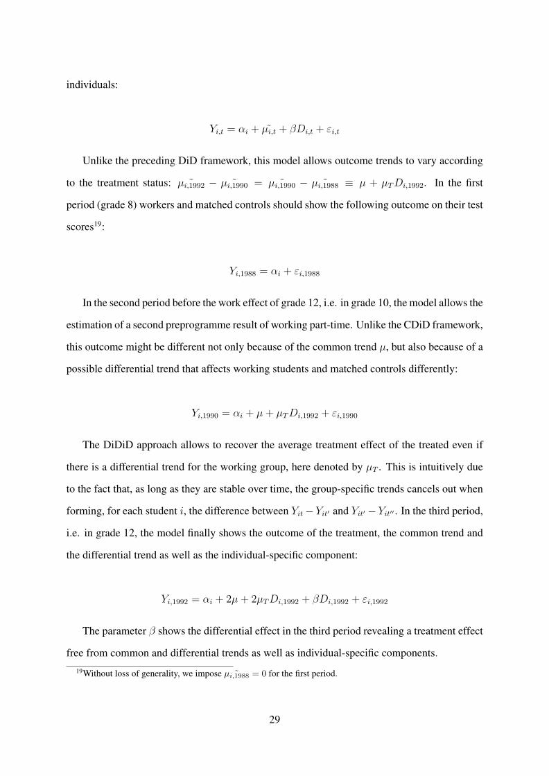
Unlike the preceding DiD framework, this model allows outcome trends to vary according

to the treatment status: ˜µi,1992 − ˜µi,1990 = ˜µi,1990 − ˜µi,1988 ≡ µ + µTDi,1992. In the first

period (grade 8) workers and matched controls should show the following outcome on their test

scores19:

Yi,1988 = αi + εi,1988

In the second period before the work effect of grade 12, i.e. in grade 10, the model allows the

estimation of a second preprogramme result of working part-time. Unlike the CDiD framework,

this outcome might be different not only because of the common trend µ, but also because of a

possible differential trend that affects working students and matched controls differently:

Yi,1990 = αi + µ+ µTDi,1992 + εi,1990

The DiDiD approach allows to recover the average treatment effect of the treated even if

there is a differential trend for the working group, here denoted by µT . This is intuitively due

to the fact that, as long as they are stable over time, the group-specific trends cancels out when

forming, for each student i, the difference between Yit−Yit′ and Yit′ −Yit′′ . In the third period,

i.e. in grade 12, the model finally shows the outcome of the treatment, the common trend and

the differential trend as well as the individual-specific component:

Yi,1992 = αi + 2µ+ 2µTDi,1992 + βDi,1992 + εi,1992

The parameter β shows the differential effect in the third period revealing a treatment effect

free from common and differential trends as well as individual-specific components.

19Without loss of generality, we impose ˜µi,1988 = 0 for the first period.

29

Finally, under the identifying assumption (25) stated above, the average effect of the treatment-

on-the-treated β can be estimated consistently by the difference-in-difference-in-differences in

means between working students and matched controls. The expression of the estimator can be

straightforwardly obtained by transposing the preceding expression of the CDiD estimator to a

DiDiD framework.

7 Results

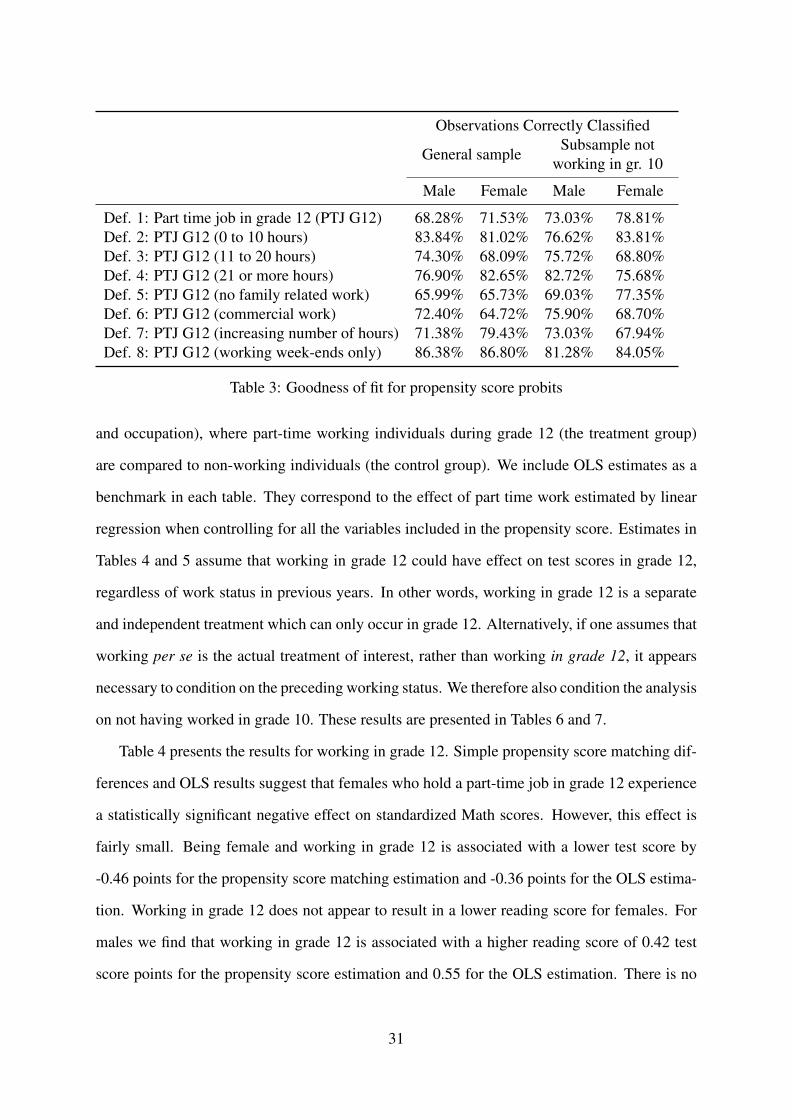
The propensity score matching proved to be successful for the different definitions of the part

time job treatment variable that we studied. Table 3 shows that the goodness of fit of the probit

is rather good, on average they predict correctly the treatment status in 75% of the case.

In addition, our propensity scores show a large common support which is important in order

for the propensity score approach to be valid (Smith and Todd, 2005). To define the common

support region we trimmed observations with no overlap between the two propensity scores.

Given the very good overlap this led to only discarding three observations. As Bryson et al.

(2002) indicate, the common support restriction is not a problem when only few observations

have to be discarded. This is illustrated below in Figure 1, which reports the kernel density

estimates of the propensity scores for working and non-working students, according to gender.

Figure 1: Common support of the propensity scores

Tables 4 to 7 present the results for different types of part-time work (measured by intensity

30

Observations Correctly Classified

General sampleSubsample not

working in gr. 10

Male Female Male Female

Def. 1: Part time job in grade 12 (PTJ G12) 68.28% 71.53% 73.03% 78.81%Def. 2: PTJ G12 (0 to 10 hours) 83.84% 81.02% 76.62% 83.81%Def. 3: PTJ G12 (11 to 20 hours) 74.30% 68.09% 75.72% 68.80%Def. 4: PTJ G12 (21 or more hours) 76.90% 82.65% 82.72% 75.68%Def. 5: PTJ G12 (no family related work) 65.99% 65.73% 69.03% 77.35%Def. 6: PTJ G12 (commercial work) 72.40% 64.72% 75.90% 68.70%Def. 7: PTJ G12 (increasing number of hours) 71.38% 79.43% 73.03% 67.94%Def. 8: PTJ G12 (working week-ends only) 86.38% 86.80% 81.28% 84.05%

Table 3: Goodness of fit for propensity score probits

and occupation), where part-time working individuals during grade 12 (the treatment group)

are compared to non-working individuals (the control group). We include OLS estimates as a

benchmark in each table. They correspond to the effect of part time work estimated by linear

regression when controlling for all the variables included in the propensity score. Estimates in

Tables 4 and 5 assume that working in grade 12 could have effect on test scores in grade 12,

regardless of work status in previous years. In other words, working in grade 12 is a separate

and independent treatment which can only occur in grade 12. Alternatively, if one assumes that

working per se is the actual treatment of interest, rather than working in grade 12, it appears

necessary to condition on the preceding working status. We therefore also condition the analysis

on not having worked in grade 10. These results are presented in Tables 6 and 7.

Table 4 presents the results for working in grade 12. Simple propensity score matching dif-

ferences and OLS results suggest that females who hold a part-time job in grade 12 experience

a statistically significant negative effect on standardized Math scores. However, this effect is

fairly small. Being female and working in grade 12 is associated with a lower test score by

-0.46 points for the propensity score matching estimation and -0.36 points for the OLS estima-

tion. Working in grade 12 does not appear to result in a lower reading score for females. For

males we find that working in grade 12 is associated with a higher reading score of 0.42 test

score points for the propensity score estimation and 0.55 for the OLS estimation. There is no

31

significant effect on math score for males.

Such results are interesting as they suggest differential effects of working during school

not just by gender, but also by subject. However, examining the conditional difference-in-

differences estimates we find that all coefficients now become statistically insignificant. Sim-

ilarly, the CDiDiD model gives non significant results. This suggest that once we control for

unobservable time invariant characteristics, all effects of working part-time disappear. Hence

previous estimates, whilst controlling for observable characteristics, failed to take into account

unobserved heterogeneity among individuals and as such, prescribed a spurious treatment ef-

fect to working. Once controlled for, any effect of working in grade 12 disappears, suggesting

that working in grade 12 has no significant causal impact on educational attainment. Whilst we

offer different definitions of working in grade 12, this is a story which repeats itself throughout

the results and can be taken as the main result from this analysis.

Continuing to examine Table 4 for differences in the amount of hours worked per week in

grade 12, we find that OLS estimates yield small positive effects from working 0 to 10 hours

per week for both males and females (a result commonly found in the literature). However,

propensity score matching estimates increase the standard error (and for males reduce the point

estimates) of these estimates which reduces them to insignificance. Working 10 to 20 hours

per week has no effect on females for any estimation procedure20 whilst we estimate a posi-

tive association with male reading scores in the OLS and propensity score matching analysis

(estimates of 0.60 and 0.67 respectively). Such results could suggest that men experience the

positive benefits of working during school at a higher level of hours worked. However, work-

ing many hours per week (21 hours or more) has a significant negative impact on female maths

and reading scores for both OLS and propensity score matching estimates (with estimates be-

tween -0.68 and -0.88). There is also some negative effect on male Math scores for the OLS

and propensity score matching estimates (with estimates between -0.50 and -0.68) whilst the

previous positive effect on reading test scores disappears into statistical insignificance.

Using OLS and propensity score matching only, the above results would highlight a story

20This may be due to the inflection point occurring somewhere in this region.

32

which appears to be similar to general findings in much of the previous literature – namely the

inverted ‘u-shaped’ return, in terms of educational attainment, to working during school (albeit

interesting differences by gender and subject type exist). However, all conditional DiD and Di-

DiD estimates reduce the point estimates and yield statistical insignificance of the results. This

suggests that the previous pattern found in the literature on the effect of high school employ-

ment on test scores is most likely to be due to selection on unobservables21 related to part-time

work decisions.

Is is noteworthy that, relatively to the previous work of Tyler (2003) on the same dataset,

the non significance of our results is not only driven by higher standard errors of our estimates.

Indeed, in his article Tyler found a negative effect of around 0.20 per hour of part time work

on Maths and Reading scores in grade 12. In comparison our point estimates are suggesting a

much lower hourly effect: the estimated effect of working more than 21 hours is for instance

always below 1, which is consistent with an hourly effect below 0.05.

Turning to Table 5, where we examine different forms of occupation and weekend work,

we find once again that none of the conditional DiD and DiDiD estimates are statistically sig-

nificant. Whilst there is some suggestion in the OLS and propensity score matching estimates

that working in the “mainstream” work categories (grocery clerk, fast food and salespersons) is

slightly detrimental for women, with respect to Reading test scores, and slightly beneficial for

males, difference-in-differences estimates suggest that such significant results can be explained

away by considering previous test score movements.

Examining Table 6 and 7, where we condition on not having worked part-time in grade 10,

we find that, generally speaking, most of the estimates are very similar to the previous results

where we do not condition on previous work experience. Matching simple differences and OLS

suggest that females now experience a higher detrimental effect on reading and math scores

from working more than 21 hours (-1.61 and -1.05 respectively for the matching estimates).

However, like the previous estimates, no significance is detected in the conditional DiD as well

21Besides, given that both cDiD and cDiDiD yield insignificant estimates, our results also suggest that thesignificant effects which are found when controlling for selection on observables are due to selection on time-invariant unobservable characteristics.

33

Part-time work effect, job definition 1 Part-time work effect, job definition 3

Anyone who has a part-time job in grade 12 Anyone who has a part-time job in grade 12and works 11 to 20 hours per week

Evaluation outcomes Evaluation outcomes

Females Males Females MalesCoef. S.E. Sign. Coef. S.E. Sign. Coef. S.E. Sign. Coef. S.E. Sign.

Math, OLS -0.36∗ 0.15 0.02 0.05 0.17 0.75 Math, OLS -0.14 0.14 0.33 0.34† 0.18 0.06Read, OLS -0.14 0.17 0.55 0.55∗∗ 0.21 0.01 Read, OLS 0.14 0.17 0.41 0.60∗∗ 0.222 0.01Math, PMatch -0.46∗∗ 0.16 0.00 -0.13 0.17 0.46 Math, PMatch -0.34 0.24 0.15 0.16 0.27 0.55Read, PMatch -0.19 0.15 0.21 0.42∗∗ 0.17 0.01 Read, PMatch -0.09 0.22 0.71 0.67∗ 0.28 0.02Math, DID -0.29 0.22 0.20 -0.13 0.24 0.60 Math, DID -0.22 0.33 0.50 0.06 0.39 0.88Read, DID -0.29 0.22 0.19 0.22 0.24 0.35 Read, DID -0.02 0.32 0.95 0.42 0.40 0.28Math, DIDID -0.35 0.40 0.38 -0.17 0.43 0.68 Math, DIDID -0.29 0.59 0.62 0.02 0.69 0.98Read, DIDID -0.49 0.39 0.21 -0.08 0.42 0.85 Read, DIDID 0.05 0.57 0.93 0.10 0.69 0.89

Part-time work effect, job definition 2 Part-time work effect, job definition 4Anyone who has a part-time job in grade 12

and works 0 to 10 hours per weekAnyone who has a part-time job in grade 12

and works 21 or more hours per weekEvaluation outcomes Evaluation outcomes

Females Males Females MalesCoef. S.E. Sign. Coef. S.E. Sign. Coef. S.E. Sign. Coef. S.E. Sign.

Math, OLS 0.34∗ 0.17 0.04 0.47∗ 0.21 0.02 Math, OLS -0.68∗∗ 0.18 0.00 -0.68∗∗ 0.19 0.00Read, OLS 0.37† 0.20 0.06 0.36 0.26 0.17 Read, OLS -0.82∗∗ 0.21 0.04 -0.24 0.23 0.30Math, PMatch 0.26 0.38 0.49 0.01 0.32 0.97 Math, PMatch -0.70∗ 0.31 0.02 -0.50† 0.29 0.09Read, PMatch 0.44 0.38 0.24 0.05 0.31 0.87 Read, PMatch -0.88∗∗ 0.31 0.00 0.32 0.29 0.28Math, DID -0.08 0.53 0.88 -0.01 0.46 0.99 Math, DID -0.35 0.44 0.42 -0.35 0.42 0.40Read, DID -0.11 0.53 0.84 -0.21 0.44 0.63 Read, DID -0.97 0.65 0.14 0.27 0.41 0.52Math, DIDID -0.39 0.95 0.68 0.08 0.82 0.93 Math, DIDID 0.06 0.77 0.94 -0.25 0.73 0.73Read, DIDID -0.67 0.93 0.47 -0.47 0.79 0.56 Read, DIDID -0.96 0.77 0.21 0.01 0.72 0.99

Significant at: † 10%, ∗ 5%, ∗∗ 1%.

Table 4: Estimation of the effect of part time work unconditional on working in grade 10:decomposition by hours

as DiDiD estimates, suggesting again that once controlling for selection on observables and

unobservables, any effect of working part-time during grade 12 on standardized test scores

disappears.

34

Part-time work effect, job definition 5 Part-time work effect, job definition 7Anyone who has a part-time job in grade 12

but does not work as a babysitter, lawn or household workerOnly those who have a part-time job in grade 12

and increased their work hours from grade 10Evaluation outcomes Evaluation outcomes

Females Males Females MalesCoef. S.E. Sign. Coef. S.E. Sign. Coef. S.E. Sign. Coef. S.E. Sign.

Math, OLS -0.35∗ 0.14 0.01 0.11 0.16 0.52 Math, OLS -0.07 0.16 0.69 0.05 0.17 0.78Read, OLS -0.16 0.16 0.33 0.60∗∗ 0.20 0.00 Read, OLS -0.23 0.20 0.22 -0.33 0.22 0.13Math, PMatch -0.46∗∗ 0.17 0.01 -0.11 0.17 0.53 Math, PMatch -0.69∗ 0.33 0.03 0.06 0.29 0.83Read, PMatch -0.31∗ 0.16 0.05 0.43∗∗ 0.17 0.01 Read, PMatch -0.23 0.31 0.46 -0.10 0.30 0.74Math, DID -0.19 0.24 0.42 -0.10 0.25 0.68 Math, DID -0.39 0.46 0.40 -0.31 0.42 0.46Read, DID -0.25 0.23 0.28 0.22 0.25 0.38 Read, DID -0.09 0.44 0.84 -0.50 0.43 0.25Math, DIDID -0.14 0.42 0.74 -0.15 0.44 0.74 Math, DIDID -0.22 0.82 0.79 -0.74 0.74 0.32Read, DIDID -0.32 0.41 0.44 -0.09 0.43 0.84 Read, DIDID -0.15 0.79 0.85 -1.12 0.74 0.13

Part-time work effect, job definition 6 Part-time work effect, job definition 8Only those who have a part-time job in grade 12

and are salespersons, fast food workers or grocery clerks Only those who work weekends only in grade 12

Evaluation outcomes Evaluation outcomes

Females Males Females MalesCoef. S.E. Sign. Coef. S.E. Sign. Coef. S.E. Sign. Coef. S.E. Sign.

Math, OLS 0.52 0.14 0.71 0.47∗∗ 0.17 0.01 Math, OLS 0.29 0.19 0.13 0.34 0.22 0.13Read, OLS -0.05 0.17 0.78 0.92∗∗ 0.22 0.00 Read, OLS 0.38† 0.23 0.10 0.17 0.28 0.54Math, PMatch -0.33 0.22 0.13 0.17 0.27 0.52 Math, PMatch -0.10 0.38 0.79 0.15 0.41 0.71Read, PMatch -0.36† 0.21 0.09 0.81∗∗ 0.26 0.00 Read, PMatch 0.15 0.36 0.68 0.43 0.41 0.30Math, DID -0.21 0.31 0.50 -0.05 0.38 0.89 Math, DID 0.12 0.54 0.82 -0.07 0.57 0.91Read, DID -0.31 0.30 0.30 0.10 0.38 0.80 Read, DID -0.24 0.52 0.65 -0.27 0.58 0.65Math, DIDID -0.25 0.55 0.65 -0.33 0.67 0.62 Math, DIDID 0.30 0.98 0.76 -0.24 1.02 0.81Read, DIDID -0.36 0.54 0.51 -0.71 0.66 0.28 Read, DIDID -0.69 0.93 0.46 -1.02 1.01 0.32

Significant at: † 10%, ∗ 5%, ∗∗ 1%.

Table 5: Estimation of the effect of part time work unconditional on working in grade 10:decomposition by type of work

Part-time work effect, job definition 1 Part-time work effect, job definition 3

Anyone who has a part-time job in grade 12 Anyone who has a part-time job in grade 12and works 11 to 20 hours per week

Evaluation outcomes Evaluation outcomesFemales Males Females Males

Coef. S.E. Sign. Coef. S.E. Sign. Coef. S.E. Sign. Coef. S.E. Sign.Math, OLS -0.47∗ 0.20 0.02 -0.09 0.26 0.72 Math, OLS -0.32 0.21 0.14 -0.26 0.32 0.42Read, OLS -0.17 0.24 0.47 0.31 0.32 0.34 Read, OLS -0.07 0.26 0.78 0.38 0.40 0.34Math, PMatch -0.54∗ 0.23 0.02 -0.40 0.28 0.15 Math, PMatch -0.44 0.35 0.21 -0.30 0.47 0.53Read, PMatch -0.31 0.22 0.16 -0.28 0.28 0.32 Read, PMatch -0.11 0.34 0.75 -0.04 0.48 0.94Math, DID -0.33 0.32 0.32 -0.19 0.40 0.63 Math, DID -0.49 0.49 0.32 -0.13 0.67 0.84Read, DID -0.33 0.32 0.30 -0.06 0.40 0.88 Read, DID -0.16 0.48 0.74 -0.18 0.68 0.80Math, DIDID -0.17 0.57 0.77 -0.08 0.69 0.90 Math, DIDID -0.51 0.87 0.56 -0.05 1.16 0.97Read, DIDID -0.37 0.56 0.51 -0.10 0.69 0.88 Read, DIDID -0.07 0.85 0.94 -0.54 1.18 0.65

Part-time work effect, job definition 2 Part-time work effect job definition 4Anyone who has a part-time job in grade 12

and works 0 to 10 hours per weekAnyone who has a part-time job in grade 12

and works 21 or more hours per weekEvaluation outcomes Evaluation outcomes

Females Males Females MalesCoef. S.E. Sign. Coef. S.E. Sign. Coef. S.E. Sign. Coef. S.E. Sign.

Math, OLS 0.38 0.25 0.12 0.40 0.36 0.27 Math, OLS -0.85∗∗ 0.27 0.00 -0.21 0.33 0.53Read, OLS 0.27 0.30 0.04 0.04 0.46 0.94 Read, OLS -0.54 0.33 0.11 0.06 0.42 0.88Math, PMatch -0.23 0.45 0.62 -0.03 0.58 0.96 Math, PMatch -1.61∗∗ 0.45 0.00 -0.38 0.50 0.44Read, PMatch -0.19 0.44 0.67 -0.30 0.59 0.62 Read, PMatch -1.05∗ 0.45 0.02 0.20 0.50 0.69Math, DID -0.13 0.65 0.85 -0.25 0.83 0.77 Math, DID -0.54 0.64 0.40 -0.28 0.71 0.70Read, DID -0.10 0.63 0.88 -0.61 0.84 0.47 Read, DID -0.96 0.65 0.14 0.29 0.70 0.68Math, DIDID -0.09 1.16 0.94 -0.42 1.48 0.77 Math, DIDID -0.03 1.11 0.98 -0.23 1.22 0.85Read, DIDID -0.09 1.13 0.94 -0.98 1.47 0.50 Read, DIDID -1.34 1.13 0.24 0.21 1.20 0.86

Significant at: † 10%, ∗ 5%, ∗∗ 1%.

Table 6: Estimation of the effect of part time work conditional on not working in grade 10:decomposition by hours

35

Part-time work effect, job definition 5 Part-time work effect, job definition 7Anyone who has a part-time job in grade 12

but does not work as a babysitter, lawn or household workerOnly those who have a part-time job in grade 12

and increased their work hours from grade 10Evaluation outcomes Evaluation outcomes

Females Males Females MalesCoef. S.E. Sign. Coef. S.E. Sign. Coef. S.E. Sign. Coef. S.E. Sign.

Math, OLS -0.45∗ 0.19 0.02 -0.04 0.26 0.88 Math, OLS -0.47 0.20 0.02 -0.09 0.26 0.72Read, OLS -0.17 0.24 0.47 0.24 0.33 0.46 Read, OLS -0.17 0.24 0.47 0.31 0.32 0.34Math, PMatch -0.55∗ 0.24 0.02 -0.42 0.29 0.14 Math, PMatch -0.54∗ 0.23 0.02 -0.40 0.28 0.15Read, PMatch -0.31 0.23 0.19 -0.29 0.29 0.32 Read, PMatch -0.31 0.22 0.02 -0.28 0.40 0.63Math, DID -0.36 0.34 0.29 -0.17 0.41 0.67 Math, DID -0.33 0.32 0.32 -0.19 0.40 0.63Read, DID 0.10 0.35 0.77 -0.05 0.41 0.89 Read, DID -0.33 0.32 0.30 -0.06. 0.40 0.88Math, DIDID -0.21 0.60 0.72 -0.05 0.71 0.95 Math, DIDID -0.17 0.57 0.77 -0.08 0.69 0.90Read, DIDID -0.48 0.59 0.41 -0.08 0.70 0.90 Read, DIDID -0.37 0.56 0.51 -0.10 0.69 0.88

Part-time work effect, job definition 6 Part-time work effect, job definition 8Only those who have a part-time job in grade 12

and are salespersons, fast food workers or grocery clerks Only those who work weekends only in grade 12

Evaluation outcomes Evaluation outcomesFemales Males Females Males

Coef. S.E. Sign. Coef. S.E. Sign. Coef. S.E. Sign. Coef. S.E. Sign.Math, OLS -0.34 0.21 0.10 0.36 0.30 0.24 Math, OLS 0.25 0.30 0.40 0.14 0.43 0.74Read, OLS 0.14 0.25 0.57 0.57 0.38 0.13 Read, OLS 0.70∗ 0.36 0.05 0.71 0.53 0.18Math, PMatch -0.28 0.32 0.38 -0.15 0.44 0.73 Math, PMatch -0.22 0.57 0.70 -0.66 0.69 0.33Read, PMatch 0.17 0.31 0.58 -0.03 0.45 0.94 Read, PMatch 0.27 0.52 0.61 0.07 0.70 0.92Math, DID -0.57 0.45 0.21 -0.16 0.63 0.80 Math, DID 0.02 0.81 0.98 -0.53 0.96 0.58Read, DID 0.06 0.46 0.90 -0.26 0.64 0.69 Read, DID 0.18 0.82 0.83 -0.86 0.99 0.38Math, DIDID -0.46 0.80 0.57 -0.31 1.09 0.78 Math, DIDID 0.26 1.45 0.86 -0.77 1.70 0.65Read, DIDID -0.45 0.78 0.57 -0.88 1.11 0.43 Read, DIDID -0.14 1.37 0.92 -1.98 1.72 0.25

Significant at: † 10%, ∗ 5%, ∗∗ 1%.By definition results for job definition 7 are the same as for job definition 1

Table 7: Estimation of the effect of part time work conditional on not working in grade 10:decomposition by type of work

8 Conclusion

In this paper we contribute to the literature regarding the effect of working while studying by

employing a semiparametric propensity score matching approach combined with difference-

in-differences in order to address in a flexible way selection on observables as well as unob-

servables associated with part-time work decisions during grade 12. Unlike most of previous

attempts to control for the endogeneity of part-time work status our approach does not consist

in finding an instrument, whose validity is often questionable, for part-time work decisions.

Our identification strategy takes advantage of the longitudinal nature of the NELS:88 as well

as its unusual richness in terms of variables related to part-time work decisions and educational

outcomes, which is, as it is shown by Smith and Todd (2005), central for a matching-based

estimator to perform well. Results indicate that, once selection is controlled for, we find no

significant evidence of working during grade 12 affecting mathematics or reading test scores.

In line with most of the recent papers estimating the impact of part-time work on educa-

tional attainment, our analysis suggests that OLS results are biased because of a selection on

unobservables. While some positive effect of a small amount of part time work and a detrimen-

36

tal effect of a large amount of part time work can be found when controlling for differences

in observable characteristic, no significant effect remains when we also control for differences

in unobservable characteristics using conditional difference-in-differences and difference-in-

difference-in-differences. This suggests that the significant associations initially estimated be-

tween part-time work during grade 12 and standardized test scores are actually due to selection

on unobservables. Typically, pupils choosing to take on a small amount of part time work

tend to have unobserved characteristics linked with better academic achievement while pupils

choosing to take on a large amount of part time work tend to have unobserved characteristics

linked with lower academic achievement22.

In conclusion, we find that the causal effect on educational attainment of working during

grade 12 in high school is negligibly small. Furthermore we find no evidence of different job

types significantly influencing reading and mathematics score. The fact that, once unobserv-

able characteristics are controlled for, we obtain different results compared to simple matching

estimates indicates that the negative association which is sometimes found between educational

attainment and part-time work is unlikely to transmit itself through working per se, but through

unobservable characteristics. Our results suggest a negligible academic cost, in terms of test

scores, to part-time working during grade 12. From a policy point of view one could thus

argue that more stringent child labour laws are unlikely to be conductive in achieving higher

attainment scores and that, as regards to educational achievement, working during high school

should be neither encouraged nor discouraged.

References

Abadie, A. and Imbens, G. (2006), “On the failure of the Bootstrap for Matching Estimators”,

NBER Working Paper No. T0325.

Ashenfelter, O. and Card, D. (1985) “Using the Longitudinal Structure of Earnings to Esti-

mate the Effect of Training Programs”, The Review of Economics and Statistics, Vol. 67, No.

22Among others, this may stem from a lower ability or motivation for schooling.

37

4, pp. 648-660.

Dorsett, R. (2005) “Unemployed Couples: The labour market effects of making both parties

search for work”, Journal of the Royal Statistical Society: Series A, Vol. 168, No. 2, pp.365-

385.

Bergemann, A., Fitzenberger, B. and Speckesser, S. (2005), “Evaluating the Dynamic Em-

ployment Effects of Training Programs in East Germany Using Conditional Difference-in-

Differences”, IZA Discussion Paper 1648, Bonn: Institute for the Study of Labor (IZA).

Bryson, A., Dorsett, R. and Purdon, S. (2002) The use of propensity score matching in the

evaluation of labour market policies. Working Paper No. 4, Department for Work and Pensions.

Cheng, Y. (1995) “Staying on in Full-time Education after 16: Do schools make a differ-

ence?” Department for Education and Employment Research Studies, Youth Cohort Report

37.

Coleman, J.S. (1961) The Adolescent Society, Glencoe, IL: Free Press.

D’Amico, R. (1984) “Does Employment during High School impair Academic Progress?”,

Sociology of Education, Vol. 57, pp. 152-164.

Dustmann, C. and van Soest, A. (2007) “Part-time Work, School Success and School Leav-

ing”, Empirical Economics, Vol. 32, pp.277-299.

Eckstein, Z. and Wolpin, K.I. (1999) “Why Youth Drop out of High School: The Impact of

Preferences, Opportunities and Abilities”, Econometrica, Vol. 67, No. 2, pp. 1295-1339.

Ehrenberg, R.G and Sherman, D.R. (1987) “Employment While in College, Academic

Achievement, and Post-College Outcomes: A Summary of Results”, The Journal Of Human

Resources, Vol. 22, No. 1, pp. 1-23.

Fan, J. (1993) “Local Linear Regression Smoothers and Their Minimax Efficiencies”, The

Annals of Statistics, Vol. 21, No. 1, pp. 196-216.

Green, G. and Jacques, S. (1987) “The Effect of Part-Time Employment on Academic

Achievement”, Journal of Educational Research, Vol. 80, pp. 325-329.

Greenberger, E. and Steinberg, L.D., Vaux, A., and McAuliffe, S. (1980) “Adolescents Who

Work: Effects of Part-Time Employment on Family and Peer Relations”, Journal of Youth and

38

Adolescence, Vol. 9, pp. 189-202.

Greenberger, E. and Steinberg, L.D. (1980) “Part-time employment of in-school youths:

A preliminary assessment of costs and benefits” In A review of Youth Problems, Programs

and Policies, compiled by I.S. Vice President”s Task Force on Youth Employment, pp. 1-15.

Washington, DC: U.S. Department of Labor, Employment and training Administration.

Härdle,W. (1990), Applied nonparametric regression, volume 19 of Econometric Society

Monographs. Cambridge University Press.

Heckman, J., Ichimura, H., Smith, J. and Todd, P. (1998), “Characterizing Selection Bias

Using Experimental Data”, Econometrica, Vol. 66, pp. 1017-1098.

Heckman, J., Ichimura, H. and Todd, P. (1998), “Matching as an Econometric Evaluation

Estimator”, Review of Economic Studies, Vol. 65, pp. 261-294.

Heckman, J.J. and V.J. Hotz (1989), SChoosing among Alternative Nonexperimental Meth-

ods for Estimating the Impact of Social Programs: The Case of Manpower TrainingT, Journal

of the American Statistical Association 84, 862-874.

Heckman, J., LaLonde, R.J. and Smith, J.A. (1999) “The Economics and Econometrics of

Active Labor Market Programs”, in Ashenfelter, O. and D. Card (ed.), Handbook of Labor

Economics, Amsterdam: North Holland.

Holland, A. and Andre, T. (1987) “Participation in Extracurricular Activities in Secondary

School: What is known, What Needs to Be Known?”, Review of Educational Research, Vol.

57, pp. 437-466.

Lewin-Epstein, N. (1981) Youth Employment during High School: An analysis of High

School and Beyond. National Center for Educational Statistics.

Lillydahl, J.H. (1990) “Academic Achievement and part-Time Employment of High-School

students”, Journal of Economic Education, Vol. 21, pp. 307-316.

Marsh, H.W. (1991) “Employment during High School: Character building or a subversion

of academic goals?”, Sociology of Education, Vol. 64, pp. 172-189.

Meyer, R.H. and Wise, D.A. (1982) “High School Preparation and Early Labor Force Ex-

perience” In Youth Labor Market Problem: Its Nature, Causes and Consequences, edited by

39

Freeman, R.G. and Wise, D.A., pp. 277-341, Chicago: University of Chigaco Press.

Michael, R.T., and Tuma, N.B. (1984) “Youth Employment: Does life begin at 16?”, Jour-

nal of Labor Economics, Vol. 2, No. 4, pp. 464-476.

Montmarquette, C., Viennot-Briot, N., and Dagenais, M. (2007) “Dropout, School Perfor-

mance, and Working while in School”, The Review of Economics and Statistics, Vol.89, No.4,

pp. 752-760.

Mortimer, J.T., Finch, M., Shanahan, M., and Ryu, S. (1992) “Work Experience, Mental

Health, and Behavioural Adjustment in Adolescence”, Journal of Research on Adolescence,

Vol. 2, No.1, pp. 25-57.

Oettinger, S.G. (1999) “Does High School Employment Affect High School Academic Per-

formance?” Industrial and Labor Relations Review, Vol. 53, No. 1, pp. 136-151.

Pagan, A. and Ullah, A. (1999), Nonparametric Econometrics, Cambridge University Press.

Rothstein, D.S. (2007) “High School Employment and Youths Academic Achievement”,

The Journal of Human Resources, Vol. 42, pp. 194-213.

Rosenbaum, P.R. and Rubin, D.B. (1983), “The central role of the propensity score in ob-

servational studies for causal effects”, Biometrika, Vol. 70, pp. 41-55.

Roy, A. (1951), “Some Thoughts on the Distribution of Earnings”, Oxford Economic Pa-

pers, Vol. 3, pp. 135-146.

Rubin, D. (1974), “Estimating Causal Effects of Treatments in Randomized and Nonran-

domized Studies”, Journal of Educational Psychology, 66, 688-701.

Ruhm, C.J. (1995) “The Extent and Consequences of High School Employment” Journal

of Labor Research, Vol. 16, pp. 291-303.

Ruhm, C.J. (1997) “Is High School Employment Consumption or Investment?”, Journal of

Labor Economics, Vol. 15, No. 4, pp. 725-776.

Sanz-de-Galdeano, A. and Vuri, D. (2007) “Parental Divorce and Students’ Performance:

Evidence from Longitudinal Data”, Oxford Bulletin of Economics and Statistics, Vol. 69, No.

3, pp. 321-338.

Schill, W.J., McCartin, R., & Meyer, K. (1985). “Youth Employment: Its Relationship to

40

Academic and Family Variables”, Journal of Vocational Behaviour, Vol 26, pp.155-163.

Schoenhals, M., Tienda, M. and Schneider, B. (1998) “The Educational and Personal Con-

sequences of Adolescent Employment”, Social Forces, Vol. 77, pp. 723-762.

Silverman, B.W. (1986), Density estimation for statistics and data analysis, Chapman and

Hall, London, England.

Singh. K. (1998) “Part-time Employment in High School and its Effect on Academic

Achievement”, Journal of Educational Research, Vol. 91, pp. 131-139.

Smith, J. and Todd, P. (2005) “Does matching overcome LaLonde’s critique of nonexperi-

mental estimators?”, Journal of Econometrics, Vol. 125, pp. 305-353.

Steel, L. (1991) “Early Work Experience Among White and Non-White Youth”, Youth and

Society, Vol. 22, No. 4, pp. 419-447.

Steinberg, L. and Greenberger, E. (1980) “The Part-Time Employment of High School

Students: A Research Agenda”, Children and Youth Services Review, Vol. 2, pp. 161-185.

Steinberg, L. D., Greenberger, E., Garduque, L., & McAuliffe, S. (1982) “High School

Students in the Labor Force: Some Costs and Benefits to Schooling and Learning”, Educational

Evaluation and Policy Analysis, Vol. 4, No. 3, pp. 363-372.

Stinebrickner, R. and Stinebrickner, T.R. (2003) “Working during School and Academic

Performance”, Journal of Labor Economics, Vol 21. No. 2, pp. 473-491.

Turner, M.D. (1994) “The Effects of Part-Time Work on High School Students’ Academic

Achievement”, unpublished paper, College Park: University of Maryland.

Tyler, J.H. (2003) “Using State Child Labor Laws to Identify the Effect of School-Year

Work on High School Achievement”, Journal of Labor Economics, Vol 21. No. 2. pp. 381-

408.

Warren, J.R., LePore, P.C., and Mare, R.D. (2000) “Employment During High School:

Consequences for Students’ Grades in Academic Courses”, American Educational Research

Journal, Vol. 37, pp. 943-969.

Warren, J.R. (2002) “Reconsidering the Relationship between Student Employment and

Academic Outcomes: A New Theory and Better Data”, Youth and Society, Vol. 33, No. 3, pp.

41

366-393.

Worley, L.P. (1995) “Working adolescents: Implication for counsellors” The School Coun-

selor, Vol. 42, pp 218-223.

9 Appendix

Table A: Descriptive statistics of the variables included in the probits

Working Not Working

Frequency Percent Frequency Percent

GenderMales 3,079 46.73 1,649 50.00Females 3,510 53.27 1,649 50.00Parental EducationNone 369 5.60 247 7.49High school 1,089 16.53 511 15.49Graduate high school (<4 yrs) 2,584 39.22 1,053 31.93College graduate 1,044 15.84 541 16.40MA./MSc 664 10.08 378 11.46PhD/M.D. 291 4.42 359 10.89Missing 548 8.32 209 6.34

Parental EmploymentFather is unemployed 643 9.76 423 12.83Father is employed 5,946 90.24 2,875 87.17Mother is unemployed 634 9.62 371 11.25Mother is employed 5,955 90.38 2,927 88.75Mother’s OccupationOffice Worker 1,557 23.63 605 18.34Tradeperson 120 1.82 65 1.97Farmer 20 0.30 17 0.52F-T Homemaker 1,085 16.47 641 19.44Laborer 68 1.03 60 1.82Manager 270 4.10 115 3.49Military 6 0.09 1 0.03Machine Operator 459 6.97 214 6.49Proffesional I 409 6.21 228 6.91Proffesional II 52 0.79 59 1.79Small Bussines Owner 112 1.70 65 1.97Protect Service 16 0.24 5 0.15Sales 259 3.93 127 3.85Teacher 445 6.75 270 8.19Service Worker 1,334 20.25 553 16.77Technical Worker 122 1.85 75 2.27Other 195 2.96 161 4.88Missing 60 0.91 37 1.12

Father’s OccupationOffice Worker 310 4.70 105 3.18Tradeperson 923 14.01 385 11.67Farmer 149 2.26 72 2.18F-T Homemaker 11 0.17 5 0.15Laborer 329 4.99 165 5.00Manager 719 10.91 303 9.19Military 91 1.38 47 1.43Machine Operator 1,268 19.24 588 17.83Proffesional I 486 7.38 255 7.73Proffesional II 280 4.25 330 10.01Small Bussines Owner 262 3.98 120 3.64Protect Service 175 2.66 70 2.12Sales 474 7.19 220 6.67Teacher 166 2.52 77 2.33

42

Table A: Descriptive statistics of the variables included in the probits

Working Not Working

Frequency Percent Frequency Percent

Service Worker 225 3.41 109 3.31Technical Worker 179 2.72 86 2.61Other 356 5.40 242 7.34Missing 186 2.82 119 3.61

Number of Siblingsnone 348 5.28 213 6.46one 1,843 27.97 925 28.05two 1,448 21.98 707 21.44three 802 12.17 364 11.04four 476 7.22 217 6.58five or more 647 9.82 373 11.31Missing 1,025 15.56 499 15.13

Parental IncomeNone to $14,999 598 9.08 389 11.80$15,000 to $24,999 810 12.29 400 12.13$25,000 to $49,999 2,121 32.19 859 26.05$50,000 or more 2,073 31.46 1,200 36.39Missing 987 14.98 450 13.64

School TypePublic 5,773 87.62 2,645 80.20Catholic 434 6.59 193 5.85Private 382 5.80 460 13.95

EthnicityWhite 5,215 79.15 2,260 68.53Asian 353 5.36 261 7.91Black 392 5.95 386 11.70Hispanic 588 8.92 360 10.92Indian (American) 41 0.62 31 0.94

Respondants AgeAge 17 117 1.78 69 2.09Age 18 1,706 25.89 844 25.59Age 19 4,642 70.45 2,300 69.74Age 20 61 0.93 46 1.39Missing 63 0.96 39 1.18

School AreaUrban 1,584 24.04 972 29.47Suburban 2,701 40.99 1,225 37.14Rural 2,295 34.83 1,099 33.32Missing 9 0.14 2 0.06

Geographic RegionNortheast 1,320 20.03 645 19.56Northcentral 2,162 32.81 743 22.53South 2,003 30.40 1,323 40.12West 1,104 16.76 587 17.80

Education ExpenditureNone 2,126 32.27 1,006 30.50Less than $500 769 11.67 334 10.13$500-$999 520 7.89 241 7.31$1,000-$4,999 1,142 17.33 500 15.16$5,000-$9,999 555 8.42 302 9.16$10,000-$14,999 246 3.73 155 4.70$15,000 or more 232 3.52 308 9.34Missing 999 15.16 452 13.71

Grade 12 School InformationAbsenteeism - serious problem 594 9.02 333 10.10Absenteeism - moderate problem 1,903 28.88 917 27.80Absenteeism - minor problem 2,648 40.19 1,194 36.20Absenteeism - not a problem 800 12.14 496 15.04Absenteeism - Missing 644 9.77 358 10.86Conflict - serious problem 74 1.12 48 1.46Conflict - moderate problem 576 8.74 284 8.61

43

Table A: Descriptive statistics of the variables included in the probits

Working Not Working

Frequency Percent Frequency Percent

Conflict - minor problem 3,137 47.61 1,434 43.48Conflict - not a problem 2,167 32.89 1,178 35.72Conflict - Missing 635 9.64 354 10.73Alcohol - serious problem 537 8.15 307 9.31Alcohol - moderate problem 2,213 33.59 1,024 31.05Alcohol - minor problem 2,323 35.26 1,188 36.02Alcohol - not a problem 852 12.93 408 12.37Alcohol - Missing 664 10.08 371 11.25Drugs - serious problem 34 0.52 18 0.55Drugs - moderate problem 369 5.60 168 5.09Drugs - minor problem 2,709 41.11 1,265 38.36Drugs - not a problem 2,747 41.69 1,456 44.15Drugs - Missing 730 11.08 391 11.86Racial Conflict - serious problem 16 0.24 10 0.30Racial Conflict - moderate problem 253 3.84 139 4.21Racial Conflict - minor problem 2,074 31.48 983 29.81Racial Conflict - not a problem 3,606 54.73 1,812 54.94Racial Conflict - Missing 640 9.71 354 10.73Motivation Programme - Yes 1,702 25.83 809 24.53Motivation Programme - No 4,133 62.73 2,048 62.10Motivation Programme - Missing 754 11.44 441 13.37Community Work Programme - Yes 2,002 30.38 964 29.23Community Work Programme - No 3,866 58.67 1,919 58.19Community Work Programme - Missing 721 10.94 415 12.58Workplace Programme - Yes 3,258 49.45 1,443 43.75Workplace Programme - No 2,594 39.37 1,419 43.03Workplace Programme - Missing 737 11.19 436 13.220% speak english as a 2nd Language 3,610 54.79 1,895 57.460% to 5% speak english as a 2nd language 2,016 30.60 841 25.506% to 10% speak english as a 2nd language 307 4.66 185 5.6111% to 100% speak english as a 2nd language 339 5.14 233 7.06Missing 317 4.81 144 4.37

Grade 8 AspirationWon’t finish high school 19 0.29 21 0.64Will attend high school 375 5.69 211 6.40Voc. training after high school 529 8.03 182 5.52Will attend college 767 11.64 331 10.04Will finish college 3,167 48.06 1,453 44.06Higher school after college 1,723 26.15 1,093 33.14Missing 9 0.14 7 0.21

Grade 8 Test Scores Mean S.D Mean S.DGrade 8 Maths 53.06 9.61 53.08 10.45Grade 8 Reading 53.19 9.89 53.64 10.79Total N 6,589 3,298

44

Table B: Results of the Propensity score probit for the Job definition 1

Males FemalesCoef. S.E. T-Stat. P-Value Coef. S.E. T-Stat. P-Value

EthnicityRef: Ethnicity WhiteAsian, Pacific -0.213 0.086 -2.490 0.013 -0.268 0.083 -3.230 0.001Hispanic -0.175 0.076 -2.310 0.021 -0.214 0.072 -2.970 0.003Black -0.414 0.084 -4.950 0.000 -0.486 0.074 -6.610 0.000American Indian -0.138 0.232 -0.590 0.554 -0.578 0.211 -2.740 0.006Geographical regionRef: North EastMidwest 0.151 0.060 2.500 0.012 0.148 0.060 2.450 0.014South -0.097 0.059 -1.650 0.099 -0.227 0.057 -3.960 0.000Parental Education ExpenditureRef: No Parental Education ExpenditureLess than $500 0.171 0.070 2.450 0.014 0.011 0.066 0.160 0.873$15,000 or more -0.270 0.106 -2.550 0.011 -0.282 0.108 -2.600 0.009Parental EmploymentFather Employed 0.174 0.079 2.200 0.028 0.041 0.074 0.560 0.578Ref: Mother Occupation Office WorkerTradeperson -0.285 0.153 -1.870 0.061 -0.031 0.141 -0.220 0.827Farmer -0.437 0.295 -1.480 0.139 -0.691 0.335 -2.060 0.039F-T Homemaker -0.110 0.066 -1.660 0.096 -0.163 0.064 -2.550 0.011Laborer -0.488 0.178 -2.740 0.006 -0.299 0.173 -1.730 0.084Small Business Owner -0.324 0.158 -2.050 0.040 -0.016 0.153 -0.110 0.916Teacher -0.038 0.089 -0.430 0.669 -0.173 0.088 -1.980 0.048Technical Worker -0.065 0.151 -0.430 0.668 -0.261 0.135 -1.930 0.054Otherwise -0.240 0.105 -2.270 0.023 -0.230 0.115 -2.000 0.045Ref: Father Occupation Office WorkerMachine Operator -0.184 0.111 -1.660 0.096 -0.213 0.111 -1.920 0.054Professional II -0.176 0.151 -1.170 0.244 -0.456 0.150 -3.030 0.002Small Business Owner 0.095 0.143 0.670 0.506 -0.255 0.143 -1.790 0.074Technical Worker -0.322 0.153 -2.110 0.035 -0.075 0.155 -0.480 0.631Other -0.116 0.131 -0.880 0.377 -0.274 0.128 -2.140 0.033Number of SiblingsRef: One SiblingNo Siblings 0.024 0.087 0.270 0.786 -0.207 0.090 -2.310 0.021Four 0.146 0.084 1.750 0.080 -0.011 0.082 -0.130 0.898School TypeRef: School Type PublicCatholic 0.163 0.100 1.630 0.104 0.031 0.100 0.310 0.758Private -0.311 0.096 -3.250 0.001 -0.143 0.098 -1.460 0.145Racial conflict at schoolRef: School has no racial conflict problemRacial Conflict - serious problem 0.099 0.050 1.960 0.050 0.001 0.048 0.010 0.988Racial Conflict - moderate problem 0.231 0.125 1.850 0.064 -0.277 0.103 -2.700 0.007School work programmeRef: School has school to work programmeWorkplace Programme - Yes 0.050 0.049 1.030 0.302 0.160 0.047 3.400 0.001Community Work Programme - Missing 0.308 0.171 1.810 0.071 0.084 0.174 0.490 0.628Proportion of pupils with English as a 2nd languageRef: 0% of School Speaks English as a Second LanguageBetween 0% and 5% 0.065 0.049 1.330 0.183 0.161 0.049 3.260 0.001Pupils’ educational aspirationsRef: Grade 8 Aspirations Higher School after CollegeWon’t finish high school. -0.646 0.293 -2.210 0.027 -0.116 0.323 -0.360 0.721Voc training after high school 0.309 0.090 3.440 0.001 0.132 0.089 1.490 0.137Will attend college 0.191 0.076 2.510 0.012 -0.021 0.072 -0.300 0.768Grade 8 Test ScoresGrade 8 Reading 0.082 0.023 3.620 0.000 0.054 0.024 2.290 0.022Grade 8 Reading Squared -0.001 0.000 -3.480 0.000 0.000 0.000 -2.240 0.025Constant -1.515 0.687 -2.210 0.027 -2.081 0.727 -2.860 0.004

N 4723 5159Prob > chi2 0.000 0.000Pseudo R2 0.066 0.084

Note: Only variables with significant coefficients at 10% are reported.

45