the effect of conforming loan status on mortgage yield

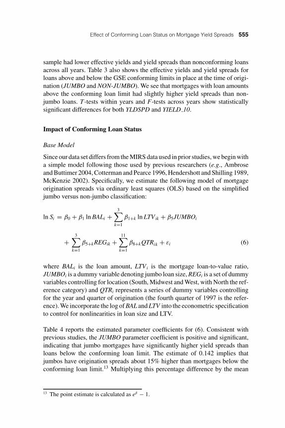
2004 V32 4: pp. 541–569

REAL ESTATE

ECONOMICS

The Effect of Conforming Loan Statuson Mortgage Yield Spreads: A LoanLevel AnalysisBrent W. Ambrose,∗ Michael LaCour-Little∗∗ and Anthony B. Sanders∗∗∗

The magnitude of the effect of government-sponsored enterprise purchaseson primary mortgage market rates has been a difficult research question withdiffering data and competing methodologies producing varying results. Herewe present a new approach using loan level data and controlling for credit riskdifferentials between conforming and nonconforming loans. Our method alsoaddresses econometric problems of endogeneity and sample selection bias.We find that conforming loans have yield spreads about 5.5% lower comparedto other loans on a risk-adjusted basis. This is lower than previous estimatesappearing in the literature.

Lenders in the primary mortgage market originate a range of contracts, manyof which are then sold in the secondary market, either to the government-sponsored enterprises (Fannie Mae and Freddie Mac, hereafter the GSEs1) orpooled as collateral for private label mortgage-backed securities. Other loans areretained in portfolio or sold on a whole-loan basis. Loans vary in coupon, size,term, collateral and, of course, credit quality. Based on business strategy andrisk preferences, together with information obtained during the underwritingprocess, and considering rules and price signals from the secondary market,lenders make a hold-versus-sell decision. What factors determine that decision,and what is the overall effect on rates in the primary market?

These questions are among many that are crucial to evaluating the role of theGSEs, whose special status in the economy generates both costs and benefits(Sanders 2002). GSE purchases provide liquidity to primary lenders and perhapsstability to the overall mortgage market (Gonzalez-Rivera 2001, Naranjo and

∗Gatton College of Business and Economics, University of Kentucky, Lexington, KY40506-0053 or [email protected].

∗∗Wells Fargo Home Mortgage and Washington University, St. Louis, Clayton, MO63105 or [email protected].

∗∗∗Finance Department, The Ohio State University, Columbus, OH 43210 or [email protected].

1 There are other GSEs operating in the housing finance arena, including the FederalHome Loan Banks.

542 Ambrose, LaCour-Little and Sanders

Toevs 2002). In addition, it is widely accepted that GSE activity reduces rateson conforming loans by expanding available funds to lenders (Phillips 1996).But the extent to which the GSEs reduce mortgage rates is controversial.2 Forexample, Ambrose, Buttimer and Thibodeau (2001) show the impact of houseprice volatility on the jumbo/non-jumbo loan rate differential. Their simulationsindicate that as much as 20% of the loan rate differential may be due to houseprice volatility.

On the other hand, GSEs benefit from an implied federal guaranty of theirliabilities and are exempt from certain taxes and requirements that other financialintermediaries bear. A number of papers have examined the funding advantageof the GSE, most recently Ambrose and Warga (2002) and Nothaft, Pearceand Sevanovic (2002). The latter identifies seven prior studies, which providea range of estimates of the funding advantage of between 23 and 72 basispoints, depending on data used, comparison instrument and methodology, andthe authors provide their own estimate of 27–30 basis points. Ambrose andWarga provide a broader comparison across risk classes and estimate an averagefunding advantage of 25–29 basis points over “AA”-rated banking sector bonds,43–47 basis points over “A”-rated banking bonds and 76–80 basis points over“BBB”-rated banking sector bonds.

Our effort here again focuses on the benefit side of the ledger, that is, the ratereduction associated with conforming loan status. In contrast to research thatrelies on macro-level yield data, we return to the loan level approach as inHendershott and Shilling (1989). But our data are more recent and includeborrower credit score, a key piece of information that allows us to estimate thereduction in mortgage yield spreads attributable to conforming loan status ona risk-adjusted basis. In addition, we can more precisely separate conformingfrom nonconforming loans, a task that cannot be accomplished with the dataused by McKenzie (2002), Ambrose and Buttimer (2004) and Passmore, Sparksand Ingpen (2002).3 Finally, our approach corrects for two distinct econometricproblems: endogeneity and sample selection bias. Endogeneity occurs becausethe loan-to-value ratio is jointly determined with note rate. Sample selectionbias may occur because some loans that could be sold to the GSEs may not be.

2 A long line of research has addressed this question, including Hendershott and Shilling(1989), Ambrose and Warga (1995), Cotterman and Pierce (1996), Kolari, Fraser andAnari (1998), Roll (2000), Todd (2001), Gonzalez-Rivera (2001), Ambrose, Buttimerand Thibodeau (2001), Ambrose and Buttimer (2004), McKenzie (2002), Naranjo andToevs (2002) and Passmore, Sparks and Ingpen (2002).3 The MIRS data, which is a sample of actual loan prices, only allows separation ofloans into jumbo versus not-jumbo based on the conforming loan size limit, therebymissing most loans of conforming loan size which are ineligible for GSE purchase dueto credit factors.

Effect of Conforming Loan Status on Mortgage Yield Spreads 543

If the GSEs purchase lower risk loans, then a simple comparison of yields willbe confounded by any credit risk differential.

To address this question we develop an ex ante model of yield spreads con-trolling for credit risk at the loan level. The model incorporates a variety ofcharacteristics including credit score, borrower age and income and loan-to-value ratio (LTV). We also incorporate actual outcomes, that is, whether theloan was, in fact, sold into the secondary mortgage market or retained in port-folio by the originating lender, as well as bond market environmental factors.

The plan for the remainder of the paper is as follows. In the next section,we briefly review relevant literature, drawing analogies to the corporate bondmarket. In the second section, we sketch out the theory of mortgage valuationand develop our model of mortgage yield spreads. In the third section, wedescribe the data. The fourth section presents the basic regression model thatis comparable to the existing literature. We then refine the model to control forcredit risk and address econometric issues. The final section offers conclusions.

Literature Review

A number of studies have examined the conforming-nonconforming rate dif-ferential. In most cases rates on jumbo loans are taken as the relevant noncon-forming loan category, although the reality is that some conforming loan sizeloans are, in fact, nonconforming, due to credit or documentation issues (e.g.,subprime or low-doc loans). Most previous studies rely on the Federal HousingFinance Board’s monthly mortgage interest rate survey (MIRS), which onlyallows separation into jumbo versus non-jumbo categories and lacks impor-tant credit risk measures. McKenzie (2002) provides an excellent discussionof the issues associated with estimating the loan rate differential using theMIRS data. McKenzie also provides a summary of previous empirical esti-mates. Depending on the period examined and methodology employed, thejumbo/non-jumbo mortgage rate differential has ranged between a high of 60basis points (Cotterman and Pearce 1996) to a low of 8 basis points (Naranjoand Toevs 2002).

In one of the first studies using MIRS data, Hendershott and Shilling (1989)found that conforming loans had interest rates 24 to 39 basis points lowerthan nonconforming loans after controlling for loan characteristics. They re-gressed effective mortgage interest rate against a set of variables to controlfor jumbo loan status, loan size, loan-to-value ratio, new versus existing homestatus, as well as dummy variables to capture temporal and regional varia-tions. Subsequent studies (e.g., ICF Inc. 1990, Cotterman and Pearce 1996,Ambrose, Buttimer and Thibodeau 2001, U.S. Congressional Budget Office2001, McKenzie 2002, Naranjo and Toevs 2002, Passmore, Sparks and Ingpen


2002) have followed a similar methodology with minor variations in datascreens designed to isolate the conforming/nonconforming effect as well asgeographic differences (e.g., McKenzie 2002, Ambrose and Buttimer 2004).Todd (2001) follows the Hendershott and Shilling methodology adding in theeffect of origination costs using Freddie Mac and Federal Reserve aggregatedata. Naranjo and Toevs (2002) extend the Hendershott and Shilling method-ology to incorporate cointegration to correct for nonstationarity in rates.4

Studies of the determinants of yield spreads in the corporate bond literature havefocused on credit spreads (see Altman and Saunders 1998 for a review). Formortgages, credit risk has traditionally been viewed as a function of borrower eq-uity or loan-to-value ratio. Early research includes von Furstenberg (1969), vonFurstenberg and Green (1974), Campbell and Dietrich (1983) and Cunninghamand Capone (1990). Quercia and Stegman (1992) and Vandell (1993) providesurveys focusing on default, while Kau, Keenan and Kim (1994) develop theo-retical default given stochastic collateral values. Among recent methodologicalinnovations, Deng, Quigley and Van Order (2000) present a competing riskmodel of mortgage termination, both default and prepayment, accounting forunobserved borrower heterogeneity. Mortgage default research has also recentlybegun to incorporate borrower credit score (e.g., Avery et al. 1996). In a relatedline of research outside of the mortgage literature, Angbazo, Mei and Saunders(1998) examine yield spreads for highly leveraged corporate loans.

Linking the mortgage literature to the broader finance literature, yield spreadson the firm’s debt reflect underlying financial risk that depends on firm capitalstructure, just as default risk in mortgages is related to the borrower’s equity.Likewise, we may think of borrower credit score as the analog to firm creditrating and individual borrower demographic characteristics as the analog tofirm specific idiosyncratic risk factors.

Theoretical Predications and Model

The general approach to mortgage pricing is now well established. Mortgagesare contingent claims contracts in which the mortgage value (VM) dependscritically on two stochastic processes, the market interest rate, r(t), and thehouse value, H(t). For instance, we may specify the interest rate process with aCIR diffusion process:

d(r ) = γ (� − r ) dt + σr√

r dzr , (1)

4 Kolari, Fraser and Anari (1998) also utilize cointegration methods to investigate theimpact of securitization on mortgage yield spreads using data from MIRS. However,their analysis does not examine the differential between conforming and nonconformingloans.


where � is the steady-state mean rate, γ is the speed of adjustment factor and σr

is the volatility of interest rates.5 Diffusion in collateral value affects mortgagevalue, too, so we may specify the evolution of house values, H(t), by

dH

H= (α − s) dt + σH dzH , (2)

where α is the instantaneous total return to housing, s is the service flow andσH is the volatility of housing returns. In (1) and (2), dzr and dzH are standardWiener processes and the correlation between the movements of the two statevariables (dzH and dzr)) is ρ.

Kau and Keenan (1995) show that under appropriate assumptions, the valueof the mortgage (VM) will satisfy the following partial differential equation(PDE):

1

2H 2σ 2

H

∂2V M

∂H 2+ ρH

√rσHσr

∂2V M

∂H∂r+ 1

2rσ 2

r

∂2V M

∂r2

+ γ (θ − r )∂V M

∂r+ (r − s)H

∂V M

∂H+ ∂V M

∂t− rV M = 0. (3)

Specifying the boundary conditions allows the valuation of the mortgage whenthe economic variables take on extreme values. With these boundary conditions,(3) can be solved to find the value of the mortgage contract.

We denote the present value of the remaining mortgage payments as A(r(t), t).Since house prices and interest rates interact in determining the value of theright to terminate the mortgage, J(r(t), H(t), t), the mortgage value is givenas

V M (r (t), H (t), t) = A(r (t), t) − J (r (t), H (t), t). (4)

The right to terminate the mortgage is composed of the right to prepay themortgage and the right to default.6 Standard comparative statics show that∂V M/∂σH < 0, ∂V M/∂σr < 0 and ∂V M/∂H > 0.7 Assuming that VM representsthe mortgage value at origination (net of any discount points), then the yield

5 Equation (1) is the standard Cox, Ingersoll and Ross (1985) interest rate model.6 Kau, Keenan and Kim (1993, 1994) show that the option pricing technique can beutilized to determine the probability of default.7 See Kau, Keenan, Muller and Epperson (1992, 1993) for a complete discussion of thefixed-rate mortgage contract comparative statics.


(yM) is simply the internal rate of return that equates the expected mortgagepayments (principal and interest) over the expected holding period to VM .8

Following Merton (1974), we define the mortgage credit risk premium as thedifference between the yield and the risk-free rate (yM − r), where the Treasurybond rate serves as a proxy for the risk-free rate. Although Merton examinedthe relationship between the risk premium on discount debt issued by a firm, thecomparative statics from the mortgage pricing model (4) and Merton’s analysisof risky debt imply that the yield spread (yM − r) is a function of the volatilityof the underlying state variables (house values and interest rates) as well as theloan-to-value ratio at origination (VM (r (0), H (0), 0)/H (0)). Thus, consistentwith Merton, we have that

∂S/∂σH > 0, ∂S/∂σr > 0, and ∂S/∂(V M (r (0), H (0), 0)/H (0)) > 0

where S = (yM − r).

Many models of yield spreads have been developed in the corporate bond marketfollowing Merton (1974).9 For example, Bakshi, Madan and Zhang (2000) testfor the presence of firm-specific distress factors in discount rate models forcorporate bonds. Results confirm that firm-specific factors (such as leverageand book-to-market ratios) as well as market interest rates explain differencesin corporate bond yields. We follow this example and propose the followinggeneralized model of the yield spread (S):

ln Si = α0 + α1σHi + α2σri + α3(V m

i

/Hi

) + α4CONFORMi

+ α5 Xi +11∑

j=1

δj QTR ji + εi (5)

where CONFORMi is a dummy variable denoting mortgages that meet the GSEconforming guidelines, Xi represents a vector of borrower-specific and marketfactors that may impact yield spreads, YRi is a dummy variable denoting theyear of origination and MONi is a dummy variable denoting the month oforigination.10 Including the dummy variable CONFORM in (5) sets up our test

8 In the empirical analysis, we assume a 10-year expected holding period rather thanthe full 30-year mortgage term.9 For example, see Duffie (1998, 1999), Collin-Dufresne, Goldstein and Martin (2001),Duffie and Singleton (1999), Bakshi, Madan and Zhang (2000) and Ericsson and Renault(2000).10 We include the yearly dummy variable to capture any variation in market creditconditions not specifically identified. We include the monthly dummy variable to captureany seasonal effects associated with mortgage origination.


of whether origination spreads are lower for loans that are eligible for GSEpurchase compared to those which are not.

Data

Data used for this research consist of origination records on 26,179 conven-tional fixed-rate mortgages made between January 1995 and December 1997by a national lender, the lender’s correspondent lenders and mortgage bro-kers. Both conforming and nonconforming loans are included, although super-jumbos (loans with initial balances in excess of $650,000) are not. Table 1reports the distribution of the loans by origination year and geography. We alsocompare the distribution of loans to the MIRS and Home Mortgage DisclosureAct (HMDA) databases for 1997 to ensure that our data are reasonably repre-sentative. Cross-sectionally, our sample is somewhat overrepresented by loansin New York/New Jersey and underrepresented in the Northwest and Southwestregions. However, the distribution of mortgage originations across years doesfollow the same pattern as that observed in the broader market.

We have relatively complete micro-level data for each loan in the sample. Inaddition to geography, loan amount and note rate, we observe points paid atthe time of loan origination so we can correctly compute yields over a givenhorizon. Major credit quality indicators, loan-to-value ratio (LTV) and borrowercredit score at time of origination (FICO), are also available, as is whether theloan had private mortgage insurance. Borrower demographic characteristicsavailable include age (BRWAGE) and income (INCOME). Table 2 reports thedescriptive statistics (mean, median and standard deviation) for the sample byorigination year. Across all origination years, the mean LTV is 75.6%. About69% have LTVs below 80%, 15% have LTVs between 80% and 90% and 16%have LTVs greater than 90% (see Table 2).

Across time, credit quality appears to have increased, with declining LTVs andincreasing credit scores. The average FICO score increased from 715 in 1995to 722 in 1997 and averaged 720 over the full sample. Average borrower age atorigination (our proxy for wealth) increased from 40 years in 1995 to 42 yearsin 1997 and average borrower income at origination increased from $62,510 in1995 to $87,960 in 1997. Consistent with housing market appreciation and amore affluent borrower pool, loan amounts increased over time from $107,700in 1995 to $141,500 in 1997.

Our data contain both conforming and nonconforming loans; however, while weobserve outcomes (i.e., whether sold to Fannie Mae or Freddie Mac, sold into aprivate label MBS or retained in portfolio), we cannot precisely determine loanstatus at origination. About 71% of the loans were actually sold to the agencies

548 Ambrose, LaCour-Little and SandersTa

ble

1�

Dis

trib

utio

nof

mor

tgag

elo

ans

byor

igin

atio

nye

aran

dlo

catio

n.

Sam

ple

MIR

SH

MD

A19

9519

9619

97A

llY

ears

1995

1996

1997

All

Yea

rs19

97%

Tota

l%

Tota

l%

Tota

l%

of%

Tota

l%

Tota

l%

Tota

l%

of%

Tota

lY

ear

Yea

rY

ear

Tota

lY

ear

Yea

rY

ear

Tota

lY

ear

Reg

ion

1:N

ewE

ngla

ndC

T1.

7%2.

3%2.

7%2.

4%2.

0%1.

9%1.

2%1.

6%1.

18%

ME

0.3%

0.2%

0.2%

0.2%

0.3%

0.3%

0.3%

0.3%

0.35

%M

A1.

2%1.

5%2.

0%1.

7%1.

8%2.

1%2.

2%2.

1%2.

38%

NH

0.4%

0.2%

0.3%

0.3%

0.3%

0.3%

0.3%

0.3%

0.40

%R

I0.

2%0.

1%0.

1%0.

1%0.

1%0.

1%0.

1%0.

1%0.

33%

VT

0.1%

0.1%

0.1%

0.1%

0.2%

0.2%

0.1%

0.2%

0.18

%To

tal

4.0%

4.4%

5.4%

4.8%

4.7%

4.9%

4.3%

4.6%

4.82

%

Reg

ion

2:N

ewY

ork/

New

Jers

eyN

J6.

5%6.

4%5.

5%6.

0%3.

3%3.

7%3.

9%3.

7%4.

05%

NY

23.7

%33

.2%

22.2

%25

.1%

2.9%

2.5%

2.0%

2.4%

2.71

%To

tal

30.2

%39

.5%

27.7

%31

.0%

6.2%

6.2%

6.0%

6.1%

6.76

%

Reg

ion

3:M

id-A

tlant

icD

E0.

2%0.

4%0.

2%0.

2%0.

5%0.

5%0.

5%0.

5%0.

31%

DC

0.7%

0.7%

0.8%

0.7%

0.1%

0.1%

0.2%

0.2%

0.19

%M

D3.

2%2.

8%4.

0%3.

5%2.

6%2.

6%2.

4%2.

5%1.

94%

PA2.

9%2.

2%2.

0%2.

2%5.

9%5.

2%3.

8%4.

8%4.

15%

VA

1.9%

2.7%

3.2%

2.7%

3.2%

3.1%

3.4%

3.2%

2.40

%W

V0.

1%0.

1%0.

1%0.

1%0.

2%0.

2%0.

2%0.

2%0.

43%

Tota

l8.

9%8.

8%10

.3%

9.6%

12.5

%11

.7%

10.5

%11

.4%

9.42

%

Reg

ion

4:So

uthe

ast

AL

0.4%

1.2%

1.0%

0.9%

0.6%

0.6%

0.5%

0.5%

1.37

%FL

6.3%

7.4%

5.6%

6.2%

7.8%

7.4%

5.7%

6.9%

6.40

%G

A1.

2%1.

1%1.

4%1.

3%1.

5%1.

6%1.

9%1.

7%3.

06%


KY

0.3%

0.2%

0.2%

0.2%

0.9%

0.8%

0.8%

0.8%

1.37

%M

S0.

1%0.

1%0.

1%0.

1%0.

5%0.

5%0.

4%0.

4%0.

85%

NC

1.4%

1.7%

2.1%

1.9%

3.0%

3.0%

3.1%

3.0%

3.20

%SC

0.5%

0.4%

0.5%

0.4%

1.6%

1.9%

1.6%

1.7%

1.60

%T

N0.

8%0.

9%0.

5%0.

7%1.

3%1.

0%1.

2%1.

2%1.

88%

Tota

l11

.1%

13.0

%11

.3%

11.7

%17

.1%

16.8

%15

.2%

16.2

%19

.72%

Reg

ion

5:M

idw

est

IL11

.0%

9.5%

8.7%

9.5%

6.9%

5.8%

4.5%

5.6%

5.25

%IN

0.5%

0.3%

0.4%

0.4%

1.9%

1.9%

1.8%

1.9%

2.59

%M

I1.

2%1.

0%1.

0%1.

0%3.

3%3.

2%2.

4%2.

9%5.

12%

MN

0.6%

0.7%

0.7%

0.7%

0.7%

0.8%

2.9%

1.6%

1.98

%O

H1.

9%0.

8%2.

1%1.

8%4.

8%4.

6%4.

2%4.

5%4.

96%

WI

0.2%

0.1%

0.1%

0.1%

3.7%

3.6%

3.5%

3.6%

2.34

%To

tal

15.4

%12

.4%

13.0

%13

.5%

21.4

%19

.9%

19.3

%20

.1%

22.2

4%

Reg

ion

6:So

uthw

est

AR

0.7%

0.4%

0.4%

0.5%

0.2%

0.2%

0.3%

0.2%

0.69

%L

A0.

3%0.

2%0.

3%0.

3%0.

4%0.

4%0.

4%0.

4%1.

29%

NM

0.3%

0.4%

0.6%

0.5%

0.3%

0.3%

0.5%

0.4%

0.66

%O

K0.

4%0.

4%0.

4%0.

4%0.

6%0.

6%0.

6%0.

6%0.

87%

TX

2.7%

1.6%

2.2%

2.2%

6.2%

6.1%

5.1%

5.7%

4.70

%To

tal

4.5%

3.1%

3.9%

3.8%

7.7%

7.7%

6.9%

7.4%

8.22

%

Reg

ion

7:G

reat

Plai

nsIA

0.5%

0.3%

0.5%

0.5%

0.6%

0.7%

1.3%

0.9%

0.86

%K

S0.

5%0.

4%0.

8%0.

6%1.

1%1.

7%1.

3%1.

3%0.

82%

MO

4.2%

2.0%

2.1%

2.6%

2.5%

2.4%

1.6%

2.1%

2.10

%N

E0.

1%0.

0%0.

0%0.

0%0.

4%0.

5%0.

6%0.

5%0.

49%

Tota

l5.

3%2.

7%3.

4%3.

7%4.

6%5.

2%4.

8%4.

9%4.

26%

Reg

ion

8:R

ocky

Mou

ntai

nC

O0.

8%0.

9%1.

4%1.

1%1.

7%1.

7%2.

8%2.

2%2.

62%

MT

0.0%

0.0%

0.0%

0.0%

0.1%

0.2%

0.4%

0.3%

0.27

%N

D0.

0%0.

0%0.

0%0.

0%0.

0%0.

1%0.

2%0.

1%0.

13%

550 Ambrose, LaCour-Little and SandersTa

ble

1�

cont

inue

d.

Sam

ple

MIR

SH

MD

A19

9519

9619

97A

llY

ears

1995

1996

1997

All

Yea

rs19

97%

Tota

l%

Tota

l%

Tota

l%

of%

Tota

l%

Tota

l%

Tota

l%

of%

Tota

lY

ear

Yea

rY

ear

Tota

lY

ear

Yea

rY

ear

Tota

lY

ear

SD0.

2%0.

2%0.

1%0.

1%0.

1%0.

0%0.

3%0.

2%0.

20%

UT

0.6%

0.3%

0.4%

0.5%

0.2%

0.4%

1.0%

0.6%

1.26

%W

Y0.

0%0.

0%0.

0%0.

0%0.

1%0.

0%0.

2%0.

1%0.

16%

Tota

l1.

7%1.

5%2.

0%1.

8%2.

3%2.

4%4.

9%3.

4%4.

64%

Reg

ion

9:Pa

cific

AZ

0.0%

0.0%

0.0%

0.0%

2.2%

2.0%

2.7%

2.3%

2.29

%C

A14

.5%

12.0

%18

.4%

16.0

%13

.2%

13.7

%14

.1%

13.7

%11

.47%

HI

0.0%

0.0%

0.0%

0.0%

0.5%

0.5%

0.5%

0.5%

0.31

%N

V2.

2%1.

1%1.

3%1.

5%1.

5%1.

4%1.

4%1.

4%0.

89%

Tota

l16

.7%

13.2

%19

.8%

17.5

%17

.3%

17.6

%18

.7%

18.0

%14

.96%

Reg

ion

10:N

orth

wes

tA

K1.

0%0.

7%1.

4%1.

1%0.

0%0.

0%0.

1%0.

1%0.

12%

ID0.

0%0.

0%0.

1%0.

1%0.

3%0.

4%0.

6%0.

4%0.

48%

OR

0.5%

0.2%

0.5%

0.4%

2.1%

2.4%

2.8%

2.5%

1.70

%W

A0.

7%0.

4%1.

2%0.

9%3.

7%4.

7%6.

0%4.

9%2.

66%

Tota

l2.

2%1.

4%3.

2%2.

6%6.

1%7.

5%9.

5%7.

9%4.

95%

Tota

l#6,

600

6,03

013

,549

26,1

7912

8,78

213

3,45

818

3,05

244

5,29

27,

796,

111

Thi

sta

ble

repo

rts

the

freq

uenc

ydi

stri

butio

nby

year

and

loca

tion

for

the

sam

ple

of26

,179

conv

entio

nal

fixed

-rat

em

ortg

age

loan

sor

igin

ated

betw

een

Janu

ary

1995

and

Dec

embe

r19

97.

Bot

hco

nfor

min

gan

dno

ncon

form

ing

loan

sar

ein

clud

ed,

alth

ough

supe

r-ju

mbo

s(l

oans

with

initi

alba

lanc

esin

exce

ssof

$650

,000

)ar

eno

t.Fo

rco

mpa

riso

n,w

eal

sore

port

the

dist

ribu

tion

oflo

ans

inth

eM

ortg

age

Inte

rest

Rat

eSu

rvey

(MIR

S)co

mpi

led

byth

eFe

dera

lHou

sing

Fina

nce

Boa

rdan

dth

edi

stri

butio

nof

alll

oans

repo

rted

inth

e19

97H

ome

Mor

tgag

eD

iscl

osur

eA

ct(H

MD

A)

data

base

.


Tabl

e2

�D

escr

iptiv

est

atis

tics

(sta

ndar

dde

viat

ions

repo

rted

inpa

rent

hese

s).

Full

Sam

ple

1995

1996

1997

(N=

1428

5)(N

=46

95)

(N=

3265

)(N

=63

25)

Dif

fere

nce

inM

eans

Var

iabl

eL

abel

Med

ian

Mea

nM

edia

nM

ean

Med

ian

Mea

nM

edia

nM

ean

F-t

est

YIE

LD

Eff

ectiv

eyi

eld

(YT

M)

7.87

57.

913

8.01

58.

123

8.14

78.

108

7.65

37.

725

2369

.7∗∗

∗

(0.4

89)

(0.5

46)

(0.4

57)

(0.3

88)

YIE

LD

10E

ffec

tive

yiel

d(1

0yr

hold

)7.

875

7.93

78.

030

8.15

08.

186

8.13

57.

678

7.74

525

43.1

∗∗∗

(0.4

84)

(0.5

40)

(0.4

49)

(0.3

80)

YL

DSP

DY

IEL

D10

–10-

yr1.

604

1.62

51.

820

1.81

51.

610

1.61

11.

530

1.53

814

78.8

∗∗∗

Tre

asur

yra

te(0

.355

)(0

.397

)(0

.357

)(0

.290

)LT

VA

vera

geLT

V0.

797

0.75

60.

800

0.78

30.

796

0.75

20.

783

0.74

413

5.7∗∗

∗

(0.1

63)

(0.1

71)

(0.1

62)

(0.1

58)

LTV

80LT

V≤

80%

1.00

00.

685

1.00

00.

561

1.00

00.

696

1.00

00.

740

348.

1∗∗∗

(0.4

65)

(0.4

96)

(0.4

60)

(0.4

38)

LTV

8090

LTV

>80

%an

dLT

V≤

90%

0.00

00.

152

0.00

00.

155

0.00

00.

164

0.00

00.

145

6.2∗∗

(0.3

59)

(0.4

96)

(0.4

60)

(0.4

38)

LTV

9095

LTV

>90

%an

dLT

V≤

95%

0.00

00.

125

0.00

00.

230

0.00

00.

098

0.00

00.

087

471.

2∗∗∗

(0.3

31)

(0.4

21)

(0.2

97)

(0.2

81)

LTV

95LT

V>

95%

0.00

00.

038

0.00

00.

054

0.00

00.

042

0.00

00.

028

47.2

∗∗∗

(0.1

91)

(0.2

27)

(0.2

01)

(0.1

66)


Tabl

e2

�co

ntin

ued.

Full

Sam

ple

1995

1996

1997

(N=

1428

5)(N

=46

95)

(N=

3265

)(N

=63

25)

Dif

fere

nce

inM

eans

Var

iabl

eL

abel

Med

ian

Mea

nM

edia

nM

ean

Med

ian

Mea

nM

edia

nM

ean

F-t

est

FIC

OFa

irIs

aac

cred

itsc

ore

730.

000

720.

359

725.

000

715.

833

731.

000

721.

815

733.

000

721.

915

33.7

∗∗∗

(56.

726)

(59.

268)

(55.

496)

(55.

883)

BR

WA

GE

Bor

row

erag

e39

.000

41.5

0138

.000

40.2

5840

.000

41.6

9840

.000

42.0

1854

.3∗∗

∗

(11.

307)

(11.

317)

(11.

337)

(11.

244)

INC

OM

EB

orro

wer

inco

me

62.1

4879

.592

51.6

6062

.510

62.4

9679

.478

69.8

2887

.963

160.

8∗∗∗

(96.

773)

(51.

498)

(87.

206)

(114

.922

)O

RIB

AL

Loa

nam

ount

128,

000

153,

934

107,

700

121,

871

128,

000

152,

679

141,

500

170,

111

570.

5∗∗∗

(99,

023)

(73,

496)

(97,

332)

(106

,473

)A

GE

NC

Y1

=or

igin

ated

for

1.00

00.

709

1.00

00.

693

1.00

00.

727

1.00

00.

709

8.3∗∗

∗

sale

toag

ency

(0.4

54)

(0.4

61)

(0.4

45)

(0.4

54)

PO

RT

FO

LIO

1=

orig

inat

edfo

r0.

000

0.03

00.

000

0.06

10.

000

0.02

80.

000

0.01

614

7.5∗∗

∗

reta

ined

port

folio

(0.1

70)

(0.2

39)

(0.1

64)

(0.1

24)

PV

TL

AB

EL

1=

orig

inat

edas

0.00

00.

261

0.00

00.

245

0.00

00.

245

0.00

00.

275

14.6

∗∗∗

priv

ate

labe

lmbs

(0.4

39)

(0.4

30)

(0.4

30)

(0.4

47)

CO

NF

OR

M1

=co

nfor

min

glo

an1.

000

0.75

51.

000

0.76

01.

000

0.77

81.

000

0.74

215

.5∗∗

∗

(0.4

30)

(0.4

27)

(0.4

15)

(0.4

37)

Thi

sta

ble

repo

rts

the

desc

ript

ive

stat

istic

sfo

rth

esa

mpl

eof

26,1

79co

nven

tiona

lfix

ed-r

ate

mor

tgag

elo

ans

orig

inat

edbe

twee

nJa

nuar

y19

95an

dD

ecem

ber

1997

.Bot

hco

nfor

min

gan

dno

ncon

form

ing

loan

sar

ein

clud

ed,a

lthou

ghsu

per-

jum

bos

(loa

nsw

ithin

itial

bala

nces

inex

cess

of$6

50,0

00)

are

not.

Loa

nsw

ere

orig

inat

edth

roug

hout

the

Uni

ted

Stat

es.∗∗

∗ sig

nific

anta

tthe

1%le

vel,

∗∗si

gnifi

cant

atth

e5%

leve

l,∗ s

igni

fican

tat

the

10%

leve

l.


(Fannie Mae and Freddie Mac), 26% were sold as private label MBS and 3%were retained in portfolio. It seems reasonable to assume that loans actuallysold to the GSEs were conforming at origination and that jumbo loans werenot. The question is whether the small number of conforming-size loans thatwere not sold to the GSEs could have been. We use some admittedly arbitrarycriteria to make this determination. Since mortgages to borrowers with creditscores lower than 620 are classified by regulatory agencies as “subprime” andnot usually purchased by the GSEs without significant credit enhancement,we use this value as one credit quality cutoff. We then classify a mortgage asconforming if (1) the loan was sold to one of the GSEs, (2) the borrower FICOscore at origination is above 620, the loan amount was below the conformingloan limit in place at time of origination and the LTV is less than 80% or (3)the borrower FICO score at origination is above 620, the loan amount wasbelow the conforming loan limit in place at time of origination and the loanhas private mortgage insurance if the LTV is greater than 80%.11 Based on thisclassification scheme, we see that approximately 80% of the mortgages wereconforming loans at origination and were thus eligible for sale to the agencies.Hence, by our calculations, about 90% of conforming production was ultimatelysold to the GSEs.12

Table 2 reports the mean (and median) yield and yield spreads for the sample. Wereport both the effective yield-to-maturity (YIELD) as well as the effective yieldassuming a 10-year expected holding period (YIELD 10). The effective yieldcontrols for any points paid by the borrower at origination. In the subsequentanalysis, we use YIELD 10 since most loans are repaid prior to maturity. Theyield spread (YLDSPD) is calculated as the difference between the effectiveyield assuming a 10-year holding period and the then current 10-year Treasury.The data show a general downward drift in the effective yield and yield spreadsmirroring overall rate movements from 1995 to 1997.

We begin our analysis of the difference between conforming and nonconform-ing yield spreads with the simple nonparametric comparison shown simply inTable 3. We show the mean and median effective yield and yield spread forconforming and nonconforming loans assuming a 10-year expected holdingperiod. Consistent with previous empirical studies, conforming loans in our

11 We also estimated the credit spread models using a credit score of 660 to denoteconforming status. Overall, results remained consistent and do not appear to be sensitiveto our choice of credit score cutoff.12 Unfortunately, our classification scheme does not control for nonborrower creditquality underwriting criteria and thus may lead to some loans that are nonconformingdue to property characteristics being incorrectly categorized as conforming. While thenumber of these cases is probably small, the effect will be to bias down the conform-ing/nonconforming differential.


Tabl

e3

�M

ean

effe

ctiv

eyi

eld

and

yiel

dsp

read

sby

orig

inat

ion

year

,seg

men

ted

byco

nfor

min

g/no

ncon

form

ing

and

jum

bo/n

on-j

umbo

stat

us(s

tand

ard

devi

atio

nsre

port

edin

pare

nthe

ses)

.

1995

1996

1997

F-te

st

NY

LD

SPD

YIE

LD

10N

YL

DSP

DY

IEL

D10

NY

LD

SPD

YIE

LD

10Y

LD

SPD

YIE

LD

10

Con

form

ing

5,01

61.

789

8.06

64,

694

1.59

68.

124

10,0

601.

533

7.72

297

4.0∗∗

∗17

15.1

∗∗∗

(0.3

83)

(0.5

10)

(0.3

63)

(0.4

63)

(0.2

90)

(0.3

92)

Non

conf

orm

ing

1,58

41.

897

8.41

71,

336

1.66

78.

175

3,48

91.

550

7.81

154

9.3∗∗

∗12

17.6

∗∗∗

(0.4

26)

(0.5

44)

(0.3

27)

(0.3

97)

(0.2

92)

(0.3

33)

T-t

est

8.93

∗∗∗

22.7

∗∗∗

6.88

∗∗∗

4.04

∗∗∗

2.91

∗∗∗

12.9

9∗∗∗

Jum

bo53

01.

844

8.23

61,

233

1.66

58.

164

3,26

41.

544

7.80

123

9.2∗∗

∗64

2.8∗∗

∗

(0.3

84)

(0.5

09)

(0.3

02)

(0.3

78)

(0.2

69)

(0.3

03)

Non

-jum

bo6,

070

1.81

38.

143

4,79

71.

598

8.12

810

,285

1.53

67.

728

1237

.4∗∗

∗20

12.6

∗∗∗

(0.3

98)

(0.5

42)

(0.3

68)

(0.4

66)

(0.2

97)

(0.4

00)

T-t

est

−1.8

0∗−4

.02∗∗

∗−6

.72∗∗

∗−2

.89∗∗

∗−1

.56

−11.

10∗∗

∗

∗∗∗ s

igni

fican

tatt

he1%

leve

l,∗∗

sign

ifica

ntat

the

5%le

vel,

∗ sig

nific

anta

tthe

10%

leve

l.


sample had lower effective yields and yield spreads than nonconforming loansacross all years. Table 3 also shows the effective yields and yield spreads forloans above and below the GSE conforming limits in place at the time of origi-nation (JUMBO and NON-JUMBO). We see that mortgages with loan amountsabove the conforming loan limit had slightly higher yield spreads than non-jumbo loans. T-tests within years and F-tests across years show statisticallysignificant differences for both YLDSPD and YIELD 10.

Impact of Conforming Loan Status

Base Model

Since our data set differs from the MIRS data used in prior studies, we begin witha simple model following those used by previous researchers (e.g., Ambroseand Buttimer 2004, Cotterman and Pearce 1996, Hendershott and Shilling 1989,McKenzie 2002). Specifically, we estimate the following model of mortgageorigination spreads via ordinary least squares (OLS) based on the simplifiedjumbo versus non-jumbo classification:

ln Si = β0 + β1 ln BALi +3∑

k=1

β1+k ln LTVik + β5JUMBOi

+3∑

k=1

β5+kREGik +11∑

k=1

β8+kQTRik + εi (6)

where BALi is the loan amount, LTVi is the mortgage loan-to-value ratio,JUMBOi is a dummy variable denoting jumbo loan size, REGi is a set of dummyvariables controlling for location (South, Midwest and West, with North the ref-erence category) and QTRi represents a series of dummy variables controllingfor the year and quarter of origination (the fourth quarter of 1997 is the refer-ence). We incorporate the log of BAL and LTV into the econometric specificationto control for nonlinearities in loan size and LTV.

Table 4 reports the estimated parameter coefficients for (6). Consistent withprevious studies, the JUMBO parameter coefficient is positive and significant,indicating that jumbo mortgages have significantly higher yield spreads thanloans below the conforming loan limit. The estimate of 0.142 implies thatjumbos have origination spreads about 15% higher than mortgages below theconforming loan limit.13 Multiplying this percentage difference by the mean

13 The point estimate is calculated as eβ − 1.


Table 4 � OLS regression estimates for the base yield spread model and the adjustedmodel controlling for “conforming” loan status and borrower credit quality.

Model 1 Model 2

Variable Label Coeff. Std. Err. Coeff. Std. Err.

INTERCEPT Intercept 1.828∗∗∗ 0.036 3.468∗∗∗ 0.114CONFORM 1 = conforming loan −0.032∗∗∗ 0.006JUMBO 1 = jumbo loan 0.142∗∗∗ 0.005 0.113∗∗∗ 0.007Log(LTV) Log of loan-to-value ratio 0.036∗∗∗ 0.005 0.019∗∗∗ 0.005Log(FICO) Fair Isaac credit score −0.274∗∗∗ 0.015CREDITSPD AAA-BBB bond spread 0.684∗∗∗ 0.080Log(ORIBAL) Loan amount −0.118∗∗∗ 0.003 −0.114∗∗∗ 0.003HPI STDEV House price index 0.001∗ 0.001

volatilitySIG GS1 Interest rate volatility −0.225∗∗∗ 0.031YLDCURVE Yield curve slope −0.471∗∗∗ 0.017q2 Nonjudicial, no deficiency −0.024∗∗∗ 0.005q3 Judicial and deficiency 0.011∗∗∗ 0.003q4 Judicial, no deficiency −0.032∗ 0.020QTR95 1 1st quarter 1995 0.088∗∗∗ 0.010 0.444∗∗∗ 0.032QTR95 2 2nd quarter 1995 0.171∗∗∗ 0.006 0.402∗∗∗ 0.024QTR95 3 3rd quarter 1995 −0.005 0.005 0.159∗∗∗ 0.016QTR95 4 4th quarter 1995 0.183∗∗∗ 0.005 0.209∗∗∗ 0.016QTR96 1 1st quarter 1996 −0.123∗∗∗ 0.007 0.123∗∗∗ 0.019QTR96 2 2nd quarter 1996 −0.074∗∗∗ 0.006 0.196∗∗∗ 0.017QTR96 3 3rd quarter 1996 0.007 0.006 0.194∗∗∗ 0.015QTR96 4 4th quarter 1996 0.097∗∗∗ 0.006 0.232∗∗∗ 0.013QTR97 1 1st quarter 1997 −0.076∗∗∗ 0.008 0.104∗∗∗ 0.012QTR97 2 2nd quarter 1997 −0.063∗∗∗ 0.005 0.099∗∗∗ 0.009QTR97 3 3rd quarter 1997 −0.068∗∗∗ 0.004 0.040∗∗∗ 0.006SOUTH 1 = Located −0.033∗∗∗ 0.004 −0.024∗∗∗ 0.004

in South RegionMIDWEST 1 = Located 0.007∗ 0.004 0.003 0.004

in Midwest RegionWEST 1 = Located 0.001 0.003 0.023∗∗∗ 0.005Adjusted R2 in West Region 0.208 0.250

The dependent variable is the log of the origination yield spread, where the originationyield spread is calculated assuming a 10-year holding period. ∗∗∗significant at the 1%level, ∗∗significant at the 5% level, ∗significant at the 10% level.

sample yield spread of 162.5 basis points implies that jumbo loans have yieldspreads 24.8 basis points higher than non-jumbo loans. This result is completelyconsistent with other studies. For example, Hendershott and Shilling (1989)found that jumbo loan rates were 24 to 39 basis points higher than conformingloans, and, over the period from 1989 to 1993, Cotterman and Pearce (1996)estimated loan rate differentials between 24 and 60 basis points. Our result is


also consistent with McKenzie (2002), who estimates the jumbo/conformingloan rate differential between 11 and 31 basis points over the period from 1986to 2000, a longer period.

Base Model: Impact of Loan Risk Characteristics

The drawback to the base model of jumbo/non-jumbo spreads is that it doesnot control for loan risk characteristics and the fact that some conforming sizeloans may not actually be conforming. As a first step in addressing this prob-lem, Table 4 also reports an extended specification that includes borrower riskcharacteristics and other factors. We estimate this model over the full sample(1995 to 1997 originations) and include two indicator variables, CONFORMand JUMBO, to decompose the spread differential. This specification also in-cludes borrower credit score (FICO) and loan balance. To capture the time-varying market influences we also include the yield difference between the“AAA” bond index and the “Baa” bond index (CREDSPD) as well as a mea-sure of yield curve slope (YLDCURVE), proxied by the difference betweenthe 10-year and 1-year Treasury bond rates. Finally, following Ambrose andPennington-Cross (2000), we include a set of dummy variables that catego-rize states based on judicial versus nonjudicial foreclosure laws and deficiencyversus nondeficiency judgment states to control for differences in legal en-vironment. q1 indicates states that have nonjudicial foreclosure available andallow deficiency judgments;14 q2 indicates states that have nonjudicial fore-closure available and do not allow deficiency judgments;15 q3 indicates statesthat require judicial foreclosure and allow deficiency judgments16 and finallyq4 indicates states that require judicial foreclosure and do not allow deficiencyjudgments.17

Based on the theoretical model of yield spreads outlined above, we expect yieldspreads to be related to house price and interest rate volatility and loan-to-valueratio. We construct a proxy for house price volatility by calculating the standarddeviation in the OFHEO state-level house price index over the eight quartersprior to the quarter of origination. We use the standard deviation in the 1-yearTreasury bond rate over the 15 months prior to origination as a proxy for ratevolatility.

14 q1 indicate AL, AR, DC, GA, HI, MO, IA, MA, MD, MI, MS, RI, NE, NH, NM, NV,NY, TN, UT, VA, WV, WY and CO.15 q2 indicate AK, AZ, CA, ID, OK, ME, MN, MT, NC, OR, SD, TX and WA.16 q3 indicate CT, DE, FL, IL, IN, KS, KY, NJ, OH, PA, SC and VT.17 q4 indicate LA, ND and WI.


Results indicate that it is possible to decompose the 15% jumbo–non-jumbo dif-ferential into two distinct parts: an exogenous loan size effect and an endogenouscredit quality effect reflecting GSE underwriting. The positive and significantcoefficient for JUMBO measures the size effect: Loans exceeding the GSE con-forming loan limit have yield spreads 12.0% above loans with balances belowthe limit. The negative coefficient for CONFORM indicates that loans meetingthe conforming guidelines have yield spreads 3.2% lower than nonconformingloans. Again, multiplying these estimates by the sample mean suggests thatconforming loans have yield spreads that are 5.1 basis points lower than non-conforming, non-jumbo loans, while jumbo loans have yield spreads that are19.4 basis points above the nonconforming, non-jumbo segment and 24.5 basispoints above conforming loans.

We also note that adding borrower risk characteristics and incorporating marketrisk factors increases the model’s adjusted R2 from 20.8% to 25%. We now turnto additional econometric issues and further refinement of the model to addressthem.

Econometric Issues

Endongeneity

To reduce default risk, lenders impose LTV restrictions. However, since LTVis such an important component of underwriting, it can be argued that LTV,mortgage amount and contract rate are jointly determined. Moreover, the en-dogenous relationship between the level of mortgage debt and the amount ofhousing consumption is well known. For example, Ling and McGill (1998) de-velop a simultaneous equation model where mortgage demand is a function ofborrower income, nonhousing wealth, desired housing consumption and demo-graphic characteristics, and housing consumption is a function of the level ofmortgage debt as well as economic and demographic factors. To control for thisendogenous relationship, we specify LTV and house value as a simultaneousequations system and utilize the predicted loan-to-value (LTV) in the subse-quent yield spread regression. We estimate the following system via two-stageleast squares regression:

log(housei ) = β0 + β1LTVi + β2BRWAGEi + β3BRWAGE2i + β4rmkt

+β5INCOMEi + β6INCOME2i + β7YR95 + β8YR96

+10∑

k=2

β7+kREGi,k + εi (7)


LTVi = α0 + α1 log(housei ) + α2FICOi + α3rmkt + α4INCOMEi

+ α5INCOME2i + α6q2 + α7q3 + α8q4 + α9YR95 + α10YR96

+10∑

k=2

α9+kREGi,k + εi (8)

where INCOMEi is borrower i’s income at origination, BRWAGEi is borroweri’s age at origination, rmkt is the current mortgage rate at origination as proxiedby the Freddie Mac 30-year fixed-rate mortgage rate, FICOi is borrower i’scredit score at origination,18 YR95 and YR96 are dummy variables denotingyear of origination (1997 is the control year), and REGk (k = 1 . . . 4) are a seriesof dummy variables denoting the region where the loan is located (Region 1,North, is the control region). Use of borrower age and income together providesa rough proxy for total wealth, or permanent income, and we include the squareof these variables to control for any nonlinear effects in wealth or income. Wealso include the previously described set of dummy variables that classify statesbased legal environment (q1 . . . q4).

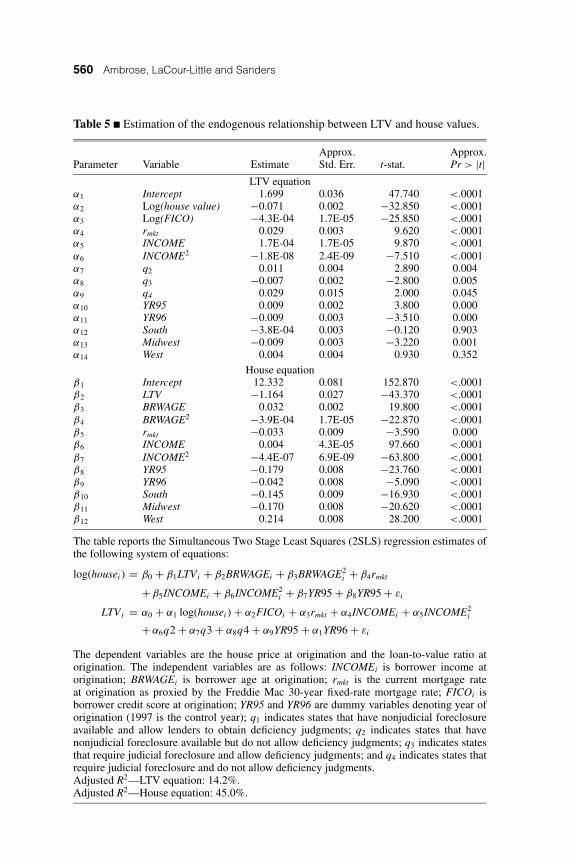
Table 5 reports the results of estimating Equations (7) and (8) via two-stage leastsquares. Consistent with Ling and McGill (1998), we find that loan-to-valueratios are lower for higher value homes and for borrowers with higher creditratings. We also find that borrower income is nonlinearly related to LTV, withindividuals having greater income capable of supporting higher LTV ratios. Wealso find that LTV ratios are higher in states that do not allow lenders to pursuedeficiency judgments (q2 and q4). Based on the model coefficients reported inTable 5, we calculate the predicted LTV ratio for each borrower, which is usedin the enhanced yield spread model.

Table 6 reports our enhanced yield spread model using the predicted LTV val-ues. The coefficient on CONFORM remains significantly negative, implyingthat conforming loans do have lower yield spreads than nonconforming loans.However, correcting for the endogenous relationship for LTV causes the mag-nitude of the conforming loan differential to shrink. The estimated coefficientin Table 6 implies that conforming loans have yield spreads that are 3.0%lower than nonconforming loans. Again, this implies that conforming loanshave yield spreads that are approximately 24.4 basis points smaller than jumboloans.

18 In the empirical estimation, we use the log of FICO.


Table 5 � Estimation of the endogenous relationship between LTV and house values.

Approx. Approx.Parameter Variable Estimate Std. Err. t-stat. Pr > |t|

LTV equationα1 Intercept 1.699 0.036 47.740 <.0001α2 Log(house value) −0.071 0.002 −32.850 <.0001α3 Log(FICO) −4.3E-04 1.7E-05 −25.850 <.0001α4 rmkt 0.029 0.003 9.620 <.0001α5 INCOME 1.7E-04 1.7E-05 9.870 <.0001α6 INCOME2 −1.8E-08 2.4E-09 −7.510 <.0001α7 q2 0.011 0.004 2.890 0.004α8 q3 −0.007 0.002 −2.800 0.005α9 q4 0.029 0.015 2.000 0.045α10 YR95 0.009 0.002 3.800 0.000α11 YR96 −0.009 0.003 −3.510 0.000α12 South −3.8E-04 0.003 −0.120 0.903α13 Midwest −0.009 0.003 −3.220 0.001α14 West 0.004 0.004 0.930 0.352

House equationβ1 Intercept 12.332 0.081 152.870 <.0001β2 LTV −1.164 0.027 −43.370 <.0001β3 BRWAGE 0.032 0.002 19.800 <.0001β4 BRWAGE2 −3.9E-04 1.7E-05 −22.870 <.0001β5 rmkt −0.033 0.009 −3.590 0.000β6 INCOME 0.004 4.3E-05 97.660 <.0001β7 INCOME2 −4.4E-07 6.9E-09 −63.800 <.0001β8 YR95 −0.179 0.008 −23.760 <.0001β9 YR96 −0.042 0.008 −5.090 <.0001β10 South −0.145 0.009 −16.930 <.0001β11 Midwest −0.170 0.008 −20.620 <.0001β12 West 0.214 0.008 28.200 <.0001

The table reports the Simultaneous Two Stage Least Squares (2SLS) regression estimates ofthe following system of equations:

log(housei ) = β0 + β1LTVi + β2BRWAGEi + β3BRWAGE2i + β4rmkt

+ β5INCOMEi + β6INCOME2i + β7YR95 + β8YR95 + εi

LTVi = α0 + α1 log(housei ) + α2FICOi + α3rmkt + α4INCOMEi + α5INCOME2i

+ α6q2 + α7q3 + α8q4 + α9YR95 + α1YR96 + εi

The dependent variables are the house price at origination and the loan-to-value ratio atorigination. The independent variables are as follows: INCOMEi is borrower income atorigination; BRWAGEi is borrower age at origination; rmkt is the current mortgage rateat origination as proxied by the Freddie Mac 30-year fixed-rate mortgage rate; FICOi isborrower credit score at origination; YR95 and YR96 are dummy variables denoting year oforigination (1997 is the control year); q1 indicates states that have nonjudicial foreclosureavailable and allow lenders to obtain deficiency judgments; q2 indicates states that havenonjudicial foreclosure available but do not allow deficiency judgments; q3 indicates statesthat require judicial foreclosure and allow deficiency judgments; and q4 indicates states thatrequire judicial foreclosure and do not allow deficiency judgments.Adjusted R2—LTV equation: 14.2%.Adjusted R2—House equation: 45.0%.


Table 6 � Adjusted model controlling for conforming, jumbo status and borrowercredit.

Model 3

Std.Variable Label Coeff. Err. T-stat. P-value

INTERCEPT Intercept 2.217 0.194 11.437 0.000CONFORM 1 = conforming loan −0.030 0.006 −5.411 0.000JUMBO 1 = jumbo loan 0.114 0.007 16.459 0.000Log(LTV) Log of loan-to-value ratio 0.373 0.046 8.120 0.000Log(FICO) Fair Isaac credit score −0.119 0.025 −4.719 0.000CREDITSPD AAA-BBB bond spread 0.694 0.080 8.727 0.000Log(ORIBAL) Loan amount −0.085 0.004 −19.560 0.000HPI STDEV House price index volatility 0.001 0.001 1.670 0.095SIG GS1 Interest rate volatility −0.235 0.031 −7.615 0.000YLDCURVE Yield curve slope −0.489 0.018 −27.880 0.000Q2 Nonjudicial, no deficiency −0.029 0.005 −5.744 0.000Q3 Judicial and deficiency 0.015 0.003 4.474 0.000Q4 Judicial, no deficiency −0.047 0.020 −2.408 0.016QTR95 1 1st quarter 1995 0.436 0.032 13.442 0.000QTR95 2 2nd quarter 1995 0.398 0.024 16.814 0.000QTR95 3 3rd quarter 1995 0.155 0.016 9.881 0.000QTR95 4 4th quarter 1995 0.205 0.016 13.189 0.000QTR96 1 1st quarter 1996 0.136 0.019 7.123 0.000QTR96 2 2nd quarter 1996 0.201 0.017 11.645 0.000QTR96 3 3rd quarter 1996 0.195 0.015 12.668 0.000QTR96 4 4th quarter 1996 0.237 0.013 17.840 0.000QTR97 1 1st quarter 1997 0.103 0.012 8.550 0.000QTR97 2 2nd quarter 1997 0.096 0.009 10.571 0.000QTR97 3 3rd quarter 1997 0.041 0.006 6.554 0.000SOUTH 1 = Located in South Region −0.025 0.004 −6.206 0.000MIDWEST 1 = Located in Midwest 0.007 0.004 1.684 0.092

RegionWEST 1 = Located in West Region 0.022 0.005 4.298 0.000Adjusted R2 0.251

Estimated with predicted LTVs.

Sample Selection Bias

As discussed previously, raw data suggests that conforming loan rates are con-sistently lower than nonconforming rates. But such a pattern could emerge forat least two distinct reasons. First, the differential could reflect a liquidity pre-mium, since it is less costly to sell (or swap) loans to the GSEs, comparedto the creating complex private label mortgage-backed securities. Second, thedifferential could be attributable to credit risk, that is, if the GSEs purchase onlyloans with lower credit risk, then any comparison to rates for higher risk loanswould be confounded by this difference.


To control for this potential sample selection bias, we estimate the “treatmenteffects” model (see Green 1997). This procedure involves estimating the fol-lowing conforming loan selection model:

CONFORMi = γZi + ξi , (9)

where Zi is a vector of characteristics that determines whether the loan is aconforming loan and ξ i is an error term. Since the GSEs have congression-ally mandated missions to increase the supply of mortgage credit for low-and moderate-income borrowers, we assume that Zi includes borrower income(INCOME) and age (BRWAGE, proxying for borrower wealth) along withdummy variables for year to reflect the yearly adjustments in the conform-ing loan limit. We estimate (9) as a probit model with the following form:

Pr(CONFORMi = 1) = φ(−γZi )

1 − �(−γZi )(10)

and

Pr(CONFORMi = 0) = [1 − Pr(CONFORMi = 1)], (11)

where φ is the standard normal probability density function (pdf) and � is thestandard normal cumulative distribution function (cdf). From the probit modelcoefficients, γ , we compute the inverse Mills ratio (λi) as

λi = φ(γZi )/�(γZi ). (12)

Flannery and Houston (1999) discuss that if εi and ξ i are jointly normallydistributed, then

E(εi | CONFORMi ) = ρσξ E(ξi | CONFORMi ), (13)

where ρ is the correlation between εi and ξ i, and σ ξ is the standard deviation ofξ i. Then in the second step, we reestimate Equation (5) via least squares withλi included as an explanatory variable:19

ln Si = α0 + α1σHi + α2σri + α3(V M

i

/Hi

) + α4CONFORMi

+ βXi +11∑

j=1

δj QTRji + ϕλi + εi (14)

19 The two-step estimation procedure follows Heckman (1979).


Table 7 � Sample selection correction.

Panel A: Probit modela

Parameter Estimate Error Chi Square Pr > ChiSq

INTERCEPT 2.451 0.080 946.740 <.0001BRWAGE 0.005 0.001 32.370 <.0001INCOME −0.008 0.000 3,308.890 <.0001Log(LTV) −1.727 0.071 591.960 <.0001YR95 −0.069 0.023 9.190 0.002YR96 0.088 0.023 14.380 0.000

The inverse Mills ratio coefficient (ϕ) is a measure of (ρσ ξ ) in (14); hence, if theparameter estimate of λ is zero, sample selection bias is not present. However,Willis and Rosen (1979) show that including λ corrects for selectivity bias in thesample observations. Furthermore, if the λ coefficient is statistically significant,then this suggests that the mortgage status as conforming impacts the mortgagespread at origination. Finally, following Flannery and Houston (1999), a positive(negative) ϕ implies that ρ > (<) 0, which suggests that the origination spreadon conforming loans is higher (lower) than nonconforming loans.

Table 7, Panel A presents the results of the first-stage probit model(Equation (9)). Results show that the probability of a loan being conforming ispositively related to borrower age and negatively related to borrower income.This result seems intuitive since older households would have accumulatedgreater funds for down payment and higher income households would be morelikely to purchase higher priced housing requiring jumbo loans. In addition, theprobability of being conforming declines as the loan-to-value ratio increases,consistent with underwriting of credit risk.

Table 7, Panel B presents the second-stage results with asymptotically correctedstandard errors for the yield spread model that includes the inverse-Mills ratioto control for sample selection bias. The significantly positive coefficient for λ

indicates that the loan spread is indeed affected by conforming loan status, fromwhich we may conclude that a simple OLS model of SPREAD without includingλ would suffer from omitted variables bias.20 In addition, since λ is positive,this implies that conforming loan origination spreads are actually larger thanwould be estimated under the simple OLS regression. In other words, the baseOLS coefficients presented in Tables 4 and 6 are biased.

20 See Flannery and Houston (1999) for a discussion of the interpretation of the inverse-Mills ratio in the context of the impact of bank examinations on market value.


Table 7 � continued.

Panel B: Second stage OLS regression with consistent asymptotic standard errorsb

Std.Variable Label Parameter Error T-stat. P-value

INTERCEPT Intercept 3.112 0.229 13.584 0.000CONFORM 1 = conforming loan −0.096 0.011 −9.143 0.000JUMBO 1 = jumbo Loan 0.107 0.007 15.443 0.000Log(FICO) Fair Isaac credit score −0.215 0.029 −7.555 0.000Log(LTV) Log of loan-to-value ratio 0.682 0.079 8.591 0.000CREDITSPD AAA-BBB bond spread −0.109 0.006 −19.995 0.000Log(ORIBAL) Loan amount 0.134 0.057 2.366 0.018HPI STDEV House price index volatility 0.001 0.001 1.581 0.114SIG GS1 Interest rate volatility −0.230 0.031 −7.454 0.000YLDCURVE Yield curve slope −0.478 0.018 −27.133 0.000q2 Nonjudicial, no deficiency −0.026 0.005 −5.180 0.000q3 Judicial and deficiency 0.013 0.003 3.785 0.000q4 Judicial, no deficiency −0.039 0.020 −1.971 0.049QTR95 1 1st quarter 1995 0.441 0.032 13.623 0.000QTR95 2 2nd quarter 1995 0.400 0.024 16.941 0.000QTR95 3 3rd quarter 1995 0.158 0.016 10.055 0.000QTR95 4 4th quarter 1995 0.207 0.016 13.364 0.000QTR96 1 1st quarter 1996 0.130 0.019 6.776 0.000QTR96 2 2nd quarter 1996 0.201 0.017 11.619 0.000QTR96 3 3rd quarter 1996 0.197 0.015 12.814 0.000QTR96 4 4th quarter 1996 0.237 0.013 17.840 0.000QTR97 1 1st quarter 1997 0.103 0.012 8.563 0.000QTR97 2 2nd quarter 1997 0.098 0.009 10.760 0.000QTR97 3 3rd quarter 1997 0.040 0.006 6.459 0.000SOUTH 1 = Located in South Region −0.025 0.004 −6.212 0.000MIDWEST 1 = Located in Midwest Region 0.004 0.004 1.046 0.295WEST 1 = Located in West Region 0.025 0.005 4.711 0.000λ Inverse Mill’s ratio 0.039 0.005 7.381 0.000

aThis panel reports the maximum-likelihood parameter estimates for the first-stage probitmodel of whether a loan is a conforming loan. The dependent variable is a dummyvariable equal to 1 if the loan is conforming and 0 otherwise. The independent variablesare as follows: INCOME is borrower income at origination; BRWAGE is borrower age atorigination; LTV is the actual loan-to-value ratio at origination; and YR95 and YR96 aredummy variables denoting year of origination (1997 is the control year).Log-likelihood: −12258.5.bThis panel reports the OLS regression estimates of the following equation:

ln Si = α0 + α1σHi + α2σri + α3(V M

i /Hi) + α1CONFORM

+ β Xi +11∑

j=1

δi QTR + ϕλi + εi

The dependent variable is the log of the yield spread calculated as the difference betweenthe effective loan yield assuming a 10-year holding period and the 10-year Treasury rate.The inverse Mills ratio (λ) is defined as λi = φ(γZi )/�(γZi )′, where γ are the parametercoefficients of the first-stage probit model reported in Panel A.


Other results are consistent with our expectations about the relationship betweenyield spreads and loan and borrower characteristics. Yield spreads are positivelyrelated to LTV and negatively related to borrower credit score. Furthermore,yield spreads are positively related to rate volatility.

Turning to the general macro-economic variables, we find that mortgage yieldspreads are negatively associated with changes in the general default risk pre-mium and negatively related to changes in the yield curve. The negative coeffi-cient for the bond market yield spread (CREDSPD) indicates that a 1 basis pointincrease in the corporate bond market yield spread results in a 1.2 basis pointdecrease in mortgage yield spreads (assuming a conforming loan with an LTVratio of 80%). Likewise, a 1 basis point increase in the yield curve translatesinto approximately a 0.7 basis point decline in the mortgage yield spread. Thelegal environment dummy variables indicate that loans originated in states thatdo not allow deficiency judgments have lower origination spreads. Given thatthese states have more borrower-friendly laws, it is rather surprising that thenegative coefficient suggests that loans originated in these states actually havelower yield spreads than loans originated in other more lender-friendly states.

Finally, the parameter estimate for the conforming loan dummy variable contin-ues to be negative and statistically significant while the estimate for the jumbosize dummy is positive and significant. The JUMBO coefficient indicates thatmortgages with loan amounts above the GSE conforming loan limit have yieldspreads that are on average approximately 11.3% higher than mortgages withloan amounts below the conforming loan limit. This implies that mortgagesabove the conforming loan limit have yield spreads that are 18.4 basis pointsabove loans that are below the conforming loan limit (evaluated at the averageyield spread of 162.5 basis points). Following Greene (1997), the impact ofconforming loan status is given by α4 + ϕλ. Thus, we estimate the impactof conforming loan status as −0.0554, indicating that conforming loan yieldspreads are 5.5% lower than nonconforming loans.21 This implies that conform-ing loans have yield spreads that are 9 basis points lower than nonconformingloans (evaluated at the average yield spread for the sample). Thus, combiningthe jumbo and conforming loan effects suggests that conforming loans haveyield spreads that are 27.7 basis points lower than jumbo loans (evaluated at theaverage yield spread of 162.5 basis points for the sample).22 Comparing thisestimate with the 24.5 basis point conforming-jumbo differential calculated us-ing the coefficients in Tables 4 and 6, we see that adjusting for sample selectionbias increases the magnitude of the estimate, though not dramatically.

21 −0.0554 = exp(−0.096 + 0.039) − 1.22 The total differential is found by subtracting the jumbo effect from the conformingeffect: 27.7 bp = 18.4 bp − (−9 bp).


Our decomposition of the yield spread differential into the loan size effect andan underwriting effect has implications for the debate surrounding the magni-tude of the interest savings the GSEs provide to consumers. In a simulation ofthe effect of house price volatility on the yield spread differential, Ambrose,Buttimer and Thibodeau (2001) found that 20% of the jumbo/non-jumbo yielddifferential could be explained by differences in underlying collateral propertyprice dynamics.23 Thus, applying this simulation result to our analysis impliesthat 3.68 basis points of the jumbo/non-jumbo effect may result from differ-ences in the volatility of typical properties that collateralize loans above andbelow the conforming loan limit.24 To summarize, of the 27.7 basis point differ-ential, 32% (9 basis points) results from the GSE conforming loan underwritingguidelines, 13% (3.68 basis points) results from differences in property pricevolatility and 53% (14.72 basis points) results from the conforming loan limitbarrier. This implies that the volatility-adjusted yield spread is approximately24 basis points.

A reasonable interpretation of the conforming loan underwriting differentialis that this is the source for the pass-through of the GSE benefits associatedwith their charters. As a result of the GSEs’ special relationship with the Fed-eral government, Ambrose and Warga (2002) indicate that the GSEs enjoy adebt funding advantage between 25 and 29 basis points over comparable “AA”banking sector firms and between 43 and 47 basis points over comparable “A”banking sector firms.25 Combining these funding advantage estimates with ourresult of the conforming loan differential implies that the GSEs retain between5 and 50% of their debt cost advantage.26 In other words, our analysis suggeststhat the GSEs pass through between 50 and 95% of their debt funding advantageto borrowers in the conforming loan market in the form of lower interest rates.

Conclusions

This paper focuses on the rate reduction associated with conforming loan status.Our analysis goes beyond the traditional jumbo/non-jumbo classification and

23 The Ambrose, Buttimer and Thibodeau (2001) simulation was based on propertieslocated in Dallas, Texas, and thus may not reflect the national market.24 3.68 bp = 0.2 × 18.4 bp.25 The Ambrose and Warga (2002) analysis covers the period between 1995 and 1999—roughly consistent with the mortgage origination data employed here.26 At the low end, the 5% is calculated assuming the GSE funding advantage is 25 basispoints and the volatility adjusted yield spread differential is 24 bp ([25 bp − 24 bp]/25 bp). At the high end, the 50% is calculated assuming the GSE funding advantage is47 basis points ([47 bp − 24 bp]/47 bp).


includes borrower credit score, a key piece of information that allows us toestimate the reduction in mortgage yield spreads attributable to conformingloan status on a risk-adjusted basis.

Our results confirm that mortgage yield spreads are positively related to loan-to-value ratio and negatively related to borrower credit score. This is consistentwith the finance literature, which relates yield spreads to firm capital structureand credit ratings. We also find that conforming loans have lower yield spreads,after controlling for borrower and loan level risk characteristics and the broaderbond market environment, though our point estimates are smaller than thosefound in previous studies. Correcting for endogeneity and sample selectionbias shrinks the magnitude of the conforming loan yield spread advantage stillfurther.

Finally, we utilize our decomposition of the mortgage yield differential into thecomponent parts to identify the magnitude of the benefit the GSEs provide tothe market via the pass-through of their debt funding advantage. Depending onthe choice of benchmark comparison, we estimate that the GSEs pass throughbetween 50 and 95% of the debt funding advantage they enjoy over comparablefinancial institutions as a result of the implicit guarantee arising from theirCongressional charters.

We thank Jim Follain, Bob Van Order and the seminar participants at the Homer HoytInstitute, Rice University, Cambridge University and the University of Wisconsin atMadison for their helpful comments and suggestions on earlier versions of this paper.Any errors are our own responsibilities.

References

Altman, E.I. and A. Saunders. 1998. Credit Risk Measurement: Developments Over theLast 20 Years. Journal of Banking and Finance 21: 1721–1742.Ambrose, B.W. and R.J. Buttimer, Jr. 2004. GSE Impact on Rural Mortgage Markets.Regional Science and Urban Economics. Forthcoming.Ambrose, B.W., R.J. Buttimer, Jr. and T. Thibodeau. 2001. A New Spin on theJumbo/Conforming Loan Rate Differential. Journal of Real Estate Finance and Eco-nomics 23(3): 309–335.Ambrose, B.W. and A. Pennington-Cross. 2000. Local Economic Risk Factors and thePrimary and Secondary Mortgage Markets. Regional Science and Urban Economics30(6): 683–701.Ambrose, B. and A. Warga. 1995. Pricing Effects in Fannie Mae Agency Bonds. Journalof Real Estate Finance and Economics 11: 235–249.———. 2002. Measuring Potential GSE Funding Advantages. Journal of Real EstateFinance and Economics 25(2/3): 129–151.Angbazo, L., J. Mei and A. Saunders. 1998. Yield Spreads in the Market for HighlyLeveraged Transaction Loans. Journal of Banking and Finance 22: 1249–1282.


Avery, R., R. Bostic, P. Calem and G. Canner. 1996. Credit Risk, Credit Scoring, andthe Performance of Home Mortgages. Federal Reserve Bulletin 82: 621–648.Bakshi, G., D. Madan and F. Zhang. 2000. What Drives Default Risk? Lessonsfrom Empirically Evaluating Credit Risk Models. Mimeo. College Park: University ofMaryland.Campbell, T. and J.K. Dietrich. 1983. The Determinants of Default on ConventionalResidential Mortgages. Journal of Finance 48(5): 1569–1581.Collin-Dufresne, P., R.S. Goldstein and J.S. Martin. 2001. The Determinants of CreditSpread Changes. Journal of Finance 56(6): 2177–2208.Cotterman, R.F. and J.E. Pearce. 1996. The Effects of the Federal National Mortgage As-sociation and the Federal Home Loan Mortgage Corporation on Conventional Fixed-RateMortgage Yields. In Studies on Privatizing Fannie Mae and Freddie Mac. Washington,DC: U.S. Department of Housing and Urban Development.Cox, J.C., J.E. Ingersoll, Jr. and S.A. Ross. 1985. An Intertemporal General EquilibriumModel of Asset Prices. Econometrica 53(2): 363–384.Cunningham, D. and C. Capone. 1990. The Relative Termination Experience of Ad-justable to Fixed-Rate Mortgages. Journal of Finance 45(5): 1687–1703.Deng, Y., J.M. Quigley and R. Van Order. 2000. Mortgage Terminations, Heterogeneityand the Exercise of Mortgage Options. Econometrica 68(2): 275–307.Duffie, G. 1998. The Relation Between Treasury Yields and Corporate Bond YieldSpreads. Journal of Finance 53: 2225–2242.———. 1999. Estimating the Price of Default Risk. Review of Financial Studies 12(1):197–226.Duffie, D. and K. Singleton. 1999. Modeling Term Structures of Default Risky Bonds.Review of Financial Studies 12(4): 687–720.Ericsson, J. and O. Renault. 2000. Liquidity and Credit Risk. Mimeo. Montreal: McGillUniversity.Flannery, M.J. and J.F. Houston. 1999. The Value of a Government Monitor for USBanking Firms. Journal of Money, Credit and Banking 31(1): 14–34.Gonzalez-Rivera, G. 2001. Linkages Between Secondary and Primary Markets for Mort-gages. Journal of Fixed Income 11(1): 29–36.Greene, W.H. 1997. Econometric Analysis. 3rd ed. Upper Saddle River, NJ: PrenticeHall.Heckman, J.J. 1979. Sample Selection Bias as a Specification Error. Econometrica 47:153–161.Hendershott, P.H. and J.D. Shilling. 1989. The Impact of Agencies on ConventionalFixed-Rate Mortgage Yields. Journal of Real Estate Finance and Economics 2: 101–115.ICF, Incorporated. 1990. Effects of the Conforming Loan Limit on Mortgage Markets.Report prepared for the U.S. Department of Housing and Urban Development, Officeof Policy Development and Research. Washington, DC.Kau, J.B. and D.C. Keenan. 1995. An Overview of the Option-Theoretic Pricing ofMortgages. Journal of Housing Research 6(2): 217–244.Kau, J.B., D.C. Keenan and T. Kim. 1993. Transaction Costs, Suboptimal Termination,and Default Probabilities. Journal of the American Real Estate and Urban EconomicsAssociation 21(3): 247–264.———. 1994. Default Probabilities for Mortgages. Journal of Urban Economics 35:278–296.Kau, J.B., D.C. Keenan, W.J. Muller, III and J.F. Epperson. 1992. A Generalized Val-uation Model for Fixed-Rate Residential Mortgages. Journal of Money, Credit, andBanking 24: 279–299.


———. 1993. Option Theory and Floating-Rate Securities with a Comparison ofAdjustable- and Fixed-Rate Mortgages. Journal of Business 66(4): 595–618.Kolari, J.W., D.R. Fraser and A. Anari. 1998. The Effects of Securitization on MortgageMarket Yields: A Cointegration Analysis. Real Estate Economics 26(4): 677–693.Ling, D.C. and G.A. McGill. 1998. Evidence on the Demand for Mortgage Debt byOwner-Occupants. Journal of Urban Economics 44: 391–414.McKenzie, J.A. 2002. A Reconsideration of the Jumbo/Non-Jumbo Mortgage Rate Dif-ferential. Journal of Real Estate Finance and Economics 25(2/3): 197–214.Merton, R.C. 1974. On the Pricing of Corporate Debt: The Risk Structure of InterestRates. Journal of Finance 29(2): 449–470.Naranjo, A. and A. Toevs. 2002. The Effects of Purchases of Mortgages and Securitiza-tion by Government Sponsored Enterprises on Mortgage Yield Spreads and Volatility.Journal of Real Estate Finance and Economics 25(2/3): 173–196.Nothaft, F.E., J.E. Pearce and S. Stevanovic. 2002. Debt Spreads Between GSEs andOther Corporations. Journal of Real Estate Finance and Economics 25(2/3): 151–172.Passmore, W., R. Sparks and J. Ingpen. 2002. GSEs, Mortgage Rates, and the Long-Run Effects of Mortgage Securitization. Journal of Real Estate Finance and Economics25(2/3): 215–243.Phillips, S.M. 1996. The Place of Securitization in the Financial System: Implicationsfor Banking and Financial Policy. Leon T. Kendall and Michael J. Fishman, editors. APrimer on Securitization. Cambridge: MIT Press.Roll, R. 2000. Benefits to Homeowners from Mortgage Portfolios Retained by FannieMae and Freddie Mac. Working paper. University of California at Los Angeles.Quercia, R.G. and M.A. Stegman. 1992. Residential Mortgage Default: A Review of theLiterature. Journal of Housing Research 3(2): 341–376.Sanders, A.B. 2002. Government Sponsored Agencies: Do the Benefits Outweigh theCosts? Journal of Real Estate Finance and Economics 25(2/3): 121–129.Todd, S. 2001. The Effects of Securitization on Consumer Mortgage Costs. Real EstateEconomics 29(1): 29–54.U.S. Congressional Budget Office. 2001. Interest Rate Differentials Between Jumbo andConforming Mortgages. Washington, DC: U.S. Congressional Budget Office.Vandell, K. 1993. Handing Over the Keys: A Perspective on Mortgage Default Research.AREUEA Journal 21(3): 211–246.Von Furstenberg, G. 1969. Default Risk on FHA-Insured Home Mortgages as a Functionof the Term of Financing: A Quantitative Analysis. Journal of Finance 24: 459–477.Von Furstenberg, G. and R.J. Green. 1974. Home Mortgage Delinquency: A CohortAnalysis. Journal of Finance 29: 1545–1548.Willis, R. and S. Rosen. 1979. Education and Self-Selection. Journal of Political Econ-omy 87(5, part 2): 507–536.

the effect of conforming loan status on mortgage yield

Documents