the effect of an atrium and building orientation on the ...1163933/fulltext01.pdf · 3.6 % of...

DEGREE PROJECT IN BUILDING SERVICES AND

ENERGY SYSTEMS, SECOND CYCLE, 30 CREDITS

STOCKHOLM, SWEDEN, 2017

The effect of an atrium and

building orientation on the

daylighting and cooling load of an

office building.

An early stage study

ANURAG VERMA

TRITA-IES 2017:06

KTH ROYAL INSTITUTE OF TECHNOLOGY

SCHOOL OF ARCHITECTURE AND THE BUILT ENVIRONMENT

The effect of an atrium and building orientation on the daylighting and cooling load of an office building

ANURAG VERMA

Supervisor and examiner: Ivo Martinac

Master degree project

KTH Royal Institute of technology

School of Architecture and the Built Environment

Division of Building Services and Energy Systems

SE 100-44 Stockholm, Sweden

TRITA-IES 2017:06

Acknowledgement

First and foremost, I thank my family for believing in my dreams and providingme the means to study in Sweden. Their unrelenting faith in me and the constantendeavours in keeping my morals up makes me realize their importance and the loveI have for them. I am grateful to my supervisor Mr. Ivo Martinac for noticing myinterest in architecture and giving me this opportunity in the form of this researchproject and for the guidance and the understanding I received through my thick andthin.

Last but not the least, I thank White Arkitekter, one of Scandinavia’s largest archi-tecture house for providing me the scholarship to work on a theme of great relevanceto them, i.e., early stage collaboration between engineers and architects.

1

Abstract

The thesis is an outcome of a collaborative work between the author and an ar-chitect. It aims to answer design questions that were posed in the early stages bythe team of a student architect and the author himself relating to the daylightingperformance of the building located in Stockholm, Sweden. Two design elements ofinterest that were to be evaluated were decided: the orientation of the building andthe effect of introducing an atrium in the building. Annual daylighting performancesimulations were carried out and these two design elements were parametrically var-ied to see the effect on the daylight distribution inside the building for the givenarchitectural model. For the same design parameters, an energy model was createdand simulated to see the effect of these design alteration on the cooling loads ofthe building. The importance of early stage collaboration between engineers anddesigners have also been discussed which sets the contextual scene of the thesis.

2

Glossary

Atrium: An atrium (pl. atria) can be described as a covered courtyard (usuallyby glass), a courtyard being an internal void within or between buildings thatis open to the sky. It helps in bringing daylight to the interior of deep planbuildings where daylight from the side cannot penetrate. [30]

BPS: Building performance simulation.

Cooling load: Cooling load is the rate at which sensible and latent heat must beremoved from the space to maintain a constant space dry-bulb air temperatureand humidity. [19]

Daylight Autonomy: The daylight autonomy at a point in a building is definedas the percentage of occupied hours per year, when the minimum illuminancelevel can be maintained by daylight alone. [26]

Daylight Factor: It is defined as the ratio of the indoor illuminance at a point ofinterest to the outdoor horizontal illuminance under the overcast sky. [26]

Daylighting: Daylighting is defined as the controlled admission of natural light; i.e.direct sunlight and diffuse skylight into a building to reduce electric lightingand save energy. [3]

Illuminance: The amount of light falling on a surface per unit area, measured inlux. [32]

Irradiance: It is the radiative power of the solar radiation on a physical or animaginary surface. [19]

Irradiation: It is the radiative energy of the solar radiation during a certain timeinterval such as an hour or a day on a physical or an imaginary surface. [19]

Luminance: It is defined as the quantity of light energy emitted, reflected or trans-mitted from an object in a given direction. This object can be a physical objector an imaginary plane. It is the only form of light we see. it is measured incandela per square meter. [22]

3

4 Glossary

Solar heat gain coefficient: The solar heat gain coefficient is the fraction of in-cident solar radiation admitted through a window, both directly transmittedand absorbed and subsequently released inward. SHGC is expressed as a num-ber between 0 and 1. The lower a window’s solar heat gain coefficient, the lesssolar heat it transmits. [6]

U-value: U-value is the overall heat transfer coefficient that describes how well abuilding element conducts heat or the rate of transfer of heat (in watts) throughone square metre of a structure divided by the difference in temperature acrossthe structure. Expressed in W/m2K in SI units. [14]

Visible Transmittance: It is a measure of how much visible light is transmittedthrough a given glazing material. [3]

Nomenclature

DA Daylight Autonomy [%]

DF Daylight factor [lux]

E Illuminance [lux]

E Luminous efficacy [lm/W]

g Solar heat gain coefficient [%]

H Irradiation [J/m2]

I Irradiance [W/m2]

L Luminance [lux]

5

Contents

Glossary 3

1 Introduction 11

1.1 Introduction . . . . . . . . . . . . . . . . . . . . . . . . . . . . . . . . 11

1.2 Background . . . . . . . . . . . . . . . . . . . . . . . . . . . . . . . . 12

1.2.1 Limitations . . . . . . . . . . . . . . . . . . . . . . . . . . . . 13

1.2.2 Expected outcome . . . . . . . . . . . . . . . . . . . . . . . . 13

1.3 Literature study . . . . . . . . . . . . . . . . . . . . . . . . . . . . . . 14

2 Methodology 16

2.1 Work flow . . . . . . . . . . . . . . . . . . . . . . . . . . . . . . . . . 16

2.2 The concept stage . . . . . . . . . . . . . . . . . . . . . . . . . . . . . 16

2.3 The model exchange . . . . . . . . . . . . . . . . . . . . . . . . . . . 17

2.4 The energy model . . . . . . . . . . . . . . . . . . . . . . . . . . . . . 19

2.4.1 Tools . . . . . . . . . . . . . . . . . . . . . . . . . . . . . . . . 19

2.4.2 Standard model . . . . . . . . . . . . . . . . . . . . . . . . . . 19

2.4.3 Assumptions . . . . . . . . . . . . . . . . . . . . . . . . . . . . 24

2.5 The daylight model . . . . . . . . . . . . . . . . . . . . . . . . . . . . 25

2.5.1 Tools . . . . . . . . . . . . . . . . . . . . . . . . . . . . . . . . 25

2.5.2 Standard model . . . . . . . . . . . . . . . . . . . . . . . . . . 26

2.5.3 Assumptions . . . . . . . . . . . . . . . . . . . . . . . . . . . . 30

2.6 Data collection and representation . . . . . . . . . . . . . . . . . . . . 30

3 Results 33

3.1 Irradiation analysis: choosing the orientation . . . . . . . . . . . . . . 34

3.2 Daylight Autonomy distribution . . . . . . . . . . . . . . . . . . . . . 36

3.2.1 Building level . . . . . . . . . . . . . . . . . . . . . . . . . . . 36

3.2.2 Floor level . . . . . . . . . . . . . . . . . . . . . . . . . . . . . 40

3.3 Cooling loads . . . . . . . . . . . . . . . . . . . . . . . . . . . . . . . 41

4 Conclusion 44

4.1 Future studies . . . . . . . . . . . . . . . . . . . . . . . . . . . . . . . 45

A Irradiation analysis results 46

6

CONTENTS 7

B Daylight Autonomy results 50B.0.1 Model images in Rhinoceros . . . . . . . . . . . . . . . . . . . 51

B.1 Model B/0o/South-southwest . . . . . . . . . . . . . . . . . . . . . . 52B.2 Model A/0o/South-southwest . . . . . . . . . . . . . . . . . . . . . . 53B.3 Model B/15o/South . . . . . . . . . . . . . . . . . . . . . . . . . . . . 54B.4 Model A/15o/South . . . . . . . . . . . . . . . . . . . . . . . . . . . . 55B.5 Model B/60o/South-east . . . . . . . . . . . . . . . . . . . . . . . . . 56B.6 Model A/60o/South-east . . . . . . . . . . . . . . . . . . . . . . . . . 57B.7 Model B/80o/East-southeast . . . . . . . . . . . . . . . . . . . . . . . 58B.8 Model A/80o/East-southeast . . . . . . . . . . . . . . . . . . . . . . . 59B.9 Model B/105o/East . . . . . . . . . . . . . . . . . . . . . . . . . . . . 60B.10 Model A/105o/East . . . . . . . . . . . . . . . . . . . . . . . . . . . . 61B.11 Model B/195o/North . . . . . . . . . . . . . . . . . . . . . . . . . . . 62B.12 Model A/195o/North . . . . . . . . . . . . . . . . . . . . . . . . . . . 63

C Cooling loads results 64C.0.1 Model Images in IDA ICE . . . . . . . . . . . . . . . . . . . . 65C.0.2 Temperatures in the atrium zone . . . . . . . . . . . . . . . . 66

List of Figures

2.1 Work flow. . . . . . . . . . . . . . . . . . . . . . . . . . . . . . . . . . 162.2 The architectural model of the building. . . . . . . . . . . . . . . . . 172.3 The floor plan. . . . . . . . . . . . . . . . . . . . . . . . . . . . . . . 172.4 Architectural model as seen in IDA 3D view. . . . . . . . . . . . . . . 182.5 Spaces to zone conversion as seen in IDA ICE. . . . . . . . . . . . . . 192.6 The building model as seen in IDA ICE. . . . . . . . . . . . . . . . . 202.7 Distribution of zones for the two floor types. . . . . . . . . . . . . . . 212.8 A set of grasshopper modules connected together to control the GWR

of a building geometry. . . . . . . . . . . . . . . . . . . . . . . . . . . 262.9 Condition of the sky in Stockholm on 21st June at 10 AM. . . . . . . 282.10 The Model as seen in Rhino scene. . . . . . . . . . . . . . . . . . . . 292.11 Base orientation and direction of rotation of the model. . . . . . . . . 302.12 Sensor points at which daylight autonomy values are calculated. . . . 312.13 Representation of the results on the base orientation. . . . . . . . . . 32

3.1 Orientations that were evaluated for daylight autonomy and coolingloads. . . . . . . . . . . . . . . . . . . . . . . . . . . . . . . . . . . . . 34

3.2 % of sensor points with daylight autonomy: building level. . . . . . . 363.3 Daylight autonomy distribution of model B and A at 0o (SSW). . . . 373.4 Daylight autonomy distribution of model B on floor 4. . . . . . . . . 373.5 Daylight autonomy distribution of model A on floor 4. . . . . . . . . 383.6 % of sensor points with daylight autonomy due to atrium. . . . . . . 393.7 Sum of daylight autonomy results at all orientations: model B and A. 393.8 Daylight autonomy distribution of model B and A on floor 4. . . . . . 403.9 Sensor points with zero daylight autonomy for model B and A at 195o. 413.10 Daylight penetration into the building: Floor level. . . . . . . . . . . 413.11 Cooling loads at the building level for the orientations of interest . . . 43

A.1 Irradiation analysis results. . . . . . . . . . . . . . . . . . . . . . . . . 47A.2 Irradiation analysis for both models at every 10o interval. . . . . . . . 48A.3 Irradiation analysis for both models at every 15o increment. . . . . . 49

B.1 Building without atrium roof and interior glazing: model B. . . . . . 51B.2 Building with atrium roof and interior glazing: model A. . . . . . . . 51B.3 Daylight autonomy results: Model B/0o/South-southwest. . . . . . . 52B.4 Daylight autonomy results: Model A/0o/South-southwest. . . . . . . 53B.5 Daylight autonomy results: Model B/15o/South. . . . . . . . . . . . . 54

8

LIST OF FIGURES 9

B.6 Daylight autonomy results: Model A/15o/South. . . . . . . . . . . . . 55B.7 Daylight autonomy results: Model B/60o/South-east. . . . . . . . . . 56B.8 Daylight autonomy results: Model A/60o/South-east. . . . . . . . . . 57B.9 Daylight autonomy results: Model B/80o/East-southeast. . . . . . . . 58B.10 Daylight autonomy results: Model A/80o/East-southeast. . . . . . . . 59B.11 Daylight autonomy results: Model B/105o/E. . . . . . . . . . . . . . 60B.12 Daylight autonomy results: Model A/105o/East. . . . . . . . . . . . . 61B.13 Daylight autonomy results: Model B/195o/North. . . . . . . . . . . . 62B.14 Daylight autonomy results: Model A/195o/North. . . . . . . . . . . . 63

C.1 Building model without atrium glazing as seen in IDA ICE: model B. 65C.2 Building model with atrium roof glazing as seen in IDA ICE: model A. 65C.3 Temperatures in the atrium zone: model B. . . . . . . . . . . . . . . 66C.4 Temperatures in the atrium zone: model A. . . . . . . . . . . . . . . 66

List of Tables

2.1 Zone types on different floor levels and their associated multiplicity. . 212.2 Occupant density and schedule. . . . . . . . . . . . . . . . . . . . . . 222.3 The indoor environmental quality benchmark. [10] . . . . . . . . . . . 232.4 Thermal transmittance of the building elements. . . . . . . . . . . . . 23

10

Chapter 1: Introduction

1.1 Introduction

Form and function of a building are two sides of the same coin. Form or the struc-ture determines how volumes of spaces are arranged together in order to providefor human activity to take place based on knowledge of social sciences and arts.Function controls how the structure interact with each other and the environmentbased on the thermodynamic interactions through different heat transfer processesand mass transfer across the system.

Architectural practice nowadays require their designers to look for sustainable so-lutions. This essentially involves being able to relate the building design elementsto temperatures and loads that are associated with buildings. Therefore, it makessense either for a designer to learn the fundamentals of building physics or the build-ing scientist to learn the working of the designer when the search for environmentalfriendly design solutions is one of the goal. Another way is collaboration. The thesisaims to answer the latter question. A collaboration with a student architect resultedin questions being asked, “Does the orientation of the building affect the daylightingin the building?” and “Can I improve the daylighting by introducing an atrium andhow much?”. As a building engineer I asked a question, “Are the building heatingand cooling loads changing with change in building orientation?”. An experiencedbuilding designer can perhaps answer these questions right away but given the na-ture of the building industry, every project comes with its own set of constraintsand before an answer is given, a thorough investigation is required.

The author aims to answer such questions that were posed in a collaborative earlystage design process between the author and a student architect, hence paving theway for more environmentally conscious decision making.

11

12 1.2. BACKGROUND

1.2 Background

Requirements relating to the performance of the building in terms of occupant sat-isfaction and energy is becoming very demanding. These requirements are oftendriven by building regulations in place but also depends on goals and values of theproject developers. The implications of these requirements translates into lower op-erational costs and reduced use of resources, driving a more sustainable development.A project goes through various stages from early design stage to the constructionstage. The conceptual stage or the early design stage is the best time to integratesustainable strategies as these mechanisms when implemented at the start of theproject results in lower costs. [34] Traditionally, as the project progresses, the costof design changes increases and the ability to impact design and functional capabil-ities decreases. [1]

A project begins with the architect conceptualizing the project based on the clientsrequirements and then begins the exploration of design space. Parameters such asshape of the building, orientation, glazing, etc. are decided upon during this stage.Along with thermophysical properties of the building material, these elements playa huge role in designing high performing buildings. [7] Questions relating designelements to the building performance are asked during this stage and a lack ofunderstanding of the principles of building physics leaves the architect with twooptions: either to learn the fundamentals of building physics or collaboration witha building scientist to support design decisions. [31]

Supporting design decisions in early stage is a very popular topic in the researchcommunity which either discusses the importance of collaboration with the buildingscientist or is involved in making novel tools that help architects to understand theimplications of their designs in a very simplified manner. [4], [16], [18] The formerquestion has been attempted in the thesis wherein a project specific problem hasbeen investigated to understand the working of an architect and support in under-standing different design options.

The author collaborated with an architect and certain design ideas were studied.Key questions that were asked related to the orientation of an office building andhow it affected: the daylighting performance and the peak loads of the building dur-ing its operation. Introducing daylight into a building can reduce dependency onartificial lighting and can lead to lower energy consumption. This is especially truefor non-residential buildings, as was the case for the thesis, which depend a lot onartificial lighting. [30] Daylight can be introduced in the spaces on the perimeter ofthe building by using windows but for deeper buildings where light cannot penetratefrom the sides, other strategies are used. To that end, it was decided to introduce anatrium into the building which would not only increase the daylight in the alreadyday lit regions but also introduce light into the more deeper zones of the buildings.As a building scientist, the implications of these designs / design changes on theloads of the buildings was not just an interesting question to answer but also veryrelevant to the subject matter of the thesis.

1.2. BACKGROUND 13

The aim of the thesis is to support design decision in the conceptual stage by ex-ploring the effects of building orientation and shape on the daylighting performanceof the building and the associated peak loads of the building. This includes famil-iarizing with the working of the designer and learning different modes of exchangeof relevant information.

1.2.1 Limitations

The work done and the results obtained is specific to the architectural model stud-ied. The author began the study after certain design elements were already decided:number of floors, shape of the building, fenestration and the function of the build-ing. The collaboration was time intensive due to a lack of information and timeconsuming modelling. This study can be used a reference for similar studies butgiven the nature of the industry, every project comes with its own set of variablesand deliverables, a thorough investigation and different approaches must be used.

1.2.2 Expected outcome

The purpose of the project work was to gain understanding of three key con-cepts/processes: daylighting, cooling loads and early stage design. The author hasattempted this by collaborating with an architect and answer questions that wereposed during an early design stage. These questions related to daylighting perfor-mance and the peak loads associated with the building during its operation by doinga parametric study on the building orientation and the atrium. The whole processwas complimented by author’s own background in building services which provideda holistic view to approach the questions that were asked.

The author would have learned how to:

• Remedy collaborative issues that arise due to missing or extra definitions inarchitectural building models that are needed before running detailed simula-tions.

• Model in Rhinoceros 3D1 and use the models to perform daylighting analysisin Honeybee2 for Grasshopper.

• Set up detailed energy models in a building performance simulation (BPS)tool called IDA ICE3.

1See section 2.5.12See section 2.5.13See section 2.4.1

14 1.3. LITERATURE STUDY

1.3 Literature study

Evaluating the impact of solar radiations on a building has twofold benefits. Withreference to a building geometry, it can give us an idea of the daylighting potentialand the impact on the building loads. To keep a building space at desired condi-tions of human occupancy, the heat that must be supplied or removed is called theload. The heat gains due to the solar radiation is one of the factor that controls thetotal cooling load or the heating load of a building. The contribution of the solarradiations is most important for the cooling loads since the peak happens duringsummer at noon time when it is very sunny. Heating loads usually peak during coldwinter nights when the sky is clear and there is no sun. [19]

Shape of a building can give us an idea of how much of the surface is exposed to theoutside, hence to heat exchange between the environment. Thus, a very compactbuilding would have very low outer surface to volume ratio with lower heat exchangeas compared to shapes with the same volume. This affects the surface area that isexposed to the sun as well. Similarly, depending on the latitude, the orientationof the building also changes the amount of radiations it receives. Therefore, thesetwo building design parameters are usually studied together. [2], [7], [15], [24] Todemonstrate the combined effect of the two parameters, [2] could reduce the heatingconsumption by 36 % of a building located in a cold region of Turkey by playingwith the shape factor4 and orientation. [8] could achieve a decrease in cooling re-quirements of an apartment located in Amman, Jordan by 25 % just by shading thewhole building throughout the cooling season.

Most of the research work has focused on conventional parallellepiped buildingshapes and how all the facades face the cardinal directions. [12], [21] concludedthat a rectangular house would perform better in heating and cooling if the longestwall faced South. [2] in their study on orientation and heating demand also foundout that their rectangular building with its longest wall facing South performed bet-ter.

Both shape and orientation not only provide opportunities for manipulating the so-lar gains that influence the cooling loads and energy demands of a building but itcan also play a crucial role in how the daylight enters the building. For instance,glazings play a crucial role in bringing natural light into the building but it can alsolead to unnecessary solar heat gains. This not only depends on the solar heat gaincoefficient (SHGC)5 of the glazing but also how it is oriented. In general, increasein glazing leads to increase in solar penetration both in terms of daylight and heat.

Modern tools that assist in evaluating building performance can help a building

4The shape factor is the ratio of building length to building depth.5The SHGC is the fraction of incident solar radiation admitted through a window, both directly

transmitted and absorbed and subsequently released inward. SHGC is expressed as a numberbetween 0 and 1. The lower a window’s solar heat gain coefficient, the less solar heat it transmits.(31)

1.3. LITERATURE STUDY 15

simulationist to place the building in the context and arrive at informed decisionswhere the trade-off between two aforementioned building requirements (i.e., day-lighting and the cooling loads) is not apparent. Therefore, evaluating the impact oforientation of a building on the solar heat gains (Both through the opaque surfacesof the building and solar heat gains through the glazing) and the daylighting po-tential of a building can lead to useful insights when the design is in an early stage.Even though daylighting can replace artificial lighting and provide for lower energybills [30], it could also adversely affect the cooling load of a building in some caseswhen proper solar control strategies are not in place. [17]

[28] in their paper titled, ‘Irradiation modelling made simple: the cumulative skyapproach and its application’ present to us a novel technique in which annual irra-diation results can be obtained over a building with help of a backward ray tracingsimulation tool called Radiance6 in a single run. This approach is very useful sinceit can be used to calculate the solar exposure over the building geometry throughoutthe year but can also be useful in predicting daylight levels either inside based onthe latitude and weather conditions of the place with relatively low computationaltime.

6See section 2.5.1

Chapter 2: Methodology

2.1 Work flow

The whole process from the beginning of the project until the results were obtainedcan be divided into 6 important stages: concept stage, model exchange, modelling,simulation and results collection and representation. Figure 2.1 depicts the flow inwhich these stages were followed.

Figure 2.1: Work flow.

2.2 The concept stage

At this stage, the collaborating architect began to work on designs that were to formthe basis of the model that would later be used for detailed daylighting, energy, andindoor environemntal modelling to aid the architect during the design stage. Abuilding was to be designed that would be in the new developing Albanova campussite under development which lies between KTH Royal Institute of Technology andStockholm University in Stockholm, Sweden. The designer in her own capacity asan artist and an advanced modelling tool user worked on a lot of designs to generatemodels in Revit1 .

This building was conceptualized by the architect to have both residential and non-residential spaces that would cater to post doctorate students as accommodationand office spaces. However, in order to narrow down the analysis the function of thebuilding was fixed only to provide for non-residential spaces.

A model as shown in Figure 2.2 becomes the starting point of the analysis. Thisarchitectural model is one of the many models that were created by the architect

1Autodesk Revit is a building information modeling software for architects, structural engineers,MEP engineers, designers and contractors developed by Autodesk.

16

2.3. THE MODEL EXCHANGE 17

(a) Side view. (b) Top side view.

Figure 2.2: The architectural model of the building.

and captures the shape of the building, space distribution, glazing distribution,orientation of the building and location.

2.3 The model exchange

The model was created in Revit 2014 and shared as an ‘.rvt’ file . The file then wasconverted to Revit 2015 file and then analyzed. To use the model in IDA ICE, it hadto be converted to an IFC2 file format. To that end, the ‘export to IFC’ functionwas used in Revit 2015. This IFC file which when imported to IDA ICE using theimport function had certain shortcomings.

(a) Original floor plan in Revit. (b) Missing spaces

Figure 2.3: The floor plan.

2It is a platform neutral open file format specification which stands for Industry FoundationClasses and is intended to describe building and construction industry data. It is widely used inthe architecture and engineering domain for collaboration.

18 2.3. THE MODEL EXCHANGE

The spaces on all the stories were missing as can be seen in Figure 2.3b, in contrastto the spaces in the floor plan in Revit as seen in Figure 2.3a. This is essentialin order to create thermal zones3 that corresponds to the spaces correctly in theoriginal model.

Using the visual filter function in IDA ICE, it was found that the IFC file did havethe building body intact and some IFC definitions (Fig. 2.4) but not the definitionsthat were essential for performing building load simulations.

(a) IFC definitions. (b) The building body.

Figure 2.4: Architectural model as seen in IDA 3D view.

The software could not recognize the spaces that were contained in the original Re-vit file hence certain modifications had to be done for it to work. In Revit 2015, thespace definitions were fixed for each floor. Final fixes were done in Simplebim4 inwhich a lot of extra information that was not required were removed to make IFClight and usable for IDA ICE.

The final IFC now had spaces which could be selected and easily converted to zonesin IDA ICE. Properties associated with the spaces were also now understood andfixed, as shown in Figure 2.5. The location, name and size of the zones were fixednow along with the orientation of the building.

3Thermal zones are spaces that are conditioned by heating, cooling and ventilation systems.EN ISO 13790:2008 provides the criteria to define thermal zones.

4Simplebim is a software used to fix and validate IFC models. Irrelevant objects and propertiescan be removed or new ones added to prepare the IFC file for the use in IDA ICE

2.4. THE ENERGY MODEL 19

(a) Space definitions (b) Zones

Figure 2.5: Spaces to zone conversion as seen in IDA ICE.

2.4 The energy model

2.4.1 Tools

The author used IDA Indoor climate and Energy (IDA ICE) to perform the coolingload calculations. It is developed by EQUA Simulations AB, which is a wholeyear building performance simulation (BPS) tool providing capabilities to carry outenergy, thermal, indoor air quality and most recently daylight calculations. [9]Building geometry and floor plans from CAD files can be imported to the programusing the IFC file format. A comparison done by [35] of various building simulationtools, with an emphasis on early stage design, IDA ICE could be used during thepreliminary and detailed design stages of the building process.

2.4.2 Standard model

An energy model to evaluate the cooling loads associated with the building wascreated in IDA ICE 4.7. Definitions pertaining to an office building to provide foran acceptable indoor environment were fixed. These decisions were based on relevantstandards and default options available in the simulation tool and are mentionedin the subsequent sections wherever they are used. For instance all the physicalstructures like walls, floors etc. were chosen from the default constructions providedby the tool.

Geometry of the building

The building shown in Figure 2.6 would serve to provide for office spaces located inStockholm, Sweden. The gross floor area of the building was 3885 m2 and the office

20 2.4. THE ENERGY MODEL

spaces made up 16320 m2. The building had 8 stories and a room height of 2.7 mfor all the floors and 3 m for the top floor. The distance between the floors was 3m. The building has a peculiar shape with no prominent facade and includes anenclosed atrium well.

Figure 2.6: The building model as seen in IDA ICE.

The layout of the floors

The building serves to provide for open plan type office spaces which is quite com-mon in Sweden. The layout of zones in general for each floor is common, even thoughtheir intended function can be different. Two different floor types were identified:external floors (floor 0 and 7) and internal floors (floor 1-6). Figure 2.7 shows thefloor layouts as seen in IDA ICE.

Since the floor plan including the intended function was common for the internalfloors 1-6, so as to reduce the simulation time, all the zones on floor 1 acting as atemplate was multiplied by 6 (Fig. C.1 and C.2). This is a valid and reasonablestrategy to reduce the simulation time since it was assumed there were no adjacentbuildings shading the building and all the internal building elements (floors, ceilingand walls) were considered adiabatic (no heat exchange). The external floors, floor0 and 7, were simulated separately since the boundary conditions were different.The former was in contact with the ground and the latter was in contact with theatmosphere. Table 2.1 lists the zone types, their associated numbering on differentfloor levels with the multiplication factor used.

Occupancy

There are two types of office spaces in the building: Open plan office type and meet-ing rooms. It was assumed that area per occupant would be 14 m2 for the openplan arrangement. For the meeting rooms it was assumed that area per occupant


Figure 2.7: Distribution of zones for the two floor types.

Zone type Zones Zones ZonesFloor 0 (x1) Floor 1 (x6) Floor 7 (x1)

Open plan office 1,2,3,4,11 1,2,3,4,10 1,2,3,4,11Meeting room 6 7 5,9 6 7Kitchen 9,10 6,8 9,10Bathroom 13,15 12,14 13,15Corridor 8,12,14,16 7,11,13,15 8,12,14,16Atrium 5 n/a n/aStaircase 17,18,19,20 17,18,19,20 17,18,19,20

Table 2.1: Zone types on different floor levels and their associated multiplicity.

would be 6 m2. Open space type has an area of 16320 m2 with a capacity of 1165occupants. The bottom and the top floor have 1 meeting room each with a capacityof 18 occupants while the rest of the floors contain two meeting rooms each with acapacity of 9 occupants. For the open space type it was assumed that only 80 % ofoccupants would show up. For the meeting rooms it was assumed that they shallonly be used 50 % of the time and shall be used only 80% to their capacity. Table 2.2summarizes the occupant densities and the schedules associated with each zone type.

The corridor, kitchen, staircase and the bathroom were assumed to have no occu-pancy. In the atrium well, one occupant was included as it would be required by thesoftware to calculate the PPD5 values. It was also assumed the occupancy is zeroon weekends and holidays and reduced to 50 % during the month of June, July andAugust.

5Percentage of people dissatisfied: A method to define comfort based on heat-balance equationsand empirical studies based on skin temperature, developed by P.O. Fanger.


Zone Type Occ. Density (occupants/m2) ScheduleOpen space type 0.0714 8-12, 13-17Meeting room 0.16 10-12,13-15Kitchen 0 8-12, 13-17Bathroom 0 8-12, 13-17Corridor 0 8-12, 13-17Atrium 1 occupant/zone ——

Table 2.2: Occupant density and schedule.

Lighting and equipment

The installed lighting power density was assumed to be 13 W/m2 for the open planoffice space and meeting rooms for the desired illuminance of 500 lux at the desk.This value corresponds to an average lighting power density of an inventory of 123Swedish office buildings of varying age by the Swedish Energy Agency. [33] Theluminous efficacy6 of the lights were set to 38.46 lm/W. For the kitchen, a valueof 5 W/m2 was used. The bathroom, corridor, kitchen and the atrium space wereassumed to have no installed lighting.

A computer of 150 W per occupant was considered for the open office space type.An all in one printer of 500 W was considered per 20 occupants which makes it 175W per occupant in total for the open office space type. This makes it 12.5 W/m2 forthe open space type. For the meeting rooms and the atrium it was assumed that 2computers were present during working hours. The kitchen and the bathroom have7.5 and 0 W/m2 respectively

Heating, ventilation and cooling

To take care of the heating and cooling requirements of the building, ideal heatersand ideal coolers were used. These are room units that can be put in the zoneswhen information regarding only heating and cooling loads is required, which wasthe case in the present study. The ideal heaters and coolers used in the buildingwere PI (Proportional-Integral) controlled.

For the open plan office type, a CAV (constant air volume) of 8.5 l/s per occupantwas provided while for the meeting rooms a VAV (variable air volume) controlled bythe amount of CO2 in the zones was used. The bathroom and the kitchen have onlyreturn air of 2 and 1 l/s.m2 respectively. For the atrium space, only re-circulationat the rate of 1 l/s.m2 was provided with no supply air. Two AHUs (air handlingunit) were used: one serving the atrium and the other serving the rest of the zones.It is a common strategy to have a standalone air handling unit for the atrium spaces.

6Luminous efficacy is a measure of how well a light source produces visible light. It is the ratioof luminous flux to power, measured in lumens per watt in SI units.


Control set points

All the heating and cooling units in the zones were set to keep the temperaturebetween 21o to 25o C. For the atrium it was set to keep the temperature between19o and 29o C. The atrium space was allowed more buffer as these spaces usuallyact as circulation places for people and higher lower temperatures do not add todiscomfort to the occupants.

Thermal comfort

For the purpose of this building, an indoor environment quality that correspondsto category number three according to EN 15251 has been chosen (Category C ac-cording to EN ISO 7730). [10] For this category, 90 % of the working hours withPredicted Percentage of Dissatisfied (PPD) occupants less than 15 % was chosen tobe the limit that the building would aim to provide.

Category Thermal state of the body as a wholePPD PMV

III <15 % -0.7 <PMV <+0.7

Table 2.3: The indoor environmental quality benchmark. [10]

Building element

Table 2.4 represents the thermal transmittance of the different building elementsthat have been used in the building.

Building element U-Value (W/m2.K)External wall 0.2236Internal wall 0.6187Roof 0.172Ground Floor 0.3305Internal floor 2.385

Table 2.4: Thermal transmittance of the building elements.

Glazing

Only one type of glazing was used for the whole building with U-value as 1.1W/m2.K, visible transmittance (Tvis) as 0.71, solar heat gain coefficient (g) as 0.43.This particular glazing has properties which allows for higher light transmittanceand allows for lower solar gains that leads to higher cooling loads. [23]


2.4.3 Assumptions

• There were no external obstructions around the building.

• Weather file for Stockholm was chosen.

• Change in orientation of a building changes not only how the solar radiationshit the buildings but also the wind pressure around the building which affectsthe leakage in the building. In order to eliminate the affect of wind pressure,fixed infiltration values of 0.5 ACH was chosen.

2.5. THE DAYLIGHT MODEL 25

2.5 The daylight model

2.5.1 Tools

A good part of the time was spent in familiarizing with these tools and exploringthe functions that were necessary to carry out the daylighting calculations. Thesetools can be used during preliminary and detailed design stages and provide forparametric analysis of different design options. [35]

Rhinoceros

Rhinoceros is 3-D modeller used to create complex geometries. It can be used tomake, edit and analyze curves, surfaces, solid objects. All Rhino geometry is repre-sented in the NURBS7 mathematical model which helps it in accurately representinga 3D geometry. Rhino finds its application in various fields like architecture, indus-trial design, product design etc. [27] The software was used to create an exact modelof the building representing the building geometry. In order to use the building def-inition for the purpose of parametric analysis and re-modelling, the software wascoupled with a generative algorithm extension called Grasshopper.

Grasshopper for Rhino

Grasshopper is a free generative algorithm extension that is used in conjunctionwith Rhinoceros to generate, edit and analyze geometries based on a user definedalgorithm. [13] It can be used to perform parametric analysis wherein a user definedrule set defines and creates 3D objects or architectural elements. This extension pro-vides various form and logic creating components which when connected together tocreate an algorithm can manipulate design elements in a project. These componentsor mini programs can be created by dragging them on to the Grasshopper canvas. Achange in the algorithm thus is executed and reflected in the design element whichcan be seen in the Rhino (short for Rhinoceros) scene. For instance, the glazing-to-wall ratio of a building geometry can be altered by using a numeric slider or a userdefined logic when the geometric definitions of the glazing are linked to grasshopper,as seen in Figure 2.8.

Honeybee for Grasshopper

Honeybee is an open source environmental plugin for Grasshopper created by MostaphaS. Roudsari to help designers and engineers create environmental conscious design.[29] It can be connected to various building simulation software like EnergyPlus,Radiance, Daysim and OpenStudio to perform energy and daylight simulations. Us-ing the parametric capabilities of Grasshopper, user defined material properties anddesign elements can be parametrically changed and their affect can be studied on

7NURBS, Non-Uniform Rational B-Splines, are mathematical representations of 3-D geometrythat can accurately describe any shape from a simple 2-D line, circle, arc, or curve to the mostcomplex 3-D organic free-form surface or solid.

26 2.5. THE DAYLIGHT MODEL

Figure 2.8: A set of grasshopper modules connected together to control the GWRof a building geometry.

various performance indicators like daylight levels, indoor environment quality, en-ergy consumption, cooling loads etc. These results, just like Grasshopper, can beseen in the Rhino Scene. It can be used for conceptual, preliminary and detaileddesigns. For this project work, Honeybee was used to perform daylighting study ofthe model. For this purpose, Honeybee uses both Radiance and Daysim which shallbe discussed in the upcoming section.

Radiance

Radiance is a validated rendering package used to simulate illuminance and lumi-nance distributions due to the sunlight for complex building geometries for differentsurface material properties for one sky at a time. It was developed by Greg Ward atLawrence Berkeley National Laboratory. It uses the backward ray tracing techniquewherein a point on the surface sends a ray in search of the light. [26]

Daysim

Daysim is a software, developed under the guidance of Christoph Reinhart at Har-vard University, that utilizes the Radiance algorithms to calculate indoor illuminanceand luminance profiles based on a weather file. These profiles can be used to predictdaylight performance indicators like daylight autonomy, annual light exposure etc.[26]

2.5.2 Standard model

What constitutes a well daylit space is a question which is context specific and verysubjective. However, to judge the daylight performance of a building, there existsdifferent performance metrics which are used by building professionals. The twomost widely used ones are daylight factor (DF) and daylight autonomy (DA). Bothof these metrics are used by environmental certification system like Miljobyggnad,LEED and BREEAM which provides various criteria that the building should fulfillto attain daylighting credits. Even though these metrics exist, there still lacks a


recognized performance metric to judge the ‘lighting quality of a space’. [26] Nev-ertheless, these metrics are widely used to judge the daylighting performance inbuildings and the designer is free to choose these metrics depending on the projectrequirement and the goal. So in order to understand them, some definitions are inorder.

Luminance: It is defined as the quantity of light energy emitted, reflected or trans-mitted from an object in a given direction. This object can be a physical object oran imaginary plane. It is the only form of light we see. It is measured in candelaper square meter. [22]

Illuminance: The amount of light falling on a surface per unit area, measured inlux. [32]

Daylight Factor: It is defined as the ratio of the indoor illuminance at a point ofinterest to the outdoor horizontal illuminance under the overcast CIE8 sky.

Daylight Autonomy: The daylight autonomy at a point in a building is definedas the percentage of occupied hours per year, when the minimum illuminance levelcan be maintained by daylight alone.

Components of daylight

The daylight that falls on a building has two components: direct daylight and diffusedaylight. Direct daylight originates directly from the sun while the diffuse daylightis the light that passes through the earth’s atmosphere. In addition, the buildingalso receives light reflected off from surrounding objects. This light which a buildingreceives depends on the luminous distribution of the hemisphere9, which in turn de-pends on the condition of the sky. As soon as a weather file is imported in Daysim,a sky model is created that describes the luminous distribution based on date, time,geographical location, and solar radiations data imported from the weather file.

Sky models and type of simulations

CIE Sky models: These are sky types developed by the international commissionon illumination (CIE) based on the relative luminous distribution of the sky, whichin turn depends on the position of the sun and the parameters describing the atmo-spheric condition. [5]

Perez Sky model: Also called Perez all weather sky luminance model, takes inputfrom the weather file and hourly irradiance values and calculates the sky luminous

8Commission Internationale de l’Eclairage9This physical quantity is usually represented by a two dimensional function which yields lumi-

nance values in different sky directions. [26]

28 2.5. THE DAYLIGHT MODEL

distributions for the sky condition for a given analysis period. [25]

To know which kind of sky model that is to be used one needs to decide whichkind of daylight simulation is to be performed, i.e., static or dynamic. Both ofthese simulations are used to calculate illuminance values at points of interest insidea building. For static simulations, a single standard CIE sky model is used. Forinstance, for daylight factor calculation, a CIE overcast sky10 model is used to cal-culate the illuminance on a sensor point inside a building for a single point in time.As this sky is 100 % cloudy, the sky model has a uniform luminous distribution in alldirections which makes this method rotationally invariant as can be seen in Figure2.9a. Also, daylight factor calculations are only done for a particular time of theyear. Daylight autonomy on the other hand, considers real sky conditions importedfrom the weather file which changes the daylight performance of the building witha change in orientation. This metric uses a sky model called Perez sky model whichmodels all sky conditions for an analysis period and location as can be seen in Figure2.9b. We can see that the luminous distribution of this sky is representative of areal sky which considers a real cloud cover and irradiation values imported from aweather file (Stockholm in this case). A Perez sky becomes a CIE overcast sky ifthe sky is very dark (cloudy). Therefore, DA as a daylight performance metric wasused in the thesis as as the orientation of the building was one of the importantparameter that was changed.

(a) CIE Overcast sky. (b) Perez sky.

Figure 2.9: Condition of the sky in Stockholm on 21st June at 10 AM.

Inside the building the surfaces either receives this daylight from the sunlight trans-mitted directly from the fenestration, or it is received as light reflected off from othersurfaces inside or outside of the building, or both. To calculate the amount of lightpresent in a space or a point of interest, Illuminance values are calculated by thesimulation tool.

10CIE overcast sky is a sky with 100 % cloud cover. This kind of sky is characterized by lowerluminance and lower radiations and give out only diffused radiations.


Illuminance values

Standard EN-12464 provides the recommended illuminance values based on the typeof zones and the activity that takes place. It recommends illuminance value of 500lux for activities which involve general office tasks which was the case in the thesis.[20] The sensor points at which the illuminance values were calculated coincidedwith the work-plane at a height of 0.8 m which also represents the typical height ofan office desk. The occupied hours were chosen from 8:00 to 17:00 hours and thedaylight autonomy simulation values were calculated for the whole year.

Reflectance values

For the reflectance values of the surfaces, the standard EN 12464-1 was refereed toand the recommended maximum values were chosen: For the Walls as 0.8, floorsas 0.5 and ceilings as 0.9. [20] The ground reflectance was set as 0.2. [19] Thespecularity and roughness values were set as 0 for all the opaque surfaces.

Architectural features

A model representing the architectural features needed for daylighting study wasrecreated in Rhinoceros. This includes the building shape, orientation, division offloors and the glazing. In order to have more control over the design elements of thebuildings, all the floors and the glazing were assigned different layers. For instance,if the day lighting analysis for only one floor was required in reference to the wholebuilding, it could be done easily by removing the objects containing the definitionsof the rest of the building. A flat ground geometry of 200m x 200m was also includedin order to take into account the diffused reflections originating from the ground.

Figure 2.10: The Model as seen in Rhino scene.

The fenestration used represent the ones that were included in the architecturalmodel and were not played with. The transmittance values for all the glazing wereset to 0.71 in order to maximize the light passing through it. The architecturalmodel was originally oriented 15o to the North. For better understanding of the

30 2.6. DATA COLLECTION AND REPRESENTATION

orientation, refer to Figure 3.1a.

2.5.3 Assumptions

• Weather file for Stockholm was used

• No buildings and shading objects were around the building.

• There were no internal obstructions like furniture, people, walls etc.

2.6 Data collection and representation

The effect of the orientation of the building and the introduction of an atrium werethe two parameters that were being evaluated. In order to select the orientations atwhich the simulations were to be carried out, a preliminary analysis was performedto choose the orientations of interest11. To take into account the change in thedaylighting performance and the cooling loads due to an atrium, two models werecreated. For simplicity and quick understanding of the model being talked about,the model without atrium was labeled as ‘B’, akin to ‘base’. The model with atriumas ‘A’, akin to ‘atrium’. These labels would be used to refer both the types in thesubsequent sections. These models were rotated anticlockwise about the axis pass-ing through the centroid as can be seen in Figure 2.11a. To understand the relationbetween the angle of rotation and the direction the building pointed to, a compassrose figure was used, as seen in Figure 2.11. Figure 2.11 shows the base orientationof the building which points in the South-southwest (SSW) direction. This was theoriginal orientation used by the architect.

(a) Rotation direction. (b) Compass rose.

Figure 2.11: Base orientation and direction of rotation of the model.

11See section 3.1

2.6. DATA COLLECTION AND REPRESENTATION 31

Model B received light only through the facade glazing and model A received lightfrom both facade and the interior glazing in the atrium well. A flat fully glazedatrium roof was chosen with 10 % of the roof surface used by the frame. A flat roofchosen over others as the daylight autonomy in the adjacent spaces is not signifi-cantly affected with the change in the shape of the glazed roof. [11]

A grid of upward facing sensor points were created for each floor at which the day-light autonomy results were obtained as can be seen in Figure 2.12. The grid-sizewas chosen as 1m x 1m and these points were located 0.8 m above each floor level.Each grid point represented an area of 1 sq.m approximately. For each floor therewere 3209 grid points at which the results were obtained.

Figure 2.12: Sensor points at which daylight autonomy values are calculated.

To understand and analyze the daylight autonomy results on each sensor point,different algorithms were generated using Grasshopper and Honeybee componentsto answer relevant questions. A color-mesh was created to visualize the daylightautonomy results for each floor (Fig. 2.13a). To find out the sensor points whichwould have zero daylight autonomy, the results obtained were used to represent the-ses points with green dots for every floor (Fig. 2.13). The orientation of both themodels B and A were altered in order to study the effect on the daylight autonomyvalues and the peak cooling loads of the buildings.

The cooling loads that were reported corresponded to the peak cooling loads of thewhole building. Graphs used were obtained by the in-built plotting function in IDAICE and their snapshots were taken.

32 2.6. DATA COLLECTION AND REPRESENTATION

(a) Color-mesh of daylightautonomy results.

(b) % of sensor points withzero daylight autonomy.

Figure 2.13: Representation of the results on the base orientation.

Chapter 3: Results

The section contains an analysis of all the results that were obtained after sim-ulating the building for daylighting and cooling loads. These results have beencomplimented with an explanation and some relevant observations. All the Resultsfrom the irradiation analysis are collected in Appendix A, daylight autonomy resultsare collected in Appendix B and for the cooling loads in Appendix C. Whenever nec-essary, the author has referenced to the figures in appendices therefore the reader isrequested to take a look at it whenever necessary.

33

34 3.1. IRRADIATION ANALYSIS: CHOOSING THE ORIENTATION

3.1 Irradiation analysis: choosing the orientation

(a) South-southwest (0o) (b) South (15o) (c) South-east (60o)

(d) East-southeast (80o) (e) East (105o) (f) North (195o)

Figure 3.1: Orientations that were evaluated for daylight autonomy and coolingloads.

The irradiation analysis became the starting point for all the subsequent orienta-tions that were to be evaluated for the change in the peak cooling loads and thedaylight autonomy associated with the building. To take into account the solarradiations that would be received by the building surfaces, two building geometrieswere created. The first one would represent the model without the atrium well andsecond with an atrium well, as can be seen in Figure A.1c and A.1d respectively.Both the models were rotated anti-clockwise about their centroid in 10o and 15o

steps for a full circle. The total solar energy received by the building body over thewhole year was calculated, as shown in Figures A.2 and A.3 respectively. The modelwithout the atrium well received maximum and minimum solar radiations when itwas rotated 60o (Fig. 3.1c) and 195o (Fig.3.1f) from the base orientation. The modelwith the atrium well received maximum and minimum solar radiations when it wasrotated 80o (Fig. 3.1d) and 195o (Fig.3.1f) from the base orientation. But it wasobserved later that the irradiation study for the model with the atrium well did nottruly represent the distribution of solar radiations inside the atrium well because itdepends on other properties like atrium roof glazing and the reflectance of atriumsurfaces which obviously were missing in this initial study.

The literature review suggested that the longest facade should face the South orthe North directions for better thermal performance and daylighting benefits and

3.1. IRRADIATION ANALYSIS: CHOOSING THE ORIENTATION 35

since the building lacked any prominent facade, it was interesting to see how thebuilding would respond when it was aligned in the four cardinal directions (Fig.A.3and 3.1e). Suggestions from the literature study and the results obtained from theirradiation study led to only 6 orientations, as show in Figure 3.1, that were usedfor daylight autonomy and the cooling load simulations.

36 3.2. DAYLIGHT AUTONOMY DISTRIBUTION

3.2 Daylight Autonomy distribution

Two models were used to carry out this study. Building with daylight only from theglazing on the facade (i.e model B as seen in Fig.B.1) and building with daylightfrom both the glazing on the facade and the atrium roof (i.e model A as seen inFig.B.2).

3.2.1 Building level

To understand the distribution and how far the useful daylight penetrates in to thebuilding, a script was created in grasshopper to calculate the % of sensor pointswith daylight autonomy. This procedure could provide results floor wise and for thewhole building. Two important observations were made: introducing an atrium andchanging the orientation of the building changes the amount and the distributionof points with daylight autonomy inside the building. This can be see in Figure3.2. The blue bars correspond to the building receiving daylight from the glazingon the facade, model B. The red bars correspond to the building receiving daylightfrom both the glazing on the facade and the atrium roof, model A respectively (seeappendix B for visualization of the models).

Figure 3.2: % of sensor points with daylight autonomy: building level.

In order to see the effect of daylight entering through glazing on the building facade,daylight autonomy simulation was performed for model B at the base orientation(Fig.3.3a). It was found out that 57.6 % of the sensor points were daylight au-tonomous, representing an area of 14787 sq.m. Now, an atrium was introduced inthe building to increase the daylight entering the building which was confirmed bythe daylight autonomy results (Fig.3.3b). This led to an increase by 23.07 % ofsensor points with daylight autonomy corresponding to an area of 3410 sq.m. The

3.2. DAYLIGHT AUTONOMY DISTRIBUTION 37

interior spaces of the building where daylight could not reach from the side alonenow received light from the atrium. Daylight autonomy of the points in spacesaround the atrium walls which were already autonomous due to the daylight fromthe facade also increased.

(a) Model B. (b) Model A.

Figure 3.3: Daylight autonomy distribution of model B and A at 0o (SSW).

Simulations were performed for both model B and A at 6 different orientations.It was found out that for model B the daylight autonomy distribution inside thebuilding changed and the building oriented at 195o (Fig.3.4b) reported the highestnumber of points with daylight autonomy (and also the most uniform). At thisorientation, model B had 70.8 % of points with daylight autonomy, representing anarea of 18175 sq.m, i.e., 22.92 % increase in the number of sensor points correspond-ing to an area of 3390 sq.m. by just changing the orientation.

(a) Orientation: 0o (SSW). (b) Orientation: 195o (N).

Figure 3.4: Daylight autonomy distribution of model B on floor 4.

Even model A oriented at 195o anticlockwise form the base position, reported the


maximum of sensor points with daylight autonomy at the building level (Fig.3.5b).At this orientation, model A had 80.53 % of points with daylight autonomy, i.e., a13.72 % increase in sensor points and corresponding to an area of 2495 sq.m by justintroducing an atrium and changing the orientation (Fig. 3.5a and Fig. 3.5b).

(a) Orientation: 0o (SSW). (b) Orientation: 195o (N).

Figure 3.5: Daylight autonomy distribution of model A on floor 4.

The atrium shape changed how the daylight was distributed in the spaces. In gen-eral, the zones around the atrium facing South had more daylight autonomy pene-tration as more direct rays coming from the South would enter these spaces. Dueto this reason, the maximum number of sensor point with daylight autonomy werereported at 195o as well, shown in Figure 3.6. It is thought that the reason for thisis that at this orientation there is a maximum of zones around the atrium whichhave components towards the South (the normal to these surfaces) therefore gettingmore direct sunlight.

The results show that light coming from sideways (from the facade glazing) wasorientation sensitive as changing the orientation of the building led to a significantincrease in the number of points with daylight autonomy and this useful light wentdeeper into the spaces. This was not the case if the building only had daylightingfrom the atrium and the orientation of the building was changed, as was shown inFigure 3.6. It was also observed that the daylight entering from the facade glazinginto the narrower zones could not travel further as it encountered an obstructingwall. But when the building was oriented at 195o, the wide semi-circular zonesreceived light from both the high sun and the low sun owing to the placement ofthe glazing which allowed light from all the sun positions. Also, this light travelledfurther into the zone as there were no partitions that would block incoming light.Overall, the building reported a 39.8 % increase in sensor points with daylight au-tonomy when an atrium was introduced in it and was rotated by 195o correspondingto an area of 5885 sq.m.

Building orientation at 195o for both the models reported the maximum number of

3.2. DAYLIGHT AUTONOMY DISTRIBUTION 39

Figure 3.6: % of sensor points with daylight autonomy due to atrium.

points with daylight autonomy. This is in contrast with the irradiation study whichresulted in the orientation at 195o receiving the minimum amount of solar radiationsat the building level. This is due to the fact that irradiation analysis only took intoaccount the amount of solar radiation falling on the exterior of the building and didnot account for the light penetrating into the building.

Figure 3.7: Sum of daylight autonomy results at all orientations: model B and A.

In the case of the thesis, daylight autonomy represents the % of time a sensor pointwould receive illuminance greater than 500 lux, it was also interesting to know atwhich orientations the building would receive daylight for longer periods of timeduring the occupied hours. In order to find that all the daylight autonomy valueswere summed up at different orientations and it was found that the building without


atrium, model B, at 15o (Fig. 3.8a) performed better. As the atrium was introducedinto the building, model A, this orientation changed to 105o (Fig. 3.8b). Figure 3.7shows the sum of daylight autonomy results for both the models at all orientations.

(a) Orientation: 15o (S). (b) Orientation: 105o (E).

Figure 3.8: Daylight autonomy distribution of model B and A on floor 4.

3.2.2 Floor level

It was observed that for model B, % of points with daylight autonomy did not changesignificantly with each floor, except for the bottom and the top floor. The values forthe bottom and the top floors were consistently lower and higher respectively (Fig.3.9a and 3.9c). It was thought the reason could be an increased number of reflectedrays of light from the surrounding ground reaching the top most floor. As theatrium was introduced, model A, it was observed that the % of points with daylightautonomy increased consistently with each floor level (Fig. 3.9d, 3.9e and 3.9frespectively). The reason is that the view to the sky decrease with each decreasingfloor and the amount of direct light that reaches them decreases. The lower mostfloor receives the least amount of direct light and is mostly lit by diffused lightreflected from the interior walls of the atrium well. [11] % of sensor points withdaylight autonomy was also compared for model A for three floors: 0 (blue), 4 (red)and 7 (yellow), as shown in Figure 3.10.

3.3. COOLING LOADS 41

(a) Model B: floor 0. (b) Model B: floor 4. (c) Model B: floor 7.

(d) Model A: floor 0. (e) Model A: floor 4. (f) Model A: floor 7.

Figure 3.9: Sensor points with zero daylight autonomy for model B and A at 195o.

Figure 3.10: Daylight penetration into the building: Floor level.

3.3 Cooling loads

To see the effect on the cooling loads by introducing an atrium in the building twomodels were created. Model B had no atrium roof glazing while Model A had it

42 3.3. COOLING LOADS

(Fig. C.1 and C.2 respectively).

Cooling load simulations were performed for both model B and A at the buildinglevel for the same 6 different orientations. As expected model A had higher peakcooling loads due to the heat gains through the atrium glazing. What was inter-esting to note is that when the orientations were altered, the cooling loads changedand this change corresponded to the results obtained in the irradiation analysis thatwas performed earlier. The peak cooling loads for both the models at 6 differentorientations can be seen in Figure 3.11. Orientation that received the maximumsolar radiations in the irradiation analysis also had the highest peak cooling load,as shown in Figure 3.11. The total solar radiations received by the building and thepeak cooling loads in increasing order is at these orientations:

60o (SSW) > 80o (S) > 15o (SE) > 0o (ESE) > 105o (E) > 195o (N)

The maximum difference between the cooling loads for model B was 27.2 KW andfor model A was 26.6 KW between the orientation at 60o (SE) and 195o (N). In-troducing an atrium in the building led to increase in cooling loads due to increasein solar radiations entering the conditioned atrium zone, hence more cooling wassupplied to get rid of the excessive heat. Not only the conditioned atrium zone washeated up but also the zones around the atrium walls. The PPD values in all thezones for model B at all the orientations remained below 9 but for model A the PPDvalues in the atrium zone reached as high as 99. The capacity of the cooling systemsand the air handling units were kept constant for both the models to observe thechange when the roof glazing was introduced in the atrium zone. Upon investigationit was found out that solar radiations entering through the atrium roof glazing notonly increased the air temperature (Fig. C.4) but also heated up the atrium wallsas high as 46o C which led to the increase in the PPD values. The atrium walls inthe lower regions recorded lower temperatures as the view of the sky decreased andit received less direct sunlight.

What is interesting to note is that it was the orientation of the building that deter-mined the cooling load values and a designer could get an idea which orientation tochoose in order to lower the solar heat gains, consequently the cooling loads.

It is to be noted that atria are popular architectural forms to provide for daylightingon the atria floor and adjoining spaces. They have the potential to be sustainablestrategies by replacing artificial light. As shown in the simulation, higher heat gainsthrough the atrium roof can lead to higher cooling demands and energy consumptionas the cooling systems would have to work more to keep the indoor environment inthe atrium zone withing the acceptable limits of human occupation. Therefore, atriaare usually made use of in tandem with passive strategies like natural ventilationwhich uses the phenomenon of stack ventilation1.

1Stack ventilation is one form of natural ventilation which uses temperature differences to moveair. Hot air rises because it is lower pressure. For this reason, it is sometimes called buoyancyventilation.

3.3. COOLING LOADS 43

(a) Cooling loads of model B vs Orientation.

(b) Cooling loads of model A vs Orientation.

Figure 3.11: Cooling loads at the building level for the orientations of interest

Chapter 4: Conclusion

As a starting point, the irradiation analysis performed provided the orientations ofinterest that would be used to perform daylight autonomy and cooling loads simu-lations. The orientations receiving the maximum solar radiations also recorded themaximum cooling loads associated with the building. This method can be used todetermine orientations at which a certain shaped building would achieve maximumand minimum solar radiations, consequently the orientations at which the coolingload would peak. It was found out that the building oriented at 195o recorded thelowest cooling load for the the whole building and for both the models. The coolingloads were adversely affected as an atrium was introduced in the building due toheat gains through the atrium glazing.

Daylight autonomy results at different building orientations changed and providedan idea which zones inside the building would receive the useful daylight and whichwould be without it. It was found that when the building was rotated by 195o

anticlockwise, there were maximum of sensor points inside the building that haddaylight autonomy for both the models: with atrium and without atrium. Intro-ducing the atrium led to an increase in the daylight autonomous points and thezones deep inside of the building now received daylight, as was expected. It was alsoobserved that that the daylight autonomy distribution at this orientation was themost uniform for both the models.

The building with atrium rotated by 105o anticlockwise had daylight autonomouspoints that would stay autonomous for a longer period of time throughout the yearduring occupancy hours. Comparing the daylight autonomy results for 105o and195o we see that both of them provide for longer periods of daylight autonomy butthe orientation at 195o provided for more uniform daylight autonomy distributionand the maximum of % sensor points with daylight autonomy.

The daylight autonomy distribution and penetration due to the glazings on the fa-cade was same on each floors of the buildings. This was not the case when an atriumwas introduced. The lowest floors recorded the least daylight penetration and thisincreased with the floor level with top floor having the most daylight penetration.

The surrounding zones in the North of the atrium well saw a deeper daylight au-tonomy distribution. It was observed that the daylight autonomy distribution wentdeeper in all the zones surrounding the atrium which had a directional componenttowards the South. It was seen that the % of points with daylight autonomy did

44

4.1. FUTURE STUDIES 45

not change significantly when the atrium was rotated. This was in contrast to theresults obtained when daylight penetrated from the exterior glazings as the changein daylight autonomy distribution was significant as the building was rotated.

The author believes that the building oriented at 195o would provide for the bestdaylight autonomy distribution: uniform, more penetrating and the zones wouldremain daylight autonomous for a longer period of time. Also, the cooling loadsassociated at this orientation were the minimum.

The results that were collected in Appendix B can be used by the designer to seewhich parts of the building are daylight autonomous and which aren’t. Since thebuilding had an open office space type, the results can be used to arrange the officespaces in such a way that certain tasks that are light intensive are carried out inthe regions where these points are located. Even if the arrangement inside the officespace goes through further designing and changes in later stages (usually is the case),the spaces can be arranged according to the daylight distribution data (color-meshand % of sensor points with zero daylight autonomy) such that these spaces fulfillthe daylighting requirements, if they are still important and the designer is still freeto choose the orientation.

A more interesting thing to evaluate would have been to locate specific points in-side the buildings which would stay autonomous for a certain period of time. Forinstance, knowing the location of the occupants working desk and locating pointson it can give us information as to how long the occupant can work without theassistance of artificial light throughout the year. This data can be further used todetermine the artificial light savings. But the information in regards to the occu-pant’s seating position was not available during the design process so this becomesa topic of further studies.

4.1 Future studies

The author believes that the results obtained can be further used in conjunctionwith more specific daylighting requirements to account for:

• Glare in the buildings caused by the sun when it is lower in the sky by choosingbuilding specific shading options.

• The times during the year when overheating happens in the zones due toexcessive solar gains and finding strategies to limit it to provide for betterindoor climate.

• Excessive heat gains through the atrium roof glazing. The percentage of glaz-ing used can be optimized to provide for the same daylighting performancewithout excessive heat.

Appendix A: Irradiation analysisresults

A recipe was created in grasshopper using the ladybug tools to evaluate the amountof solar radiation that was received by the building body for two models: modelwithout an atrium well and the model with an atrium well. A parametric analysisof the orientation was done to evaluate the solar radiations received by the modelsat different orientations. Both the models were rotated anti-clockwise about an axispassing through the centroid of the building with increments of 10 degrees and 15degrees for a full circle.

46

47

(a) Irradiation analysis recipe as seen in Grasshopper.

(b) Building body without atrium well. (c) Building body with atrium well.

(d) Model without atrium well: irradiation. (e) Model with atrium well: irradiation.

Figure A.1: Irradiation analysis results.

48

(a) Total solar energy received by model without atrium well.

(b) Total solar energy received my model with atrium well.

Figure A.2: Irradiation analysis for both models at every 10o interval.

49

(a) Total solar energy received by model without atrium well.

(b) Total solar energy received my model with atrium well.

Figure A.3: Irradiation analysis for both models at every 15o increment.

Appendix B: Daylight Autonomyresults

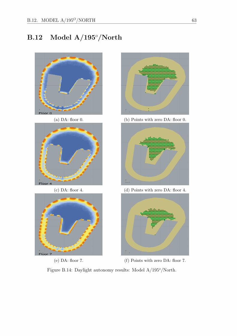
The appendix contains the results of the daylight autonomy for both model B (with-out the daylight from atrium) and model A (with daylight from atrium) at six ori-entations. A coloring scheme from blue to red was used to represent the daylightautonomy values. Blue corresponds to 0 % while red corresponds to 100 % daylightautonomy. The green points seen in the figures on the right corresponds to thesensor points which receive 0 % DA.

50

51

B.0.1 Model images in Rhinoceros

Figure B.1: Building without atrium roof and interior glazing: model B.

Figure B.2: Building with atrium roof and interior glazing: model A.

52 B.1. MODEL B/0O/SOUTH-SOUTHWEST

B.1 Model B/0o/South-southwest

(a) DA: floor 0. (b) Points with zero DA: floor 0.

(c) DA: floor 4. (d) Points with zero DA: floor 4.

(e) DA on floor 7. (f) Points with DA=0: floor 7.

Figure B.3: Daylight autonomy results: Model B/0o/South-southwest.

B.2. MODEL A/0O/SOUTH-SOUTHWEST 53

B.2 Model A/0o/South-southwest


(c) DA: floor 4. (d) Points with DA=0: floor 4.

(e) DA: floor 7. (f) Points with zero DA: floor 7.

Figure B.4: Daylight autonomy results: Model A/0o/South-southwest.

54 B.3. MODEL B/15O/SOUTH

B.3 Model B/15o/South




Figure B.5: Daylight autonomy results: Model B/15o/South.

B.4. MODEL A/15O/SOUTH 55

B.4 Model A/15o/South




Figure B.6: Daylight autonomy results: Model A/15o/South.

56 B.5. MODEL B/60O/SOUTH-EAST

B.5 Model B/60o/South-east


(c) DA on floor 4. (d) Points with zero DA: floor 4.


Figure B.7: Daylight autonomy results: Model B/60o/South-east.

B.6. MODEL A/60O/SOUTH-EAST 57

B.6 Model A/60o/South-east




Figure B.8: Daylight autonomy results: Model A/60o/South-east.

58 B.7. MODEL B/80O/EAST-SOUTHEAST

B.7 Model B/80o/East-southeast




Figure B.9: Daylight autonomy results: Model B/80o/East-southeast.

B.8. MODEL A/80O/EAST-SOUTHEAST 59

B.8 Model A/80o/East-southeast




Figure B.10: Daylight autonomy results: Model A/80o/East-southeast.

60 B.9. MODEL B/105O/EAST

B.9 Model B/105o/East




Figure B.11: Daylight autonomy results: Model B/105o/E.

B.10. MODEL A/105O/EAST 61

B.10 Model A/105o/East




Figure B.12: Daylight autonomy results: Model A/105o/East.

62 B.11. MODEL B/195O/NORTH

B.11 Model B/195o/North

(a) DA on floor 0. (b) Points with zero DA: floor 0.



Figure B.13: Daylight autonomy results: Model B/195o/North.

B.12. MODEL A/195O/NORTH 63

B.12 Model A/195o/North




Figure B.14: Daylight autonomy results: Model A/195o/North.

Appendix C: Cooling loads results

The appendix contains the two models that were simplified before the cooling loadsimulation were performed. The temperatures in the atrium zones are also includedbefore and after the atrium roof glazing was introduced.

64

65

C.0.1 Model Images in IDA ICE

Figure C.1: Building model without atrium glazing as seen in IDA ICE: model B.

Figure C.2: Building model with atrium roof glazing as seen in IDA ICE: model A.

66

C.0.2 Temperatures in the atrium zone

Figure C.3: Temperatures in the atrium zone: model B.

Figure C.4: Temperatures in the atrium zone: model A.

Bibliography

[1] AIA California Council. (2007). Integrated project delivery; a working defini-tion., [Online]. Available: http://aiacc.org/wp-content/uploads/2010/07/A-Working-Definition-V2-final.pdf.

[2] U. T. Aksoy and M. Inalli, “Impacts of some building passive design parame-ters on heating demand for a cold region,” Building and Environment, vol. 41,no. 12, 1742–1754, 2006. doi: 10.1016/j.buildenv.2005.07.011.

[3] G. Ander. (Sep. 15, 2016). Daylighting, [Online]. Available: http://www.

wbdg.org/resources/daylighting.

[4] S. Attia, E. Gratia, A. D. Herde, and J. L. Hensen, “Simulation-based deci-sion support tool for early stages of zero-energy building design,” Energy andBuildings, vol. 49, 2–15, 2012. doi: 10.1016/j.enbuild.2012.01.028.

[5] “CIE general sky standard defining luminance distributions,” Institute of Con-struction and Architecture, Slovak Academy of Sciences, Technical report,2001.

[6] Efficient windows collaborative. (Oct. 3, 2017). Measuring performance: Solarheat gain coefficient (shgc), [Online]. Available: http://www.efficientwindows.org/shgc.php.

[7] B. B. Ekici and U. T. Aksoy, “Prediction of building energy needs in earlystage of design by using anfis,” Expert Systems with Applications, vol. 38, no.5, 5352–5358, 2011. doi: 10.1016/j.eswa.2010.10.021.

[8] A. Elasfouri, R Maraqa, and R Tabbalat, “Shading control by neighbouringbuildings: Application to buildings in amman, jordan,” International Journalof Refrigeration, vol. 14, no. 2, 112–116, 1991. doi: 10.1016/0140-7007(91)90083-s.

[9] EQUA Simulation AB. (Oct. 3, 2017). Software info, [Online]. Available: http://www.equa.se/en/about-us/history.

[10] Ergonomics of the thermal environment- analytical determination and inter-pretation of thermal comfort using calculation of the pmv and ppd indices andlocal thermal comfort criteria, ISO 7730:2005, 2005.

[11] Orn Erlendsson, “Daylight optimization: A parametric study of atrium de-sign,” Master’s thesis, KTH Royal Institute of Technology, Jul. 2014.

[12] G. Florides, S. Tassou, S. Kalogirou, and L. Wrobel, “Measures used to lowerbuilding energy consumption and their cost effectiveness,” Applied Energy,vol. 73, no. 3-4, 299–328, 2002. doi: 10.1016/s0306-2619(02)00119-8.

67

68 BIBLIOGRAPHY

[13] Grasshopper 3D. (Oct. 3, 2017). Grasshopper - algorithmic modeling for rhino,[Online]. Available: http://www.grasshopper3d.com.

[14] greenTEG AG. (Oct. 3, 2017). U-value, [Online]. Available: https://www.greenteg.com/U-Value/.

[15] R. Gupta and R. V. .Ralegaonkar, “Estimation of beam radiation for optimalorientation and shape decision of buildings in india,” Architectural Journal ofInstitution of Engineers India, vol. 85, 27–32, 2004.

[16] J. S. Hygh, J. F. DeCarolis, D. B. Hill, and S. R. Ranjithan, “Multivariateregression as an energy assessment tool in early building design,” Building andEnvironment, vol. 57, no. Supplement C, pp. 165 –175, 2012, issn: 0360-1323.doi: https://doi.org/10.1016/j.buildenv.2012.04.021.

[17] R. Johnson, D. Arasteh, D. Connell, and S. Selkowitz, “Effect of daylightingstrategies on building cooling loads and overall energy performance,” in. Jan.1986.

[18] J. Kanters and M. Horvat, “The design process known as idp: A discussion,”Energy Procedia, vol. 30, 1153–1162, 2012. doi: 10.1016/j.egypro.2012.11.128.

[19] J. F. Kreider, P. Curtiss, and A. Rabl, Heating and cooling of buildings: Designfor efficiency, revised second edition. CRC Press/Taylor & Francis, 2009.

[20] Light and lighting– lighting of work places– part 1: Indoor work places, SS-EN12464-1, 2003.

[21] T. Mingfang, “Solar control for buildings,” Building and Environment, vol. 37,no. 7, 659–664, 2002. doi: 10.1016/s0360-1323(01)00063-4.

[22] G. Mischler. (Oct. 3, 2017). Lighting design glossary, [Online]. Available: http://www.schorsch.com/en/kbase/glossary/luminance.html.

[23] NSG Group. (Oct. 3, 2017). Pilkington sun cool range, [Online]. Available:https://www.pilkington.com/en-gb/uk/products/product-categories/

solar-control/pilkington-suncool-range#rangebrochures.

[24] Passive solar handbook volume i, introduction to passive solar concepts. USAir Force. [Online]. Available: http : / / onebuilding . org / historical /

AirForcePassiveSolarHandbook/pshbk_v1.pdf.

[25] R. Perez, R. Seals, and J. Michalsky, “To all-weather model for sky luminancedistribution—preliminary configuration and validation,” Solar Energy, vol. 51,no. 5, p. 423, 1993. doi: 10.1016/0038-092x(93)90157-j.

[26] D. C. F. Reinhart, Tutorial on the use of daysim simulations for sustainabledesign.

[27] Robert McNeel & Associates. (Oct. 3, 2017). Rhinoceros 3d, [Online]. Avail-able: https://www.rhino3d.com/features.

[28] D. Robinson and A. Stone, “Irradiation modelling made simple: The cumula-tive sky approach and its applications.,” in Plea 2004 – The 21st Conferenceon Passive and Low Energy Architecture, Eindhoven., 2004.

BIBLIOGRAPHY 69

[29] M. S. Roudsari. (Oct. 3, 2017). Ladybugtools, [Online]. Available: http://www.grasshopper3d.com/group/ladybug.

[30] S. Sharples and D. Lash, “Daylight in atrium buildings: A critical review,”Architectural Science Review, vol. 50, no. 4, 301–312, Jan. 2007. doi: 10.

3763/asre.2007.5037.

[31] C. B. de Souza, “Contrasting paradigms of design thinking: The building ther-mal simulation tool user vs. the building designer,” Automation in Construc-tion, vol. 22, no. Supplement C, pp. 112 –122, 2012, Planning Future Cities-Selected papers from the 2010 eCAADe Conference, issn: 0926-5805. doi:https://doi.org/10.1016/j.autcon.2011.09.008.

[32] “Sweden green building council. 5.0 health and wellbeing: Daylight,” BREGlobal Ltd., Tech. Rep., 2003, pp. 54–68.

[33] Swedish Energy agency, “Energi i vara lokaler: Resultat fran energimyndighetensstil2-projekt, delrapport fran energimyndighetens projekt forbattrad energistatistik i samhallet,” Tech. Rep., 2010.

[34] W. Wang, H. Rivard, and R. Zmeureanu, “Floor shape optimization for greenbuilding design,” Advanced Engineering Informatics, vol. 20, no. 4, 363–378,2006. doi: 10.1016/j.aei.2006.07.001.

[35] T. Østergard, R. L. Jensen, and S. E. Maagaard, “Building simulations sup-porting decision making in early design – a review,” Renewable and SustainableEnergy Reviews, vol. 61, 187–201, 2016. doi: 10.1016/j.rser.2016.03.045.

TRITA IES 2017:06

www.kth.se

the effect of an atrium and building orientation on the ...1163933/fulltext01.pdf · 3.6 % of...

Documents