the economic origins of the territorial state - … · the economic origins of the territorial...
TRANSCRIPT
The Economic Origins of the Territorial State∗
Scott Abramson†
Princeton UniversityDepartment of Politics
Abstract
This paper challenges the long standing belief that changes in patterns of war and war-makingcaused the emergence of large territorial states. Using new data describing the universe of Eu-ropean states between 1100 and 1790 I find that small political units continued to thrive wellinto the “age of the territorial state,” an era during which some argue changes in the productionof violence led to the dominance of geographically large political units. In contrast, I find evi-dence that variation in patterns of economic development and urban growth caused fragmentedpolitical authority in some places and the construction of geographically large territorial statesin others. Exploiting random climatic variation in the propensity of certain pieces of geographyto support large populations, I show via an instrumental variables approach that the emergenceof towns and cities caused the formation of small and independent states. Last, I explore howchanges in economic forces interacted with patterns of war-making, demonstrating that the effectof urban development was greatest in periods associated with declines in the costs of producinglarge-scale military force.
∗Thanks to The Columbia-Princeton-Yale Historical Political Economy Working Group, Carles Boix, Peter Buis-seret, Ali Cirone, Joanne Gowa, Kosuke Imai, and Kris Ramsay. Thanks to Emily Erickson, Marco Esquandolas,Eric Falcon, and Jennifer Zhao for their research assistance. Please do not cite or circulate†[email protected]
For the nearly forty years since the publication of The Formation of National States in Western
Europe (Tilly 1975) questions of the territorial state’s origin have aroused the interest of scholars
spanning comparative politics, international relations, and historical sociology. Yet despite an
extensive scholarship on the topic, there has been little work aimed at explicitly testing competing
theories of state formation.1 Bringing to bear new data describing the entire universe of European
states I fill this gap by explaining variation in the number and size of states between 1100 and 1790.
In doing so, my results question several commonly held beliefs about the relationship between war-
making and the origins of the territorial state. In contrast to theories that emphasize the role of
war, I provide evidence that changes in urban growth and the revival of commerce caused observed
temporal and spatial variation in the geographic scale of political organization.
The first half of this paper casts doubt on what I call the “bellicist” approach to state formation.
Heavily influenced by the work of Charles Tilly and dating to German sociologists Otto Hintze and
Max Weber, this line of scholarship attributes the development of the state to changes in patterns
of war and war-making (Hintze 1906; 1975, Weber 1968, Tilly 1975; 1985; 1990, Downing 1992,
Ertman 1997). In these theories “war made states” through a Darwinian process. Large states
could easily raise the manpower and finance required to field the increasingly large standing armies
and increasingly dear technologies of coercion necessary to survive an era of endemic warfare.
Technological shocks to the production of violence requiring increasing numbers of soldiers and
more expensive armaments selected states most capable of adapting to these changes (Roberts 1956,
Parker 1976; 1996, Black 1991, Rogers 1995). Though a number of possible military innovations
are identified, according to this logic the most fit states were those that maintained an advantage in
the form of substantial populations, larger tax bases, and greater access to natural resources (Bean
1973, Finer 1975, McNeill 1984, Tilly 1975; 1985; 1990). Because of these endowments bellicists
argue large states were more capable than their smaller counterparts of meeting the demands of
war and, therefore, were more likely to survive.
1However, several attempts have been made using agent based approaches to examine theories of state formation.For two examples, see Cederman (1997) and Boix, Codenotti and Resta (2011).
1
After introducing a new dataset encompassing the entire universe of European states between
1100 and 1790, I show that several key empirical predictions of war making theories are not borne
out. Namely, I demonstrate that the military revolution, a sequence of dramatic changes to the
production of violence, did not significantly alter the number or typical size of states. In contrast
to the predictions of these bellicist theories, the typical state declined in size and the number of
independent states remained roughly constant during the period associated with these large scale
changes. Moreover, I show that the relationship between geographic scale and survival probability
is the opposite of what war-making theories predict. Specifically, over this span small states were
more likely to survive than their larger counterparts and this relationship was invariant across
time. In other words, rather than being “an age of the territorial state (De Lagarde 1937),” the
period between 1500 and 1800 was one in which small political communities not only persisted but
remained the typical form of political organization.
The second half of this paper provides evidence in favor of the set of what I call “economic”
theories. This scholarship reemerged with the work of Hendrik Spruyt (Spruyt 1994a;b) and builds
upon the political sociology of Stein Rokkan and economic history of Henri Pirenne in viewing the
development of the territorial state in some places (and its absence in others) as the consequence
of variation in the dominant social coalitions that formed from changing patterns of trade and
economic development (Eisenstadt and Rokkan 1973, Rokkan 1975; 1980, Rokkan and Urwin 1982,
North and Thomas 1973, Anderson 1974). Broadly, these theories find that economic changes
which empowered new social groups relative to existing actors can best explain observed patterns
of European state formation. The re-emergence of the Eastern trade and the revival of urban life
during the last half of the tenth century created in some places new commercial classes (Pirenne
and Clegg 1937, Pirenne 1969, Lopez 1976, Cipolla 1994). Where towns formed and burghers could
bargain for or force their rights upon princes and kings, smaller and more numerous political units
came into existence. Common to these accounts is the idea that variation in the economic resources
available to groups explain the type and size of state capable of existing. Indeed, recent work has
shown that geographically small and urban city-states could far easier and earlier construct financial
instruments necessary to purchase the means of defense required to survive interstate competition
2

(Stasavage 2011a;b).
Since the relationship between patterns of state formation and urban growth is likely affected by
unobservable confounders and, moreover, because the direction of causality runs in both directions,
I take an instrumental variables approach to identify the effect of changes in patterns of urban
development on the size and number of states within some defined geography. To show that
political fragmentation was caused by the uneven re-emergence of urban life I exploit random
climatic variation in propensity of some pieces of geography to sustain large populations. Treating
the optimal growing temperature for cereals like wheat as an instrument for the development of
towns and cities, I show that variation in urban growth caused political fragmentation. Where
commerce and urban life reclaimed a foothold, where cities re-emerged from the Dark-Age nadir,
small independent political communities formed. In those places where cities and urban life did not
emerge, large territorial states took shape.
Last, I explore how the mechanisms of economic and war-making theories might be reconciled.
To do this, I show that the effect of urban growth was greatest in periods matched by a concurrent
decline in the costs of producing large scale military force, suggesting an interaction between the
constraints of war and changes in patterns of economic development. In other words, when the
costs of war were low, new social groups created by changing patterns of trade and urban growth
were most capable of claiming and defending independence. More concretely, the period of the
commercial revolution, an era during which there was a sharp increase in the number of independent
states, coincided with the decline in the military dominance of expensive shock calvary and the rise
of armies consisting of comparatively inexpensive infantry armed with pike or bow. In this era, I
show that the effect of urban growth was greatest.
1 What States Are (And Aren’t)
Before any analysis can be conducted, data describing the outcome of interest must be system-
atically collected and defined. To do this in a theoretically satisfying manner it is crucial for my
object of inquiry, the state, to be clearly defined and carefully operationalized. This section first
defines a minimalist Weberian definition of the state. Then, I outline three observable criteria that
3

allow for the systematic and replicable coding of political units as states or not. Next, I argue that
this way of understanding statehood is both reasonable from a historical standpoint and, moreover,
captures the crucial distinction others have highlighted between alternative institutional forms like
the Holy Roman Empire, leagues of city-states, and territorial states.
1.1 A Definition of the State
As a start, I turn to Weber’s treatment of states as political communities that “(successfully)
claim a monopoly on the legitimate use of physical force within a given territory (Weber 1972).”
However, to reflect empirically observable phenomena rather than a non-existent ideal type I alter
this definition, defining states as the organizations that maintain a quasi-monopoly of violence over
a fixed territory. That is, states are the organizations that have a clear preponderance of the
coercive means over some geographically defined unit.
To systematically measure this quasi-monopoly of coercion I provide three necessary observable
criteria to distinguish states from non-states.
1. Direct Military Occupation
If a political unit is militarily occupied by a foreign power, according to my coding scheme it
ceases to exist as an independent state. Similarly, if a political unit successfully conquers a
piece of territory, this newly occupied territory is treated as a part of the conquering state.
For example, when the Ezzelino or Pallavicini families were able to effectively wield military
control over several Italian city-states I code the amalgamation of these units as a single
state. Analogously, when military orders like the Teutonic Knights or the Knights Hospitaller
conquered well defined territories these new units are coded as independent states. Similarly,
when the Castilian-Aragonese state drove the Moors from Grenada, the Emirate of Grenada
ceases to be coded as an independent state and its territory gets coded as part of Castile.
2. The Capacity To Tax
Expropriative power, the ability to take from another that which she owns, is the coercive
authority most associated with statehood. Formal expositions of states as wealth maximizing
4
actors, as “stationary bandits” or organized criminal organizations, underscore this crucial
aspect of state violence: states“steal” from those they govern. Moreover, the ability to extract
is the key feature of state power driving several recent and influential theories of political
transitions (Boix 2003, Acemoglu and Robinson 2006). In these theories it is precisely the
ability of the state to extract that actors - economic classes in these models - enter into conflict
to control. As such, I take the capacity to tax as evidence of the state’s quasi-monopoly of
coercion. So, for example, when Worms (1184) or Lubeck (1226) demonstrably gained rights
to collect taxes and tolls within their boundaries I code them as independent states.
3. A Common Executive
Recognizing that many states during the time period studied were “composite” entities, com-
posed of political units which maintained semi-independent bureaucracies, parliaments, and
other separate political institutions (Nexon 2011), I treat those sharing a common executive
as a single state. Coding states this way treats the holdings of Imperial families as a common
state rather than distinct units. So, for example, all of the territory held by the head of the
Wittelsbach family - at various points including the Counties of Holland, Hainaut and Zee-
land, as well as the Duchies of Julich and Berg - all get coded as a single state. However, as
the family split territory amongst its various component branches - first between the Bavarian
and Palatinate and then the numerous further divisions - each is treated as a distinct state.
However, when, as in 1777 the Bavarian line died out and merged with the Palatinate branch
they again get treated as a single state.
1.2 Relation To Other Definitions of the State
The definition of states as quasi-monopolists of violence recognizes the fact that political commu-
nities that reasonable coders would identify as states existed before juridical notions of sovereignty.
This is not a claim that juridical statehood is unimportant for the study of politics but, rather, that
such a coding scheme would fail to capture political organizations like France, Venice and England
let alone older polities like the Roman or the Han Empires that existed as coercion monopolizing
5

entities long before 1648 or 1555.2 In the words of historian H. J. M. Claessen, we have no reason
to consider “the realm of the Aztecs, the Mongol Empire,...or the late Roman empire qua political
structure as qualitatively different from, say, France, Spain or England in the fifteenth century.
They were all states, varying from early to mature (quoted in Skalnık 1989 p. ix).”
Moreover, because this coding scheme treats the de facto distribution of power as central in
determining which units get coded as states, I treat as distinct political units some states that more
traditional historiography might consider unified. For example, when Boleslaw III of Poland divided
his Kingdom between his sons creating the Masovian, Seniorate, and Sandomierz provinces along
with Greater Poland, my coding scheme treats each as distinct units. Similarly feudal territories like
Toulouse, Provence, or Brittany, which although seigniorial dependants of the French King get coded
as independent until they are integrated into France proper. Likewise, Imperial city states, prince-
bishoprics, free-cities, and imperial abbeys that effectively demonstrate independence as outlined
above get coded as independent units. So, for example, when Fredrick Barabarossa attempted
to assert imperial rule in Lombardy, the various units that composed the Lombard League and
successfully resisted begin to be coded as independent.
With this minimalist notion of statehood I am able to account for institutional configurations
that others treat as distinct from territorial or “national” states. Without rejecting the notion
that political entities like the Holy Roman Empire or the Swabian and Hanseatic leagues were
unique constellations of political institutions we can consider, based upon my scheme, many of
their constituent units as states while still capturing the relevant differences drawn by the liter-
ature between these alternatives and territorial states. They, unlike territorial states, preserved
fragmented political authority.
Consider the Holy Roman Empire. Whether or not it represents a true alternative to the
state, using my coding scheme, I arrive at a conclusion similar to those who, like Spruyt (1994a;b),
view the Empire as a fundamentally unique institutional form. That is, from either perspective
it is apparent that the Holy Roman Empire was marked by substantial fragmentation of political
authority. Indeed, by the end of the thirteenth century an increasing number of units within the
2See Krasner (1999) for a more complete discussion of internal control, external recognition, and Westphaliansovereignty as useful analytic tools
6
Empire acquired de facto independence from Imperial rule. The extent of this was such that even
petty magnates who previously swore“fealty to only God and Emperor eschewed themselves equally
of both powers” and maintained “full jurisdiction... rights of legislation, privileges of coining money,
levying tolls and (collecting) taxes (Bryce 1920; ch. xiv).” They were, by my definition, independent
states. Indeed, “along the Rhine even the Lord of a single tower was often almost an independent
prince (ibid).”
The same is true for leagues of city states. Although leagues like the Hansa were far more
than a loosely bound affiliations of towns centered around the regulation of trade, when considered
in light of my coding scheme they do not represent an alternative to the state. Consider the
difficulties leagues faced at creating compliance. Leagues facilitated cooperation among members
largely through reputational mechanisms (Ewert and Selzer 2006, Greif, Milgrom and Weingast
1994). With respect to generating revenue, like modern international institutions, they faced great
difficulty in directly taxing their members. Instead they relied upon the voluntary compliance of
individual member cities to obtain revenue. Typical of these organizations, lacking a third party
enforcement mechanism the Hansa could at most expel member cities who failed to comply with
calls for revenue (Fink 2011).
The absence of third party enforcement is perhaps best evidenced in leagues’ conduct of military
affairs. The Hansa and other leagues were certainly capable of projecting military force, fielding
armies able to combat large territorial states like Sweden, England, Denmark, and Holland. For
example, at the height of its powers the Swabian league could support armies rivaling those of any
major power, in 1385 raising an army of more than 12,000 infantrymen and 1,200 calvary (Laffan
1957). But the ability to field large armies belied their true capacity to project force. When,
for example, the Hansa waged war against the Danish Crown in 1360 it could not compel all of
its member states to participate in the conflict (Dollinger 1970; p. 70). Similarly, it was in part
because the consent of the forty-odd commissioners (representatives of the individual cities) was
necessary to execute tactical maneuvers that Swabian league was defeated at Doffingen in 1388;
coordination on the battlefield was made so difficult that the allied lords the league opposed were
able to emerge victorious despite their numerical inferiority (Zimmermann 2009).
7

In other words, although leagues were certainly institutional responses to changing patterns of
war and trade, they were organizations comprised of units I call states and not a fundamentally
distinct alternative. Still, perfectly in line with other interpretations, leagues were institutions that
by providing quasi-public or club goods like collective security or enlarged markets for traded goods
allowed fragmented political authority to persist, an outcome captured in my operationalization.
1.3 Constructing the Data
Following this coding scheme the data are constructed by manually geo-referencing several sets of
historical maps. Two of the main sources from which the base GIS boundaries are constructed
are the Centennia Historical Atlas (Reed 2008) and the Euratlas (Nussli 2010) Digital Atlas. The
Nussli data are measured in 100 year panels whereas the Reed atlas utilizes a much more high
frequency approach, recording observations in tenths of years. I use the boundaries as defined by
both datasets aligning them at every hundred year mark based upon the coding scheme defined
above. The Nussli data matches the Reed data nearly perfectly at these points. Where there are
discrepancies it is usually because the Nussli dataset takes observations from a window surrounding
each panel and not a snapshot exactly at the one-hundred year point. Because the Reed data
is not geo-referenced I construct shape files that are compatible with GIS analysis by manually
constructing the boundaries from re-projected images provided by the atlas and then referencing
each observation using the European Albers Equal-Area projection system.
The Nussli data have been used in several recent publications and are considered highly accurate
(Stasavage 2011a;b, Blaydes and Chaney 2012). Nevertheless, even after combining the data from
these digital sources there are still a number of imperfections; units I code as independent states
are absent from the reconstructed shape files. These tend to be small independent principalities,
ecclesiastical units, and city-states that were not picked up by the historical geographers who created
the digital reproductions from which my maps are constructed. In order to rectify these flaws and
prevent the ensuing selection problems that would plague the subsequent statistical analysis, I turn
to a number of historical and contemporary primary source maps to create high frequency boundary
changes for these missing units.
8

This combination of secondary and primary cartographic sources allows me to project the bound-
aries for all political units that meet the coding criteria. Using known pieces of physical geography,
known political boundaries, and the location of cities and towns to properly reference these maps,
I create shape files that, with a high degree of accuracy, reflect the geographic scale of each unit.
For each unit I track the history of their boundary changes - expansions and contractions - and
adjust the shape-files accordingly. In order to provide a more detailed description of the procedure
I walk through the creation of the shape file for part of Nassau between 1159 and 1328.
The town of Nassau dates to at least 915 and was founded by Robert the son of Dudo-Henry of
the House of Laurenburg. The Laurenburgs built Nassau Castle in 1125 and established the County
of Nassau in 1159 - effectively claiming rights of taxation, toll collection, and justice. As such,
Nassau enters the dataset as an independent state as of 1160. The County (later Principality) of
Nassau exists in the digital base maps from this point, giving an accurate measure of its boundaries
and size. However, the digital source maps fail to record the dissolutions and mergers of various
component units of Nassau, of which nearly all meet my coding as independent states. I manually
make these corrections as described below.
For 96 years Nassau existed as a single independent state. Upon the sale of Weilburg to the
Count of Nassau in 1255 the territory was split between the two sons of Henry II with Otto I
receiving the territory north of the river Lahn and his older brother Walram II receiving the rest.
Using this geographic boundary as the dividing line I create the Counties of Nassau-Dillenburg and
Nassau-Weilburg, respectively. Dillenburg remained a single state until Otto’s death in 1303 after
which Nassau-Dillenburg was divided into three units, splitting off Siengen and Hadamar from the
initial unit. The boundaries of these new states are constructed using the boundaries as they exist
on several historical reproductions and one primary source map (Blaeu et al. 1990, Franz 1952,
Hockmann 2005). Using the known latitudes and longitudes of the cities of Siengen and Hadamar I
then can reference the projected images from the historical reproductions using points representing
the locations of these cities. From here, using these points and the boundaries of pre-existing
Nassau-Dillenburg we can create the boundaries and subsequent shape-files for each of these new
units. These three states remained independent until Siengen conquered Dillenburg in 1328 and
9
then Hadamar in 1394.
2 The Military Revolution and The European System of States
In this section I first outline three main empirical predictions made by bellicist theories. Then, I
provide a series of statistical tests showing that the predictions of bellicist theories do not match
the empirical record. Moreover I suggest that these seemingly unwarranted predictions arose from
a literature that has almost exclusively relied upon the historical experiences of extremely large
units to make inferences about general patterns of state formation.
2.1 Predictions of War Making Theories
The general thrust of war-making theories of state formation can be summarized by the dictum,
made famous by Tilly, that “war made states” (Tilly 1985). Indeed, a great deal of wide ranging
historical evidence supports the claim that changes in the patterns of war caused the centralization,
bureaucratization, and rationalization of many activities thought to typify modern statehood. Much
of this literature either directly or indirectly asserts that the pressures of endemic war brought on
by or, in turn, causing changes in the production of violence led to the creation of large states.
Specifically, these changes are described as an early-modern “military revolution,” a notion
first promulgated by Roberts (1956) who viewed changes in infantry tactics devised in the mid
sixteenth century by Maurice of Orange and Gustavus Adolphus as fundamentally altering the
manner in which armies were trained, raised, and paid for. Others view alternative technological
and tactical changes as having marked the sea change between premodern and modern ways of
waging war. Parker (1976; 1996), and McNeill (1984) for example, see as crucial the late-fifteenth
century development of siege artillery, a technological innovation that engendered an even more
costly defensive response, the trace italliene.3
These accounts are not exhaustive. For example, Black (1991), places a greater significance on
3Bean (1973) similarly judges the development of powerful artillery as the crucial technological change and isexplicitly economic in linking the adoption of the cannon to the rise of large territorial states. In his logic, theinnovation of these technologies drove up the fixed costs of war, making local political rule untenable, leading togeographically large states
10
developments that took place between 1660 and 1710, namely, the invention of the flintlock musket.
Rogers (1995), on the other hand dates an almost continuous series of military innovations to the
beginning of the Hundred Years War. Regardless, whether or not the exact timing of the military
revolution is clearly defined, a recurrent theme in the study of early-modern military history is that
a fundamental change in the production of force took place sometime between the mid fifteenth
and the end of the eighteenth centuries.
Social scientists use these historical accounts to build theories of the modern state’s origins,
arguing that a causal relationship exists between military innovation and the rise of geographically
large, territorial states (Tilly 1975; 1985; 1990, Downing 1992, Ertman 1997). Common to them is
the idea that changes in the costs of war selected those states that could pay them. In the canonical
iteration of these theories, the states most fit for survival were those at the intersection of “capital”
and “coercion” (Tilly 1990). These were large states with both sizable populations necessary to
provide the manpower for large standing armies and access to the finance necessary to fund them.
2.2 The Number and Size of States Across Time
With a simple description of the data two trends emerge. First, I show that during the period
associated with the military revolution the typical state declined in size. Second, over the same
period, I find that the number of states remained roughly constant.
2.2.1 The Declining Trend in State Size
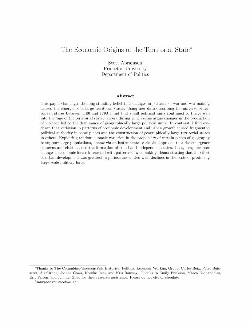
The top panel of Figure 1 plots the trend in state size across time measured in square kilometers.
If one were to only consider the mean, it appears that the bellicist hypothesis matches the general
trend; between 1400 and 1790 the average size of states more than doubled from approximately
33,000 to 71,000 square kilometers. Although a proponent of the military revolution might view this
as confirmation, in the presence of extreme values the mean is a poor indicator of central tendency.
This point is made apparent not only by the large spread between the median of state size and
its mean but by the relationship between the mean and the third quartile of the distribution. For
nearly all of the period for which we have data, the size of the state at the seventy-fifth percentile
11

was less than the mean size.
The reason for this is clear. There are several extremely large states distorting what we might
otherwise view as typical. That is, the distribution of the untransformed data is heavily skewed,
with far more large states relative to what one would expect if size of states took a more symmetric
distribution. An oft used and simple corrective to this type of problem is to log-transform the data
which allows for better descriptive inference about the trend in state size for the typical state.4.
In appendix I show that the log-transformed data are statistically indistinguishable from a normal
distribution.
Although a naive interpretation of the untransformed mean trend would indicate a revolution
in state size coinciding with known changes in military technology, once we transform the data this
upward trend disappears. Rather, the typical state between 1100 and 1790 declined in size. The
lower panel of Figure 1 indicates that both the mean and median state size are declining over time
and in near perfect tandem.5 The decline in both measures is substantial; the mean and median
logged state size decreasing between 1100 and 1790 from 9.03 to 6.32 and 9.62 to 5.67, respectively.
Re-transforming these results gives declines of 7,818 and 14,816 square kilometres from initial values
of 8,372 and 15,106. By these measures the “typical” state, though quite small in 1100, became
even smaller over time, contradicting the theoretical prediction made by war making theories of
state formation.
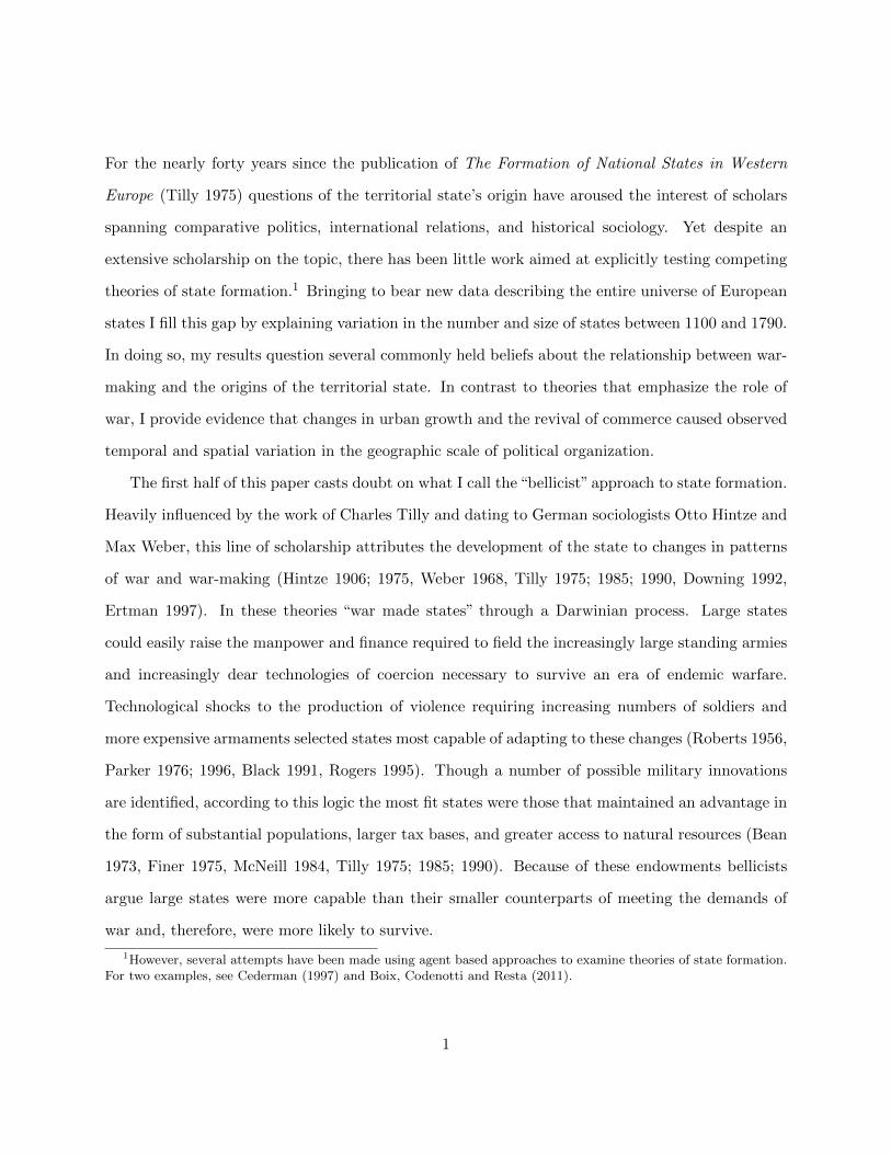
2.2.2 The Trend in the Number of States
A related claim made by proponents of bellecist theories is that number of states capable of sustain-
ing themselves in interstate competition declined during periods associated with large-scale changes
in the production of military violence. However, as with the trend in state size I find no evidence of
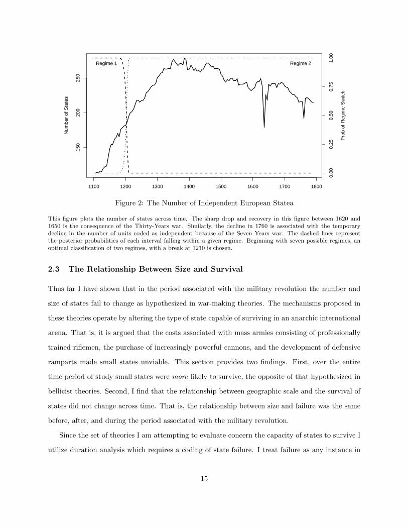
a dramatic reduction in the number of states during the era associated with these changes. Figure
2 shows that instead of declining over time, the number of independent units increased, expanding
4Using a similar approach but examining only 1500 and 1998 Warren, Cederman and Schutte (N.d.) also find thatin both years state sizes are distributed log-normally
5A Engle-Granger two step procedure indicates that the two series are cointegrated. Estimating the followingrelationship Meant - β·Mediant = µt where β is estimated to be 1.04, a Dickey-Fuller test yields a test statistic of-3.69 allowing us with a high degree of confidence to reject the null hypothesis that µt is a non-stationary series.
12

1100 1200 1300 1400 1500 1600 1700 1800
020
000
4000
060
000
Untransformed Data
Year
Squ
are
Kilo
met
ers
75th
25th
Mean
Median
1100 1200 1300 1400 1500 1600 1700 1800
45
67
89
1011
Transformed Data
Year
log(
Squ
are
Kilo
met
ers)
Mean
Median
75th
25th
Figure 1: The Trend in State Size
Both panels present trends in state size across time. The top panel gives the untransformed data and the bottompanel presents the data log-transformed. The red line represents the mean value and the solid black line representsthe median. The dashed lines represent the interquartile range. Note the remarkable symmetry around the medianof the log-transformed data and the absence of such symmetry in the non-transformed data. Similarly note, tandemmovement of the mean and median as one would expect from a normally distributed random variable.
13

rapidly between the twelfth and thirteenth centuries, peaking in the late fourteenth century, and
declining slightly in the period after that.
Did this reduction from a late fourteenth century peak constitute a radical shift in the number
of states within the European system? To better examine this question, I adopt the method
proposed by Park (2010) to identify structural breaks in count processes like the number of states.
This method classifies the set of time periods where the number of states can be described by a
common data generating process. Moreover, it determines when changes in this process occur.6
Implementing this procedure results in the choice of a single change-point dated at 1210. Figure
2 plots on the right hand axis the posterior probability of a change in regime, demonstrating the
break at 1210. The mean of the first period is estimated to be 130.1 with a 95% credibility interval
of [124.3, 135.7] and the mean for the second period is estimated to be 227.8 with a 95% credibility
interval of [225.1, 230.7].
From this, two substantive conclusions can be drawn. First, the break identified in the early
thirteenth century precedes by several centuries the events bellecist theories argue caused a fun-
damental change in the number of states. Second, the change proposed by this group does not
materialize; the second regime identified by the model, that containing the entire period associated
with the military revolution, has on average a greater number of states. In other words, during
the period in which bellicist theories predict a decline in the number of states we see no dramatic
change in the number of states.7
To summarize, although the bellicist literature describes a military revolution taking place
at some point between 1450 and 1700, its predicted consequences fail to materialize when the
data is examined systematically. During the period associated with large systemic changes in the
production of violence two facts emerge: 1.) The typical state declined in size and 2.) The number
of independent states saw no radical decline, though decreased slightly.
6A technical description of the method and estimation are included in the appendix.7Stasavage (2012) looking at a subset of 168 city-states shows a similar pattern.
14
1100 1200 1300 1400 1500 1600 1700 1800
150
200
250
Num
ber
of S
tate
s
0.00
0.25
0.50
0.75
1.00
Pro
b of
Reg
ime
Sw
itch
Regime 1 Regime 2
Figure 2: The Number of Independent European Statea
This figure plots the number of states across time. The sharp drop and recovery in this figure between 1620 and1650 is the consequence of the Thirty-Years war. Similarly, the decline in 1760 is associated with the temporarydecline in the number of units coded as independent because of the Seven Years war. The dashed lines representthe posterior probabilities of each interval falling within a given regime. Beginning with seven possible regimes, anoptimal classification of two regimes, with a break at 1210 is chosen.
2.3 The Relationship Between Size and Survival
Thus far I have shown that in the period associated with the military revolution the number and
size of states fail to change as hypothesized in war-making theories. The mechanisms proposed in
these theories operate by altering the type of state capable of surviving in an anarchic international
arena. That is, it is argued that the costs associated with mass armies consisting of professionally
trained riflemen, the purchase of increasingly powerful cannons, and the development of defensive
ramparts made small states unviable. This section provides two findings. First, over the entire
time period of study small states were more likely to survive, the opposite of that hypothesized in
bellicist theories. Second, I find that the relationship between geographic scale and the survival of
states did not change across time. That is, the relationship between size and failure was the same
before, after, and during the period associated with the military revolution.
Since the set of theories I am attempting to evaluate concern the capacity of states to survive I
utilize duration analysis which requires a coding of state failure. I treat failure as any instance in
15

which an existing state ceases to appear as an independent political unit according to my coding
scheme. Thus, if a state is conquered it is treated as failing. If two states merge I treat the new
state as either a new unit (and the pre-existing states as being censored) or if it is clear that
one subsumed the other I treat the subsumed state as having failed. In the few cases where this
is ambiguous I alternate codings and re-estimate the model with each possible alternative. The
treatment of these ambiguous cases does not substantively change the results.
The relationship between the hazard rate (the instantaneous rate of failure) and the geographic
size of states is estimated via a mixed effects Cox proportional hazards model of the basic form
λi(t) = λ0(t)× exp(δp · ln(Sizeit) + εi + ηv)
Time is described in three ways. First, t, indexes the time in years since a state came into existence.
Second, v indexes chronological time, e.g. 1445 or 1750 and third, p captures a multi-year period
in chronological time, e.g. 1450 to 1500.
The baseline hazard rate is captured by λ0(t). The relationship between size and the hazard rate
is captured by the set of parameters δp = µ + γp where it is assumes that γp - the period varying
effect - is distributed N ∼ (0, σ2γ) and where µ, captures the time invariant, mean, relationship
between state size and failure. The magnitude of each γp signifies the deviation for each period
p from the time invariant mean effect µ. I present results allowing the effect of state size to vary
by 100 and 50 year intervals, respectively. Since the data includes repeated observations, that is,
because some states fail and then reappear only to fail again, I follow convention and include a unit
specific random “frailty” effect, εi. Similarly following convention, because failure times might be
clustered by chronological time, I include a time random effect, ηv.
First I estimate the model without the time varying component and find that, in contrast to the
conclusions of bellicist theories, there is a robust negative relationship between the probability of
survival and the size of states. That is, I find that geographically large states are more likely to fail
than their smaller counterparts. I then estimate the same model, allowing the effect of size to vary
across period. The magnitude of these effects are roughly uniform across models. Figure 3 plots
these coefficient estimates. In the left panel I plot µ, the parameter capturing the time invariant
16

relationship between size and the hazard rate, which is positive and statistically significant in all
specifications. To gauge the magnitude of this effect, I have plotted in Figure 4 survival curves
from the most conservative model, manipulating state size from the first to the third quartile. A
substantial difference is apparent. For example, having survived up to 100 years the probability of
surviving in the next period is roughly one third less for the state at the seventy-fifth percentile of
state size than the state at the twenty-fifth.
In order to examine the hypothesis that the relationship between size and failure changed during
the period associated with the military revolution I compare the time varying effect of size γp across
periods. Since each γp captures the period specific deviation from µ, if γp differs in a statistically
significant way from zero we can say that for period p the relationship between geographic scale
and survival differed from the average effect. Plotted in the right-hand panel of Figure 3 we see
that this is not true for any time period; none of the time varying effects differ in a statistically
significant way from zero and, moreover, I find no statistically significant difference between any
pair of time periods.8
Matching the results from the previous section, I find no evidence in favor of the notion that the
military revolution affected the size of states. The survival probability of small states was greater
than that of large states. Moreover, the data find no evidence of a change in the relationship
between geographic scale and failure during the expected period. Indeed, I find that the positive
relationship between size and the failure rate of states did not change in a statistically significant
way across time.
2.4 Case Selection and War Making Theories
The (mis)use of the untransformed, skewed data, to draw conclusions about broad patterns of state
formation is mirrored in the case selection of historical scholarship relating war to patterns of state
formation. That is, it is the history of these large states that proponents of war-making theories
of the state build upon. For example, Roberts, a historian of Sweden, draws upon the Swedish
experience in the Thirty-Years war to make conclusions about the effects of new infantry tactics
8Table 5 in the appendix presents the differences and measures of uncertainty for each pair of period varyingparameters.
17

Estimate Size
µγ
0.000.050.100.150.200.25
Mod
el 1
Mod
el 2
Mod
el 3
Mod
el 4
Cox
PH
Cox
Mix
ed E
ffect
sTi
me
Var
ying
Slo
pes
Mod
el 3
Estimate Size
γ 1200
γ 1300
γ 1400
γ 1500
γ 1600
γ 1700
γ 1800
-0.100.000.10
Mod
el 4
Tim
e V
aryi
ng P
aram
eter
Estimate Sizeγ 1150γ 1200γ 1250γ 1300γ 1350γ 1400γ 1450γ 1500γ 1550γ 1600γ 1650γ 1700γ 1750γ 1800
-0.100.000.10
Fig
ure
3:
The
left
panel
plo
tsth
epara
met
eres
tim
ate
sof
the
tim
ein
vari
ant
rela
tionsh
ipb
etw
een
size
and
the
haza
rd.
Model
s1.
and
2.
do
not
incl
ude
tim
eva
ryin
ges
tim
ate
sof
this
effec
t.M
odel
2.
isa
standard
Cox
-pro
port
ional
haza
rds
model
and
does
not
incl
ude
any
random
effec
ts.
Model
s3.
and
4.
incl
ude
per
iod
vary
ing
effec
tsof
size
.M
odel
3.
allow
sth
eeff
ect
of
size
tova
ryby
100
yea
rp
erio
ds
and
Model
4.
allow
sth
eeff
ect
of
size
tover
yby
50
yea
rp
erio
ds.
Thes
ep
erio
dva
ryin
geff
ects
,none
of
whic
hare
stati
stic
ally
dis
tinguis
hable
from
zero
,are
plo
tted
inth
eri
ght
panel
.
18

0 100 200 300 400 500 600 700
0.0
0.2
0.4
0.6
0.8
1.0
Time (Years)
Sur
viva
l Cur
ve
75th 25th
Figure 4: The estimated survival curves from Model 2 from a manipulation of logged size acrossits inter-quartile range. The top line represents the survival curve for a state at the 25th percentileof logged state size. The bottom line represents the same value for a state at the 75th percentile.The dashed lines represent 95% confidence intervals for the survival curve.
across Europe. Parker, a scholar of Early Modern Spain draws similar conclusions based upon his
favored case. Indeed, the extreme cases, Russia, the Ottoman Empire, Sweden, Spain, France, and
England are those scholarship has largely drawn upon to make inferences about general patterns
of war and state formation.
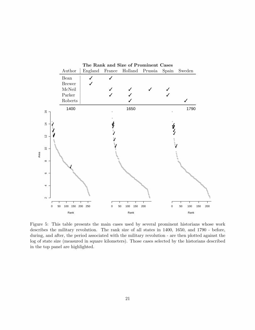
Figure 5 presents the cases that five prominent historians have used to argue in favor of a military
revolution, highlighting both their rank and size relative to the entire distribution of state sizes.
Though not exhaustive, the list is reflective of the general empirical approach this vast historical
literature has taken. The lower panel of Figure 5 describes the entire distribution of state sizes,
plotting the rank of each state against its size in logged square kilometers at three points in time:
1400, 1650, and 1790; right before the military revolution, following the Thirty-Years war, and at
19

the close of this study. We see that when selecting cases historical scholarship emphasizing the role
of war has drawn from, almost exclusively, the extreme end of the distribution of state sizes.
Unlike the historical case studies that emphasize the role of war in determining processes of
state formation, the empirical approach of proponents of economic theories does not exclusively
rely upon the experiences of large outlying states. For example, Spruyt (1994a;b) in highlighting
the experiences of the city-states comprising the Hanseatic League, finds in favor of economic causes.
In taking a more quantitative approach Stasavage (2011a;b) stresses the advantage small states had
in constructing financial instruments necessary to fund defense and therefore survival. Taking
advantage of the full distribution of observed outcomes, in the next section I provide evidence in
favor of economic theories.
3 Commerce and the Origins of the Modern State
The causal link between the revival of commerce and patterns of European state formation has been
drawn by a number of scholars. Despite this, few systematic empirical tests of this relationship
have been undertaken. This section briefly outlines the relevant literature tying the re-emergence
of commerce and urban life to political fragmentation.
In an early incarnation, Stein Rokkan (Eisenstadt and Rokkan 1973, Rokkan 1975; 1980, Rokkan
and Urwin 1982) argued that the existence of a “city belt”9 running through central Europe was
the crucial determinant explaining why the modern territorial state developed in places peripheral
to this productive core. The existence of a large number of prosperous urban centers prevented the
rulers of any one from consolidating rule over the others. In peripheral England and France, for
example, the absence of many urban centers allowed monarchs, by force or diplomacy, to establish
rule over expansive territories.
Spruyt (1994b) views the creation of new social groups as both an outcome of the revival of
commerce and a catalyst for premodern innovation in the organization of the state. In those places
where trade resumed new towns and cities formed as hubs of economic life, allowing a class of
9Rokkan at various times refers to the region I identify as the European core as the “trade belt,”“middle belt,”“city-studded centre,”“city-state Europe,”“heartland,” and “dorsal spine”
20
The Rank and Size of Prominent CasesAuthor England France Holland Prussia Spain Sweden
Bean 3 3
Brewer 3
McNeil 3 3 3 3
Parker 3 3 3
Roberts 3 3
●●●●●
●●●●●●●
●●●●●
●●●●●●
●●●●●●●●
●●●●●●●
●●●●●●●●●●●●
●●●●●●●●●●●●
●●●●●●●●●●
●●●●●●●●●●
●●●●●●●●●●
●●●●●●●
●●●●●●●●●●●
●●●●●●●●●
●●●●●●●●●●●●
●●●●●●●●●●●●●●
●●●●●●●●
●●●●●●●●●●
●●●●●●●●
●●●●●●●●●
●●●●●●●●●●●
●●●●●●
●●●●●●●●●●
●●●●●
●●●●●●
●●●●●●●
●●●●●●●●●
●●●●●●●●
●●●●
●●●
●●
●●●
●
●
Rank
Are
a
24
68
1012
1416
0 50 100 150 200 250
1400
●●●●
●●●●
●●●●●●●●●●●●
●●●●●●●●●●●
●●●●●●●●●●
●●●●●●●●●●●
●●●●●●●●
●●●●●●●●●●●●
●●●●●●●●●●●
●●●●●●●●●●●●●
●●●●●●●●●●●
●●●●●●●●●●●●
●●●●●●●●●●●●●●●
●●●●●●●●●●●●●
●●●●●●●●●
●●●●●●●●●
●●●●●●●●●
●●●●●●●
●●●●●●●●●
●●●●●●●
●●●●●●●●●●●
●●●●●●●●●
●●
●●●●●●●
●●●
●●
●
●
Rank
0 50 100 150 200
1650
●●●●●●●
●●●●
●●●●●●●
●●●●●●●●
●●●●●●●●
●●●●●●●●●●●
●●●●●●●●
●●●●●●●●●●●
●●●●●●●●●●●●
●●●●●●●●●●●●●
●●●●●●●●●●
●●●●●●●●●●
●●●●●●●●●●●
●●●●●●●●●●●●●
●●●●●
●●●●●●●●●
●●●●●●●
●●●●●●●●●
●●●
●●●●●
●●●●●●●●●●
●●●●●●
●●●●
●
●●●
●●●●●
●●●
●
●
●
●
Rank
0 50 100 150 200
1790
Figure 5: This table presents the main cases used by several prominent historians whose workdescribes the military revolution. The rank size of all states in 1400, 1650, and 1790 - before,during, and after, the period associated with the military revolution - are then plotted against thelog of state size (measured in square kilometers). Those cases selected by the historians describedin the top panel are highlighted.
21
burghers to establish effective independence. By virtue of these groups’ economic power, monarchs,
particularly the Holy Roman Emperor, were impeded in their attempts to create geographically
large states and were forced into political bargains accepting the de facto independence of these
states. Moreover, because of their wealth and ability to establish institutions like the Hansa capable
of providing collective security these states could wield sufficient military force to not merely claim
independence but to sustain it over time.
What is common amongst these economic theories is that changes in patterns of economic
activity, principally those associated with changes in commerce and urban life altered the balance of
political power, causing political fragmentation in the urban core of Europe. This section examines
trends in the number and size of states at the regional level, providing evidence that only in the
most productive places in Europe, a central regional band extending, roughly, in an arc from the
Low Countries, through the Rhineland and into Northern Italy, could small political communities
persist. That is, in the places where the “commercial revolution” of the first half of the previous
millennium took hold political fragmentation ensued. However, in less productive regions, in the
absence of dense urban and commerical growth, large territorial states formed.
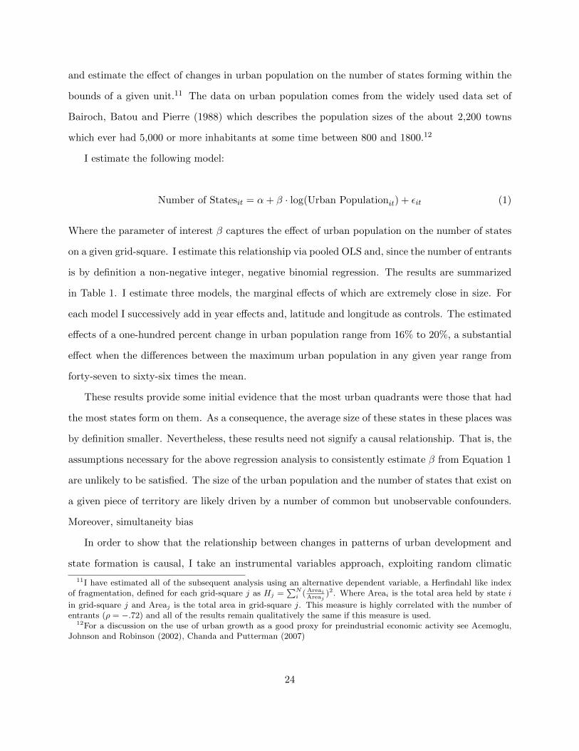
As initial evidence Figure 6 plots both the trend in logged state size and number of states across
time, first dividing the map into two broad regions: the urban European core, the area described
above, and the remainder of the map, what I will call the periphery. In both regions the number
of states is increasing before the early thirteenth century. After this period the upward trend in
the number of states continues in Central Europe whereas in the periphery it plateaus and then
begins to decline in the early fifteenth century. Similarly the average size is initially declining in
both groups. However, in the periphery, beginning in the early sixteenth century, the average size
starts to increase whereas it continues to decline in the center.10
These patterns coincide with the reemergence of trade and a general revival of commercial and
urban life during the first third of the millennium. Like the regional pattern in the number and size
of states these economic trends were not uniform across space but were geographically concentrated
10We can divide the continent into a number of more refined regions, however, the same pattern holds; fragmentationand decline in size concentrated within the productive core and consolidation and increased size following the fifeteenthcentury in all regions in the periphery
22

Number of States
Cou
nt
5010
015
020
0
Core
Periphery
Trend in State Size
Year
Cha
nge
in S
ize
−0.
750.
251.
00
1100 1200 1300 1400 1500 1600 1700 1800
Figure 6: The average size and number of states separating out the urban European from therest of the continent. In both plots the black line represents the core of Europe and the dashedline represents the periphery. The top panel plots against time the number of states in these tworegions. The lower panel plots for each region the difference between the mean of log-transformeddata in a given year and the mean for the entire (regional) series.
in a manner nearly identical to the patterns of state formation described above. The emergence of
towns and cities - a product of the geographically concentrated revival of commerce and economic
development - created groups in these places with the resources necessary to maintain or claim
independence, thereby preventing the consolidation of territorial states.
3.1 Urban Growth and State Formation
This section directly estimates the causal relationship between development and state formation.
As the unit of analysis I employ arbitrarily defined pieces of geography, 10,000 km2 grid squares,
23
and estimate the effect of changes in urban population on the number of states forming within the
bounds of a given unit.11 The data on urban population comes from the widely used data set of
Bairoch, Batou and Pierre (1988) which describes the population sizes of the about 2,200 towns
which ever had 5,000 or more inhabitants at some time between 800 and 1800.12
I estimate the following model:
Number of Statesit = α+ β · log(Urban Populationit) + εit (1)
Where the parameter of interest β captures the effect of urban population on the number of states
on a given grid-square. I estimate this relationship via pooled OLS and, since the number of entrants
is by definition a non-negative integer, negative binomial regression. The results are summarized
in Table 1. I estimate three models, the marginal effects of which are extremely close in size. For
each model I successively add in year effects and, latitude and longitude as controls. The estimated
effects of a one-hundred percent change in urban population range from 16% to 20%, a substantial
effect when the differences between the maximum urban population in any given year range from
forty-seven to sixty-six times the mean.
These results provide some initial evidence that the most urban quadrants were those that had
the most states form on them. As a consequence, the average size of these states in these places was
by definition smaller. Nevertheless, these results need not signify a causal relationship. That is, the
assumptions necessary for the above regression analysis to consistently estimate β from Equation 1
are unlikely to be satisfied. The size of the urban population and the number of states that exist on
a given piece of territory are likely driven by a number of common but unobservable confounders.
Moreover, simultaneity bias
In order to show that the relationship between changes in patterns of urban development and
state formation is causal, I take an instrumental variables approach, exploiting random climatic
11I have estimated all of the subsequent analysis using an alternative dependent variable, a Herfindahl like indexof fragmentation, defined for each grid-square j as Hj =
∑Ni ( Areai
Areaj)2. Where Areai is the total area held by state i
in grid-square j and Areaj is the total area in grid-square j. This measure is highly correlated with the number ofentrants (ρ = −.72) and all of the results remain qualitatively the same if this measure is used.
12For a discussion on the use of urban growth as a good proxy for preindustrial economic activity see Acemoglu,Johnson and Robinson (2002), Chanda and Putterman (2007)
24
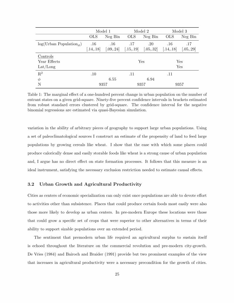
Model 1 Model 2 Model 3
OLS Neg Bin OLS Neg Bin OLS Neg Bin
log(Urban Populationit) .16 .16 .17 .20 .16 .17[.14,.18] [.09,.24] [.15,.19] [.05,.32] [.14,.18] [.05,.29]
ControlsYear Effects Yes YesLat/Long Yes
R2 .10 .11 .11φ 6.55 6.94N 9357 9357 9357
Table 1: The marginal effect of a one-hundred percent change in urban population on the number ofentrant states on a given grid-square. Ninety-five percent confidence intervals in brackets estimatedfrom robust standard errors clustered by grid-square. The confidence interval for the negativebinomial regressions are estimated via quasi-Bayesian simulation.
variation in the ability of arbitrary pieces of geography to support large urban populations. Using
a set of paleoclimatological sources I construct an estimate of the propensity of land to feed large
populations by growing cereals like wheat. I show that the ease with which some places could
produce calorically dense and easily storable foods like wheat is a strong cause of urban population
and, I argue has no direct effect on state formation processes. It follows that this measure is an
ideal instrument, satisfying the necessary exclusion restriction needed to estimate causal effects.
3.2 Urban Growth and Agricultural Productivity
Cities as centers of economic specialization can only exist once populations are able to devote effort
to activities other than subsistence. Places that could produce certain foods most easily were also
those more likely to develop as urban centers. In pre-modern Europe these locations were those
that could grow a specific set of crops that were superior to other alternatives in terms of their
ability to support sizable populations over an extended period.
The sentiment that premodern urban life required an agricultural surplus to sustain itself
is echoed throughout the literature on the commercial revolution and pre-modern city-growth.
De Vries (1984) and Bairoch and Braider (1991) provide but two prominent examples of the view
that increases in agricultural productivity were a necessary precondition for the growth of cities.
25

Nicholas (1997) is rather succinct in describing this logic.
Cities could not develop until the rural economic could feed a large number of people
who, instead of growing their own food, compensated the farmer by reconsigning his
products and later by manufacturing items that the more prosperous peasants desired.
The ‘takeoff’ of the European economy in the central Middle Ages is closely linked to
changes in the rural economy that created an agricultural surplus that could feed large
cities [p. 104]
To identify the causal effect of urban development on state formation in an instrumental vari-
ables framework I exploit random climactic variation in the ability of a given location to produce
key agricultural outputs necessary to support large populations. The natural predisposition for
some places to feed large groups has been directly related to the development of urban life and the
revival of commerce by a number of economic historians. Pirenne (1969), for example, argues that
the location of towns in premodern Europe was a function of natural geography, that “In a more
advanced era, when better methods would permit man to conquer nature and to force his presence
upon her despite handicaps of climate or soil, it would doubtless have been possible to build towns
anywhere the spirit of enterprise and the quest of gain might suggest a site.” This was, however,
not the case. Rather, “...the first commercial groups were formed in neighborhoods which nature
had disposed to become...the focal points of economic circulation.”
I focus on the ability of some places to produce cereals like wheat and barley for two reasons.
First, the European diet of the premodern era was centered around the consumption of complex
carbohydrates derived from cereals. Economic historian Robert Lopez notes that “in the form of
bread, porridge, or mush, cereals were almost everywhere the basis of human alimentation...(Lopez
1976).” Not only were cereals central to diets across European geography but across classes as well
and were integral to the consumption of the aristocracy and peasantry alike although certainly in
unequal proportions (Duby, Clarke and Becker 1974).
Second, the ability to grow cereals has been directly linked to the support of large populations.
Cereals like wheat, unlike other plants, are most capable of feeding large populations with minimal
effort; cereal crops, unlike fruits, pulses, or nuts, are extremely fast growing, high in calories from
26
carbohydrates, and have extremely high yields per hectacre (Diamond 1997). Moreover, unlike
other crops cereals can be stored for long periods of time enabling communities to smooth con-
sumption over extended periods. To summarize, the ability to feed large populations was key to
the development of cities. Since in pre-modern Europe the principle component of diets were cere-
als like wheat, foods that are particularly good at supporting large populations, climatic variation
across time and space in the ability to grow these crops serves as a good encouragement for urban
growth.
The instrument is constructed in two steps:
1. I take spatially referenced temperature data from two paleo-climatological sources, both mea-
sured at half-degree by half-degree latitude/longitude intervals. The first measure from Mann
et al. (2009) records temperature anomalies for the past 1500 years. A temperature anomoly
captures the deviation at each point from the 1961-2000 mean temperature. I then construct
a measure of absolute temperature by adding back the 1961-2000 baseline mean temperature
as calculated from Jones et al. (1999)’s twentieth century data. This yields a half degree
by half degree grid of temperatures for every year over the past 1500 years. Hundred year
averages of these yearly measures are then taken.
2. Next, using tension weighted splines I take these estimates, measured at fixed intervals, and
construct a smoothed measure of temperature for the entire continent. From this continuous
measure the average for each grid-square is taken yielding an estimate of temperature across
our fixed but arbitrary pieces of geography. All of these operations are taken using the
interpolation and zonal averaging tools found in ArcGIS 10.
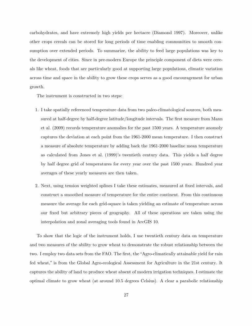
To show that the logic of the instrument holds, I use twentieth century data on temperature
and two measures of the ability to grow wheat to demonstrate the robust relationship between the
two. I employ two data sets from the FAO. The first, the“Agro-climatically attainable yield for rain
fed wheat,” is from the Global Agro-ecological Assessment for Agriculture in the 21st century. It
captures the ability of land to produce wheat absent of modern irrigation techniques. I estimate the
optimal climate to grow wheat (at around 10.5 degrees Celsius). A clear a parabolic relationship
27

●
●
●
●
●
●
●
●
●
●
● ●
●
●
●●
●
●●
●
●
●
●
●
●
●
●●
●●
●
●
●
●
●
●
●
●
●
●
●
●
●
●
●
●
●
●
●
●
●
● ●
●
●●
●
●●
●
●
●
●● ●
●
●
●
●
●
●
●
● ●
●
●
●
●
●●
●
●
●
●
●
●
●
●
●
●●
−5 0 5 10 15 20 25
24
68
1012
14
Mean Temperature (1960−2000)
Agr
icul
tura
l Sui
tabi
lity
Figure 7: The FAO wheat suitability index is plotted on the y-axis against average annual temper-ature on the x-axis. The FAO measure is the “Agro-climatically attainable yield for rain fed wheat”is from the Global Agro-ecological Assessment for Agriculture in the 21st century. It captures theability of land to produce wheat absent of modern irrigation techniques. A clear parabolic rela-tionship with a peak at approximately 10.5 degrees Celsius is observed. The radius of each circleis proportional to the average wheat yield between 1960 and 2000
between temperature and this FAO measure is observed simply by plotting it against average annual
temperature between 1960 and 2000.
Regressing the FAO measure of wheat suitability on the absolute deviation from 10.5 degrees we
see that, indeed there is a negative relationship between the two. The results from this regression
are summarized in first column of Table 2. The effect of a one degree deviation from the optimal
temperature is substantial, decreasing the FAO measure by .61 units. This is a particularly large
effect since the FAO measure is on a fourteen point scale. Moreover, an large amount of the
variation in the FAO wheat suitability measure is explained by deviation from this optimal growing
temperature, the R2 statistic is calculated to be .55. In addition, regressing average annual wheat
yields between 1960 and 1990 on deviation from the optimal growing temperature again shows a
similarly robust relationship. A one degree deviation from the optimal temperature has a large
effect on average annual wheat yields – approximately 1600 hectograms per hectare.
28
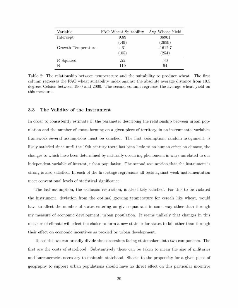
Variable FAO Wheat Suitability Avg Wheat Yield
Intercept 9.89 36901(.49) (2659)
Growth Temperature -.61 -1612.7(.05) (254)
R Squared .55 .30N 119 94
Table 2: The relationship between temperature and the suitability to produce wheat. The firstcolumn regresses the FAO wheat suitability index against the absolute average distance from 10.5degrees Celsius between 1960 and 2000. The second column regresses the average wheat yield onthis measure.
3.3 The Validity of the Instrument
In order to consistently estimate β, the parameter describing the relationship between urban pop-
ulation and the number of states forming on a given piece of territory, in an instrumental variables
framework several assumptions must be satisfied. The first assumption, random assignment, is
likely satisfied since until the 19th century there has been little to no human effect on climate, the
changes to which have been determined by naturally occurring phenomena in ways unrelated to our
independent variable of interest, urban population. The second assumption that the instrument is
strong is also satisfied. In each of the first-stage regressions all tests against weak instrumentation
meet conventional levels of statistical significance.
The last assumption, the exclusion restriction, is also likely satisfied. For this to be violated
the instrument, deviation from the optimal growing temperature for cereals like wheat, would
have to affect the number of states entering on given quadrant in some way other than through
my measure of economic development, urban population. It seems unlikely that changes in this
measure of climate will effect the choice to form a new state or for states to fail other than through
their effect on economic incentives as proxied by urban development.
To see this we can broadly divide the constraints facing statemakers into two components. The
first are the costs of statehood. Substantively these can be taken to mean the size of militaries
and bureaucracies necessary to maintain statehood. Shocks to the propensity for a given piece of
geography to support urban populations should have no direct effect on this particular incentive
29

to form or dissolve as an independent state. The instrument perturbs the major component of the
second constraint, the economic surplus available for latent or existing states to claim, here measured
by urban population. The question then becomes do changes in this measure of temperature affect
economic incentives not captured by changes in urban population?
Here, we must recognize two facts about the preindustrial economy. First is transportation costs
were extremely high such that long distance trade was concentrated in luxury goods (Findlay and
O’Rourke 2007). As such, markets for agricultural products were for much of this period local.13
Second, the market for surplus agricultural product was concentrated in towns and cities. That
is, those who specialized in non-agricultural sectors - located in towns - exchanged their goods for
the surplus agricultural product produced in the hinterland. Because of the limited ability to trade
these goods across extreme distances, changes in the productivity of agriculture affect these local
markets either by shifting labor from the countryside to towns or by allowing a greater number
individuals to specialize in non-agricultural activity, both of which result in a greater number of
people living in towns and cities. Since my measure of urban population includes towns as small
as 1,000 individuals, we should pick up these dynamics.
Moreover, since the changes in optimal growing temperature over a hundred year panel are
extremely slow, the long term tend in which would be very difficult to perceive at any given point
in time in an era before meteorological data was systematically collected. Because of this these
changes would only effect the economic incentive to form states through their long term effects -
the ability to sustain large populations.
13Whyte (1979), for example, argues that in early-modern Scotland there existed a limit of 22 kilometers inlandfrom the coast or major rivers beyond which the cost of overland transport prohibited large-scale trade in grains.Others similarly view the creation of national and international markets for agricultural products like grain as beingrelatively late phenomena. Gras (1915), for example, famously argued that before the seventeenth century Englandconsisted of at least fifteen distinct agricultural markets. Econometric evidence finds support for this claim. ForEngland Bowden (1990) shows a process of declining wheat price differentials between the late fifteenth century andmid eighteenth century. Using a similar methodology, Weir (N.d.) finds that by the mid eighteenth century Franceconsisted of several distinct markets for grain. With perhaps the best sub-national data, Gibson and Smout (2008)similarly show that a national market for oatmeal emerged in Scotland slowly between 1660 and 1780, with much of theconvergence in prices across space occurring after 1750. The evidence concerning international trade in agriculturalproducts is even more stark. In a number of recent econometric studies little or no apparent market integration inthe form of diminished price differentials can be found throughout the early modern age. See, evidence from all ofEurope see Unger (1999), Allen (2001),Ozmucur, Pamuk and Center (2007) ,and Bateman (2011) the latter of whichexploits the most comprehensive dataset on wheat prices in terms of geographic and temporal coverage. Inter-regionalevidence, for example that provided by Allen and Unger (1990) and Unger (1999) arrives at a similar conclusion ofgeographically disjoint markets for grains.
30

Nevertheless, in case the growing climate for wheat has some direct effect on urban population I
attempt to control for alternative channels through which the optimal growing temperature might
effect state formation. I control for the ways in which climate, other than though the deviation
from this optimal temperature for cereals, might effect the number of states on a given square. I
do this in two ways. The first is by controlling for both latitude and longitude. Since climate is
strongly correlated with geographic location, controlling for the position in space should similarly
control for the effects of climate other than through the optimal growing temperature.
By including grid square fixed effects we get similar results. Here identification comes from
within unit variation, deviation from the mean of the unit’s distance from the optimal growth
temperature for cereals. In this sense we are again controlling for long term climatic conditions and
identification is only coming from the random changes from this long-term value. A Hausman test
fails to reject the null hypothesis that the 2SLS fixed effects parameter estimates are different from
the pooled 2SLS estimates, indicating that controlling for latitude and longitude accounts for all
time invariant aspects of climate. Similarly, I estimate the same instrumental variables model in
first differences, where identification is coming exclusively from century-on-century changes in the
propensity to support urban populations. The results are similar though less precisely estimated.
Moreover, although the results are nearly identical, in the first-differenced 2SLS estimates the
instrument fails to meet “rule of thumb” levels of strength (Stock and Yogo 2005).14
3.4 Instrumental Variables Results
The instrumental variables estimates of β, interpreted as the effect of a 100 % change in urban
population on the number of states forming on an arbitrary piece of land, are shown in Table 3.
The effect sizes are rather large, a one hundred percent increase in total urban population on a
given grid-square is expected to increase the number of states locating within that same unit by
14One might worry about violations of exclusion that operate through the spatial correlation of the dependentvariable. That is, the instrument may be correlated across space and consequently its effects on the number of statesin one quadrant might directly effect those in another other. To account for this possibility I have estimated all of the2SLS models in an FGLS framework to account for arbitrary serial correlation across observations. The results remainnearly identical. Additionally, I conduct a Lagrange multiplier test for error dependence in the possible presence ofa missing spatially lagged dependent variable. In the specifications that rely upon within-unit variation I find noevidence of a missing spatial lag. However, in the pooled estimates I cannot reject the possibility.
31

Instru
menta
lVariablesEstim
ate
s(1
.)(2
.)(3
.)(4
.)(5
.)(6
.)M
odel
:2SL
SIV
Neg
Bin
om
ial
2SL
SIV
Neg
Bin
om
ial
2SL
SIV
Neg
Bin
om
ial
2SL
S2SL
S2SL
S-F
D
log(U
rbaniz
ati
onit
).3
7.1
5.3
6.1
6.6
7.2
4.7
9.5
8.8
8[.31,.41]
[.14,.17]
[.31,.42]
[.14,.17]
[.39,.97]
[.14,.35]
[.40,1
.19]
[.15,1
.01]
[-.0
5,1
.82]
Contr
ols
Yea
rE
ffec
tsY
esY
esY
esY
esL
at/
Long
Yes
Yes
Fix
edE
ffec
tsY
esY
esE
ntr
ants
t−1
Yes
First
Sta
geRegre
ssions
|Tem
pit−
10.5|
-.26
-.27
-.09
.40
.23
-.14
[-.2
9,-
.24]
[-.2
9,-
.24]
[-.1
4,-
.06]
[.24,.58]
[.08,.38]
[-.2
9,
.00]
Fst
ati
stic
for
Excl
uded
Inst
rum
ents
338
352
22
22
9.7
3.8
R2
.70
.71
.77
.002
.003
.003
N1684
1684
1684
1684
1684
1684
T7
77
76
6
Table
3:
2SL
San
dIV
Pois
son
para
met
eres
tim
ates
ofth
eeff
ect
ofurb
anp
opula
tion
onth
enu
mb
erof
stat
esex
isti
ng
ona
given
10,0
002
km
pie
ceof
geogr
aphy.
Con
trols
for
lati
tude
and
longi
tude,
yea
reff
ects
,an
dfixed
effec
ts,ar
eco
nti
nued
inb
oth
the
firs
tan
dse
cond
stag
ere
gres
sion
s.95%
confid
ence
inte
rval
ses
tim
ated
from
rob
ust
stan
dar
der
rors
clu
ster
edby
grid
-squar
ear
ein
bra
cket
s.
32

between just under four and just over eight tenths of a new state depending upon specification.
Again, this is a rather large effect size as the inequality between geographic units is quite large.
Taking the smallest 2SLS estimated effect size, .37, it would only take slightly more than a two and
a half fold increase in the total urban population to increase the number of states on a given unit
by one.
The estimates in which identification is coming off of changes in optimal growing temperature
after accounting for other possible climatic channels, those controlling for latitude and longitude
as well as for unit specific heterogeneity (Models 3 through 6) are slightly larger, ranging from
.67 to .88. Of these, the fixed effects (Models 4 & 5) and first-differencing (Model 6) estimates
have a ready interpretation. Because they are identified off of within unit changes, they tell us
how the number of states on a given geographic unit changes over time with changes in urban
population. As an additional specification Model 5 includes the lag of the number of states. Again
instrumenting for the urban population, the effect is roughly similar. Controlling for the number of
states in a territory during the last century, a one-hundred percent change in the urban population
still causes .58 of a new state to form on the same piece of geography in the next century.
Interpreted this way these results provide an explanation for why the central European core
became simultaneously more urbanized and politically fragmented. Distance from this central
corridor is highly predictive of the size of the urban population living within the bounds of a given
geographic unit. For example, in 1800 at a distance of 2000 kilometers away from the central core a
given unit is expected to have an urban population of approximately seven thousand. In the same
year, a unit directly on the line connecting Northern Italy and Holland, the urban population is
expected to be more than ten times this amount.15 Making use of the lowest estimated effect of
urban population on the number of states existing within a given unit, the grid square directly on
this central band is expected to have two and a half more states on it than the quadrant 2,000
kilometres away. Using the largest estimated effect this difference doubles, with five more states
expected to be found in the centrally located quadrant. To visually demonstrate the geographic
distribution of political fragmentation as a function of urban population, Figure 8 plots the predicted
15These estimates are derived from a regression of urban population on the fourth order polynomial of distancefrom the line connecting Amsterdam and Milan.
33

values derived from the same model across space.
4 The Interactive Effect of War and Economic Change
The temporal and geographic patterns thus far demonstrated can be read in a slightly more nuanced
manner suggestive of an interactive relationship between economic and military factors determining
the size of states. Although the central urban band became increasingly fragmented, the geographi-
cally concentrated trend towards small and more numerous states was greatest in the period before
1500 - the era before the military revolution, indicating an interactive relationship between the
costs of statehood and the size of the economic surplus available for states to expropriate.
One can think of this interaction in the following way. Latent political groups, those who might
plausibly seek to form their own state, are constrained not only by the economic resources at their
disposal but also by the costs of setting up and maintaining independent states. When both the
costs of statehood are low and the resources available to meet them are high, the pace of political
fragmentation should be at its greatest; a larger number of possible states will be able obtain a
positive payoff from claiming and maintaining independence. When a large economic surplus exists,
if the costs of statehood are sufficiently high we should expect comparatively fewer states to form
than when the costs are low. In other words, we should expect the effect of changes economic
incentives to vary with respect to the costs of producing violence.
The historical record provides ample evidence of this interactive effect of war making and
changes is economic development. The period of rapid urban growth associated with the commercial
revolution was also a period of marked decline in the relative costs of waging war. The gradual
replacement of armies comprised of heavily armored feudal shock-calvary with those made up of
infantry supported by relatively few horsemen effectively drew down the costs of producing military
force for the urban groups who at this very point in time were gaining the economic capacity to
support these new forms of military organization.
The combined introduction of the high saddle, stirrup, and horseshoe in the Carolingian period
allowed knightly armies to dominate the production of violence through much of the Middle Ages.
These heavily armored calvary could at a fast gallup decimate infantry formations and served as the
34

Predicted Number of States
-4.4 - 0
.70.8
- 2.2
2.3 - 4
.34.4
- 6.6
6.7 - 8
.9
9.0 - 1
3.1
13.2 -
20.7
20.8 -
28.6
1500
Figure 8: The Fragmentation of Central Europe: The expected number of states in the year1500 as derived from the 2SLS estimate of Model 4 in Table 3. plotted across space. Darker colorsdenote a greater number of predicted states for a given piece of geography, lighter colors representfewer predicted states.
35

vast preponderance of mediaeval militaries (Oman 1885, Verbruggen 1997). However, armies of this
sort were extremely costly to maintain. Parker (1988, p. 69-70), for example, estimates the cost of
a war-horse capable of carrying a knight in full armor to be between six and twenty-six months of
his wages and, moreover, notes that a knight would need between three and five mounts per year.
Rogers (1993), in turn, estimates the cost of a fully equipped knight to be ten year’s wages for a
common foot archer. The costs of knighthood and the lack of a commercialized economy led to
the development of large feudal states wherein a hierarchy of vassalage, the exchange of manorial
revenue directly for military service, weakly bound polities together (Bloch 2002).
Beginning in the late twelfth and early thirteenth centuries the near invincibility of armored
calvary on the battlefield was curtailed by a series of tactical and technological innovations. The
development of massed pike infantry that could withstand the charge of mounted calvary and
technological innovations like the cross-bow favored infantry over expensive mounted soldiers (Con-
tamine and Jones 1984, Rogers 1993). Indeed, a clear trend between 1100 an 1300 toward infantry
based armies is apparent. Though in the eleventh century the vast majority of men at arms were
knights supported by relatively few infantry, by the mid thirteenth century this ratio had flipped.
For example, the Lombard army raised in 1231 to counter Fredrick II’s imperializing efforts was
comprised of 3,000 horsemen, 10,000 infantry with pike, and 1,500 crossbowmen (Contamine and
Jones 1984; p. 72). As early as 1302, when at Courtai the communal pikemen of Flanders decisively
defeated a French army consisting of mostly heavy calvary, a clear ability of infantry based armies
to defeat feudal calvary was apparent (Verbruggen 1997; p. 166-173).
These changes lowered the relative costs of producing force directly; a crossbowman, for example,
was approximately one-fortieth as expensive as a knight (Rogers 1993). The trend towards infantry
lowered the costs of producing force in additional indirect ways; whereas knights required training
beginning at a very young age removing an entire class of individuals from productive activity
all together, a commune could with only semi-regular drilling could maintain an effective force
of pikemen. Both of these effects advantaged urban groups. First, densely urban places were
those where sufficiently large groups of men could organize and train - even if only sporadically-
as infantry (Contamine and Jones 1984, Verbruggen 1997; p. 84, 62). Second, because urban
36

groups were wealthier they held direct material advantages over their rural counterparts, allowing
them a superior capacity to purchase the means of coercion. Indeed, rural states like Poland and
Russia were extremely resistant to modernizing their militaries and remained oriented towards
heavy calvary until the seventeenth century, in part because they lacked the commercial resources
to adapt to the changing technologies of war (Parker 1996; p. 37).
To briefly summarize, in the period before the introduction of gunpowder, there was a decline
in the costs of producing violence concurrent with an increase in the economic capacity of urban
places to purchase the means of coercion. The empirical implication of this is a larger effect of urban
population in the period before the military revolution. To examine this interactive hypothesis I
consider the changing effect of urban population across time, showing that in periods associated
with high costs of statehood the effect of urban population on state formation was less than in
periods when the costs were low.
To begin, I divide the data into two periods. The first, up to and including 1500, captures the
period of low costs of statehood, before the military revolution, and the second, after 1500, contains
the period associated with the military revolution and high costs of statehood. The results from
this exercise are presented in panel A. of Table 4. We see that, as expected, across specifications the
magnitude of the effect in the period associated with high costs of statehood is less than that in the
period associated with low costs. Moreover, based upon a generalized Hausman test, we see that
the parameter estimates on the log of urban population from each pair of models are statistically
different from each-other.
To further show how the effect of urban population changes across time I estimate the following
model:
Number of Statesit = α+β·log(Urban Populationit)+T=1700∑t=1200
γt·Tt×log(Urban Populationit)+ηt+εit
(2)
Where Ti is a century indicator, ηt the century effect, and εit a disturbance term. The total
effect of logged urban population in a given century is given by β + γt. These estimated total
effects along with their ninety-five percent confidence intervals are presented in the lower panel of
37
A.)
Inst
rum
enta
lV
aria
ble
sR
esult
s
(1.)
(2.)
(3.)
Pre
1500
Pos
t15
00P
re15
00P
ost
1500
Pre
1500
Pos
t15
00
log(U
rban
Pop
ula
tion) it
.65
.16
1.21
.35
.57
-.05
[.56
,.73
][.12
,.20
][.51
,1.9
0][.19
,.50
][.14
,1.0
0][-
.10,
.003
]
Gen
eral
ized
Hau
sman
Tes
t:(4
17.1
4)(2
.358
)(5
.83)
Fst
atis
tic
for
Excl
uded
Inst
rum
ents
226
436
10.4
30.5
10.0
45.7
Con
trol
sL
at/
Lon
gY
esY
esY
ear
Eff
ects
Yes
Yes
Fix
edE
ffec
tsY
esY
esN
=16
84,
T=
4/3
B.)
Tot
alE
ffec
tof
Urb
anP
opula
tion
by
Yea
r
log(U
rban
) 1200
log(U
rban
) 1300
log(U
rban
) 1400
log(U
rban
) 1500
log(U
rban
) 1600
log(U
rban
) 1700
log(U
rban
) 1800
1.1
0.6
2.7
2.4
3.2
2.1
6.1
1[.88,
1.33]
[.54,
.70]
[.61
,.8
3][.36
,.49
][.17
,.2
8][.12
,.21
][.8,
.15]
N=
1684,
T=
7A
ngr
ist-
Pis
chke
mult
ivar
iate
Fte
stof
excl
uded
inst
rum
ents
:50
7.5
Table
4:
Pan
elA
.sh
ows
the
effec
tof
urb
anp
opula
tion
onth
enu
mb
erof
stat
esfo
rmin
gon
a10
,000
squ
are
kilom
eter
grid
,div
idin
gth
edat
aby
tim
ep
erio
d.
The
firs
tp
erio
din
clu
des
all
yea
rsb
efor
ean
din
clu
din
gfift
een-h
un
dre
d.
Th
ese
cond
incl
ud
esal
lye
ars
afte
rfift
een-h
und
red
.P
anel
B.
show
sth
ees
tim
ated
tota
leff
ect
ofurb
anp
opu
lati
onas
itva
ries
by
year
.T
he
esti
mat
esar
ed
eriv
edfr
om
the
esti
mati
onof
Equati
on2.
Nin
ety-fi
vep
erce
nt
confi
den
cein
terv
als
calc
ula
ted
from
het
eros
kedas
tici
tyro
bu
stst
and
ard
erro
rscl
ust
ered
by
gri
d-s
quare
inbra
cket
s.
38

Table 4. Again, we see that there is a general decline across time in the effect of urban population
on the number of states forming, indicating that in periods of high costs of statehood, e.g. those
associated with large standing armies and expensive state apparatuses, the effect of urban growth
is attenuated. However, one should be cautious in interpreting these results as there are a number
of possible alternative explanations for a declining effect of urban population across time. Still,
these results suggest an interactive effect between urban growth and the military costs associated
with the formation of new states.
5 Conclusion
Did war make states? This paper provides evidence that if it did, it did so conditionally. Rather,
I have shown that the revival of urban life in the early half of the last millennium caused the
emergence and allowed for the persistence of small political communities. In the absence of urban
revival large, territorial, states emerged.
In emphasizing the importance of economic change in the development of the territorial state
my findings run counter to much of the existing literature which in contrast places substantial
theoretical weight on changes in patterns of war and war-making. The specific effects attributed to
the military revolution, a series of historical shocks to the production of violence believed to have
selected large states against their smaller counterparts, do not appear when the entire distribution
of cases is considered. Still, the European system of states we observe today is characterized, almost
exclusively, by large territorial states. Was this too an outcome determined by purely economic
or military causes? In the quarter century separating the French Revolution and the Congress of
Vienna, Europe’s political geography underwent a dramatic and rapid alteration that is without
historical parallel. Between 1790 and 1816 hundreds of independent units were consolidated into
but a handful of comparatively large states. The reasons for this are both numerous and statistically
difficult to distinguish from each other.
The most basic enumeration of the causes of this rapid consolidation of states, beginning with
the most immediate catalysts, includes both the pressing concern of the victorious parties to main-
tain a balance of power against future French ambitions as well as the preceding administrative
39
reforms of the Napoleonic conquest. Less proximate causes would have to include the drivers of
French ambition in the first place, any list of which would highlight the development of opera-
tive nationalisms, a feature of politics that has had profound effects on the construction of new
states. Moreover, we still must consider the macro-historical forces highlighted throughout this
piece; patterns of war-making and patterns of economic development.
Complicating matters of inference, at the exact point in time that the number of European states
declined from over two hundred to under fifty the world underwent simultaneous and sharp breaks in
the production of both economic output and large scale violence - the industrial revolution and the
creation of the conscript mass army. Not only were the effects of these macro-factors observationally
concurrent but they are clearly interrelated. The ability to feed, clothe, and transport armies in the
millions could only be achieved in the industrial era. Moreover, the consequences of these changes
are manifest in the immediate catalysts of consolidation. For example, both have been directly
linked to the creation of national identities.
Disentangling this complicated web of interacting causal processes is a substantial undertaking
left for future scholarship. Still, we can still learn much from the history of preindustrial Europe.
In addition to serving as a template for understanding current processes of state formation in places
that have yet to escape their Malthusian shackles, the preindustrial European political-economy can
provide a point of juxtaposition for differences in patterns of political development in those places
whose histories are dissimilar to Europe’s. Beyond this, by understanding how varying economic
trajectories have influenced past patterns of political fragmentation we can gain a better intuition
for Europe’s future in the wake of divergent growth. Secessionist movements in Catalonia and
Scotland, in addition to the ultimate success of the supranational European Union, are certainly a
function of latent political groups’ independent economic capacity.
40

Appendix
The Log-Normality of State Size
To gauge the appropriateness of this distributional assumption I plot the true sample quantiles of the log-
transformed data against quantiles from a hypothetical normally distributed random variable with the same
mean and variance as the observed data. If state size were normally distributed we would expect the
sample quantiles to be on the line y = x. Figure 9 gives these Quantile-Quantile (QQ) plots of both the
untransformed state size in the upper panel and the log-transformed QQ plot in the lower panel. As expected
when we take the log-transformed state size the QQ plots rest almost perfectly on the 45 degree line, a good
indication that the data is, indeed, lognormal.
One might consider another transformation of the data designed to preserve rank, properly weight out-
lying cases, and create an approximately normal distribution, the Box-Cox power-transformation (Box and
Cox 1964). This transformation is as follows:
y(λ)i =
yλi −1λ if λ 6= 0
log(yi) if λ = 0.(3)
Using the data pooled across all time periods I estimate λ to be -0.099, very close to a value of zero. This
provides some suggestive evidence that a log normal transformation is appropriate. None of the substantive
empirical conclusions drawn from this chapter are altered if I utilize a Box-Cox instead of the logarithmic
transformation.
Change Point Method
To assess how the processes driving the number of states changed over time I adopt the method proposed by
Park (2010) to identify structural breaks in count processes like the number of states, treating the number of
states as coming from a number of possibly distinct Poisson processes and then identifying the point in time
where the data generating process transitions from one state to another. Following Fruhwirth-Schnatter and
Wagner (2006) Park transforms a Poisson process into a linear regression model with a log Exponential (1)
error distribution by exploiting the assumption that the time between successive events is independent and
follows an exponential distribution. Taking the logarithm of interarrival times, they link the length of time
between the j − 1th event and the jth event within time interval t, τtj as follows:
41

●
●● ●
●
● ● ●●
●●
●
●●●● ●
●
●
●●● ●
●
●●●
● ●●● ●
●
●
●
●
●
●●●
●●
●●
●●
●●●
●●●●●
●
●
● ●●
● ●
●
●●
●
●●●
● ●● ●
●●
●●
●●
●●●
●●
●●
●●
●●●
●●●
●● ●
●●
●●
●●●
●●
●●● ●
●●
●●●
●● ●
●●
●●
● ●●
●●●
●●
●●
●● ●
●●●
●● ● ●●
●●
●●
●●
●●
●●
●●●
●●●
●●
●●
●●
●●
●●
●●● ●
●●●
●● ●
●●
●●
●●
●●
●
−3
−1
13
02468
1200
Sample Quantile of Area
● ●● ●
●●
●
●●
● ● ●●● ●
●●
●●●
●●
●
●●
●●● ●●
●●
●
●
●●
●
●●
●●
●
●●● ●
●●
● ●●
●●
● ● ●●
●●
●●●
●● ●
●●
●●●●
●●
●●
●●
●●
●●●●●
●●
●●
●●●
●●●
●●
●●●
●●
●●
● ●●
● ●●
●●●
●●
●●● ●●
●●
● ●●●
●●●
●●
●● ●●●●●
●●
●●
●●●
●●
● ●●
●●●●●●
● ●●
●●●
●●
●●
●●● ●
●●●
●●●
● ●●●●
●●
●●●
●●●●
●●
●●
●●
●●●
●●
●●●
●●
●●●
●●
●●●●
● ●●
●●
●●
●●
●●
●●
●●● ●●
●●●●
●● ●
●●
●●
●●
●●
●●
●● ●
●
−3
−1
13
051015
1300
●●●
●● ●●
●●
●●
●●
●●
●●
●●
●●
●● ●●
●●●
●●●
●●●●
●●●●
●
● ●
●
●●
●●●
●●
●
●
●●
●●●●
●●
●●
●●●
●
●
●●●
●
●
●
●
●
●
●●●
●
●
●●●
●● ● ●●
●● ●●
●●
●●
●●●●
●●●
●●
●●
●●●
●●
●●
●●●
●●
●●●
●●●
●●
●●
●●
●●
●●
●●
●●
●●
●●
●●●
●●
●●
●●●
●●
●●● ●●
●●●●●●
●●
●●
●●●
●●
●● ●
●●●●●
●●
● ●●●
●●
●●
●●
●● ●
●●●
●●●
●●●
●●●
●● ●●
●●●●
●●
●●
●●
●●●
●●
●●●
●●
●●
●● ●●
●●●
●●
●●●●
●● ●
●●
●●
●●
●●
● ●
−3
−1
13
0246810
1400
●
●●●
●● ●●
●●
●●
●●
●●●
● ●●●
●●●
●●●
●●
●●
●●
●●
●●
●
●●●
●●
●●
●●
●
●●
●
●●●
●●
●
●
● ● ●
●
●
●
●● ●●●
●●
●●
●●
●●●
●●●
●●
●●
●● ●●●●
●●
●●
●●●
●●
●●
●●●
●●
●●●
●●
●●
●●
●●
●●●
●●
●● ●
●●
●●
●●
●●●
●●
●●
●●
●
●
●●
●●
●● ● ●●●
●●●●●●
●●
●●
●●●
●●
●● ●
●●●●
●●●
●●
●●●
●●
●●
●●
●●
●●●
●●●
●●●●
●●●
●●
●●
●●●
●●
●●●●
●●
●●
●●
●●
●●●
●●
●●
●●
●●●● ●●
●●
●●
●●
●●
●●
●●
●●●
−3
−1
13
02468
1500
●
●
●
●●
●●
●●
●●
●●
●●
●●●
●●
●●
●● ● ●●
●●
●●
●● ● ●●
●●
●● ●●
●
●●
● ●
●
● ●
●
●● ●●
●●
●●●
●●●●
●●
●●●
●●
●●●●●●
●●
●●
●●
●●●
●●
●●
●●●
●●
●●●
●●
●●
●●● ●
●●
●●●●
●●
●●● ●●
●●
●●●●●●
●●
●●●
●●●
●●●
●●
●●
●●●
●●
●●
●●
●●
●●●
●●
● ●●
●●●●
●●
●●
●●●
●●
●●
●●●
●●●●●
●●
●●
●●
●● ●●●●
●●●
●●
●●
●●
●●●●
●●
●●
●●●●●● ●
●●
●●●
●●
●●
●●
●●
●
−3
−1
13
0246812
1600
●
●
●
●●
●●●
●●
●●●
●●
●● ●
●●●
●●
●
●●
● ●●●
●
●●●● ●
●●
●●
●●
●
● ●
●
●●
●●
●●
●●
●●●
●●●
●●
●●
●●●
●●
●●●●●●
●●●
●●
●●
●●●
●●
●●
●●
●●●
●●
●
●
●●
●●
●●
●●●
●●
●●
●●
●●●
●●
●●
●●
●●
●●●●
●●
●●●●
●●
●●
●●
●●
●●
●●
●●●●
●●
●●●●
●●●
●●
●●●
●●
●●●
●●
●●●
●●●●
●●
●●
●●●
●●●
●●●
●●
●●●
●●
●●●
●●
● ●●
●● ●● ●
●●
●●
●●
●●●●
●● ●●
●●●●●
●●
●●
●●
●●
−3
−1
13
0510
1700
● ●
●
●●
● ●●
●●
●●●
●●
●●●
●
●
●●
●●
●●
● ●●
●●
●●●
●●●
●
●
●●
●
●●
●●
●●
●●
●●
●●
●●
●● ●
●●●
●●●
●●●●
●●
●●●●●●
●●
●●
●●
●●
●●
●●●
●●
●●
●●
●●
●●
●●
●●
●●
●●
●●
●●
●●
●●
●●
●●●●
●●●
●●
●●
●●
●●
●●●●●
●●
●●●
●●
●●
●●
●●
●●●
●●●
●
●●●
●●●
●●
●●
●●●
●●
●●
●●
●●●
●●
●●●
●●
●●
●●●
●●
●●
●●
●●
●●●
●●●●●
●●
●●
●●
●
−3
−1
13
0246812
1790
●
●
● ●
●
● ● ●
●
●
●
●
●●
●● ●
●
●
●●●●
●
●●
●
● ●●● ●
●
●
●●
●
●●●
●
●
●
●
●●
●●●
●
●●●●●
●● ●
●
● ●
●
●
●
●
●●●
● ●
● ●
●●
●
●
●
●
●
●●
●
●
●
●
●
●
●
●●
●
● ●
●
● ●
●●
●
●
●●
●
●
●●
●● ●
●
●
●●
●●
● ●
●
●
●
●● ●
●
●●
●
●
●
●
●
●
● ●
● ●
●
●
● ● ●●
●
●
●
●
●
●
●●
●
●
●
●●
●●
●
●
●
●
●
●
●
●
●
●
●
●
●● ●
●
●●
●
● ●
●
●
●
●
●
●
●
●
●
−3
−1
13
−2−1012
Sample Quantile of log(Area)
● ●
● ●
●●
●
●
●
● ● ●
●● ●
●
●
●
●●●
●
●
●
●
●
●●●
●●
●
●
●
●
●
●
●
●
●●
●
●
●● ●
●
●
● ●
●
●
●
● ● ●
●
●
●
●●
●
●
● ●
●
●
●
●●●
●
●
●
●
●
●
●
●
●●● ●●
●
●
●
●
●● ●
● ●
●
●●
● ●
●
●●
●
●
● ●
●
● ●●
●
● ●
●
●
● ●
● ●●
●
●
● ●●
●
●
● ●●
●
●● ●
●● ●●
●●
●
●
●●
●●
●
● ●
●
●● ●●
●●
● ●
●●●
●
●
●
●
●
●
●● ●
● ●
●
●
● ●
● ●●●●●
●
● ●
●
● ●●
●
●
●
●
●
●
●
● ●
●
●
●●
●●
●
●●
● ●
●
●
●
●●●
● ●
●
●
●
●
●
●
●
●
●
●
●
●●● ●
●
● ●●
●
●
● ●
●
●
●
●
●
●
●
●
●
●
●
● ●
●
−3
−1
13
−2−10123
●
●●
●
● ●
●
●
●
●
●
●
●
●
●
●
●
●
●
●
●
●● ●
●
●●
●
●●
●
●●●
●
●
●● ●
●
● ●
●
●●
●●
●
●
●
●
●
●
●
●
●●●
●
●
●
●
●●
●
●
●
●
●
●
●
●
●
●
●
●
●●
●
●
●
●●
●
●● ● ●
●
●● ●
●
●
●
●
●
●
●● ●●
●●
●
●
●
●
●●●
●
●
●
●
●● ●
●
●●
● ●
●
●●
●
●
●
●
●
●
●
●●
●
●
●
●
●
●●
●
●
●
●●
●
●
●
●
●●
●
●
●
●
●● ●●
●● ●●
● ●
●
●●
●
●●
●●
●
●
● ●
●
●● ●●
●●
● ●●
●
●
●
●
●
●
●
●● ●
● ●
●
●
● ●
●●
●
●●
●
●●●
●
● ●●
●
●●
●
●
●
●
● ●
●
●
●
●●
●
●●
●
●
●
● ●●
●●● ●
●
● ●●
●
●
● ●
●●
●
●
●
●
●
●
● ●
−3
−1
13
−10123
●
●
●●
●
● ●
●
●
●
●
●
●
●
●
●●
● ●●
●
●●●
● ●
●
● ●
●●
●
●
●
●
●
●
●
●
●●
●
●
●
●
●
●
●
●
●
●
●
●●
●
●
●
●
● ● ●
●
●
●
●●●
●●
●
●
●
●●
●
●●
●
●
●●
●
●
●
●● ● ●●●
●
●
●
●
●●●
●
●
●
●
●● ●
●
●●
● ●
●
●
●
●●
●
●
●
●
● ●●
●
●
●
● ●
●
●●
●
●
●
●
● ●
●
●
●
●
●
●
●
●
●
●
●
●
●
● ● ●●●
●● ●●
● ●
●
●●
●
●●
●●
●
●
● ●
●
●● ●
●●
●
●●
●●
●
●
●
●
●
●
●
●●
●
● ●
●
●●
●● ●
●
●●
●
●
●
●●
●
●●
●
●
● ●●
●
●
●
●
●
●
●●
●
●
●●●
●
●●
●
●
●
●●● ●
●
●
●
●
●
●
●
●
●
●
●
●
●
●●●
−3
−1
13
−10123
●
●
●
●
●
●
●●
●
●
●
●
●
●
●
●
● ●
●
●
●
●
●
● ● ●
●
●
●
●
●
●
● ● ●●
●
●
●● ●●
●
●
●
● ●
●● ●
●
●●●
●
●
●
●●●
● ●
●●
●
●
●●
●●
●
●● ● ●●●
●
●
●
●
●
●
●● ●
●
●
●
●● ●
●
●●
●
● ●
●
●●
●
●
●●●
●
●
●●
●●
●●
●
●● ● ●
●
●
●
● ●●●●
●
●
● ●●
● ●●
●
●●
●●
●
●●
● ●
●
●
●
●
●
●●
●
●●
●●
●
● ●
●
●●
● ●
●
●
●
●
●
●●
●
●●
●
● ●
●
●●
●● ●
●
●
●●
●
●
●● ●
● ●●
●●●
●
●
●
●
●
●
●
●●●
●
●
●
●
●
● ● ●●● ●●
●●
● ●
●
●
●
●
●
●
●
●
●
−3
−1
13
−10123
●
●
●
●
●
●●
●
●
●
●●
●
●
●
●● ●
●● ●
●
●
●
●
●
● ●●
●
●
●
●●● ●
●●
●
●
●
●
●
● ●
●
●
●●●
●
●
●
●
●●●
● ●
●●●
●
●
●●
●●
●
●● ● ●●●
●●
●●
●
●
●
●●●
●●
●
●
●
●● ●
●
●●
●
●
●
●
●●
●
●
● ●●
●
●
●
●
●●
●● ●
●
●
●
●
●●
●
●
● ● ●
●
●
●●● ●
●●
●
●
●
●
●
●
●●
●
●
●
●● ●
●
●
●●● ●
●
●●
●
●●
●●
●●
●
●
●●●
●
● ●
●
●
●● ●●
●
●
●
●
● ●
●
●●
●●
●●
●
●
●●
●●
●●●
●●
● ●
●
●● ●● ●
●
●
●
●
●
●●●● ●●
● ●●
●●●●●
●
●
●
●
●
●
●
●
−3
−1
13
−101234
● ●
●
●
●
● ●
●
●
●
●●
●
●
●
●
● ●
●
●
●
●
●●
●
●
● ●
●
●
●
●
●
●
● ●●
●
●
●
●
●
●●
●
●
●
●
●
●
●●
●
●
●
●●
● ●
●●●
●
●●
●● ●
●●
●
●● ● ●●●
●●
●
●
●
●●
●
●
●
●●●
●●
●
●
●
●●
●
●
●
●
●
●
●
●●
●
●
●
●
●●
●
●
●
●
●●
●
●● ●
●
●●
●
●
●
●
●
●
●●
● ● ●●
●
●
●
●
● ●
●
●
●
●●
●
●
●●●
●●
●
●
●
●
●●●
● ●
●
●
●●
●●
●
●
●
●
●
●
●●●
●●
●
●
●●
●●
●
●●●
●●
●
●●
●
●
●
●●
● ●
●●●●●
●
●
●
●
●
●
●
−3
−1
13
−101234
Nor
mal
Qua
ntile
s
Sample QuantilesQ
Q P
lots
Fig
ure
9:T
he
top
row
plo
tsfo
rth
euntr
ansf
orm
eddat
ath
eore
tica
lnor
mal
qu
anti
les
onth
ex
axis
agai
nst
the
sam
ple
quan
tile
son
they.
The
bott
omro
wp
lots
the
sam
eb
ut
for
the
log
tran
sfor
med
dat
a.N
ote
that
the
tran
sfor
med
dat
asi
tsnea
rly
per
fect
lyon
the
lin
ex
=y
wher
eas
the
untr
ansf
orm
eddat
ad
oes
not
.
42

p(yt|λt) = e−λtλytt
τtj ∼ Exp(λt) =Exp(1)
λt
log τtj = µm + εtj , εtj ∼ log(Exp(1))
Where Exp() is the Exponential distribution and µm the regression parameter characterizing the hidden
state m at time t. Using the approximation of the log Exponential(1) distribution proposed by Kim, Shephard
and Chib (1998) and Chib (1998) ’s method to identify changepoints Park’s procedure can recover point
estimates and credibility intervals for µm in each state as well as the transition matrix
p11 p12 0 ... 0
0 p22 p23 ... 0
.............
0 0 0 pm−1,m−1 pm−1,m
0 0 ... 0 1
Where the probability of switching to regime j from state i is defined as pij = P (mt+1 = j|mt = i) and
regime transitions are constrained to only temporally forward switches.
I begin with an arbitrary large number of possible changepoints - seven in this instance - and use the
Bayes factor selection criteria outlined by Chib (1995) and Park (2010; 2012) to choose the correct number of
breaks. For each of the seven models I adopt uninformative Beta priors on the location of each changepoint
reflecting an equal duration of each regime given the number of states in the model. So, since we have
139 observations for the one changepoint case I adopt Beta ∼ (6.95, 0.1), for the two changepoint case
Beta ∼ (4.33, 0.1), and so forth. For the Poisson parameter I choose gamma priors: λt ∼ Gamma(1, 1) and
in the appendix provide a number of sensitivity tests to show all of the results are insensitive to the choice
of priors. In each model MCMC chains are run 100,000 times after discarding the first 100,000 runs.
The Time Invariant Effect of State Size on Failure
43
γ1100 γ1200 γ1300 γ1400 γ1500 γ1600 γ1700γ1100 0.00 . . . . . .
(0.00) . . . . . .γ1200 0.04 0.00 . . . . .
(1.05) (0.00) . . . . .γ1300 0.05 0.01 0.00 . . . .
(1.27) (0.22) (0.00) . . . .γ1400 0.05 0.01 0.00 0.00 . . .
(1.29) (0.24) (0.02) (0.00) . . .γ1500 0.06 0.02 0.01 0.01 0.00 . .
(1.46) ( 0.41) (0.19) (0.17) (0.00) . .γ1600 0.07 0.03 0.02 0.02 0.01 0.00 .
(1.78) (0.74) (0.52) (0.50) (0.33) (0.00) .γ1700 0.05 0.01 0.00 0.00 -0.01 -0.02 0.00
(1.26) (0.22) (0.00) (-0.02) (-0.19) (-0.52) (0.00)
Table 5: The difference between each of the time varying parameters. Z statistic in parentheses. ABonferrini correction for multiple comparisons confirms that none of the differences achieve standardlevels of statistical significance.
References
Acemoglu, D. and J.A. Robinson. 2006. Economic origins of dictatorship and democracy. Cambridge UnivPr.
Acemoglu, D., S. Johnson and J.A. Robinson. 2002. “Reversal of Fortune: Geography and Institutions in theMaking of the Modern World Income Distribution.” Quarterly Journal of Economics 117(4):1231–1294.
Allen, R.C. 2001. “The great divergence in European wages and prices from the Middle Ages to the FirstWorld War.” Explorations in economic history 38(4):411–447.
Allen, R.C. and R. Unger. 1990. “The Depth and Breadth of the Market for Polish Grain, 1500-1800.” BalticAffairs: Relations Between the Netherlands and North-Eastern Europe pp. 1500–1800.
Anderson, P. 1974. Lineages of the Absolutist State. Verso Books.
Bairoch, P. and C. Braider. 1991. Cities and Economic Development: From the Dawn of History to thePresent. University of Chicago Press.
Bairoch, P., J. Batou and C. Pierre. 1988. Population des villes europeennes de 800 a 1850: banque dedonnees et analyse sommaire des resultats (la). Librairie Droz.
Bateman, V.N. 2011. “The evolution of markets in early modern Europe, 1350–1800: a study of wheatprices1.” The Economic History Review 64(2):447–471.
Bean, R. 1973. “War and the Birth of the Nation State.” The Journal of Economic History 33(1):203–221.
44

Black, J. 1991. A military revolution?: military change and European society, 1550-1800. Macmillan Edu-cation.
Blaeu, J., J. Goss, Royal Geographical Society (Great Britain) and Royal Geographical Society (Grande-Bretagne). 1990. Blaeu’s the Grand Atlas of the 17th Century World [cartographic Material]. StudioEditions.
Blaydes, Lisa and Eric Chaney. 2012. “The Feudal Revolution and Europe,Aos Rise: Political Divergence ofthe Christian West and the Muslim World before 1500 CE.” American Political Science Review pp. 1–19.
Bloch, Marc. 2002. Feudal Society: Vol 1: The Growth and Ties of Dependence. Vol. 1 Routledge.
Boix, C. 2003. Democracy and Redistribution. Cambridge Univ Pr.
Boix, C., B. Codenotti and G. Resta. 2011. “War, Wealth and the Formation of States.” Political Economyof Institutions, Democracy and Voting pp. 45–74.
Bowden, P. 1990. “Agricultural prices, farm profits, and rents.” The Agrarian History of England and Wales1:4.
Box, G.E.P. and D.R. Cox. 1964. “An analysis of transformations.” Journal of the Royal Statistical Society.Series B (Methodological) pp. 211–252.
Bryce, V.J.B. 1920. The Holy Roman Empire. Macmillan and co.
Cederman, L.E. 1997. Emergent actors in world politics: how states and nations develop and dissolve.Princeton University Press.
Chanda, A. and L. Putterman. 2007. “Early Starts, Reversals and Catch-up in the Process of EconomicDevelopment*.” The Scandinavian Journal of Economics 109(2):387–413.
Chib, S. 1995. “Marginal likelihood from the Gibbs output.” Journal of the American Statistical Associationpp. 1313–1321.
Chib, S. 1998. “Estimation and comparison of multiple change-point models.” Journal of econometrics86(2):221–241.
Cipolla, C.M. 1994. Before the industrial revolution: European society and economy, 1000-1700. WW Norton& Company.
Contamine, Philippe and Michael CE Jones. 1984. War in the middle ages. Vol. 202 Blackwell New York.
De Lagarde, Georges. 1937. “Individualisme et corporatisme au moyen age.” L’Organisation corporative dumoyen age a la fin de l’Ancien Regime (Etudes presentees a la Commission Internationale pour l’Histoire
des Assemblees d’Etats) 3:3–59.
De Vries, J. 1984. European Urbanization, 1500-1800. Methuen London.
Diamond, J. 1997. “Guns, Germs and Steel.”.
Dollinger, P. 1970. The German Hansa. Stanford Univ Pr.
Downing, B.M. 1992. The military revolution and political change: Origins of democracy and autocracy inearly modern Europe. Princeton Univ Pr.
Duby, G., H.B. Clarke and M.B. Becker. 1974. “The early growth of the European economy: warriors andpeasants from the seventh to the twelfth century.” History: Reviews of New Books 2(8):208–208.
45
Eisenstadt, S.N. and S. Rokkan. 1973. Building states and nations. Vol. 2 Sage publications Beverly Hills,Calif.
Ertman, T. 1997. Birth of the leviathan: Building states and regimes in medieval and early modern Europe.Cambridge Univ Pr.
Ewert, U.C. and S. Selzer. 2006. Bridging the gap: the hanseatic merchants,Ao variable strategies inheterogeneous mercantile environments. Technical report Working Paper IEHC 2006. Helsinki.
Findlay, R. and K.H. O’Rourke. 2007. Power and plenty: trade, war, and the world economy in the secondmillennium. Cambridge Univ Press.
Finer, Samuel E. 1975. “State-and nation-building in Europe: the role of the military.” The formation ofnational states in Western Europe pp. 84–163.
Fink, A. 2011. “The Hanseatic League and the Concept of Functional Overlapping Competing Jurisdictions.”Working Paper .
Franz, G. 1952. Staats Und Verwaltungsgrenzen. Akademie Fur Raumforschung und Landes Planung.
Fruhwirth-Schnatter, S. and H. Wagner. 2006. “Auxiliary mixture sampling for parameter-driven models oftime series of counts with applications to state space modelling.” Biometrika 93(4):827–841.
Gibson, AJS and TC Smout. 2008. “Regional prices and market regions: the evolution of the early modernScottish grain market1.” The Economic History Review 48(2):258–282.
Gras, N.S.B. 1915. The evolution of the English corn market from the twelfth to the eighteenth century.Vol. 13 Harvard university press.
Greif, A., P. Milgrom and B.R. Weingast. 1994. “Coordination, commitment, and enforcement: The case ofthe merchant guild.” Journal of political economy pp. 745–776.
Hintze, O. 1906. “Military Organization and the Organization of the State.” The State: Critical Concepts1:181–202.
Hintze, O. 1975. The historical essays of Otto Hintze. Oxford University Press, USA.
Hockmann, T. 2005. Historische Karten - Deutschland.
Jones, PD, M. New, DE Parker, S. Martin and IG Rigor. 1999. “Surface Air Temperature and Its ChangesOver the Past 150 Years.” Reviews of Geophysics 37(2):173–199.
Kim, S., N. Shephard and S. Chib. 1998. “Stochastic volatility: likelihood inference and comparison withARCH models.” The Review of Economic Studies 65(3):361–393.
Krasner, S.D. 1999. Sovereignty: organized hypocrisy. Princeton Univ Pr.
Laffan, R. G. D. 1957. The Empire Under Maximilian I. In The Renaissance 1493-1520: Cambridge HistoriesOnline, ed. G.R. Potter and D. Hay. Cambridge University Press.
Lopez, R.S. 1976. The Commercial Revolution of the Middle Ages, 950-1350. Cambridge Univ Pr.
Mann, M.E., Z. Zhang, S. Rutherford, R.S. Bradley, M.K. Hughes, D. Shindell, C. Ammann, G. Faluvegiand F. Ni. 2009. “Global signatures and dynamical origins of the Little Ice Age and Medieval ClimateAnomaly.” Science 326(5957):1256.
McNeill, W. 1984. “The pursuit of power: Technology, armed force, and society since AD 1000.”.
46

Nexon, Daniel H. 2011. The struggle for power in early modern Europe: religious conflict, dynastic empires,and international change. Princeton University Press.
Nicholas, D. 1997. “The Growth of the Medieval City: From Late Antiquity to the Early Fourteenth Century.”.
North, D.C. and R.P Thomas. 1973. “The Rise of the Western World: A New Economic History.”.
Nussli, C. 2010. “Euratlas Historical Atlas and Gazetteer of Europe.” www.euratlas.com .
Oman, Charles William Chadwick. 1885. The Art of War in the Middle Ages, A. BH Blackwell.
Ozmucur, S., S. Pamuk and W. Center. 2007. “Did European Commodity Prices Converge During 1500-1800.”The New Comparative Economic History: Essays in Honor of Jeffrey G. Williamson pp. 59–85.
Park, Jong Hee. 2010. “Structural change in US presidents’ use of force.” American Journal of PoliticalScience 54(3):766–782.
Park, Jong Hee. 2012. “A Unified Method for Dynamic and Cross-Sectional Heterogeneity: IntroducingHidden Markov Panel Models.” American Journal of Political Science .
Parker, G. 1976. “The”Military Revolution,”1560-1660–a Myth?” The Journal of Modern History 48(2):196–214.
Parker, G. 1996. The military revolution: Military innovation and the rise of the West, 1500-1800. CambridgeUniv Pr.
Pirenne, H. 1969. Medieval cities: Their origins and the revival of trade. Princeton Univ Pr.
Pirenne, H. and I.E. Clegg. 1937. Economic and social history of medieval Europe. Vol. 14 Mariner Books.
Reed, F. 2008. “Centennia Historical Atlas.” www.historicalatlas.com .
Roberts, M. 1956. The military revolution. M. Boyd.
Rogers, C.J. 1995. “The Military Revolution: Readings on the Military Transformation of Early ModernEurope.”.
Rogers, Clifford J. 1993. “The Military Revolutions of the Hundred Years’ War.” The Journal of MilitaryHistory 57(2):241–278.
Rokkan, S. 1980. “Territories, centres, and peripheries: toward a geoethnic-geoeconomic-geopolitical modelof differentiation within Western Europe.” Centre and Periphery: Spatial Variation in Politics, BeverlyHills: Sage Publications pp. 163–204.
Rokkan, S. and D.W. Urwin. 1982. “Introduction: centres and peripheries in Western Europe.” The Politicsof Territorial Identity: Studies in European Regionalism. London, Beverly Hills and New Delhi, Sage .
Rokkan, Stein. 1975. “Dimensions of state formation and nation building.” The formation of national statesin Western Europe pp. 562–600.
Skalnık, P. 1989. Outwitting the state. Vol. 7 Transaction Pub.
Spruyt, H. 1994a. “Institutional selection in international relations: state anarchy as order.” InternationalOrganization 48(04):527–557.
Spruyt, H. 1994b. “The Sovereign State and Its Competitors: An Analysis of Systems Change.”.
47

Stasavage, D. 2011a. States of Credit: Size, Power, and the Development of European Polities. PrincetonUniversity Press.
Stasavage, D. 2011b. “When Distance Mattered: Geographic Scale and the Development of European Rep-resentative Assemblies.” American Political Science Review .
Stasavage, David. 2012. Was Weber Right? City Autonomy, Political Oligarchy, and the Rise of Europe.Technical report Working Paper.
Stock, J. and M. Yogo. 2005. Asymptotic distributions of instrumental variables statistics with many instru-ments. Vol. 6 Chapter.
Tilly, C. 1985. War making and state making as organized crime. Cambridge University Press.
Tilly, C. 1990. Coercion, capital, and European states, AD 990-1990. Basil Blackwell.
Tilly, C., ed. 1975. The formation of national states in Western Europe. Princeton University Press.
Unger, RW. 1999. “Illusory Integration: Regional, National and International Markets in Northern Europe.”LSE Workshop Paper, 8-16 .
Verbruggen, Jan Frans. 1997. The art of warfare in Western Europe during the Middle Ages: from the eighthcentury to 1340. Vol. 3 Boydell Pr.
Warren, T.C., L.E. Cederman and S. Schutte. N.d. “Simulating State Sizes: Conquest, Decay, and theEmergence of the.” . Forthcoming.
Weber, M. 1968. “Economy and Society (G. Roth & C. Wittich, Eds.).” New York: Bedminster .
Weber, M. 1972. Politics as a Vocation. Fortress Press.
Weir, D.R. N.d. Markets and Mortality in France, 1600-1789.
Whyte, I.D. 1979. Agriculture and society in seventeenth-century Scotland. J. Donald.
Zimmermann, W. 2009. A Popular History of Germany from the Earliest Period to the Present Day. Vol. 3Rolland Press.
48