the econometrics of high frequency data
TRANSCRIPT

The Econometrics of High Frequency Data ∗
Per A. Mykland and Lan Zhang
This version: February 22, 2009
∗Financial support from the National Science Foundation under grants DMS 06-04758 and SES 06-31605 is grate-fully acknowledged. We would also like to thank Hong Kong University of Science and Technology, where part of themanuscript was written.
The Econometrics of High Frequency Data 1
1 Introduction
1.1 Overview
This is a course on estimation in high frequency data. It is intended for an audience that includesinterested people in finance, econometrics, statistics, probability and financial engineering.
There has in recent years been a vast increase in the amount of of high frequency data available.There has also been an explosion in the literature on the subject. In this course, we start fromscratch, introducing the probabilistic model for such data, and then turn to the estimation questionin this model. We shall be focused on the (for this area) emblematic problem of estimating volatil-ity. Similar techniques to those we present can be applied to estimating leverage effects, realizedregressions, semivariances, do analyses of variance, detect jumps, measure liquidity by measuringthe size of the microstructure noise, and many other objects of interest.
The applications are mainly in finance, ranging from risk management to options hedging (seeSection 2.6 below), execution of transactions, portfolio optimization (Fleming, Kirby, and Ostdiek(2001, 2003)), and forecasting. The latter literature has been particularly active, with contributionsincluding Andersen and Bollerslev (1998), Andersen, Bollerslev, Diebold, and Labys (2001, 2003),Andersen, Bollerslev, and Meddahi (2005), Dacorogna, Gencay, Muller, Olsen, and Pictet (2001),Meddahi (2001). Methodologies based on high frequency data can also be found in neural science.
The purpose of this article, however, is not so much to focus on the applications as on theprobabilistic setting and the estimation methods. The theory was started, on the probabilistic side,by Jacod (1994) and Jacod and Protter (1998), and on the econometric side by Foster and Nelson(1996) and Comte and Renault (1998). The econometrics of integrated volatility was pioneeredin Andersen, Bollerslev, Diebold, and Labys (2001, 2003), Barndorff-Nielsen and Shephard (2002,2004b) and Dacorogna, Gencay, Muller, Olsen, and Pictet (2001). The authors of this articlestarted to work in the area through Zhang (2001), Zhang, Mykland, and Aıt-Sahalia (2005), andMykland and Zhang (2006). For further references, see Section 5.5.
This article is meant to be a moderately self-contained course into the basics of this material.The introduction assumes some degree of statistics/econometric literacy, but at a lower level thanthe standard probability text. Some of the material is research front and not published elewhere.This is not meant as a full review of the area. Readers with a good probabilistic background canskip most of Section 2, and occasional other sections.
The text also mostly overlooks the questions that arise in connection with multidimensionalprocesses. For further literature in this area, one should consult Barndorff-Nielsen and Shephard(2004a), Hayashi and Yoshida (2005) and Zhang (2005).

The Econometrics of High Frequency Data 2
1.2 High Frequency Data
Recent years have seen an explosion in the amount of financial high frequency data. These arethe records of transactions and quotes for stocks, bonds, currencies, options, and other financialinstruments.
A main source of such data is the Trades and Quotes (TAQ) database, which covers the stockstraded on the New York Stock Exchange (NYSE). For example, here is an excerpt of the transactionsfor Monday, April 4, 2005, for the pharmaceutical company Merck (MRK):
MRK 20050405 9:41:37 32.69 100
MRK 20050405 9:41:42 32.68 100
MRK 20050405 9:41:43 32.69 300
MRK 20050405 9:41:44 32.68 1000
MRK 20050405 9:41:48 32.69 2900
MRK 20050405 9:41:48 32.68 200
MRK 20050405 9:41:48 32.68 200
MRK 20050405 9:41:51 32.68 4200
MRK 20050405 9:41:52 32.69 1000
MRK 20050405 9:41:53 32.68 300
MRK 20050405 9:41:57 32.69 200
MRK 20050405 9:42:03 32.67 2500
MRK 20050405 9:42:04 32.69 100
MRK 20050405 9:42:05 32.69 300
MRK 20050405 9:42:15 32.68 3500
MRK 20050405 9:42:17 32.69 800
MRK 20050405 9:42:17 32.68 500
MRK 20050405 9:42:17 32.68 300
MRK 20050405 9:42:17 32.68 100
MRK 20050405 9:42:20 32.69 6400
MRK 20050405 9:42:21 32.69 200
MRK 20050405 9:42:23 32.69 3000
MRK 20050405 9:42:27 32.70 8300
MRK 20050405 9:42:29 32.70 5000
MRK 20050405 9:42:29 32.70 1000
MRK 20050405 9:42:30 32.70 1100
“Size” here refers to the number of stocks that changed hands in the given transaction. This isoften also called “volume”.
There are 6302 transactions recorded for Merck for this day. On the same day, Microsoft
The Econometrics of High Frequency Data 3
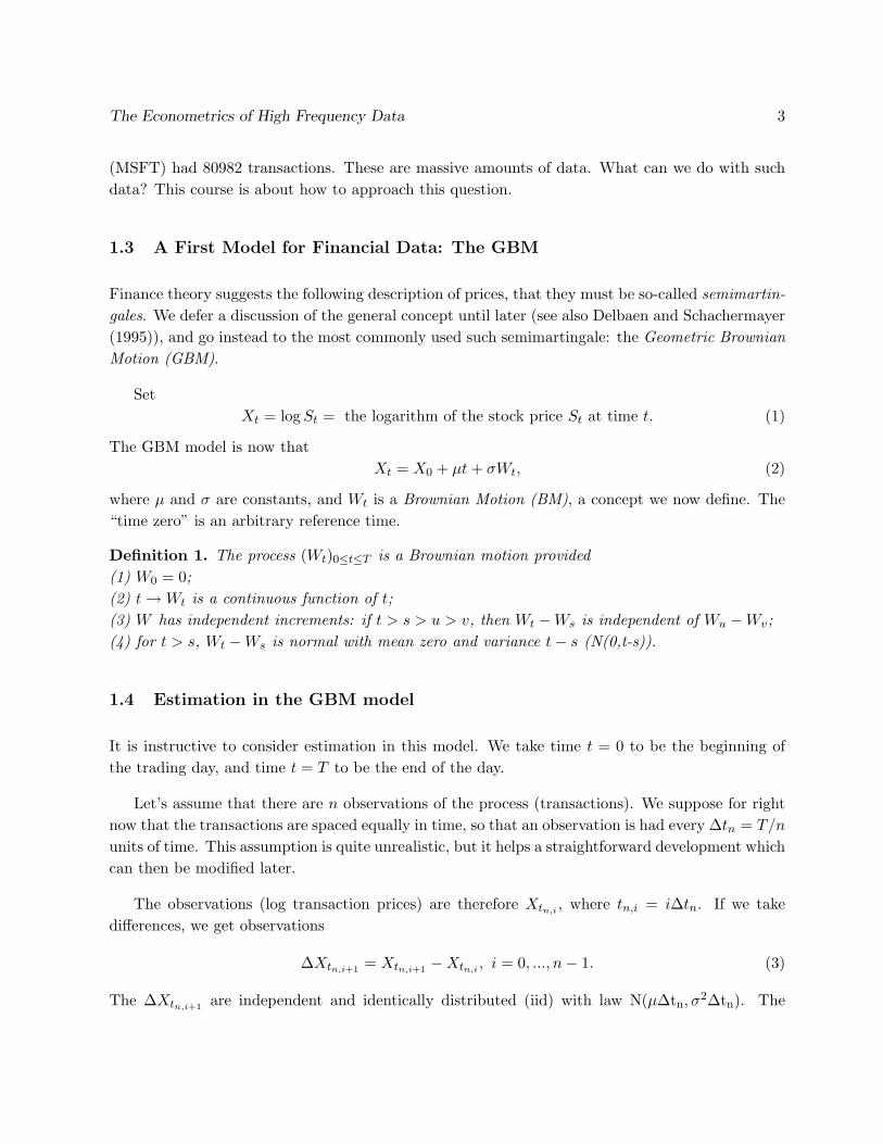
(MSFT) had 80982 transactions. These are massive amounts of data. What can we do with suchdata? This course is about how to approach this question.
1.3 A First Model for Financial Data: The GBM
Finance theory suggests the following description of prices, that they must be so-called semimartin-gales. We defer a discussion of the general concept until later (see also Delbaen and Schachermayer(1995)), and go instead to the most commonly used such semimartingale: the Geometric BrownianMotion (GBM).
SetXt = log St = the logarithm of the stock price St at time t. (1)
The GBM model is now thatXt = X0 + µt + σWt, (2)
where µ and σ are constants, and Wt is a Brownian Motion (BM), a concept we now define. The“time zero” is an arbitrary reference time.
Definition 1. The process (Wt)0≤t≤T is a Brownian motion provided(1) W0 = 0;(2) t → Wt is a continuous function of t;(3) W has independent increments: if t > s > u > v, then Wt −Ws is independent of Wu −Wv;(4) for t > s, Wt −Ws is normal with mean zero and variance t− s (N(0,t-s)).
1.4 Estimation in the GBM model
It is instructive to consider estimation in this model. We take time t = 0 to be the beginning ofthe trading day, and time t = T to be the end of the day.
Let’s assume that there are n observations of the process (transactions). We suppose for rightnow that the transactions are spaced equally in time, so that an observation is had every ∆tn = T/n
units of time. This assumption is quite unrealistic, but it helps a straightforward development whichcan then be modified later.
The observations (log transaction prices) are therefore Xtn,i , where tn,i = i∆tn. If we takedifferences, we get observations
∆Xtn,i+1 = Xtn,i+1 −Xtn,i , i = 0, ..., n− 1. (3)
The ∆Xtn,i+1 are independent and identically distributed (iid) with law N(µ∆tn, σ2∆tn). The
The Econometrics of High Frequency Data 4
natural estimators are:
µn =1
n∆tn
n−1∑i=0
∆Xtn,i+1 = (XT −X0)/T both MLE and UMVU; and
σ2n,MLE =
1n∆tn
n−1∑i=0
(∆Xtn,i+1 −∆Xtn)2 MLE; or (4)
σ2n,UMV U =
1(n− 1)∆tn
n−1∑i=0
(∆Xtn,i+1 −∆Xtn)2 UMVU.
Here, MLE is the maximum likelihood estimator, and UMVU is the uniformly minimum varianceunbiased estimator (see Lehmann (1983) or Rice (2006)). Also, ∆Xtn = 1
n
∑n−1i=0 ∆Xtn,i+1 = µn∆tn.
The estimators (4) clarify some basics. First of all, µ cannot be consistently estimated for fixedlength T of time interval. In fact, the µn does not depend on n, but only on T and the value ofthe process at the beginning and end of the time period. This is reassuring from a common senseperspective. If we could estimate µ for actual stock prices, we would be very rich!!! – Of course, ifT →∞, then µ can be estimated consistently.
It is perhaps more surprising that σ2 can be estimated consistently for fixed T , as n → ∞. Inother words, σ2
np→σ2 as n →∞. Set Un,i = ∆Xtn,i/(σ∆t
1/2n ). Then the Un,i are iid with distribution
N((µ/σ)∆t1/2n , 1). It follows from standard considerations for normal random variables that
n−1∑i=0
(Un,i − Un,·)2
is χ2 distributed with n− 1 degrees of freedom. Hence, for the UMVU estimator,
σ2n = σ2∆tn
1(n− 1)∆tn
n−1∑i=0
(Un,i − Un,·)2
= σ2 χ2n−1
n− 1.
It follows that
E(σ2n) = σ2 and Var(σ2
n) =σ4
n− 1, (5)
since Eχ2m = m and Var(χ2
m) = 2m. Hence σ2n is consistent for σ2: σ2
n → σ2 in probability asn →∞.
Similarly, since χ2n−1 is the sum of n− 1 iid χ2
1 random variables, by the central limit theoremwe have the following convergence in law:
χ2n−1 − Eχ2
n−1√Var(χ2
n−1)=
χ2n−1 − (n− 1)√
2(n− 1)L→ N(0, 1), (6)
The Econometrics of High Frequency Data 5
and so
n1/2(σ2n − σ2) ∼ (n− 1)1/2(σ2
n − σ2)
=√
2σ2 χ2n−1 − (n− 1)√
2(n− 1)L→ σ2N(0, 2) = N(0, 2σ4). (7)
This provides an asymptotic distribution which permits the setting of intervals. For example,σ2 = σ2
n ± 1.96×√
2σ2n would be an asymptotic 95 % confidence interval for σ2.
Since σ2n,MLE = n−1
n σ2n,UMV U , the same asymptotics apply to the MLE.
1.5 Behavior of Non-Centered Estimators
The above discussion of σ2n,UMV U and σ2
n,MLE is exactly the same as in the classical case of es-timating variance on the basis of iid observations. More unusually, for high frequency data, themean is often not removed in estimation. The reason is as follows. Set
σ2n,nocenter =
1n∆tn
n−1∑i=0
(∆Xtn,i+1)2. (8)
Now note that for the MLE version of σn,
σ2n,MLE =
1n∆tn
n−1∑i=0
(∆Xtn,i+1 −∆Xtn)2
=1
n∆tn
(n−1∑i=0
(∆Xtn,i+1)2 − n(∆Xtn)2
)= σ2
n,nocenter −∆tnµ2n
= σ2n,nocenter −
T
nµ2
n.
Since µ2n does not depend on n, it follows that
n1/2(σ2
n,MLE − σ2n,nocenter
) p→ 0.
Hence, σ2n,nocenter is consistent and has the same asymptotic distribution as σ2
n,UMV U and σ2n,MLE .
It can therefore also be used to estimate variance. This is quite common for high frequency data.
1.6 GBM and the Black-Scholes-Merton formula
The GBM model is closely tied in to other parts of finance. In particular, following the work ofBlack and Scholes (1973), Merton (1973), Harrison and Kreps (1979), and Harrison and Pliska
The Econometrics of High Frequency Data 6
(1981), precise option prices can be calculated in this model. See also Duffie (1996), Neftci (2000),Øksendal (2003), or Shreve (2004) for book sized introductions to the theory.
In the case of the call option, the price is as follows. A European call option on stock St withmaturity (expiration) time T and strike price K is the option to buy one unit of stock at price K
at time T . It is easy to see that the value of this option at time T is (ST −K)+, where x+ = x ifx ≥ 0, and x+ = 0 otherwise.
If we make the assumption that St is a GBM, which is to say that it follows (1)-(2), and alsothe assumption that the short term interest rate r is constant (in time), then the price at time t,0 ≤ t ≤ T of this option must be
price = C(St, σ2(T − t), r(T − t)), (9)
where
C(S, Ξ, R) = SΦ(d1)−K exp(−R)Φ(d2), where
d1,2 = (log(S/K) + R± Ξ/2) /√
Ξ and (10)
Φ(x) = P (N(0, 1) ≤ x) the standard normal cdf.
This is the Black-Scholes-Merton formula.
We shall see later on how high frequency estimates can be used in this formula. For the moment,note that the price only depends on quantities that are either observed (the interest rate r) or nearlyso (the volatility σ2). It does not depend on µ. Unfortunately, the assumption of constant r andσ2 is unrealistic, as we shall discuss in the following.
The GBM model is also heavily used in portfolio optimization
1.7 Our Problem to be Solved: Inadequacies in the GBM Model
We here give a laundry list of questions that arise and have to be dealt with.
1.7.1 The Volatility Depends on t
It is empirically the case that σ2 depends on t. We shall talk about the instantaneous volatility σ2t .
This concept will be defined carefully in Section 2.
1.7.2 The Volatility is Random; Leverage Effect
Returns are usually assumed to be non-normal. Such behavior can for the most part be modeledas σ2
t having random evolution. It is also usually assumed that σ2t can be correlated with the (log)
The Econometrics of High Frequency Data 7
stock price. This is often referred to as Leverage Effect. More about this in Section 2.
1.7.3 Jumps
The GBM model assumes that the log stock price Xt is continuous as a function of t. The evolutionof the stock price, however, is often thought to have a jump component. The treatment of jumpsis largely not covered in this article, though there is some discussion in Section 6.4.1, which alsogives some references. Note that jumps and random volatility are often confounded, since anymartingale can be embedded in a Brownian motion (Dambis (1965), Dubins and Schwartz (1965),see also Mykland (1995) for a review and further discussion).
1.7.4 Non-Normal Returns
Most non-normal behavior can be explained though random volatility and/or jumps. It would beunusual to need more extensive modeling.
1.7.5 Microstructure Noise
An important feature of actual transaction prices is the existence of microstructure noise. Transac-tion prices, as actually observed are typically best modeled on the form Yt = log St = the logarithmof the stock price St at time t, where for transaction at time ti,
Yti = Xti + noise, (11)
and Xt is a semimartingale. This is often called the hidden semimartingale model. This issue is animportant part of our narrative, and is further discussed in Section 5, see also Section 6.4.2.
1.7.6 Unequally Spaced Observations
In the above, we assumed that the transaction times ti are equally spaced. A quick glance at thedata snippet in Section 1.2 reveal that this is typically not the case. This leads to questions thatwill be addressed as we go along.
1.8 A Note on Probability Theory
We will extensively use probability theory in these notes. To avoid making a long introduction onstochastic processes, we will define concepts as we need them, but not always in the greatest depth.We will also omit other concepts and many basic proofs. As a compromise between the rigorous

The Econometrics of High Frequency Data 8
and the intuitive, we follow the following convention, that the notes will (except when the oppositeis clearly stated) use mathematical terms as they are defined in Jacod and Shiryaev (2003). Thus,in case of doubt, this work can be consulted.
Other recommended reference books on stochastic process theory are Karatzas and Shreve(1991), Øksendal (2003), Protter (2004), and Shreve (2004). For introduction to measure theoreticprobability, one can consult Billingsley (1995).
2 A More General Model: Time varying Drift and Volatility
2.1 Stochastic Integrals, Ito-Processes
We here make some basic definitions. We consider a process Xt, where the time variable t ∈ [0, T ].We mainly develop the univariate case here.
2.1.1 Information Sets, σ-fields, Filtrations
Information is usually described with so-called σ-fields. The setup is as follows. Our basic spaceis (Ω,F), where Ω is the set of all possible outcomes ω, and F is the collection of subsets A ⊆ Ωthat will eventually be decidable (it will be observed whether they occured or not). All randomvariables are thought to be a function of the basic outcome ω ∈ Ω.
We assume that F is a so-called σ-field. In general,
Definition 2. A collection A of subsets of Ω is a σ-field if
(i) ∅, Ω ∈ A;(ii) if A ∈ A, then Ac = Ω−A ∈ A; and(iii) if An, n = 1, 2, ... are all in A, then ∪∞n=1An ∈ A.
If one thinks of A as a collection of decidable sets, then the interpretation of this definition isas follows:
(i) ∅, Ω are decidable (∅ didn’t occur, Ω did);(ii) if A is decidable, so is the complement Ac (if A occurs, then Ac does not occur, and vice versa);(iii) if all the An are decidable, then so is the event ∪∞n=1An (the union occurs if and only if at leastone of the Ai occurs).
A random variable X is called A-measurable if the value of X can be decided on the basis of theinformation in A. Formally, the requirement is that for all x, the set X ≤ x = ω ∈ Ω : X(ω) ≤x be decidable (∈ A).

The Econometrics of High Frequency Data 9
The evolution of knowledge in our system is described by the filtration (or sequence of σ-fields)Ft, 0 ≤ t ≤ T . Here Ft is the knowledge available at time t. Since increasing time makes more setsdecidable, the family (Ft) is taken to satisfy that if s ≤ t, then Fs ⊆ Ft.
Most processes will be taken to be adapted to (Ft): (Xt) is adapted to (Ft) if for all t ∈ [0, T ],Xt is Ft-measurable. A vector process is adapted if each component is adapted.
We define the filtration (FXt ) generated by the process (Xt) as the smallest filtration to which
Xt is adapted. By this we mean that for any filtration F ′t to which (Xt) is adapted, FXt ⊆ F ′t for
all t. (Proving the existence of such a filtration is left as an exercise for the reader).
2.1.2 Wiener Processes
A Wiener process is Brownian motion relative to a filtration. Specifically,
Definition 3. The process (Wt)0≤t≤T is an (Ft)-Wiener process if it is adpted to (Ft) and(1) W0 = 0;(2) t → Wt is a continuous function of t;(3) W has independent increments relative to the filtration (Ft): if t > s, then Wt −Ws is inde-pendent of Fs;(4) for t > s, Wt −Ws is normal with mean zero and variance t− s (N(0,t-s)).
Note that a Brownian motion (Wt) is an (FWt )-Wiener process.
2.1.3 Predictable Processes
For defining stochastic integrals, we need the concept of predictable process. “Predictable” heremeans that one can forecast the value over infinitesimal time intervals. The most basic examplewould be a “simple process”. This is given by considering break points 0 = s0 ≤ s1 < t1 ≤ s2 <
t2 < ... ≤ sn < tn ≤ T , and random variables H(i), observable (measurable) with respect to Fsi .
Ht =
H(0) if t = 0H(i) if si < t ≤ ti
(12)
In this case, at any time t (the beginning time t = 0 is treated separately), the value of Ht is knownbefore time t.
Definition 4. More generally, a process Ht is predictable if it can be written as a limit of simplefunctions H
(n)t . This means that H
(n)t (ω) → Ht(ω) as n →∞, for all (t, ω) ∈ [0, T ]× Ω.
All adapted continuous processes are predictable. More generally, this is also true for adaptedprocesses that are left continuous (cag, for continue a gauche). (Proposition I.2.6 (p. 17) in Jacodand Shiryaev (2003)).
The Econometrics of High Frequency Data 10
2.1.4 Stochastic Integrals
We here consider the meaning of the expression∫ T
0HtdXt. (13)
The ingredients are the integrand Ht, which is assumed to be predictable, and the integrator Xt,which will generally be a semi-martingale (to be defined below in Section 2.3.5).
The expression (13) is defined for simple process integrands as∑i
H(i)(Xti −Xsi) (14)
For predictable integrands Ht that are bounded and limits of simple processes H(n)t , the integral
(13) is the limit in probability of∫ T0 H
(n)t dXt. This limit is well defined, i.e., independent of the
sequence H(n)t .
If Xt is a Wiener process, the integral can be defined for any predictable process Ht satisfying∫ T
0H2
t dt < ∞. (15)
It will always be the case that the integrator Xt is right continuous with left limits (cadlag, forcontinue a droite, limites a gauche).
The integral process ∫ t
0HsdXs =
∫ T
0HsIs ≤ tdXs (16)
can also be taken to be cadlag. If (Xt) is continuous, the integral is then automatically continuous.
2.1.5 Ito Processes
We now come to our main model, the Ito process. Xt is an Ito process relative to filtration (Ft)provided (Xt) is (Ft) adapted; and if there is an (Ft)-Wiener process (Wt), and (Ft)-adaptedprocesses (µt) and (σt), with ∫ T
0|µt|dt < ∞, and (17)∫ T
0σ2
t dt < ∞ (18)
so that
Xt = X0 +∫ t
0µsds +
∫ t
0σsdWs. (19)
The Econometrics of High Frequency Data 11
The process is often written on differential form:
dXt = µtdt + σtdWt. (20)
We note that the Ito process property is preserved under stochastic integration. If Ht is boundedand predictable, then ∫ t
0HsdXs =
∫ t
0Hsµsdt +
∫ t
0HsσsdWs. (21)
It is clear from this formula that predictable processes Ht can be used for integration w.r.t. Xt
provided ∫ T
0|Htµt|dt < ∞ and (22)∫ T
0(Htσt)2dt < ∞. (23)
2.2 Two Interpretations of the Stochastic Integral
One can use the stochastic integral in two different ways: as model, or as a description of tradingprofit and loss (P/L).
2.2.1 Stochastic Integral as Trading Profit and Loss
Suppose that Xt is the value of a security. Let Ht be the number of this stock that is held at timet. In the case of a simple process (12), this means that we hold H(i) units of X from time si totime ti. The trading P/L is then given by the stochastic integral (14). In this description, it isquite clear that H(i) must be known at time si, otherwise we would base the portfolio on futureinformation. More generally, for predictable Ht, we similarly avoid using future information.
2.2.2 Stochastic Integral as Model
This is a different genesis of the stochastic integral model. One simply uses (19) as a model, inthe hope that this is a sufficiently general framework to capture most relevant processes. Theadvantage of using predictable integrands come from the simplicity of connecting the model withtrading gains.
For simple µt and σ2t , the integral∑
i
µ(i)(ti − si) +∑
i
σ(i)(Wti −Wsi) (24)

The Econometrics of High Frequency Data 12
is simply a sum of contitionally normal random variables, with mean µ(i)(ti − si) and variance(σ(i))2(ti − si). The sum need not be normal, since µ and σ2 can be random.
It is worth noting that in this model,∫ T0 µtdt is the sum of instantaneous means (drift), and∫ T
0 σ2t dt is the sum of intstantaneous variances. In fact, in the model (19), one can show the
following: Let Var(·|Ft) be the conditional variance given the information at time t. If Xt is an Itoprocess, and if 0 = tn,0 < tn,i < ... < tn,n = T , then
∑i
Var(Xtn,i+1 −Xtn,i |Ftn,i)p→∫ T
0σ2
t dt (25)
whenmax
i|tn,i+1 − tn,i| → 0. (26)
If the µt and σ2t processes are nonrandom, then Xt is a Gaussian process, and XT is normal
with mean X0 +∫ T0 µtdt and variance
∫ T0 σ2
t dt.
2.2.3 The Heston model
A popular model for volatility is due to Heston (1993). In this model, the process Xt is given by
dXt = µdt + σtdWt
dσ2t = κ(α− σ2
t )dt + γσtdZt , with (27)
Zt = ρWt + (1− ρ2)1/2Bt (28)
where (Wt) and (Bt) are two independent Wiener processes, κ > 0, and |ρ| ≤ 1.
2.3 Semimartingales
2.3.1 Conditional Expectations
Denote by E(·|Ft) the conditional expectation given the information available at time t. Formally,this concept is defined as follows:
Theorem 1. Let A be a σ-field, and let X be a random variable so that E|X| < ∞. There is aA-measurable random variable Z so that for all A ∈ A,
EZIA = EXIA, (29)
where IA is the indicator function of A. Z is unique “almost surely”, which is that if Z1 and Z2
satisfy the two criteria above, then P (Z1 = Z2) = 1.
The Econometrics of High Frequency Data 13
We thus defineE(X|A) = Z (30)
where Z is given in the theorem. The conditional expectation is well defined “almost surely”.
For further details and proof of theorem, see Section 34 (p. 445-455) of Billingsley (1995).
This way of defining conditional expectation is a little counterintuitive if unfamiliar. In partic-ular, the conditional expectation is a random variable. The heuristic is as follows. Suppose thatY is a random variable, and that A carries the information in Y . Introductory textbooks oftenintroduce conditional expectation as a non-random quantity E(X|Y = y). To make the connection,set
f(y) = E(X|Y = y). (31)
The conditional expectation we have just defined then satisfies
E(X|A) = f(Y ). (32)
2.3.2 Properties of Conditional Expectations
• Linearity: for constant c1, c2:
E(c1X1 + c2X2 | A) = c1E(X1 | A) + c2E(X2 | A)
• Conditional constants: if Z is A-measurable, then
E(ZX|A) = ZE(X|A)
• Law of iterated expectations (iterated conditioning, tower property): if A′ ⊆ A, then
E[E(X|A)|A′] = E(X|A′)
• Independence: if X is independent of A:
E(X|A) = E(X)
• Jensen’s inequality: if g : x → g(x) is convex:
E(g(X)|A) ≥ g(E(X|A))
Note: g is convex if g(ax + (1− a)y) ≤ ag(x) + (1− a)g(y) for 0 ≤ a ≤ 1. For example: g(x) = ex,
g(x) = (x−K)+. Or g′′ exists and is continuous, and g′′(x) ≥ 0.

The Econometrics of High Frequency Data 14
2.3.3 Martingales
An (Ft) adapted process Mt is called a martingale if E|Mt| < ∞, and if, for all s < t,
E(Mt|Fs) = Ms. (33)
This is a central concept in our narrative. A martingale is also known as a fair game, for thefollowing reason. In a gambling situation, if Ms is the amount of money the gambler has at times, then the gambler’s expected wealth at time t > s is also Ms. (The concept of martingale appliesequally to discrete and continuous time axis).
Example 1. A Wiener process is a martingale. To wit, for t > s, since Wt−Ws is N(0,t-s) givenFs, we get that
E(Wt|Fs) = E(Wt −Ws|Fs) + Ws
= E(Wt −Ws) + Ws by independence
= Ws. (34)
A useful fact about martingales is the representation by final value: Mt is a martingale for0 ≤ t ≤ T if and only if one can write
Mt = E(X|Ft) for all t ∈ [0, T ] (35)
(only if by definition (X = MT ), if by Tower property). Note that for T = ∞ (which we do notconsider here), this property may not hold. (For a full discussion, see Chapter 1.3.B (p. 17-19) ofKaratzas and Shreve (1991)).
Example 2. If Ht is a bounded predictable process, and for any martingale Xt,
Mt =∫ t
0HsdXs (36)
is a martingale. To see this, consider first a simple process (12), for which Ht = H(i) whensi < t ≤ ti. For given t, if si > t, by the properties of conditional expectations,
E(H(i)(Xti −Xsi)|Ft
)= E
(E(H(i)(Xti −Xsi)|Fsi)|Ft
)= E
(H(i)E(Xti −Xsi |Fsi)|Ft
)= 0, (37)
and similarly, if ti ≤ t ≤ si, then
E(H(i)(Xti −Xsi)|Ft
)= H(i)(Xt −Xsi) (38)
The Econometrics of High Frequency Data 15
so that
E(MT |Ft) = E
(∑i
H(i)(Xti −Xsi)|Ft
)=∑
i:ti<t
H(i)(Xti −Xsi) + Iti ≤ t ≤ siH(i)(Xt −Xsi)
= Mt. (39)
The result follows for general bounded predicable integrands by taking limits and using uniformintegrability. (For definition and results on uniform integrability, see Billingsley (1995).)
Thus, any bounded trading strategy in a martingale results in another martingale.
2.3.4 Stopping Times and Local Martingales
The concept of local martingale is perhaps best understood by considering the following integralwith respect to a Wiener process (see also Duffie (1996)):
Xt =∫ t
0
1√T − s
dWs (40)
Note that for 0 ≤ t < T , Xt is a zero mean Gaussian process with independent increments. Weshall show below (in Section 2.4.3) that the integral has variance
Var(Xt) =∫ t
0
1T − s
ds
=∫ T
T−t
1u
du
= logT
T − t. (41)
Since the spread of Xt goes to infinity as we approach T , Xt is not defined at T . However, one canstop the process at a convenient time, as follows: Set, for A > 0,
τ = inft ≥ 0 : Xt = A. (42)
One can show that P (τ < T ) = 1. Define the modified integral by
Yt =∫ t
0
1√T − s
Is ≤ τdWs
= Xτ∧t, (43)
wheres ∧ t = min(s, t). (44)

The Econometrics of High Frequency Data 16
The process (43) has the following trading interpretation. Suppose that Wt is the value of asecurity at time t (the value can be negative, but that is possible for many securities, such asfutures contracts). We also take the short term interest rate to be zero. The process Xt comesabout as the value of a portfolio which holds 1/
√T − t units of this security at time t. The process
Yt is obtained by holding this portfolio until such time that Xt = A, and then liquidating theportfolio.
In other words, we have displayed a trading strategy which starts with wealth Y0 = 0 at timet = 0, and end with wealth YT = A > 0 at time t = T . In trading terms, this is an arbitrage. Inmathematical terms, this is a stochastic integral w.r.t. a martingale which is no longer a martingale.
We note that from (41), the condition (15) for the existence of the integral is satisfied.
For trading, the lesson we can learn from this is that some condition has to be imposed to makesure that a trading strategy in a martingale cannot result in arbitrage profit. The most popularapproach to this is to require that the traders wealth at any time cannot go below some fixedamount −K. This is the so-called credit constraint. (So strategies are required to satisfy that theintegral never goes below −K). This does not quite guarantee that the integral w.r.t. a martingaleis a martingale, but it does prevent arbitrage profit. The technical result is that the integral is asuper-martingale (see the next section).
For the purpose of characterizing the stochastic integral, we need the concept of a local martin-gale. For this, we first need to define:
Definition 5. A stopping time is a random variable τ satisfying τ ≤ t ∈ Ft, for all t.
The requirement in this definition is that we must be able to know at time t wether τ occurredor not. The time (42) given above is a stopping time. On the other hand, the variable τ =inft : Wt = max0≤s≤T Ws is not a stopping time. Otherwise, we would have a nice investmentstrategy.
Definition 6. A process Mt is a local martingale for 0 ≤ t ≤ T provided there is a sequence ofstopping times τn so that(i) Mτn∧t is a martingale for each n
(ii) P (τn = T ) → 1 as n →∞.
The basic result for stochastic integrals is now that the integral with respect to a local martingaleis a local martingale, cf. result I.4.34(b) (p. 47) in Jacod and Shiryaev (2003).
2.3.5 Semimartingales
Xt is a semimaringtale if it can be written
Xt = X0 + Mt + At, 0 ≤ t ≤ T, (45)

The Econometrics of High Frequency Data 17
where X0 is F0-measurable, Mt is a local martingale, and At is a process of finite variation, i.e.,
sup∑
i
|Xti+1 −Xti | < ∞, (46)
where the supremum is over all grids 0 = t0 < t1 < ... < tn = T , and all n.
In particular, an Ito process is a semimartingale, with
Mt =∫ t
0σtdWt and
At =∫ t
0µtdt. (47)
A supermartingale is semimartingale for which At is nonincreasing. A submartingale is a semi-martingale for which At is nondecreasing.
2.4 Quadratic Variation of a Semimartingale
2.4.1 Definitions
We start with some notation. A grid of observation times is given by
G = t0, t1, ..., tn, (48)
where we suppose that0 = t0 < t1 < ... < tn = T. (49)
Set∆(G) = max
1≤i≤n(ti − ti−1). (50)
For any process X, we define its quadratic variation relative to grid G by
[X, X]Gt =∑
ti+1≤t
(Xti+1 −Xti)2. (51)
One can more generally define the quadratic covariation
[X, Y ]Gt =∑
ti+1≤t
(Xti+1 −Xti)(Yti+1 − Yti). (52)
An important theorem of stochastic calculus now says that
Theorem 2. For any semimartingale, there is a process [X, Y ]t so that
[X, Y ]Gtp→[X, Y ]t for all t ∈ [0, T ], as ∆(G) → 0. (53)
The limit is independent of the sequence of grids G.
The Econometrics of High Frequency Data 18
The result follows from Theorem I.4.47 (p. 52) in Jacod and Shiryaev (2003). In fact, theti can even be stopping times. (In our further development, the ti will typically be irregular butnonrandom).
For an Ito process,
[X, X]t =∫ t
0σ2
sds. (54)
(Cf Thm I.4.52 (p. 55) and I.4.40(d) (p. 48) of Jacod and Shiryaev (2003)).
The process [X, X]t is usually referred to as the quadratic variation of the semimartingale (Xt).This is an important concept, as seen in Section 2.2.2. The theorem asserts that this quantity canbe estimated consistently from data.
2.4.2 Properties
Important properties are as follows:
(1) Bilinearity: [X, Y ]t is linear in each of X and Y .
(2) If (Wt) and (Bt) are two independent Wiener processes, then
[W,B]t = 0. (55)
Example 3. For the Heston model in Section 2.2.3, one gets from first principles that
[W,Z]t = ρ[W,W ]t + (1− ρ2)1/2[W,B]t= ρt, (56)
since [W,W ]t = t and [W,B]t = 0.
(3) For stochastic integrals over Ito processes Xt and Yt,
Ut =∫ t
0HsdXs and Vt =
∫ t
0KsdYs, (57)
then
[U, V ]t =∫ t
0HsKsd[X, Y ]s. (58)
This is often written on “differential form” as
d[U, V ]t = HtKtd[X, Y ]t. (59)
by invoking the same results that led to (54).
(4) For any Ito process X, [X, t] = 0.

The Econometrics of High Frequency Data 19
Example 4. (Leverage Effect in the Heston model).
d[X, σ2] = γσ2t d[W,Z]t
= γσ2ρdt. (60)
(5) Invariance under discounting by the short term interest rate. Discounting is important infinance theory. The typical discount rate is the risk free short term interest rate rt. Recall thatSt = expXt. The discounted stock price is then given by
S∗t = exp−∫ t
0rsdsSt. (61)
The corresponding process on the log scale is X∗t = Xt−
∫ t0 rsds, so that if Xt is given by (20), then
dX∗t = (µt − rt)dt + σtdWt. (62)
The quadratic variation of X∗t is therefore the same as for Xt.
It should be emphasized that while this result remains true for certain other types of discounting(such as those incorporating cost-of-carry), it is not true for many other relevant types of discount-ing. For example, if one discounts by the zero coupon bond Λt maturing at time T , the discountedlog price becomes X∗
t = Xt − log Λt. Since the zero coupon bond will itself have volatility, we get
[X∗, X∗]t = [X, X]t + [log Λ, log Λ]t − 2[X, log Λ]t. (63)
2.4.3 Variance and Quadratic Variation
Quadratic variation has a representation in terms of variance. The main result concerns martingales.For E(X2) < ∞, define the conditional variance by
Var(X|A) = E((X− E(X|A))2|A) = E(X2|A)− E(X|A)2. (64)
and similarly Cov(X,Y|A) = E((X− E(X|A))(Y − E(Y|A)|A).
Theorem 3. Let Mt be a martingale, and assume that E[M,M ]T < ∞. Then, for all s < t,
Var(Mt|Fs) = E((Mt −Ms)2|Fs) = E([M,M]t − [M,M]s|Fs). (65)
A quick argument for this is as follows. Let G = t0, t1, ..., tn, and suppose for simplicity thats, t ∈ G. Then, for s ≤ ti < tj ,
E((Mti+1 −Mti)(Mtj+1 −Mtj )|Ftj ) = (Mti+1 −Mti)E((Mtj+1 −Mtj )|Ftj )
= 0, (66)
The Econometrics of High Frequency Data 20
so that by the Tower rule (since Fs ⊆ Ftj )
Cov(Mti+1 −Mti ,Mtj+1 −Mtj |Fs) = E((Mti+1 −Mti)(Mtj+1 −Mtj)|Fs) = 0. (67)
If follows that
Var(Mt −Ms|Fs) =∑
s≤ti<t
Var(Mti+1 −Mti |Fs)
=∑
s≤ti<t
E((Mti+1 −Mti)2|Fs)
= E(∑
s≤ti<t
(Mti+1 −Mti)2|Fs)
= E([M,M ]Gt − [M,M ]Gs |Fs). (68)
The result as ∆(G) → 0 then follows by uniform integrability (Theorem 25.12 (p. 338) in Billingsley(1995)).
On the basis of this, one can now show for an Ito process that
limh↓0
1h
Cov(Xt+h −Xt,Yt+h −Yt|Ft) =ddt
[X,Y]t. (69)
A similar result holds in the integrated sense, cf. formula (25). The reason this works is that thedt terms are of smaller order than the martingale terms.
Sometimes instantaneous correlation is important. We define
cor(X,Y)t = limh↓0
cor(Xt+h −Xt,Yt+h −Yt|Ft), (70)
and note thatcor(X,Y)t =
d[X,Y]t/dt√(d[X,X]t/dt)(d[Y,Y]t/dt)
. (71)
We emphasize that these results only hold for Ito processes. For general semimartingales, one needsto involve the concept of predictable quadratic variation, cf. Section 2.4.5.
To see the importance of the instantaneous correlation, note that in the Heston model,
cor(X, σ2)t = ρ. (72)
In general, if dXt = σtdWt +dt-term, and dYt = γtdBt +dt-term, where Wt and Bt are two Wienerprocesses, then
cor(X,Y)t = sgn(σtγt)cor(W,B)t. (73)
The Econometrics of High Frequency Data 21
2.4.4 Levy’s Theorem
A important result is now the following:
Theorem 4. Suppose that Mt is a continuous (Ft)-local martingale, M0 = 0, so that [M,M ]t = t.Then Mt is an (Ft)-Wiener process.
(Cf. Thm II.4.4 (p. 102) in Jacod and Shiryaev (2003)). More generally, from properties ofnormal random variables, the same result follows in the vector case: If Mt = (M (1)
t , ...,M(p)t ) is
a continuous (Ft)-martingale, M0 = 0, so that [M (i),M (j)]t = δijt, then Mt is a vector Wienerprocess. (δij is the Kronecker delta: δij = 1 for i = j, and = 0 otherwise.)
2.4.5 Predictable Quadratic Variation
One can often see the symbol 〈X, Y 〉t.This can be called the predictable quadratic vartiation. Underregularity conditions, it is defined as the limit of
∑ti≤t Cov(Xti+1−Xti ,Yti+1−Yti |Fti) as ∆(G) → 0.
For Ito processes, 〈X, Y 〉t = [X, Y ]t. For general semimartingales this equality does not hold.Also, except for Ito processes, 〈X, Y 〉t cannot generally be estimated consistently from data withoutfurther assumptions.
The symbol 〈X, Y 〉t is commonly used in the literature (including in our papers).
2.5 Ito’s Formula for Ito processes
2.5.1 Main Theorem
Theorem 5. Suppose that f is a twice continuously differentiable function, and that Xt is an Itoprocess. Then
df(Xt) = f ′(Xt)dXt +12f ′′(Xt)d[X, X]t. (74)
Similarly, in the multivariate case, for Xt = (X(1)t , ..., X
(p)t ),
df(Xt) =p∑
i=1
∂f
∂x(i)(Xt)dX
(i)t +
12
p∑i,j=1
∂2f
∂x(i)∂x(j)(Xt)d[X(i), X(j)]t. (75)
(Reference: Theorem I.4.57 in Jacod and Shiryaev (2003).)
We emphasize that (74) is the same as saying that
f(Xt) = f(X0) +∫ t
0f ′(Xs)dXs +
12
∫ t
0f ′′(Xs)d[X, X]s. (76)
The Econometrics of High Frequency Data 22
If we write out dXt = µtdt + σtdWt and d[X, X]t = σ2t dt, then equation (74) becomes
df(Xt) = f ′(Xt)(µtdt + σtdWt) +12f ′′(Xt)σ2
t dt
= (f ′(Xt)µt +12f ′′(Xt)σ2
t )dt + f ′(Xt)σtdWt. (77)
We note, in particular, that if Xt is an Ito process, then so is f(Xt).
2.5.2 Example of Ito’s Formula: Stochastic Equation for a Stock Price
We have so far discussed the model for a stock on the log scale, as dXt = µtdt + σtdWt. The priceis given as St = exp(Xt). Using Ito’s formula, with f(x) = exp(x), we get
dSt = St(µt +12σ2
t )dt + StσtdWt. (78)
2.5.3 Example of Ito’s Formula: Genesis of the Leverage Effect
We here see a case where quadratic covariation between a process and it’s volatility can arise frombasic economic principles. The following is the origin of the use of the word “leverage effect”to describe such covariation. We emphasize that this kind of covaration can arise from manyconsideration, and will later use the term leverage effect to describe the phenomenon broadly.
Suppose that the log value of a firm is Zt, given as a GBM,
dZt = νdt + γdWt. (79)
For simplicity, suppose that the interest rate is zero, and that the firm has borrowed C dollars (oreuros, yuan, ...). If there are M shares in the company, the value of one share is therefore
St = (exp(Zt)− C)/M. (80)
On the log scale, therefore, by Ito’s Formula,
dXt = d log(St)
=1St
dSt −12
1S2
t
d[S, S]t
=M
exp(Zt)− CdSt −
12
(M
exp(Zt)− C
)2
d[S, S]t
Since, in the same way as for (78)
dSt =1M
d exp(Zt)
=1M
exp(Zt)[(ν +12γ2)dt + γdWt]. (81)

The Econometrics of High Frequency Data 23
Hence, if we set
Ut =exp(Zt)
exp(Zt)− C, (82)
dXt = Ut[(ν +12γ2)dt + γdWt]−
12U2
t γdt
= (νUt +12γ2(Ut − U2
t ))dt + UtγdWt. (83)
In other words,dXt = µtdt + σ2
t dWt (84)
where
µt = νUt +12γ2(Ut − U2
t ) and
σt = Utγ. (85)
In this case, the log stock price and the volatility are, indeed, correlated. When the stock price goesdown, the volatility goes up (and the volatility will go to infinity if the value of the firm approachesthe borrowed amount C, since in this case Ut → ∞. In terms of quadratic variation, the leverageeffect is given as
d[X, σ2]t = Utγ3d[W,U2]t
= 2U2t γ3d[W,U ]t since dU2
t = 2UtdUt + d[U,U ]t= −2U4
t γ4C exp(−Zt)dt (86)
The last transition follows since, by taking f(x) = (1− C exp(−x))−1
dUt = df(Zt)
= f ′(Zt)dZt + dt-terms (87)
so that
d[W,U ]t = f ′(Zt)d[W,Z]t= f ′(Zt)γdt
= −U2t C exp(−Zt)γdt, (88)
since f ′(x) = −f(x)2C exp(−x).
A perhaps more intuitive result is obtained from (73), by observing that sgn(d[X, σ2]t/dt) = −1:on the correlation scale, the leverage effect is
cor(X, σ2)t = −1. (89)
The Econometrics of High Frequency Data 24
2.6 Nonparametric Hedging of Options
Suppose we can set the following prediction intervals at time t = 0:
R+ ≥∫ T
0rudu ≥ R− and Ξ+ ≥
∫ T
0σ2
udu ≥ Ξ− (90)
Is there any sense that we can hedge an option based on this interval?
We shall see that for a European call there is a strategy, beginning with wealth C(S0,Ξ+, R+),which will be solvent for the option payoff so long as the intervals in (90) are realized.
First note that by direct differentiation in (10), one obtains the two [sic] Black-Scholes-Mertondifferential equations
12CSSS2 = CΞ and − CR = C − CSS (91)
(recall that C(S, Ξ, R) = SΦ(d1)−K exp(−R)Φ(d2) and d1,2 = (log(S/K) + R± Ξ/2) /√
Ξ).
In analogy with Section 1.6, consider the instrument with price at time t:
Vt = C(St,Ξt, Rt, ), (92)
where
Rt = R+ −∫ t
0rudu and Ξt = Ξ+ −
∫ t
0σ2
udu (93)
We shall see that the instrument Vt can be self financed by holding, at each time t,
CS(St,Ξt, Rt) units of stock, in other words StCS(St,Ξt, Rt) $ of stock, and
Vt − StCS(St,Ξt, Rt) = −CR(St,Ξt, Rt) $ in bonds . (94)
where the equality follows from the first equation in (91). Note first that, from Ito’s formula,
dVt = dC(St,Ξt, Rt)
= CSdSt + CRdRt + CΞdΞt +12CSSd[S, S]t
= CSdSt − CRrtdt− CΞσ2t dt +
12CSSS2
t σ2t dt
= CSdSt − CRrtdt (95)
because of the second equation in (91).
From equation (95), we see that holding CS units of stock, and −CR $ of bonds at all times t
does indeed produce a P/L Vt − V0, so that starting with V0 $ yields Vt $ at time t.
From the second equation in (94), we also see that Vt $ is exactly the amount needed to maintainthese positions in stock and bond. Thus, Vt has a self financing strategy.
The Econometrics of High Frequency Data 25
Estimated volatility can come into this problem in two ways:
(1) In real time, to set the hedging coefficients: under discrete observation, use
Ξt = Ξ+ − estimate of integrated volatility from 0 to t. (96)
(2) As an element of a forecasting procedure, to set intervals of the form (90).
For further literature on this approach, consult Mykland (2000, 2003a,b, 2005, 2009). The latterpaper discusses, among other things, the use of this method for setting reserve requirements basedon an exit strategy in the event of model failure.
For other ways of using realized volatility and similar estimators in options trading, we refer toZhang (2001), Hayashi and Mykland (2005), and Mykland and Zhang (2008).
3 Behavior of Estimators: Variance
3.1 The Emblematic Problem: Estimation of Volatility
In this section, we develop the tools to show convergence in high frequency data. As examplethroughout, we consider the problem of estimation of volatility. (In the absence of microstructure.)This classical problem is that of estimating
∫ t0 σ2
sds. The standard estimator, Realized Volatility(RV), is simply [X, X]Gt . The estimator is consistent as ∆(G) → 0, from the very definition ofquadratic variation.
This raises the question of what other properties one can associate with this estimator. Forexample, does the asymptotic normality continue to hold. This is a rather complex matter, as weshall see.
There is also the question of what to do in the presence microstructure, to which we return inSection 5.
3.2 A Local Martingale Assumption
For now consider the case where
Xt = X0 +∫ t
0σsdWs, (97)
i.e., Xt is a local martingale. We shall see in Section 4.4.5 that drift terms can easily be incorporatedinto the analysis.
We shall also, for now, assume that σt is bounded, i.e., there is a nonrandom σ+ so that
σ2t ≤ σ2
+ for all t. (98)

The Econometrics of High Frequency Data 26
This makes Xt a martingale. We shall see in Section 4.5 how to remove this assumption.
3.3 The Error Process
On a grid G = t0, t1, ..., tn, we get from Ito’s formula that
(Xti+1 −Xti)2 = 2
∫ ti+1
ti
(Xs −Xti)dXs +∫ ti+1
ti
σ2sds. (99)
If we sett∗ = maxti ∈ G : ti ≤ t, (100)
the same equation will hold with (t∗, t) replacing (ti, ti+1). Hence
Mt =∑
ti+1≤t
(Xti+1 −Xti)2 + (Xt −Xt∗)
2 −∫ t
0σ2
sds (101)
is a local martingale on the form
Mt = 2∑
ti+1≤t
∫ ti+1
ti
(Xs −Xti)dXs + 2∫ t
t∗
(Xs −Xt∗)dXs. (102)
We shall study the behavior of martingales such as Mt.
Of course, we only observe [X, X]Gt =∑
ti+1≤t(Xti+1 − Xti)2, but we shall see next that the
same results apply to this quantity. ((Xt −Xt∗)2 is negligible.)
3.4 Stochastic Order Symbols
We also make use of the following notation:
Definition 7. (stochastic order symbols) Let Zn be a sequence of random variables. We say thatZn = op(1) if Zn → 0 in probability, and that Zn = op(un) if Zn/un = op(1). Similarly, we saythat Zn = Op(1) if for all ε > 0, there is an M so that supn P (|Zn| > M) ≤ ε. This is the same assaying that for every subsequence nk, there is a further subsequence nkl
so that Znklconverges in
law. (see Theorem 29.3 (p. 380) in Billingsley (1995)). Finally, Zn = Op(un) if Zn/un = Op(1).
For further discusion of this notation, see the Appendix A in Pollard (1984). (This book is outof print, but can at the time of writing be downloaded from http://www.stat.yale.edu/ pollard/).
The Econometrics of High Frequency Data 27
To see an illustration of the usage: under (98), we have that
E(Xt −Xt∗)2 = E([X, X]t − [X, X]t∗)
= E
∫ t
t∗
σ2sds
≤ E(t− t∗)σ2+
≤ E∆(G)σ2+ (103)
so that (Xt −Xt∗)2 = Op(∆(G)).
3.5 Quadratic Variation of the Error Process: Approximation by Quarticity
3.5.1 An Important Result
To find the variance of our estimate, we start by computing the quadratic variation
[M,M ]Gt = 4∑
ti+1≤t
∫ ti+1
ti
(Xs −Xti)2d[X, X]s + 4
∫ t
t∗
(Xs −Xt∗)2d[X, X]s. (104)
A nice result, originally due to Barndorff-Nielsen and Shephard (2002), concerns the estimationof this variation. Define the quarticity by
[X, X, X, X]Gt =∑
ti+1≤t
(Xti+1 −Xti)4 + (Xt −Xt∗)
4 (105)
Use Ito’s formula to see that (where Mt is the error process from Section 3.3)
d(Xt −Xti)4 = 4(Xt −Xti)
3dXt + 6(Xt −Xti)2d[X, X]t
= 4(Xt −Xti)3dXt +
64d[M,M ]t, (106)
since d[M,M ]t = 4(Xt −Xti)2d[X, X]t. It follows that if we set
M(2)t =
∑ti+1≤t
∫ ti+1
ti
(Xs −Xti)3dXs +
∫ t
t∗
(Xs −Xt∗)3dXs (107)
we obtain[X, X, X, X]Gt =
32[M,M ]t + 4M
(2)t . (108)
It turns out that the M(2)t term is of order op(n−1), so that (2/3)n[X, X, X, X]Gt is a consistent
estimate of the quadratic variation (104):
The Econometrics of High Frequency Data 28
Proposition 1. Assume (98). Also suppose that, as n → 0, ∆(G) = op(1), and
n−1∑i=0
(ti+1 − ti)3 = Op(n−2). (109)
Thensup
0≤t≤T| [M,M ]t −
23[X, X, X, X]Gt | = op(n−1) as n →∞. (110)
3.5.2 The Conditions on the Times – Why They are Reasonable
Example 5. We first provide a simple example to emphasize that Proposition 1 does the rightthing. Assume for simplicity that the observation times are equidistant: ti = tn,i = iT/n, and thatthe volatility is constant: σt ≡ σ. It is then easy to see that the conditions, including (109), aresatisfied. On the other hand, [X, X, X, X]Gt has the distribution of (T/n)2σ4
∑ni=1 U4
i , where theUi are iid standard normal. Hence, n2
3 [X, X, X,X]Gtp→2
3T 2σ4E(N(0, 1)4) = 2T 2σ4. It then followsfrom Proposition 1 that n[M,M ]Gt
p→2T 2σ4.
Example 6. To see more generally why (109) is a natural condition, consider a couple of casesfor the spacings.(i) The spacings are sufficiently regular to satisfy
∆(G) = maxi
(ti+1 − ti) = Op(n−1). (111)
Thenn∑
i=0
(ti+1 − ti)3 ≤n∑
i=0
(ti+1 − ti)(
maxi
(ti+1 − ti))2
= T ×Op(n−2) (112)
(ii) On the other hand, suppose that the sampling times follow a Poisson process with parameter λ.If one conditions on the number of sampling points n, these points behave like the order statistics ofn uniformly distributed random variables (see, for example, Chapter 2.3 in Ross (1996)). In otherwords, ti = TU(i) (for 0 < i < n), where U(i) is the i’th order statistic of U1, ..., Un, which are iidU[0,1]. Hence the expression in (109) becomes (taking U(0) = 0 and U(n) = 1)
n−1∑i=0
(ti+1 − ti)3 = T 3n∑
i=1
(U(i) − U(i−1))3
= T 3nEU3(1)(1 + op(1)) (113)
by the law of large numbers, since the spacings have identical distribution [verify this]. SinceEU3
(1) = O(n−3), (109) follows.

The Econometrics of High Frequency Data 29
3.6 Moment Inequalities, and Proof of Proposition 1
3.6.1 Lp Norms, Moment Inequalities, and the Burkholder-Davis-Gundy Inequality
For 1 ≤ p < ∞, define the Lp-norm:
||X||p = (E|X|p)1p , (114)
The Minkowski and Holder inequalities say that
||X + Y ||p ≤ ||X||p + ||Y ||p
||XY ||1 ≤ ||X||p||Y ||q for1p
+1q
= 1. (115)
Example 7. A special case of the Holder inequalitiy is ||X||1 ≤ ||X||p (take Y = 1). In particular,under (109), for for 1 ≤ v ≤ 3:(
1n
n∑i=0
(ti+1 − ti)v
) 1v
≤
(1n
n∑i=0
(ti+1 − ti)3) 1
3
=(
1n×Op(n−2)
) 13
=(Op(n−3)
) 13 = Op(n−1), (116)
so thatn∑
i=0
(ti+1 − ti)v = Op(n1−v). (117)
To show Proposition 1, we need the Burkholder-Davis-Gundy inequality (see Section 3 of Ch.VII of Dellacherie and Meyer (1982), or p. 193 and 222 in Protter (2004)), as follows. For 1 ≤ p <
∞, there are universal constants cp and Cp so that for all continuous martingales Nt,
cp||[N,N ]T ||1/2p/2 ≤ || sup
0≤t≤T|Nt| ||p ≤ Cp||[N,N ]T ||1/2
p/2. (118)
Note, in particular, that for 1 < p < ∞,
C2p = qp
(p(p− 1)
2
)(119)
where q is given by p−1 + q−1 = 1.
3.6.2 Proof of Proposition 1
From Ito’s Formula:
[M (2),M (2)]t =∑
ti+1≤t
∫ ti+1
ti
(Xs −Xti)6d[X, X]s +
∫ t
t∗
(Xs −Xt∗)6d[X, X]s
=128
[X; 8]Gt + martingale term (120)
The Econometrics of High Frequency Data 30
where [X; 8]Gt =∑
ti+1≤t(Xti+1 −Xti)8 + 1
28(Xt −Xt∗)8 is the ochticity.
Note that for stopping time τ ≤ T , [X; 8]Gτ =∑
i(Xti+1∧τ −Xti∧τ )8. Hence, by the Burkholder-Davis-Gundy inequality (with p = 8)
E[M (2),M (2)]τ =128
E[X; 8]Gτ
≤ 128
C88E∑
i
([X, X]ti+1∧τ − [X, X]ti∧τ )4
≤ 128
C88σ8
+E∑
i
(ti+1 ∧ τ − ti ∧ τ)4. (121)
Let ε > 0, and setτn = inf t ∈ [0, T ] : n−2
∑i
(ti+1 ∧ t− ti ∧ t)4 > ε .
ThenE[M (2),M (2)]τn ≤ n−2 1
28C8
8σ8+ε (122)
By assumption, n−2∑
i(ti+1 ∧ t− ti ∧ t)4 ≤ ∆(G)n−2∑
i(ti+1 − ti)3p→ 0, and hence
P (τn 6= T ) → 0 as n →∞. (123)
Hence, for any δ > 0,
P (n sup0≤t≤T
|M (2)t | > δ) ≤ P (n sup
0≤t≤τn
|M (2)t | > δ) + P (τn 6= T )
≤ 1δ2
E
(n sup
0≤t≤τn
|M (2)t |)2
+ P (τn 6= T ) (Chebychev)
≤ 1δ2
C22n2E[M (2),M (2)]τn + P (τn 6= T ) (Burkholder-Davis-Gundy)
≤ 1δ2
C22
128
C88σ8
+ε + P (τn 6= T ) (from (122))
→ 1δ2
C22
128
C88σ8
+ε as n →∞ (from (123)). (124)
Hence Proposition 1 has been shown.
3.7 Quadratic Variation of the Error Process: When Observation Times are
Independent of the Process
3.7.1 Main Approximation
We here assume that the observation times are independent of the process X. The basic insightfor the following computation is that over small intervals, (Xt−Xt∗)2 ≈ [X, X]t− [X, X]t∗ . To the

The Econometrics of High Frequency Data 31
extent that this approximation is valid, it follows from (104) that
[M,M ]t = 4∑
ti+1≤t
∫ ti+1
ti
([X, X]s − [X, X]ti)d[X, X]s + 4∫ t
t∗
([X, X]s − [X, X]t∗)d[X, X]s
= 2∑
ti+1≤t
([X, X]ti+1 − [X, X]ti)2 + 2([X, X]t − [X, X]t∗)
2. (125)
We shall use this device several times in the following, and will this first time do it rigorously.
Proposition 2. Assume (98), and that σ2t is continuous in mean square:
sup0≤t−s≤δ
E(σ2t − σ2
s)2 → 0 as δ → 0. (126)
Also suppose that the grids Gn are nonrandom, or independent of the process Xt. Also suppose that,as n → 0, ∆(G) = op(n−1/2), and assume (109). Then
[M,M ]t = 2∑
ti+1≤t
([X, X]ti+1 − [X, X]ti)2 + 2([X, X]t − [X, X]t∗)
2 + op(n−1). (127)
If σt is continuous, it is continuous in mean square (because of (98)). More generally, σt can,for example, also have Poisson jumps.
In the rest of this Section, we shall write all expectations implicitly as conditional on the times.
To show Proposition 2, we need some notation and a lemma, as follows:
Lemma 1. Let Nt be an Ito process martingale, for which (for a, b > 0), for all t,
d
dtE[N,N ]t ≤ a(t− t∗)b. (128)
Let Ht be a predictable process, satisfying |Ht| ≤ H+ for some constant H+. Set
R(G)v =
(n∑
i=0
(ti+1 − ti)v
). (129)
Then
||∑
t≤ti+1
∫ ti+1
ti
(Ns −Nti)Hsds +∫ t
t∗
(Ns −Nt∗)Hsds||1
≤(
H2+
a
b + 3Rb+3(G)
)1/2
+ R(b+3)/2(G)2
b + 3
(a
b + 1
)1/2
sup0≤t−s≤∆(G)
||Hs −Ht||2 (130)
Proof of Proposition 2 Set Nt = Mt and Ht = σ2t . Then
d[M,M ]t = 4(Xt −Xti)2d[X, X]t
= 4([X, X]t − [X, X]ti)d[X, X]t + 4((Xt −Xti)2 − ([X, X]t − [X, X]ti))d[X, X]t
= 4([X, X]t − [X, X]ti)d[X, X]t + 2(Nt −Nti)σ2t dt. (131)
The Econometrics of High Frequency Data 32
Thus, the approximation error in (127) is exactly of the form of the left hand side in (130). Wenote that
Ed[N,N ]t = E(Xt −Xti)d[X, X]t= E(Xt −Xti)σ
2+dt
= (t− ti)σ4+dt (132)
hence the conditions of Lemma 1 are satisfied with a = σ4+ and b = 1. The result follows from(117).
3.7.2 Proof of Lemma 1 (Technical Material, can be omitted)
Decompose the original problem as follows:∫ ti+1
ti
(Ns −Nti)Hsds =∫ ti+1
ti
(Ns −Nti)Htids +∫ ti+1
ti
(Ns −Nti)(Hs −Hti)ds. (133)
For the first term, from Ito’s formula, d(ti+1 − s)(Ns −Nti) = −(Ns −Nti)ds + (ti+1 − s)dNs, sothat ∫ ti+1
ti
(Ns −Nti)Htids = Hti
∫ ti+1
ti
(ti+1 − s)dNs (134)
hence∑ti+1≤t
∫ ti+1
ti
(Ns −Nti)Hsds =∑
ti+1≤s
Hti
∫ ti+1
ti
(ti+1 − t)dNs +∑
ti+1≤t
∫ ti+1
ti
(Ns −Nti)(Hs −Hti)ds.
(135)
The first term is the end point of a martingale. For each increment,
E
(∫ ti+1
ti
(Ns −Nti)Htids
)2
= E
(Hti
∫ ti+1
ti
(ti+1 − s)dNs
)2
≤ H2+E
(∫ ti+1
ti
(ti+1 − s)dNs
)2
= H2+E
(∫ ti+1
ti
(ti+1 − s)2d[N,N ]s
)= H2
+
∫ ti+1
ti
(ti+1 − s)2dE[N,N ]s
= H2+
∫ ti+1
ti
(ti+1 − s)2d
dsE[N,N ]sds
= H2+
∫ ti+1
ti
(ti+1 − s)2a(s− ti)bds
= H2+
a
b + 3(ti+1 − ti)b+3 (136)
The Econometrics of High Frequency Data 33
and so, by the uncorrelatedness of martingale increments,
E
∑ti+1≤t
Hti
∫ ti+1
ti
(ti+1 − t)dNs
2
≤ H2+
a
b + 3
∑ti+1≤t
(ti+1 − ti)3
≤ H2
+
a
b + 3Rb+3(G) (137)
On the other hand, for the second term in (135),
||(Ns −Nti)(Hs −Hti)||1 ≤ ||Ns −Nti ||2||Hs −Hti ||2
≤(E(Ns −Nti)
2)1/2 ||Hs −Hti ||2
= (E([N,N ]s − [N,N ]ti))1/2 ||Hs −Hti ||q
=(∫ s
ti
d
duE[N,N ]udu
)1/2
||Hs −Hti ||2
≤(∫ s
ti
a(u− ti)bdu
)1/2
||Hs −Hti ||2
=(
a
b + 1(s− ti)b+1
)1/2
||Hs −Hti ||2
= (s− ti)(b+1)/2
(a
b + 1(s− ti)b+1
)1/2
||Hs −Hti ||2, (138)
and from this
||∫ ti+1
ti
(Ns −Nti)(Hs −Hti)ds||1 ≤∫ ti+1
ti
||(Ns −Nti)(Hs −Hti)||1ds
≤∫ ti+1
ti
(s− ti)(b+1)/2ds
(a
b + 1
)1/2
supti≤s≤ti+1
||Hs −Hti ||2
= (ti+1 − ti)(b+3)/2 2b + 3
(a
b + 1
)1/2
supti≤s≤ti+1
||Hs −Hti ||2
(139)
Hence, finally, for the second term in (135),
||∑
t≤ti+1
∫ ti+1
ti
(Ns −Nti)(Hs −Hti)dt||s
≤
∑t≤ti+1
(ti+1 − ti)(b+3)/2
2b + 3
(a
b + 1
)1/2
sup0≤t−s≤∆(G)
||Hs −Ht||2
= R(b+3)/2(G)2
b + 3
(a
b + 1
)1/2
sup0≤t−s≤∆(G)
||Hs −Ht||2. (140)
The Econometrics of High Frequency Data 34
Hence, for the overall sum (135), from (137) and (140) and
||∑
t≤ti+1
∫ ti+1
ti
(Ns −Nti)Hsds||1 ≤ ||∑
ti+1≤s
Hti
∫ ti+1
ti
(ti+1 − t)dNs||1 + ||∑
ti+1≤t
∫ ti+1
ti
(Ns −Nti)(Hs −Hti)ds||1
≤ ||∑
ti+1≤s
Hti
∫ ti+1
ti
(ti+1 − t)dNs||2 + ||∑
ti+1≤t
∫ ti+1
ti
(Ns −Nti)(Hs −Hti)ds||1
≤(
H2+
a
b + 3Rb+3(G)
)1/2
+ R(b+3)/2(G)2
b + 3
(a
b + 1
)1/2
sup0≤t−s≤∆(G)
||Hs −Ht||2.
(141)
The part from t∗ to t can be included similarly, showing the result.
3.7.3 Quadratic Variation of the Error Process, and Quadratic Variation of Time
To give the final form to this quadratic variation, define the “Asymptotic Quadratic Variation ofTime” (AQVT), given by
H(t) = limn→∞
n
T
∑tn,j+1≤t
(tn,j+1 − tn,j)2, (142)
provided that the limit exists. From Example 6, we know that dividing by n is the right order. Wenow get
Proposition 3. Assume the conditions of Proposition 2, and that the AQVT exists. Then
n[M,M ]tp→ 2T
∫ t
0σ4
sdHs. (143)
The proof is a straight exercise in analysis. The heuristic for the result is as follows. From(127),
[M,M ]t = 2∑
ti+1≤t
([X, X]ti+1 − [X, X]ti)2 + 2([X, X]t − [X, X]t∗)
2 + op(n−1)
= 2∑
ti+1≤t
(∫ ti+1
ti
σ2sds)2 + 2(
∫ t
t∗
σ2sds)2 + op(n−1)
= 2∑
ti+1≤t
((ti+1 − ti)σ2ti)
2 + 2((t− t∗)σ2t∗)
2 + op(n−1)
= 2T
n
∫ t
0σ4
sdHs + op(n−1). (144)

The Econometrics of High Frequency Data 35
Example 8. We here give a couple of examples of the AQVT:(i) When the times are equidistant: ti+1 − ti = T/n, then
H(t) ≈ n
T
∑tn,j+1≤t
(T
n
)2
=T
n#ti+1 ≤ t
= T × fraction of ti+1 in [0, t]
≈ T × t
T= t. (145)
(ii) When the times follow a Poisson process with parameter λ, we proceed as in case (ii) in Example6. We condition on the number of sampling points n, and get ti = TU(i) (for 0 < i < n), whereU(i) is the i’th order statistic of U1, ..., Un, which are iid U[0,1]. Hence (again taking U(0) = 0 andU(n) = 1)
H(t) ≈ n
T
∑tn,j+1≤t
(ti+1 − ti)2
= T 2 n
T
∑tn,j+1≤t
(U(i) − U(i−1))2
= T 2 n
T
∑tn,j+1≤t
EU2(1)(1 + op(1))
= T 2 n
T#ti+1 ≤ tEU2
(1)(1 + op(1))
= Tn2 t
TEU2
(1)(1 + op(1))
= 2t(1 + op(1)) (146)
by the law of large numbers, since the spacings have identical distribution [again, verify this], andsince EU2
(1) = 2/(n + 1)(n + 2). Hence H(t) = 2t.
3.7.4 The Quadratic Variation of Time in the General Case
We now go back to considering the times as possibly dependent with the process X. Note that byusing the Burkholder-Davis-Gundy Inequality conditionally, we obtain that
c44E((Xti+1 −Xti)
4 | Fti) ≤ E(([X, X]ti+1 − [X, X]ti)2 | Fti) ≤ C4
4E((Xti+1 −Xti)4 | Fti), (147)
where c4 and C4 are as in Section 3.6.1. In the typical law of large numbers setting, [X, X, X,X]t−∑i E((Xti+1 −Xti)
4 | Fti) is a martingale which is of lower order than [X, X, X,X]t itself, and thesame goes for
∑i
[([X, X]ti+1 − [X, X]ti)
2 − E(([X, X]ti+1 − [X, X]ti)2 | Fti)
]. In view of Propo-
sition 3, therefore, it follows that under suitable regularity conditions, if n[X, X, X, X]tp→ Ut as

The Econometrics of High Frequency Data 36
n → ∞, and if the AQVT Ht is absolutely continuous in t, then Ut is also absolutely continuous,and
c442Tσ4
t H′t ≤ U ′
t ≤ C442Tσ4
t H′t. (148)
This is of some theoretic interest in that it establishes the magnitude of the limit of n[X, X, X,X]t.However, it should be noted that C4
4 = 218/36 ≈ 359.6, so the bounds are of little practical interest.
3.8 Quadratic Variation, Variance, and Asymptotic Normality
We shall later see that n1/2([X, X]Gt − [X, X]t) is approximately normal. In the simplest case,where the times are independent of the process, the normal distribution has mean zero and variance[M,M ]t ≈ 2T
n
∫ t0 σ4
sdHs. From standard central limit considerations, this is unsurprising when theσt process is nonrandom, or more generally independent of the Wt process. (In the latter case, onesimply conditions on the σt process).
What is surprising, and requires more concepts, is that the normality result also holds when σt
process has dependence with the Wt process. For this we shall need new concepts, to be introducedin Section 4.
4 Asymptotic Normality
4.1 Stable Convergence
In order to define convergence in law, we need to deal with the following issue. Suppose θn is anestimator of θ, say, θn = [X, X]Gn
T and θ = [X, X]T =∫ T0 σ2
t dt. As suggested in Section 3.7.3, thevariance of Zn = n1/2(θn − θ) converges to 2T
∫ t0 σ4
sdHs. What we shall now go on to show thefollowing convergence in law:
n1/2(θn − θ) L→ U ×(
2T
∫ t
0σ4
sdHs
)1/2
. (149)
where U is a standard normal random variable, independent of the σ2t process. In order to show
this, we need to be able to bring along prelimiting information into the limit: U only exists inthe limit, while as argued in Section 3.5.1, the asymptotic variance 2T
∫ t0 σ4
sdHs can be estimatedconsistently, and so is a limit in probability of a prelimiting quantity.
To operationalize the concept in our setting, we need the filtration (Ft) to which all relevantprocesses (Xt, σt, etc) are adapted. We shall assume that Zn (the quantity that is converging inlaw) to be measurable with respect to a σ-field χ, FT ⊆ χ. The reason for this is that it is oftenconvenient to exclude microstructure noise from the filtration Ft. Hence, for example, the TSRV(in Section 5 below) is not FT -measurable.

The Econometrics of High Frequency Data 37
Definition 8. Let Zn be a sequence of χ-measurable random variables, FT ⊆ χ. We say that Zn
converges FT -stably in law to Z as n →∞ if Z is measurable with respect to an extension of χ sothat for all A ∈ FT and for all bounded continuous g, EIAg(Zn) → EIAg(Z) as n →∞.
The definition means, up to regularity conditions, that Zn converges jointly in law with allFT measurable random variables. This intuition will be imprortant in the following. For furtherdiscussion of stable convergence, see Renyi (1963), Aldous and Eagleson (1978), Chapter 3 (p. 56)of Hall and Heyde (1980), Rootzen (1980) and Section 2 (p. 169-170) of Jacod and Protter (1998).We now move to the main result.
4.2 Asymptotic Normality
We shall be concerned with a sequence of martingales Mnt , 0 ≤ t ≤ T , n = 1, 2, ..., and how it
converges to a limit Mt. We consider here only continuous martingales, which are thought of asrandom variables taking values in the set C of continuous functions [0, T ] → R.
To define weak, and stable, convergence, we need a concept of continuity. We say that g is acontinuous function C → R if:
sup0≤t≤T
|xn(t)− x(t)| → 0 implies g(xn) → g(x). (150)
We note that if (Mnt ) L→ (Mt) in this process sense, then, for example, Mn
TL→MT as a random
variable. This is because the function x → g(x) = x(T ) is continuous. The reason for going viaprocess convergence is (1) sometimes this is really the result one needs, and (2) since our theoryis about continuous processes converging to a continuous process, one does not need asymptoticnegligibility conditions a la Lindeberg (these kinds of conditions are in place in the usual CLTprecisely to avoid jumps is the asymptotic process).
In order to show results about continuous martingales, we shall use the following assumption
Assumption 1. There are Brownian motions W(1)t , ...,W
(p)t (for some p) that generate (Ft).
It is also possible to proceed with assumptions under which there are jumps in some processes,but for simplicity, we omit any discussion of this here.
Under Assumption 1, it follows from Lemma 2.1 (p. 270) in Jacod and Protter (1998) that stableconvergence in law of a local martingale Mn to a process M is equivalent to (straight) convergencein law of the process (W (1), ...,W (p),Mn) to the process (W (1), ...,W (p),M). This result does notextend to all processes and spaces, cf. the discussion in the cited paper.
Another main fact about stable convergence is that limits and quadratic variation can be inter-changed:
The Econometrics of High Frequency Data 38
Proposition 4. (Interchangeability of limits and quadratic variation). Assume that Mn is a se-quence of continuous local martingales which converges stably to a process M . Then: (Mn, [Mn,Mn])converges stably to (M, [M,M ]).
For proof, we refer to Corollary VI.6.30 (p. 385) in Jacod and Shiryaev (2003), which alsocovers the case of bounded jumps. More generally, consult ibid., Chapter VI.6.
We now state the main central limit theorem (CLT).
Theorem 6. Assume Assumption 1. Let (Mnt ) be a sequence of continuous local martingales on
[0, T ], each adapted to (Ft), with Mn0 = 0. Suppose that there is an (Ft) adapted process ft so that
[Mn,Mn]tp→∫ t
0f2
s ds for each t ∈ [0, T ]. (151)
Also suppose that, for each i = 1, .., p,
[Mn,W (i)]tp→ 0 for each t ∈ [0, T ] (152)
There is then an extension (F ′t) of (Ft), and an (F ′t)-martingale Mt so that (Mnt ) converges stably
to (Mt). Furthermore, there is a Brownian motion (W ′t) so that (W (1)
t , ...,W(p)t ,W ′
t) is an (F ′t)-Wiener process, and so that
Mt =∫ t
0fsdW ′
s. (153)
It is worth while to understand the proof of this result, and hence we give it here. The prooffollows more or less verbatim that of Theorem B.4 in Zhang (2001) (p. 65-67), which is slightly moregeneral. (It has also been updated to reflect the new edition of the work by Jacod and Shiryaev. Asimilar result, involving predictable quadratic variations, is given in Theorem IX.7.28 (p. 590-591)of Jacod and Shiryaev (2003).
Proof of Theorem 6. Since [Mn,Mn]t is a non-decreasing process and has non-decreasing con-tinuous limit, the convergence (151) is also in law in D(R) by Theorem VI.3.37 (p. 354) in Jacodand Shiryaev (2003). Thus, in their terminology (ibid., Definition VI.3.25, p. 351), [Mn,Mn]t isC-tight. From this fact, ibid., Theorem Vi.4.13 (p. 358) yields that the sequence Mn is tight.
From this tightness, it follows that for any subsequence Mnk , we can find a further subsequenceMnkl which converges in law (as a process) to a limit M , jointly with W (1), ...,W (p) (in otherwords, (W (1), ...,W (p),Mnkl ) converges in law to (W (1), ...,W (p),M). This M is a local martingaleby ibid., Proposition IX.1.17 (p. 526), using the continuity of Mn
t . Using Proposition 4 above,(Mnkl , [Mnkl ,Mnkl ]) converge jointly in law (and jointly with the W (i)’s) to (M, [M,M ]). From(151) this means that [M,M ]t =
∫ t0 f2
s ds. The continuity of [M,M ]t assures that Mt is continuous.Also, from (152), [M,W (i)] ≡ 0 for each i = 1, .., p. Now let W ′
t =∫ t0 f
−1/2s dMs (if ft is zero
on a set of Lebesgue measure greater than zero, follow the alternative construction in Volume
The Econometrics of High Frequency Data 39
III of Gikhman and Skorohod (1969). By Property (3) in Section 2.4.2, [W ′,W ′]t = t, while[W ′,W (i)] ≡ 0. By the multivariate version of Levy’s Theorem (Section 2.4.4), it therefore followsthat (W (1)
t , ...,W(p)t ,W ′
t) is a Wiener process. The equality (153) follows by construction. Hencethe Theorem is shown for subsequence Mnkl . Since the subsequence Mnk was arbitrary, Theorem6 follows.
4.3 Application to Realized Volatility
4.3.1 Independent Times
We now turn our attention to the simplest application: the estimator from Section 3. Consider thenormalized (by
√n) error process
Mnt = 2n1/2
∑ti+1≤t
∫ ti+1
ti
(Xs −Xti)dXs + 2n1/2
∫ t
t∗
(Xs −Xt∗)dXs. (154)
From Section 3.7.3, we have that Condition (151) of Theorem 6 is satisfied, with
f2t = 2Tσ4
t H′t. (155)
It now remains to check Condition (152). Note that
d[Mn,W (i)]t = 2n1/2(Xt −Xt∗)d[X, W (i)]t (156)
We can now apply Lemma 1 with Nt = Xt and Ht = (d/dt)[X, W (i)]t. From the Cauchy-Shwartzinequality (in this case known as the Kunita-Watanabe inequality)
|[X, W (i)]t+h − [X, W (i)]t| ≤√
[X, X]t+h − [X, X]t√
[W (i),W (i)]t+h − [W (i),W (i)]t
≤√
σ2+h√
h = σ+h (157)
(recall that the quadratic variation is a limit of sums of squares), so we can take H+ = σ+. On theother hand, (d/dt)E[N,N ]t ≤ σ2
+ = a(t− t∗)b with a = σ2+ and b = 0.
Thus, from Lemma 1,
||[Mn,W (i)]t||1 = 2n1/2||∑
t≤ti+1
∫ ti+1
ti
(Ns −Nti)Hsds +∫ t
t∗
(Ns −Nt∗)Hsds||1
≤ 2n1/2
(H2
+
a
b + 3Rb+3(G)
)1/2
+ R(b+3)/2(G)2
b + 3
(a
b + 1
)1/2
sup0≤t−s≤∆(G)
||Hs −Ht||2
= Op(n1/2R3(G)1/2) + Op(n1/2R3/2(G) sup0≤t−s≤∆(G)
||Hs −Ht||)
= op(1) (158)
The Econometrics of High Frequency Data 40
under the conditions of Proposition 2, since Rv(G) = Op(n1−v) from (117), and since sup0≤t−s≤∆(G) ||Hs−Ht|| = op(1) (The latter fact is somewhat complex. One shows that one can take W (1) = W by ause of Levy’s theorem, and the result follows).
We have therefore shown:
Theorem 7. Assume Assumption 1, as well as the conditions of Proposition 2, and also that theAQVT H(t) exists and is absolutely continuous. Let Mn
t be given by (154). Then (Mnt ) converges
stably in law to Mt, given by
Mt = 2T
∫ t
0σ2
s
√H ′
sdW ′s. (159)
As a special case:
Corollary 1. Under the conditions of the above theorem, for fixed t,
√n([X, X]Gn
t − [X, X]t)
L→ U ×(
2T
∫ t
0σ4
sdHs
)1/2
. (160)
where U is a standard normal random variable independent of FT .
Similar techniques can now be used on other common estimators, such as the TSRV. We referto Section 5.
In the context of equidistant times, this result goes back to Jacod (1994), Jacod and Protter(1998), and Barndorff-Nielsen and Shephard (2002). We emphasize that the method of proof inJacod and Protter (1998) quite different from the one used here, and gives rise to weaker conditions.The reason for our different treatment is that we have found the current framework more conduciveto generalization to other observation time structures and other estimators. In the long run, it isan open question which general framework is the most useful.
4.3.2 Endogenous Times
The assumption of independent sampling times is not necessary for a limit result, though a weak-ening of conditions will change the result. It see what happens, we follow the developmentin Li, Mykland, Renault, Zhang, and Zheng (2009), and define the tricicity by [X, X, X]Gt =∑
ti+1≤t(Xti+1 −Xti)3 + (Xt −Xt∗)3, and assume that
n[X, X, X, X]Gtp→ Ut and n1/2[X, X, X]Gt
p→ Vt, (161)
By the reasoning in Section 3.7.4, n and n1/2 are the right rates for [X, X, X, X]G and [X, X, X]G ,respectively. Hence Ut and Vt will exist under reasonable regularity conditions. Also, from Section3.7.4, if the AQVT exists and is absolutely continuous, then so are Ut and Vt. We shall use
Ut =∫ t
0usds and Vt =
∫ t
0vsds. (162)
The Econometrics of High Frequency Data 41
Triticity is handled in much the same way as quarticity. In analogy to the development inSection 3.5.1, observe that
d(Xt −Xti)3 = 3(Xt −Xti)
2dXt + 3(Xt −Xti)d[X, X]t
= 3(Xt −Xti)2dXt +
32d[M,X]t,
since d[M,M ]t = 4(Xt −Xti)2d[X, X]t. It follows that if we set
M(3/2)t =
∑ti+1≤t
∫ ti+1
ti
(Xs −Xti)3dXs +
∫ t
t∗
(Xs −Xt∗)3dXs
we get
[X, X, X]Gt =32[M,X]t + 3M
(3/2)t .
In analogy with Proposition 1, we hence obtain:
Proposition 5. Assume the conditions of Proposition 1. Then
sup0≤t≤T
| [M,X]t −23[X, X, X]Gt | = op(n−1/2) as n →∞. (163)
It follows that unless Vt ≡ 0, the condition (152) is Theorem 6 will not hold. To solve thisproblem, define an auxiliary martingale
Mnt = Mn
t −∫ t
0gsdXs, (164)
where g is to be determined. We now see that
[Mn, X]t = [Mn, X]t −∫ t
0gsd[X, X]s
p→∫ t
0(23vs − gsσ
2s)ds and
[Mn, Mn] = [Mn,Mn] +∫ t
0g2sd[X, X]s − 2
∫ t
0gsd[Mn, X]
p→∫ t
0(23us + g2
sσ2s − 2
23gsvs)ds.
Hence, if we chose gt = 2vt/3σ2t , we obtain that [Mn, X]t
p→ 0 and [Mn, Mn]p→∫ t0 (us − vsσ
−2s )ds.
By going through the same type of arguments as above, we obtain:
Theorem 8. Assume Assumption 1, as well as the conditions of Proposition 2. Also assume that(161) holds for each t ∈ [0, T ], and that the absolute continuity (162) holds. Then (Mn
t ) convergesstably in law to Mt, given by
Mt =23
∫ t
0
vt
σ2t
dXt +∫ t
0
(23us −
49
vs
σ2s
)1/2
dW ′s,
where W ′ is independent of W (1), ...,W (p).

The Econometrics of High Frequency Data 42
It is clear from this that the assumption of independent sampling times implies that vt ≡ 0.
A similar result was shown in Li, Mykland, Renault, Zhang, and Zheng (2009), where implica-tions of this result are discussed further.
4.4 Statistical Risk Neutral Measures
We have so far ignored the drift µt. We shall here provide a trick to reinstate the drift in any analysis,without too much additional work. It will turn out that stable convergence is a key element in thediscussion. Before we go there, we need to introduce the concept of absolute continuity.
We refer to a probability where there is no drift as a “statistical” risk neurtal measure. Thisis in analogy to the use of equivalent measures in asset pricing. See, in particular, Ross (1976),Harrison and Kreps (1979), Harrison and Pliska (1981), Delbaen and Schachermayer (1995), andDuffie (1996).
4.4.1 Absolute Continuity
We shall in the following think about having two different probabilities on the same observables.For example, P can correspond to the system
dXt = σtdWt, X0 = x0, (165)
while Q can correspond to the system
dXt = µtdt + σtdWQt , X0 = x0. (166)
In this case, Wt is a Wiener process under P , and WQt is a Wiener process under Q. Note that
since we are modeling the process Xt, this process is the observable quantity whose distributionwe seek. Hence, the process Xt does not change from P to Q, but its distribution changes. If weequate (165) and (166), we get
µtdt + σtdWQt = σtdWt, (167)
orµt
σtdt + dWQ
t = dWt. (168)
As we discussed in the constant µ and σ case, when carrying out inference for observations in afixed time interval [0, T ], the process µt cannot be consistently estimated. A precise statement tothis effect (Girsanov’s Theorem) is given below.
The fact that µ cannot be observed means that one cannot fully distinguish between P and Q,even with infinite data. This concept is captured in the following definition:
The Econometrics of High Frequency Data 43
Definition 9. For a given σ-field A, two probabilities P and Q are mutually absolutely continuous(or equivalent) if, for all A ∈ A, P (A) = 0 <=> Q(A) = 0. More generally, Q is absolutelycontinuous with respect to P if , for all A ∈ A, P (A) = 0 => Q(A) = 0.
We shall see that P and Q from (165) and (166) are, indeed, mutually absolutely continuous.
4.4.2 The Radon-Nikodym Theorem, and the Likelihood Ratio
Theorem 9. (Radon-Nikodym) Suppose that Q is absolutely continuous under P on σ-field A.Then there is a random variable (A measurable) dQ/dP so that for all A ∈ A,
Q(A) = EP
(dQ
dPIA
). (169)
For proof and a more general theorem, see Theorem 32.2 (p. 422) in Billingsley (1995).
The quantity dQ/dP is usually called either the Radon-Nikodym derivative or the likelihoodratio, It is easy to see that dQ/dP is unique “almost surely” (in the same way as the conditionalexpectation).
Example 9. The simplest case of a Radon-Nikodym derivative is where X1, X2, ..., Xn are iid,with two possible distributions P and Q. Suppose that Xi has density fP and fQ under P and Q,respectively. Then
dQ
dP=
fQ(X1)fQ(Xn)...fQ(Xn)fP (X1)fP (Xn)...fP (Xn)
(170)
Likelihood ratios are of great importance in statistical inference generally.
4.4.3 Properties of Likelihood Ratios
• P (dQdP ≥ 0) = 1
• If Q is equivalent to P : P (dQdP > 0) = 1
• EP
(dQdP
)= 1
• For all A-measurable Y : EP (Y ) = EP
(Y dQ
dP
)• If Q is equivalent to P : dP
dQ =(
dQdP
)−1
The Econometrics of High Frequency Data 44
4.4.4 Girsanov’s Theorem
We now get to the relationship between P and Q in systems (165) and (166). To give the generality,we consider the vector process case (where µ is a vector, and σ is a matrix). The superscript “T”here stands for “transpose”.
Theorem 10. (Girsanov). Subject to regularity conditions, P and Q are mutually absolutelycontinuous, and
dP
dQ= exp
−∫ T
0σ−1
t µtdWQt − 1
2
∫ T
0µT
t (σtσTt )−1µtdt
, (171)
The regularity conditons are satisfied if σ− ≤ σt ≤ σ+, and |µt| ≤ µ+, but they also cover muchmore general situations. For a more general statement, see, for example, Chapter 5.5 of Karatzasand Shreve (1991)).
4.4.5 How to get rid of µ: Interface with Stable Convergence
The idea is borrowed from asset pricing theory. We think that the true distribution is Q, but weprefer to work with P since then calculations are much simpler.
Our plan is the following: carry out the analysis under P , and adjust results back to Q usingthe likelihood ratio (Radon-Nikodym derivative) dP/dQ. Specifically suppose that θ is a quantityto be estimated (such as
∫ T0 σ2
t dt,∫ T0 σ4
t dt, or the leverage effect). An estimator θn is then foundwith the help of P ∗, and an asymptotic result is established whereby, say,
n1/2(θn − θ) L→N(b, a2) stably (172)
under P . It then follows directly from the measure theoretic equivalence that n1/2(θn − θ) alsoconverges in law under Q. In particular, consistency and rate of convergence is unaffected by thechange of measure. We emphasize that this is due to the finite (fixed) time horizon T .
The asymptotic law may be different under P and Q. While the normal distribution remains,the distributions of b and a2 (if random) may change.
The technical result is as follows.
Proposition 6. Suppose that Zn is a sequence of random variables which converges stably toN(b, a2) under P . By this we mean that N(b, a2) = b + aN(0, 1), where N(0, 1) is a standardnormal variable independent of FT , also a and b are FT measurable. Then Zn converges stably inlaw to b + aN(0, 1) under P , where N(0, 1) remains independent of FT under Q.
Proof of Proposition. EQIAg(Zn) = EPdQdP IAg(Zn) → EP
dQdP IAg(Z) = EQIAg(Z) by uniform
integrability of dQdP IAg(Zn).
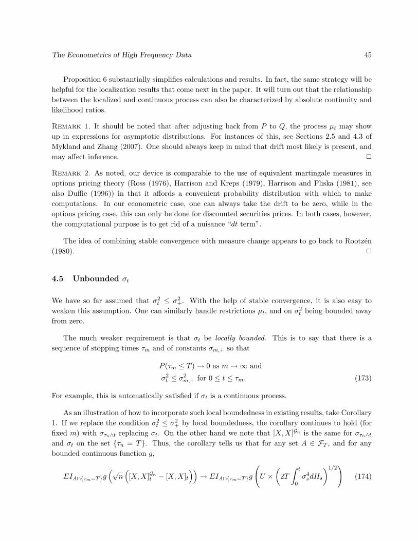
The Econometrics of High Frequency Data 45
Proposition 6 substantially simplifies calculations and results. In fact, the same strategy will behelpful for the localization results that come next in the paper. It will turn out that the relationshipbetween the localized and continuous process can also be characterized by absolute continuity andlikelihood ratios.
Remark 1. It should be noted that after adjusting back from P to Q, the process µt may showup in expressions for asymptotic distributions. For instances of this, see Sections 2.5 and 4.3 ofMykland and Zhang (2007). One should always keep in mind that drift most likely is present, andmay affect inference. 2
Remark 2. As noted, our device is comparable to the use of equivalent martingale measures inoptions pricing theory (Ross (1976), Harrison and Kreps (1979), Harrison and Pliska (1981), seealso Duffie (1996)) in that it affords a convenient probability distribution with which to makecomputations. In our econometric case, one can always take the drift to be zero, while in theoptions pricing case, this can only be done for discounted securities prices. In both cases, however,the computational purpose is to get rid of a nuisance “dt term”.
The idea of combining stable convergence with measure change appears to go back to Rootzen(1980). 2
4.5 Unbounded σt
We have so far assumed that σ2t ≤ σ2
+. With the help of stable convergence, it is also easy toweaken this assumption. One can similarly handle restrictions µt, and on σ2
t being bounded awayfrom zero.
The much weaker requirement is that σt be locally bounded. This is to say that there is asequence of stopping times τm and of constants σm,+ so that
P (τm ≤ T ) → 0 as m →∞ and
σ2t ≤ σ2
m,+ for 0 ≤ t ≤ τm. (173)
For example, this is automatically satisfied if σt is a continuous process.
As an illustration of how to incorporate such local boundedness in existing results, take Corollary1. If we replace the condition σ2
t ≤ σ2+ by local boundedness, the corollary continues to hold (for
fixed m) with στn∧t replacing σt. On the other hand we note that [X, X]Gn is the same for στn∧t
and σt on the set τn = T. Thus, the corollary tells us that for any set A ∈ FT , and for anybounded continuous function g,
EIA∩τm=Tg(√
n([X, X]Gn
t − [X, X]t))
→ EIA∩τm=Tg
(U ×
(2T
∫ t
0σ4
sdHs
)1/2)
(174)

The Econometrics of High Frequency Data 46
as n →∞ (and for fixed m), where U has the same meaning as in the corollary. Hence,
|EIAg(√
n([X, X]Gn
t − [X, X]t))
− EIAg
(U ×
(2T
∫ t
0σ4
sdHs
)1/2)|
≤ |EIA∩τm=Tg(√
n([X, X]Gn
t − [X, X]t))
− EIA∩τm=Tg
(U ×
(2T
∫ t
0σ4
sdHs
)1/2)|
+ 2 max |g(x)|P (τm 6= T )
→ 2 max |g(x)|P (τm 6= T ) (175)
as n →∞. By choosing m large, the right hand sice of this expression can be made as small as wewish. Hence, the left hand side actually converges to zero. We have shown:
Corollary 2. Theorem 7, Corollary 1, and Theorem 8 all remain true if the condition σ2t ≤ σ2
+ isreplaced by a requirement that σ2
t be locally bounded.
5 Microstructure
5.1 The Problem
The basic problem is that the semimartingale Xt is actually contaminated by noise. One observes
Yti = Xti + εi. (176)
We do not right now take a position on the structure of the εis.
The reason for going to this structure is that the convergence (consistency) predicted by The-orem 2 manifestly does not hold. To see this, in addition to G, we also use subgrids of the formHk = 0, tk, tK+k, t2K+k, .... This given rise to the Average Realized Voltatility (ARV)
ARV (Y,G,K) =1K
K∑k=1
[Y, Y ]Hk . (177)
Note that ARV (Y,G, 1) = [Y, Y ]G . If one believes Theorem 2, then the ARV (Y,G,K) should beclose for small K. In fact, the convergence in the theorem should be visible as K decreases to 1.Figure 1 looks at the ARV (Y,G,K) for Alcoa Aluminun (AA) for january 4, 2001. As can be seenin the figure, the actual data behaves quite differently from what the theory predicts. It followsthat the semimartingale assumption does not hold, and we have to move to a model like (176).
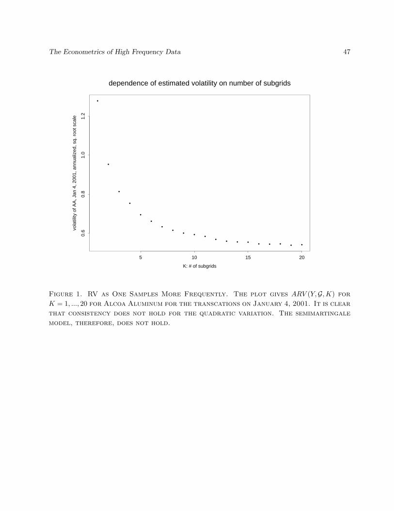
The Econometrics of High Frequency Data 47
•
•
•
•
••
••
• • •• • • • • • • • •
dependence of estimated volatility on number of subgrids
K: # of subgrids
vola
tility
of A
A, J
an 4
, 200
1, a
nnua
lized
, sq.
roo
t sca
le
5 10 15 20
0.6
0.8
1.0
1.2
Figure 1. RV as One Samples More Frequently. The plot gives ARV (Y,G,K) for
K = 1, ..., 20 for Alcoa Aluminum for the transcations on January 4, 2001. It is clear
that consistency does not hold for the quadratic variation. The semimartingale
model, therefore, does not hold.
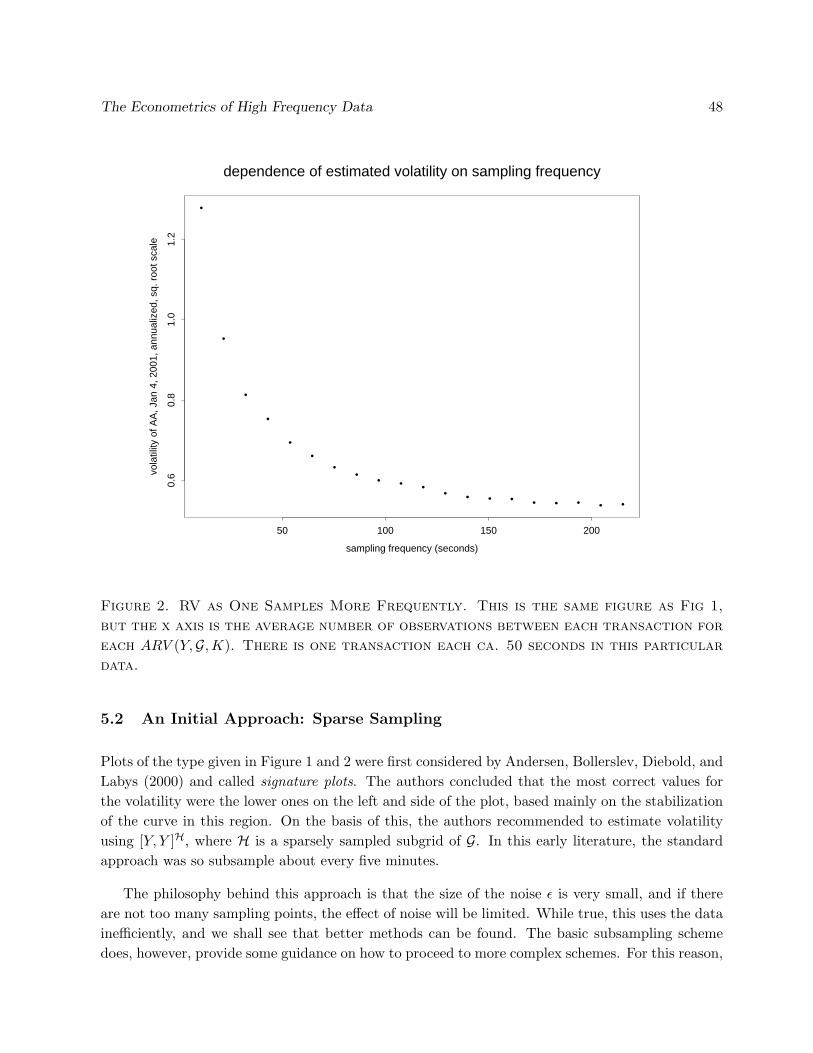
The Econometrics of High Frequency Data 48
•
•
•
•
••
••
• • •• • • • • • • • •
dependence of estimated volatility on sampling frequency
sampling frequency (seconds)
vola
tility
of A
A, J
an 4
, 200
1, a
nnua
lized
, sq.
roo
t sca
le
50 100 150 200
0.6
0.8
1.0
1.2
Figure 2. RV as One Samples More Frequently. This is the same figure as Fig 1,
but the x axis is the average number of observations between each transaction for
each ARV (Y,G,K). There is one transaction each ca. 50 seconds in this particular
data.
5.2 An Initial Approach: Sparse Sampling
Plots of the type given in Figure 1 and 2 were first considered by Andersen, Bollerslev, Diebold, andLabys (2000) and called signature plots. The authors concluded that the most correct values forthe volatility were the lower ones on the left and side of the plot, based mainly on the stabilizationof the curve in this region. On the basis of this, the authors recommended to estimate volatilityusing [Y, Y ]H, where H is a sparsely sampled subgrid of G. In this early literature, the standardapproach was so subsample about every five minutes.
The philosophy behind this approach is that the size of the noise ε is very small, and if thereare not too many sampling points, the effect of noise will be limited. While true, this uses the datainefficiently, and we shall see that better methods can be found. The basic subsampling schemedoes, however, provide some guidance on how to proceed to more complex schemes. For this reason,
The Econometrics of High Frequency Data 49
we shall analyze its properties.
The model used for most analysis is that εi is independent of X, and iid. One can still, however,proceed under weaker conditions. For example, if the εi have serial dependence, a similar analysiswill go through.
The basic decomposition is
[Y, Y ]H = [X, X]H + [ε, ε]H + 2[X, ε]H, (178)
where the cross term is usually (but not always) ignorable. Thus, if the ε’s are independent of X,and E(ε) = 0, we get
E([Y, Y ]H|X process) = [X, X]H + E[ε, ε]H. (179)
If the ε are identically distributed, then
E[ε, ε]H = nsparseE(εK − ε0)2, (180)
where nsparse = number of points in H,−1. Smaller nsparse gives smaller bias, but bigger variance.
At this point, if you would like to follow this line of development, please consult the discussionin Section 2 in (Zhang, Mykland, and Aıt-Sahalia (2005)). This shows that there is an opti-mal subsampling frequency, given by equation (31) (p 1399) in the paper. A similar analysis forARV (Y,G,K) is carried out in Section 3.1-3.3 of the paper.
5.3 Two Scales Realized Volatility (TSRV)
To get a consistent estimator, we go to the two scales realized volatility (TSRV). The TRSV isdefined as follows.
[X, X](tsrv)
T = anARV (Y,G,K)− bnARV (Y,G, J) (181)
where we shall shortly fix an and bn. It will turn out to be meaningful to use
bn = an ×nK
nJ, (182)
where nK = (n−K +1)/K. For asymptotic purposes, we can take an = 1, but more generally willassume that an → 1 as n →∞.
This estimator is discussed in Section 4 in Zhang, Mykland, and Aıt-Sahalia (2005), thoughonly in the case where J = 1. In the more general case, J is not necessarily 1, but J << K.
One can prove under weak assumptions, that
n−J∑i=0
(Xti+j −Xti)(εti+j − εti) = Op(J1/2).

The Econometrics of High Frequency Data 50
This important because it gives rise to the sum of squares decomposition
[Y, Y ](J)T = [X, X](J)
T + [ε, ε](J)T + Op(J−1/2),
Thus, if we look at linear combinations of the form (181), one obtains, for an = 1,
[X, X](tsrv)
T = [X, X](K)T − nK
nJ[X, X](J)
T︸ ︷︷ ︸signal term
+ [ε, ε](K)T − nK
nJ[ε, ε](J)
T︸ ︷︷ ︸noise term
+ Op(K−1/2), (183)
so long as1 ≤ J ≤ K and K = o(n). (184)
The noise term behaves as follows:
[ε, ε](J)T =
1J
n∑i=0
c(J)i ε2ti −
2J
n−J∑i=0
εtiεti+J , (185)
where c(J)i = 2 for J ≤ i ≤ n− J , and = 1 for other i. By construction∑
i
c(J)i = 2JnJ , (186)
So that
noise term ≈ − 2K
n−K∑i=0
εtiεti+K +nK
nJ
2J
n−J∑i=0
εtiεti+J (187)
so that (1) the ε2 terms have been removed, and (2) the estimator is unbiased if J is chosen to bebigger than the range of dependence.
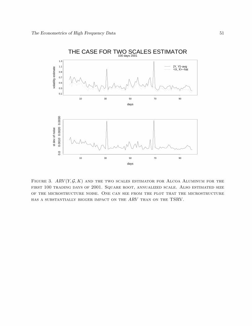
The Econometrics of High Frequency Data 51
days
vola
tility
est
imat
e
0.1
0.3
0.5
0.7
0.9
1.1
1.3
10 30 50 70 90
[Y, Y]−avg<X, X>−hat
days
st d
ev o
f noi
se
0.0
0.00
100.
0020
0.00
30
10 30 50 70 90
THE CASE FOR TWO SCALES ESTIMATOR100 days 2001
Figure 3. ARV (Y,G,K) and the two scales estimator for Alcoa Aluminum for the
first 100 trading days of 2001. Square root, annualized scale. Also estimated size
of the microstructure noise. One can see from the plot that the microstructure
has a substantially bigger impact on the ARV than on the TSRV.

The Econometrics of High Frequency Data 52
• •
•
•
•••
••
•
•
•• •
•
•
•
•
••
•
•
••
••
•
•
•
•
•
•
•
••
••
••
•
•
•
••
•
•
•
••
•
••
••
•
•
•
•
•
••
•
•••
•
••
•
••
•
••
•
•••
• •
•
••
••• •• •
•••
•
••
•
•
•
••
two scales volatility
st d
ev e
rror
0.2 0.3 0.4 0.5
0.00
20.
004
0.00
60.
008
ERROR PROPORTIONAL TO VOLATILITY?
Figure 4. Data as in Fig. 3. Here size of microstructure noise plotted vs. TSRV.
The figure suggests that the size of the microstructure is largely unaffected by
the volatility.
5.4 Asymptotics for the TSRV
If the noise is assumed to be independent of the X process, one can deal separately with the signaland noise terms in (183). The signal term is analyzed with the kind of technique developed Sections3-4 above. The precise derivation is given in Section 3.4 (p. 1400-1401) and Appendix A.3 (p. 1410-1411) of Zhang, Mykland, and Aıt-Sahalia (2005). Meanwhile, the noise term (187) is a U-statisticwhich can be handled with methods from discrete process limit theory, based either on martingalesor mixing, using the limit theory in Hall and Heyde (1980) (see, in particular, ibid., Theorem 3.2(p. 58-59)). For concrete implementation, see Zhang, Mykland, and Aıt-Sahalia (2005) for the caseof iid noise. By combining the two sources of error in (183), the optimal rate of convergence of theTSRV to the true integrated volatility is Op(n−1/6), and the limit is, again, of mixed normal type.
The Econometrics of High Frequency Data 53
5.5 The emerging literature on estimation of volatility under microstructure
. This estimation problem has by now become somewhat of an industry. The following approachesare now in the process of becoming available:
• Extensions of the two scales approach. Zhang (2006) studies a multi scale realized volatility(MSRV), and obtains that the estimator of integrated volatility converges at the rate ofOp(n−1/4). This rate is optimal, as it also comes up in the case where σt is constant and thenoise is normal, which is a parametric problem. Also, the conditions on the noise structurein the TSRV has been weakened. Aıt-Sahalia, Mykland, and Zhang (2008) studies noise thatis internally dependent but independent of the signal, and Li and Mykland (2007) discussesa formulation where where the noise can depend on the process X.
• An approach based on autocovariances. Often called the “kernel” approach. This work hasbeen pioneered by Barndorff-Nielsen, Hansen, Lunde, and Shephard (2008). We refer to thispaper for further discussion.
• Preaveraging. The idea here is to try to reduce the noise by averaging observations beforecomputing volatilities. The two main papers for the moment are Jacod, Li, Mykland, Podol-skij, and Vetter (2009) and Podolskij and Vetter (2009).
• Likelihood based methods. There are here two approaches under development. On the onehand, Xiu (2009) uses the likelihood function for constant σ and normal noise as a quasi-likelihood to estimate [X, X]. On the other hand, Mykland and Zhang (2007) show that insufficiently small neighboorhoods of observations, one can act as if σt really is constant. Wereturn to a discussion of this in Section 6.
To first order, all of these estimators do similar things. The main difference between them seemsto be the handling of end effects. This topic will, no doubt, be the subject of future research.
5.6 A wider look at subsampling and averaging
We have seen above that subsampling and averaging can help with several problems.
1. It is a first order remedy for microstructure.
2. If an estimator [X, X] is based on the noise being an independent series, one can amelioratethe effects of actual dependence by subsampling every J ’th observation, and then averageacross the J resulting estimators. We have explicitly described this for the TSRV, but thesame rationale can be used to subsample and then average any of the estimators mentionedin Section 5.5.
The Econometrics of High Frequency Data 54
3. A further use of subsampling is that it seems in some instances to regularize time. This isfurther discussed in Section 7.2.
6 Methods based on Contiguity
We have seen in Section 4.4 that measure changes can be a powerful tool in high frequency dataproblems. We here pursue this matter further, by considering measure changes that are asymptot-ically absolutely continuous. This is closely related to the concept of contiguity, which is discussedfurther in Section 6.1. This first section mainly abstracts the results in Mykland and Zhang (2007),which should be consulted for details and proofs. The later sections is new material.
6.1 Block Discretization
In addition to the grid Gn = 0 = tn,0 < tn,1 < ... < tn,n = T, which we again take to beindependent of the underlying process to be observed, we consider a subgrid
Hn = 0 = τn,0 < τn,1 < ... < τn,Kn = T ⊆ Gn. (188)
We shall now define a new measure, on the observations Xtn,j only, for which the volatility isconstant on each of the Kn blocks (τn,i−1, τn,i]. Secifically, define the approximate measure, calledQn, given by X0 = x0 and
for each i = 1,Kn : ∆Xtj+1 = στn,i−1∆WQtj+1
for tn,j+1 ∈ (τn,i−1, τn,i]. (189)
Formally, we define the approximation recursively:
Definition 10. (Block approximation). Define the probability Qn recursively by:(i) U0 has same distribution under Qn as under P ;(ii) The conditional Qn-distribution of U
(1)tn,j+1
given U0, ..., Utn,j is given by (189), where ∆WQtj+1
is conditionally normal N(0,∆tj+1), and(iii) The conditional P ∗
n-distribution of U(2)tn,j+1
given U0, ..., Utn,j , U(1)tn,j+1
is the same as under P .
Denote by Mn,i = #tn,j ∈ (τn,i−1, τn,i] We shall require that that maxi Mn,i = O(1) as n →∞, from which it follows that Kn is of exact order O(n). To measure the extent to which we holdthe volatility constant, we define the following “Asymptotic Decoupling Delay” (ADD) by
K(t) = limn→∞
∑i
∑tn,j∈(τn,i−1,τn,i]∩[0,t]
(tn,j − τn,i−1), (190)
provided the limit exists. In the case of equidistant observations and equally sized blocks of M
observations, the ADD takes the form K(t) = 12(M − 1)t.

The Econometrics of High Frequency Data 55
In is shown in (Theorems 1 and 3 in) Mykland and Zhang (2007) that, subject to regularityconditions, P and Pn are mutually absolutely continuous on the σ-field Xn,n generated by Utn,j ,j = 0, ..., n. Furthermore, let (dP ∗/dP ∗
n)(Ut0 , ..., Utn,j , ..., Utn,n) be the likelihood ratio (Radon-Nikodym derivative) on Xn,n. Then,
dP
dQn(Ut0 , ..., Utn,j , ..., Utn,n) L→ expΓ1/2N(0, 1)− 1
2Γ (191)
stably in law, under Qn, as n →∞. The asymptotic variance is given by Γ = Γ0 + Γ1, where
Γ0 =38
∫ T
0
(1σ2
t
d
dt[σ2,W ]t
)2
dt =32
∫ T
0
(1σt
d
dt[σ,W ]t
)2
dt, and
Γ1 =12
∫ T
0
1σ4
t
(d
dt[σ2, σ2]t
)dK(t) = 2
∫ T
0
1σ2
t
(d
dt[σ, σ]t
)dK(t) (192)
Hence, Γ0 is related to the leverage effect, while Γ1 is related to the volatility of volatility.
The important consequence of this result is that that P and the approximation Qn are contiguousin the sense of Hajek and Sidak (1967) (Chapter VI), LeCam (1986), LeCam and Yang (1986), andJacod and Shiryaev (2003) (Chapter IV). This is to say that for a sequence An of sets, P (An) → 0if and only if Qn(An) → 0. This follows from (191) since dP/dQn is uniformly integrable underQn (since the sequence dP/dQn is nonnegative, also the limit integrates to one under Qn). In itfollows that consistency and orders of convergence are maintained from one measure to the other.In particular, a martingale Zn is Op(1) under P if and only if it has the same order of convergenceunder Qn. Hence consistency and order of convergence are maintained from one measure to theother. The result in the cited paper also covers the multivariate case. Also consult ibid., Section3.3, for connections to Hermite polynomials. Finally note that contiguity also holds if the sequencedPdQn
is tight, which requires even weaker conditions. (For example, K need only exist throughsubsequences, which is assured by under weak conditions by Helly’s Theorem, (see, for example, p.336 in Billingsley (1995)).
The good news: This means that one can construct estimators as if σ2t is locally constant. If
the resulting estimator θn is such that nα(θn − θ) = Op(1) under Qn (where local constancy issatisfied), then nα(θn − θ) = Op(1) also under P . In other words, the change from P to Qn hasmuch the same simplifying function as the measure change in Section 4.4.
Remark 3. The (potentially) bad news: This change of measure is not completely innocuous. Asequence Zn of martingales may not have exactly the same limit distribution under P and Qn.The reason is that the Qn martingale part of log dP/dQn may have nonzero asymptotic covariationwith Zn. This is the same phenomenon which occurs (in a different context) in Section 4.3.2. Anadjustment then has to be carried out along the lines of “LeCam’s Third Lemma” (Hajek and Sidak(1967), Chapter VI.1.4., p. 208). We refer to Section 2.4 and 3.4 of Mykland and Zhang (2007)for the methodology for adjusting the limit distribution. Ibid., Section 4.3, provides an examplewhere such an adjustment actually has to be made. Other parts of Section 4 of the paper providesexamples of how the methodology can be used, and where adjustment is not necessary. 2
The Econometrics of High Frequency Data 56
The approximation above depends on the following Ito process structure on σ:
dσt = σtdt + ftdWt + gtdBt. (193)
where B a Brownian motion independent of W . (It is an open question what happens in, say,the long range dependent case). We also require inf0≤t≤T σ2 > 0. Note that in the representation(193), (192) becomes
Γ0 =32
∫ T
0
(ft
σt
)2
dt and Γ1 = 2∫ T
0
(f2
t + g2t
σ2t
)dt (194)
Example 10. In the case of a Heston model (Section 2.2.3), we obtain that
Γ0 =38(ργ)2
∫ T
0σ−2
t dt and Γ1 =14γ2(M − 1)
∫ T
0σ−2
t dt. (195)
Remark 4. (One step discretization). Let P ∗n be the measure Qn which arises when the block
length is M = 1. Observe that even with this one-step discretization, dP/dP ∗n does not necessarily
converge to unity. In this case, Γ1 = 0, but Γ0 does not vanish when there is leverage effect.2
6.2 Moving windows
The paper so far has considered chopping n data up into non-overlapping windows of size M each.We here show by example that the methodology can be adapted to the moving window case. Weconsider the estimation of θ =
∫ T0 |σt|pdt, as in Section 4.1 of Mykland and Zhang (2007). It should
be noted that the moving window is close to the concept of a moving kernel, and this may be apromising avenue of further investigation. See, in particular, Linton (2007).
We use block length M , and we use for simplicity
σ2τn,i
=1
∆tnMn
∑tn,j∈(τn,i,τn,i+1]
(∆Xtn,j+1)2, (196)
as estimator of σ2τn,i
. The moving window estimate of θ is now
θMWn = (∆t)
n−M∑i=0
|σtn,i |r.
It is easy to see that
θMWn =
1M
M∑m=1
θn,m + Op(n−1),
where θn,m is the non-overlapping block estimator, with block number one starting at tn,m. Inview of this representation, it is once again clear from sufficiency considerations that the moving
The Econometrics of High Frequency Data 57
window estimator will have an asymptotic variance which is smaller (or, at least, no larger) thanthe estimator based on non-overlapping blocks. We now carry out the precise asymptotic analysis.
To analyze this estimator, let M > M , and let An = i = 0, ..., n − M : [tn,i, tn,i+M ] ⊆[kM, (k + 1)M] for some k, with Bn = 0, ..., n−M −An. Write
n1/2(θMWn − θ) = n1/2∆t
∑k
∑i:[tn,i,tn,i+M ]⊆[kM/n,(k+1)M/n]
(|σtn,i |r − |σtkM |r)
+ n1/2∆t∑i∈Bn
(|σtn,i |r − |σtn,i |r) + Op(n−1/2). (197)
Now apply our methodology from Section 6.1, with block size M, to the first term in (197). Underthis block approximation, the inner sum in the first term is based on conditionally i.i.d. observations,in fact, for [tn,i, tn,i+M ] ⊆ [kM/n, (k + 1)M/n], σ2
tn,i= σ2
kM/nSi, in law, where
Si = M−1i+M−1∑
j=i
U2j , U0, U1, U2, ... iid standard normal. (198)
As in Section 4.1 of Mykland and Zhang (2007), there is no adjustment (a la Remark 3) dueto covariation with the asymptotic likelihood ratios, and so the first term in (197) converges stablyto a mixed normal with random variance as the limit of n∆t2n
∑k |σ|rkM/nVar
(c−1M,r
∑M−Mi=0 Sr/2
i
),
which is
Tc−2M,r
1M
Var
(M−M∑i=0
Sr/2i
)∫ T
0|σ|rtdt. (199)
Similarly, one can apply the same technique to the second term in (197), but now with the k’thblock (k ≥ 2) starting at kM−M . This analysis yields that the second term is also asymptoticallymixed normal, but with a variance what is of order op(1) as M→∞. (In other words, once again,first send n to infinity, and then, afterwards, do the same to M). This yields that, overall, and inthe sense of stable convergence,
n1/2(θMWn − θ) L→ N (0, 1)×
(c−2M,rαM,rT
∫ T
0|σ|rtdt
)1/2
, (200)
where, from (199), αM,r = limM→∞Var(∑M−M
i=0 Sr/2i
)/M, i.e.,
αM,r = Var(Sr/20 ) + 2
M−1∑i=1
Cov(Sr/20 ,Sr/2
i ),
where the Si are given in (198).
The Econometrics of High Frequency Data 58
6.3 Multivariate and Asynchronous data
The results discussed in Section 6.1 also apply to vector processes (see Mykland and Zhang (2007)for details). Also, for purposes of analysis, asynchronous data does not pose any conceptual diffi-culty when applying the results. One includes all observation times when computing the likelihoodratios in the contiguity theorems. It does not matter that some components of the vector are notobserved at all these times. In a sense, they are just treated as missing data. Just as in the caseof irregular times for scalar processes, this does not necessarily mean that it is straightforward towrite down sensible estimators.
For example, consider a bivariate process (X(1)t , X
(2)t ). If process (X(r)
t ) is observed at times :
G(r)n = 0 ≤ t
(r)n,0 < t
(r)n,1 < ... < t(r)n,n1
≤ T, (201)
one would normally use the grid Gn = G(1)n ∪G(2)
n ∪ 0, T to compute the likelihood ratio dP/dQn.
To focus the mind with an example, consider the estimation of covariation under asynchronousdata. It is shown in Mykland (2006) that the Hayashi-Yoshida estimator (Hayashi and Yoshida(2005)) can be seen as a nonparametric maximum likelihood estimator (MLE). We shall here seethat blocking induces an additional class of local likelihood based MLEs. The difference betweenthe former and the latter depends on the continuity assumptions made on the volatility process,and is a little like the difference between the Kaplan-Meier (Kaplan and Meier (1958)) and Nelson-Aalen (Nelson (1969), Aalen (1976, 1978)) estimators in survival analysis. (Note that the varianceestimate for the Haysahi-Yoshida estimator from Section 5.3 of Mykland (2006) obviously alsoremains valid in the setting of this paper).
For simplicity, work with a bivariate process, and let the grid Gn be given by (201). For now,let the block dividers τ be any subset of Gn. Under the approximate measure Qn, note that for
τn,i−1 ≤ t(1)n,j−1 < t
(1)n,j ≤ τn,i and τn,i−1 ≤ t
(2)k−1 < t
(2)k ≤ τn,i (202)
the set of returns X(1)
t(1)n,j
− X(1)
t(1)n,j−1
and X(2)
t(2)n,k
− X(2)
t(2)n,k−1
are conditionally jointly normal with mean
zero and covariances
CovQn(X(r)
t(r)n,j
−X(r)
t(r)n,j−1
,X(s)
t(s)n,k
−X(s)
t(s)n,k−1
) | Fτn,i−1) = (ζτn,i−1)r,sd(t(r)n,j−1, t
(r)n,j) ∩ (t(s)n,k−1, t
(s)n,k) (203)
where d is length (Lebesgue measure). Set κr,s,j,k = ζd(t(r)n,j−1, t(r)n,j) ∩ (t(s)n,k−1, t
(s)n,k). The Qn log
likelihood ratio based on observations fully in block (τn,i−1, τn,i] is therefore given as
`(ζ) = −12
ln det(κ)− 12
∑r,s,j,k
κr,s;j,k(X(r)
t(r)n,j
−X(r)
t(r)n,j−1
)(X(s)
t(s)n,k
−X(s)
t(s)n,k−1
)− Ni
2ln(2π), (204)
where κr,s;j,k are the elements of the matrix inverse of (κr,s;j,k), and Ni is a measure of blocksample size. The sum in (j, k) is over all intersections (t(r)n,j−1, t
(r)n,j) ∩ (t(s)n,k−1, t
(s)n,k) with positive
The Econometrics of High Frequency Data 59
length satisfying (202). Call the number of such terms
m(r,s)n,i = # nonempty intersections (t(r)n,j−1, t
(r)n,j) ∩ (t(s)n,k−1, t
(s)n,k) satisfying (202) . (205)
The “parameter” ζ corresponds to ζτn,i−1 . The block MLE is thus given as
ζ(r,s)τn,i−1
=1
m(r,s)n,i
∑j,k
(X(r)
t(r)n,j
−X(r)
t(r)n,j−1
)(X(s)
t(s)n,k
−X(s)
t(s)n,k−1
)
d(t(r)n,j−1, t(r)n,j) ∩ (t(s)n,k−1, t
(s)n,k)
(206)
where the sum is over j, k satisfying (202) for which the denominator in the summand is nonzero.The overall estimate of covariation is thus
〈X(r), X(s)〉T =∑
i
ζ(r,s)τn,i−1
(τn,i − τn,i−1). (207)
We suppose, of course, that each block is large enough for m(r,s)n,i to be always greater than zero.
Under Qn, EQn(ζτn,i−1 |Fτn,i−1) = ζτn,i−1 , and
VarQn(ζ(r,s)τn,i−1
|Fτn,i−1) =
(1
m(r,s)n,i
)2ζ(r,r)
τn,i−1ζ(s,s)τn,i−1
∑j,k
(t(r)n,j − t(r)n,j−1)(t
(s)n,k − t
(s)n,k−1)
d(t(r)n,j−1, t(r)n,j) ∩ (t(s)n,k−1, t
(s)n,k)2
+ (ζ(r,s)τn,i−1
)2∑
j1,j2,k1,k2
d(t(r)n,j1−1, t(r)n,j1
) ∩ (t(s)n,k2−1, t(s)n,k2
)d(t(r)n,j2−1, t(r)n,j2
) ∩ (t(s)n,k1−1, t(s)n,k1
)
d(t(r)n,j1−1, t(r)n,j1
) ∩ (t(s)n,k1−1, t(s)n,k1
)d(t(r)n,j2−1, t(r)n,j2
) ∩ (t(s)n,k2−1, t(s)n,k2
)
,
(208)
The first sum is over the same (j, k) as in (206), and the second sum is over all j1, j2, k1, k2 satisfying(202), again for which the denominator in the summand is nonzero.
It is therefore easy to see that subject to conditions on the observation times t(r)n,i and t
(s)n,i,
n1/2( 〈X(r), X(s)〉T − 〈X(r), X(s)〉T ) converges stably (under Qn), to a mixed normal distributionwith variance as the limit of
n∑
i
VarQn(ζ(r,s)τn,i−1
|Fτn,i−1)(τn,i − τn,i−1)2. (209)
It is straightforward to see that there is no adjustment from Qn to P . A formal asymptotic analysiswould be tedious, and has therefore been omitted. In any case, to estimate the asymptotic variance,one would use (208)-(209), with ζτn,i−1 replacing ζτn,i−1 in (208).
Remark 5. An important difference from the Hayashi-Yoshida estimator is that (206) dependson the observation times. This is in many instances undesirable, and the choice of estimator willdepend on the degree to which these times are trusted. The Hayashi-Yoshida estimator is alsoaesthetically more pleasing. We note, however, that from likelihood considerations, the estimator
The Econometrics of High Frequency Data 60
(206) will have an asymptotic variance which, as the block size tends to infinity, converges to alimit which corresponds to the efficient minimum for constant volatility matrix.
This phenomenon can be best illustrated for a scalar process (so there is no asynchronicity). Inthis case, our estimator (206) of 〈X, X〉T becomes (for block size M fixed)
〈X, X〉T =∑
i
(τn,i − τn,i−1)1M
∑j: τn,i−1<tn,j≤τn,i
∆X2tn,j
∆tn,j. (210)
It is easy to see, by the methods in this paper, or directly, that for this estimator, the asymptoticvariance is 2T
∫ T0 σ4
t dt, while for the standard realized volatility, the corresponding expression is2T∫ T0 σ4
t H′(t)dt, where H(t) is the asymptotic quadratic variation of time (142). It is always the
case that H ′(t) ≥ 1, and when observations are sufficiently irregular (under, say, Poisson sampling,the inequality is strict, cf. Section 7.2 below. Thus, (210) is more efficient than regular realizedvolatility, but since the times can in many cases not be trusted, the realized volatility remains amain tool for estimating volatility. 2
6.4 More complicated data generating mechanisms
6.4.1 Jumps
We only consider the case of finitely many jumps (compound Poisson processes, and similar). Theconceptually simplest approach is to remove these jumps using the kind of procedure described inMancini (2001) and Lee and Mykland (2006). The procedure will detect all intervals (tn,j−1, tn,j ],with probability tending to one (exponentially fast) as n →∞. If one simply removes the detectedintervals from the analysis, it is easy to see that our asymptotic results go through unchanged.
The case of infinitely many jumps is more complicated, and beyond the scope of this paper.
Note that there is a range of approaches for estimating the continuous part of volatility insuch data. Methods include bi- and multi-power (Barndorff-Nielsen and Shephard (2004b). Otherdevices are considered by Aıt-Sahalia (2004), and Aıt-Sahalia and Jacod (2007). One can use ourmethod of analysis for all of these approaches.
6.4.2 Microstructure noise
The presence of noise does not alter the analysis in any major way. Suppose one observes
Ytn,j = Xtn,j + εn,j (211)
where the εn,j ’s are independent of the (Xt) process. The latter still follows (97). We take theσ-field Xn,n to be generated by Xtn,j , εn,j , 0 ≤ j ≤ n. Suppose that P1 and P2 are two measures

The Econometrics of High Frequency Data 61
on Xn,n for which: (1) the variables εn,j , 0 ≤ j ≤ n are independent of Xn,j , 0 ≤ j ≤ n,and (2) the variables εn,j , 0 ≤ j ≤ n have the same distribution under P1 and P2. Then, fromstandard results in measure theory,
dP2
dP1((Xn,j , εn,j), 0 ≤ j ≤ n) =
dP2
dP1(Xn,j , 0 ≤ j ≤ n) (212)
The results in our theorems are therefore unchanged in the case of microstructure noise (unless onealso wants to change the probability distribution of the noise). We note that this remains the caseirrespective of the internal dependence structure of the noise.
The key observation which leads to this easy extension is that it is not required for our resultsto work that the observables Ytn,j generate the σ-field Xn,n. It is only required that the observablesbe measurable with respect to this σ-field. The same principle was invoked in Section 6.3.
The extension does not, obviously, solve all problems relating to microstructure noise, since thistype of data generating mechanism is best treated with an asymptotics where M →∞ as n →∞.This is currently under investigation.
7 Irregularly spaced data
7.1 A second block approximation.
The approximation in Section 6.1 reduces the problem (in each block) to a case of independent (butnot identically distributed) increments. Can we do better than this, and go to iid observations?We here give a criterion for this to be the case.
Consider yet another approximate probability measure Rn, under which X0 = x0, and
for each i = 1, ...,Kn : ∆Xtj+1 = στn,i−1(∆τi
∆tj+1Mi)1/2∆W ∗
tj+1for tn,j+1 ∈ (τn,i−1, τn,i] (213)
Formally, we define the approximation as follows.
Definition 11. Rn is defined as Qn in Definition 10, but with (213) replacing (189).
The crucial fact will be that under Rn, the observables ∆Xtj+1 are conditionally iid N(0, ζτn,i−1∆τi/Mi)for tn,j+1 ∈ (τn,i−1, τn,i].
So that the following can be used together with the results in Mykland and Zhang (2007), wewill in the following let the process X be multivariate, and we make the following assumption
Assumption 2. (Structure of the instantaneous volatility). We assume that the matrix process σt
is itself an Ito processes, and that if λ(p)t is the smallest eigenvalue of σt, then inft λ
(p)t > 0 a.s.

The Econometrics of High Frequency Data 62
The contiguity question is then addressed as follows. Let P ∗n be the measure from Remark 4
(corresponding to block length M = 1). Recall that
logdRn
dP= log
dRn
dQn+ log
dQn
dP ∗n
+ logdP ∗
n
dP(214)
Define
Bn,j =
(∆tn,j+1
(∆τn,i
Mi
)−1
− 1
)(215)
Theorem 11. (Asymptotic relationship between P ∗n , Qn and Rn). Assume the conditions of The-
orem 4 in Mykland and Zhang (2007), and let Z(1)n and M
(1)n be as in that theorem (see (231) and
(234) in Section 7.3). Assume that the following limits exist:
Γ2 =p
2lim
n→∞
∑j
B2n,j and Γ3 =
p
2lim
n→∞
∑j
log(1 + Bn,j). (216)
Set
Z(2)n =
12
∑i
∑tn,j∈(τn,i−1,τn,i]
∆XTtn,j
((σσT )−1
τn,i−1)∆Xtn,j
(∆t−1
n,j+1 −(
∆τn,i
Mi
)−1)
, (217)
and let M(2)n be the end point of the martingale part of Z
(2)n (see (232) and (234) in Section 7.3 for
the explicit formula). Then, as n →∞, (M (1)n ,M
(2)n ) converges stably in law under P ∗ to a normal
distribution with mean zero and diagonal variance matrix with diagonal elements Γ1 and Γ2. Also,under P ∗,
logdRn
dQn= M (2)
n + Γ3 + op(1). (218)
The theorem can be viewed from the angle of contiguity:
Corollary 3. Under regularity conditions, the following statements are equivalent, as n →∞:(i) Rn is contiguous to P .(ii) Rn is contiguous to Qn.(iii) The following relationship holds:
Γ3 = −12Γ2. (219)
As we shall see, the requirement (219) is a substantial restriction. Corollary 3 says that unlikethe case of Qn, inference under Rn may not give rise to desired results. Part of the probabilitymass under Qn (and hence P ∗) is not preserved under Rn.
To understand the requirement (219), note that
p
2
∑j
log(1 + Bn,j) = −p
4
∑j
B2n,j +
p
6
∑j
B3n,j − ... (220)

The Econometrics of High Frequency Data 63
since∑
j Bn,j = 0. Hence, (219) will, for example, be satisfied if maxj |Bn,j | → 0 as n → ∞. Onesuch example is
tn,j = f(j/n) and f is continuously differentiable. (221)
However, (221) will not hold in more general settings, as we shall see from the following examples.
Example 11. (Poisson sampling.) Suppose that the sampling time points follow a Poissonprocess with parameter λ. If one conditions on the number of sampling points n, these points behavelike the order statistics of n uniformly distributed random variables (see, for example, Chapter 2.3in Ross (1996)). Consider the case where Mi = M for all but (possibly) the last interval inHn. In this case, Kn is the smallest integer larger than or equal to n/M . Let Yi be the M -tuple(Bj , τi−1 ≤ tj < τi).
We now obtain, by passing between the conditional and unconditional, that Y1, ..., YKn−1 are iid,and the distribution can be described by
Y1 = M(U(1), U(2) − U(1), ..., U(M−1) − U(M−2), 1− U(M−1))− 1, (222)
where U(1), ..., U(M−1) is the order statistic of M − 1 independent uniform random variables on(0, 1). It follows that ∑
j
B2n,j =
n
M(M2EU2
(1) − 1) + op(n)
∑j
log(1 + Bn,j) =n
ME log(MU(1)) + op(n) (223)
since EU2(1) = 2/(M+1)(M+2). Hence, both Γ2 and Γ3 are infinite. The contiguity between Rn and
the other probabilities fails. On the other hand all our assumptions up to Section ?? are satisfied,and so P , P ∗
n and Qn are all contiguous. The AQVT (equation (142)) is given by H(t) = 2t . Also,if the block size is constant (size M), the ADD is K(t) = (M − 1)t .
Example 12. (Systematic irregularity.) Let ε be a small positive number, and let ∆tn,j =(1 + ε)T/n for odd j and ∆tn,j = (1 − ε)T/n for even j (with ∆tn,j = T/n for odd n). Again,all our assumptions up to Section 6 are satisfied. The AQVT is given by H(t) = t(1 + ε2). If wesuppose that all Mi = 2, the ADD becomes K(t) = t. On the other hand, Bn,j = ±ε, so that, again,both Γ2 and Γ3 are infinite. The contiguity between Rn and the other probabilities thus fails in thesame radical fashion as in the case of Poisson sampling.
7.2 Irregular Spacing and Subsampling
We here return to a more direct study of the effect of irregular spacings. We put ourselves in thesituation from Section 4.3.1, where observation times are independent of the process. As stated
The Econometrics of High Frequency Data 64
in equation (160), the limit law for the realized volatility (for√
n([X, X]Gn
t − [X, X]t)) is mixed
normal with (random) variance
2T
∫ t
0σ4
sdHs, (224)
where H is the asymptotic quadratic variation of time (AQVT). When observations are equidistant,H ′(t) ≡ 1. From the preceeding section, we also know that if times are on the form (221), theasymptotic variance is unaffected. It is worth elaborating on this in direct computation. Set
F (t) = limn→∞
1n
#tn,i+1 ≤ t (225)
this quantity exists, if necessary by going through subsequences (Helly’s Theorem, see, for example,p. 336 in Billingsley (1995)). Set
un,i = F (tn,i). (226)
Asymptotically, the un,i are equispaced:
1n
#un,i+1 ≤ t =1n
#tn,i+1 ≤ F (−1)(t) → F (F (−1)(t)) = t (227)
Inference is invariant to this transformation: Observing the process Xt at times tn,i is the sameas observing the process Yt = XF (−1)(t) at times un,i. If we set U = un,j , j = 0, ..., n, then[X, X]GT = [Y, Y ]UT . Also, in the limit, [X, X]T = [Y, Y ]T . Finally, the asymptotic distribution thesame in these two cases
If the un,i have AQVT U(t), the mixed normal variance transforms
2T
∫ T
0H ′(u)(〈X, X〉′t)2dt = 2
∫ 1
0U ′(u)(〈Y, Y 〉′t)2dt. (228)
The transformation (226) regularizes spacing. It means that without loss of generality, one cantake T = 1, F ′ = 1 and and U = H. Also, the transformation (226) regularizes spacing defined by(221), and in this case, U ′(t) ≡ 1.
Example 13. On the other hand, it is clear from Example 11 that it is possible for U ′(t) to takeother values than 1. The example shows that for Poisson distributed observation times, H ′ = U ′ ≡ 2,while, indeed F ′(t) ≡ 1/T .
The general situation can be expressed as follows:
Proposition 7. Assume that F exists and is monotonely increasing. Also assume that H exists.Then U exists. For all s ≤ t, U(t) − U(s) ≥ t − s. In particular, if U ′(t) exists, then U ′(t) ≥ 1.The following statements are equivalent:(i) U(1) = 1(ii) U ′ ≡ 1(iii)
∑nj=0
(un,j+1 − un,j − 1
n
)2 = op(n−1)

The Econometrics of High Frequency Data 65
Proof of Proposition 7. The first statement uses a standard property of the variance: if ∆tn,j+1 =tn,j+1 − tn,j , and ∆n = T/n, then
n
T
∑tn,j+1≤t
(∆tn,j+1)2 =n
T
∑tn,j+1≤t
(∆tn,j+1 −∆n)2 +n
T#tn,i+1 ≤ t(∆n)2
≥ n
T#tn,i+1 ≤ t(∆n)2
By taking limits as n →∞ under F ′(t) ≡ 1/T , we get that H(t)−H(s) ≥ t− s. In particular, thesame will be true for U .
The equivalence between (i) and (iii) follows from the proof of Lemma 2 (p. 1029) in Zhang(2006). (The original lemma uses slightly different assumptions).
The implication of the proposition is that under the scenario U(1) = 1, observation times are“almost” equidistant. In particular, subsampling does not change the structure of the spacings.On the other hand, when U(1) > 1, there is scope for subsampling to regularize the times.
Example 14. Suppose that the times are Poisson distributed. Instead of picking every observation,we now pick every M ’th observation. By the same methods as in Example 11, we obtain that
U(t) =M + 1
Mt. (229)
Hence the sparser the subsampling, the more regular the times will be. This is an additional featureof subsampling that remains to be exploited.
7.3 Proof of Theorem 11
We begin by describing the relationship between Rn and P ∗n . In analogy with Proposition 2 of
Mykland and Zhang (2007), we obtain that
Lemma 2.
logdRn
dP ∗n
(Ut0 , ..., Utn,j , ..., Utn,n)
=∑
i
∑τi−1≤tj<τi
`(∆Xtj+1 ; ζτn,i−1∆τi/Mi)− `(∆Xtj+1 ; ζtn,j∆tj+1)
(230)
Now set ζt = σtσTt (superscript “T” meaning transpose).
Proof of Theorem 11. Let Z(1)n and Z
(2)n be as in the statement of the theorem. Set
∆Z(1)n,tn,j+1
=12∆XT
tn,j+1(ζ−1
tn,j− ζ−1
τn,i−1)∆Xtn,j+1∆t−1
n,j+1
∆Z(2)n,tn,j+1
=12∆XT
tn,j+1(ζ−1
τn,i−1)∆Xtn,j+1
(∆t−1
n,j+1 −(
∆τn,i
Mi
)−1)
(231)
The Econometrics of High Frequency Data 66
and note that Z(v)n =
∑j ∆Z
(v)n,tn,j+1
for v = 1, 2. Set Aj = ζ1/2tn,j
ζ−1τn,i−1
ζ1/2tn,j
− I and Bj =(∆tn,j+1
(∆τn,i
Mi
)−1− 1)
(the latter is a scalar). Set Cj = ζ1/2tn,j
ζ−1τn,i−1
ζ1/2tn,j
(∆tn,j+1
(∆τn,i
Mi
)−1− 1)
=
(I + Aj)Bj .
Since ∆Xtn,j is conditionally Gaussian, we obtain (under P ∗n)
EP ∗n (∆Z(1)n,tn,j+1
|Xn,tn,j ) = −12tr(Aj)
EP ∗n (∆Z(2)n,tn,j+1
|Xn,tn,j ) = −12tr(Cj) = −1
2(p + tr(Aj))Bj (232)
andconditional covariance of∆Z
(1)n,tn,j+1
and ∆Z(2)n,tn,j+1
=12
(tr(A2
j ) tr(AjCj)tr(AjCj) tr(C2
j )
)(233)
Finally, let M(v)n be the (end point of the) martingale part (under P ∗) of Z
(v)n (v = 1, 2), so that
M (1)n = Z(1) + (1/2)
∑j
tr(Aj) and M (2)n = Z(2) + (1/2)
∑j
tr(Cj). (234)
If 〈·, ·〉G represents discrete time predictable quadratic variation on the grid G, then equation(233) yields (
〈M (1)n ,M
(1)n 〉G 〈M (1)
n ,M(2)n 〉G
〈M (1)n ,M
(2)n 〉G 〈M (2)
n ,M(2)n 〉G
)=
12
∑j
(tr(A2
j ) tr(AjCj)tr(AjCj) tr(C2
j )
). (235)
The following is shown in ibid., Appendix B:
〈M (1)n ,M (1)
n 〉G = Γ1 + op(1), (236)
where K is the ADD given by equation (190),
supj
tr(A2j ) → 0 as n →∞, (237)
for r > 2, |tr(Arj)| ≤ tr(A2
j )r/2, (238)
and
logdQn
dP ∗n
= M (1)n − 1
2〈M (1)
n ,M (1)n 〉G + op(1). (239)
Now observe that by (236)-(238),∑j
tr(C2j ) =
∑j
tr(Ip)B2j +
∑j
tr(Aj)B2j +
∑j
tr(A2j )B
2j
= p∑
j
B2j + op(1)
= 2Γ2 + op(1), (240)
The Econometrics of High Frequency Data 67
and ∑j
tr(AjCj) =∑
j
tr(Aj)Bj +∑
j
tr(A2j )Bj
=∑
j
tr(Aj)Bj + op(1)
= op(1) (241)
where the last transition follows by Assumption 2. Meanwhile, since
logdRn
dP ∗n
= logdRn
dQn+ log
dQn
dP ∗n
, (242)
we obtain similarly that
logdRn
dQn= Z(2)
n +p
2
∑j
log(1 + Bj)
= M (2)n + Γ3 + op(1), (243)
At this point, let 〈Mn,Mn〉 be the quadratic variation of the continuous martingale that coincidesat points tn,j with the discrete time martingale leading up to the end point M
(1)n . By a standard
quarticity argument (as in the proof of Remark 2 in Mykland and Zhang (2006)), (235)- (236)-(238)and the conditional normality of (∆Z
(1)n,tn,j+1
,∆Z(2)n,tn,j+1
yield that 〈Mn,Mn〉 = 〈Mn,Mn〉G + op(1).The stable convergence to a normal distribution with covariance matrix(
Γ1 00 Γ2
)
then follows by the same methods as in Zhang, Mykland, and Aıt-Sahalia (2005). The result isthus proved.

The Econometrics of High Frequency Data 68
REFERENCES
Aalen, O. (1976): “Nonparametric inference in connection with multiple decrement models,”Scandinavian Journal of Statistics, 3, 15–27.
(1978): “Nonparametric inference for a family of counting processes,” Annals of Statistics,6, 701–726.
Aıt-Sahalia, Y. (2004): “Disentangling Diffusion from Jumps,” Journal of Financial Economics,74, 487–528.
Aıt-Sahalia, Y., and J. Jacod (2007): “Volatility Estimators for Discretely Sampled LevyProcesses,” Annals of Statistics, 35, 335–392.
Aıt-Sahalia, Y., P. A. Mykland, and L. Zhang (2008): “Ultra high frequency volatilityestimation with dependent microstructure noise,” Discussion paper, in revision for JOE.
Aldous, D. J., and G. K. Eagleson (1978): “On Mixing and Stability of Limit Theorems,”Annals of Probability, 6, 325–331.
Andersen, T., T. Bollerslev, and N. Meddahi (2005): “Correcting the Errors: VolatilityForecast Evaluation Using High Frequency Data and Realized Volatilities,” Econometrica, 73,279–296.
Andersen, T. G., and T. Bollerslev (1998): “Answering the Skeptics: Yes, Standard VolatilityModels do Provide Accurate Forecasts,” International Economic Review, 39, 885–905.
Andersen, T. G., T. Bollerslev, F. X. Diebold, and P. Labys (2000): “Great realizations,”Risk, 13, 105–108.
(2001): “The Distribution of Exchange Rate Realized Volatility,” Journal of the AmericanStatistical Association, 96, 42–55.
(2003): “Modeling and Forecasting Realized Volatility,” Econometrica, 71, 579–625.
Barndorff-Nielsen, O. E., P. R. Hansen, A. Lunde, and N. Shephard (2008): “Designingrealized kernels to measure ex-post variation of equity prices in the presence of noise,” Econo-metrica, 76, 1481–1536.
Barndorff-Nielsen, O. E., and N. Shephard (2002): “Econometric Analysis of RealizedVolatility and Its Use in Estimating Stochastic Volatility Models,” Journal of the Royal StatisticalSociety, B, 64, 253–280.
(2004a): “Econometric analysis of realised covariation: high frequency based covariance,regression and correlation in financial economics,” Econometrica, 72, 885–925.
(2004b): “Power and bipower variation with stochastic volatility and jumps (with discus-sion),” Journal of Financial Econometrics, 2, 1–48.
Billingsley, P. (1995): Probability and Measure. Wiley, New York, third edn.
The Econometrics of High Frequency Data 69
Black, F., and M. Scholes (1973): “The Pricing of Options and Corporate Liabilities,” Journalof Political Economy, 81, 637–654.
Comte, F., and E. Renault (1998): “Long memory in continuous-time stochastic volatilitymodels,” Mathematical Finance, 8, 291–323.
Dacorogna, M. M., R. Gencay, U. Muller, R. B. Olsen, and O. V. Pictet (2001): AnIntroduction to High-Frequency Finance. Academic Press, San Diego.
Dambis, K. (1965): “On the decomposition of continuous sub-martingales,” Theory Probab. Appl.,10, 401–410.
Delbaen, F., and W. Schachermayer (1995): “The existence of absolutely continuous localmartingale measures,” Annals of Applied Probability, 5, 926–945.
Dellacherie, C., and P. Meyer (1982): Probabilities and Potantial B. North-Holland, Amster-dam.
Dubins, L., and G. Schwartz (1965): “On continuous martingales,” Proc. Nat. Acad. Sci.U.S.A., 53, 913–916.
Duffie, D. (1996): Dynamic Asset Pricing Theory. Princeton University Press, Princeton, N.J.
Fleming, J., C. Kirby, and B. Ostdiek (2001): “The economic value of volatility timing,”Journal of Finance, 56, 329–352.
(2003): “The economic value of volatility timing using realized volatility,” Journal ofFinancial Economics, 67, 473–509.
Foster, D., and D. Nelson (1996): “Continuous record asymptotics for rolling sample varianceestimators,” Econometrica, 64, 139–174.
Gikhman, I. I., and A. V. Skorohod (1969): Introduction to the Theory of Random Processes.W. B. Sauders Company, Philadelphia, P.A.
Hajek, J., and Z. Sidak (1967): Theory of Rank Tests. Academic Press, New York.
Hall, P., and C. C. Heyde (1980): Martingale Limit Theory and Its Application. AcademicPress, Boston.
Harrison, M., and D. Kreps (1979): “Martingales and Arbitrage in Multiperiod SecuritiesMarkets,” Journal of Economic Theory, 20, 381–408.
Harrison, M., and S. Pliska (1981): “Martingales and Stochastic Integrals in the Theory ofContinuous Trading,” Stochastic Processes and Their Applications, 11, 215–260.
Hayashi, T., and P. Mykland (2005): “Evaluating hedging errors: An asymptotic approach,”Mathematical Finance, 15, 1931–1963.
Hayashi, T., and N. Yoshida (2005): “On Covariance Estimation of Non-synchronously Ob-served Diffusion Processes,” Bernoulli, 11, 359–379.
The Econometrics of High Frequency Data 70
Heston, S. (1993): “A Closed-Form Solution for Options with Stochastic Volatility with Applica-tions to Bonds and Currency Options,” Review of Financial Studies, 6, 327–343.
Jacod, J. (1994): “Limit of Random Measures Associated with the Increments of a BrownianSemimartingale,” Discussion paper, Universite de Paris VI.
Jacod, J., Y. Li, P. A. Mykland, M. Podolskij, and M. Vetter (2009): “Microstruc-ture Noise in the Continuous Case: The Pre-Averaging Approach,” Stochastic Processes andApplications, forthcoming.
Jacod, J., and P. Protter (1998): “Asymptotic Error Distributions for the Euler Method forStochastic Differential Equations,” Annals of Probability, 26, 267–307.
Jacod, J., and A. N. Shiryaev (2003): Limit Theorems for Stochastic Processes. Springer-Verlag,New York, second edn.
Kaplan, E., and P. Meier (1958): “Nonparametric Estimation from Incomplete Observaations,”Journal of the American Statistical Association, 53, 457–481.
Karatzas, I., and S. E. Shreve (1991): Brownian Motion and Stochastic Calculus. Springer-Verlag, New York.
LeCam, L. (1986): Asymptotic Methods in Statistical Decision Theory. Springer-Verlag, New York.
LeCam, L., and G. Yang (1986): Asymptotics in Statistics: Some Basic Concepts. Springer-Verlag, New York, second edn.
Lee, S. Y., and P. A. Mykland (2006): “Jumps in Financial Markets: A New NonparametricTest and Jump Dynamics,” Discussion paper, Georgia Institute of Technology and The Universityof Chicago, to appear in Review of Financial Studies.
Lehmann, E. (1983): Theory of Point Estimation. John Wiley and Sons, New York, second edn.
Li, Y., P. Mykland, E. Renault, L. Zhang, and X. Zheng (2009): “Realized Volatility whenEndogeniety of Time Matters,” Working Paper, University of Chicago.
Li, Y., and P. A. Mykland (2007): “Are Volatility Estimators Robust with Respect to ModelingAssumptions?,” Bernoulli, 13, 601–622.
Linton, O. (2007): “Notes about Gaussian calculus,” Presented in Imperical College FinancialEconometrics Conference.
Mancini, C. (2001): “Disentangling the Jumps of the Diffusion in a Geometric Jumping BrownianMotion,” Giornale dell’Istituto Italiano degli Attuari, LXIV, 19–47.
Meddahi, N. (2001): “An Eigenfunction Approach for Volatility Modeling,” Discussion paper,Universite de Montreal.
Merton, R. C. (1973): “The Theory of Rational Option Pricing,” Bell journal of Economics andManagement Science, 4, 141–183.
The Econometrics of High Frequency Data 71
Mykland, P. (2009): “Option Pricing Bounds and Statistical Uncertainty: Using Econometricsto Find an Exit Strategy in Derivatives Trading,” in Handbook of Financial Econometrics, forth-coming, ed. by Y. Aıt-Sahalia, and L. P. Hansen. North Holland, Amsterdam, The Netherlands.
Mykland, P., and L. Zhang (2007): “Inference for continuous semimartingales observed at highfrequency (revised version),” Discussion paper, in revision for Econometrica.
Mykland, P. A. (1995): “Embedding and Asymptotic Expansions for Martingales,” ProbabilityTheory and Related Fields, 103, 475–492.
(2000): “Conservative delta hedging,” Annals of Applied Probability, 10, 664–683.
(2003a): “Financial options and statistical prediction intervals,” Annals of Statistics, 31,1413–1438.
(2003b): “The interpolation of options,” Finance and Stochastics, 7, 417–432.
(2005): “Combining statistical intervals and market proces: The worst case state pricedistribution,” Discussion paper, University of Chicago.
(2006): “A Gaussian Calculus for Inference from High Frequency Data,” Discussion paper,University of Chicago.
Mykland, P. A., and L. Zhang (2006): “ANOVA for Diffusions and Ito Processes,” Annals ofStatistics, 34, 1931–1963.
(2008): “Inference for Volatility Type Objects and Implications for Hedging,” Statisticsand its Interface, 1, 255–278.
Neftci, S. N. (2000): Introduction to the Mathematics of Financial Derivatives. Academic Press,second edn.
Nelson, W. (1969): “Hazard plotting for incomplete failure data,” J. Qual. Tech., 1, 27–52.
Øksendal, B. (2003): Stochastic Differential Equations: An Introduction with Applications.Springer-Verlag, Berlin, sixth edn.
Podolskij, M., and M. Vetter (2009): “Estimation of volatility functionals in the simultaneouspresence of microstructure noise and jumps,” Bernoulli, forthcoming.
Pollard, D. (1984): Convergence of Stochastic Processes. Springer-Verlag, New York.
Protter, P. (2004): Stochastic Integration and Differential Equations: A New Approach.Springer-Verlag, New York, second edn.
Renyi, A. (1963): “On Stable Sequences of Events,” Sankya Series A, 25, 293–302.
Rice, J. (2006): Mathematical Statistics and Data Analysis. Duxbury Press, third edn.
Rootzen, H. (1980): “Limit Distributions for the Error in Approximations of Stochastic Inte-grals,” Annals of Probability, 8, 241–251.

The Econometrics of High Frequency Data 72
Ross, S. (1996): Stochastic Processes. Wiley, New York, N.Y., second edn.
Ross, S. M. (1976): “The arbitrage theory of capital asset pricing,” Journal of Economic Theory,13, 341–360.
Shreve, S. E. (2004): Stochastic Calculus for Finance II. Springer-Verlag, New York.
Xiu, D. (2009): “Quasi-maximum likelihood estimation of misspecified stochastic volatility mod-els,” Discussion paper, Princeton University.
Zhang, L. (2001): “From Martingales to ANOVA: Implied and Realized Volatility,” Ph.D. thesis,The University of Chicago, Department of Statistics.
(2005): “Estimating Covariation: Epps Effect and Microstructure Noise,” Discussionpaper, University of Illinois at Chicago.
(2006): “Efficient Estimation of Stochastic Volatility Using Noisy Observations: A Multi-Scale Approach,” Bernoulli, 12, 1019–1043.
Zhang, L., P. A. Mykland, and Y. Aıt-Sahalia (2005): “A Tale of Two Time Scales: Deter-mining Integrated Volatility with Noisy High-Frequency Data,” Journal of the American Statis-tical Association, 100, 1394–1411.