the easy path wavelet transform: a new adaptive wavelet
TRANSCRIPT
The Easy Path Wavelet Transform:
A New Adaptive Wavelet Transform for Sparse
Representation of Two-dimensional Data
Gerlind Plonka
Department of Mathematics, University of Duisburg-Essen,Campus Duisburg, 47048 Duisburg, Germany
Dedicated to Manfred Tasche on the occasion of his 65th birthday
Abstract
We introduce a new locally adaptive wavelet transform, called Easy Path WaveletTransform (EPWT), that works along pathways through the array of function valuesand exploits the local correlations of the data in a simple appropriate manner. Theusual discrete orthogonal and biorthogonal wavelet transform can be formulated in thisapproach. The EPWT can be incorporated into a multiresolution analysis structure andgenerates data dependent scaling spaces and wavelet spaces. Numerical results show theenormous efficiency of the EPWT for representation of two-dimensional data.
Key words. wavelet transform along pathways, data compression, adaptive wavelet bases,directed wavelets
AMS Subject classifications. 65T60, 42C40, 68U10, 94A08
1 Introduction
A crucial problem in data analysis is to construct efficient low-level representations,thereby providing a precise characterization of features which compose it, such as edges andtexture components. Fortunately, in many relevant applications, the components of thegiven multidimensional data are not independent, and so the data points can be assumedto lie on or close to a low-dimensional nonlinear manifold embedded in a multidimensionalspace.
Wavelets are particularly efficient to represent signals. Yet tensor product wavelet basesare suboptimal for representing geometric structures because their support is not adaptedto directional geometric properties.
1

In order to be able to achieve sparser representations of images, correlations alongcontours and geometry have to be taken into account. This is not straightforward to dowith an orthogonal basis, due to the large variety of contour features.
Many nice ideas have been developed to design approximation schemes for a moreefficient representation of two-dimensional data.
Curvelets [4, 5] and shearlets [15, 16] are examples of non-adaptive highly redundantfunction frames with strong anisotropic directional selectivity. For piecewise Holder con-tinuous functions of order 2 with discontinuities along C2-curves Candes and Donoho [4]proved that a best approximation fM of a given function f with M curvelets satisfies
‖f − fM‖2 ≤ C M−2 (log2 M)3,
while a (tensor product) wavelet expansion only leads to an approximation error O(M−1)[21]. Up to the (log M)3 factor, this curvelet approximation result is asymptotically op-timal (see [12], Section 7.4). A similar estimation has been achieved by Guo and Labate[15] for shearlet frames.
However these results are not adaptive with respect to the assumed regularity of theimage. Thus, these frame approximations lose their near optimal properties when theimage is composed of edges which are not exactly piecewise C2.
Instead of choosing a priori a basis or a frame to approximate f , one can ratheradapt the approximation scheme to the image geometry. Within the last years, differ-ent approaches have been developed in this direction [1, 2, 3, 6, 7, 9, 11, 13, 14, 17, 18,19, 20, 22, 23, 25, 26, 27]. For example, one can construct an approximation fM whichis piecewise linear over an optimized triangulation including M triangles and satisfies‖f − fM‖2 ≤ C M−2. This requires adapting the triangulation to the edge geometry (seee.g. [11]). Also, different image processing algorithms have been developed to find suchapproximations by detecting edges and constructing regular approximations between theedges where the image is uniformly regular (see e.g. [26]). Donoho introduced multiscalestrategies to approximate the image geometry by wedgelets in order to obtain fast poly-nomial time algorithms [14]. Wakin et al. proposed a compression scheme that mixeswedgelets and wavelets to obtain better practical approximation results [27]. Recently,Dekel and Leviatan introduced geometric wavelets, based on an adaptive partition of thedomain to match the geometry of a given input function [9]. Recently, Jacques and Antoine[19] proposed a wavelet frame construction with adaptive angular selectivity.
In [20], bandelet orthogonal bases and frames are introduced that adapt the geometricregularity of the image. The considered bandelets are anisotropic wavelets that are warpedalong a geometrical flow and generate bandelet orthonormal bases in different bands.With this construction and an even generalized image model, where the edges may beblurred, LePennec and Mallat [20] succeeded to show that their bandelet dictionary yieldsasymptotically optimal M -term approximations.
In our opinion, the key idea is, not to start with the construction of a basis or frameof scaling functions (and wavelets) but to consider locally adaptive low-pass and high-passfilters that will determine a multiresolution structure.
Nonlinear lifting schemes that have been considered already by Claypoole et al. [6].Further successful attempts in this direction are the nonlinear edge adapted multiscale
2

decompositions based on ENO schemes in [1, 2, 3, 7, 17, 18, 23]. Based on ideas by Harten[17, 18], one starts with the cell average discretization of an integrable function f at afixed resolution 2−j and applies a linear decimation operator (usually a simple averagefilter like the Haar low-pass filter). The choice of the nonlinear prediction operator isnow crucial; one faces the problem of accurately reconstructing f from its cell-averagedata. The constructed nonlinear prediction operators use the Essentially Non-Oscillatory(ENO) techniques, together with subcell resolution (ENO-SR) [1, 2, 23] and its two-dimensional extension (ENO-EA) [3, 7, 23]. Basically, for each subcell Ik one selectsamong all stencils {Sk−m, . . . , Sk+m}, which contain Ik, the stencil Sk that minimizesa certain measure of oscillation. Hence, the prediction operator essentially depends onthe data in the neighborhood of Ik. With this scheme the simple tree-like structure ofwavelet decompositions is retained, while at the same time a specific treatment of edges isincorporated within transformation process. We remark that the ENO-EA schemes lead toan optimal N -term approximation, i.e., ‖f−fM‖2 ≤ C M−2 for piecewise smooth functionswith discontinuities along C2-curves. Moreover, unlike the non-adaptive schemes, theENO-EA multiresolution techniques provide optimal approximation results also for BV -spaces and Lp spaces, see [3, 24].
Mallat [22] has proposed a different idea, studying harmonic analysis transforms thathave similarities with Gestalt groupings. He implements a weighted Haar wavelet trans-form which is applied successively to points that are grouped by a so-called associationfield. Again, the low-pass filters are just averaging Haar filters, and the non-linearity liesin the fact, that (depending on the determined subgrids) one can choose the “most suit-able” neighbor of each image value for applying the averaging process. This idea leads toa grouplet orthonormal Haar basis that adaptively depends on the underlying signal.
In this paper we want to explore the new idea of nonlinear locally adaptive easy pathwavelet transform (EPWT).
As in ENO-EA schemes, our considerations start from the discrete point of view. Givena matrix of data that are obtained e.g. by a cell-average discretization of an integrablefunction f at a fixed resolution, how one can find a way to process the data therebyexploiting the local correlations of the data efficiently?
We will restrict ourselves to the two-dimensional case but the algorithm presented inthe paper can be easily transferred to higher dimensions. The idea is very simple. Startingwith some suitable point of a given data set, we look in a first step for a path through alldata points, such that there is a strong correlation between neighboring data points in thispath. For the rigorous EPWT, the values in the path vector can be found consecutivelyas follows. Having reached one data point, we look at the neighborhood of this point andchoose the “best neighbor”, which has not been used yet in the path vector. This “bestneighbor” will be the next data point in the path. We have to make sure, that all givendata points are used in the path and that no data point is taken twice. Then we canapply a suitable one-dimensional discrete wavelet transform to this vector, and the choiceof the path will ensure that most wavelet coefficients remain small. The same idea will berepeated to the low-pass part obtained after applying the wavelet transform. The valuesfrom the downsampled low-pass vector will be used to determine a low-pass filtered imagethat has the same size as the original image and consists of pairs of (usually neighboring)data points with equal value. Regarding these pairs of data points as units we now look for
3

a path through these pairs and apply the discrete wavelet transform again to the resultingpath vector. This idea will be repeatedly applied. In the jth level we consider sets of 2j
data points in the low-pass filtered image with equal values und apply the discrete wavelettransform along a path through these sets.
In the paper, we shall use the convention that the path vectors p = (p(l))N−1l=0 are
vectors of indices and the wavelet transform will be applied to the corresponding data,i.e., to (f(p(l))N−1
l=0 .After a suitable number of such iterations, we can apply a shrinkage procedure to the
wavelet coefficients obtained at the different levels in order to find a compressed digitalrepresentation of the function.
For reconstruction of the function, one needs the vectors of wavelet coefficients andthe low-pass coefficients from the coarsest level as usual. Furthermore, in this approachwe also need to have the path vectors of indices along which the wavelet transform hasbeen applied at the different levels.
As we shall see from the numerical experiments, the EPWT can lead to an efficientcompression of digital two-dimensional data.
Observe that the EPWT is (usually) not a one-dimensional transform! Only in thetrivial case, if the path vectors at the second level and at all further considered levelsof EPWT are trivial, i.e., are identities on the (ordered) index sets, a one-dimensionaltransform arises with rather poor approximation properties. Since we use a new pathvector at each level of the transform, the EPWT is highly nonlinear and data dependent.
We will show that the EPWT determines a generalized multiresolution structure anddefines scaling and wavelet spaces whose basis functions depend on the considered data.As usual, the hierarchical structure of these spaces is maintained. We shall also focus onthe difference between the EPWT and a tensor product wavelet transform. In particular,we show that the usual tensor product wavelet transform can not been seen as a specialcase of the EPWT with suitably chosen path vectors. The approximation properties ofthe EPWT scheme will be subject to further research.
Facing the efficient application of the EPWT, we have also to study the cost of adaptiv-ity, i.e., the cost of storing the path vectors. These considerations lead us to a modificationof the rigorous EPWT, the so-called relaxed EPWT, such that an efficient storing of thepath vectors is possible.
The paper is organized as follows. In Section 2 we shall give the definitions andnotations that will be used in this paper. Section 3 is devoted to a detailed descriptionof the (rigorous) EPWT. The cost of adaptivity will be investigated in Section 4. Inparticular, we shall give a procedure for path storing and derive the relaxed EPWT inorder to obtain path vectors that can be stored in a cheaper way. In Section 5, westudy the multiresolution structure of the EPWT for the Haar wavelet transform. Inparticular, we will emphasize the differences between the EPWT and the tensor productwavelet approach. Finally, in Section 6 we illustrate the efficiency of the new algorithmby numerical examples. We shall apply the EPWT to images and show its ability tosparsely represent directed structures. The EPWT algorithm is particularly efficient forrepresentation of real data sets.
4

2 Definitions and Notation
In order to explain the new idea of the EPWT, where we want to use the discrete one-dimensional wavelet transform along path vectors through the matrix of data, we first needsome definitions and notations.
Let N1, N2 be two positive integers with N1N2 = 2Ls, with L, s ∈ N. For a digitalfunction f = (f(i, j))N1−1,N2−1
i=0,j=0 let I = {(i, j) : i = 0, . . . , N1 − 1, j = 0, . . . , N2 − 1} bethe corresponding index set. We say that for a given index (i, j) and a given functionf , the function value f(i, j) corresponds to the index (i, j). Further, we shall use a one-dimensional representation of the index set I by taking the bijective mapping J : I →{0, . . . , N1N2 − 1}, where
J((i, j)) := i + j N1.
The inverse mapping is then given by
j =⌊J((i, j))
N1
⌋, i = J((i, j)) − jN1.
Let fL ∈ RN1N2 be the vector of function values of f corresponding to the index set J(I),
obtained by concatenating all columns of the matrix f ,
fL = (f(0, 0), f(1, 0), . . . , f(N1 − 1, 0), f(0, 1), f(1, 1), . . . , f(N1 − 1, N2 − 1))T .
We say that for a given index l = J((i, j)) and a given function f , the function valuefL(l) = f(i, j) corresponds to the index l.
We define a neighborhood of an index (i, j) ∈ I by
N(i, j) = {(i1, j1) ∈ I \ {(i, j)} : |i − i1| ≤ 1, |j − j1| ≤ 1}.Hence, an index that lies not at the “boundary”, i.e., i �∈ {0, N1 − 1} and j �∈ {0, N2 − 1},has eight neighbors, an index at the boundary but not at a vertex has five neighbors,and an index at the vertex has only three neighbors, (for instance (0, 0) has the neighbors(0, 1), (1, 0) and (1, 1)).
Using the one-dimensional index set J(I) = {0, 1, . . . , N1N2 − 1} instead of I, a neigh-borhood of an index l ∈ J(I) with l = J((i, j)) is given by N(l) = J(N(i, j)). As before,an index l not lying at the boundary has 8 neighbors,
N(l) = {l + 1, l − 1, l + N1, l − N1, l + N1 + 1, l + N1 − 1, l − N1 + 1, l − N1 − 1}.We shall also consider disjoint partitions E of J(I), i.e. E = {J1, J2, . . . , Jr} where
Jµ ∩ Jν = ∅ for µ �= ν and ∪rν=1Jν = J(I). We then say that two subsets Jν and Jµ from
E with µ �= ν are neighbors, and we denote
Jν ∈ N(Jµ),
if there exists an index l ∈ Jν and an index l1 ∈ Jµ such that l ∈ N(l1).We will look for path vectors through index subsets of J(I) and apply a one-dimensional
wavelet transform along these path vectors.We say that a vector of indices (lk, . . . , lk+n), 0 ≤ k < k + n ≤ N1N2 − 1, is connected,
if we have lν+1 ∈ N(lν) for ν = k, . . . , k + n − 1. Such a connected index vector is called
5

pathway. We are interested in a complete path through the index set J(I). A completepath through J(I) is an integer vector of length N1N2 containing all indices of J(I) ina certain order, i.e., it is a permutation of (0, 1, 2, . . . , N1N2 − 1)T . This complete pathshould be composed of a number of pathways, i.e. (pT
1 | pT2 | . . . | pT
r )T , where pν ,ν = 1, . . . , r, are connected (column) vectors of indices, and it is regarded as a columnvector of length N1N2 by concatenating p1, . . . ,pr.
One simple example of such a complete path is to take just (0, 1, 2, . . . , N1N2−1)T , andthe pathways used here are p1 = (0, 1, . . . , N1 − 1)T , p2 = (N1, N1 + 1, . . . , 2N1 − 1)T ,. . .,pN2 = ((N2 − 1)N1, (N2 − 1)N1 + 1, . . . , N2N1 − 1)T , such that the complete path vectoris composed by N2 pathways. The transition from one pathway to the next in the pathvector is called interruption.
3 The rigorous EPWT
Let us now describe the (rigorous) easy path wavelet transform in full detail. We startwith the decomposition of the data f ∈ R
N1×N2 resp. fL ∈ RN1N2, where we assume that
N1N2 = 2Ls with L, s ∈ N. Then we will be able to apply L levels of the EPWT.
Decomposition
First level
At the first level, we determine a complete path vector pL through J(I) and then applythe discrete one-dimensional (periodic) wavelet transform to the function values along thispath pL.
We start with pL(0) := 0. In order to determine the second index pL(1), we seek theminimum of absolute differences of the function values corresponding to the neighborhoodof the index 0, and put
pL(1) := argmink
{|fL(0) − fL(k)|, k ∈ {1, N1, N1 + 1}}.
For example, the second value pL(1) is equal to N1 + 1 if |fL(0)− fL(N1 + 1)| = |f(0, 0)−f(1, 1)| attains the minimum above. We proceed in the same way in order to determinethe index pL(2). Let for example the first two values of pL be given by pL(0) = 0 andpL(1) = N1 + 1. We now look for the minimum of absolute differences of the functionvalues corresponding to the neighborhood of the index N1 + 1, but we do not consider theindex 0 that has been used already in the path vector pL. Here, we determine
pL(2) := argmink
{|fL(N1 + 1) − fL(k)|, k ∈ {1, 2, N1, N1 + 2, 2N1, 2N1 + 1, 2N1 + 2}}.
We proceed in this manner, thereby determining a path vector through the index setJ(I) that is locally adapted to the function f (easy path). With the above procedure weobtain a pathway such that the absolute differences between neighboring function valuesfL(l) along the path remain as small as possible. Generally, having given the index pL(l),0 ≤ l ≤ N1N2 − 2, we usually determine the next value pL(l + 1) by
pL(l + 1) := argmink
{|fL(pL(l)) − fL(k)|, k ∈ N(pL(l)), k �= pL(ν), ν = 0, . . . , l}.
6

It can happen that the choice of the next index value pL(l + 1) is not unique, sincethe above minimum is attained by more than one index. In this case, one may just fix afavorite direction in order to determine a unique pathway.
Another situation can occur during the procedure, namely that all indices in the neigh-borhood of a considered index pL(l) have already been used in the path pL. In this casewe need to start with a new pathway, i.e., we have an interruption in the path vector. Weneed to choose one index pL(l + 1) from the remaining ”free” indices in J(I) that havenot been taken in pL yet.
There are different possibilities how to start the next pathway. One simple choice is totake just the smallest index from J(I) that has not been used so far. Another choice is tolook for a next index, such that again the absolute difference |fL(pL(l)) − fL(pL(l + 1))|is minimal, i.e., we take in this case
pL(l + 1) = argmink
{|fL(pL(l)) − fL(k)|, k ∈ J(I), k �= pL(ν), ν = 0, . . . , l}. (3.1)
We proceed in this manner and obtain finally a complete path vector pL ∈ ZN1N2 that
is a permutation of (0, 1, . . . , N1N2 − 1)T .
After having constructed the path pL, we apply one level of the discrete one-dimen-sional Haar wavelet transform or any other discrete orthogonal or biorthogonal periodicwavelet transform to the vector of function values (fL(pL(l)))N1N2−1
l=0 along the path pL.We obtain the vector fL−1 ∈ R
N1N2/2 containing the low-pass part and the vector ofwavelet coefficients gL−1 ∈ R
N1N2/2. While the wavelet coefficients will be stored in gL−1,we proceed now further with the low-pass vector fL−1 at the second level.
Second levelBy slightly blowing up the low-pass vector fL−1, we first construct a smoothed function
vector fL−1 ∈ RN1N2 as
fL−1(pL(2l)) := fL−1(l), fL−1(pL(2l + 1)) := fL−1(l), l = 0, . . . N1N2/2 − 1,
i.e., the obtained smoothed values in fL−1 now determine two (usually neighboring) func-tion values in fL−1. See Figure 1 (middle) for the Haar wavelet transform. The corre-sponding index sets
JL−1l := {pL(2l),pL(2l + 1)}, l = 0, . . . N1N2/2 − 1,
determine a partition of J(I). Now, each such index set JL−1l is considered as one object
and corresponds to the function value fL−1(l).Again we want to exploit the local correlations in the smoothed array of function
values determined by fL−1 (resp. fL−1). We repeat the same procedure as in the firststep, but replacing the single indices with corresponding function values by the new indexsets JL−1
l and the corresponding smoothed function values fL−1(l). The new path vectorpL−1 ∈ Z
N1N2/2 is now a permutation of (0, 1, . . . , N1N2/2 − 1)T .We start again with the first index set JL−1
0 , i.e., pL−1(0) := 0. We consider theminimum of the absolute differences of function values of fL−1 for all neighboring indexsets, and choose the set for which the minimum is obtained. More precisely, we take
pL−1(1) := argmink
{|fL−1(0) − fL−1(k)| : JL−1k ∈ N(JL−1
0 )}.
7

We proceed in the same way. Having already found pL−1(l), 0 ≤ l ≤ N1N2/2 − 2, wedetermine the next value pL−1(l + 1) by
pL−1(l + 1) := argmink
{|fL−1(pL−1(l)) − fL−1(k)| : JL−1k ∈ N(JL−1
pL−1(l)),
k �= pL−1(ν), ν = 0, . . . , l}.
Recall that the neighborhood of the index set JL−1l is here
N(JL−1l ) = {JL−1
k : JL−1k ∩ (
N(pL(2l)) ∪ N(pL(2l + 1))) �= ∅, k �= l}.
If the new value pL−1(l + 1) is not uniquely determined by the minimizing procedure, wecan just fix favorite directions in order to obtain a unique path. If for the set JpL−1(l)
there is no neighboring index set that has not been used yet in the path vector pL−1, thenwe have to interrupt the path and to find a good index set (that has been not used so far)to start a new pathway. As at the first level, we try to keep the differences of functionvalues along the path small and choose in this case e.g.
pL−1(l + 1) := argmink
{|fL−1(pL−1(l)) − fL−1(k)|, 0 ≤ k ≤ N1N2/2 − 1,
k �= pL−1(ν), ν = 0, . . . , l}.
After having completed the path vector pL−1, we apply again the chosen discrete (periodic)wavelet transform to the vector (fL−1(pL−1(l)))N1N2/2−1
l=0 along the path pL−1. Assumingthat N1N2/4 ∈ N, i.e. L ≥ 2, we obtain the vector fL−2 ∈ R
N1N2/4 containing the low-passpart and the vector of wavelet coefficients gL−2 ∈ R
N1N2/4. While the wavelet coefficientsin gL−2 will be stored, we proceed now again with the low-pass vector fL−2 in the nextstep.
Further levels
If N1N2 is of the form 2Ls with s ∈ N being greater than or equal to the lengths oflow-pass and high-pass filters in the used discrete wavelet transform, then we may applythe procedure L times. For a given vector fL−j, 0 < j < L, we consider in the (j + 1)-thstep the index sets
JL−jl = JL−j+1
pL−j+1(2l)∪ JL−j+1
pL−j+1(2l+1), l = 0, . . . , N1N2/2j − 1
with the corresponding function values fL−j(l). Then we determine a path vector pL−j oflength N1N2/2j as a permutation of (0, 1, . . . , N1N2/2j −1)T . We start with pL−j(0) := 0as before, and having found pL−j(l) we determine
pL−j(l + 1) := argmink
{|fL−j(pL−j(l)) − fL−j(k)| : JL−jk ∈ N(JL−j
pL−j (l)),
k �= pL−j(ν), ν = 0, . . . , l},
where
N(JL−jl ) = {JL−j
k : JL−1k ∩
(N(JL−j+1
pL−j+1(2l)) ∪ N(JL−j+1
pL−j+1(2l+1)))�= ∅, k �= l}.
8
If {|fL−j(pL−j(l))− fL−j(k)| : JL−jk ∈ N(JL−j
pL−j(l)), k �= pL−j(ν), ν = 0, . . . , l} is an empty
set, then an interruption occurs and we put
pL−j(l + 1) := argmink
{|fL−j(pL−j(l)) − fL−j(k)|, 0 ≤ k ≤ N1N2/2j − 1,
k �= pL−j(ν), ν = 0, . . . , l}.
We apply the (periodic) wavelet transform to the vector (fL−j(pL−j(l)))N1N1/2j−1l=0 along
the path pL−j thereby obtaining the low-pass vector fL−j−1 ∈ RN1N2/2j+1
and the vectorof wavelet coefficients gL−j−1 ∈ R
N1N2/2j+1.
Output
As output of the complete procedure after L iterations we obtain the coefficient vector
g = ((f0)T , (g0)T , (g1)T , . . . , (gL−1)T )T ∈ RN1N2
and the vector determining the paths in each iteration step
p = ((p1)T , (p2)T , . . . , (pL)T )T ∈ R2N1N2(1−1/2L).
These two vectors now contain the entire information about the originally given functionf ∈ R
N1×N2 (resp. fL ∈ RN1N2).
In order to find a sparse representation of the original function f , we apply a shrinkageprocedure to the wavelet coefficients in the vectors gj , j = 0, . . . , L−1. In our experimentsin Section 4, we shall use the hard threshold function
Sσ(x) ={
x |x| ≥ σ,0 |x| < σ.
Reconstruction
The reconstruction of f resp. fL from g and p is given as follows.For j = 0 to L − 1 do
Apply the inverse discrete wavelet transform to the vector(
f j
gj
)∈ R
s2jin order to
obtain f j+1p ∈ R
s2j+1.
Apply the permutation
f j+1(pj+1(k)) := f j+1p (k), k = 0, . . . , s2j+1 − 1.
end.
Example 3.1 We illustrate the simple idea of the EPWT in a small example. Let thefollowing matrix of function values be given
f =
0.4492 0.4219 0.4258 0.43750.4141 0.4531 0.4180 0.42580.4375 0.4297 0.4219 0.42190.4219 0.4258 0.4023 0.4141
.
9

We use the one-dimensional numbering of indices given by J(I) with N1 = N2 = 4, i.e.,N1N2 = 24. Applying the procedure described above and using the condition (3.1), the firstpath vector reads
p4 = (0, 5, 2, 6, 7, 3 | 4, 9, 14, 10, 13, 8, 12 | 1 | 15, 14)T ,
where | indicates the interruptions. This path has three interruptions and is illustrated byarrows in Figure 1 (left).
�
�
�
�
�
�
�
�
�
�
�
�
�
�
�
�
0 4 8 12
1 5 9 13
2 6 10 14
3 7 11 15
�
�
� �
�
�
� �
�
0
0
1
2
6
6
3
3
4
5
5
7
0
01
3
2
2
1
Figure 1. Illustration of the path vectors and the low-pass parts for the first two levels of theEPWT with Haar wavelet transform. Index sets at the second and third level are illustrated bydifferent gray values.
Application of the Haar wavelet transform with (not normalized) filters h(0) = h(1) =1/2 and g(0) = −1/2, g(1) = 1/2 gives (with truncation after four digits)
f3 = (0.4512, 0.4336, 0.4238, 0.4199, 0.4219, 0.4258, 0.4258, 0.4082),g3 = (0.0020,−0.0039,−0.0020,−0.0020, 0, 0,−0.0117,−0.0059).
We now proceed to the second level. For the ’smoothed array’ of function values f3,
f3 =
0.4512 0.4199 0.4258 0.42580.4258 0.4512 0.4199 0.42580.4336 0.4336 0.4219 0.42190.4238 0.4238 0.4082 0.4082
,
we obtain the path p3 = (0, 1, 6, 5, 4, 3 | 2, 7) with one interruption illustrated by arrows inFigure 1 (middle). Application of Haar wavelet transform gives
f2 = (0.4424, 0.4258, 0.4209, 0.4160),g2 = (−0.0088, 0,−0.0010,−0.0078).
At the third level we start with the smoothed matrix f2,
f2 =
0.4424 0.4209 0.4258 0.42580.4258 0.4424 0.4209 0.42580.4424 0.4424 0.4209 0.42090.4160 0.4160 0.4160 0.4160
10

illustrated in Figure 1 (right), and obtain the path p2 = (0, 1, 2, 3). This leads to
f1 = (0.4341, 0.4185),g1 = (−0.0083,−0.0024).
Finally, for p1 = (1, 2) the last transform yields f0 = (0.4263) and g0 = (−0.0078).
4 Cost of adaptivity: The relaxed EPWT
Compared to the usual tensor product wavelet transform, the rigorous EPWT introducedin Section 3 strongly reduces the number of wavelet coefficients needed for lossy compres-sion of two-dimensional data with same quality, see Section 6.
However, for reconstruction using the EPWT, we have to store the path vector p =((p1)T , . . . , (pL)T )T ∈ R
2N1N2(1−1/2L), and the cost of storing this vector also needs to betaken into account. In this section we want to study how this can be done efficiently.
At the first level of the EPWT, in pL, the path usually connects neighboring indices,and we only need to store the next direction of the path instead of the whole next index.Obviously, having eight directions (i.e., at most eight neighbors of one index), we can storethem with at most three bits. In the case of an interruption of the path, we may haveto store the complete new index in the worst case (depending on the choice of the newstarting index for the next pathway).
Compared with the costs for storing the wavelet coefficients, these costs of adaptivityare not negligible.
Therefore we want to propose a procedure for a cheaper storing of the information inthe path vector p. This considerations will also lead us to a modification of the rigorousEPWT algorithm presented in Section 3, the so-called relaxed EPWT, where a balancebetween costs of storage of wavelet coefficients and costs of adaptivity (storage of p) canbe found.
4.1 First level: How to store the information of pL?
First, we want to present a procedure for cheaper storing the path pL as found with therigorous EPWT algorithm in Section 3. In order to decrease these storing costs furtherwe will later modify the rigorous EPWT algorithm suitably.
At the first level, the complete information of pL of length N1N2 can now be storedin pL as follows.
(i) Put pL(0) := 0 since pL(0) = 0 is the fixed starting point.
(ii) For determining the second value in pL look clockwise through the neighbors of pL(0)and put
pL(1) :=
0 if pL(1) = N1,1 if pL(1) = N1 + 1,2 if pL(1) = 1.
i.e., ’right’ is the fixed favorite direction, where we only need to store a zero in pL(1).
11

(iii) For all further path values use the following convention.
The favorite direction (that will be mapped to 0 in pL) is the direction which is keptfrom the previous step, i.e., if
pL(l + 1) = pL(l) + (pL(l) − pL(l − 1)) = 2pL(l) − pL(l − 1),
then pL(l + 1) := 0. If the direction of the path is changed after the previous stepthen look clockwise through the neighbors (starting with the favorite direction) anddetermine pL accordingly. More precisely, consider the vector q = (q(µ))7µ=0 ∈ Z
8,
q =: (N1, N1 + 1, 1,−N1 + 1,−N1,−N1 − 1,−1, N1 − 1)T .
Find the index µ ∈ {0, . . . , 7} with
q(µ) = pL(l) − pL(l − 1),
such that q(µ) determines the favorite direction. Consider a cyclic shift q of q ofthe form
q := (q(µ), . . . ,q(7),q(0), . . . ,q(µ − 1))T = (q(µ))7µ=0,
such that q(0) = q(µ). Observe that pL(l − 1) is a neighbor of pL(l) that has beenalready taken in the path. In case that all seven remaining neighbors of pL(l) havenot been used in the path yet, put
pL(l + 1) :=
0 pL(l + 1) = p(l) + q(0),1 pL(l + 1) = p(l) + q(1),2 pL(l + 1) = p(l) + q(2),3 pL(l + 1) = p(l) + q(3),4 pL(l + 1) = p(l) + q(5),5 pL(l + 1) = p(l) + q(6),6 pL(l + 1) = p(l) + q(7).
The direction pL(l + 1) = p(l) + q(4) cannot occur in the path since q(4) = pL(l −1) − pL(l).
Let us call a neighbor index of pL(l) admissible, if it is in J(I), and if this index didnot occur in the path already, i.e., it is different from pL(ν) for ν = 0, . . . , l.
If not all seven remaining neighbor indices of pL(l) are admissible, we slightly changethe above scheme by deleting first all components q(µ) in q that do not lead to anadmissible index pL(l + 1) = pL(l) + q(µ). Let qsh = (qsh(µ))m−1
µ=0 ∈ Zm, m ≤ 7,
contain only the admissible components of q (without changing the order!). Nowput
pL(l + 1) := µ if pL(l + 1) = pL(l) + qsh(µ).
(iv) If the path pL contains an interruption, i.e., one pathway ends at pL(l) and pL(l+1) isnot a neighbor of pL(l), then the determination of p(l+1) depends on the procedureused for finding the new starting index pL(l + 1). If pL(l + 1) is just the smallestindex of all free indices left, then we simply take pL(l + 1) := 0. (In fact we need
12

not to store pL(l + 1) in this case.) Now we proceed further similarly as before withpL(l + 1) = pL(l) + N1 as the favorite direction. In our numerical examples (seeSection 6), we have taken a special procedure for finding a suitable new startingpoint without high cost.
It can be simply observed that the above procedure, that maps pL into pL, is reversible,i.e., pL can be uniquely reconstructed from pL.
Example 4.1 Consider again the 4×4 matrix of function values in Example 3.1. With theabove procedure, we translate the path p4 = (0, 5, 2, 6, 7, 3 | 4, 9, 14, 10, 13, 8, 12 | 1 | 15, 14)T
into the vectorp4 = (0, 1, 2, 1, 2, 0 | 1, 1, 0, 3, 0, 0, 0 | 0 | 1, 0)T ,
with the convention that for a starting point of a new pathway, we store in p4 the indexof this starting point in a vector of ordered remaining admissible indices.
Using the above procedure for storing the path pL, it is obvious that the cost ofadaptivity decreases if the path changes directions less often. This observation leads tothe concept of relaxed EPWT algorithm.
4.2 The relaxed EPWT (first level)
We completely adapt the basic idea of the rigorous EPWT but use a certain predeterminedbound θ1 as follows. Forcing to continue the pathway in the same direction, we allow totake the direction that leads to the entry zero in pL if the difference of function valuessatisfies
|f(pL(l)) − f(2pL(l) − pL(l − 1))| ≤ θ1,
independently from the other absolute differences |f(pL(l))−f(pL(k))| with k ∈ N(pL(l)).If the index 2pL(l) + pL(l − 1) is not an admissible neighbor index of pL(l) then take thesmallest index of components in qsh for determining pL(l + 1) such that
|f(pL(l)) − f(pL(l) + qsh(µ))| ≤ θ1 (4.1)
is satisfied. If the above inequality (4.1) is not satisfied for all components of qsh, then wetake as in the rigorous EPWT
pL(l + 1) := argmink
{|f(pL(l) − f(pL(k))|, k ∈ N(pL(l)), k �= pL(ν), ν = 0, . . . , l},
or equivalently, with the above notation, pL(l + 1) := pL(l) + qsh(µ∗), where
µ∗ = argminµ
{|f(pL(l)) − f(pL(l) + qsh(µ))|}.
If the path vector pL contains an interruption at pL(l), then we may e.g. take as pL(l+1)the smallest index of all free indices left. The corresponding path vector pL can now beobtained using the procedure in Section 4.1.
Obviously, for θ1 = 0 the relaxed EPWT coincides with the rigorous EPWT. As wewill see, the relaxed EPWT may essentially reduce the costs for path storing.
13

Figure 2. Representation of the first path with θ1 = 0 (left) and with θ1 = 0.14 (right)
Considering again the 4×4 matrix of function values in Example 3.1, we now get witha parameter θ1 = 0.1 the path p4 = (0, 4, 8, 12, 13, 14, 15, 11, 7, 3, 2, 1, 5, 9, 10, 6) and p4 isthe zero-vector of length 16.
Example 4.2 We consider a 16×16 image (a part of the pepper image) and are interestedin the path pL (and pL, respectively) for the first level of EPWT. The image values arenormalized to the range [0, 1). In Figure 2 we compare the path vectors for θ1 = 0 (rigorousEPWT) and for θ1 = 0.14 (relaxed EPWT). Starting points of a new pathway are indicatedby circles. They have been obtained here by taking the smallest remaining admissible index.
Figure 2 shows that great differences between gray levels are avoided in the two paths.Interestingly, the path for θ1 = 0 is not only more expensive but also contains more in-terruptions than the other path. The path pL for θ1 = 0 consists of 120 zeros, 57 ones,42 twos, 18 threes 10 fours, 4 fives and 5 times a six. The entropy of this path is 2.08bit per pixel. For θ1 = 0.14 the obtained path pL consists of 241 zeros, 10 ones, 2 twos,and 3 threes. This time the entropy of the path is 0.39. Observe that for larger images theentropy of the path can be even smaller, see Section 6.
4.3 Further levels
In this subsection we describe the relaxed EPWT for the further levels and (at the sametime) the cheap storage of corresponding path vectors. At the jth level the procedure isas follows.
(i) Put pL−j(0) := 0 and pL−j(0) := 0.
(ii) For l ≥ 0 do the following.
If pL−j(l) + 1 is an admissible neighbor of pL−j(l) and
|fL−j(pL−j(l)) − fL−j(pL−j(l) + 1)| ≤ θ1, (4.2)
14

then take pL−j(l + 1) := pL−j(l) + 1 and pL−j(l + 1) := 0.
(iii) If pL−j(l) + 1 is not an admissible neighbor of pL−j(l) or does not satisfy (4.2),then we consider pL−j(l) − 1 as the next candidate: If pL−j(l) − 1 is an admissibleneighbor of pL−j(l) and
|fL−j(pL−j(l)) − fL−j(pL−j(l) − 1)| ≤ θ1,
then take pL−j(l + 1) := pL−j(l) − 1 and
pL−j(l + 1) :={
0 if pL−j(l) + 1 is not admissible,1 if pL−j(l) + 1 is admissible.
(iv) If (ii) and (iii) do not apply then do the following.• Determine all indices in {0, . . . , N1N2/2j − 1} that are admissible neighbors ofpL−j(l), i.e., have not been already used in pL−j .
• Put these neighbor indices ordered by size into a vector n, taking the smallestnumber first. If pL−j(l) + 1 and/or pL−j(l) − 1 are in n then remove them and leti0 ∈ {0, 1, 2} be the number of removed indices.
• Take the component n(µ∗) of n = (n(0),n(1), . . .)T with smallest index µ∗ suchthat
|fL−j(pL−j(l)) − fL−j(n(µ∗))| ≤ θ1 (4.3)
is satisfied, and put pL−j(l + 1) := n(µ∗), pL−j(l + 1) := µ∗ + i0. If no componentn(µ) satisfies the inequality (4.3), then take
µ∗ := argminµ
{|fL−j(pL−j(l)) − fL−j(n(µ))|}
and put pL−j(l + 1) := n(µ∗), pL−j(l + 1) := µ∗ + i0.
(v) In case of path interruption use a predetermined convention to find the starting indexfor the new pathway.
Obviously, for θ1 = 0, again the relaxed EPWT coincides with the rigorous EPWT,and the above procedure for determining pL−j also applies for this case.
5 Adaptive Haar wavelet bases
How can the EPWT introduced in Section 2 be understood in terms of a multiresolutionanalysis? What are the main differences between the tensor product wavelet transformand the EPWT? In this section, we want to study these questions for the Haar wavelettransform.
Let k ∈ N be a given integer such that 2−k is the finest resolution of a given functionf on Q := [0, 1)2,
f =∑µ∈Ik
aµ χ[0,1)2(2k · −µ)
15

with Ik = {0, . . . , 2k − 1} × {0, . . . , 2k − 1}. Thus, f is a piecewise constant function onthe partition Dk(Q), where Dk(Q) denotes the set of dyadic squares with edge length 2−k
and measure 2−2k.We consider the space
V2k = span {φ2kν , ν ∈ J(Ik)},
where each φ2kν is the L2-normalized characteristic function on one square in Dk(Q), i.e.,
φ2kν := 2kχ[0,1)2(2k ·−µ) with ν = J(µ). Obviously, {φ2k
ν , ν ∈ J(Ik)} forms an orthonormalbasis of V2k and we have f ∈ V2k, i.e., f =
∑ν∈J(Ik) aν φ2k
ν .Let us fix the (normalized) Haar wavelet filter bank given by the analysis filters h, g
with h(0) = h(1) = 1/√
2 and g(0) = −1/√
2, g(1) = 1/√
2. The synthesis filters h and gcoincide with h and g, respectively. As we have seen in Sections 3 and 4, applying the firstlevel of the (rigorous or relaxed) EPWT with Haar filters, we first determine a path p2k
and then apply the one-dimensional Haar wavelet transform to the vector (f(p(µ))4k−1
µ=0 .This transform determines the new function spaces
V2k−1(f) := span {φ2k−1ν :=
1√2
(φ2kp2k(2ν) + φ2k
p2k(2ν+1)
): ν = 0, . . . , 22k−1 − 1},
W2k−1(f) := span {φ2k−1ν :=
1√2
(φ2kp2k(2ν) − φ2k
p2k(2ν+1)
): ν = 0, . . . , 22k−1 − 1}.
The space V2k−1(f) is generated by characteristic functions whose support consists oftwo (usually) neighboring squares of Dk(Q). We have V2k−1(f) ⊂ V2k and W2k−1(f) ⊂ V2k,and moreover
V2k−1(f) + W2k−1(f) = V2k, V2k−1(f) ⊥ W2k−1(f).
Clearly, there is a unique orthogonal decomposition of f = f2k into f2k−1 ∈ V2k−1(f)and g2k−1 ∈ W2k−1(f). We proceed in this way and determine the spaces according to thenext path vectors pl, l = 2k − 1, . . . , 1 of length 2l,
Vl(f) := span {φlν :=
1√2
(φl+1pl+1(2ν)
+ φl+1pl+1(2ν+1)
): ν = 0, . . . , 2l − 1},
Wl(f) := span {φlν :=
1√2
(φl+1pl+1(2ν)
− φl+1pl+1(2ν+1)
): ν = 0, . . . , 2l − 1}
for l = 2k − 1, 2k − 2, . . . , 0. Then the support of functions φlν ∈ Vl consists of (usually)
connected areas generated by 2l squares from Dk(Q). Again we have Vl(f)+Wl(f) = Vl+1
and Vl(f) ⊥ Wl(f) as before.
Example 5.1 In V2k−1(f) and V2k−2(f), the basis functions can be characteristic func-tions with supports of the form illustrated in Figure 2 and Figure 3, respectively.
Observe that the spaces Vl(f) and Wl(f), l = 1, . . . , 2k − 1, adaptively depend on theconsidered original function f ∈ V2k. With the Haar filters given above we obtain theunique orthogonal decomposition of f = f2k ∈ V2k,
f2k = f0 +2k−1∑l=0
gl,
16

Figure 3: Shapes of supports of possible generating characteristic functions of V2k−1(f).
Figure 4: Some shapes of supports of possible generating characteristic functions of V2k−2(f).
where f0 ∈ V0(f) = V0 is the average of f in Q, i.e., f0 = c χQ with c =∫Q f(x)dx,
and gl ∈ Wl(f) for l = 0, . . . , 2k − 1.
In the second part of this section we want to consider the EPWT in matrix form andcompare it with the usual tensor product wavelet transform.
Consider again the image f = (f(i, j))N1−1,N2−1i=0,j=0 as in Section 2, and the corresponding
column vector fL ∈ RN1N1 ,
fL = (f(0, 0), f(1, 0), . . . , f(N1 − 1, 0), f(0, 1), . . . , f(N1 − 1, N2 − 1))T
obtained by concatenating all columns of f . Let us introduce the transform matrix of theHaar wavelet transform of length N ∈ 2N,
WN :=1√2
1 1 0 0 0 . . . 0 00 0 1 1 0 . . . 0 0
. . .
0 0 0 0 0 . . . 1 1−1 1 0 0 0 . . . 0 0
0 0 −1 1 0 . . . 0 0. . .
0 0 0 0 0 . . . −1 1
∈ RN×N .
(For other periodic wavelet transforms the transform matrix can be determined similarly.)The tensor product Haar wavelet transform (one level) applied to f now reads
(f00 g01
g10 g11
)= WN1 f WN2, (5.1)
where N1, N2 indicate the dimensions of the transform matrices, and f00, g01, g10, g11 arematrices in R
N1/2×N2/2; f00 represents the low-pass part, g01, g10, g11 contain the waveletcoefficients.
In order to compare this transform with the EPWT, we want to rewrite (5.1) with thehelp of the column vector fL. The matrix multiplication WN1 f in (5.1) corresponds to the
17
(one-dimensional) Haar wavelet transform of columns of f and can be represented by
fLc = (IN2 ⊗ WN1) f
L.
Here we have used the notation of a Kronecker product of matrices, i.e., IN2 ⊗ WN1 is ablockdiagonal matrix of dimension N1N2 with blocks WN1 , and IN2 denotes the identitymatrix of size N2. For the wavelet transform of the rows, performed by the multiplicationwith WN2 in (5.1), we first need to permute fL
c suitably. Let the permutation matrixPN1N2 be given by
PN1N2 fLc = (fL
c (0), fLc (N1), . . . , fL
c ((N2 − 1)N1),fL
c (1), fLc (N1 + 1), . . . , fL
c ((N2 − 1)N1 + 1), fLc (2), . . . , fL
c (N1N2 − 1))T .
Then we can perform the multiplication with IN2 ⊗WN2. One level of the tensor productHaar wavelet transform now reads
fL−1cr = P T
N1N2(IN1 ⊗ WN2)PN1N2 (IN2 ⊗ WN1) f
L.
A reshaping of the column vector fL−1cr to a matrix gives the same result as in (5.1).
Let us compare this formula with the EPWT. Observe that one level of the tensorproduct wavelet transform is comparable to two levels of the EPWT.
At the first level we determine the path pL = pL(f) of length N1N2 that yields apermutation matrix PpL of size N1N2 with entries
PpL(i, j) ={
1 j = pL(i),0 elsewhere.
Then the one-dimensional Haar wavelet transform is applied to the permuted functionvector, (
fL−1
gL−1
)= WN1N2 PpL fL.
At the second level we determine the path pL−1 of length N1N2/2 yielding the permutationmatrix PpL−1 . The transform is now only applied to the low-pass part fL−1,
(fL−2
gL−2
)= WN1N2/2 PpL−1 fL−1.
Hence, two levels of the EPWT read fL−2
gL−2
gL−1
=
(WN1N2/2 PpL−1
IN1N2/2
)WN1N2 PpL fL. (5.2)
Formula (5.2) nicely points out that the EPWT is a nonlinear transform, since thepermutation matrices PpL and PpL−1 strongly depend on the data in fL and fL−1.
A comparison of (5.2) and the tensor product transform shows the essential differencesbetween both approaches. While the ”first part” of the tensor product wavelet transform,the wavelet transform of columns of f , (IN2 ⊗WN1) f
L, can also be realized by the EPWT
18

at the first level by using a suitable path vector pL, the important difference lies in the”second part”. Applying the tensor product wavelet transform, the high-pass coefficientsobtained in fL
c are used a second time in the wavelet transform of rows. Hence, the waveletcoefficients in g00 result from the application of two (one-dimensional) high-pass filters,g10 is obtained from a high-pass filtering and a low-pass filtering etc. By contrast, withthe EPWT we do never apply a wavelet transform to wavelet coefficients that have beenobtained at previous levels. This observation clarifies that the tensor product wavelettransform can not be found as a special case of the EPWT with suitably chosen pathvectors.
6 Numerical experiments
In this section we want to give some numerical examples to show the strong efficiency ofthe new algorithm for sparse representation of data.As filters we will use
a) the Haar wavelet filters given by
(h(k))1k=0 = (1/√
2, 1/√
2), (g(k))1k=0 = (1/√
2,−1/√
2)
and corresponding reconstruction filters h∗ = h, g∗ = g;
b) the periodic orthogonal wavelet transform with Daubechies filters
(h(k))3k=0 =√
2 ((1 +√
3)/8, (3 +√
3)/8, (3 −√
3)/8, (1 −√
3)/8),(g(k))1k=−2 =
√2 ((1 −
√3)/8,−(3 −
√3)/8, (3 +
√3)/8,−(1 +
√3)/8),
and corresponding reconstruction filters h∗ = h, g∗ = g;
c) the periodic biorthogonal wavelet transform based on 7-9 biorthogonal filters as givene.g. in [8] p. 279., Table 8.3.
We shall compare the EPWT for two-dimensional data compression with the usualdiscrete tensor product periodic wavelet transform and with the discrete curvelet trans-form. The compression is obtained by hard threshold of the wavelet coefficients. We wantto compare the number of coefficients used for the sparse representation and the peaksignal-to-noise ratio (PSNR), given by
PSNR = 20 log2max |f(i, j)|‖f − f‖2
,
where f stands for the original data and f is the reconstructed sparse function.
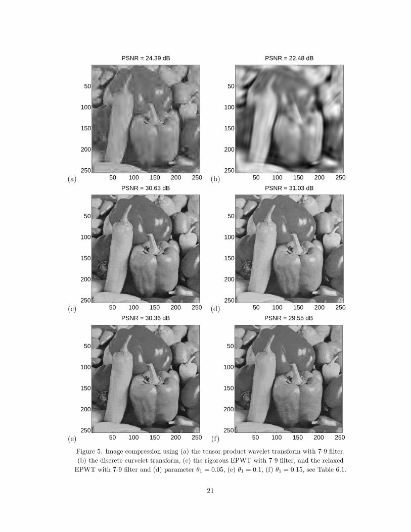
In the first example we consider the 256 × 256 pepper image, i.e. 65536 coefficients(normalized to the range [0, 1)). We are interested in a lossy compression of this image by1024 coefficients, i.e. by 1/64 of the original data. Here, we consider the relaxed EPWTwith different bounds θ1 ∈ {0, 0.05, 0.1, 0.15} and use the three wavelet transforms givenin a), b), c). We compare these results to the tensor product wavelet transform and to
19

curvelets. The results are summarized in Table 6.1. In Figure 5, we show our compressionresults for the (relaxed) EPWT with the 7-9 biorthogonal wavelet transform and compareit with the tensor product wavelet transform and the curvelet transform.
decomp. number of coeff. PSNR of figurewavelet transform θ1 levels after threshold reconstr. imagetensor prod. Haar 8 1024 23.90tensor prod. Daub. 7 1024 24.81tensor prod. 7-9 5 1024 24.39 4(a)
tensor prod. Haar 8 4096 29.88tensor prod. Daub 7 4096 31.16tensor prod. 7-9 5 4096 30.57
EPWT Haar 0.00 16 1024 30.44EPWT Haar 0.05 16 1024 30.55EPWT Haar 0.10 16 1024 29.65EPWT Haar 0.15 16 1024 28.59
EPWT Daubechies 0.00 14 1024 31.20EPWT Daubechies 0.05 14 1024 31.43EPWT Daubechies 0.10 14 1024 30.71EPWT Daubechies 0.15 14 1024 29.73EPWT 7-9 filter 0.00 12 1024 30.63 4(c)EPWT 7-9 filter 0.05 12 1024 31.03 4(d)EPWT 7-9 filter 0.10 12 1024 30.36 4(e)EPWT 7-9 filter 0.15 12 1024 29.55 4(f)
Table 6.1. Comparison of tensor product wavelet transform and easy path wavelet transformfor the pepper image.
Applying the redundant discrete curvelet transform (see in the Matlab toolboxwww.curvelet.org the function fdct wrapping demo recon.m) one obtains 184985 curveletcoefficients for the pepper image. Using 1% threshold, i.e. 1850 coefficients, the recon-structed image achieves an PSNR of 22.48, see Figure 5(b).
Let us now consider the cost of adaptivity for the rigorous and the relaxed EPWT.With the method described in Section 4, we determine the path p16 of length 216 = 65536for the pepper image. In particular, if the path is interrupted after p16(l) (resp. p16(l))we use the following procedure for finding a starting index p16(l + 1) for a new pathway.
We take the vector n of all admissible indices, i.e., all indices in {0, 1, . . . , 65535} thathave not been used in (p16(ν))lν=0 (ordered by size). Let K be the lenght of this vectorand compute k0 := �K/7�. If k0 = 0, i.e., K < 7 then let n0 := n. If k0 > 0 we considerthe vector n0 := (n(1),n(1 + k0),n(1 + 2k0), . . . ,n(1 + 6k0)) of length 7. As a startingindex p16(l + 1) for a new pathway we now choose n(1 + ν0k0), where
ν0 := argminν
|f16(p16(l)) − f16(n(1 + νk0))|, ν = 0, . . . , 6,
and we take p16(l + 1) := ν0.
20
(a)
PSNR = 24.39 dB
50 100 150 200 250
50
100
150
200
250(b)
PSNR = 22.48 dB
50 100 150 200 250
50
100
150
200
250
(c)
PSNR = 30.63 dB
50 100 150 200 250
50
100
150
200
250(d)
PSNR = 31.03 dB
50 100 150 200 250
50
100
150
200
250
(e)
PSNR = 30.36 dB
50 100 150 200 250
50
100
150
200
250(f)
PSNR = 29.55 dB
50 100 150 200 250
50
100
150
200
250
Figure 5. Image compression using (a) the tensor product wavelet transform with 7-9 filter,(b) the discrete curvelet transform, (c) the rigorous EPWT with 7-9 filter, and the relaxed
EPWT with 7-9 filter and (d) parameter θ1 = 0.05, (e) θ1 = 0.1, (f) θ1 = 0.15, see Table 6.1.
21

Observe, that with this procedure one may obtain a starting point of a new pathwaywhose eight neighbors are all admissible such that also the number 7 can occur in p16.Table 6.2 shows the distribution of the numbers 0, . . . , 7 in the path p16 and its entropyfor different bounds θ1. Observe that the path vectors p16 resp. p16 do not depend on theused wavelet transform.
θ1 0.0 0.05 0.1 0.15occurrence of 0 27636 58445 62556 63753occurrence of 1 13494 3117 1207 705occurrence of 2 9250 1610 694 359occurrence of 3 6889 1031 438 275occurrence of 4 4107 590 260 172occurrence of 5 2456 361 185 117occurrence of 6 1685 382 195 155occurrence of 7 19 0 1 0
entropy (bit per pixel) 2.30 0.73 0.37 0.24
Table 6.2. Distribution of numbers 0, . . . , 7 in the path p16 and its entropy for different boundsθ1 for the pepper image.
The path vectors for the further levels (p15, . . . ,p1) have together the length 216 − 1and storing of them usually doubles the cost given in Table 6.2. Using different wavelettransforms, we have found no essential differences in adaptivity costs.
For a rough comparison of the complete storing costs of the compressed pepper im-age using the tensor product transform and the relaxed EPWT we apply the followingsimplified scheme. We compute the cost for coding of the position of M non-zero waveletcoefficients by −M
N log2MN − (N−M)
N log2(N−M)
N , where N = 256× 256 is the number of allcoefficients in the image. Further, let b be the number of bits for encoding of one waveletcoefficient. For the tensor product wavelet transform, the storing costs are composed ofthe costs for encoding of the position of the non-zero coefficients and the costs for storageof these coefficients. For the EPWT, we have in addition the storage cost of the path. Forb = 8 and b = 16, we have compared these costs for the Haar wavelet transform in Table6.3, where we have used the above computed entropy of the path p16 as additional pathcost. Obviously, the EPWT performs especially well for large b.
wavelet transform θ1 number of coeff. b storage costafter threshold (in bpp)
tensor prod. Haar - 4096 8 0.62EPWT Haar 0.10 1024 8 0.61EPWT Haar 0.15 1024 8 0.48
tensor prod. Haar - 4096 16 1.12EPWT Haar 0.10 1024 16 0.74EPWT Haar 0.15 1024 16 0.61
Table 6.3. Comparison of complete storage costs for the pepper image.
22

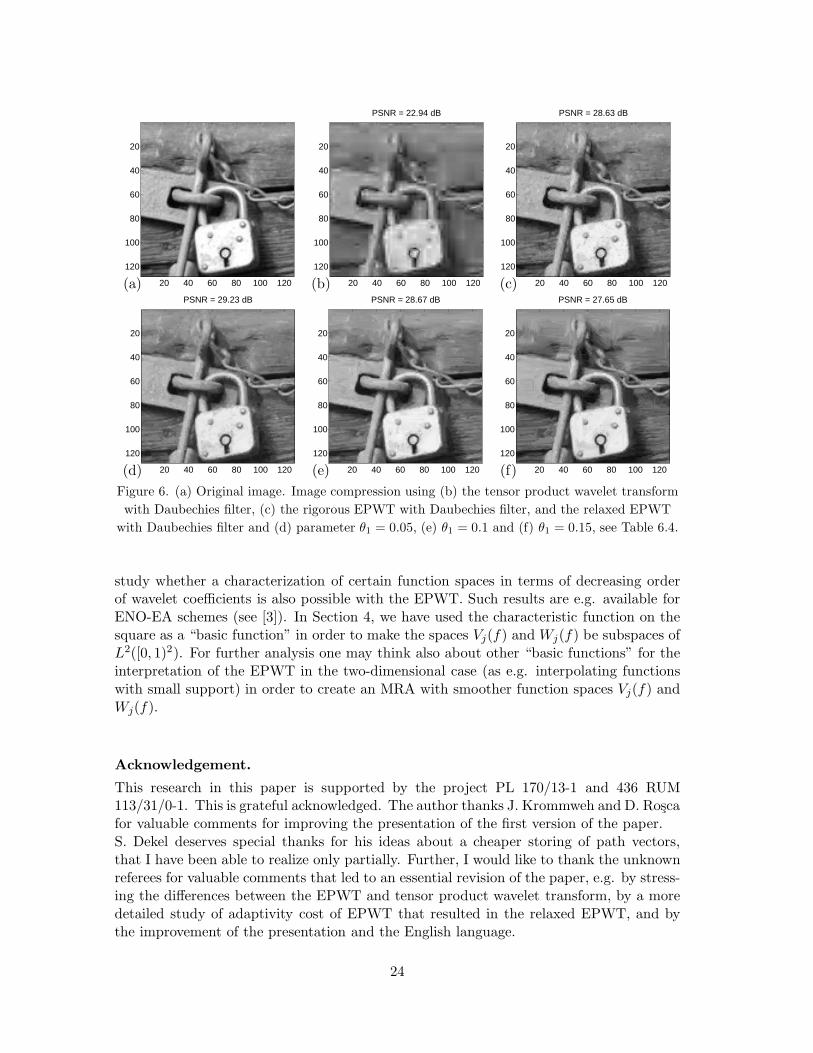
In the second example we are particularly interested in the ability of the EPWT tocompress directional structures of a function. For that purpose we use the 128×128 imageof a door lock with 214 = 16384 coefficients (normalized to the range [0, 1)), see Figure 6(a).As before, we compare the reconstructed images after a wavelet shrinkage procedure with512 remaining coefficients (compression ratio 1/64) for tensor product periodic wavelettransform and the relaxed EPWT with different bounds θ1. The results for the tensorproduct wavelet transform and for the EPWT are summarized in Table 6.4.
θ1 decomp. number of coeff. PSNR of entropy fig.wavelet transform levels after threshold recon. image of p14
tensor prod. Haar - 7 512 22.16 -tensor prod Daub. - 6 512 22.94 - 5(b)tensor prod 7-9 - 4 512 22.49 -EPWT Haar 0.00 14 512 28.04 2.22EPWT Haar 0.05 14 512 28.37 1.11EPWT Haar 0.10 14 512 27.74 0.55EPWT Haar 0.15 14 512 26.85 0.32EPWT Daub. 0.00 12 512 28.63 2.22 5(c)EPWT Daub. 0.05 12 512 29.23 1.11 5(d)EPWT Daub. 0.10 12 512 28.67 0.55 5(e)EPWT Daub. 0.15 12 512 27.65 0.32 5(f)EPWT 7-9 0.00 10 512 28.35 2.22EPWT 7-9 0.05 10 512 28.99 1.11EPWT 7-9 0.10 10 512 28.38 0.55EPWT 7-9 0.15 10 512 27.69 0.32
Table 6.4. Comparison of tensor product wavelet transform and easy path wavelet transform forthe door lock image.
7 Conclusion
As we can see from the examples (see Table 6.1), compared with the traditional tensorproduct wavelet transform, the new EPWT needs less than one fourth of wavelet coeffi-cients in order to achieve a similar PSNR. Here one needs to keep in mind, that with thetwo transforms not only the real wavelet coefficients themselves but also there positionsin the wavelet vectors have to be stored.
For the EPWT we also have to store the path vectors, thus it is highly desirable tomake these vectors as cheap as possible. The idea of relaxed EPWT is a first step in thisdirection. In our numerical experiments we have observed that the performance of therelaxed EPWT crucially depends on the choice of path vectors in all levels. Thereforeone should think about other versions of relaxed EPWT with high performance and muchcheaper path vectors. Instead of the simple method of favorite directions one may usemore sophisticated extrapolation methods for obtaining the next component of the path.
The EPWT may be also interesting for further theoretical investigations regardingthe nonlinear approximation of two-dimensional functions. In the future, we want to
23
(a) 20 40 60 80 100 120
20
40
60
80
100
120
(b)
PSNR = 22.94 dB
20 40 60 80 100 120
20
40
60
80
100
120
(c)
PSNR = 28.63 dB
20 40 60 80 100 120
20
40
60
80
100
120
(d)
PSNR = 29.23 dB
20 40 60 80 100 120
20
40
60
80
100
120
(e)
PSNR = 28.67 dB
20 40 60 80 100 120
20
40
60
80
100
120
(f)
PSNR = 27.65 dB
20 40 60 80 100 120
20
40
60
80
100
120
Figure 6. (a) Original image. Image compression using (b) the tensor product wavelet transformwith Daubechies filter, (c) the rigorous EPWT with Daubechies filter, and the relaxed EPWT
with Daubechies filter and (d) parameter θ1 = 0.05, (e) θ1 = 0.1 and (f) θ1 = 0.15, see Table 6.4.
study whether a characterization of certain function spaces in terms of decreasing orderof wavelet coefficients is also possible with the EPWT. Such results are e.g. available forENO-EA schemes (see [3]). In Section 4, we have used the characteristic function on thesquare as a “basic function” in order to make the spaces Vj(f) and Wj(f) be subspaces ofL2([0, 1)2). For further analysis one may think also about other “basic functions” for theinterpretation of the EPWT in the two-dimensional case (as e.g. interpolating functionswith small support) in order to create an MRA with smoother function spaces Vj(f) andWj(f).
Acknowledgement.
This research in this paper is supported by the project PL 170/13-1 and 436 RUM113/31/0-1. This is grateful acknowledged. The author thanks J. Krommweh and D. Roscafor valuable comments for improving the presentation of the first version of the paper.S. Dekel deserves special thanks for his ideas about a cheaper storing of path vectors,that I have been able to realize only partially. Further, I would like to thank the unknownreferees for valuable comments that led to an essential revision of the paper, e.g. by stress-ing the differences between the EPWT and tensor product wavelet transform, by a moredetailed study of adaptivity cost of EPWT that resulted in the relaxed EPWT, and bythe improvement of the presentation and the English language.
24

References
[1] S. AMAT, F. ARANDIGA, A. COHEN, R. DONAT, G. GARCIA and M. VONOEHSEN, Data compression with ENO schemes - a case study, Appl. Comput. Har-mon. Anal. 11 (2002), 273–288.
[2] F. ARANDIGA, A. COHEN, R. DONAT, N. DYN, Interpolation and approximationof piecewise smooth functions, SIAM J. Numer. Anal. 43 (2005), 41–57.
[3] F. ARANDIGA, A. COHEN, R. DONAT, N. DYN, B. MATEI, Approximation ofpiecewise smooth functions and images by edge-adapted (ENO-EA) nonlinear mul-tiresolution techniques, Appl. Comput. Harmon. Anal., to appear.
[4] E.J. CANDES, D.L. DONOHO, New tight frames of curvelets and optimal represen-tations of objects with piecewise singularities, Comm. Pure Appl. Math. 57 (2004),219–266.
[5] E.J. CANDES, L. DEMANET, D.L. DONOHO, L. YING, Fast discrete curvelettransforms, Multiscale Model. Simul. 5 (2006), 861–899.
[6] R.L. CLAYPOOLE, G.M. DAVIS, W. SWELDENS, R.G. BARANIUK, Nonlinearwavelet transforms for image coding via lifting, IEEE Trans. Image Process. 12 (2003)1449–1459.
[7] A. COHEN, B. MATEI, Compact representation of images by edge adapted multiscaletransforms. in Proc. IEEE Int. Conf. on Image Proc. (ICIP), 2001, Thessaloniki,Greece, pp. 8-11.
[8] I. DAUBECHIES, Ten Lectures on Wavelets, SIAM, Philadelphia, 1992.[9] S. DEKEL and D. LEVIATAN, Adaptive multivariate approximation using binary
space partitions and geometric wavelets, SIAM J. Numer. Anal. 43 (2006), 707–732.[10] L. DEMANET and L. YING, Wave atoms and sparsity of oscillatory patterns, Appl.
Comput. Harmon. Anal. 23 (2007) 368–387.[11] L. DEMARET, N. DYN, and A. ISKE, Image compression by linear splines over
adaptive triangulations. Signal Processing 86 (2006), 1604–1616.[12] R.A. DEVORE, Nonlinear approximation, Acta Numerica, A. Iserles (Ed.), Cam-
bridge University Press, Cambridge, 1998, p. 51–150.[13] M.N. DO and M. VETTERLI, The contourlet transform: An efficient directional
multiresolution image representation, IEEE Trans. Image Process. 14 (2005) 2091–2106.
[14] D.L. DONOHO, Wedgelets: Nearly minimax estimation of edges, Ann. Stat. 27(1999), 859–897.
[15] K. GUO and D. LABATE, Optimally sparse multidimensional representation usingshearlets, SIAM J. Math. Anal. 39 (2007), 298–318.
[16] K. GUO, W.-Q. LIM, D. LABATE, G. WEISS, and E. WILSON, Wavelets withcomposite dilations, Electr. res. Announc. of AMS 10 (2004), 78–87.
[17] A. HARTEN, Discrete multiresolution analysis and generalized wavelets, J. AppliedNum. Math. 12 (1993), 153–193.
[18] A. HARTEN, Multiresolution representation of data: general framework, SIAM J.Numer. Anal. 33 (1996), 1205–1256.
25

[19] L. JACQUES, J.-P. ANTOINE, Multiselective pyramidal decomposition of images:wavelets with adaptive angular selectivity, Int. J. Wavelets Multiresolut. Inf. Process.5 (2007), 785–814.
[20] E. Le PENNEC, and S. MALLAT, Bandelet image approximation and compression,Multiscale Model. Simul. 4 (2005), 992–1039.
[21] S. MALLAT, A wavelet tour of signal processing, Academic Press, San Diego, 1999.
[22] S. MALLAT, Geometrical grouplets, Appl. Comput. Harmon. Anal. (2009), to appear.[23] B. MATEI, Methods multiresolution no-lineaires - Applications au traitement
d’image, PhD dissertation, Universite Paris VI, 2002.
[24] B. MATEI, Smoothness characterization and stability in nonlinear multiscale frame-work: theoretical results, Asymptotic Anal. 41 (2005), 277–309.
[25] D.D. PO and M.N. DO, Directional multiscale modeling of images using the contourlettransform, IEEE Trans. Image Process. 15 (2006), 1610–1620.
[26] R. SHUKLA, P.L. DRAGOTTI, M.N. DO, and M. VETTERLI, Rate-distortion op-timized tree structured compression algorithms for piecewise smooth images, IEEETrans. Image Process. 14 (2005), 343–359.
[27] M.B. WAKIN, J.K. ROMBERG, H. CHOI, and R.G. BARANIUK, Wavelet-domainapproximation and compression of piecewise smooth images, IEEE Trans. Image Pro-cess. 15 (2006), 1071–108.
26