The effect of consumer switching costs on market powerof cable television providers

Oleksandr Shcherbakov

November 2009

[Preliminary and incomplete]

Abstract

This paper empirically evaluates the effect of consumer switching costs on marketpower of cable television providers. To do so I propose an algorithm to estimate supplyside parameters when the demand side is represented by consumers with persistent het-erogeneity in tastes and state-dependent utility. Under such conditions, regardless ofwhether consumers are forward-looking or behave in a myopic way, the demand sched-ule introduces dynamics into the producer problem. Presence of multiple state variablesmakes full solution to the producer dynamic programming problem difficult or compu-tationally infeasible. Therefore, I estimate supply side parameters from the optimalityconditions for the dynamic controls. Using data from the paid television markets in US,I estimate cost functions of the cable television providers. In these markets, persistentconsumer heterogeneity and state dependence due to switching costs requires producersto keep track of the entire distribution of consumer types which enters states space ofa dynamic programming problem. Preliminary estimates of the consumer switchingcosts are $149 and $238 for cable and satellite providers respectively. The estimatesof the supply side parameters imply average cost of providing service per subscriber of$2.19 and average per subscriber price-cost margin of $16.52. Counterfactual simula-tions suggest that without switching costs cable prices would be 28 percent higher withsatellite competitors and 51 percent higher in case of static monopoly scenario.

1 Introduction

This paper pursues two objectives. The first one is to assess the economic effects of consumerswitching costs in the paid-television industry on market structure and social welfare. Toaccomplish this task I need to evaluate the impact of switching costs on the optimal choices

1

of prices and quality levels by cable television providers. This, in turn, requires knowledgeof the costs structure of the cable firms.

Estimation of the supply side parameters becomes a challenging task if consumer utilityexhibits state-dependence generated by the non-trivial switching costs. State-dependentdemand, in turn, requires considering price and quality choices by the producers in a dynamicperspective. This is true regardless of whether consumers make myopic or forward-lookingdecisions. With multiple consumer types and/or many products in the market the statespace of the producer dynamic programming problem becomes very large. Large state spacerenders traditional solutions to the producer problem computationally infeasible. Hence, thesecond objective of this paper is to develop a methodology that makes estimation of thesupply side parameters possible.

In order to overcome the large state space problem I suggest estimation from the first-order conditions for dynamic controls similar (but not identical) to Berry and Pakes (2001).A modified generalized instrumental variables technique for non-linear rational expectationsmodels originally proposed by Hansen and Singleton (1982) could be used to estimate pa-rameters of the cable company cost function. Presence of multiple state variables that aresimultaneously shifted by a single dynamic control makes it impossible to express the first-order conditions in terms of primitives of the model, i.e. derivatives of the per-period rewardand transition functions. To obtain partial derivatives of the value function with respect toeach state I use forward simulation approach developed in Hotz et al. (1994) for single-agentdecision problems and extended in Bajari et al. (2007) to a dynamic games environment.

Simulation approach consists of three steps. In the first step, I estimate demand sidemodel and recover the distribution of the consumer types across market shares and un-observed cable and satellite service characteristics. In the second step, I estimate policyfunctions defined on the producer state space and the law of motion for the exogenous statevariables. In the third step, parameters of the cost function are estimated from the first-order conditions for the producer dynamic programming problem. The main difference fromBajari et al. (2007) is in the first step, which is necessary to recover unobserved producerstate variables.

Similar to Bajari et al. (2007), there are considerable computation benefits if per-periodproducer reward function is linear in parameters. In this case, computationally intensesimulation of the derivatives of the value function needs to be conducted only once for a setof basis functions. When estimating supply-side parameters the vector of basis functions issimply scaled by the current values of the parameter vector. This makes estimation procedurevery fast and comparable in terms of computation time to a standard GMM procedure fornon-linear models.

To estimate parameters of the demand and supply models I use data on 564 U.S. cablesystems in 1992-2002. Preliminary estimates of the demand side parameters suggest switchingcosts of $149 and $238 for cable and satellite providers respectively. At this stage, thedemand side estimates cannot reject a representative consumer model, although mean levels

2

of switching costs as well as price and quality coefficients are estimated precisely. Supply-side estimates imply the average cost of providing service per subscriber of about $2.19and average price-cost margin of $16.52. Under counterfactual scenario where there are noswitching costs and satellite policy as well as the values of own cable companies’ cost shiftersremain unchanged cable prices are estimated to be 28 percent higher than the observed level.In a static monopoly scenario, where there are no satellite competitor and no switching costscable prices are on average 51 percent higher than the observed ones.

The remainder of the paper is organized as follows. Section 2 discusses related literature.Sections 3 and 4 provide institutional details for the paid-television industry in U.S. anddescribe data used for estimation. In sections 5 and 6 I describe demand and supply modelsand corresponding estimation strategies and outline differences in estimation algorithm formyopic and dynamic consumers. Section 7 discusses instrumental variables and identificationissues and section 8 presents preliminary estimation results. Section 9 outlines strategy forsimulating counterfactual scenarios of the industry evolution and section 10 concludes.

2 Related literature

Despite a large theoretical literature on switching costs, there are only a few empirical studies.Several examples of industries with consumer switching costs include banking (Sharpe (1997),Kiser (2002), Kim et al. (2003)), auto insurance (Israel (2003)), airline (in relation to frequentflyer programs; Borenstein (1992)), long-distance telephone service (Knittel (1997)), andretail electricity industries (Salies (2005), Sturluson (2002)).

The limited number of empirical studies on the topic may reflect the difficulty of measuringswitching costs, which are not directly observable in the data. One of the widely cited papersin the field is Shy (2002). He suggests a framework for quick and easy estimation of switchingcosts. Under a set of assumptions, the author shows how switching costs can be directlyinferred from observed prices and market shares. Unfortunately, the underlying assumptionsare very strong, and include homogeneous products and static behavior on both the demandand supply side. Two other papers that attempt to empirically measure switching costsin the framework of dynamically optimizing consumers are Schiraldi (2006) and Ho (2009).Both papers use modified versions of the nested fixed point estimation algorithm developedin Gowrisankaran and Rysman (2007) for estimation of dynamic demand for durable goods.

While I specify and estimate a model of consumer behavior in markets with switching coststhis is not the primary objective of the present paper. The major focus is on a methodologythat allows estimating supply side parameters, namely parameters of the cost function, inpresence of state dependent consumer utility. State dependence on the demand side calls fora forward looking behavior on the supply side. In presence of many state variables traditionalsolution to the producer dynamic programming problem becomes computationally infeasible.Hence, alternative estimation approaches are needed.

3

There are only a few empirical papers that attempt to address the question. The first oneis Dube et al. (2008) where the authors estimate the demand side with many heterogeneousconsumers. To solve for the dynamically optimal pricing policy they assume a stationarylong-run equilibrium, which allows using Euler equation framework. It is worth noting thatthis is rather a computational theory paper (in its supply side part) that calculates alternativeoptimal pricing policies under a set of very restrictive assumptions, including steady state andno uncertainty on the producer side. Another paper in the area is Che et al. (2006) who dealwith the problem of large state space by imposing bounded rationality assumption on thefirms behavior, when the distribution of the consumer types across products is summarizedby its first moments.

It is worth noting that one of the possible solutions to the problem of many state vari-ables in macro literature was suggested in Krusell and Smith (1998). The idea is that thedistribution of consumer types could be approximated reasonably well with only a finite setof its first moments. However, in case of several products state-dependence requires keepingtrack of these moments for each product. Hence, with the increase in the number of productssolution to the producer dynamic programming problem quickly becomes infeasible.

3 Institutional details

Cable television, formerly known as Community Antenna Television or CATV, emerged inthe late 1940s in Arkansas, Oregon and Pennsylvania to deliver broadcast signals to theremote areas with poor over-the-air reception.1 In these areas homes were connected to theantenna towers located at the high points via cable network. Starting with 70 cable systemsserving about 14,000 subscribers in 1952, a decade later almost 800 cable systems servedabout 850,000 subscribers (ibid.). According to FCC (2000), by October 1998 the number ofcable systems reached 10,700 providing service to more than 65 million subscribers in 32,000communities.

The ability of cable systems to “import” distant signals imposed a significant competitivepressure on the local television stations, which eventually has led to a regulatory restrictionsby the FCC on the programming content of cable companies first introduced in 1965-66.Gradual deregulation of cable industry began in the early 1970s, which when accompaniedwith the development of satellite communication technology has led to an emergence of na-tional networks (e.g. HBO in 1972, Showtime in 1976, ESPN in 1979), which programmingwas distributed by satellite to cable systems nationwide. Considerable investment activityin the industry resumed after the 1984 Cable Communications Policy Act that establisheda more favorable regulatory environment. In 1992, continuing increase in the cable pricesresulted in another waive of regulatory intervention, when Congress enacted the Cable Televi-

1See National Cable & Telecommunications Association (NCTA), http://www.ncta.com/About/About/HistoryofCableTelevision.aspx (accessed March 01, 2009).

4

sion Consumer Protection and Competition Act of 1992. Despite new regulatory restrictionsthe industry continued its growth. At about the same time, a new competing technology -direct broadcast satellite - challenged previously “exclusive” cable programming.

The 1996 Telecommunications Act introduced a dramatic change in the public policy fortelecommunication services towards further deregulation of the industry. A major upgradeof the cable distribution networks amounting to about $65 billion of investment between1996 and 2002 resulted in an increased amount of hybrid networks of fiber optic and coaxialcable (see an overview of cable history by NCTA). These high capacity networks allowed fora multi-channel video, two-way voice, high-speed internet access and high definition digitalvideo services. In the late 90s, most cable systems had capacity ranging between 36 and 60channels and some offered more than 100 channels. Most cable subscribers receive servicefrom a system offering more than 54 channels (FCC (2000)). In some cases, cable companiescreated own programming as well as provided leased access channels to those wishing to showspecific programs. Other home services that are possible using the two-way transmission cablenetworks include video on demand, interactive TV, electronic banking, shopping, utility meterreading, etc.

Until the 1990s, local cable systems were effectively natural monopolies as they facedvirtually no competition except in a few cases of ”overbuilt” systems where the same locationwas served by more than one cable company. Competition from the C-Band satellite (apredecessor to today’s DBS systems) was very limited because of extremely high setup costs.DBS service was launched in the early 90s and originally was popular mostly in rural areaswhere cable service did not exist. Since then the number of subscribers of DBS providers hasexperienced rapid growth.

Table 1: DBS penetration rates in 2001-20042001 2004 Change

Rural 26% 29% 12%Suburban 14% 18% 29%Urban 9% 13% 44%

Source: GAO report to the U.S. Senate, April 2005

Due to technological restrictions, DBS cannot match most of the supplementary servicesoffered by the cable companies. Until recently, some differences in the programming contentwere induced by industry regulation. Prior to 1999, when the Congress enacted the SatelliteHome Viewer Improvement Act, DBS carriers were not allowed to broadcast local channels.In many cases this was considered a competitive disadvantage of satellite providers (see FCC4th annual report on competition in markets for video programming, as of January 13, 1998).

DBS and cable operators use different quality and price setting strategies. While eachcable system makes pricing and quality decisions locally, satellite operators set these variables

5

at the national level. It is conceivable though that there are other factors, like customerservice as well as landscape and weather conditions that effect the quality of reception andattractiveness of the satellite service at regional level.

Switching costs in the television industry are primarily transactional. They include notonly upfront equipment and installation fees but also hassle costs. Even though many cablecompanies do not require purchasing equipment (it is rather rented by the cable subscribers),anecdotal evidence suggests that the cost of returning rented equipment may be substantial.In what follows I use terms “start-up costs” and “switching costs” interchangeably. An-other component of the switching costs are “shopping costs” associated with the purchase ofsupplementary services like telephone and internet.

4 Data

In order to measure the economic effects of switching costs I use data from the US paidtelevision industry in 1992-2002. Most variables for the cable providers come from the War-ren’s Factbook editions. Satellite data was collected from the internet sources and covers1997-2002.

For the empirical estimation part of the paper I define market to be an area franchisedto the cable company. In all of the markets used for estimation there is only a single cablesystem, i.e. none of the “overbilders” are included.

Even though cable and satellite providers often offer more then one programming tier, Imaintain a single service assumption.2 Thus, for cable it is either Basic or Expanded Basicdepending on the number of subscribers and for satellite it is Total Choice (DIRECTV) tier.

For estimation I used a sample of 564 cable systems that have reliable data on marketshares, price and quality variables for 1992-2002. Below I describe several issues with thedata.

Satellite penetration rates are available only at the Designated Market Area (DMA) level.In order to compute satellite market share for each of the more narrowly defined marketsI used an assumption similar to one in Chu (2007). Within a DMA satellite subscribersconstitute a constant proportion of the non-cable subscribers. Define

Rkt =#satsubskt

Mkt −#cabsubskt

where k and t are DMA and time subscripts; #satsubskt is the number of satellite subscribers;Mkt is the total number of households; and #cabsubskt is the number of cable subscribers.Then satellite market share in market j located in DMA k is computed as

ssjt = (1− scjt)Rkt

2There are no conceptual difficulties in including multiple tiers. It is rather data limitations, when thenumber of missing observations for more advanced tiers is too large.

6

The rationale for this assumption is related to the timing of the entry by DBS. In thefirst place, satellite providers target areas where there is no alternative cable paid-televisionservice or where the cable share is small. Therefore, one can expect that within the sameDMA satellite penetration is relatively larger in the areas franchised to the cable systemswith smaller market shares. Typically, satellite penetration is greater in rural and subur-ban than in the densely populated urban areas where cable companies have greater marketshares.3 Geographic variation in satellite penetration rates is supported by official statistics(see Section 3).

Besides, DMA level satellite penetration rates are available only from 1997. In orderto deal with the initial conditions problem (as discussed in section 6.1), I imputed satelliteshares at the local markets level by using the national level dynamics. For this reason, toform the empirical moment conditions I use data in 1997-2002 only.4

Another important question is the definition of the quality of programming content offeredby a particular provider. Using number of channels offered as a proxy for quality of thesystem’s programming may be problematic. In particular, such a proxy would not capturechanges in the programming composition, holding the number of channels constant. In manycases, the data reveal that a lot of variation in the quality variable is due to the change in thecomposition of channels rather than due to change in the number of channels. In order tocontrol for different compositions of channels I used data on the average cost of each channelcharged by the television networks. Channels with unknown or zero costs were assigned acost of $0.01.

Price data for cable and satellite services was adjusted using consumer price index with1997 as the base year. Hence, any monetary equivalents computed in this paper are in 1997prices. Summary statistics for the key variables is listed in the table 2

5 Model

In this section I discuss demand and supply side models of the paid television industry. Onthe demand side, consumers are persistently heterogeneous with respect to their switchingcosts and tastes for service characteristics. Presence of switching costs results in state-dependence when each consumer’s last period choice affects current utility. State-dependence,in turn, calls for the forward-looking consumer behavior. However, it is not clear if the gains

3Another reason to expect lower satellite penetration in urban areas is the necessity to locate receiver(dish) in a place that guarantees open access to the orbital satellite. In urban areas it was harder due to thepresence of multistory buildings that may impede receiving satellite beams. Besides in multi-unit structuresup until recently to install a dish a resident must obtain permission of the home owner, which was not alwaysan easy task.

4Data from 1992-1996 are used only to approximate the initial distribution of consumer types acrossmarket shares.

7

Table 2: Descriptive statistics for the key variables, 564 systems, 6054 observationsVariable min max mean med s.d.

Market share (cable) 0.011 0.867 0.426 0.438 9.157Market share (satellite) 0.001 0.364 0.083 0.074 0.065Price (cable) 3.551 34.20 19.20 20.52 5.869Price (satellite) 24.80 34.74 29.85 29.99 3.687Quality (cable) 0.02 9.570 3.338 3.06 1.558Quality (satellite) 4.49 10.42 5.826 4.49 2.087Capacity (cable) 10 134 39.78 36 13.58Miles coaxial lines (cable),’000 0.001 4.491 0.111 0.020 0.301

Source: own calculations

from a dynamically optimal behavior justifies costs of finding such an optimal strategy.5

In the present paper, I focus primarily on the supply side and maintain an assumption ofconsumer myopia for the reasons of computational simplicity. However, whenever relevantI provide quick asides on the modifications necessary to incorporate dynamic considerationsinto the demand-side model. Dynamic demand estimates using the same data can be foundin Shcherbakov (2008). Moreover, as I discuss below, the suggested supply-side estimationstrategy need not change under alternative assumptions on the consumer rationality as longas the estimation of the demand relationship does not depend on the parameters of the supplyside.

5.1 Demand side: myopic consumers

Let J = o, c, s denote consumer choice set consisting of cable, c, satellite, s, and an outsideoption of no paid TV, o. There is a number of persistently heterogeneous consumer typeswhose (time-invariant) preferences are given by iid draws from a distribution known up to aparameter vector. Within each type there is a continuum of non-persistently heterogeneousconsumers. With some abuse of notation both types of heterogeneity will be subscribed withi.

Cable and satellite television is characterized by two observable characteristics: monthlysubscription fee, pjt, and quality index, qjt. In addition, there is a scalar, ξjt, representingservice characteristics observed by the market participants, but unobserved by an econome-tricians.

Let ait ∈ J denote consumer choice in period t. First time subscription to service jis associated with time-invariant monetary and hassle costs expressed in utility units, ηij.

5Quantifying such gains goes beyond the scope of the present paper and remains a question for furtherresearch.

8

Assume that disconnection is costless, i.e. ηio = 0 ∀i. Persistent consumer heterogeneity intastes for service has several dimensions. In addition to the type-specific switching costs,each consumer type has idiosyncratic taste for service and different price sensitivity.

Assume that consumer per-period utility function is linear and given by

uijt =

−ηij+ αij + αpi pjt + αqqjt + ξjt + εijt, if ait 6= ait−1,

αij + αpi pjt + αqqjt + ξjt + εijt, otherwise

=

−ηij+ αij + αipjt + δjt + εijt, if ait 6= ait−1,

αij + αipjt + δjt + εijt, otherwise

=

−ηij+ δijt + εijt, if ait 6= ait−1,

δijt + εijt, otherwise

(1)

where δjt = αppjt + αqqjt + ξjt, δijt = αij + αpi pjt + δjt, αp is the population mean price

sensitivity, αpi are each type deviations from the mean, and εit = (εiot, εict, εist)iid∼ Fε(·)

represent (non-persistent) heterogeneity within each discrete consumer type. I normalizeutility from the outside option (over-the-air television) to zero, i.e. uiot = εiot.

Assume that consumers are myopic, i.e. their choices are based on the current periodutility and do not account for the future evolution of service characteristics. Define thefollowing probabilities for consumer type i

Pri(c→ c) = Pr(δict + εict ≥ −ηis + δist + εist, δict + εict ≥ εiot)

Pri(s→ c) = Pr(−ηic + δict + εict ≥ δist + εist,−ηic + δict + εict ≥ εiot)

Pri(o→ c) = Pr(−ηic + δict + εict ≥ −ηis + δist + εist,−ηic + δict + εict ≥ εiot)

Pri(c→ s) = Pr(−ηis + δist + εist ≥ δict + εict,−ηis + δist + εist ≥ εiot)

Pri(s→ s) = Pr(δist + εist ≥ −ηic + δict + εict, δist + εist ≥ εiot)

Pri(o→ s) = Pr(−ηis + δist + εist ≥ −ηic + δict + εict,−ηis + δist + εist ≥ εiot)

Let sijt denote a share of consumer type i choosing product j in period t. Then in anyt > 0 current share of consumer type i subscribed to the cable service is given by

sict =sict−1 · Pri(c→ c) + sist−1 · Pri(s→ c) + (1− sict−1 − sist−1) · Pri(o→ c) (2)

Similarly, current share of consumer type i subscribed to the satellite service is given by

sist =sist−1 · Pri(s→ s) + sict−1 · Pri(c→ s) + (1− sict−1 − sist−1) · Pri(o→ s) (3)

Assumption 1: Consumer heterogeneity parameters εit are represented by iid draws from a

9

distribution known up to a parameter vector, i.e.

εijtiid∼ Extreme V alue Type 1, with density

f(εijt) = exp(−εijt) exp(− exp(−εijt))

By assumption 1 the share of type i choosing cable in the current period is given by

sict =sict−1 ·exp(δict)

1 + exp(δict) + exp(−ηist + δist)

+ sist−1 ·exp(−ηic + δict)

1 + exp(−ηic + δict) + exp(δist)

+ (1− sict−1 − sist−1) ·exp(−ηic + δict)

1 + exp(−ηic + δict) + exp(−ηist + δist)

Individual satellite shares for each type i can be calculated in a similar way.Let me postpone derivation of the aggregate market shares and discuss an alternative

model where consumers are forward-looking.6

5.2 Demand side: forward-looking consumers

In this section, I discuss a possibility to incorporate dynamic considerations into the con-sumer behavior. As long as the formulation of the consumer dynamic programming problemdoes not depend on the parameters of the supply-side, i.e. the demand relationship can beseparately estimated, solution to the multiple state variables problem on the supply side isunaffected.

Consider a forward looking consumer of type i. Time is discrete and indexed by t =0, 1, 2..., horizon is infinite. Suppose per-period utility function of a consumer type i is de-fined as in (1). Let Ωt denote current service characteristics and all other factors that affectfuture service characteristics. The following assumption is typically made in the literatureto reduce the dimensionality of the producer state space.

Assumption 2: Vector Ωt consists of a pair of current utility flows (δict, δist) and it evolvesas a first-order Markov process P (Ωt+1|Ωt) = P (δict+1, δist+1|δict, δist).

It is worth noting that assumption (2) implies bounded rationality in consumer behavior,

6The discussion in the next section follows traditional approach in the empirical IO literature by modelingconsumer expectations with a reduced-form specification of beliefs.

10

when consumers do not explicitly consider producer optimization problem. In practice,this assumption allows for separate estimation of the demand relationship as long as thedata is generated by a market equilibrium and the reduced form specification of the processP (δict+1, δist+1|δict, δist) is flexibly estimated.7

Consumer dynamic programming problem can be written recursively in the form of aBellman equation

Vi(εit, δict, δist, ait−1) =

max

εiot + βE [Vi (εit+1, δict+1, δist+1, ait = o) |εit, δict, δist, ait−1] ,

uict(δict, ait−1) + βE [Vi (εit+1, δict+1, δist+1, ait = c) |εit, δict, δist, ait−1] ,

uist(δist, ait−1) + βE [Vi (εit+1, δict+1, δist+1, ait = s) |εit, δict, δist, ait−1]

(4)

where uijt(δijt, ait−1) are defined as in (1).Under assumption (1) probability that consumer of type i chooses service j in the current

period given last period choice k is

Pr(k → j) = Pr(V kji + εijt ≥ V kl

i + εilt,∀l 6= j)

=expV kj

i∑l expV kl

i

(5)

where

V kji (δict, δist) = V (δict, δist, ait = j, ait−1 = k)

defines “choice-specific” value function net of current idiosyncratic preference draw εijt. Notethat unlike in the case of myopic consumers value of choosing outside alternative today isnot zero as it encapsulates an option to subscribe to one of the paid television providers inthe future. These choice-specific value functions can be computed using joint contractionmapping

V ooi = βE ln[expV oo

i + exp(V cci − ηc) + exp(V ss

i − ηs)],V cci = δict + βE ln[expV oo

i + expV cci + exp(V ss

i − ηs)],V ssi = δist + βE ln[expV oo

i + exp(V cci − ηc) + expV ss

i ](6)

where expectations are taken with respect to future values of (δict, δist) and V kji = −ηij +V jj

i .Then individual market shares for each type of consumers can be calculated similar to

(2) and (3).

7In the modern literature on dynamic demand estimation, assumption (2) is often replaced with a muchstronger assumption on the evolution of the entire market, which is captured by the “logit inclusive values”as in Melnikov (2001), Gowrisankaran and Rysman (2007), Schiraldi (2006).

11

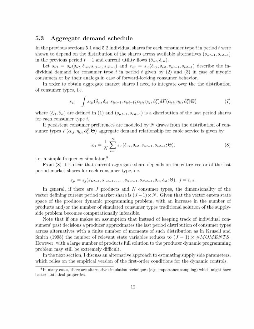
5.3 Aggregate demand schedule

In the previous sections 5.1 and 5.2 individual shares for each consumer type i in period t wereshown to depend on the distribution of the shares across available alternatives (sict−1, sist−1)in the previous period t− 1 and current utility flows (δict, δist).

Let sict = sic(δict, δist, sict−1, sist−1) and sict = sic(δict, δist, sict−1, sist−1) describe the in-dividual demand for consumer type i in period t given by (2) and (3) in case of myopicconsumers or by their analogs in case of forward-looking consumer behavior.

In order to obtain aggregate market shares I need to integrate over the the distributionof consumer types, i.e.

sjt =

∫sijt(δct, δst, sict−1, sist−1;αij, ηij, α

pi )dF (αij, ηij, α

pi |Θ) (7)

where (δct, δst) are defined in (1) and (sict−1, sist−1) is a distribution of the last period sharesfor each consumer type i.

If persistent consumer preferences are modeled by N draws from the distribution of con-sumer types F (αij, ηij, α

pi |Θ) aggregate demand relationship for cable service is given by

sct =1

N

N∑i=1

sic(δict, δist, sict−1, sist−1; Θ), (8)

i.e. a simple frequency simulator.8

From (8) it is clear that current aggregate share depends on the entire vector of the lastperiod market shares for each consumer type, i.e.

sjt = sj(s1ct−1, s1st−1, . . . , sNct−1, sNst−1, δct, δst; Θ), j = c, s.

In general, if there are J products and N consumer types, the dimensionality of thevector defining current period market share is (J−1)×N . Given that the vector enters statespace of the producer dynamic programming problem, with an increase in the number ofproducts and/or the number of simulated consumer types traditional solution of the supply-side problem becomes computationally infeasible.

Note that if one makes an assumption that instead of keeping track of individual con-sumers’ past decisions a producer approximates the last period distribution of consumer typesacross alternatives with a finite number of moments of such distribution as in Krusell andSmith (1998) the number of relevant state variables reduces to (J − 1) × #MOMENTS.However, with a large number of products full solution to the producer dynamic programmingproblem may still be extremely difficult.

In the next section, I discuss an alternative approach to estimating supply side parameters,which relies on the empirical version of the first-order conditions for the dynamic controls.

8In many cases, there are alternative simulation techniques (e.g. importance sampling) which might havebetter statistical properties.

12

5.4 Supply side

On the supply side of the paid television market there are two producers: cable and satelliteproviders of the paid television service. As in the previous sections, variables are indexed bya subscript j ∈ o, c, s.

Time is discrete and is indexed by t = 0, 1, 2, . . . I assume that each provider offers onlya single tier.9 The evolution of price, observed and unobserved quality offered by satelliteprovider is assumed to be exogenous. Therefore, the only strategic player in the market iscable companies.

Prior to making price, pct, and quality, qct, choice cable companies observe price, observedand unobserved (by econometricians) quality of satellite service. In addition, cable providersobserve realizations of own scalar unobservable, ξct, as well realizations of a vector of exoge-nous cost shifters Zct. The above is summarized by the following assumption.

Assumption 3: In each market and each time period a cable company solves a single-agentdecision problem after observing realizations of exogenous variables, xt = (pst, qst, ξst, ξct, Zct).

As discussed in the section (5.3), a cable company faces demand relationship summarizedby the following equation

Dct = Mt ·N∑i=1

sic(pct, qct, xt; sict−1, sist−1) (9)

where Mt is the market size in period t and sic(·) is a function that computes current shareof consumer type i.

Let sit = (sict, sist)′, i = 1, . . . , N denote a pair of cable and satellite shares of consumer

type i in period t. Define st = (sit, . . . , sNt)′ be a 2N × 1 vector of all consumer types shares

in period t.Assume that market size is constant over time, i.e. Mt = M, ∀t then per-period profit of

a cable provider has the following parametric form

Π(st−1, xt, pct, qct) = M ·N∑i=1

sic(sit−1, xt, pct, qct)(pct − c(qct, Zct)), (10)

where c(qct) is a marginal cost of providing quality qct per subscriber. Note that this spec-ification implicitly assumes that the cost function is perfectly scalable in the number ofsubscribers.

9This assumption is mainly driven by the data limitations. Extension to multiple tiers possible anddiscussed later in the paper.

13

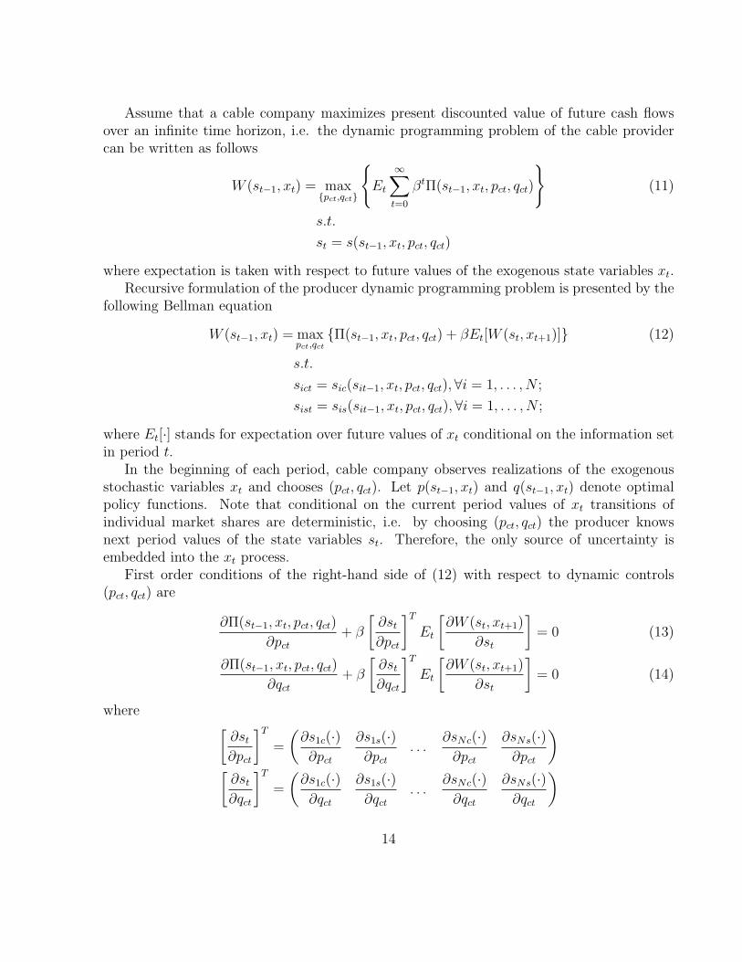
Assume that a cable company maximizes present discounted value of future cash flowsover an infinite time horizon, i.e. the dynamic programming problem of the cable providercan be written as follows

W (st−1, xt) = maxpct,qct

Et

∞∑t=0

βtΠ(st−1, xt, pct, qct)

(11)

s.t.

st = s(st−1, xt, pct, qct)

where expectation is taken with respect to future values of the exogenous state variables xt.Recursive formulation of the producer dynamic programming problem is presented by the

following Bellman equation

W (st−1, xt) = maxpct,qct

Π(st−1, xt, pct, qct) + βEt[W (st, xt+1)] (12)

s.t.

sict = sic(sit−1, xt, pct, qct),∀i = 1, . . . , N ;

sist = sis(sit−1, xt, pct, qct),∀i = 1, . . . , N ;

where Et[·] stands for expectation over future values of xt conditional on the information setin period t.

In the beginning of each period, cable company observes realizations of the exogenousstochastic variables xt and chooses (pct, qct). Let p(st−1, xt) and q(st−1, xt) denote optimalpolicy functions. Note that conditional on the current period values of xt transitions ofindividual market shares are deterministic, i.e. by choosing (pct, qct) the producer knowsnext period values of the state variables st. Therefore, the only source of uncertainty isembedded into the xt process.

First order conditions of the right-hand side of (12) with respect to dynamic controls(pct, qct) are

∂Π(st−1, xt, pct, qct)

∂pct+ β

[∂st∂pct

]TEt

[∂W (st, xt+1)

∂st

]= 0 (13)

∂Π(st−1, xt, pct, qct)

∂qct+ β

[∂st∂qct

]TEt

[∂W (st, xt+1)

∂st

]= 0 (14)

where [∂st∂pct

]T=

(∂s1c(·)∂pct

∂s1s(·)∂pct

. . .∂sNc(·)∂pct

∂sNs(·)∂pct

)[∂st∂qct

]T=

(∂s1c(·)∂qct

∂s1s(·)∂qct

. . .∂sNc(·)∂qct

∂sNs(·)∂qct

)

14

and

[∂W (st, xt+1)

∂st

]=

∂W (st, xt+1)

∂s1ct

∂W (st, xt+1)

∂s1st...

∂W (st, xt+1)

∂sNct

∂W (st, xt+1)

∂sNst

Consider ith elements of the vector

[∂st∂pct

]. The implications of the assumption 1 are as

follows

∂sic(·)∂pct

=sict−1∂Pri(c→ c)

∂pct+ sist−1

∂Pri(s→ c)

∂pct+ (1− sict−1 − sist−1)

∂Pri(o→ c)

∂pct

=αpi

sict−1 ·(Pri(c→ c)− Pr2

i (c→ c))

+ sist−1 ·(Pri(s→ c)− Pr2

i (s→ c))

+ (1− sict−1 − sist−1) ·(Pri(o→ c)− Pr2

i (o→ c))

∂sis(·)∂pct

=sist−1∂Pri(s→ s)

∂pct+ sict−1

∂Pri(c→ s)

∂pct+ (1− sict−1 − sist−1)

∂Pri(o→ s)

∂pct

=− αpi

sist−1 · Pri(s→ s) · Pri(s→ c)

+ sict−1 · Pri(c→ s) · Pri(c→ c)

+ (1− sict−1 − sist−1) · Pri(o→ s) · Pri(o→ c)

15

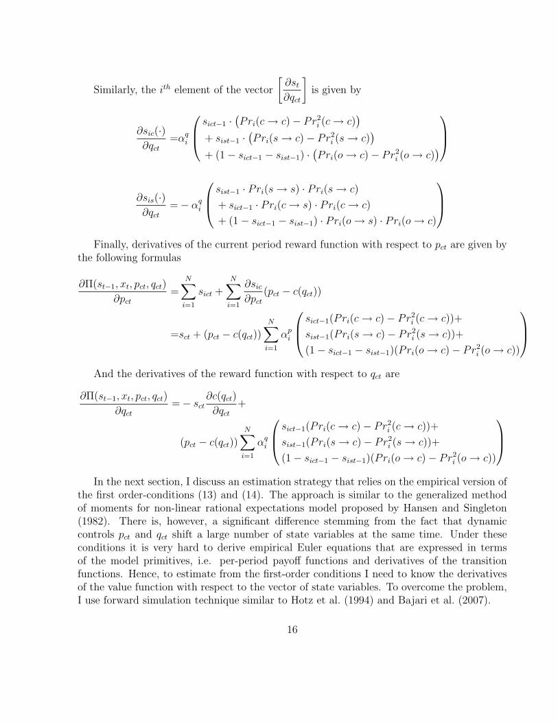
Similarly, the ith element of the vector

[∂st∂qct

]is given by

∂sic(·)∂qct

=αqi

sict−1 ·(Pri(c→ c)− Pr2

i (c→ c))

+ sist−1 ·(Pri(s→ c)− Pr2

i (s→ c))

+ (1− sict−1 − sist−1) ·(Pri(o→ c)− Pr2

i (o→ c))

∂sis(·)∂qct

=− αqi

sist−1 · Pri(s→ s) · Pri(s→ c)

+ sict−1 · Pri(c→ s) · Pri(c→ c)

+ (1− sict−1 − sist−1) · Pri(o→ s) · Pri(o→ c)

Finally, derivatives of the current period reward function with respect to pct are given by

the following formulas

∂Π(st−1, xt, pct, qct)

∂pct=

N∑i=1

sict +N∑i=1

∂sic∂pct

(pct − c(qct))

=sct + (pct − c(qct))N∑i=1

αpi

sict−1(Pri(c→ c)− Pr2i (c→ c))+

sist−1(Pri(s→ c)− Pr2i (s→ c))+

(1− sict−1 − sist−1)(Pri(o→ c)− Pr2i (o→ c))

And the derivatives of the reward function with respect to qct are

∂Π(st−1, xt, pct, qct)

∂qct=− sct

∂c(qct)

∂qct+

(pct − c(qct))N∑i=1

αqi

sict−1(Pri(c→ c)− Pr2i (c→ c))+

sist−1(Pri(s→ c)− Pr2i (s→ c))+

(1− sict−1 − sist−1)(Pri(o→ c)− Pr2i (o→ c))

In the next section, I discuss an estimation strategy that relies on the empirical version of

the first order-conditions (13) and (14). The approach is similar to the generalized methodof moments for non-linear rational expectations model proposed by Hansen and Singleton(1982). There is, however, a significant difference stemming from the fact that dynamiccontrols pct and qct shift a large number of state variables at the same time. Under theseconditions it is very hard to derive empirical Euler equations that are expressed in termsof the model primitives, i.e. per-period payoff functions and derivatives of the transitionfunctions. Hence, to estimate from the first-order conditions I need to know the derivativesof the value function with respect to the vector of state variables. To overcome the problem,I use forward simulation technique similar to Hotz et al. (1994) and Bajari et al. (2007).

16

6 Estimation strategy

In this section I discuss estimation algorithms used to estimate demand and supply sideparameters and the next section provides identification arguments and defines sets of instru-mental variables for estimation.

6.1 Demand side

Estimation of the demand side parameters follows approach originally suggested by Berryet al. (1995) and the literature that follows. In particular, aggregate market shares predictedby the model (given parameter vector Θ) computed as in (8) can be written as functions ofthe population mean utility flows (δct, δst)

sc(δct, δst, pct, pst, sit−1; Θ) =1

N

N∑i=1

sic(δict(δct, pct), δist(δst, pst), sict−1, sist−1; Θ)

ss(δct, δst, pct, pst, sit−1; Θ) =1

N

N∑i=1

sis(δict(δct, pct), δist(δct, pst), sict−1, sist−1; Θ)

The key idea behind estimation algorithm is to solve for the unknown mean populationutility flows such that model predictions match observed aggregate market shares, i.e. tofind such (δct, δst) that solve

sct = sc(δct, δst, pct, pst, sit−1; Θ),

sst = ss(δct, δst, pct, pst, sit−1; Θ)

To do this define the following fixed point equationsδn+1ct = δnct + (ln(sct)− ln(sc(δ

nct, δ

nst, pct, pst, sit−1; Θ)) ,

δn+1st = δnst + (ln(sst)− ln(ss(δ

nct, δ

nst, pct, pst, sit−1; Θ)) ,

(15)

where n and n+ 1 denote current and next iteration values of the unknown variables.Let (δct, δst) denote “inverted-out” values of the population mean flow utilities given pa-

rameter vector Θ. Under scalar unobservable assumption and per-period utility specification(1) for any values of the demand-side parameters I can recover (ξct, ξst).

10

10The fixed-point equations (15) could be defined directly in terms of (ξct, ξst). However, from the compu-tational perspective this is not desirable because when the per-period utility function is linear in parametersthere is a closed form solution that reduces the number of parameters to search for in a non-linear optimizationroutine.

17

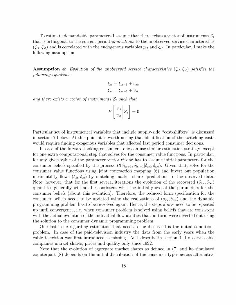
To estimate demand-side parameters I assume that there exists a vector of instruments Ztthat is orthogonal to the current period innovations to the unobserved service characteristics(ξct, ξst) and is correlated with the endogenous variables pct and qct. In particular, I make thefollowing assumption

Assumption 4: Evolution of the unobserved service characteristics (ξct, ξst) satisfies thefollowing equations

ξct = ξct−1 + vct,

ξst = ξst−1 + vst

and there exists a vector of instruments Zt such that

E

[vct

vst

∣∣∣∣∣Zt]

= 0

Particular set of instrumental variables that include supply-side “cost-shifters” is discussedin section 7 below. At this point it is worth noting that identification of the switching costswould require finding exogenous variables that affected last period consumer decisions.

In case of the forward-looking consumers, one can use similar estimation strategy exceptfor one extra computational step that solves for the consumer value functions. In particular,for any given value of the parameter vector Θ one has to assume initial parameters for theconsumer beliefs specified by the process P (δict+1, δist+1|δict, δist). Given that, solve for theconsumer value functions using joint contraction mapping (6) and invert out populationmean utility flows (δct, δst) by matching market shares predictions to the observed data.Note, however, that for the first several iterations the evolution of the recovered (δict, δist)quantities generally will not be consistent with the initial guess of the parameters for theconsumer beliefs (about this evolution). Therefore, the reduced form specification for theconsumer beliefs needs to be updated using the realizations of (δict, δist) and the dynamicprogramming problem has to be re-solved again. Hence, the steps above need to be repeatedup until convergence, i.e. when consumer problem is solved using beliefs that are consistentwith the actual evolution of the individual flow utilities that, in turn, were inverted out usingthe solution to the consumer dynamic programming problem.

One last issue regarding estimation that needs to be discussed is the initial conditionsproblem. In case of the paid-television industry the data from the early years when thecable television was first introduced is missing. As I describe in section 4, I observe cablecompanies market shares, prices and quality only since 1992.

Note that the evolution of aggregate market shares as defined in (7) and its simulatedcounterpart (8) depends on the initial distribution of the consumer types across alternative

18

services, i.e. (si,1992), ∀i. In order to obtain a guess about the initial distribution I assumethat prior to 1992 there were no paid television. Further, I assume that in 1992 consumersface only two alternatives, i.e. cable and over-the-air television. Given that DBS companieseffectively entered the market in 1993 I add the satellite alternative in 1993. Given that theinitial distribution of consumer types was approximated in this way, I use data from 1992 till1996 only to simulate initial conditions for the years 1997-2002.11 The hope is that by 1997variation in the cable and satellite prices and qualities alleviates the impact of the initialconditions assumption and the distribution of the consumer types across alternatives is closeto the true one.

6.2 Supply side

Parameters of the supply side can be estimated using generalized instrumental variablesapproach to the nonlinear rational expectations model developed in Hansen and Singleton(1982). In particular, define the following functions

gp(st−1, xt, pct, qct, st, xt+1) =∂Π(st−1, xt, pct, qct)

∂pct+ β

[∂st∂pct

]TEt

[∂W (st, xt+1)

∂st

](16)

gq(st−1, xt, pct, qct, st, xt+1) =∂Π(st−1, xt, pct, qct)

∂qct+ β

[∂st∂qct

]TEt

[∂W (st, xt+1)

∂st

](17)

Rational expectations assumption suggests that the following must be true

Et[gp(st−1, xt, pct, qct)] = 0 (18)

Et[gq(st−1, xt, pct, qct)] = 0 (19)

when evaluated at the observed (supposedly optimal) choices of the dynamic controls (pct, qct).12

There are several issues to consider. First, to construct empirical versions of gp(·) and gq(·)I need to know vector (st−1, xt, pct, qct). One possibility to proceed is to use the estimates ofthe consumer types distribution, st, and unobserved service characteristics (ξct, ξst) obtainedfrom the demand side.13

11There is another reason to omit data prior to 1997. Satellite penetration rates by DMA are availableonly from 1997. To backcast the satellite shares by market in 1993-1996 I used national-level dynamics insatellite shares and their values in 1997.

12Note that if policy functions are known exactly the conditions above must be equal to zero when evaluatedat observed price and quality choices, i.e. the model “overfits” the data. In estimation, however, wheneverpossible, I use observed realizations of the stochastic variables in the vector xt and simulate their evolutiononly after the terminal period in the data. This, in turn, generates deviations from the first-order conditions.In the new version of the paper I propose a way to introduce supply-side unobservables in a structural way.

13Note that computation of the standard errors for the supply side parameters in this case should accountfor the “first-stage” demand side estimation.

19

Second, constructing GMM estimator using (18) and (19) requires knowledge of a vector of

partial derivatives of the value function with respect to the state vector, i.e.

[∂W (st, xt+1)

∂st

].

This task is more challenging as it is not possible to express the derivatives in terms ofthe model primitives as it is often done in the literature on empirical Euler equations. Toovercome the problem I suggest using simulation technique in the spirit of Hotz et al. (1994)and Bajari et al. (2007).

First, I estimate policy functions p(st−1, xt) and q(st−1, xt) using the data, estimates ofthe distribution of consumer shares, and estimates of the evolution of exogenous variables xtobtained from the demand side.

Then I simulate forward NS possible paths (each of T periods length) of exogenous vari-ables, resulting policies and implied transitions of the endogenous variables. By computingsequences of the reward functions for each period and averaging over NS simulations I canget an approximation to the continuation value for any given starting point (st−1, xt).

In particular, let p(st−1, xt; θ) and q(st−1, xt; θ) denote parametric estimates of the policyfunctions. Then an approximation to the value function from following policies p(st−1, xt; θ)and q(st−1, xt; θ) is given by

W (st−1, xt) =1

NS

NS∑n=1

T∑t=0

βtΠ(st−1, xt, pct(st−1, xt), qct(st−1, xt)) (20)

and implied transition of the endogenous variables st = s(st−1, pct(st−1, xt), pct(st−1, xt)).Consider two perturbations to the vectors of states st−1 + ειj and st−1 − ειj where ιj is a

vector of dimension dim(st−1)× 1 with 1 in position j and zeros everywhere else. Then thederivative of value function with respect to a state variable j can be approximated as

∂W (st−1, xt)

∂sjt−1

=W (st−1 + ειj, xt)− W (st−1 − ειj, xt)

2ε(21)

In a similar way I can obtain approximations to derivatives with respect to each elementof st−1. Note that this is still a very computationally intense procedure because I need tosimulate dim(st−1) derivatives for each point in the data.

As it is pointed out in Bajari et al. (2007), significant saving in terms of computationtime comes from linearity of the reward function in the parameters of interest. In particular,if per-period reward function can be written as

Π(st−1, xt, pct, qct; θ) = Ψ(st−1, xt, pct, qct) · θ

where Ψ(st−1, xt, pct, qct) is an M−dimensional vector of basis functions, the computationallyintensive approximation of partial derivatives of the value function needs to be performedonly once. Then for every trial value of the parameter vector I can use the same basisfunctions previously stored in the memory.

20

In particular, suppose that the cost of providing quality qct per subscriber has the followingparametric representation

c(qct) = θ0 + θ1qct + θ2q2ct + θ3Z1ct + · · ·+ θK+2ZKct (22)

where θ3 through θK+2 are parameters for K cost shifters, Z1ct, . . . , ZKct.Then I can write

Π(st−1, xt, pct, qct) =N∑i=1

sic(sit−1, xt, pct, qct)pct −N∑i=1

sic(sit−1, xt, pct, qct) · θ0

−N∑i=1

sic(sit−1, xt, pct, qct)qct · θ1 −N∑i=1

sic(sit−1, xt, pct, qct)q2ct · θ2

−N∑i=1

sic(sit−1, xt, pct, qct) · Z1ctθ3 · · · −N∑i=1

sic(sit−1, xt, pct, qct) · ZKctθK+2

Define

Ψ1(st−1, xt, pct, qct) =1

NS

NS∑n=1

T∑t=0

βtN∑i=1

sic(sit−1, xt, pct, qct)pct

Ψ2(st−1, xt, pct, qct) =1

NS

NS∑n=1

T∑t=0

βtN∑i=1

sic(sit−1, xt, pct, qct)

Ψ3(st−1, xt, pct, qct) =1

NS

NS∑n=1

T∑t=0

βtN∑i=1

sic(sit−1, xt, pct, qct)qct

Ψ4(st−1, xt, pct, qct) =1

NS

NS∑n=1

T∑t=0

βtN∑i=1

sic(sit−1, xt, pct, qct)q2ct

Ψ5(st−1, xt, pct, qct) =1

NS

NS∑n=1

T∑t=0

βtN∑i=1

sic(sit−1, xt, pct, qct)Z1ct

. . .

ΨK+4(st−1, xt, pct, qct) =1

NS

NS∑n=1

T∑t=0

βtN∑i=1

sic(sit−1, xt, pct, qct)ZKct

Let ψjk =Ψk(st−1 + ειj, xt, pct, qct)−Ψk(st−1 − ειj, xt, pct, qct)

2ε, k = 1, . . . , K + 4. Then

approximation to the derivatives of value function can be computed as follows

∂W (st−1, xt)

∂sjt−1

= ψj1 − ψj2θ0 − ψj3θ1 · · · − ψjK+4θK+2

21

where the values of the basis functions are computed once and stored in memory. As longas all necessary basis functions are computed and stored in the computer memory they neednot be re-computed for each trial value of the supply side parameters.

7 Instruments and identification

According to the assumption 3, cable companies observe realizations of (pst, qst, ξst, ξct, Zct)prior to making their price and quality choices. Therefore, price and quality variables areclearly correlated with both the level of unobserved service characteristics and the currentperiod innovations to them. In order to find instruments for the demand-side estimation Iuse the following arguments.

First, possible instruments for price and quality levels of cable providers are averageprices and quality levels of other cable systems that belong to the same multiple-system-operator (MSO). These variables must be uncorrelated with the unobserved local marketservice characteristics, ξ’s, but should be reasonable proxies for the price and quality levelsoffered by the local cable system. Correlation in prices and quality levels across systemsoccurs because the owner of several cable systems typically negotiates programming fees andother contract arrangements with programming networks on behalf of all of its memberssimultaneously. In turn, correlation in the marginal costs of systems within the same MSOjustifies correlation in their price and quality levels. For the instruments to be valid, one mustensure that the unobserved demand shocks, ξ’s are not correlated across the systems. It isless obvious because MSO typically own geographically concentrated firms. If unobserveddemand shocks are closely correlated across different cable markets, the validity of theseinstruments may be questionable.

Second, different MSO’s have different bargaining power in negotiations with program-ming networks. It is conceivable that larger MSO’s with bigger number of subscribers totheir cable systems have stronger bargaining position. Hence, I used the number of MSOsubscribers as another instrument that shifts costs of all its members.

Third, programming networks often sell bundles consisting of several channels. Ability topurchase such bundles depends on the capacity level (in terms of the maximum number ofchannels physically possible to transmit through the cable system). Hence, average capacitylevel within MSO should be correlated with the ability of their member-systems to get lowerrates. By the same logic, I used own capacity level as another instrumental variable. Itis possible that systems with more favorable innovations into their ξct would have highermarginal profitability of capital and, hence, would invest more actively into own systemcapacity. However, it is less likely that the system’s capacity level would immediately respondto the current period innovation.

Fourth, total length of own coaxial lines of the local cable systems is a proxy for thedifferences in maintenance costs incurred by the systems in areas with different densities of

22

houses.Fifth, by exploiting peculiarities of the paid-television industry where satellite companies

set their prices and quality at the national level I can use pst and qst as instruments forlocal cable price and quality variables. The argument here is that DBS prices and qualityare not likely to respond to changes in the local demand unobservables (ξct, ξst), while cablecompanies choose price and quality locally after observing realizations of pst and qst.

14

So far I described instruments used to solve the problem of price and quality endogene-ity. Given that the model has extra parameters for the distribution of switching costs, itis necessary to discuss the instruments that help to identify them. Non-trivial switchingcosts generate state dependence in consumer utility. Loosely speaking, switching costs are“coefficients” on the lagged market shares if we were running linear regression. Exogenousvariables that were relevant for the previous period consumer choices should serve as infor-mative additional instruments to identify consumer switching costs. Therefore, in additionto the current period values of the instrumental variables discussed above I included theirlagged values.

Finally, I used another set of IV’s that should enhance identification of the switching costsparameters.15 Moving decisions are likely to exogenously “reset” last period consumer statemore often in the regions with high population mobility. To proxy for population mobility Iused the number of housing permits issued at the state level.

Up until recently, in order to install satellite dish in a multy-story buildings consumershave to obtain a permission from the owner, which complicated usage of the satellite televisionin regions with a large number of multiunit buildings. This motivates including variables likepercentage of dwelling units in multiunit structures of 5 or more units.16

Another complication that many satellite subscribers face is related to the “southernexposure” issue, i.e. the necessity to locate the receiver (dish) in a place that guaranteesopen access to the orbital satellite. To control for the geographic location of a particularmarket I used its longitude and latitude as two extra instruments.

8 Estimation results

In this section I present preliminary results for the demand and supply side estimation.Demand side parameters were estimated using GMM based on a sample of 564 local cable

14A problem may arise if the unobserved service characteristics or, more generally, demand-side unobserv-ables (ξct, ξst) are correlated across markets and are taken into considerations by the satellite providers.

15Note that some of these IV’s are not explicitly in the model. Some of them are easy to explicitlyincorporate into a myopic consumer model than into the dynamic one. In the future versions of the paper Idevote more space to discussing such possibilities.

16Also, it is conceivable that serving multiunit building is cheaper for a cable company than serving anequivalent number of separate houses.

23

markets in 1992-2002. Due to the data limitations discussed in section 6.1, to form theempirical moment conditions I used data from 1997-2002.

Given parameter estimates of the demand side, I augmented observed data with theestimates of the unobserved service characteristics of cable and satellite services and estimatedparameters of the cost function for the supply-side model.17

8.1 Demand side

Demand side structural parameters were estimated using assumption of consumer myopia. Tocontrol for persistent consumer heterogeneity I used 30 consumer types whose preferences arerepresented by the iid draws from a normal distribution with a diagonal variance-covariancematrix. Table 3 presents results of the random coefficients model.

Table 3: 30-types model estimation results, GMMVariable 1st stage 2nd stage

Switching cost (cab) 0.949 1.151(s.e.) (0.521) (0.591)σηc 9.23e-05 8.03e-05(s.e.) (40.98) (48.16)Switching cost (sat) 2.238 1.844(s.e.) (0.370) (0.442)σηs 0.0001 7.95e-05(s.e.) (29.44) (32.75)σconstc 4.03e-05 3.33e-05(s.e.) (38.42) (40.49)σconsts 9.02e-05 9.66e-05(s.e.) (2.737) (3.442)Price coefficient -0.047 -0.087(s.e.) (0.008) (0.010)σηp 1.38e-06 1.42e-06(s.e.) (0.370) (0.435)Quality coefficient 0.072 0.051(s.e.) (0.011) (0.011))F-value:

Note that none of the parameters of consumer heterogeneity were precisely estimated.Point estimates of the standard deviations for the switching costs and constant term pa-

17Note that standard errors for the supply side parameters do not account for the first stage demandestimation. Necessary adjustment will be made in the next version of the paper.

24

rameters are fairly close to zero. The same is true for the standard deviation of the pricecoefficient. Standard errors are huge for all of the standard deviations.

On the other hand, the levels of switching costs as well as price and quality coefficients areestimated precisely. Note that since moment conditions were constructed using innovationsinto the unobserved service characteristics (ξct, ξst), i.e. the latter ones were first-differenced,any constant terms in the mean utility specification are not separately identified from themeans of the unobservables.

Given that the data fails to reject a representative consumer model, I re-estimated thedemand side model under assumption of one consumer type. The results are presented intable 4.

Table 4: One-type model estimation results, GMMVariable 1st stage 2nd stage Cont. updated

Switching cost (cab) 0.949 1.036 1.171(s.e.) (0.488) (0.560) (0.571)Switching cost (sat) 2.238 1.844 1.868(s.e.) (0.230) (0.294) (0.301)Price coefficient -0.047 -0.087 -0.094(s.e.) (0.005) (0.005) (0.006)Quality coefficient 0.072 0.051 0.046(s.e.) (0.005) (0.005) (0.005)F-value: 67.8 452.8 339.9

The level of consumer switching costs for cable and satellite providers was estimated at$149 and $238 respectively.18

8.2 Supply side

In order to augment the data for estimation of the parameters of the cable companies costfunction I use fitted values of the unobserved quantities (ξct, ξst) obtained from the demandside estimates. Since parameters of the consumer heterogeneity have point estimates close tozero and are not statistically significant at any reasonable significance level, the distributionof consumer heterogeneity collapses to a simple mean market shares for cable and satellite.

As discussed in section 6.2, to estimate parameters of the cable companies cost function

18These estimates are slightly higher than the ones obtained from the dynamic demand specification. Inanother paper Shcherbakov (2008) I find that cable and satellite switching costs were approximately $109and $186. The difference in the estimates can be attributed to both the differences in the model frameworkand the differences in the data used for estimation.

25

I first estimated policy functions

pct = p(st−1, xt; θ)

qct = q(st−1, xt; θ)

where xt includes satellite price and quality, average MSO price and quality, own and MSOcapacity levels, miles of coaxial cable (in thousands), the number of MSO subscribers (inthousands), last period market shares, and the estimates of the unobserved cable and satelliteservice characteristics. The estimation results can be found in Appendix 1.

I used the estimated policy functions to simulate 1,000 sequences of 500 periods each toestimate basis functions for the numerical derivatives approximation. For the preliminaryestimation I assumed that all of the exogenous state variables with the exception of unob-served service characteristics (ξct, ξst) evolve deterministically till the terminal period in thedata and then stay constant forever. This is a very strong assumption and at the moment Iam working on a long-run model of the cable firms behavior that would allow for investmentand stochastic evolution of the cost shifters.

The evolution of the exogenous variables (ξct, ξst) is assumed to satisfy a random walkassumption with simulated innovations drawn from normal distribution with the varianceequal to the empirical variance of the observed innovations. Conditional on the currentsimulated realizations of the cable and satellite unobservables I predict policies (pct, qct) andupdate current values of the endogenous variables (sct, sst).

To estimate parameters of the cable companies cost function I use moment conditionsspecified in (18) and (19). The set of instruments includes own price and quality levels, priceand quality of satellite companies, and the entire set of cost shifters. Preliminary estimationresults are listed in table 5.

According to the estimates of the cable cost function, per-subscriber costs of providingservice is increasing in the quality level at a slightly increasing rate.

Most of the coefficients on the cost shifters are statistically significant and have expectedsigns. In particular, the cost is increasing in average MSO price and decreasing in averageMSO quality, which is consistent with the intuition behind this cost shifter. Cost of providingtelevision service is decreasing in own capacity level. This suggests non-trivial gains tohigh capacity levels that allow for cost reduction when purchasing bundles of programmingnetworks rather than individual channels.

Coefficient on the own length of coaxial lines is positive though not statistically significant.Unexpectedly, average MSO capacity level seems to have significant positive effect on the owncost structure of cable providers.

Finally, the average number of MSO subscribers tends to reduce costs of the cable com-panies.

Current estimates of the cable cost function suggest that the average level of costs wasabout $2.19 (median $2.12) per subscriber with the average price-cost margins of about

26

Table 5: Supply-side model, GMMDynamic producer Myopic producer

Variable First stage Second stage First stage Second stageConst. -14.1270 -14.9800 -18.6780 -19.0230(s.e.) (0.8157) (0.8011) (1.0816) (1.0865)qc 0.4884 0.4916 0.4770 0.4884(s.e.) (0.0006) (0.0001) (0.0011) (0.0003)qc2 0.0021 0.0005 0.0042 0.0011(s.e.) (0.0001) (0.0000) (0.0002) (0.0000)MSO(pc) 1.0514 1.0412 1.0002 0.9810(s.e.) (0.0216) (0.0213) (0.0312) (0.0317)MSO(qc) -0.5124 -0.6250 -0.8816 -1.0590(s.e.) (0.0966) (0.0952) (0.1385) (0.1390)CAP -0.0992 -0.1006 -0.1110 -0.1193(s.e.) (0.0084) (0.0083) (0.0134) (0.0137)MCOAX 0.4738 0.0450 -0.1892 -0.0125(s.e.) (0.3378) (0.3573) (0.7165) (0.7198)MSO(CAP ) 0.0220 0.0691 0.0790 0.1109(s.e.) (0.0170) (0.0165) (0.0233) (0.0236)MSO(SUB) -0.1019 -0.1085 -0.1806 -0.2094(s.e.) (0.0176) (0.0172) (0.0269) (0.0278)F-value 365.9 403.5 482.6 439.66

$16.52 (median $16.42). Interestingly, in some cases the estimates suggest negative price-cost margins of as low as $-3.04 per subscriber. Unless the negative estimates is an artifactof incorrectly specified supply and demand models, this suggests importance of dynamicprice and quality policies, when producers invest heavily into the customer base by usingintroductory pricing in the initial periods.

The myopic model estimates (i.e. when discount factor on the continuation value was setto zero), suggests that the average level of costs is -$4.14 (median -$3.77). The price-costmargin is estimated at the mean level of $22.85 (median $22.65). Hence, the estimates fromthe myopic model are less plausible given the data on average prices in cable industry.

9 Counterfactual simulations

In this section I provide two counterfactual simulations that rely on the preliminary demandand supply side estimates. The first scenario evaluates the effect of switching costs on thecable television prices under assumption that prices and quality levels of the satellite company

27

as well as own cost structure of the cable providers do not change. This outcome correspondsto a static duopoly model. The second scenario calculates new prices under no-satellite-no-switching-costs assumption, i.e. a static monopoly model.

Before discussing the results of the counterfactual simulations it is worth noting one pecu-liarity of a representative consumer model with linear consumer utility function. Consider ageneral formulation of the producer dynamic programming problem where demand scheduleis given by myopic consumers who nevertheless face significant switching costs.19

W (sct−1, sst−1, xct) = maxpct,qct

s(sct−1, sst−1, xct, pct, qct)(pct − c(qct, Zct)) + βEW (sct, sst, xct+1)

Since consumer utility is linear in price and quality, there exists a well defined inverse

p = δ−1(δct, qct, ξct).

Moreover,∂δ−1(δct, qct, ξct)

∂qctis constant. Note also that conditional on δct, if there are no

adjustment costs for (pct, qct), particular choices of (pct, qct) do not have dynamic implications.Therefore, producer problem can be written as

W (sct−1, sst−1, xct) =

maxδct,qct

s(sct−1, sst−1, xct, δct)(δ

−1(δct, qct, ξct)− C(qct, Zct) + βE[W (sct, sst, xct+1)]

From the first order conditions for optimal quality choice (given δct),

FOC[qct] :∂δ−1(δct, qct, ξct)

∂qct− ∂C(qct, Zct)

∂qct= 0

where the first term is constant due to the linearity of the utility function it is clear thatq∗ct = q(ξct, Xct) does not depend on the optimal choice of a dynamic control, δct.

The main implication of the discussion above is that if the vector of cost shifters Zct doesnot change across counterfactual simulations the optimal choice of quality will not changeas well. Hence, changes in the market structure due to elimination of switching costs wouldaffect only cable price. Note that this is an artifact of both the representative consumermodel assumption and the linearity of the consumer per-period utility. For example, theargument would not work for a random coefficients demand side model.

Since according to the preliminary demand estimates the data does not reject a represen-tative consumer model I simulate counterfactual scenarios using this model.

In order to calculate new cable prices I numerically solve static first order conditionsfor cable company where cost function is evaluated at observed vector of cost shifters and

19The same argument goes through in case if consumers are boundedly rational and forecast future flowutility using its current values only.

28

quality choices. The results of the counterfactual simulations suggest that in a static duopolyscenario with the unchanged satellite policy and the same vector of cable cost shifters averagecable prices would be $24.59, which is 28 percent higher than the observed average price. Incase of a static monopoly scenario average cable price is $28.90, which is about 51 percenthigher than the observed value of $19.20.

10 Conclusions

This paper addresses questions about the effects of consumer switching costs on the marketstructure and social welfare. Answers to these questions depend critically on the ability toestimate supply side parameters in presence of state dependent utility on the demand side.Multiple consumer types and/or products result in a state space that is too large to makenumerical solution to the producer dynamic programming problem computationally feasible.

To overcome this problem I suggest to estimate supply side parameters from the optimal-ity conditions for dynamic controls. In case when one dynamic control shifts several statevariables at the same time it is very hard to derive an Euler equation in terms of the modelprimitives. However, there is a computationally feasible alternative that relies on simulationof the derivatives of the value function with respect to the state variables. Under the ratio-nal expectations assumption dynamic first order conditions could be used to form momentconditions for estimation.

The problem of unobserved distribution of consumer types across market shares andunobserved service characteristics is solved by first estimating the demand relationship andrecovering the desired variables.

Preliminary estimates of the demand side parameters suggest switching costs of $149 and$238 for cable and satellite providers respectively. The demand side estimates cannot rejecta representative consumer model, although mean levels of switching costs as well as price andquality coefficients are estimated precisely. Supply-side estimates imply the average cost ofproviding service per subscriber of about $2.19 and average price-cost margin of $16.52 permonth.

Counterfactual simulations suggest that without switching costs in a duopoly situationaverage cable prices would be about $24.59, which is 28 percent higher than the observedaverage prices of $19.20. In case if there are no switching costs on the demand side and thereare no satellite competitor (i.e. static monopoly scenario) average cable prices are estimatedto be about $28.90, which is 51 percent percent higher than the observed ones.

References

Bajari, P., Benkard, L., and Levin, J. (2007). Estimating dynamic models of imperfectcompetition. Econometrica, 75(5):1331–1370.

29

Berry, S., Levinsohn, J., and Pakes, A. (1995). Automobile prices in market equilibrium.Econometrica, 63:841–890.

Berry, S. and Pakes, A. (2001). Estimation from the optimality conditions for dynamiccontrols. Unpublished manuscript. Yale University.

Borenstein, S. (1992). The evolution of u.s. airline competition. The Journal of EconomicPerspectives, 6:45–73.

Che, H., Sudhir, K., and Seetharaman, P. (2006). Bounded rationality in pricing under statedependent demand: do firms look ahead? how far ahead? Unpublished manuscript. YaleSchool of Management.

Chu, C. S. (2007). The effect of satellite entry on product quality for cable. Unpublisheddissertation, Stanford University.

Dube, J.-P., Hitsch, G., Rossi, P., and Vitorino, M. (2008). Category pricing with state-dependent utility. Marketing Science, 27(3):417–429.

FCC (2000). Fact sheet. Cable television infromation bulletin. FederalCommunications Commission, 445 12th Street, S.W., Washington, D.C.http://www.fcc.gov/mb/facts/csgen.html (accessed March 01, 2009).

Gowrisankaran, G. and Rysman, M. (2007). Dynamics of consumer demand for new durablegoods. Unpublished manuscript, University of Arizona.

Hansen, L. and Singleton, K. (1982). Generalized instrumental variables estimation of non-linear rational expectations models. Econometrica, 50(5):1269–1286.

Ho, C.-Y. (2009). Switching cost and the deposit demand in China. Unpublished manuscript.Georgia Institute of Technology.

Hotz, J., Miller, R., Sanders, S., and Smith, J. (1994). A simulation estimator for dynamicmodels of discrete choice. The Review of Economic Studies, 61(2):265–289.

Israel, M. (2003). Consumer learning about established firms: evidence from automobileinsurance. Working Paper 0020, The Center for the Study of Industrial Organization atNorthwestern University.

Kim, M., Kliger, D., and Vale, B. (2003). Estimating switching costs: the case of banking.Journal of Financial Intermediation, 12:25–56.

Kiser, E. (2002). Predicting household switching behavior and switching costs at depositoryinstitutions. Review of Industrial Organization, 20:349–365.

30

Knittel, C. (1997). Interstate long distance rates: search costs, switching costs and marketpower. Review of Industrial Organization, 12:519–536.

Krusell, P. and Smith, A. (1998). Income and wealth heterogeneity in the macroeconomy.The Journal of Political Economy, 106(5):867–896.

Melnikov, O. (2001). Demand for differentiated durable products: the case of the U.S.computer printer market. Unpublished manuscript, Cornell University.

Salies, E. (2005). A measure of switching costs in the GB electricity retail market. WorkingPaper 2005-9, GRJM.

Schiraldi, P. (2006). Automobile replacement: a dynamic structural approach. Job MarketPaper, Boston University.

Sharpe, S. (1997). The effect of consumer switching costs on prices: a theory and its appli-cation to the bank deposit market. Review of Industrial Organization, 12:79–94.

Shcherbakov, O. (2008). Measuring consumer switching costs in the television industry.Unpublished manuscript, University of Arizona.

Shy, O. (2002). A quick-and-easy method for estimating switching costs. InternationalJournal of Industrial Organization, 20:71–87.

Sturluson, J. (2002). Consumer search and switching costs in electricity retailing. Ph.D. the-sis, Chapter 1, in Topics in the Industrial Organization of Electricity Markets, StockholmSchool of Economics, Sweden.

Appendix 1. Estimates of the policy functions

31

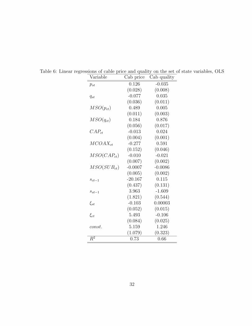
Table 6: Linear regressions of cable price and quality on the set of state variables, OLSVariable Cab price Cab quality

pst 0.126 -0.035(0.028) (0.008)

qst -0.077 0.035(0.036) (0.011)

MSO(pct) 0.489 0.005(0.011) (0.003)

MSO(qct) 0.184 0.876(0.056) (0.017)

CAPct -0.013 0.024(0.004) (0.001)

MCOAXct -0.277 0.591(0.152) (0.046)

MSO(CAPct) -0.010 -0.021(0.007) (0.002)

MSO(SUBct) -0.0007 -0.0086(0.005) (0.002)

sct−1 -20.167 0.115(0.437) (0.131)

sst−1 3.963 -1.609(1.821) (0.544)

ξst -0.103 0.00003(0.052) (0.015)

ξct 5.493 -0.106(0.084) (0.025)

const. 5.159 1.246(1.079) (0.323)

R2 0.73 0.66

32