the dynamics of systems of deformable bodies - pure · the dynamics of systems of deformable bodles...
TRANSCRIPT

The dynamics of systems of deformable bodies
Koppens, W.P.
DOI:10.6100/IR297020
Published: 01/01/1989
Document VersionPublisher’s PDF, also known as Version of Record (includes final page, issue and volume numbers)
Please check the document version of this publication:
• A submitted manuscript is the author's version of the article upon submission and before peer-review. There can be important differencesbetween the submitted version and the official published version of record. People interested in the research are advised to contact theauthor for the final version of the publication, or visit the DOI to the publisher's website.• The final author version and the galley proof are versions of the publication after peer review.• The final published version features the final layout of the paper including the volume, issue and page numbers.
Link to publication
General rightsCopyright and moral rights for the publications made accessible in the public portal are retained by the authors and/or other copyright ownersand it is a condition of accessing publications that users recognise and abide by the legal requirements associated with these rights.
• Users may download and print one copy of any publication from the public portal for the purpose of private study or research. • You may not further distribute the material or use it for any profit-making activity or commercial gain • You may freely distribute the URL identifying the publication in the public portal ?
Take down policyIf you believe that this document breaches copyright please contact us providing details, and we will remove access to the work immediatelyand investigate your claim.
Download date: 24. Aug. 2018

THE DYNAMICS OF SYSTEMS
OF DEFORMABLE BODlES
W. P. KOPPENS

THE DYNAMICS OF SYSTEMS
OF DEFORMABLE BODlES

ISBN 90-9002579-0
printed by krips repro meppel
THE DYNAMICS OF SYSTEMS
OF DEFORMABLE BODlES
PROEFSCHRIFT
ter verkrijging van de graad van doctor aan
de Technische Universiteit Eindhoven, op gezag
van de Rector Magnificus, prof. ir. M. Tels,
voor een commissie aangewezen door het College
van Dekarren in het openbaar te verdedigen op
dinsdag 31 januari 1989 te 16.00 uur
door
WILHEL~1US PETRUS KOPPENS
geboren 1 september 1957 te Deurne

Dit proefschrift is goedgekeurd door de promotor:
prof. dr. ir. D.H. van Campen
copromotor:
dr. ir. A.A.H.J. Sauren

Preface
This research was conducted at the sectien of Fundamentals of Mechanica!
Engineering, faculty of Mechanica! Engineering, Eindhoven University of
Technology. It was supervised by Dr. Fons Sauren and professor Dick van Campen.
During informal discussions I received valuable comments of memhers of the
sectien of Fundamentals of Mechanica! Engineering. Especially the comments of
Dr. Frans Veldpaus on the theoretica! part presented in chapter 2 are
acknowledged. As part of their thesis work, Ir. Alex de Vos, Ir. Peter Deen, Ir.
Edwin Starmans, Ir. André de Craen and Ir. Paul Lemmen participated in this
research. I thank everybody especially for the many discussions we had. These
made me carry out this research with pleasure. Further I want to express my
appreciation to Dr. Harrie Rooijackers for helping me with several computer
problems.
Finally I express my appreciation to Computer Aided Design Software, Inc.
(CADSI), Oakdale, Iowa, for providing the souree code of some of the subroutines
of DADS which I required for doing several of the investigations presented in this
thesis.
Deurne, November 1988 Willy Koppens
V
Table of contents
PREFACE v
ABSTRACT ix
1 INTRODUCTION 1
2 THE EQUATIONS OF MOTION OF A DEFORMABLE BODY 7
2.1 Introduetion 7
2.2 The kinematics of a deformable body 7
2.3 The equations of motion of a deformable body 11
2.4 Approximate equations of motion: Galerkin's method 14
2.5 Approximate equations of motion in component form
3 GENERATING BASE FUNCTIONS
3.1 Introduetion
3.2 Assumed-modes method
3.3 Fini te element method
3.4 Modal synthesis method
17
20
20 20 25
34
'1 THE EQUATIONS OF MOTION OF A SYSTEM OF BODlES 36
4.1 Introduetion
4.2 Energetic and active connections
4.3 Kinematic connections
4.4 The equations of motion of a system of bodies
4.4.1 The global description
4.4.2 The relative description
36
37
38 42
43
45
5 ASSESSMENT OF DESCRIPTIONS AND APPROXIMATIONS 48
5.1 Introduetion
5.2 Mean displacement conditions
5.3 The finite element method
48
48
52
vii

5.4 The modal synthesis method 57
5.4.1 Selection of base functions 57
5.4.2 Elimination of rigid body motions 62
5.4.3 Lumped mass approximation 65
5.5 Nonlinearities corresponding to displacements due to deformation 66
5.5.1 Nonlinear strain-displacement relations 67
5.5.2 Nonlinear combinations of assumed displacement fields 68
5.6 Shifting of frequencies 71
5.6.1 Tuning of frequencies 71
5.6.2 Lowering of high frequencies 74
6 CONCLUDING REMARKS 76
6.1 Conclusions
6.2 Suggestions for further research
REPERENCES
APPENDICES
A MATHEMATICAL NOTATION
B DESCRIPTION OF ROTATIONAL MOTION IN TERMS OF EULER
PARAMETERS
C BEAM ELEMENT
76
77
79
85
89
92
D ELASTODYNAMIC ANALYSIS OF A SLIDER"CRANK MECHANISM 96
SAMENVATTING 99
viii

Abstract
In this thesis, a mathematica! description is presented of the dynamic behaviour of
systems of interconnected deformable bodies.
The displacement field of a body is resolved into a displacement field due to a
rigid body motion and a displacement field due to deformation. In order to get an
unambiguous resolution, the displacement field due to deformation is required to be
such that it cannot represent rigid body motions. This is achieved by prescrihing
either displacements due to deformation of selected particles or mean displacements
due to deformation.
Starting from the equations of motion of a partiele of the body, a variational
formulation of the equations of motion of the free body is derived. These equations
are simpler in case the mean displacements due to deformation are equal to zero.
Approximate equations of motion are obtained by approximating the displacement
field due to deformation by a linear combination of a set of assumed displacement
fields. Three methods are described for generating assumed displacement fields,
namely the assumed-modes method, the finite element method, and the modal
synthesis method.
For formulating the equations of motion of a body which forms part of a system
of bodies, the interconnections with other bodies must be accounted for. Energetic
and active connections can betaken into account by adding the forces they generate
to the applied forces on the free body. Kinematic connections constrain the relative
motion of interconnected bodies. This can be accounted for with constraint
equations, that can be used for partitioning the variables that describe the
kinematics of the system of bodies into dependent and independent variables. For
formulating constraint equations it is convenient to introduce variables that
describe the relative motion of the interconnected bodies.
The simplification of the equations of motion in case the mean displacements
due to deformation are chosen equal to zero, leads to a computation time reduction
of a few decades of per cents in the most favourable case. For the systems investi
gated in this thesis the dynamic behaviour is approximated better in case
displacement fields due to deformation are approximated by assumed displacement
fields with mean displacements equal to zero. Caution must be taken in preventing
rigid body motions of the displacement field due to deformation by prescrihing
displacementsof selected particles of the body, sirree this may result in an incorrect
ix

solution of the dynamic behaviour.
The assumed-modes method is only feasible for regularly shaped bodies. The
finite element method and the modal synthesis method can be used for boclies with
arbitrary shape. The finite element method leads often to a model with many
degrees of freedom. The solution of such a model requires much computation time.
The modal synthesis method can then be used with success to reduce the number of
degrees of freedom such that the required computation time is cut down. The
effectiveness of the modal synthesis method depends to a great extent on a proper
choice of the assumed displacement fields. Such a choice can generally be made in
advance on the basis of the load on the body. The lumped mass approximation,
which is frequently used in literature, is feasible for determining time-independent
mass coefficients from displacement fields which have been determined with a
standard finite element program. One should bear in mind that a finer subdivision
into elements may be required than would be necessary for determining the
displacement fields sufficiently accurate.
A method is proposed to improve approximations for descrihing the dynamic
behaviour of a body for a specific set of assumed displacement fields. This method
has been used successfully for reducing the required computation time by lowering
irrelevant high frequencies.
x

chapter 1
Introduetion
The increase in capacity of computers has opened the possibility to simulate the
dynamic behaviour of complex mechanica! systems, such as spacecraft and vehicles,
already in the design phase. This may save expensive modifications of prototypes
which wiJl be necessary in case the dynamic behaviour is inadequate. Increasing
demands on the dynan1ic behaviour and more flexible system parts due to a more
economical use of matcrials require that deformation of the parts is taken into
account in determining the dynamic behaviour.
Mechanica! systems differ in various ways, such as the number of bodies, the
types of connections joining the bodies, and the topology. Many papers with the
main objective to present a formalism to develop equations of motion for general
mechanica! systems have been published. Often the presented theory is restricted to
a specific class of mechanica! systems, such as systems with rigid boclies or
two-dimensional systems. A survey will be given of three important topics related
to the description of the dynamic behaviour of mechanica! systerns, namely the
description of the kinematics of mechanica! systems, mechanica! principles for
deriving the equations of motion, and deformability of bodies.
Two ways to describe the kinematics of mechanica! systems are in common use,
namely the global description and the relative description. In the global description,
the positions of all bodies are described relative to an inertial space. In deriving the
equations of motion, the kinematic connections between the bodies are taken into
account separately by means of eenstraint equations. The resulting equations of
motion are a set of mixed differential-algebraic equations having a simple form.
Special techniques are required for solving these equations. The global description is
used by, among others, Orlandea et al. (1977a, b), Wehage and Haug (1982), Hang
et al. (1986), and Changizi et al. (1986).
The finite element formulation presented by Van der Werff and Jonker (1984)
may be regarcled as a variant of the global description. They describe the position
and orientation of nodes relative to an inertial space. Both bodies and connections
are considered as finite elements. This allows to obtain the equations of motion of a
mechanica! system by a standard assembly process. The relative motion of nodes of
an element are described with deformation mode coordinates which are nonlinear
functions of the nodal displacements. When a relative motion is constrained, such
1

as may be the case for rigid bodies, the corresponding deformation coordinate
equals zero which leads to a constraint equation.
In the relative description, the position of one arbitrary body is described
relative to an inertial space; the positions of the other bodies are described relative
to a body whose position has already been described, in terms of variables
characterizing the relative motion. For systems without kinematically closed
chains, these variables are independent. The resulting equations of motion are a set
of differential equations of minimal dimension. In systems with kinematically closed
chains, the closed ebains are first opened by cutting the chains imaginarily. Then,
the kinematics can be described in terms of the variables which characterize the
relative motion of the bodies. Accounting for the cuts renders these variables
dependent. For some mechanica! systems with a simple geometrie configuration
only, this dependency can be eliminated. However, in general the resulting
equations will be too involved. Therefore, the dependency is usually taken into
account separately by means of constraint equations just as with the global
description. As compared with the global description, the number of constraint
equations going with the relative description is small; however, they involve the
kinematic variables of all the bodies in a closed chain whereas in the global
description only the kinematic variables of pairs of interconnected bodies are
involved. The resulting equations of motion are a set of mixed differential-algebraic
equations like with the global description. The relative description is used by,
among others, Wittenburg (1977), Ruston and Passerclio (1979), Sol (1983),
Schiehlen (1984), and Singh et al. (1985).
A combination of the global description and the relative description has been
presented by Haug and McCullough (1986). They derived the equations of motion
for recurring subsystems with a particular kinematic structure using the relative
description. Special purpose modules are used to evaluate these equations of
motion. The result is added to the equations of motion of the remairring part of the
system whose kinematics is described using the global description. They observed a
vastly improved computational efficiency as compared to a program based on the
global description (McCullough and Haug, 1986).
The second important item is the mechanica/ principle used for deriving the
equations of mot ion. Several papers (e.g. Schiehlen, 1981; Kane and Levinson, 1983;
and Koplik and Leu, 1986) deal with the question: Which mechanica! principle
yields equations of motion in the least tedious way and having the simplest form?
However, this is only anitem of argument when the relative description is used for
descrihing the kinematics of the mechanica! system, because some principles, for
2
example Lagrange's equations of motion, take the kinematics of the systern into
account from the start. When the global description is used, all mechanica!
principles yield without any trouble the equations of rnotion. In case the relative
description is used, a variational forrnulation is most suited, such as Lagrange's
form of d' Alembert's principle (Witten burg, 1977), Kane's method of generalized
speed (Kane, 1968), and Jourdain's principle (Schiehlen, 1986).
The third important item is the influence of deformability of bodies. Many
papers deal with the dynamic analysis of mechanica! systems that contain
deforrnable bodies. Most papers use the same description of the kinernatics of
deformable bodies: the displacernents of particles of a deformable body are resolved
into displacements due toa rigid body motion of the body and displacements due to
deformation of the body. This resolution is done in such a way that the strain
displacement relations rnay be linearized in case the strains are smal!. Further,
most papers use Galerkin's rnethod for obtaining an approximate solution of the
equations of motion in the space domain. This involves an expansion of the
displacements due to deformation of the body in a linear combination of linearly
independent displacement fields. The papers differ in the way these displacement
fields are generated: this is most often done by either the finite element method
(Song and Haug, 1980; Thompson and Sung, 1984; Turcic a.nd Midha, 1984a, b;
Van der Weeën, 1985) or the modal method (Sunada and Dubowsky, 1981, 198:3;
Yoo and Haug, 1986a, b, c; Agrawal and Shabana, 1985). The papers differ further
in the degree to which the coupling between rigid body motion and displacements
due to deforrnation is included. The most sirnple ana.lysis metbod considers only the
quasi-static deflection caused by the inertia forces due to the motion which follows
from a kinematic analysis of a conesponding rigid body model. Erdman and Sandor
(1972) refer to such an analysis as elastodynamic ana.lysis. In a more refined
analysis, the inertia contribution conesponding to the displacements caused by
deformation are also taken into account (Thompson and Sung, 1984; Turcic and
Midha, 1984a, b). The most refined analysis departs from unknown rigid body
rnotions and includes all coupling terms (Song and Haug, 1980; Sunada and
Dubowsky, 1981, 1983; Yoo and Haug, 1986a, b, c; Agrawal and Shabana, 198.5;
Van der Weeën, 1985; Lilov and Wittenburg, 1986; Koppens et al., 1988).
The subjects of difference and resemblance of the numerous papers on the
dynamics of systems of deformable bodies do not become clear from the literature.
It is the purpose of this thesis to give a unified description of the dynamics of
systerns of deformable bodies. From this description the various descriptions that
can be found in the literature can be derived. It is expected that this wil! increase
3

the insight into the various descriptions.
The dynamics of an individual deformable body is presented in chapter 2. The
displacements of the body are resolved into displacements · due to deformation and
displacements due to a rigid body motion. The order in which the displacements of
the body are resolved is opposite to the usual order. This provides that the rotation
tensor that describes the rigid body motion can be readily factored out of the
deformation tensor, and that there is no need to introduce time differentiation of
the displacements due to deformation relative to a rotating frame. However, the
order of this resolution is immaterial for the ultimate equations of motion. The
resolution of displacements of the body is ambiguous. Conditions are imposed on
the displacement field due to deformation in order to get a unique resolution. Two
types of conditions are described, namely conditions on displacements of selected
material points of the body and conditions on the mean displacementsof the body.
Starting from the equations of motion of a partiele of the body, a variational
formulation for the equations of motion of the body is derived. lt is shown that the
equations of motion become considerably simpler when the displacements due to
deformation satisfy the conditions on the mean displacements of the body. The
equations of motion contain partial derivatives with respect to material
coordinates. In general, such equations admit no closed-form solution. In view of
this, approximate equations of motion are derived u&ing Galerkin's method. This
involves approximating the displacements due to deformation as a linear combina
tion of assumed displacement fields. The above description of the kinematics of the
body and the derivation of the equations of motion are done in terms of veetors and
tensors in their symbolic form. Finally, the ultimate equations of motion are
written in terms of the components of veetors and tensors relative to an
orthorrormal right-handed inertial base. It is shown that it is preferabie to write the
equations of motion in terms of the components of the angular velocity vector
above the more used first and second time derivatives of angular orientation
variables.
The most simple material behaviour is used namely isotropie linear elastic
material behaviour, because the emphasis of this thesis is on the description of the
dynamics of deformable bodies. Ho wever, anisotropic, nonlinear elastic, or visco
elastic material behaviour can be introduced without insurmountable difficulties by
introducing the proper constitutive relation.
In chapter 3, three procedures for generating assumed displacement fields for
approximating the displacements due to deformation are reviewed. The assumedmodes method can be used for regularly shaped bodies. The assumed displacement
4
fields are analytic functions of the material coordinates. It is limited in scope
because regularly shaped bodies are rare in practice. The finite element method is a
more versatile method. It consists of subdividing the body into regularly shaped
volumes. The displacements within such a volume can be easily approximated by
analytic functions. These are chosen such that compatibility of displacements of
neighbouring volumes can be easily ensured. However, the finite element metbod
generally leads to a model with many degrees of freedom. These can be reduced by
using a reduced set of linear combinations of finite element displacement fields.
This approach is known as the modal synthesis method. lt combines the versatility
of the finite element method and the efficiency of the assumed-modes method.
The equations of motion of a system of oodies are considered in chapter 4.
Boclies may be interconnected by energetic, active, and kinematic connections. The
contribution of energetic and active connections can be readily introduced into the
equations of motion of the single bodies. Kinematic connections render the variables
that describe the motion of the individual bodies dependent. From examples for
pairs of interconnected boclies it is shown how equations can be obtained that
describe this dependency. It appears that the essential difference between the global
description and the relative description is that for the latter approach extra
variables are introduced to define the relative motion of the pair of bodies. This
allows to write the rigid body motion of one body explicitly in terms of the
remairring variables that describe the motion of the two boclies and the variables
that describe their relative rnotion. From these equations it is possible to partition
the variables into dependent variables and independent variables. The variational
form of the equations of motion of the systern of boclies is given. Using the
partitioning of variables into dependent and independent variables, the equations of
motion of the system of bodies can be written in terrus of the independent variables.
It is shown that these equations can be generated the same way for both the global
description and the relative description. However, for the relative description use
can be made of the fact that the rigid body motion can be solved frorn the
equations that descri he the dependency of variables due to kinematic connections.
In chapter 5, an assessment is given of descriptions and approximations. In
section 5.2, potential savings of comput.ation time from using the mean displace
ment conditions for the assumed displacement fields are evaluated. The finite
element method and the modal synthesis metbod are considered in section 5.3 and
section 5.4, respectively. Special attention is paid to preventing rigid body motions
in the displacement field due to deformation. The effect of the frequently used
lumped mass approximation is considered in section 5.4. The displacements due to
5

deformation have been approximated by a linear combination of assumed displace
ment fields. Due to this approximation, some effects, such as for example the
stiffening of a rotary wing due to centrifugal forces, are not present. This is
discussed in section 5.5. In section 5.6 a procedure is presented for correcting
eigenfrequencies going with a specific set of assumed displacement fields that do not
agree with the actual eigenfrequencies. This procedure is used for alliviating the
integration time step reducing effect of high frequencies. The numerical experiments
presented in this chapter are done with the version of DADS for three-dimensional
problems (CADSI, 1988). This general purpose multibody program is basedon the
global description. The subroutines that evaluate the equations of motion of a
deformable body are replaced by subroutines based on the equations of motion
presented in chapter 2. The salution algorithm used by DADS is described by Park
and Haug (1985, 1986).
In this thesis, veetors and tensors are used in their symbolic form. Advantages
of using the symbolic form over the component form are the notational convenience
and the absence of the need to specify vector bases. Once the equations of interest
are derived, they must he written in component form to allow for their numerical
evaluation. In section A.2 some definitions and properties related to veetors and
tensors are given. For a more detailed treatment the reader is referred to Malvern
(1969) or Chadwick (1976).
6
chapter 2
The equations of motion of a deformable body
2.1 Introduetion
The equations of motion of a deformable body constitute a building block for the
equations of motion of a system of deformable bodies. They relate the acceleration
of the body and the forces acting on the body. The motion of the body can be
obtained by integration of the equations of motion.
In section 2.2 a description is given of the kinematics of a deformable body.
Starting from the equations of motion of a partiele of the body, the weak form of
the equations of motion is derived in section 2.3. Since, in genera!, a closed-form
solution to these equations does not exist, approximate equations of motion based
on Galerkin's metbod are presented in section 2.4. The component form of the
resulting equations of motion is presented in section 2.5.
2.2 The kinematics of a deformable body
A body consists of solid matter that occupies a region of the three-dirnensional
space. Following the customary simplifying concept of matter in continuurn
mechanics, bodies are assumed to be continuous, i.e. the atomie structure of matter
is disregarded. An element of a body is called a particle. The region of a Euclidean
point space occupied by the particles of a body is referred to as the current
configuration of the body. A partiele is identified by the position vector of the
conesponding point of the Euclidean point space.
In solid mechanics it is customary to campare the current configuration of a
body with a configuration of which all relevant quantities are known, the reference
configuration. Usually, the unstressed state of the body is chosen as reference
configuration. There is a continuons one-to-one mapping which maps the reference
configuration onto the current configuration.
At first sight it is natura! to describe the displacement field of a body with the
displacement veetors of the particles relative to their position in the reference
configuration. However, this has two drawbacks. Firstly, due to large rotations it is
necessary to use nonlinear strain-displacement relations even when the strains are
smal!. Secondly, discretization of a contim10us body (which is necessary in order to
be able to analyze the behaviour of the body with a computer) involves expressing
1
the motion in terms of a (by preference) Hnear combination of independent
displacement fields; this is only possible for some special bodies, such as a bar an<j. a
triangular plate with in-plane deformations. At first sight this is not a serious
restrietion since bodies can be built up from such special bodies, i.e. fini te elements.
However, this will result generally in a model with many degrees of freedom. Time
integration of the equations of motion going with such a model is impractical. One
might consider reducing the number of degrees of freedom by a linear transforma
tion mapping the finite element nodal displacements onto generalized body degrees
of freedom. Motions going with these body degrees of freedom may be for instanee
normal modes of free vibration. In order to be able to represent all possible motions
of the body as close as possible, it is necessary to include motions that describe
rigid body motions. However, in general it is not possible to describe large rigid
body rotations as a linear combination of the finite element nodal displacements.
These drawbacks are not present when the displacements of the body are resolved
into displacements due to rigid body motion and displacements due to deformation.
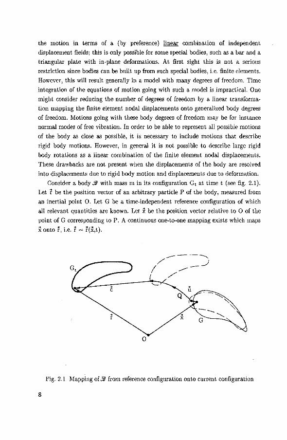
Consider a body 9J with mass min its configuration Gt at time t (see fig. 2.1).
Let t be the position vector of an arbitrary partieleP of the body, measured from
an inertial point 0. Let G be a time-independent reference configuration of which
all relevant quantities are known. Let x be the position vector relative to 0 of the
point of G corresponding to P. A continuous one-to-one mapping exists which maps .. .. . .. .. (.. ) x onto r, I.e. r "" r x,t .
Fig. 2.1 Mapping of 9J from reference configuration onto current configuration
8
The body in Gt can be considered as the result of a deformation of the body in
G with displacement field u(x,t), foliowed by in Succession a rigid body rotation
about 0 defined by the proper orthogonal tensor Q(t), and a rigid body translation
defined by the vector ê(t)
r(x,t) = ê(t) + Q(t)·{x + u(x,t)}. (2.1)
The vector df between t.wo neigbbouring points in Gt and the vector dx between
the corresponding points in Gare related by
ctr = Q(t)·{dx + u(x+dx,t) ii(x,t)}. (2.2)
This equation can be rewritten as
(2.3)
where, for infinitesimally smal! dx, F is the deforrnation tensor by
(2.4)
Here, V is the gradient operator referred to G.
The acceleration and a virtual displacement of a partiele are obtained by
differentiating (1) twice with respect to time and by taking the variation of (1),
respectively. This yields
•• •• + • ..
.. .. Q {.. [.. (.. ..)] .. (.. .. ) .. .. .. } r = c + · w x w x x + u + w x x + u + 2w x u + u , (2.5)
or = bê + Q·{O?t x c:x + ii) + óil}, (2.6)
where w and 67r are the axial veetors of the skew-symmetric tensors Qc · Q and
Qc · óQ, respectively.
The angular velocity vector w differs from the usual angular velocity vector,
which is defined as the axial vector of Q· Qc. The reason for introducing this
alternative angular velocity vector is that then the rotation tensor Q can be
factored out in (5) which is advantageous in the derivation of the equations of
rnotion. The same applies for the virtual rotation vector Mr.
The displacement field of the body bas been resolved into a displacement field
due to deformation defined by ii and a displacement field due to a rigid body
motion defined by c and Q. In order to get a unique resolution, the displacement
field due to deformation is not allowed to represent a rigid body motion. Two kinds
9

of conditions for preventing rigid body motioru; can bo found in literature, namely,
condîtions for displacements of selected particles of tbe body and conditions lor
mean displac\lffients of the body (Koppens et aL, 1988). The first kind of conditions
is used by, among others, Sunada and Duhowsky (1981), Singh et al. (1985),
Agrawal and Shabana (1985), and Haug et al. (1986). The secoud kind of conditions
is used by Agrawal and Shabana (1985), McDonough (1976), and others.
Conditions for displacem.ents of selected particles. This kind of conditions is also
used in finito element analyses of structures (Przemieniecki, 1968). It cornes to
prescrihing displacements due t.o deformation of a numher of selected particles to
prevent rigid body motion. For example, the displacements due to deformation of
one partiele ~ are required to be zero:
(2. 7)
Now, the body can still perfarm rigid body rotations around Pc- Hence, in addition,
rigid body rotations have to be prevented. Thïs may be achieved by constraining
the rotatien of a hody-fixed frame (cf. Singh et al., 1985), or by prescrihing
displacement components of other partïcles. In the latter case rigid body motions
can be preven ted hy prescrihing altogelher six suitably chosen displacement
components. When additional displacement components are prescribed, only a
restricted class of all possible displacement fJelds cao he descri bed.
Conditions for m.ean dispiacemenis ojthe body. A rigid body translation involves
a displacement of the centre of mass. Consequently, a displar.ement field ii cannot
represent a rigid body translation when ït does not cause a displacement of the
centre of mass. This cao he expresscd mathematicaJly as
f p ii cLQ = 0, g
(2.8)
where p is the mass deusîty of G and n is the refercnce volume. Thc translation
vector è wiJl represent the traru;lation of the centre of mass of the body when this
condition is used,
The displacement field due to an infinïtesimally smal! rigid body ·rotation
around 0 can.be represented by the vector field
(2.9)
wherc x is the rotatien angle and eis a unit vector paraHel to the rotation a.xis. Jt can ho seen that the displacements due to this rigid body rotation are perpendicular
to x. Consequently, a displacement field n cannot repcesent a rigid body rotation
10
whcn it is on R mean parallel to x. This can be expressed mathematica.lly as
r . . . ).,PX <u dfl = 0. !l
(2.10)
(p bas been used as a weighting factor in order to cancel some terms in t.he
equations of motion.) Examples of displacement fields satisfying (8) and (10) are
modes of free vibrat.ion (Ashley, 1967).
When in addition to condition (8), the centre of mass in the relerenee
conflguration is ebasen to coincide with 0, some more terros in the equations of
motion will cancel.
2.3 The eouations of motion of a deformable body
The equations repreaenting local balance of linear momenturn at an interior point of
the body referring to the relerenee configuration are given by (cf. Malvern, 1969)
(2.11)
• where T is the second Piola-Kirchhoff stress tensor and b is a specific body laad
vector. lt is preferabie starting from the equations of motion in this farm tostarting
from the more well-known Cauchy's equations of rnotion, because the latter would
require a transformation of variables referrîng to the current configuration onto
variables referring to the reference configuration. This transformation has a.lready
been carried out for the equations of motion inthefarm (ll). The body is assumed to be stress-free in tbe reierenee configuration. Then, lor
isotropie linear elastic material b€haviour, T is related to the strain by (cl. Gurtill,
1981)
T = 2 IJ E + À tr(E) I, (2.12)
where f1 and A are the Lamé elastic consta.nts, I is the identity tensor, and Eis the
Green-Lagrangestrain tensor, defined by
E t{Fc·F I}. (2.13)
Camparing this expressimt with the expression lor the deformation tensor ( 4)
reveals that thc Green-Lagrange strain tensor does not depend on the rigid body
motion. (13) may be linearized in case the gradients of the displacements due to
deformation are smal!. In genera!, this would nat be allowable in case the
displaoements had not been resolved into displacements due to a rîgid body motion
11
and displacements due to deformation.
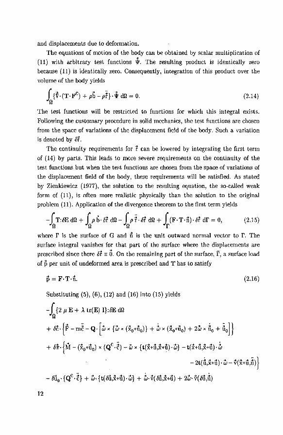
The equations of motion of the body can be obtained by scalar multiplication of
(11) with arbitrary test functions iP. The resulting product is identically zero
because (11) is identically zero. Consequently, integration of this product over the
volume of the body yields
L {v. CT. r) + pb -Ph. iP <ID = o. u
(2.14)
The test functions will be restricted to functions for which this integral exists.
Following the customary procedure in solid mechanics, the test functions are chosen
from the space of variations of the displacement field of the body. Such a variation
is denoted by tft. The continuity requirements for r can be lowered by integrating the first term
of (14) by parts. This leads to more severe requirements on the continuity of the
test functions but when the test functions are chosen from the space of variations of
the displacement field of the body, these requirements will be satisfied. As stated
by Zienkiewicz (1977), the solution to the resulting equation, the so-called weak
form of (ll), is often more realistic physically than the solution to the original
problem (11 ). Application of the divergence theorem to the first term yields
-lT:óEd!l+ fph·lffdn- ip;·fl<ID+ .f.<F·T·n)·lftdr o, (2.15) u u u r
where r is the surface of G and i:i is the unit outward normal vector to r. The
surface integral varrishes for that part of the surface where the displacements are
prescribed sirree there tft 0. On the remairring part of the surface, I', a surface load
of p per unit of undeformed area is prescribed and T has to satisfy
12
Substituting (5), (6), (12) and (16) into (15) yields
-i {2 p, E + À tr(E) I}:óE d!l u
+ 6ê· {F-m~ Q· [ w x {w x (Xo+Û0)} + i1 x (x0+Û0) + 2w x iÏ0 + iio]} ct { .. (.. .. ) (Qc :;) .. { (.. .. .. ..) .. } (.. .. .. ..) -> + o11'· M- x0+u0 x ·c - w x t x+u,x+u ·w - t x+u,x+u ·w
(2.16)
- 2t(ïi.X+û). w- v(X+û,ä)}
- óû0• { Qc. ~} + w· { t( óii,x+u). w} + iir. v( óii,x+ii) + 2w· v{ óii,il)

where
F ipb dQ +Lp df, n r
M: = JP {(x+ii) x (Qc·b)} dn + L{(x+ii) x (Qc·p)} dî:', n r
x0 =lp x dil, n
u0 = Jpu dn, n
t(a,b) iP {(a· b)I- ah} dil n
...... Jp(axb)dil v(a,b) n
.... V a,b,
.. .. V a,b.
(2.17)
(2.18)
(2.19)
(2.20)
(2.21)
(2.22)
(2.23)
The first term of (17) represents the variation of the strain energy 8U of the body
due to a virtual displacement óf. In general, this expression is too complicated to
evaluate; consequently approximations are used instead. For example the
expression for the Green-Lagrange strain tensor (13) is aften linearized. Also the
body may be approximated by a two- ( one-) dimensional body in case one ( two)
dimension(s) of the body is (are) considerably smaller compared with the other two
(one) dimensions using an assumption from which the displacementsof an arbitrary
material point of the body can be written in terms of the displacement of a plane
(line). With such a two- (one-) dimensional body goes an approximate expression
for its strain energy. An example of such a body is a plate (beam).
As has been mentioned already at the end of section 2.2, some terms will cancel
in the equations of motion when the mean displacement conditions (8) and (10) are
used for eliminating rigid body motions. Substitution of successively (8) into (21 ),
and (10) into (23) yields
.. .. u0 = 0. (2.24)
v(x,ii) o. (2.25)
Consequently, also the time derivatives and variations of u0 and v(x,ü) vanish.
13

When the centre of mass of the reference confuguration is chosen to coincide with
0, also
~0 = 0.
Substitution of (24)-(26) into (17) yields
-i {2 p, E + ,\ tr(E) I}:óE dQ Q
+ óê·{F m~}
d {M.. .. { c· ...... ) .. 1 ( ........ ) -+ c-+ .... ) .. ..c .. :;)} + 01r· - w x t x+u,x+u · w - t x+u,x+u · w- 2t u,x+u · w- v u, u
. . + w·{t(bÛ,~+u)·w} + w·v(bÛ,û) + 2w·v(bÛ,û)
(2.26)
(2.27)
From a comparison of the coefficients of óê in (17) and (27), it is observed that in
(27) the rotation and the displacement due to deformation are not coupled with the
translational motion. Oomparing the coefficients of tnr reveals that the coupling
between the rotational and the translational motion has vanished and that the
coupling between the rotational motion and the displacement due to deformation is
reduced. To conclude, also coupling due to terms that involve bÛ is reduced. All
this may be advantageous in the numerical evaluation of the equations of motion
since firstly, less terms have to be evaluated and secondly, the mass matrix has
become more sparse. This is investigated more closely insection 5.2.
2.4 Apnroximate equations of motion: Galerkin's method
The weak form of the equations of motion of a single body have been presented as
equations (17) in the preceding section. The contribution of the displacement due to
deformation û makes that in general a closed-form solution to this equation does
not exist or is not feasible. That is why one resorts to an approximate solution for
ii. This solution is sought in a certain N-dimensional vector space of vector-valued
functions defined on Q. Then it can be represented as a linear combination of N
functions that constitute a base of this vector space. In general (17) will not be
satisfied by this approximate solution for any variation. In solid mechanica one
usually only requires that (17) is satisfied for variations that can be written as a
14

linear combination of the N base functions. From this condition the N unknown
coefficients in the approximate solution can be determined. This procedure is
known as Galerkin's metbod (Zienkiewicz, 1977). It leads to a system of ordinary
differential equations which can be solved with numerical integration routines.
The above-mentioned vector space must be chosen such that its elements satisfy
the same kinematic conditions as û. Further, its elements must be continuons and
once piecewise continuous1y differentiable such that (17) can be evaluated. In case
the body has been approximated by a one- or two-dimensional body, the
accompanying approximate expression for the strain energy may contain secoud
order derivatives of the displacement field u. Then the elements of the vector space
and their first derivatives must be continuous, and their second derivatives must be
piecewise continuous.
Let *(x) be a column matrix of N vector-valued functions ~i(x), i = 1, 2, .... , N,
that constitute a base of the N-dimensional vector space of vector-valued functions.
Then, following Galerkin's method, both û and bû are approximated by a linear
combination of these base functions:
N -+,.. ~ ... -+ T -+ ... u(x,t) Rl k ai(t) <I>i(x) = g (t) p(x), (2.28)
i 1
N
tû(x) Rl L 5aj ~Jiê) 8gT *(x), (2.29) i 1
where g(t) is a column matrix of generalized displacements ai(t), i = 1, 2, ... , ~,
and bg is a column matrix of the arbitrary constants 8ai(t), i 1, 2, ... , N. Bubsti
tution of these equations into (17) yields the variational form of the equations of
motion for the approximated displacement fields (28) and (29):
+81i-·{M-D1 x(Qc·ê) iilx(J·w)-J·~-2{(_ll)2)·w gl:Q3}
+bgT{r-~·(Q·Ç2)+w·(I)2·w) ~·:03+2w·(Q7Q)-.Qsg-} ro, (2.3o)
where
(2.31)
15
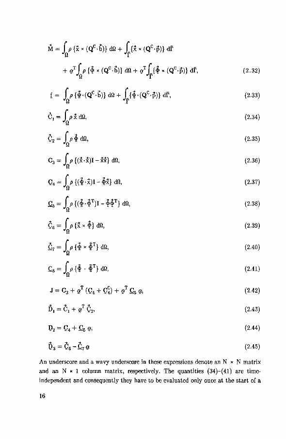
M =lP {x x (Qc·b)} dO+ L{x x (Qc·p)} <lf o r
+ rl ip {~x (Qc·b)} dO+ rl L{~ x (Qc·p)} dÏ\ o r
ê1 = ipx do, ll
C2 ip~ dO, 0
c3 = iP {(x·x)I- xx} do, (}
C4 lPH~·x)I-~it}<ID, o
~ = ip{(~·~T)l-~~T} d!1, o
i .... T .CS = p { ~ • ~ } dO, ll
(2.32)
(2.33)
(2.34)
(2.35)
(2.36)
(2.37)
(2.38)
(2.39)
(2.40)
(2.41)
(2.42)
(2.43)
(2.44)
(2.45)
An underscore and a wavy underscore in these expressions denote an N x N matrix
and an N x 1 column matrix, respectively. The quantities (34)-(41) are time
independent and consequently they have to be evaluated only once at the start of a
16

numerical simulation. They can be determined once the base functions ~(x) have
been chosen.
2.5 Approximate eguations of motion in component form
The equations of motion as presented in the preceding section are in symbolic
vector/tensor form. For computational purposes these equations must be rewritten
in terms of the components of the veetors and tensors relative to some base. All
veetors and tensors can easily be written in terms of their components relative to an
inertial base thanks to the fact that the reference configuration is inertial.
Consequently, there is noneed to specify the base relative to which a certain vector
or tensor is written. This is in contrast to the usual description found in the
literature where both an inertial base and a body-fixed base is are introduced
(Casey, 1983; Sol, 1983; Mclnnis and Liu, 1986).
Let the veetors and tensors be written in terms of their components relative to a
right-handed orthorrormal inertial base Ç. The components of veetors and tensors
wiJl be stored in, respectively 3 x 1 column matrices and 3 x 3 matrices. Veetors
in cross-product terms are replaced by the matrix representation of the correspond
ing skew-symmetric tensors which will be denoted by a wavy superscript (cf. A.l).
Elements of the matrices defined in the preceding section are indicated by their row
and column indices in order to obtain equations of motion in a forrn suitable for
computer implementation. Using this notation and making use of the fact that -> ->T ( ) 12 • 12 I, the third-order unit matrix, the equations of motion 30 become in
component form
DÇT{f mÇ .Q[.i!:!.i!:! 1)1- .Ü1~ + 2.il:!f á(j)Ç2(j) + f ä(j)Ç2(j)]}
+ 81l { M- .Ül.QT ç .i!:! J. \!)- J.~- 2{y á(j)Ih(j)}w r ä(j)Q3(j)}
+ r 8a(i){f(i) Ç~(i).QTÇ + WT!h(i)W- l)~(i)~ + 2\!)Tf á(j)Ç7(i,j)
-1 öWCs(i,j)} = ru. (2.46)
These equations cannot be integrated because the components of the angular
velocity vector, w, cannot be integrated to obtain angular displacements, sirree they
are non-integrable combinations of the first time derivatives of angular displace
ments. These angular displacements are required for evaluating the rotation matrix
.Q. For this reason, differential equations must be added from which the angular
17

displacements ean be obtained.
V arious kinds of angular displaeements are in use, such as Euler angles, Bryant
angles and Euler parameters (Wittenburg, 1977). The rotation matrix Q written in
terms of Euler angles or Bryant angles contains the sine and eosine of these angles.
Evaluation of these goniometrie functions is laborious. These goniometrie functions
cause also a swell of terms when the first or second time derivative of Q is required.
In addition, these angular displacements may suffer from singularities. Due to these
drawbacks usually Euler parameters are preferable. A disadvantage of Euler
parameters is that they are dependent.
The required differential equations for Euler parameters, which have been
derived in appendix B, are
. .l.QT g = 2- !é), (2.47)
where
(2.48)
is a column matrix with Euler parameters, and
n [ -ql qo q3 -q2] ~ -q2 -q3 Qo ql ·
-Qs q2 -ql qo
(2.49)
In literature, w and (gare often written in terms of the angular displacements
and their first and second time derivatives. This leads to more extended equations
of motion. Moreover, when Euler parameters are used as angular displacements, an
extra equation of motion is obtained. From this and in view of the results described
by Nikravesh et aL (1985) for rigid bodies, it is discouraged to write the equations
of motion in terms of the angular displacements and their first and second time
derivatives.
However, the equations of motion on which the computer program DADS is
based are written in terms of Euler parameters and their first and second time
derivatives. Adapting the program to the above given preferenee would involve
rewriting the program entirely. Because of the lack of the required souree code and
because of the large amount of work involved, the equations of motion are written
partially in terms of Euler parameters, such that only a small part of the program
has to be rewritten. From this the extra equation of motion that has been
mentioned above is introduced. This makes the program less efficient. Consequently
18
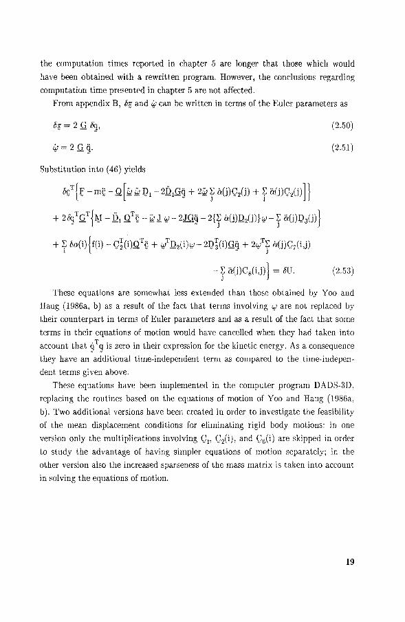
the computation times reported in chapter 5 are longer that those which would
have been obtained with a rewritten program. However, the conclusions regarding
computation time presented in chapter 5 are not affected.
From appendix B, Ins and \61 can be written in termsof the Euler parameters as
\61 2Qg.
Substitution into ( 46) yields
liç} { t"- mÇ- Q [ ~ ~ l)l 2.Ü&g + 2~ f ó:(j)Ç2(j) + r ö:(j)Ç2(j)]}
+ 28qTQT{~1- Ï!1 QTÇ Iid J. i#- 2JGq- 2{~ à(j)J22(j)}'I,J- ~ ö:(j)l)3(j)} - - J J
+ ~ Óa(i){f(i)- Ç~(i)QT I:;+ \6lJ..h(i)'I,J- 2l)~(i)Qq + 2'1,JT~ à(j)Ç7(i,j) 1 - J
(2.50)
(2.51)
-y ö:(j)C8(i,j)} = bU. (2.53)
These equations are somewhat less extended than those obtained by Yoo and
Hang (1986a, b) as aresult of the fact that terms involving '#are not replaced by
their counterpart in terms of Euler parameters and as aresult of the fact that some
terms in their equations of motion would have cancelled when they had taken into
account that <jTg is zerointheir expression for the kinetic energy. As a consequence
they have an additional time-independent term as compared to the time-indepen
dent terms given above.
These equations have been implemented in the computer program DADS-3D,
replacing the routines based on the equations of motion of Yoo and Haug (1986a,
b). Two additional versions have been created in order to investigate the feasibility
of the mean displacement conditions for eliminating rigid body motions: in one
version only the multiplications involving Ç1, Ç2(i), and Ç6(i) are skipped in order
to study the advantage of having simpler equations of motion separately; in the
other version also the increased sparseness of the mass matrix is taken into account
in solving the equations of motion.
19
chapter 3
Generating base functions
3.1 Introduetion
In the preceding chapter the displacement field of a body has been resolved into a
displacement field due to a rigid body motion and a displacement field û due to
deformation. The instantaneous displacement field u is an element of a vector space
of vector-valued functions defined on Q which represent displacement fields that do
not contain a rigid body motion. In section 2.4 this vector space has been replaced
by an N -dimensional vector space. Any element of this vector space can be written
in the form of a linear combination of base functions of this vector space. In case
this vector space has been chosen properly the linear ·Combination will be a good
approximation of the actual solution.
In this chapter three methods for generating base functions will be discussed,
namely the assumed-modes method, the finite element metbod and the modal
synthesis method. From examples it will be illustrated how the time-independent
inertia coefficients (2.34)-(2.41) and the stiffness terms originating from the
variation of the strain energy can be derived for these base functions.
3.2 The assumed-modes metbod
In the assumed-modes method analytic base functions are used that are defined on
the entire volume of the body. These can only be generated for regularly shaped
bodies: these are bodies with a geometry that can be described analytically.
Consequently, the assumed-modes metbod is restricted to such regularly shaped
bodies. Advantage can he taken of knowledge of the behaviour of û by chosing a
vector space that resembles the actual solution well. Then a good approximation
can be obtained with only a few base functions. A more accurate solution will he
obtained when the number of base functions is increased. However this is at the
expense of an increase of the required computation time. Depending on the nature
of the base functions, and the mass and stiffness distributions, the time-independent
inertia and stiffness termscan be evaluated analytically or they must be determined
numerically.
20
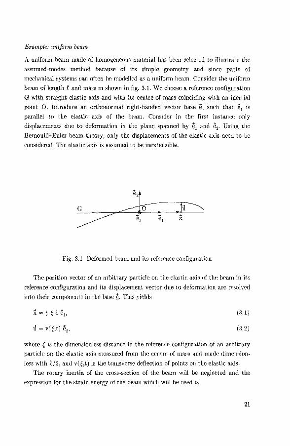
Example: uniform beam
A uniform beam made of homogeneaus material has been selected to illustrate the
assumed-modes method because of its simple geometry and sirree parts of
mechanica! systems can often he modelled as a uniform beam. Consider the uniform
beam of length tand mass m shown in fig. 3.1. We choose a reference configuration
G with straight elastic axis and with its centre of mass coinciding with an inertial
point 0. Introduce an orthorrormal right-handed vector base ~, such that i\ is
parallel to the elastic axis of the beam. Consider in the first instanee only
displacements due to deformation in the plane spanned by e1 and e2. Using the
Bernoulli-Euler beam theory, only the displacementsof theelastic axis need to be
considered. The elastic axis is assumed to be inextensible.
Fig. 3.1 Deformed beam and its reference configuration
The position vector of an arbitrary partiele on theelastic axis of the beam in its
reference configuration and its displacement vector due to deformation are resolved
into their components in the base ~- This yields
(3.1)
(3.2)
where Ç is the dimensionless distance in the reference configuration of an arbitrary
partiele on the elastic axis measured from the centre of mass and made dimension
less with t/2, and v( Ç,t) is the transverse deflection of points on theelastic axis.
The rotary inertia of the cross-section of the beam will be neglected and the
expression for the strain energy of the beam which wiJl be used is
21
1
u= (4EI3jt3) j{lPvjaÇZ}2dÇ, (3.3) -1
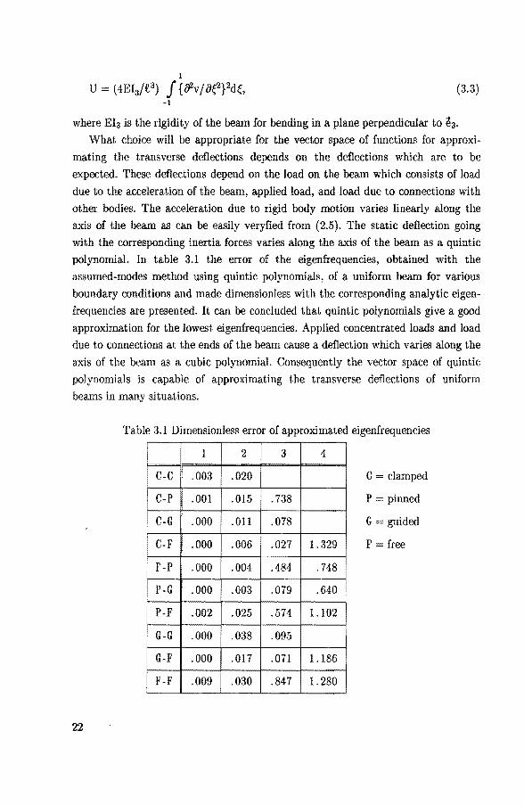
where El3 is the rigidity of the beam for bending in a plane perpendicular to ih. What choice will be appropriate for the vector space of functions for approxi
mating the transverse deflections depends on the deflections which are to be
expected. These deflections depend on the load on the beam which consists of load
due to the acceleration of the beam, applied load, and load due to connections with
other bodies. The acceleration due to rigid body motion varies linearly along the
axis of the beam as can be easily veryfied from (2.5). The static deflection going
with the conesponding inertia forces varies along the axis of the beam as a quintic
polynomial. In table 3.1 the error of the eigenfrequencies, obtained with the
assumed-modes metbod using quintic polynomials, of a uniform beam for various
boundary conditions and made dimensionless with the corresponding analytic eigen
frequencies are presented. It can be concluded that quintic polynomials give a good
approximation for the lowest eigenfrequencies. Applied concentrated loads and load
due to connections at the ends of the beam cause a deflection which varies along the
axis of the beam as a cubic polynomial. Consequently the vector space of quintic
polynomials is capable of approximating the transverse deflections of uniform
beams in many situations.
22
Table 3.1 Dimensionless error of approximated eigenfrequencies
i 1 2
I C-C .003 .020 I C-P .001 .015
C-G .000 .011
I C-F .000 .006
F-P .000 .004
P-G .000 .003
P-F .002 .025
G-G .000 .038
G-F .000 .017
F-F .009 .030
3 4
.738
.078
.027 1.329
.484 .748
.079 .640
.574 1.102
.095
.071 1.186
.847 1.280
I
C = clamped
P = pinned
G guided
F free

Consicter the arbitrary quintic polynomial
(3.4)
Deflections approximated with such a polynomial include also rigid body motions,
which are not allowed in the displacement field û as has been discussed in the
preceding chapter. When base functions are selected that do not contain rigid body
motions, also the linear combinations (2.28) and (2.29) will be free of rigid body
motions. For the present example the mean displacement conditions wil! be used to
eliminate rigid body motions since these conditions yield the most simple equations
of motion. Condition (2.8) applied to the quintic polynomial ( 4) leads to
a0 + (1/3)~ + (1/5)a4 = 0. (3.5)
Condition (2.10) leads to
(1/3)a1 + (1 /5)a3 + (1/ï)a5 = 0. (3.6)
Displacement fields of quintic polynomials (4) that satisfy (5) and (6) are free of
rigid body motions.
A base of the space of quintic polynomials that satisfies these conditions can be
chosen in many ways. In order to minimize the number of nonzero terms in the
mass matrix the base functions will be chosen orthogonal. Consequently, the
off-diagonal termsof the rnadal mass matrix (2.41) will vanish. Base functions will
be chosen to be either odd or even in order to be able to take advantage of possible
symmetry and in order to make subsequent derivations easier. The base that has
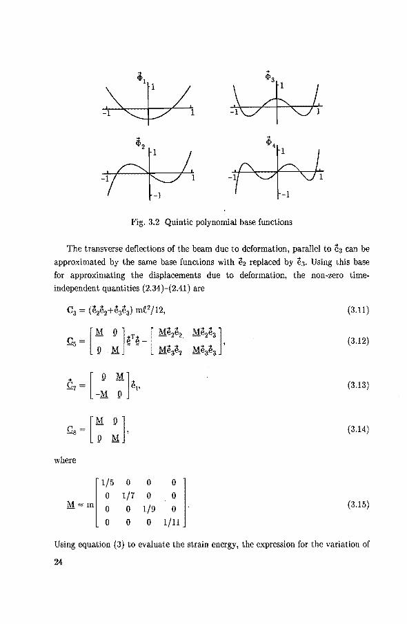
beenchosenon account of these conditions is
(3. 7)
(3.8)
(3.9)
(3.10)
These polynomials are normalized such that they equal 1 for Ç 1. These functions
are plotted in fig. 3.2.
23
~~L -1 1
Fig. 3.2 Quintic polynomial base functions
The transverse deflections of the beam due to deformation, parallel to ês can he
approximated by the same base functions with ih replaced by és. Using this base
for approximating the displacements due to deformation, the non-zero time
independent quantities (2.34)-(2.41) are
Cs (.... .. .. ) t2/ e2e2+e3e3 m 12, (3.11)
~ [; :J~T~ [ Mê2ê2 Mê2ê3 ]
Mê3ê2 .. .. ,
Me3e3
(3.12)
.. [ 9 M ] .. .Q7 et, -M 9
(3.13)
[; :]. (3.14)
where
1/5 0 0 0
0 1/7 0 0 M=m 0 0 1/9 0 (3.15)
0 0 0 1/11
Using equation (3) to evaluate the strain energy, the expression for the variation of
24
tbe strain energy becomes
OU= ógT [ ~3 Q l g, K2
(3.16)
wbere
144 0 480
0 1 EI. 0 1200 0 3360 =-1
{la 480 0 5520 0 .
0 3360 0 18480
(3.17)
3.3 Tbe finite element metbod
Tbe finite element metbod is extensively used for tbe determination of tbe dynamic
behaviour of structures. Basically, the finite element metbod as described in this
section for approximating the displacement field due to deformation is tbe same as
the regular finite element metbod. However, because of the subdivision of
displacements, extra inertia properties of the fini te elements are required (Shabana,
1986). In this section an overview of the general procedure of the finite dement
metbod is given. For a more detailed treatment the reader is referred to the
literature which is plentiful available, e.g. Przemieniecki (1968), Ziekiewicz (1977),
and Rao (1982). The derivation of the element properties is illustrated for a truss
element with linearand quadratic shape functions.
Tbe assumed-modes method as presented in the preceding section is inadequate
for most practical problems since most bodies encm1ntered in practice are not
regularly shaped. The finite element methad provides a way of generating base
functions for arbitrarily shaped bodies. The basic idea is to subdivide bodies into
small polyhedral parts called finite elements. For such elements it is possible to
generate base functions. In general it is not possible to built up the volume of a
body exactly with such elements due to the sha.pe of the body. This error will
deercase when the number of elementsis increased.
On each finite element a number of points is selected, the nodes, usually
situated on the boundary of the element. Nodes on the common boundary of
neighbouring elements must coincide. In order to achieve this, the nodes on the
boundaries are chosen in a systematic way, for instanee at vertices. In order to
satisfy the continuity requirements in a systematic way the base functions are
chosen such that they are equal to unity at one node and zero at all the other
25
nodes; they are only nonzero for the elements to which the node belongs except for
the boundaries that do not contain the node. Since base functions extend only over
elements with common nodes, base functions defined on elements that have no
common nodes are orthogonal which renders the inertia and stiffness matrices of the
finite element model of the body sparse. Because base functions are such that they
are equal to unity at just one node and zero at all the other nodes, the coefficients
of the base functions in the approximation for the displacement field ii (2.28)
repreaent noclal displacements. Consequently, the componentsof the nodal displace
ments relative to a common base can be used as the unknown coefficients in the
linear combination (2.28). The functions defined on an element are called the
element shape functions. A base function corresponding to a node is the junction of
the element shape functions which equal unity at that node.
In general, a more accurate solution will be obtained when the number of finite
elements is increased. In order to ensure convergence, the shape functions must be
such that displacement fields can be described that correspond to a rigid body
motion of the element, and displacement fields that correspond to a constant strain
condition (Zienkiewicz, 1977), next to the continuity requirements. One often
prefers to use polynomials as shape functions because inertia and stiffness properties
can then be evaluated in closed form. The required minimum degree of these
polynomials is determined by the convergence requirements on the shape functions.
In general, for a given desired accuracy of the solution the total number of
unknowns in a problem can be reduced when the degree of the polynomial is
increased especially when the gradient of the displacement field varies sharply.
However this leads to less sparse matrices and the effort required for formulating
and evaluating the element inertia and stiffness properties increases. Consequently
numerical experiments are necessary todetermine whether it is advantageous to use
polynomials with a higher degree than required. The number of nodes and the
degree of the polynomial are linked in such a way that the total number of noclal
displacements équals the number of coefficients in the polynomial.
The exact expression for the variation of the strain energy as gîven by the first
term of (2.17) and its linearized counterpart contain only first order spatial
derivatives of the displacement field due to deformation. Consequently the base
functions must be continuons and piecewise continuously differentiable. Linear
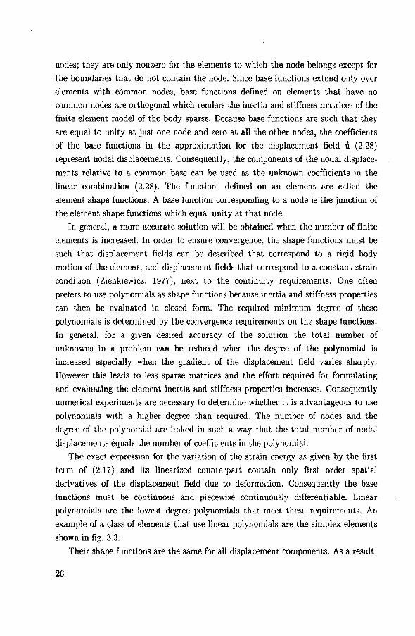
polynomials are the lowest degree polynomials that meet these requirements. An
example of a class of elements that use linear polynomials are the simplex elements
shown in fig. 3.3.
Their shape functions are the same for all displacement components. As a result
26

Fig. 3.3 Simplex elements
the displacement field within the element can be easily written in terms of the
nodal displacement components relative to a base common for all elements. The
shape functions can be used for interpolating the position vector of an arbitrary
partiele of the element from the position veetors of the nodes of the element in the
reference configuration. When both the displacement field and the position vector
are written in terms of their components relative to a common base then there will
be no need to transferm the element properties to a conunon base. This applies to
all elements with shape functions that are independent of the orientation of the
element.
Sirree the shape functions of these elements can describe large rigid body
motions of the element, they can be used to describe the displacement field of a
body without resolving the displacements into rusplacements due to a rigid body
motion and displacements due to deformation. In fact this is dorre in literature for
analyzing mechanica! systems, e.g. the truss element considered by Jonker (1988).
However, many regular finite elements are not capable of descrihing large rigid
body rotations. Consequently special elements must be derived in case the displace
ment field of a body is not resolved into displacements due to a rigid body motion
and displacements due to deformation. Jonker (1988) presented a spatial beam
element for this purpose. The advantage of such an element description is that the
contribution of the inertia of a body is taken into account by the assembied mass
matrix, and the equations of motion of a system of boclies are ordinary differential
equations which can be obtained by the regular assembly process. However, this has
the two already mentioned drawbacks: firstly, nonlinear strain-displacement
relations have to be used even when the strains are smal! and secondly, it is not
possible to reduce the number of degrees of freedom using the rnodal synthesis
method to be described in the next section. This way of description, i.e. without
resolving the displacement field of the body, is not further considered in this thesis.
One may prefer to use different shape functions because the behaviour of one
27

displacement component is different from the behaviour of other components. This
occurs especially with one- or two-dimensional elements in a space of higher
dimension. Particularly the behaviour of tangential displacements and transverse
displacements generally differ: a transverse displacement field that causes bending
must satisfy more severe continuity requirements because the expression for the
variation of the strain energy due to bending contains secoud order derivatives,
whereas its counterpart for tangential displacements contains first order
derivatives; in case no bending is allowed the displacement field must be such that
the element remains straight, i.e. the transverse displacement must vary linearly
whereas the tangential displacement may be described by a higher degree
polynomial. The shape functions are such that only infinitesimally small rigid
rotations of the element can be described. When different shape functions are used
it is necessary to transform quantities from an element base to a base common to
all elements.
For all finite elements inertia properties have to be evaluated such that the
time-independent inertia coefficients (2.34)-(2.41) can be determined. Only .Q8 is
required for regular finite elements; the other coefficients are required as a result of
the resolution of displacements into displacements due to rigid body motion and
displacements due to deformation. The inertia and stiffness properties of an entire
body can be obtained by adding the contribution of all elements. This process is
identical to the assembly process of the standard finite element method. Rigid body
motions of the assembied finite element model can be prevented in the same way as
is customary for the standard fini te element method.
The derivation of the element inertia and stiffness properties will be illustrated
with two examples each from one of the two categodes of elements discussed above,
namely a uniform pin-jointed truss element with respectively a linearly and a
quadratically varying displacement field.
Example 1: linear pin-jointed truss element
Consider the uniform pin-jointed truss element of length .t and mass m shown in
fig. 3.4. For a truss element at least two nodes have to be introduced in order to be
able to describe displacement fields that correspond to a rigid body motion of the
element and displacement fields that correspond to a constant strain condition:
with two nodes correspond six unknown displacements; five are required to describe
a rigid body motion (a truss element has only five rigid degrees of freedom since a
rotation about its axis is immaterial), consequently one degree of freedom is left for
descrihing a constant strain condition. Introduce two nodes situated at the
28

Fig. 3.4 Linear truss element
endpoints of the element. The constant strain condition corresponds to a linearly
varying displacement along the axis of the element. From this the displacement of a
partiele P of the element can be written in terms of its nodal displacements
(3.18)
where Ç is the distance between P and node 0 in the undeformed configuration and
made dimensionless with t. This equation can be rewritten in a form equivalent to
(2.28)
T [(1-Ç)ll.. T .. u(Ç,t) = [ y~(t) y 1(t)] Ç I ç eQ' (t) eil?(Ç), (3.19)
where y0 and y1 are the matrix representation of u0 and u1 relative to an inertial
base ~; the subscript e refers to the contribution of the element to the quantity
concerned. The shape functions of this element are (1-Ç) ~ and Ç Ç. The position vector of an arbitrary partiele in the reference configuration can be
expressed in terms of the position veetors of the nodes in the referenee configuration
.. T T [(1-Ç)Il.. T .. x(Ç) = [ ~o ~h] Ç I Ç = e~ eil?(Ç), (3.20)
where ~0 and ~1 are the matrix representation of the position veetors of the nodes in
the referenee configuration. From this description of the displacement field of the
truss element, its inertia and stiffness properties can be evaluated. Substitution of
(19) and (20) into the time-independent inertia coefficients (2.34)-(2.41) yields
(3.21)
29

(3.22)
(3.23)
(3.24)
(3.25)
(3.26)
(3.27)
m [ 2I I] eik= 6 ' I 2I (3.28)
The matrix & is the regular mass matrix of a truss element (Przemieniecki, 1968).
The linearized expression for the strain energy of a truss element is 1
U = ~~ J { B(ii · l)/ oe}2dÇ = e!l eK eQ', (3.29) 0
where EA is the extensional rigidity of the truss element and l is a unit vector
parallel to the element in the reference configuration
(3.30)
and
(3.31)
with
(3.32)
30

e.K. is the regular stiffness matrix of a bar element (Przemieniecki, 1968).
Example 2: quadratic pin-jointed truss element
When a truss element is loaded by a distributed axial load or when it is not
uniform, it may be advantageous to approximate the displacement field with a
quadratic or higher degree polynomial. Consider the case with a quadratically
varying displacement field. In order to remain straight, the transverse displacement
field must vary linearly along the axis of the element. Consequently, the axial and
transverse displacement fields must be interpolated differently. The displacement of
a partieleP on the element can be written in the form (see fig. 3.5)
û(Ç,t) = (1-Ç) û0(t) + Ç i11(t) + 7(t) 4Ç(l-Ç)t*, (3.33)
where 1 is a generalized displacement and e* is a unit vector which is parallel to the
element in its deformed configuration. The polynomial in the last term has been
chosen such that it equals zero in the endpoints of the element. An extra node with
unknown axial displacement must be introduced in order to be able to rewrite this
expression in terrus of unknown nodal displacements. However, the element
properties will become more involved when they are referred to unknown nodal
displacements as compared to the unknowns introduced in (33). Therefore the
element properties will be derived using (33).
Equation (33) is not of the form (2.28) because e* depends on iio and Û1. When
the rotation of the element caused by deformation is smal!, t* equals approximately
f., i.e. the unit vector which is parallel to the element in its undeformed
configuration. Therefore {*is replaced by f. Using this approximation, (33) can be
written in the form
Fig. 3.5 Quadratic truss element
31

[
{1-Ç)l
û = [ y~ 'Y vi J 4Ç{1-Ç)fr ~.
ç I (3.34)
where f is a column matrix with the components of Ê relative to ~. This coefficient
is the result of the transformation from an element base to a common base ~.
The position vector of an arbitrary material point can be expressed in terrus of
the position veetors of the end nodes using (20).
The inertia and stiffness properties of the quadratic truss element can be
evaluated from this description of the displacement field. Substitution of (20) and
(34) into the time-independent inertia coefficients (2.34)-(2.41) yields
r[I] .. !me~ I ~' (3.35)
m T ..
[ 31 l
0 :~ ~. (3.36)
(3.37)
(3.38)
rl lOt; 51 [ wee' lO .... T
5 .. , ]] ~~ f
lOt;::~T .!), = :ffi- 1:~' 16 lOt;T f~ + 10{T~~T 16~T.Ó.~ (3.39)
lOt; lOl 5~f lO .... r 10~~T ~~ f
-[ 2. 2,;l]~. .. m T:; (3.40) eÇ6 -0 2t;~~
2~
32

-l!Ol 10§~
'"1 m T:; 0
T:; 30 10~-~ 10~-~ ,
10ik 10§
(3.41)
10€ 1 16 lO{T .
lOf lOl
(3.42)
The linearized expression for the strain energy of this quadratic truss element is
u ~~ f {a(u· r)/8Ç} 2d{ = H y~ I Yi' J eK [~i ' 0 T
Yt
(3.43)
where the element stiffness matrix eK is given by
(3.44)
A is defined by (32).
The element properties referred to nodal displacements can be calculated from
these element properties. However, this is not necessary when the extra node is not
coupled to other elements. In general, elements will not be coupled via the extra
node sirree that causes a jump in the gradient of the displacement field which
cannot be described by (34). In order to show what transformation is required for
replacing the generalized displacement 1 by nodal displacements, "f must be written
in terms of nodal displacements. Introduce an extra node at { t. Let the axial
displacement at this node be ü. This displacement must be equal to the axial
displacement obtained from (34) for { t. Hence
(3.45)
Consequently, the column matrix with the generalized displacements and the
column matrix of nodal degrees of freedom are related by
[ T TJ [ T - TJ Yo 'Y Y1 = Yo u llt I, (3.46)
33

where
r
I -h 0 l I= -_oo_T 1 _~I-T ,
-h
(3.47)
In order to transfonn the element properties to their counterpart with respect to .. .. noclal displacements, the column matrices eÇ2, eÇ4 and eÇ6 must be premultiplied
.. with I and the matrices ~' eQ7, e.Qg and eK must be premultiplied with I and
postmultiplied with TT.
3.4 Modal synthesis metbod
For boclies with a complex geometry, the finite element metbod generally leads to
models with many degrees of freedom. This is undesirable from a computation costs
point of view: in determining the transient response of a model many equations of
motion must be integrated, and many degrees of freedom lead to a large variation
of eigenfrequencies which reduces the integration time steps. Consequently, a
reduction of degrees of freedom is desirable. The usual procedure to achieve this,
which is called the modal synthesis method, is to use a set of linear combinations of
the base functions generated with the finite element method. Such linear
combinations of finite element base functions may be regarcled as numerically
generated base functions which are the counterpart of the analytic base functions
considered in section 3.2. This approach combines the efficiency of the
assumed-modes metbod and the versatility of tbe fini te element method . .. Let ai> be an n x 1 column matrix of the assembied finite element shape
functions of a body. Then a reduced set of base functions can be obtained with the
transformation
{3.48)
.. where t is an N x 1 column matrix of base functions and ~ is an n x N matrix of
constants. The columns of ~ contain nodal displacements. In general N will be much
smaller than n. The time-independent coefficients for this new set of base functions
can be obtained from the assembied time-independent coefficients obtained with the .. -+ ~T
finite element method by premultiplying aÇ2, aç4 and aç6 with ~ , and
34

premultiplying a.Q5, a.6ï, a.Qs and aK with and postmultiplying the result with L;. An issue of primary concern of the modal synthesis method is the selection of
the matrix L;. To take full advantage of the modal synthesis metbod one should
select the matrix L; such that only a small number of base functions can describe the
displacement field due to deformation of the body satisfactorily. What choice will
be most appropriate depends on the problem at hand. The most widely used choices
originate from the reduction procedures used in structural dynamics.
The standard procedure to determine an approximate solution of the transient
response of structures under time-dependent loads is to express the displacement of
the structure as a linear combination of a reduced set of modes of free vibration
(Przemieniecki, 1968). The corresponding set of equations of motion are uncoupled
and its solution can be easily obtained. Complex structures are often regarcled as an
assembly of substructures. The defonnation of each substructure is represented by a
linear combination of deformation modes. These modes are chosen such that the
equations of motion of the complete structure can be easily obtained from the
equations of motion of the substructures (component mode synthesis method).
Craig (1981) gives an overview of such modes.
The modes used in structural dynamics have distinct properties which facilitate
solving the equations of rnotion. But these properties are not necessarily relevant in
solving the equations of motion of a mechanica! system. Modes of free vibration do
not uncouple the equations of motion (2.30) because of the coupling of displace
ments due to deformation and displacements due to a rigid body motion. Moreover,
the instantaneous modes of free vibration of a body in a system of bodies depend on
the instantaneous configuration of the system, especially when it has a tree
topology. Consequently there is no motive to prefer modes of free vibration above
other displacement fields. Likewise the properties of the modes used in the
component mode synthesis method are not relevant. For all that, these modes have
been used by several investigators: Agrawal and Shabana (1985), and Singh et al.
(1985) used modes of free vibration; Sunada and Dubowsky (1981, 1983) used
component modes.
Yoo and Haug {1986a, 1986c) recognized that less modes are required when in
the case of the presence of concentrated loads, the static deformation due to such
loads is included. Also for structural dynamic problems a more accurate solution
may be obtained when static deformation modes are included (Kline, 1986). Indeed
those modes should be used which can represent the actual deformation of the body
best. The selection of deformation modes will be discussed in section 5.4 with the
help of some examples.
35

chapter 4
The equations of motion of a system of bodies
4.1 Introduetion
The equations of motion of a single isolated deformable body have been derived in
chapter 2. In the present chapter the equations of motion of a system of intercon
nected bodies will be considered. These can be obtained from the equations of
motion of the single bodies by taking the forces caused by the connections into
account.
Connections can be subdivided into energetic, active and kinernatic connections
(Sol, 1983). The forces caused by energetic and active connections can be obtained
frorn constitutive equations. It will be assumed that forces caused by kinematic
connections do not enter into the constitutive equations such as may be the case for
Coulomb friction forces. The forces caused by energetic and active connections can
be deterrnined at the outset and consequently they can be taken into account by
introducing thern into the load integrals of (2.15).
Kinernatic connections restriet relative rnotions of interconnected bodies.
Consequently displacernents of bodies are dependent. The equations relating
displacernents of kinernatically connected bodies are called constraint equations.
Only constraint equations of the forrn
0(~,t) = 0 (4.1)
will be considered, where 8(~,t) is an algebrak function which is once continuously
differentiable with respect to its argurnents and ~ is a column matrix of all scalar
variables that are introduced to describe the kinernatics of the systern of bodies,
narned the generalized displacernents of the systern of bodies. Kinernatic
connections with constraint equations of this forrn or that can be reduced to this
forrn are called holonornic. If a constraint equation does not contain time explicitly,
it is called scleronornic; otherwise it is called rheonornic. Porces going with
kinernatic connections, constraint forces, cannot be deterrnined at the outset. They
rnay be introduced as additional unknowns. A practical way of doing this is by
rneans of the Lagrange multiplier rnethod (Meirovitch, 1970). Then variations of
the generalized displacements of the systern of bodies rnay be chosen arbitrarily.
They rnay also be chosen such that the eenstraint equations are not violated.
36

Variations of the generalized displacements which are consistent with the constraint
equations are termed virtual displacements. The work done by all constraint forces
due to virtual displacements equals zero (Rosenberg, 1977) and consequently these
forces do not appear in the assembied variational form of the equations of motion.
In section 4.2, energetic and active connections will be considered. The
constraint equations for kinematic connections differ for the relative and the global
description. This will be illustrated in section 4.3. Procedures for obtaining
generalized virtual displacements will be given in section 4.4 for the relative and
the global description. These are used for obtaining the equations of motion of a
system of bodies.
4.2 Energetic and active connections
The forces caused by both energetic and active connections can be obtained from
constitutive equations, which relate the forces, the relative displacements and
veloeities of the interconnected boclies and the time history of these quantities, and
external parameters. The difference between energetic and active connections is
that the former do not increase the total mechanica! energy of the system of bodies,
whereas the latter may increase the total mechanica! energy. Examples of energetic
connections are springs and viscous dampers; an example of an active element is an
actuator. The derivation of the contribution of energetic and active connections to
the equations of motion of a system of boclies is demonstrated with a linear spring,
a linear viscous damper and an actuator.
Consider the bodies ,2i and ,2i interconnected by a linear spring, a linear
viscous damper and an actuator as shown in fig. 4.1. Let the spring, the damper,
Fig. 4.1 Conneetion of spring, damper and actuator
37
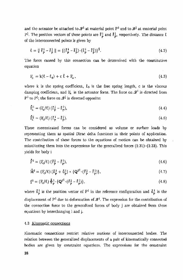
and the actuator be attached to~i at material point pi and to~i at material point
Pi. The position veetors of these points are r; and r~, respectively. The distance t of the interconnected points is given by
(4.2)
The force caused by this conneetion can be deterrnined with the constitutive
equation
(4.3)
where k is the spring coefficient, to is the free spring length, c is the viscous
damping coefficient, and &. is the actuator force. The force on ~i is directed frorn
pi toPi; the force on~i is directed opposite:
pci = (F;;/t) (r~ r;),
FJ = (F;;/t) (r; r~).
(4.4)
(4.5)
These concentrated forces can be considered as volurne or surface loads by
representing thern as spatial Dirac delta functions in their points of application.
The contribution of these forces to the equations of motion can be obtained by
substituting thern into the expressions for the generalized forces (2.31 )-(2.33). This
yields for body i
pi= (F;;/t) (r~- r~),
M:i = (Fc/t) C*·t +u;) x {Qic·(r~- -r;n, fi = (Fcft) i; ·{QiC.(t~ r;)},
(4.6)
(4.7)
(4.8)
where i~ is the position vector of pi in the reference configuration and ii~ is the
displacement of pi due to deforrnation of .ll'i. The expression for the contribution of
the conneetion force to the generalized forces of body j are obtained frorn these
equations by interchanging i and j.
4.3 Kinernatic connections
Kinernatic connections restriet relative rnotions of interconnected bodies. The
relation between the generalized displacernents of a pair of kinernatically connected
boclies are given by constraint equations. The expressions for the constraint
38
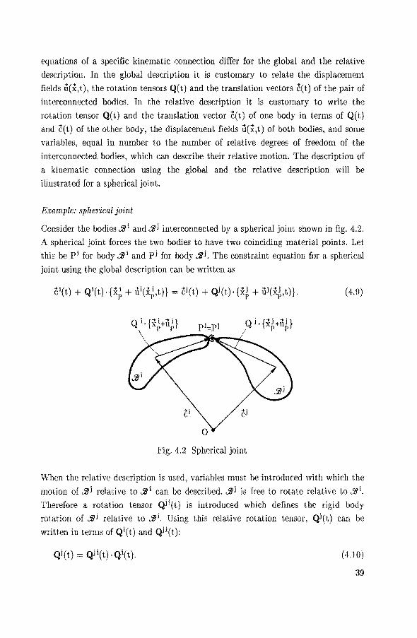
equations of a specific kinematic conneetion differ for the global and the relative
description. In the global description it is customary to relate the displacement
fields u(x,t), the rotation tensors Q(t) and the translation veetors c(t) of the pair of
interconnected bodies. In the relative description it is customary to write the
rotation tensor Q(t) and the translation vector c(t) of one body in terrus of Q(t)
and c(t) of the other body, the displacement fields u(x,t) of both bodies, and some
variables, equal in number to the number of relative degrees of freedom of the
interconnected bodies, which can describe their relative motion. The description of
a kinematic conneetion using the global and the relative description will be
illustrated for a spherical joint.
Example: spherical joint
Consider the bodies $i and $Î interconnected by a spherical joint shown in fig. 4.2.
A spherical joint forces the two boclies to have two coinciding material points. Let
this be pi for body$; and pi for body $Î. The constraint equation fora spherîcal
joint using the global description can be written as
(4.9)
Fig. 4.2 Spherical joint
When the relative description is used, variables must be introduced with which the
motion of $Î relative to $i can be described. $Î is free to rotate relative to $;.
Therefore a rotation tensor Qii(t) is introduced which defines the rigid body
rotation of $i relative to $i. Using this relative rotation tensor, Qi(t) can be
written in termsof Qi(t) and Qii(t):
( 4.] 0)
39
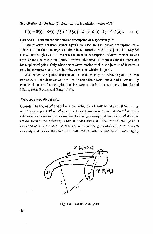
Substitution of (10) into (9) yields for the translation vector of .î/j
(10) and (11) constitute the relative description of a spherical joint.
The relative rotation tensor qii(t) as used in the above description of a
spherical joint does not represent the relative rotation within the joint. The way Sol
(1983) and Singh et al. (1985) nse the relative description, relative motion meaus
relative motion within the joint. However, this leads to more involved expressions
for a spherical joint. Only when the relative motion within the joint is of interest it
may be advantageous to use the relative motion within the joint.
Also when the global description is used, it may be advantageous or even
necessary to introduce variables which deseribe the relative motion of kinematieally
connected bodies. An example of such a conneetion is a translational joint (Li and
Likins, 1987; Hwaug aud Haug, 1987).
Example: translational joint
Consider the bodies $i aud .î/j interconnected by a translational joint shown in fig.
4;.3. Material point pj of $j eau slide along a guideway on $i. When $i is in the
referenee configuration, it is assumed that the guideway is straight aud $i does not
rotate around the guideway when it slides along it. The translational joint is
modelled as a deformable line ( the centreline of the guideway) and a muff which
eau only slide along that line; the muff rotates with the line as if it were rigidly
Fig. 4.3 Translational joint
40
attached to it. Let this line in the reference configuration he parallel to a unit
vector f. The relative motion can he described by one variable, namely the distance
s between the muff and some reference point pi on the line. Due to the translational
joint, a material point of $i must coincide with material point Pj. The position
vector of this material point in the reference configuration is 1t + s€, where 'X~ is
the position veetor of pi in the reference configuration. The eonstraint equation
which describes that these material points must eoineide is
Further, the points of contact cannot rotate relative to one another. It is assumed
that the orientation of the bodies in the reference eonfiguration has been chosen
such that there is no relative rotation within the translational joint. Then the
corrE>,sponding constraint equation is
(4.13)
where Ri(ï1i('X~+s'f,t)) and Ri(u.Ï(x~,t)) account for the rotation due to deformation
at the contact points. This equation ean he rewritten as
( 4.14)
These are nine equations; only three of them are independent due to properties of
rotation tensors. In principle an arbitrary triplet may he ehosen. However, because
generally the rotation tensors due to deformation are linearized the equations on
the diagorral of the matrix representation of this equation cannot be satisfied and
corresponding off-diagonal terms are dependent. When this is taken into account in
seleeting eenstraint equations, the remaining independent constraint equations are
the same as those presented by Hwang and Haug (1987).
In general it is not possible to eliminate the variabie s from these constraint
equations. Consequently, for deriving the constraint equations in the global
description of a translational joint, it is necessary to introduee a variabie whieh
destribes the relative motion.
The eonstraint equations for a translational joint in the relative description are
obtained by solving ci(t) and Qj(t) from (12) and (13). This yields
ci(t) ci(t) + Qi(t). {'X~+ sê + ûi()(~+sÊ,t)}
- Qi(t)·Ri(ïJi(x~+s'f,t))·Ric(ui(xt,t))·{x~ + i1i(x~,t)}, (4.15)
41

( 4.16)
In the relative description, the order of the bodies matters as will become clear in
the next section. When the opposite order of bodies is selected the relative
description of a translational joint becomes
ci(t) = ëj(t) + Qj(t). {x~+ i1j(x~,t)}
-Qj(t)·Rj(û.i(x~,t))·Ric(ûi(x~+sl,t))·{x~ + s~ + ûi(x~+s~,t)}, (4.17)
4.4 The equations of motion of a system of bodies
The equations of motion in component form of a body, which is part of a system of
bodies, can be written symbolically (cf. 2.46)
( 4.19)
where e;ç is a column matrix of the generalized constraint forces that act on the
body. Using the generalized principle of d 'Alembert (Meirovitch, 1970) the
equations of motion for a system of NB bodies become
( 4.20)
The contribution of the constraint forces cancels only when the variations of the
generalized displacements satisfy the variation of the constraint equations with
time held fixed. This variation can be written in the form
H/Jr:= Q, ( 4.21)
where H is the m x n Jacobian matrix of the constraint equations of rank m, and D?;
is an n x 1 column matrix which contains variations of all generalized displacements
of the system of bodies; m is the number of constraint equations and n is the
number of generalized displacements. The rank of the Jacobian will be less than m
42

when the constraint equations are dependent or incompatible. In the former case,
some of the constraint equations can be ignored such that the new Jacobian has full
row rank; the latter case refers to an inconsistent set of constraint equations which
allows no solution. Using (21 ), variations of m generalized displacements can be
written in terms of variations of the remaining n - m generalized displacements.
The latter are independent and may be chosen arbitrarily. The procedure for parti
tioning the virtual displacements into dependent and independent displacements
differs for the global and the relative description. These two approaches will be
considered more closely in the next two sections.
4.4.1 The global description
Wehage and Haug (1982) have presented an automatic procedure for partitioning
displacements into dependent and independent displacements called the generalized
coordinate partitioning method. They decompose the Jacobian .H using full row and
column pivoting into matrices 1, !lu, and 1F such that
J, ( 4.22)
where 1 and !lu are nonsingular lower and upper triangular m x m matrices,
respectively, and the symbol "' denotes that the matrices on either side are equal
apart from a possibly different order of columns due to the decompositioning of .H. The elements of 8?; going with !lu, 8y, can be written in terms of the remaining
elements {jy because !lu is nonsingular:
8y=- (4.23)
Substitution of in Succession n - m linearly independent combinations 8y and the
conesponding variations Ó\J into (20) leads to n - m equations of motion. Usually,
in succession one component of Jy is chosen equal to one and the remaining
components are set equal to zero.
The resulting equations of motion contain still the dependent displacements and
their time derivatives 1j and ij. The dependent displacements can be solved frorn the
constraint equations. Since these are generally nonlinear algebraic equations this
must be done iteratively. 1j and ij can be written in terms of y and y using,
respectively, the first and second time derivative of the constraint equations. Using
these, y can be solved from the equations of motion. Then y eau be integrated using
a standard numerical integration algorithm such as the variabie order explicit
predictor/implicit corrector algorithm DE (Shampine and Gordon, 1975).
43
The efficiency of the procedure outlined above is limited by the requirements for
iterative solution of the dependent generalized displacements from the constraint
equations. This problem may be alleviated by using the relative description.
Another approach is to supplement the equations of motion with the second
time derivative of the constraint equations and to integrate both the independent
and the dependent displacements. This makes solving of the constraint equations
and their first time derivative for the dependent displacements and their first time
derivative superfluous. However, because of numerical errors, the constraint
equations will be violated. Baumgarte (1972, 1978) proposed to replace the secoud
time derivative of the constraint equations by the alternative equation
~(~,t) + 2a$(~,t) + f12<1(~,t) Q, (4.24)
where <1 is a column matrix of the constraint functions, ~ is a column matrix of the
generalized displacements of the system of bodies, and a and /3 are positive
constants. This approach is referred to as the constraint violation stabilization
method. Usually a is chosen equal to /3 which corresponds to a critically damped
system. Due to the extra terms, additional eigenfrequencies are introduced. A
solution to this problem is proposed by Baumgarte (1978). A shortcoming of
Baumgarte's approach is the issue of cboosing proper values of a and /3. Chang and
Nikravesh (1985) proposed a modification of Baumgarte's metbod where the
constauts a and /3 are adjusted each integration time step. However, numerical
errors accumulate due to lack of positive error control of the constraint violation
stabilization method.
Park and Haug (1985, 1986) proposed a bybrid metbod that is the fusion of the
generalized coordinate partitioning metbod and the constraint violation
stabilization method. They partitioned the generalized displacements into
dependent and independent displacements, and integrated both types of
displacements using the extra terms in (24). Error control is imposed only on the
independent displacements. The dependent generalized displacements are corrected
by solving them from tbe constraint equations if the violation of the constraint
equations exceeds a specified error tolerance. Numerical experiments done by Park
and Haug reveal tbat this is required for only a small number of times which makes
their approach more efficient than the generalized coordinate partitioning method.
Their metbod (and the generalized coordinate partitioning method) succeed in
solving problems where the constraint viola.tion method fails due to lack of positive
error control, which makes the hybrid method more stabie than tbe constraint
vialation stabilization method.
44
4.4.2 The relative description
When the relative description is used, the relative motion of a pair of kinematically
connected bodies must be described such that the rigid body motion of one body
can be expressed explicitly in termsof the rigid body motion of the other body, the
displacement fields due to deformation of both bodies, and variables that describe
the motion of the bodies relative to one another (cf. (10)-(11), (15)-(16), and
(17)-(18)). When the system of bodies does not have kinematically closed chains,
the motion of any body of the system can be written explicitly in terms of
independent generalized displacements thns avoiding the need to solve the
constraint equations iteratively.
Consicter a system of bodies without kinematically closed chains. Assume the
system has a tree topology, i.e. one can go from one body toanother along a unigne
alternating sequence of bodîes and kinematic connections. In case such a sequence
does not exist, the system may be thought of to consist of several trees or,
kinematic connections with six degrees of freedom may be introduced in order to
create such a sequence. The position of one body of a tree, the reference body, is
described relative to an inertial space. In ca.<>e the tree contains a body whose
position is prescribed, that body should be selected as the reference body. The
posit.ion of the other bodies are described in succession relative to a body whose
posit.ion has been described already and with which it is joined by a kinematic
connection. Starting from the reference body, the motion of a partienlar body of the
system can be written in terms of the translation vector and the rotation tensor of
the reference body, the displacement fields dne to deformation, and the variables
that describe the relative motion of the bodies on the path to the body at hand. All
these variables are independent and may therefore be varied arbitrarily. Linearly
independent virtual displacements can be obtained by letting in succession the
variation of one of these variables eqnal to one and the remaining equal to zero.
The accompanying dependent virtual displacements can best be computed
recursively, i.e. the virtual displacements of a partienlar body are calculated from
the virtual displacement of the contiguons body, starting from the reference body,
and the variation of the variables that describe the relative motion of the bodies on
the path to the body at hand.
Substitution of in succession a set of linearly independent virtual displacements
into (20) leads to the equations of motion of the system of bodies. These still
contain dependent displacements, namely the translation veetors and the rotation
tensors of the bodies and their first and second time derivative. They can be
evaluated recursively using the constraint equations of the kinematic connections
45
and their first and secoud time derivative. The translation vector and the rotation
tensor of a body are explicitly given by the constraint equations. Consequently,
there is no need to solve constraint equations iteratively and the resulting equations
of motion are a set of ordinary differential equations.
The partitioning of displacementsas proposed by Wehage and Haug (1982) will
lead to the same equations of motion as described above when the same description
of the kinematic connections is used and the same independent displacements are
selected. Therefore the relative description can be implemented without insur
mountable difficulties in a general-purpose computer program based on the global
description, thus leading to a general-purpose computer program based on the
relative description.
The generalized displacements which have been introduced above for descrihing
the kinematics of a system of deformable bodies, namely the translation vector and
the rotation tensor of the reference body, the displacement fields due to
deformation, and all variables that describe the relative motion of kinematically
connected bodies, are not independent when the system has kinematically closed
chains. The expression for the relationship of these generalized displacements can
be obtained from the compatibility conditions at one fictitious cut for each
kinematically closed chain. Either a kinematic conneetion (Wittenburg, 1977; Singh
et al., 1986) or a body (Lilov and Chirikov, 1981; Samin and Willems, 1986;
Wittenburg, 1987) may be cut imaginarilly. In the farmer case, the constraint
equations are of the type as is used in the global description, i.e. there are no
variables introduced that describe the relative motion in the cut joint. For each cut
chain, the required number of constraint equations equals at most six minus the
number of degrees of freedom of the cut connection; this number may be less when
some of the compatibility conditions are already satisfied. In genera!, it is difficult
to formulate these constraint equations in an automatic way.
The constraint equations can be obtained more easily when a body is cut, i.e.
two translation vectors, ê and c', and two rotation tensors, Q and Q', are
introduced for the cut body; the displacement fields due to deformation are not
affected by the cut. From the compatibility conditions, these translation veetors
and rotation tensors satisfy
ê c', (4.25)
Q=Q'. (4.26)
By recursive use of the relative description of the kinematic connections in the
46
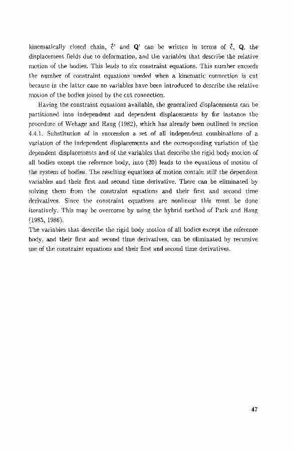
kinematically closed chain, c' and Q' can be written in terms of c, Q, the
displacement fields due to deformation, and the variables that describe the relative
motion of the bodies. This leads to six constraint equations. This number exceeds
the number of constraint equations needed when a kinematic conneetion is cut
because in the latter case no variables have been introduced to describe the relative
motion of the bodies joined by the cut connection.
Having the constraint equations available, the generalized displacements can be
partitioned into independent and dependent displacements by for instanee the
procedure of Wehage and Haug (1982), which has already been outlined in section
4.4.1. Substitution of in Succession a set of all independent combinations of a
varlation of the independent displacements and the corresponding varlation of the
dependent displacements and of the variables that describe the rigid body motion of
all bodies except the reference body, into (20) leads to the equations of motion of
the system of bodies. The resulting equations of motion contain still the dependent
variables and their first and second time derivative. These can be eliminated by
solving them from the constraint equations and their first and second time
derivatives. Sirree the constraint equations are nonlinear this must be done
iteratively. This may be overcome by using the hybrid methad of Park and Haug
(1985, 1986).
The variables that describe the rigid body motion of all bodles except the reference
body, and their first and second time derivatives, can be eliminated by recursive
use of the constraint equations and their first and second time derivatives.
47

chapter 5
Assessment of descriptions and approximations
5.1 Introduetion
In this chapter miscellaneous topics related to the analysis of the dynamic
behaviour of systems of deformable boclies are considered. In section 5.2 possible
savings of computation time by using base functions for approximating the
displacement field due to deformation that satisfy the mean displacement
condi1iions (2.8) and (2.10) are investigated. The finite element method and the
modal synthesis metbod are considered insection 5.3 and 5.4, respectively. Special
attention is paid to preventing rigid body motions in the displacement field due to
deformation. The effect of the frequently used lumped mass approximation is
considered in section 5.4. In section 5.5 the influence of nonlinearities going with
the displacement field due to deformation are considered. A procedure for
correcting eigenfrequencies going with base functions that do not agree with the
actual eigenfrequencies is presented in section 5.6. This procedure is used for
alleviating the integration time step reducing effect of high frequencies.
The numerical examples presented in this chapter are carried out with the
version of DADS (CADSI, 1988) for three-dimensional problems on a VAX 8530.
The required CPU time for a specific problem depends on several input parameters.
The reported CPU times apply for default values of the error tolerances, only
binary output, no reaction forces, and a maximum integration time step size which
is equal to the print interval.
5.2 Mean displacement conditions
In order to investigate possible merits of using base functions that satisfy the mean
displacement conditions (2.8) and (2.10), the slider-crank mechanism shown in fig.
5.1 is analyzed. lt consists of a rigid crank with length 0.15 m, a deformable
connecting rod, and a rigid sliding block with mass equal to half the mass of the
connecting rod. The connecting rod has a length t 0.3 m and a circular cross
section with diameter d 0.006 m. It is made of steel with a modulus of elasticity
E = 0.2*1012 N/m2 and a mass density p = 7.87*103 kgfm3• Axial deformation of
the connecting rod is neglected. The crank rotates with a constant angular velocity
fl = 150.0 radfs. In the initia! configuration, the connecting rod is straight and it is
48
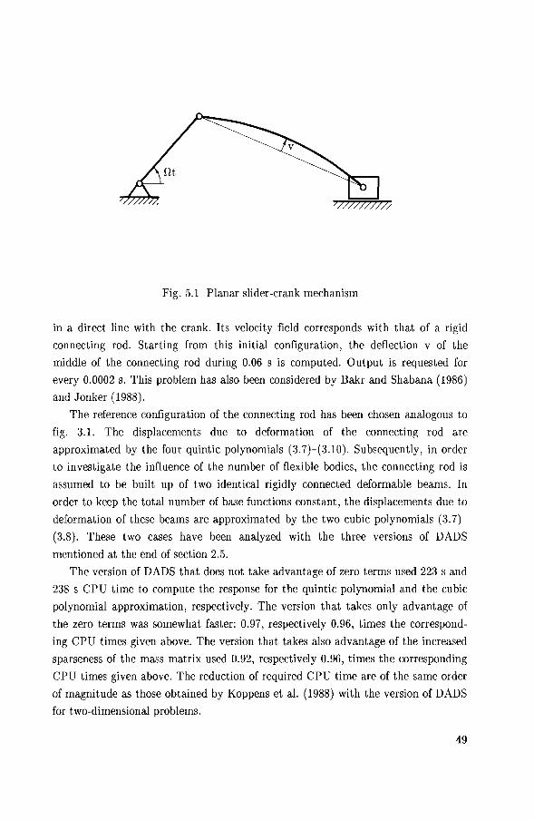
Fig. 5.1 Planar slider-crank mechanism
in a direct line with the crank. lts velocity field corresponds with that of a rigid
connecting rod. Starting from this initial configuration, the deflection v of the
middle of the connecting rod during 0.06 s is computed. Output is requested for
every 0.0002 s. This problem has also been considered by Bakr and Shabana (1986)
and Jonker (1988).
The reference configuration of the connecting rod has been chosen analogous to
fig. 3.1. The displacements due to deformation of the connecting rod are
approximated by the four quintic polynomials (3. 7)-(3.10). Subsequently, in order
to investigate the influence of the number of flexible bodies, the connecting rod is
assumed to be built up of two identical rigidly connected deformable beams. In
order to keep the total number of base functions constant, the displacements due to
deformation of these beams are approximated by the two cubic polynomials (3. 7)(3.8). These two cases have been analyzed with the three versions of DADS
mentioned at the end of section 2.5.
The version of DADS that does not take advantage of zero terms used 223 s and
238 s CPU time to compute the response for the quintic polynomial and the cubic
polynomial approximation, respectively. The version that takes only advantage of
the zero terms was somewhat faster: 0.97, respectively 0.96, times the conespond
ing CPU times given above. The version that takes also advantage of the increased
sparseness of the mass matrix used 0.92, respectively 0.96, times the conesponding
CPU times given above. The reduction of required CPU time are of the same order
of magnitude as those obtained by Koppens et al. (1988) with the version of DADS
for two-dimensional problems.
49

.02.---~.-----.-----~----~----.---~
-------- cubic
----- quintic .01
v/1
.0
-.01
.0 1f 2fl' CRANK ANGLE (rad}
Fig. 5.2 Assumed modes solution using cubic and quintic polynomials
In fig. 5.2 the dimensionless deflection v / t of the middle of the connecting rod is
plotted versus the angle over which the crank has rotated. The response related to
the quintic polynomial approximation deviates from the response conesponding to
the cubic polynomial approximation. This can be attributed to nonlinearities which
are taken into account for the cubic polynomial approximation because the connect
ing rod bas been modelled as two rigidly connected beams as will be explained in
section 5.5. The response conesponding to the cubic polynomial approximation is
indistinguishable from the linear solution obtained by Jonker (1988).
The above slider-crank mechanism is actually a two-dimensional mechanism. A
three-dimensional slider-crank mechanism is considered by Jonker (1988) (cf. fig.
5.3). It has the same dimensions and initia! configuration as the above slider-crank
mechanism.
The reference configuration of the connecting rod bas been chosen analogous to
fig. 3.1. The displacements due to deformation of the connecting rod are approxi
mated by the four quintic polynomials (3.7)-(3.10) and the conesponding four
quintic polynomials for displacements in the êa direction. The connecting rod has
also been divided into two identical rigidly connected deformable beams. The
displacements due to deformation of these beams are approximated by the two
cubic polynomials (3.7)-(3.8) and the corresponding two cubic polynomials for the
displacements in the êa direction. These two cases have been analyzed with the
three versionsof DADS mentioned at the end of section 2.5.
50

Ie, revolute joint"-
~ l n spherical joint
Fig. 5.3 Spatial slider-crank mechanism
The version of DADS that doesnottake advantage of zero terms required 1016 s
and 1224 s CPU time to compute the response for the quintic polynomial and the
cubic polynomial approximation, respectively. The version that takes only
advantage of the zero terms was somewhat faster: 0.99, respectively 0.98, times the
conesponding CPU times given above. The version that takes also advantage of the
increased sparseness of the mass matrix used 0.83, respectively 0.82, times the
conesponding CPU times given above.
Fig. 5.4 shows the components in ê2 and e3 direction of the dimensionless
deflection of the middle of the connecting rod versus the crank angle. The deviation
of the responses going with the quintic polynomial approximation and the cubic
polynomial approximation can be attributed to nonlinearities which are taken into
account for the cubic polynomial approxirnation because then the connecting rod is
modelled as two rigidly connected beams. The two-beams salution is close to the
nonlinear salution obtained by Jonker (1988). The difference is of the sameorder of
magnitude as the difference shown in fig. 5.4.
From the above results it can be concluded that only a small reduction of
required CPU time is obtained when advantage is taken of zero terms. This
reduction becomes larger when the number of assumed displacement fields is
increased. For a small number of assumed displacement fields, the saving of
computation time is obtained from evaluating the equations of motion; for a large
number of assumed displacement fields the time-saving is obtained from solving the
equations of motion.
51
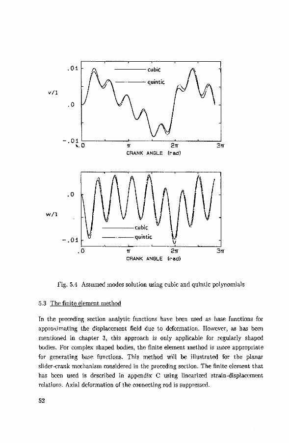
v/1
w/1
.01 ----cubic
.0
-.01L--~----~----~----~--~----~
"· 0 1f 211"
.0
-.01
.0
3'!1" CRANK ANGLE (rad)
---.--quintic
1f 211" 3'!1" CRANK ANGLE (rad)
Fig. 5.4 Assumed modes solution using cubic and quintic polynomials
5.3 The finite element metbod
In the preceding section analytic functions have been used as base functions for
approximating the displacement field due to deformation. However, as has been
mentioned in chapter 3, this approach is only applicable for regularly shaped
bodies. For complex shaped bodies, the finite element method is more appropriate
for generating base functions. This method will be illustrated for the planar
slider-crank mechanism considered in the preceding section. The finite element that
has been used is described in appendix C using linearized strain-displacement
relations. Axial deformation of the connecting rod is suppressed.
52

v/1
.02~--~-----r----.-----.----,----,
.01
.0
-.01
.0
--·---1 element
· · · · · · · · · · · 2 elements ----3 & 4 elements
1't 21't CRANK ANGLE (rad)
Fig. 5.5 Finite element solution: simply supported conditions
Fig .. 5.5 shows the dimensionless deflection vjt of the middle of the connecting
rod for the case in which rigid body motions of the displacement field due to
deformation are prevented by prescrihing the deflection of the endpoints of the
connecting rod. This case h&'l been analyzed with the connecting rod divided into
one, two, three, and four elements, respectively. The solutions for the three- and
four-element subdivision are indistinguishable which indicates that a converged
solution has been abtairred for the three-element subdivision. This solution is
indistinguishable from the quintic polynomial salution presented in the preceding
section. The CPU times required for obtaining the salution for the one-, two-,
three-, and four-element subdivision are respectively, 86 s, 283 s, 683 s, and 1455 s.
The planar slider-crank mechanism has also been analyzed for the case in which
rigid body motions of the displacement field due to deformation are prevented by
prescrihing the deflection and the rotation of the endpoint of the connecting rod
that is attached to the crank. (This may seem an odd choice. However, it simplifies
formulating the constraint equations of two interconnected bodies because the
displacements due to deformation of just one body are involved. In fact, this is used
in formulating the equations of motion by the computer programs TREETOPS and
CONTOPS (Singh et al. (1985, 1986)). This case has been analyzed with the
connecting rod divided into one, two, three, and four elements, respectively. Fig.
5.6 shows the dimensionless deflection v / t of the middle of the mnnecting rod. The
solutions obtained for the three- and four-element subdivision are indistinguishable
which indicates that a converged solution has been obtained for the three-element
53

v/1
.04
.02
.0
-.02
.0
---·--1 element
· · · · · · · · · · · · · · 2 elements -----3 & 4 elements
211 CRANK ANGLE (rad)
Fig. 5.6 Finite element solution: one-sided built in conditions
subdivision. The CPU time required for obtaining the salution for the one-, two-,
three-, and four-element subdivision are respectively, 81 s, 244 s, 580 s, and 1294 s.
The results shown in fig. 5.5 and fig. 5.6 differ. The slider"crank mechanism is
too complex to trace the cause of this discrepancy. For this reasou the deformable
beam shown in fig. 5. 7 is considered. This beam and the connecting rod of the
slider-crank mechanism are identical. In the initial configuration the beam is
straight and its velocity is zero. The beam will bend under the action of gravity.
The displacement field due to deformation is approximated with three finite
elements using linearized strain-displacement relations. Rigid body motions of the
displacement field due to deformation are prevented by prescrihing either both
endpoint deflections or the deflection and the rotation of the left endpoint. Three
values of the axial force F are considered: F 0 N, F -200 N, and F = 200 N.
(The order of magnitude of the axial force in the connecting rod of the slider-crank
mechanism is 102 N.)
F F • •
Fig. 5. 7 Simply supported beam
54

v/1 F = -200 N
F = 0 N
1.0 F = 200 N
.0
.0 .01 .02 .03 TIME {s)
Fig. 5.8 Deflection of simply supported beam: one-sided built in conditions
Fig. 5.8 shows the dimensionless deflection vjt of the middle of the beam for the
above three values of the axial force F in case the deflection and the rotation of the
left endpoint are prescribed. The mean value of the dimensionless deflection for
F = 0 N agrees with the dimensionless static deflection of the beam:
(v8/t) = (5/24)pt3g/Ed2 60.3*10-6. The period of the response agrees with the
analytic value of the period going with the lowest natura! frequency of the beam:
Ta= (8f';r)(t2/d).fii{E 7.58*10-3 s. The deflection and the period become smaller
when a compressive load (F = -200 N) is applied, whereas the deflection and the
period increase when a tensile load (F = 200 N) is applied! This is opposite to what
happens in reality. This can be explained with the help of fig. 5.9. It shows the
beam in a deflected configuration, and the reference configuration of the beam after
a rigid body motion which corresponds to this deflected configuration. Forces
normal to this reference configuration cause a deflection of the beam. The applied
force F has a component normal to this reference configuration. For a positive value
of F, this component wil! increase the deflection of the beam; for a negative value of
F, this component will decrease the deflection of the beam. This agrees with the
numerical results presented in 5.8. For small deflections of the beam, the
component of the applied force normal to the reference configuration is proportional
to this deflection. Consequently it behaves as if it arises from a linear spring with a
negative stiffness coefficient for a positive value of F, and a positive stiffness
coefficient fora negative value of F. This explains the change in eigenfrequency due
to the application of an axial force.
55

---- -- ..... ......
Fig. 5.9 Components of the axialload parallel and normal to the
reference configuration
All this does not happen when the beam is analyzed with rigid body motions of
the displacement field due to deformation eliminated by prescrihing the deflection
of the endpoints of the beam, because in that case the axial force is parallel to the
reference configuration. This is confirmed by the results obtained for the case with
prescribed endpoint deflections which are for all three values of F identical to the
above result for F 0 N.
From this result, it may be expected that the results for the slider-crank
mechanism for both sets of conditions will agree better in case the axial forc~ is
smaller. This will be the case when the slider is lighter. In order to verify this
anticipation, the slider-crank mechanism is analyzed with a slider mass equal to
zero. The results for both sets of conditions are shown in fig. 5.10. It can be seen
that the results agree much better, which supports the above explanation.
.02 ----- simply supported
--·--cantilever
.01 v/1
.0
-.01
.0 11 311
CRANK ANGLE {rad}
Fig. 5.10 Finite element solution: slider mass equal to zero
56

Another numerical experiment reveals an interesting phenomenon. The rigid ->
body properties m, C1 and C3 of the connecting rod are set equal to zero, and a
rigid body with mass properties identical to those of the connecting rod is rigidly
attached to the connecting rod at the endpoint with prescribed deflection and
rotation. The results obtained for this problem are indistinguishable from those
obtained with prescribed endpoint deflection and rotation, which indicates that
these two problems are identicaL The forces that are necessary for the motion of
the extra body are reacted by a concentrated force and moment at the endpoint of
the connecting rod. Since both problems are identical, this occurs also wherr rigid
body motions are prevented by prescrihing endpoint deflection and rotation of the
connecting rod. Sirree in reality there is no concentrated moment at the end of the
connecting rod, this may lea.d to incorrect results.
5.4 The modal synthesis metbod
From the CPU times reported in the preceding section it can be concluded that the
CPU time required for a finite element analysis is about directly proportional to the
square of the number of degrees of freedom. A regularly shaped body such as the
connecting rod does not need to be divided into many elements. However, complex
shaped boclies must be divided into many elements in order to be able to describe
the shape of the body sufficiently accurate. The salution of the conesponding
equations of motion requires much computation time. Therefore it is desirabie to
reduce the number of degrees of freedom in order to shorten the required
computation time. The modal synthesis methad can be used for this purpose. The
effectiveness of the modal synthesis method depends to a great extent on a proper
choice of base functions for approximating the displacement field due to
deformation. Considerations that lead to a specific choice of base functions are
given in subsection 5.4.1 for the planar slider-crank mechanism. In subsection 5.4.2
the conditions that are used for eliminating rigid body motions are considered. An
approximate metbod for obtaining the time-independent inertia coefficients (2.34)
(2.41), the lumped mass approximation, is investigated in subsection 5.4.3.
5.4.1 Selection of base functions
In selecting base functions for the connecting rod, the forces that cause the
deformation must be considered. In order to identify the importance of different
farces causing the deformation, fig. 5.11 gives the total deflection of the middle of
the connecting rod obtained with three finite elements (cL fig. 5.5), and the quasi-
57

.02~--~r----,----~----~-----r----~
------finite elements (fig. 5.5)
---·--- elastodynamic .01
v/1
.0
-.01
.0 CRANK ANGLE (red)
Fig. 5.11 Deflection of the middle of the connecting rod
static deflection resulting from the inertia load and the corresponding reaction
forces at the endpoints of the connecting rod that go with the motion which follows
from a kinematic analysis of the corresponding slider-crank mechanism with a rigid
connecting rod (elastodynamic deflection, cf. appendix D). It can beseen that the
main contribution can be attributed to the load arising from the rigid body motion
of the connecting rod. This inertia load is a distributed load varying linearly along
the axis of the connecting rod as bas been mentioned already in section 3.2. It can
be subdivided into a eonstant distributed load and a linearly distributed load that
is antisymmetrie relative to the middle of the connecting rod (fig. 5.12). The
deflection of the middle of the connecting rod due to the antisymmetrie load is zero.
Consequently only the deflection resulting from the uniform load is of interest when
one is concerned with the deflection of the middle of the connecting rod. The slider
crank mechanism has been analyzed using the deflection of the connecting rod
+
Fig. 5.12 Resolution of load into symmetrie and antisymmetrie component
58
resulting from a uniform load as base function for the connecting rod. This
displacement field has been determined using a four-element subdivision. The
response obtained with this displacement field is indistinguishable from the
response obtajned with the connecting rod divided into three finite elements.
However, the required CPU time equals 59 s which is only 0.09 times the CPU time
used for the finite element analysis with three elements. The rednetion is even
larger when the CPU time used for the modal synthesis analysis is compared with a
finite element analysis without constraining the axial deformation of the connecting
rod: the required CPU time for the modal analysis amounts then 0.02 times the
required CPU time for the finite element analysis. It is more precise to sustain the
latter rednetion because modes of deformation cannot be readily eliminated from a
finite element model. From this result it can be concluded that a substantial
rednetion of required CPTJ time can be obtained with the modal synthesis method.
A significant portion of the response of the connecting rod arises from its
fundamental eigenfunction. The result obtained with just the static displacement
field of the connecting rod resulting from a constant distributed load is so close to
the total response because this displacement field is close to its fundamental
eigenfunction. The magnitude of the contribution of the fundamental eigenfunction
is determined by the exciting load, and the initial displacement field due to
deformation and the conesponding velocity field of the connecting rod. The main
exciting load consists of the inertia load and the corresponding reaction forces at
the endpoints of the connecting rod that go with the rigid body motion of the
connecting rod. The response due to this exciting force will be close to the quasi
static response, because the main frequency of the excitation (0 = 150.0 radjs) is
well below the fundamental frequency of the connecting rod
(v = ( ilj4)(djt2).fETii 829.2 rad/s). For this reason the portion of the response
of the connecting rod going with the fundamental eigenfunction is mainly due to the
initia! displacement field due to deformation and the conesponding velocity field of
the connecting rod. The initia! conditions used in the above analysis are not
realistic. This follows also from experimental results presented by Sung et al.
(1986). The influence of initia! conditions will fade away due to damping and the
response will become nearly periodic in process of time. Such a periodic response
wil! be obtained immediately when the analysis is started using proper initial
conditions. It may be expected that these initia! conditions wil! be close to the
conditions which follow from a quasi-static analysis. From a quasi-static analysis
follows that the initia! deflection of the middle of the connecting rod equals 0 m,
and the initia! velocity equals (15/128)p03t 5jEd2 = 1.05 mjs (cf. D.ll). Fig. 5.13
59
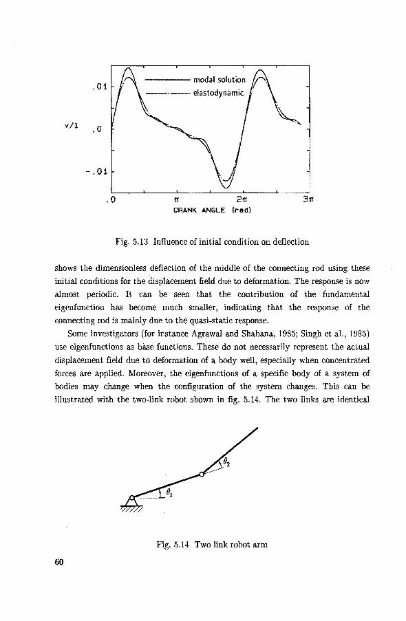
.01 ---- modal solution
v/1 .o
-.01
.0 1f 21f
CRANK ANGLE (rad)
Fig. 5.13 Influence of initial condition on deflection
shows the dimensionless deflection of the middle of the connecting rod using these
initial conditions for the displacement field due to deformation. The response is now
almost periodic. It can be seen that the contribution of the fundamental
eigenfunction has become much smaller, indicating that the response of the
connecting rod is mainly due to the quasi-static response.
Some investigators (for irtstance Agrawal and Shabana, 1985; Singh et al., 1985)
use eigenfunctions as base functions. These do not necessarily represent the actual
displacement field due to deformation of a body well, especially when concentrated
forces are applied. Moreover, the eigenfm1ctions of a specific body of a system of
bodies may change when the configuration of the system changes. This can be illustrated with the two-link robot shown in fig. 5.14. The two links are identical
Fig. 5.14 Two link robot arm
60

------02 0
---------02= 7r
/ /
/ 2 /
Fig. 5.15 Eigenfunctions of inner link
with the exception of the bending stiffness which is assumed to be infinite for the
outer link. The angles e1 and e2 are kinematically driven. Consider the cases with e1
constant, and fh = 0, respectively 82 = 1r.
Fig. 5.15 shows the first and second eigenfunction of the inner link for these two
situations. It can be seen that especially the second eigenfunction depends on the
configuration of the robot arm. This example illustrates that it may be difficult to
decide which eigenfunctions should be used.
However, it is not difficult to decide which static displacement fields will
describe the actual displacement field of the inner link probably wel!. The outer
link applies a force and a moment to the inner link. Consequently the two static
displacement fields resulting from either a concentrated force or a moment applied
at the endpoint of the inner link will probably be a good approximation of the
displacement field of the inner link. In any case they describe the quasi-static
deflection due to the force and moment from the outer link exactly.
Fig. 5.16 shows the approximated eigenfunctions of the inner link for ez = 0
using the above suggested base functions. The fundamental eigenfunction is
indistinguishable from the exact eigenfunction. The second eigenfunction is close to
the exact eigenfunction. The approximated eigenfunctions for fh 1r are indistin
guishable from the corresponding exact eigenfunctions. Consequently the above
suggested base functions give also a good approximation of the dynamic behaviour
of the inner link.
The load applied to a specific body should be considered in selecting base
functions for approximating its displacement field. One should consider to use also
eigenfunctions as base functions in case the frequency of the excitation is close to an
eigenfrequency of the body.
61

----eigenfunction
-- ---approximation
Fig. 5.16 Approximated eigenfunctions of the inner link for ()2 0
5.4.2 Elimination of rigid body motions
The base function used in the above analysis of the slider-crank mechanism does
not contain a rigid body motion because the deflections at the endpoints of the
connecting rod are equal to zero. The results obtained with the finite element
metbod are incorrect in case rigid body motions are prevented by prescrihing the
endpoint deflection and rotation of the connecting rod as has been discussed in
section 5.3. In order to investigate whether this is also the case when the modal
synthesis metbod is used, the planar slider-crank mechanism is analyzed using
eigenfunctions of the connecting rod going with zero deflection and rotation of the
endpoint that is attached to the crank.
Fig. 5.17 shows the dimensionless deflection of the middle of the connecting rod in case two, respectively three eigenfunctions are used as base functions. These
eigenfunctions have been determined with the connecting rod divided into four
finite elements. The solid curve is the response obtained with the finite element
metbod using a three-element approximation with rigid body motions eliminated by
prescrihing the endpoint deflection and rotation (cf. fig. 5.6). lt can be concluded
that the solution using the eigenfunctions of the cantilever connecting rod converges
to this finite element solution when the number of eigenfunctions is increased.
Consequently, the model using eigenfunctions suffers from the same problems as the
fini te element model.
Agrawal and Shabana (1985) obtained simHar results in case they approximated
the displacement field due to deformation with eigenfunctions of the cantilever
connecting rod. They attributed these incorrect results to the fact that these
eigenfunctions poorly represent the deflected shape of the connecting rod. In order to show that this explanation is incorrect, the conditions that are used for
eliminating rigid body motions are changed. This is done by adding small rigid
body motions to the original base functions. This transformation does not change
62
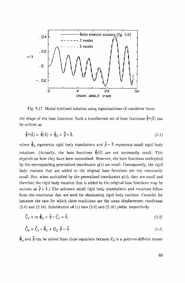
.04 ---- finite element solution (fig. 5.6)
------2 modes
.......... 3 modes .02
v/1
.0
-.02
.0 2'11' CRANK ANGLE (rad)
Fig. 5.17 Modal synthesis solution using eigenfunctions of cantilever beam
the shape of the base functions. Such a transformed set of base functions ~*(x) ca.n
be written a.s
.... ... ... ... .... .... ... tg*(x) p(x) + Po+ 1} x x, (5.1)
where ~0 represents rigid body tra.nsla.tions a.nd ~ x x represents small rigid body
rota.tions. (Actua.lly, the base functions ~(x) are not necessarily small. This
depends on how they have been normalized. However, the base functions multiplied
by the conesponding generalized coordinates {t( t) are sma.ll. Consequently, the rigid
body motions that are added to the original base functions are not necessarily
sma.ll. But, when multiplied by the genera.lized coordinates q(t), they aresmalland
therefore the rigid body rotation that is added to the original base functions may be
written as ~ x x.) The unknown small rigid body translations and rotations follow
from the conditions that are used for eliminating rigid body motions. Consider for
instanee the case for which these conditions are the mean displacement conditions
(2.8) and (2.10). Substitution of (1) into (2.8) and (2.10) yields, respectively
.. 0, (5.2)
.. 0. (5.3)
.. .. Po and 1} can be solved from these equations because C3 is a positive-definite tensor
63

--· ---fundamental eigenfunction
----- modified eigenfunction _ _...-_ _...-
. ...---------~---
Fig. 5.18 Fundamental and modified eigenfunction of cantilever beam
(it is the inertia tensor of the body in the reference configuration). Substitution of
the result into (1) yields the modified base functions. Fig. 5.18 shows the
fundamental eigenfunction of the cantilever connecting rod and the base function
that is obtained using the above transformation.
The slider-crank mechanism has been analyzed using eigenfunctions of the
connecting rod going with zero deflection and rotation of the endpoint that is
attached to the crank after the above described transformation. The deflection of
the middle of the connecting rod obtained with two, respectively three of such base
functions is given in fig. 5.19 . The solid curve is the response obtained with the
finite element method using a three-element approximation with rigid body motions
eliminated by prescrihing the deflection of the endpoints of the connecting rod ( cf.
.02,--~---r---~----r---~----~
----- finite element solution (fig. 5.5)
- --- --2 modes .01
• • · • • • • • · 3 modes
v/1
.0
-.01
.0 21Y CRANK ANGLE [rad)
Fig. 5.19 Modal synthesis solution using modified eigenfunctions of cantilever beam
64
fig. 5.5). It can be seen that the salution obtained with modified eigenfunctions
converges to this finite element solution.
This leads to the condusion that the solution obtained with eigenfunctions of
the cantilever connecting rod converges also to the correct salution provided
suitable conditions are used for eliminating rigid body motions. However, when
compared with the static deflection mode used in the beginning of this section,
more base functions are needed because the eigenfunctions of the cantilever
connecting rod do represent the deflected shape of the connecting rod worse.
5.4.3 Lumped mass approximation
In the preceding part of this section, the time-independent inertia coefficients
(2.34)-(2.41) have been assembied from the conesponding coefficients of the beam
element, which have been evaluated analytically. In literature a lumped mass
approximation is frequently used (Sunada and Dubowsky, 1981, 1983; Yoo and
Haug, 1986a, 1986b). The advantage of that approach is that the time-independent
coefficients can be computed from nodal displacements and nodal masses which can
be determined with a standard finite element computer program. It may be
expected that a lumped mass approximation is less accurate than a consistent mass
approximation. In order to evaluate the consequences of using a lumped mass
approximation, the planar slider-crank mechanism of fig. 5.1 is considered. The
displacement field due to deformation is approximated with the static displacement
field resulting from a uniform load that has been used in subsection 5.4.1.
From subsection 5.4.1 it can be concluded that a fom-element subdivision of the
connecting rod yields a sufficiently accurate base function and conesponding time
independent inertia coefficients when a consistent mass approximation is used. Fig.
5.20 shows the dimensionless deflection of the middle of the connecting rod in case a
lumped mass approximation is used. The results are obtained in case the base
function is obtained with a four-element subdivision and a.n eight-element
subdivision, respectively. The result going with the eight-element subdivision is
indistinguishable from the result obtained with the three-element subdivision shown
in fig. 5.5. The computation of the response going with a four-element subdivision
and an eight-element subdivision took 59 s, respectively 62 s CPU time.
From these results it can be concluded that when compared with the consistent
mass approximation, the lumped mass approximation may require a finer
subdivision into elements for determining base functions in order to obtain the
corresponding time-independent coefficients sufficiently accurate. This is not a
severe dismerit because the bodies encountered in practice have generally a complex
65
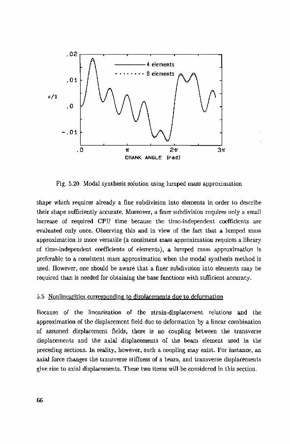
.02.----.-----.----.-----.----,.----,
----4 elements
• · · · · · · · 8 elements .01
v/1
.0
-.01
.0 211" 311" CRANK ANGLE (rad)
Fig. 5.20 Modal synthesis solution using lumped mass approximation
shape which requires already a fine subdivision into elements in order to describe
their shape sufficiently accurate. Moreover, a finer subdivision requires only a small
increase of required CPU time because the time-independent coefficients are
evaluated only once. Observing this and in view of the fact that a lumped mass
approximation is more versatile (a consistent mass approximation requires a library
of time-independent coefficients of elements), a lumped mass approximation is
preferabie to a consistent mass approximation when the modal synthesis methad is
used. However, one should be aware that a finer subdivision into elements may be
required than is needed for obtaining the base functions with sufficient accuracy.
5.5 Nonlinearities conesponding to displacements due to deformation
Because of the linearization of the strain-displacement relations and the
approximation of the displacement field due to deformation by a linear combination
of assumed displacement fields, there is no coupling between the transverse
displacements and the axial displacements of the beam element used in the
preceding sections. In reality, however, such a coupling may exist. For instance, an
axial force changes the transverse stiffness of a beam, and transverse displacements
give rise to axial displacements. These two items will be considered in this section.
66
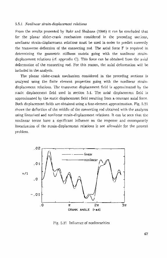
5.5.1 Nonlinear strain-displacement relations
From the results presented by Bakr and Shabana (1986) it can be concluded that
for the planar slider-crank mechanism considered in the preceding sections,
nonlinear strain-displacement relations must be used in order to predict correctly
the transverse deflection of the connecting rod. The axial force F is required in
determining the geometrie stiffness matrix going with the nonlinear strain
displacement relations ( cf. appendix C). This force can be obtained from the a,xial
deformation of the connecting rod. For this reason, the a,"i:ial deCormation wil! be
included in the analysis.
The planar slider-crank mechanism considered in the preceding sections is
analyzed using the finite element properties going with the nonlinear strain
displacement relations. The transverse displacement field is approximated by the
static displacement field used in section 5.4. The axial displacement field is
approximated by the static displacement field resulting from a constant axial force.
Both displacement fields are obtalned using a four-element approximation. Fig. 5.21
shows the deflection of the middle of the conm~cting rod obtained with the analyses
using linearized and nonlinear strain-displacement relations. It can be seen that the
nonlinear terms have a significant influence on the response and consequently
linearization of the strain-displaeement relations is not allmvabie for the present
problem.
. 02 r-----.-----.---.----.----..,----,
--· --linear
. 01
v/1
.0
-.01
.0 2tr CRANK ANGLE (rad)
Fig. 5.21 Influence of nonlinearities
67

The linear solution obtained for the case in wbich tbe connecting rod is divided
into two identical beams using a cubic polynornial approximation of the displace
ment field due to deformation (cf. fig. 5.2) is close to the nonlinear solution shown
in fig. 5.21. This can be explained with the help of fig. 5.22. It shows a current
configuration of the connecting rod (solid curve), and the reference configuration
after the rigid body motion corresponding to this current configuration ( dasbed
lines). The difference between these configurations represents displacements due to
deformation. These are mucb smaller when the connecting rod is divided into two
beams. Consequently, linearization of strain-displacement relations is allowable for
much larger deflections of the connecting rod in case it is approximated witb a
number of beams. However, then it is not possible to reduce the number of degrees
of freedom using the modal synthesis method. Because of the required computation
time, an analysis based on the modal synthesis metbod combined witb nonlinear
strain-displacement relations is preferabie to an analysis based on dividing the
connecting. rod into a number of beams combined witb linearized strain
displacement relations.
one-beam approximation
two-beams approximation
Fig. 5.22 Displacements due to deformation when tbe connecting
rod is divided into several beams
5.5.2 Nonlinear combinations of assumed displacement fields
The displacement field due to deformation bas been approximated by a linear
combination of assumed displacement fields (cf. 2.28). However, it may he
necE>.ssary to include also nonlinear terms in order to predict the dynamic bebaviour
of bodies correctly. Tbis may be the case for instanee for rotating beams.
68
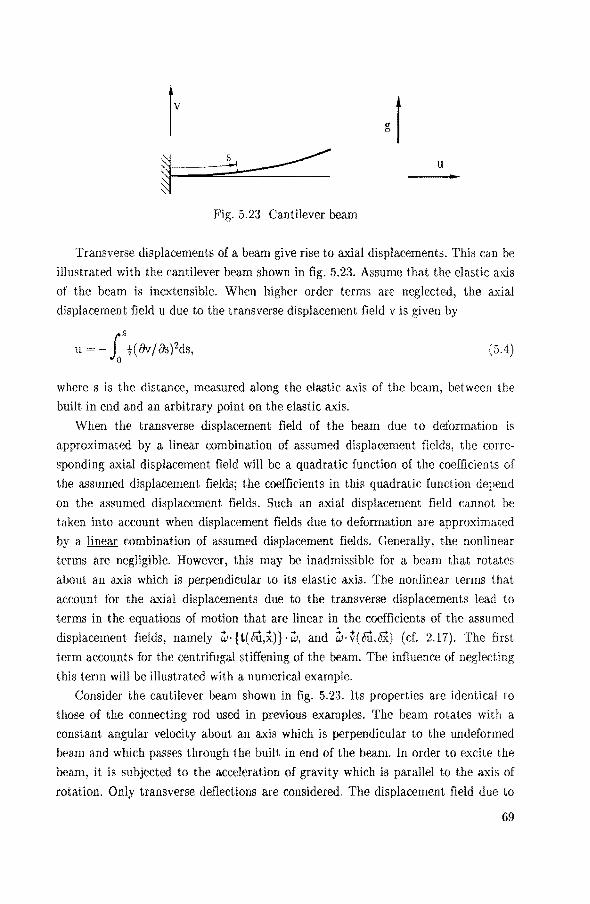
u
Fig. 5.23 Cantilever beam
Transverse displacementsof a beam give rise to a.xial displacements. This can be
illustrated with the cantilever beam shown in fig. 5.23. Assume that the elastic a.xis
of the beam is inextensible. When higher order terms are neglected, the a.xial
displacement field u due to the transverse displacement field v is given by
U= (5.4)
where s is the distance, measured along the elastic a.xis of the beam, between the
built in end and an arbitrary point on the elastic a.xis.
When the transverse displacement field of the beam due to deformation is
approximated by a linear combination of assumed displacement fields, the corre
sponding a.xial displacement field will be a quadratic function of the coefficients of
the assumed displacement fields; the coefficients in this quadratic function depend
on the assumed displacement fields. Such an ax.ial displacement field cannot be
taken into account when displacement fields due to deformation are approximated
by a combination of assumed displacement fields. Generally, the nonlinear
terms are negligible. However, this may be inadmissible for a beam that rotates
about an a.xis which is perpendicular to its elastic a.xis. The nonlinear terms that
account for the a.xial displacements due to the transverse displacements lead to
terms in the equations of motion that are linear in the coefficients of the assumed
displacement fields, namely w· { t( ÓÛ,x)} · w, and ~. v( ÓÛ,bX) ( cf. 2.17). The first
term accounts for the centrifugal stiffening of the beam. The influence of neglecting
this term will be illustrated with a numerical example.
Consider the cantilever beam shown in fig. 5.23. lts properties are identical to
those of the connecting rod used in previous examples. The beam rotates with a
constant angular velocity about an a.xis which is perpendicular to the undeformed
beam and which passes through the built in end of the beam. In order to excite the
beam, it is subjected to the acceleration of gravity which is parallel to the a.xis of
rotation. Only transverse deflections are considered. The displacement field due to
69

deforma.tion is a.pproxima.ted by the eigenfunctions corresponding to the cantilever
bea.m. Analyses for several valnes of the a.ngula.r velocity show no dependency of the
response on the angula.r velocity which ca.n be attributed to the missing of the
centrifugal stiffening term.
This failure may be partially obviated by cha.nging the conditions for eliminat
ing rigid body motions in the displacement field due to deformation such tha.t the
rigid body motion going with a deflection of the bea.m cause displacements towards
the a.xis of rotation. This ma.y be achieved for instanee by cha.nging to the mea.n
axis conditions using eqs. (5.1)-(5.3). Fig. 5.24 shows the displacement of the 'free
end of the beam parallel to the axis of rotation for an angular velocity of 150.0
rad/s (dashed curve). It has been obtained with the two lowest eigenfunctions of
the cantilever beam transformed according to eqs. (5.1)-(5.3). Increasing the
number of assumed displacement fields does not change the response, which
indicates that a converged solution is obtained for two assumed displacement fields.
The dot and clash curve represents the response obtained in case the two lowest
eigenfunctions of the cantilever bea.m are used. Comparison of the two curves shows
that the eigenfrequency is higher and the deflection is smaller when the tra.nsformed
eigenfunctions are used. This is what should happen when the beam rotates.
Linearized strain-displa.cement relations have been used for the above-described
analysis. Consequently, the stiffening of the beam due to a.n a.xial tensile force is
not taken into account. In order to study the influence of this force, the rotating
beam has also been a.nalyzed using nonlinea.r strain-displacement relations. The
a.xial force, which is required for determining the geometrie stiffness matrix ( cf. *E -3
.-----~----~----~-----r-----r----~
v/1
1.0 eigenfunctions
modified
.5 nonlinear
3 beams
.0
.o .02 .04 .06
TIME (s)
Fig. 5.24 Deflection of the endpoint of the rotating beam
70
appendix C), is obtained from the axial deformation of the beam. For this purpose,
an extra assumed displacement field is used which represents the quasi-static
displacement field of the beam resulting from the inertia forces which arise from a
rotation of the beam in case it is undeformed. The response of the endpoint of the
beam for this approximation is given by the solid curve in fig. 5.24. As can be seen
it is not allowable to use linearized strain-displacement relations for this problem.
Another way to obviate the absence of quadratic terms in the displacement field
due to deformation is to divide the beam into a number of parts. As has been
mentioned in the preceding subsection, the displacements due to deformation are
then much smaller. Hence, also the conesponding axial displacements due to the
transverse displacements will be much smaller and are consequently negligible for
much larger deflections. The rotating beam has been approximated by dividing it
into three identical parts. The displacements due to deformation of these parts are
approximated by the cubic polynomials (3. 7)-(3.8). The response obtained for this
approximation is given by the dotted curve of fig. 5.24. As can be seen the
agreement between the three beam approximation and the approximation obtained
with the transformed eigenfunctions using nonlinear strain-displacement relations is
good.
Terms in the equations of motion that are linear in the displacements due to
deformation are discarded due to the approximation of the displacement field due
to deformation by a linear combination of a set of assumed displacement fields. For
a rotating beam, the influence of these terms is taken into account when use is
made of nonlinear strain-displacement relations and assumed displacement fields
that satisfy the mean displacement conditions. More research is necessary to find
out whether this holds more generally. When this is not the case, also nonlinear
terms must be included for the approximation of displacement fields due to defor
mation.
5.6 Shifting of frequencies
5.6.1 Tuning of frequencies
One is often more concerned with the dynamic behaviour of the system of bodies as
a whole rather than with the displacement field of the individual bodies. The
displacements of the points of the bodies that are connected to other bodies should
be approximated well in order to have a good approximation of the global motion of
the system of bodies. Due to the connections, concentrated loads act on the bodies
71
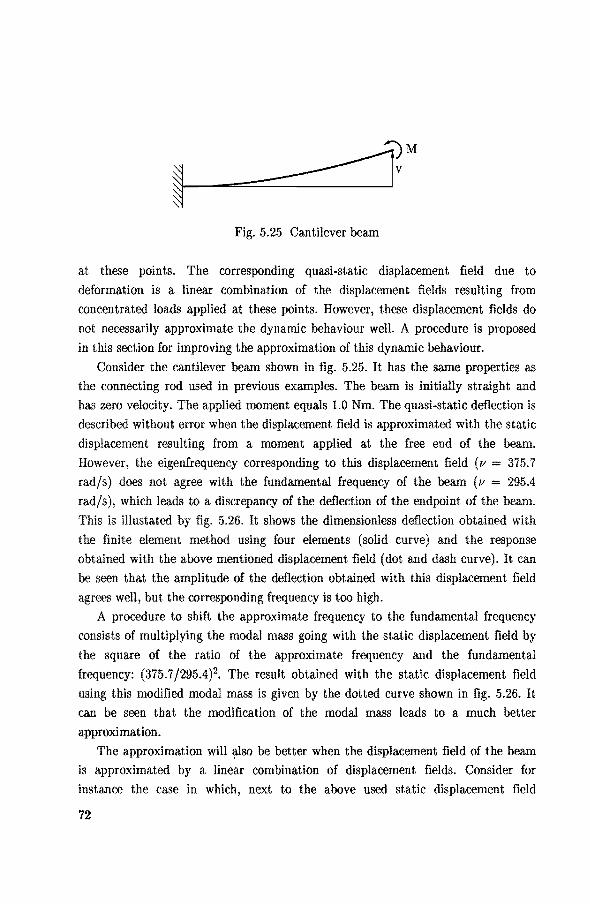
Fig. 5.25 Cantilever beam
at these points. The corresponding quasi-static displacement field due to
deformation is a linear combination of the displacement fields resulting from
concentrated loads applied at these points. However, these displacement fields do
not necessarily approximate the dynamic behaviour well. A procedure is proposed
in this section for improving the approximation of this dynamic behaviour.
Consider the cantilever beam shown in fig. 5.25. It has the same properties as
the connecting rod used in previous examples. The beam is initially straight and
has zero velocity. The applied moment equals 1.0 Nm. The quasi-static deflection is
described without error when the displacement field is approximated with the static
displacement resulting from a moment applied at the free end of the beam.
However, the eigenfrequency corresponding to this displacement field ( v = 375.7
radfs) does not agree with the fundamental frequency of the beam (v = 295.4
rad/s), which leads to a discrepancy of the deflection of the endpoint of the beam.
This is illustated by fig. 5.26. It shows the dimensionless defiection obtained with
the finite element metbod using four elements (solid curve) and the response
obtained with the above mentioned displacement field (dot and dash curve). It can
be seen that the amplitude of the deflection obtained with this displacement field
agrees well, but the corresponding frequency is too high.
A procedure to shift the approximate frequency to the fundamental frequency
consists of multiplying the modal mass going with the static displacement field by
the square of the ratio of the approximate frequency and the fundamental
frequency: (375.7/295.4)2• The result obtained with the static displacement field
using this modified modal mass is given by the dotted curve shown in fig. 5.26. It
can be seen that the modification of the modal mass leads to a much better
approximation.
The approximation will also be better when the displacement field of the beam
is approximated by a linear combination of displacement fields. Consicter for
instanee the case in which, next to the above used static displacement field
72

V/l
.02 fem solution
modal
.01 improved
.0
TIME (s)
Fig. 5.26 Influence of modifying mass matrix: one mode solution
resulting from a moment applied at the free end of the beam, the static
displacement resulting from a transverse force applied at the free end is used. Fig.
5.27 shows the response obtained with these two displacement fields (dot and dash
curve) and the response obtained with the finite element method using four
elements (solid curve). It can be seen that the approximation is now much better.
This is primarily due to the fact that the lowest eigenfrequency conesponding to
v/1
.02 fem solution
modal
.01 improved
.0
TIME (s)
Fig. 5.27 Influence of modifying mass matrix: two mode salution
73

the two displacement fields approximation is close to the fundamental frequency of
the beam.
The solution using two displacement fields can be improved with the above
described shifting procedure. The two displacement fields are orthogonalized before
the procedure is applied. This is accomplished by using them as base functions of
the space of eigenfunctions of the beam. The coefficients of the approximate
eigenfunctions relative to this base follow from the eigenvalue problem going with
the approximate equations of motion of the beam
(5.4)
where .Qs and K represent the modal mass matrix and the modal stiffness matrix,
respectively, going with the two static displacement fields. The two approximate
eigenfunctions which result from this analysis are used as base functions. From this
eigenvalue problem follows also an approximation of the two lowest eigenfrequen
cies of the beam. The modal masses going with the approximate eigenfunctions are
multiplied by the square of the ratio of the corresponding approximate eigenfre
quency and the corresponding exact eigenfrequency.
This procedure is applied to the above two static displacement fields. The
results obtained with the approximate eigenfunctions are identical to the result
obtained with the two static displacement fields, because they span the same vector
space of functions. The result obtained after modifying the modal masses is given
by the dotted curve in fig. 5.27. It can heseen that the modification of the modal
masses leads to a better approximation.
From the above it can he concluded that a more accurate discription of the
dynamic behaviour of a body can be obtained by shifting the approximate
eigenfrequencies of the body to its exact eigenfrequencies. However, more research
is needed to fully understand the proposed procedure and to justify its application.
It is feit that the procedure can also be used for improving the approximate solution
of the dynamic behaviour of a body which is part of a system of bodies. An
alternative application of the procedure is given in the next subsection.
5.6.2 Lowering of frequencies
The procedure that has been presented in the preceding subsection can also be used
to lower high frequencies in a model of a system of bodies. This may he desirabie
because high frequencies slow down the integration process. The modal synthesis
metbod is often used to reduce the number of degrees of freedom. The
74

eigenfrequendes conesponding to the retained displacement fields are generally low.
However, sometimes it may be beneficia! to retain displacement fields with which
correspond high frequencies. For example, an axial displacement field was included
in determining the nonlinear response of the planar slider-crank mechanism in
subsection 5.5.1 in order to determine the axial load in the connecting rod. The
frequency related to this displacement field is high as compared with the freqnency
going with the transverse deflection of the connecting rod, which slows down the
integration process. It is not important that the freqnency corresponding to the
axial displacement field is approximated correctly because the axial displacement
field is of minor importance for the deflection of the connecting rod; only its mean
value should be correct in order to obtain an accurate mean valne of the axialload.
The procedure presented in the preceding section is applied to the modal mass
conesponding to the axial displacement field of the connecting rod for the problem
considered in subsection 5.5.1. The modal mass is multiplied by respectively 10.0,
25.0, 50.0, and 100.0. The CPU times required for the analyses are respectively 0.5,
0.4, 0.3, and 0.2 times the CPU time required for the analysis using a consistent
modal mass. The deflection of the middle of the connecting rod is not influenced
when the modal mass is multiplied by 10.0 or 25.0; the response is slightly different
when the multiplier equals 50.0 or 100.0. This may be attributed to the fact that
the frequency is shifted too close to the eigenfrequency related to the transverse
deflection of the connecting rod.
It can be concluded that a high eigenfrequency can be lowered by multiplying
the modal mass by a factor > l.O. This factor should be such that the lowered
frequency does not approach the eigenfrequencies conesponding to relevant
displacement fields too close. The lowering of frequencies leads to CPU time
savings.
75
chapter 6
Concluding remarks
6.1 Conclusions
In this thesis, a mathematica! model is presented for determining the dynamic
behaviour of a deformable body which forms part of a system of bodies. For
descrihing the kinematics of the body, its displacement field is resolved into a
displacement field due to a rigid body motion and a displacement field due to
deformation. The displacement field due to deformation is chosen such that it does
not contain rigid body motions. Two kinds of conditions are considered to achieve
this, namely conditions for displacements of selected particles of the body and
conditions for mean displacements of the body. The latter conditions lead to
simpler equations of motion. The displacement field due to deformation is approxi
mated by a linear combination of a number of assumed displacement fields. Three
methods are considered for generating such displacement fields, namely the as
sumed-modes method, the finite element method, and the modal synthesis method.
The simplification of the equations of motion when the mean displacements
going witb tbe displacement field due to deformation are chosen equal to zero, leads
to a computation time r~uction of a few decades of per cents in the most
favourable case. For the systems investigated in this thesis the dynamic behaviour
is approximated better when the displacement field due to deformation is
approximated by assumed displacement fields witb mean displacements equal to
zero. Caution must be taken in preventing rigid body motions of tbe displacement
field due to deformation by prescrihing displacements of selected particles of the
body, since the solution of the dynamic behaviour may be incorrect.
Tbe assumed-modes metbod is only feasible for regularly shaped bodies. Tbe
finite element metbod and tbe modal syntbesis metbod can be used for bodies witb
arbitrary shape. Tbe finite element metbod leads often to a model with many
degrees of freedom. Tbe solution of sucb a model requires much computation time.
The modal synthesis metbod can tben be used to reduce tbe number of degrees of freedom sucb tbat tbe required computation time is cut down. The effectiveness of
tbe modal syntbesis metbod depends to a great extent on a proper cboice of tbe
assumed displacement fields. Such a cboice can generally be made in advance on tbe
basis of the load on the body. The lumped rnass approximation which is frequently
used in literature is feasible for determining time-independent mass coefficients
76
from displacement fields which have been determined with a standard finite
element program. One should bear in mind that a finer subdivision into elements
may be required than would be necessary for determining the displacement fields
sufficiently accurate.
A metbod is proposed to improve approximations for descrihing the dynamic
behaviour of a body for a specific set of assumed displacement fields. This method
has been used successfully for reducing the required computation time by lowering
irrelevant high frequencies.
6.2 Suggestions for further research
In section 2.5, the equations of motion of a body are written in terms of Euler
parameters and their first and second time derivatives in order to allow their
implementation in the computer program DADS. This leads to four equations that
describe the rotational motion of the body whereas three equations suffice.
Consequently, a constraint equation must be introduced which takes the dependen
cy of these equations into account. The equations of motion are simpler when they
are written in terms of the angular velocity vector and its first time derivative.
Further, time derivatives of eenstraint equations are more easily formulated in
terms of the angular velocity vector and its first time derivative. All this and the
results obtained by Nikraveshet aL (1985) indicate that a computer program based
on the equations of motion in terms of the angular velocity vector and its first time
derivative will be more efficient. This may be a fruitful topic for further research.
Computer programs for the analysis of the dynamic behaviour of multibody
systems are based on either the global description or the relative description. The
description given by Haug and McCullough (1986) may be regarded as an irnpulse
to arrive at a program which is based on a synthesis of the global description and
the relat.ive description. They derived the equations of motion of recurring
subsystems in terrus of variables that describe the relative motion of the
interconnected boclies in the subsystem and implemented them into the multibody
program DADS, which is based on the global description. This approach could be
extended such that it is not necessary to derive the equations of motion of a specific
subsystem in symbolic form and to implement them into a multibody program.
This requires the addition of a module that automatically evaluates the equat.ions
of motion of any subsystem using the relative description. Perhaps it is even
possible to give guidelines on which description is most efficient for a specific
system. These can then be used by the program to select the most efficient
description automatically. 77
The constraint equations for kinematic connections which are implemented in
computer programs that are based on the global description are generally written in
terms of the kinematic variables of the interconnected bodies. These equations
cannot be solved explicitly for specific variables. However, they can be solved
explicitly when variables that describe the relative motion of the interconnected
bodies are introduced such as is done in the relative description. This can be used in
solving the equations of motion of multibody systems with a tree structure, by
circumventing the need to solve the constraint equations iteratively and to
partition variables into dependentand independent variables numerically. Actually,
such a description leads to the relative description within a program based on the
global description. It can be implemented without difficulty in a multibody
program such as DADS, since some kinematic connections are already described
using the variables that describe the relative motion of the interconnected bodies.
Therefore, research should be devoted to a solution procedure that takes advantage
of the fact that the constraint equations can be solved explicitly.
A good choice of assumed displacement fields for a specific body can generally
be made on the basis of the load on the body. This presents no difficulties when the
type of load does not change much. However, the selection of assumed displacement
fields is not straightforward when the type of load changes considerably. This may
be the case when the point of application of the load changes, such as occurs for a
body which is interconnected by a translational joint to another body. The best
choice for a set of assumed displacement fields depends on the instantaneous
location of the point of contact. Such a dependency cannot be accounted for with
the description given in this thesis because the assumed displacement fields are
taken invariable. Wang and Wei (1987) presented a mathematica! modelfora beam
which takes a change of assumed displacement fields into account. They approxi
mated the displacement field of the beam with instantaneous eigenfunctions.
However, the instantaneous eigenfrequencies go to infinity when the point of
contact approaches the end of the beam which slows down the integration process.
Another option might be to waive the wish to use an instantaneous good set of
assumed displacement fields and use displacement fields that do not change. This
approach has been foliowed by Hwang and Haug (1987). A failure of this approach
is that the displacement fields due to deformation of the body on both sides of the
translational joint are coupled, which may lead to incorrect results. Further, it may
be necessary to include a relatively large number of assumed displacement fields
which leads to long computation times. The selection of assumed displacement
fields for bodies with the above discribed loading requires further research.
78
References
Agrawal, 0. P., and Shabana, A. A., 1985, "Dynamic Analysis of Multibody
Systems Using Component Modes," Computers & Structures, Vol. 21, pp.
1303-1312.
Arnold, F. R., 1962, "Algebra," in Handbook of Engineering Mechanics (Flügge,
W., Ed.), McGraw-Hill, New York, chapter 1.
Ashley, H., 1967, "Observations on the Dynamic Behavior of Large Flexîble Bodies
in Orbit," AJAA J., Vol. 5, pp. 460-469.
Bakr, E. M., and Shabana, A. A., 1986, "Geometrically Nonlinear Analysis of
Multibody Systerns," Computers & Structures, Vol. 23, pp. 739-751.
Baumgarte, J., 1972, "Stabilization of Constraints and Integrals of Motion in
Dynamical systems," Computer Methods in Applied Jvfechanics and Engineering,
Vol. 1 pp. 1-16.
Baumgarte, J., 1978, "Stabilisierung von Bindungen in Lagrangeschen
Formalismus," ZAMM, Vol. 58, pp. T360-T361.
CAD SI, 1988, DADS User's Manual, Rev. /i. 0, Computer Aided Design Software,
Oakdale, IA.
Casey, J., 1983, "A Treatment of Rigid Body Dynamics," J. of Applied Mechanics,
Vol. 50, pp. 905-907; 1984, Vol. 51, p. 227.
Chadwick, P., 1976, Continuurn Mechanics, George Allen & Unwin, London.
Chang, C. 0., and Nikravesh, P. E., 19815, "An Adaptive Gonstraint Vialation
Stabilization Metbod for Dynarnic Analysis of Mechanica! Systems," J. of
Mechanisms, Transmissions, and Automation in Design, Vol. 107, pp. 488-492.
Changizi, K., Khulief, Y. A., and Shabana, A. A., 1986, "Transient Analysis of
Flexible Multi-body Systems. Part II: Application to Aircraft Landing," Computer
Methods in Applied Mechanics and Engineering, Vol. 54, pp. 93-110.
Craig, R. R., 1981, Structural Dynamics: An Introduetion to Computer Methods,
Wiley, New York.
Erdman, A. G., and Sandor, G. N., 1972, "Kineto-Elastodynarnics-A Review of the
State of the Art and Trends," Mechanism and Machine Theory, VoL 7, pp. 19-33.
79
Gurtin, M. E., 1981, An Introduetion to Continuurn Mechanics, Academie Press,
New York.
Haug, E. J., and McCullough, M. K., 1986, "A Variational-Vector Calculus
Approach to Machine Dynamics," J. of Mechanisms, Transmissions, and Automation in Design, Vol. 108, pp. 25-30.
Haug, E. J., Wu, S. C., a.nd Kim, S. S., 1986, "Dynamics of Flexible Machines, A
Variational Approach," in Dynamics of Multibody Systems (Bianchi, G., and
Schiehlen, W., Eds.), Springer-Verlag, Berlin, pp. 55-67.
Huston, R. L., a.nd Passerello, C., 1979, "On Multi-Rigid-Body System Dynamics,"
Gomputers & Structures, Vol. 10, pp. 439-446.
Hwang, R.-S., a.nd Haug, E. J., 1987, Translational Joint Formulations in Flexible Machine Dynamics, Technica} Report 86-13, Center for Computer Aided Design
a.nd College of Engineering, The University of lowa, lowa City, Iowa.
Jonker, J. B., 1988, A Finite Element Dynamic Analysis of Flexible Spatial Mechanisms and Manipulators, Ph.D. thesis, Delft University of Technology, Delft.
Ka.ne, T. R., 1968, Dynamics, Holt, Rinehart, and Winston, New York.
Kane, T. R., and Levinson, D. A., 1983, 11Multibody Dynamics," J. of Applied Mechanics, Vol. 50, pp. 1071-1078.
Kline, K. A., 1986, "Dynamic Analysis Using A Reduced Basis of Exact Modes and
Ritz Vectors," A/AA J., Vol. 24, pp. 2022-2029.
Koplik, J., and Leu, M. C., 1986, "Computer Generation of Robot Dynamica
Equations and the Related Issues," J. of Robotic Systems, Vol. 3, pp. 303-319.
Koppens, W. P., Sauren, A. A. H. J., Veldpaus, F. E., and Campen, D. H. van,
1988, "The Dynamica of a Deformable Body Experiencing Large Displacements," J.
of Applied Mechanics, Vol. 55, pp. 676-680.
Li, D., and Likins, P. W., 1987, Dynamica of a Multibody System with Relative
Translation on Curved, Flexible Tracks," J. of Guidance, Control and Dynamics, Vol. 10, pp. 299-306.
Lilov, L.K., and Chirikov, V. A., 1982, "On the Dynamics Equations of Systems of
Interconnected Bodies," J. of Applied Mathernaties and Mechanics, Vol. 45, pp.
383-390.
80

Lilov, L., and Wittenburg, J., 1986, "Dynamics of Chains of Rigid Bodies and
Elastic Rods with Revolute and Prismatic Joints," in Dynamics of Afultibody
8ystems (Bianchi, G., and Schiehlen, W., Eds.), Springer-Verlag, Berlin, pp.
141-152.
Malvern, L. E., 1969, Introduetion to the Mechanics of a Continuous Medium,
Prentice-Hall, Englewood Cliffs, N.J.
McCullough, M. K., and Haug, E. J., 1986, "Dynamics of High Mobility Track
Vehicles," J. of Mechanisms, Transmissions, and Automation in Design, VoL 108,
pp. 189-196.
McDonough, T. B., 1976, "Formulation of the Global Equations of Motion of a
Deformable body," AIAA J., VoL 14, pp. 656-660.
Mclnnis, B. C., and Liu, C.-F. K., 1986, "Kinematics and Dynamics in Robotics: A
Tutorial Based U pon Classica! Conceptsof Vectorial Mechanics," IEEE J. Robotics
and Automation, VoL RA-2, pp. 181-187.
Meirovitch, L., 1970, Methods of Analytica[ Dynamics, McGraw-Hill, New York.
Newell, H. E., 1962, "Vector analysis," in Handbook of Engineering Mechanics
(Flügge, W., Ed.), McGraw-Hill, New York, chapter 6.
Nikravesh, P. Kwon, 0. K., and Wehage, R. A., 1985, "Euler Parameters in
Computational Kinematics and Dynamics. Part 2," J. of Mechanisms,
Transmissions, and Automation in Design, VoL 107, pp. 366-369.
Orlandea, N., Chace, M. A., and Calahan, D. J. , 1977a, "A Sparsity-Oriented
Approach to the Dynamic Analysis and Design of Mechanica! Systems-Part 1," J.
of Engineering for Industry, VoL 99, pp. 773-779.
Orlandea, N., Chace, M. A., and Calahan, D. A., 1977b, "A Sparsity-Oriented
Approach to the Dynamic Analysis and Design of Mechanica! Systems-Part 2," J.
of Engineering for Industry, VoL 99, pp. 780-784.
Park, T., and Haug, E. J., 1985, Numerical 1\lethods jor Mixed Differential
Algebraic Equations in Kinematics and Dynamics, Technica! Report 85-23, Center
for Computer Aided Design and College of Engineering, The University of Iowa,
Iowa City, Iowa.
Park, T. W., and Haug, E. J., 1986, "A Hybrid Numerical Integration Metbod for
Machine Dynamic Simulation," J. of Mechanisms, Transmissions, and Automation
in Design, Vol. 108, pp. 211-216.
81

Przemieniecki, J. S., 1968, Theory of Matrix Structural Analysis, McGraw-Hill,
New York.
Rao, S. S., 1982, The Finite Element Method in Engineering, Pergamon Press,
Oxford.
Rosenberg, R. M., 1977, Analytica[ Dynamics of Discrete Systems, Plenum Press,
New York and London.
Samin, J.-C., and Willems, P. Y., 1986, "Multibody Formalism Applied to
Non-Conventional Railway Systems," in Dynamics of Multibody Systems (Bianchi,
G., and Schiehlen, W., Eds.), Springer-Verlag, Berlin, pp. 237-248.
Schiehlen, W., 1981, "Nichtlineare Bewegungsgleichungen Grofier Mehrkörper
systeme," ZAMM, Vol. 61, pp. 413-419.
Schiehlen, W., 1984, "Dynamics of Complex Multibody Systems," SM Archives,
Vol. 9, pp. 159-195.
Schiehlen, W., 1986, Technische Dynamik, B. G. Teubner, Stuttgart.
Shabana, A. A., 1986, "Transient Analysis of Flexible Multi-body Systems. Part 1:
Dynamics of Flexible Bodies," Computer Methods in Applied Mechanics and
Engineering, Vol. 54, pp. 75-91.
Shampine, L. F., and Gordon, M. K., 1975, Computer Solution of Ordinary
Differential Equations: The Initial Value Problem, W. J. Freeman, San Francisco.
Singh, R. P., VanderVoort, R. J., and Likins, P.W., 1985, "Dynamics of Flexible
Bodies in Tree Topology-A Computer Oriented Approach," J. of Guidance,
Control and Dynamics, Vol. 8, pp. 584-590.
Singh, R., VanderVoort, R., and Likins, P., 1986, "lnteractive Design for Flexible
Multibody Control," in Dynamics of Multibody Systems (Bianchi, G., and
Schiehlen, W., Eds.), Springer-Verlag, Berlin, pp. 275-286.
Simo, J. C., and Vu-Quoc, 1., 1986, "On the Dynamics of Flexible Beams Under
Large Overall Motions-The Plane Case: Part I," J. of Applied Mechanics, Vol. 53,
pp. 849-854.
Sol, E. J., 1983, Kinematics and Dynamics of Multibody Systems, Ph.D. thesis,
Eindhoven University of Technology, Eindhoven.
82

Song, J. 0., and Haug, E. J., 1980, "Dynamic Analysis of Planar Flexible
Mechanisms," Computer Methods in Applied Mechanies and Engineering, Vol. 24,
pp. 359-381.
Sunada, W., and Dubowsky, S., 1981, "The application of Finite Element Methods
to the Dynamic Analysis of Flexible Spatial and Co-Planar Linkage Systems," J. of
Mechanica/ Design, Vol. 103, pp. 643-651.
Sunada, W. H., and Dubowsky, S., 1983, "On the Dynamic Analysis and Behavior
of Industrial Robotic Manipulators With Elastic Members," J. of Mechanisms,
Transmissions, and Automation in Design, Vol. 105, pp.42-50.
Sung, C. K., Thompson, B. S., Xing, T. M., and Wang, C. H., 1986, "An
Experimental Study on the Nonlinear Elastodynamic Response of Linkage
Mechanisms," Mechanism and Machine Theory, Vol. 21, pp. 121-133.
Thornpson, B. S., and Sung, C. K., 1984, "A Variational Formulation for the
Nonlinear Finite Element Analysis of Flexible Linkages: Theory, Irnplernentation,
and Experirnental Results," J. of Mechanisms, Transmissions, and Automation in
Design, Vol. 106, pp. 482-488.
Turcic, D. A., and Midha, A., 1984a, "Generalized Equations of Motion for the
Dynamic Analysis of Elastic Mechanism Systerns," J. of Dynamic Systems,
Measurement, and Control, Vol. 106, pp. 243-248.
Turcic, D. A., and Midha, A., 1984b, "Dynamic Analysis of Elastic Mechanism
Systems. Part I: Applications," J. of Dynamic Systems, Measurernent, and Control,
Vol. 106, pp. 249-254.
Wang, P. K. C., and Wei, Jin-Duo, 1987, "Vibrations in a Moving Flexible Robot
Arm," J. ofSound and Vibration, Vol. 116, pp. 149-160.
Weeën, F. van der, 1985, Eindige Elementen voor Kineto-Elastodynamische Analyse
van Mechanische Systemen, Ph.D. thesis, Rijksuniversiteit Gent, Gent.
Wehage, R. A., and Haug, E. J., 1982, "Generalized Coordinate Partitioning for
Dirneusion Rednetion in Analysis of Constrained Dynamic Systerns," J. of
Mechanica/ Design, Vol. 104, pp. 247-255.
Werff, K. van der, and Jonker, J. B., 1984, "Dynarnics of Flexible Mechanisms," in
Computer Aided Analysis and Optirnization of Mechanica/ Systern Dynamics (Haug,
E. J., Ed.), Springer-Verlag, Berlin Heidelberg, pp. 381-400.
83

Wittenburg, J., 1977, Dynamics of Systems of Rigid Bodies, B. G. Teubner,
Stuttgart.
Wittenburg, J., 1987, "Multibody Dynamics. A Rapidly Developing Field of
Applied Mechanics," Meccanica, Vol. 22, pp. 139-143.
Yoo, W. S., and Haug, E. J., 1986a, "Dynamics of Flexible Mechanical Systems
Using Vibration and Static Correction Modes," J. of Mechanisms, Transmissions, and Automation in Design, Vol. 108, pp. 315-322.
Yoo, W. S., and Haug, E. J., 1986b, "Dynamics of Articulated Structures-Part I:
Theory," J. ofStructural Mechanics, Vol. 14, pp. 105-126.
Yoo, W. S., and Haug, E. J., 1986c, "Dynamics of Articulated Structures-Part II:
Computer Implementation and Applications," J. of Structural Mechanics, Vol. 14,
pp. 177-189.
Zienkiewicz, 0. C., 1977, The Finite Element Method, McGraw-Hill, London.
84
appendix A
Mathematica! notation
A.1 Matrices
An m x n matrix is defined as a set of objects arranged in m rows and n colunms.
The objects may be for instanee scalars, vectors, tensors or matrices. Matrices will
be designated by an underscore; for legibility, column matrices will be designated
by a wavy underscore. Matrices are sametimes denoted by the elernents enclosed in
brackets. A typieal element of a matrix is denoted by the matrix syrnbol sub
scripted by its row and column nurnber. The column number 1 for elements of a
column matrix wil! be ornitted. The name-giving of special rnatrices and operations
on rnatrices agree with the norrnally used definitions (cf. e.g. Arnold; 1962).
Multiplication of a matrix with another object is evaluated by the common
multiplication rule of matrix algebra with the understanding that the operatien on
the elements of the matrix and the other object is governed by the operator
between the matrix and the object. For example, when the elements of the matrix
and the object are vector quantities, then a · indicates that the resulting matrix
elements are scalars obtained from scalar multiplication of the elements of the
matrix and the objects.
The skew-symmetric 3 x 3 matrix that corresponds to a 3 x 1 column matrix ~
in accordance with the definition
(A.l)
is given a wavy superscript in order to discrirninate it from other matrices. The
elementsof IJ. may be scalars, veetors or tensors.
A.2 Veetors and tensors
Veetors are entities defined in a Euclidean vector space that possess both mag
nitude and direction. They are often visualized by an arrow that is pointing in the
direction associated with the vector and that has a length equal to the magnitude of
the vector. Veetors will be designated by letters with an arrow as superscript.
85

Veetors as used in this thesis have the usual properties (cf. e.g. Newell, 1962).
The scalar product of an arbitrary pair of veetors a and b is denoted by a· b. It is a scalar with magnitude equal to the product of the magnitude of the two veetors
and the eosine of the angle between the vectors.
The vector product of an arbitrary pair of veetors a and b is denoted by a x b. It is a vector perpendicular to the two veetors with magnitude equal to the product of
the magnitude of the two veetors and the sine of the angle between the two vectors; ... ~ ... ...
the sense of the vector is such that a, b and a x b make a right-handed system.
The tensor product of an arbitrary pair of veetors a and b is denoted by ab. lt is
a linear vector operator, called dyad, that can be used to form for instanee the
scalar product with an arbitrary vector ê yielding a vector such that
...... -t ....... (ab)·c = (b·c)a, (A.2)
.. ...... .. ..... c·(ab) = (a·c)b. (A.3)
A secoud order tensor is a linear combination of dyads. In this thesis only
secoud order tensors are used. They are identified by boldface letters. Such as for
dyads, secoud order tensors can be used to form scalar products with an arbitrary
vector yielding a vector. This vector follows from the definitions of the scalar
product of a dyad and a vector.
The product of two second order tensors, A and B, is denoted by A· B. It is a
second order tensor such tbat
... ... ... ... a·(A·B)·b = (a·A)·(B·b) (A.4)
for all veetors a and b. .. .. .. The trace of a tensor A, denoted by tr( A), is a scalar sucb that for a· (b x c) f. 0
(A·a)·(b x ê) + a·{(A·b) x ê} + a·{b x (A·ê)} = tr(A) a·(b x ê) (A.s)
.. .. .. This scalar does not depend on a, b or c.
The scalar product of two secoud order tensors, A and B, is denoted by A:B. It
is a scalar such that
A:B = tr(A·B). (A.6)
The conjugale tensor of an arbitrary tensor A, denoted by Ac, is a secoud order
tensor sucb that
86
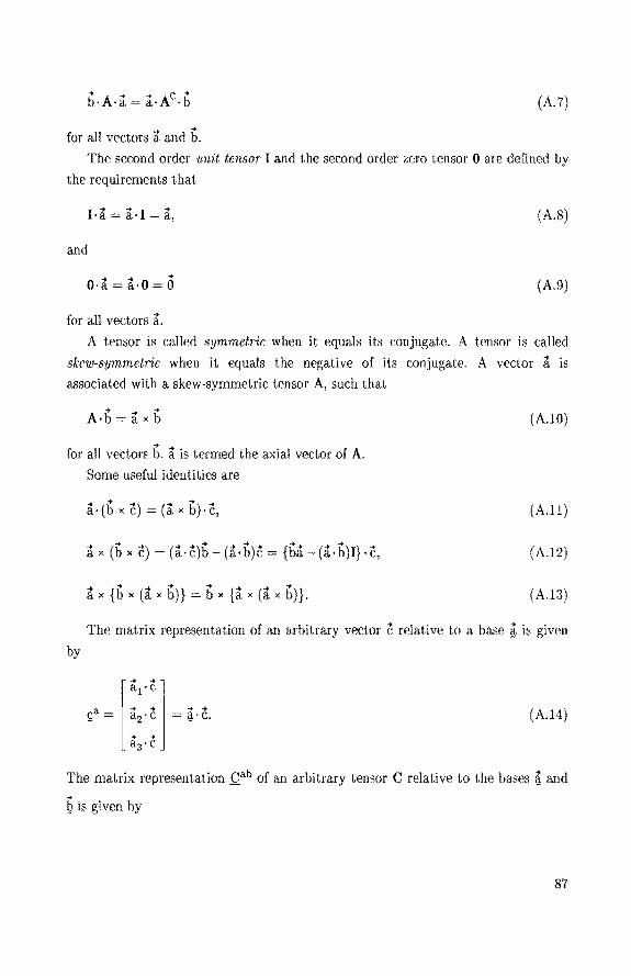
(A.7)
for all veetors a and b. The second order unit tensor I and the second order zero tensor 0 are defined by
the requirements that
I·a = a·I =a, (A.S)
and
... .. .. O·a=a·O=O (A.9)
for all veetors a. A tensor is called symmetrie when it equals its conjugate. A tensor is called
skew-symmetric when it equals the negative of its conjugate. A vector a is associated with a skew-symmetric tensor A, such that
(A.lO)
for all veetors b. a is termed the axial vector of A.
Some useful identities are
.. .. "') .. ~ ... a·(b x c =(a x b)·c, (A.ll)
(A.12)
a x {b x (a x b)} = b x {a x (a x b)}. (A.l3)
The matrix representation of an arbitrary vector c relative to a base ~ is given
by
[. . a1• c
ça ... ... ... ... (A.l4) a2·c !J.·C.
... ... a3 ·c
The matrix representation ç_ab of an arbitrary tensor C relative to the bases (! and
Sis given by
87

-+ -+T = !!-·C·g. (A.15)
In this thesis the matrix representation of all veetors and tensors are relative to the
same base, namely an orthorrormal right-handed inertial base ~. Consequently there
is no need to specify the base that is used for determining the matrix representa
tion.
88

appendix B
Description of rotational motion in terniS of Euler parameters
From Euler's theorem, a rotation about a fixed point may be conceived as the
result of a rotation about a unique axis passing through that point (Wittenburg,
1977). Let the direction of that axis be defined by the unit vector e and the angle of
rotation by X· Then from fig. B.l the position vector of an arbitrary material point
P in its reference configuration, x, and the position vector of P after a rotation
about an axis passing through an inertial point 0, t, are related by the equation
t x+ (1- cosx)w + sinx v, (B.l)
where v is perpendicular to the plane spanned by x and e, a.nd ,-v is perpendicular to
e and v; the length of both v and w equal the radius of the circle traversed by P due
to the rotation. From this v and w can be written in termsof e and x. This yields
-> -> ... v ex x,
-+ ... -+ ... (.. ...) w=exv=ex exx.
Fig. B.l Rotation about e
~ e
(B.2)
(B.3)
89

Substitution of (2) and (3) into (1) yields
.. .. .. (.. ..) .. .. r = x + 2q x q x x + 2q0q x x, (B.4)
where
q0 cos(x/2), (B.5)
q ê sin(x/2). (B.6)
~ and the components of q relative to an arbitrary orthonormal inertial base ~ are
called Euler parameters. Since ê is a unit vector, the Euler parameters are related
by
2 .... qo+q·q=l. (B.7)
For any vector a and q there exists a skew-symmetric tensor R such that
(B.8)
From this equation it can be shown that R is related to the components of q relative to the base ~ by
(B.9)
Substitution of {8) into (4) yields
(B.lO)
Oomparing this expression with the expression for a rigid body rotation
(B.ll)
reveals that
Q = I+ 2R· R + 2q0R. (B.l2)
Substitution of (9) into (12), using (7), yields for the components of Q relative to ~
90

[
qÖ + qf - q~ q5
2( qlq2 + q0q3)
2(ql~- q0q2)
2( qlq2 - q0q3) 2( qlq3 + q0q2)
qÖ - q1 + q~ q~ 2(q2q3- qûql) (B.13)
2( q2q3 + QoQ 1) qfi - qÎ q~ + q§
The angular velocity vector wis the axial vector of Qc · Q. Aftersome algebrak
manipulation, using (7) and its first time derivative, the following result can be
obtained
... 2 ... TG. W= § _g,
where
and
[ -ql Qo Q3 -q2]
= -qz -q3 Qo ql ·
-q3 q2 -qt Qo
Similarly, the virtual angular rotation equals
lt may be verified that
Qg= Q.
Consequently the expression for the angular acceleration becomes
(B.14)
(B.15)
(B.l6)
(B.l7)
(B.18)
(B.19)
The component form of (14) relative to ~ is obtained from scalar premultiplication
of (14) by ~. This yields
(B.20)
where '!!is the column matrix of the componentsof w relative to ~. Solving (20) and
the first time derivative of (7) for g yields
(B.21)
91
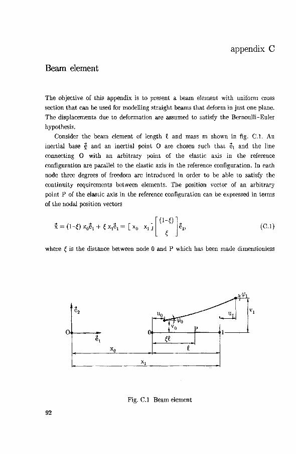
appendix C
Beam element
The objective of this appendix is to present a beam element with uniform cross
section that can be used for modeHing straight beams that deform in just one plane.
The displacements due to deformation are assumed to satisfy the Bernoulli-Euler
hypothesis.
Consider the beam element of length t and mass m shown in fig. C.l. An
inertial base ~ and an inertial point 0 are chosen such that el and the line
connecting 0 with an arbitrary point of the elastic axis in the reference
configuration are parallel to the elastic axis in the reference configuration. In each
node three degrees of freedom are introduced in order to be able to satisfy the
continuity requirements between elements. The position vector of an arbitrary
point P of the elastic axis in the reference configuration can be expressed in terms
of the noclal position veetors
(C.l)
where Ç is the distance between node 0 and P which has been made dimensionless
Fig. C.l Beam element
92

with t. The displacements between the nodes are interpolated with the usual
Hermite polynomials
.. T .. u(Ç,t) = eQ: (t) e<P(Ç), (C.2)
where
(C.3)
e~( Ç) [(1-Ç)el (1-3ç2+2Ç3)e2 .€.( Ç-2Ç2+Ç3)ê2
{e1 (3e-2çJ)e2 t( -e+Ç3)ê2 ] r. (C.4)
Using this approximation of the displacement field due to deformation, the
time-independent inert ia coefficients (2.34 )-(2.41) become for this beam element
(C.5)
(C.6)
(C.7)
(C.8)
(C.9)
(C.lO)
(C.ll)
(C.l2)
where
93

2 1
0 0
0 0 Mt (m/6) 1 2 '
(C.l3)
0 0
0 0
0 0
21 9
3t 2t M2 = (m/60) 0 0 '
(C.l4)
9 21
-2t -3t
2 0 0 1 0 0
0 0 0 0 0 0
0 0 0 0 0 0 Ms = (m/6) 1 0 0 2 0 0 '
(C.15)
0 0 0 0 0 0
0 0 0 0 0 0
0 0 0 0 0 0
0 156 22t 0 54 -13t
0 22t 4t2 0 13t -3t2
~ (m/420) 0 0 0 0 0 0 (C.16)
0 54 13t 0 156 -22t
0 -13t -3t2 0 -22t 4t2
0 0 0 0 0 0
21 0 0 9 0 0
3t 0 0 2t 0 0 ~ = (m/60) 0 0 0 0 0 0 (C.17)
9 0 0 21 0 0
-2t 0 0 -3t 0 0
The expression for the strain energy of a beam, using linearized strain-
displacement relations, is given by
94
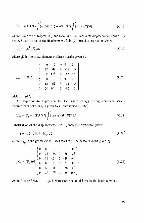
1 1
U1 !(EA/t) J (àu/iJÇ)2dÇ + !(EI/t3) J (0Zv/iJÇ2?dÇ, (C.l8)
0 0
where u and v are respectively the a:x:ial and the transverse displacement field of the
beam. Substitution of the displacement field (2) into this expression yields
UI .l T K ze9' e- e9', (C.l9)
where is the usual element stiffness matrix given by
7 0 0 -7 0 0
0 12 6t 0 -12 6t
0 6t 4t2 0 -6( 2t2
(EI/t 3) -Î 0 0 7 0 0 (C.20)
0 -12 -6t 0 12 -6t
0 6t 2t 2 0 -6( 4t 2
with ~/ At 2/T. An approximate expression for the strain energy, using nonlinear strain
displacement relations, is given by (Przemieniecki, 1968)
1
Uni U1 + !(EA/t2) J (àu/oÇ)(IN/iJÇ)2dÇ. (C.21)
0
Substitution of the displacement field (2) into this expression yields
(C.22)
where J{G is the geometrie stiffness matrix of the beam element given by
0 0 0 0 0 0
0 36 3( 0 -36 3(
0 3( 4t2 0 -3( -(2
J{G (F /30t) 0 0 0 0 0 0 (C.23)
0 -36 -3t 0 36 -3t 0 3( -(2 0 -3t 4(2
where F = (EA/t)/(u1 - u0). F represents the axial force in the beam element.
95
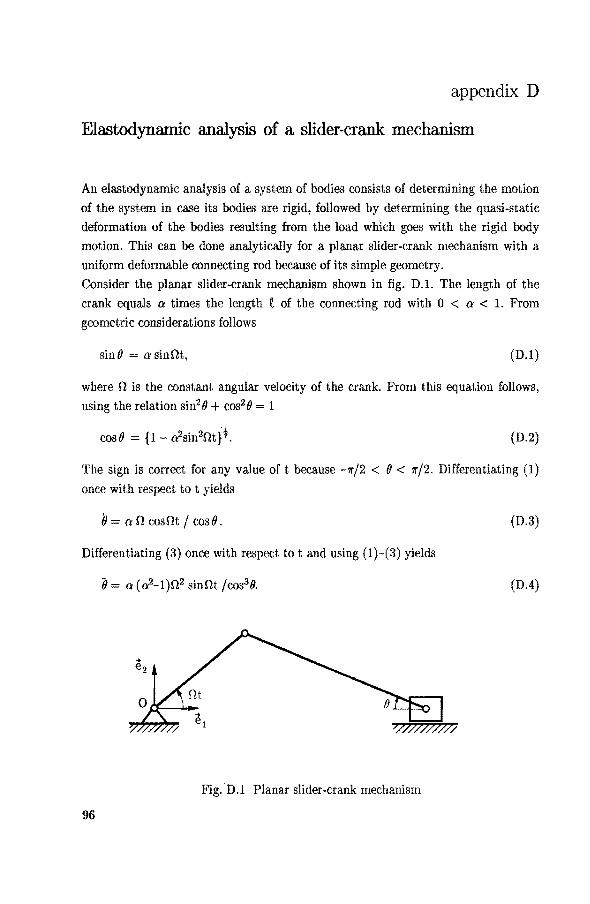
appendix D
Elastodynamic rumlysis of a slider·crank mechanism
An elastodynamic analysis of a system of bodies consistsof determining the motion
of the system in case its bodies are rigid, followed by determining the quasi-static
deformation of the bodies resulting from the load which goes with the rigid body
motion. This can be done analytically for a planar slider-crank mechanism with a
uniform deformable connecting rod because of its simple geometry.
Consider the planar slider-crank mechanism shown in fig. D.I. The length of the
crank equals a times the length t of the connecting rod with 0 < a < 1. From
geometrie considerations follows
sin 0 = a sinnt, (D.l)
where n is the constant angular velocity of the crank. From this equation follows,
using the relation sin2 0 + cos2 0 = 1
(D.2)
The sign is correct for any value of t because -7r/2 < 0 < 1rj2. Differentiating (1)
once with respect to t yields
ó = a n cosnt f cos 0 . (D.3)
Differentiating (3) once with respect tot and using (1 )-(3) yields
(D.4)
Fig. D.l Planar slider-crank mechanism
96
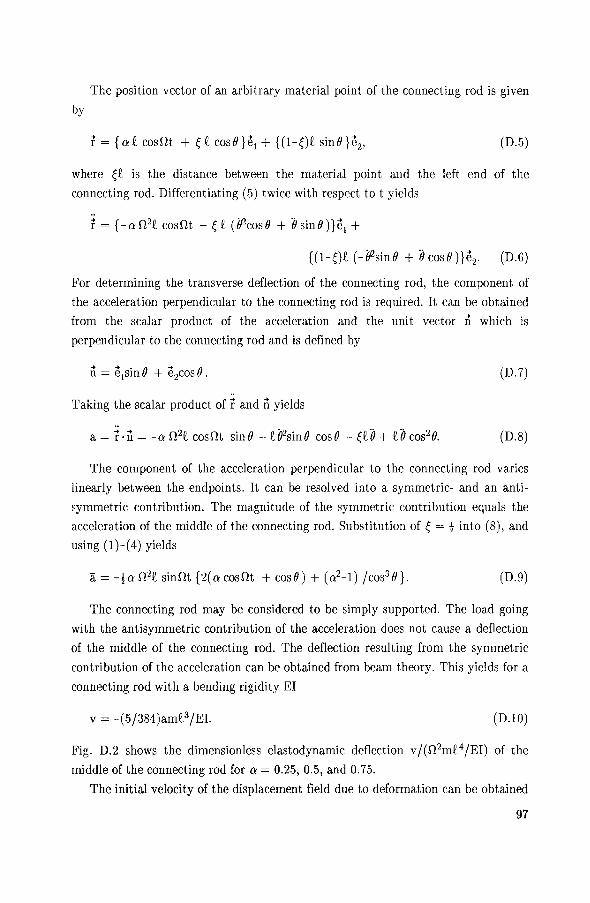
The position vector of an arbitrary material point of the connecting rod is given
by
r ={at cosnt + Ç t cosO}e1 + {(1-Ç)t sinO}e2, (D.5)
where Çt is the distance between the material point and the left end of the
connecting rod. Differentiating (5) twice with respect tot yields
{(1-Ç)t (-è2sin0 + ÖcosO)}ê2. (D.6)
For determining the transverse deflection of the connecting rod, the component of
the acceleration perpendicular to the connecting rod is required. It can be obtained
from the scalar product of the acceleration and the unit vector n which is
perpendicular to the connecting rod and is defined by
(D.7)
Taking the scalar product of r and n yields
a= r ·n =-a n 2t cosnt sinO- tè2sin0 cosO - Çtë + të cos20. (D.S)
The component of the acceleration perpendicular to the connecting rod varies
linearly between the endpoints. It can be resolved into a symmetrie- and an anti
symmetrie contribution. The magnitude of the symmetrie contribution equals the
acceleration of the middle of the connecting rod. Substitution of Ç = t into (8), and
using (1)-(4) yields
a= -tan2t sinnt {2(acosnt + cosO) + (a2-1) jcos3 0}. (D.9)
The connecting rod may be considered to be simply supported. The load going
with the antisymmetrie contribution of the acceleration does not cause a deflection
of the middle of the connecting rod. The deflection resulting from the symmetrie
contri bution of the acceleration can be obtained from beam theory. This yields for a
connecting rod with a bending rigidity EI
v = -(5/384)amt3/EI. (D.10)
Fig. D.2 shows the dimensionless elastodynamic deflection vj(n2mt4/EI) of the
middle of the connecting rod fora= 0.25, 0.5, and 0.75.
The initia! velocity of the displacement field due to deformation can be obtained
97

----- a 0.25 .005
--·-- a=0.50
-.005
.0 1t 21t CRANK ANGLE (rad)
Fig. D.l Elastodynamic deflection of the middle of the connecting rod
from differentiation of (10) once with respect to t and substituting t = 0 s. This
yields
(D.ll)
where ä0 is the time derivative of the mean acceleration for t = 0 s, given by
(D.l2)
98

Samenvatting
In dit proefschrift wordt een wiskundige beschrijving gegeven van het dynamisch
gedrag van stelsels van onderling verbonden vervormbare lichamen.
Het verplaatsingsveld van een lichaam wordt opgesplitst in een verplaatsings
veld als gevolg van een beweging als star lichaam en een verplaatsingsveld als
gevolg van vervorming. Om deze opsplitsing eenduidig te maken, wordt van het
verplaatsingsveld als gevolg van vervorming geëist dat het geen beweging als star
lichaam representeert. Dit kan worden bereikt door Of verplaatsingen als gevolg van
vervorming van een aantal materiële punten of gemiddelde verplaatsingen als
gevolg van vervorming, voor te schrijven.
Uitgaande van de bewegingsvergelijkingen voor een infinitesimaal volume
element van het lichaam wordt een variationele formulering voor de bewegingsver
gelijkingen van het vrijgemaakte lichaam afgeleid. Deze vergelijkingen zijn
eenvoudiger indien de gPmiddelde verplaatsingen als gevolg van vervorming gelijk
aan nul zijn. Een benaderingsoplossing voor de bewegingsvergelijkingen wordt
verkregen door het verplaatsingsveld als gevolg van vervorming te benaderen met
een lineaire combinatie van een aantal aangenomen verplaatsingsvelden. Drie
methoden voor het genereren van dergelijke verplaatsingsvelden worden beschreven,
namelijk de "assumed-modes" methode, de eindige elementen methode en de
"modal synthesis" methode.
V oor het opstellen van de bewegingsvergelijkingen van het lichaam zoals het
voorkomt in een stelsel van lichamen, moet rekening worden gehouden met verbin
dingen met andere lichamen. Energetische en actieve verbindingen kunnen in
rekening worden gebracht door de krachten die zij veroorzaken toe te voegen aan de
krachten op het vrijgemaakte lichaam. Kinematische verbindingen beperken de
bewegingsvrijheid van de onderling verbonden lichamen. Dit kan in rekening
worden gebracht met constraintvergelijkingen, waarmee de variabelen die de
kinematica van het stelsel van lichamen beschrijven, kunnen worden onderverdeeld
in afhankelijke en onafhankelijke variabelen. Het is handig om bij het formuleren
van de constraintvergelijkingen, variabelen te introduceren die de relatieve bewe
ging van de verbonden lichamen ten opzichte van elkaar beschrijven.
Het eenvoudiger zijn van de bewegingsvergelijkingen wanneer de gemiddelde
verplaatsingen als gevolg van vervorming gelijk aan nul zijn gekozen, leidt in het
gunstigste geval tot een rekentijdbesparing van enkele tientallen proeen ten. Van
99
de in dit proefschrift onderzochte systemen wordt het dynamisch gedrag beter
benaderd indien verplaatsingsvelden als gevolg van vervorming worden benaderd
met aangenomen verplaatsingavelden waarvan de gemiddelde verplaatsingen als
gevolg van vervorming gelijk aan nul zijn. Het voorkomen van bewegingen als star
lichaam in .het verplaatsingaveld als gevolg van vervorming door het voorschrijven
van componenten van verplaatsingen van materiële punten moet behoedzaam
gebeuren omdat de oplossing voor het dynamisch gedrag onjuist kan zijn.
De "assumed-modes" methode is alleen geschikt voor lichamen met een
eenvoudige vorm. De eindige elementen methode en de "modal synthesis" methode
kunnen worden gebruikt voor willekeurig gevormde lichamen. De eindige elementen
methode blijkt al snel tot een model te leiden met veel vrijheidsgraden hetgeen
lange rekentijden veroorzaakt. De "modal synthesis" methode kan dan met vrucht
worden gebruikt om het aantal vrijheidsgraden te verkleinen en daarmee de
benodigde rekentijd te reduceren. De effectiviteit van de "modal synthesis"
methode hangt voor een belangrijk deel af van goed gekozen aangenomen verplaat
singsvelden. Een geschikte keuze kan in het algemeen worden gemaakt op grond
van de op het lichaam werkende belasting. Een benadering met geconcentreerde
massa's blijkt erg geschikt te zijn om, uitgaande van met een standaard eindig
elementenpakket bepaalde verplaatsingsvelden, tijdsonafhankelijke massatraag
heidstermen in de bewegingsvergelijkingen te bepalen. Bedacht moet worden dat
dan een fijnere elementenverdeling noodzakelijk kan zijn dan nodig is voor het
voldoende nauwkeurig bepalen van de verplaatsingsvelden.
Tot slot wordt een methode voorgesteld waarmee, bij gegeven verplaatsings
velden, de benaderingsoplossing voor het dynamisch gedrag van een lichaam kan
worden verbeterd. Deze methode is met succes gebruikt voor het verkorten van de
benodigde rekentijd door het verlagen van niet-relevante hoge frequenties.
100
STELLINGEN
behorende bij het proefschrift
THE DYNAMICS OF SYSTEMS OF DEFORMABLE BODlES
L Het is efficiënter om in bewegingsvergelijkingen van lichamen de rotatie
beweging te schrijven in termen van hoeksnelheden dan in termen van tijdsafge
leiden van variabelen die de rotatiebeweging beschrijven.
Dit proefschrift, hoofdstuk 2.
2. Eigentrillingsvormen en/ of component modes worden vaak gebruikt voor het
benaderen van verplaatsingen als gevolg van vervorming van vervormbare licha
men die deel uitmaken van mechanische systemen. Echter, zij zijn hiervoor vaak
minder geschikt.
Dit proefschrift, hoofdstuk .).
3. Het beschrijven van niet-kinematische verbindingen als kinematische verbin
dingen om een multibody-systeem met een boomstructuur te krijgen is vanuit een
numeriek oogpunt een slechte werkwijze.
Wittenburg, J., 1977, Dynamics of Systems of Rigid Bodies, B. G. Tenbner,
Stuttgart.
4. Het opstellen van bewegingsvergelijkingen voor mechanische systemen met
behulp van de vergelijking van Lagrange is vaak omslachtig in vergelijking met
andere methoden uit de analytische mechanica en kan tot complexere bewegings
vergelijkingen leiden.
Schieblen, W., 198,1, "Dynarnics of Complex Multibody Systems," SM
Archives, VoL 9, pp. 159-195.
5. De bewering van Wehage en Haug, en Nikraveshen Hang dat niet-standaard
kinematische verbindingen moeilijk kunnen worden geïmplementeerd in een
programma dat is gebaseerd op de relatieve beschrijvingswijze, is onjuist.
Nikravesh, P. and Hang, E. J., 1983, "Generalized Coordinate
Partitioning for Analysis of Mechanica! Systems with Nonholanomie
Constraints," J. of Mechanisms, Transmissions, and Automation in Design,
Vol. 105, pp. 379-384.
Wehage, R. A., and Haug, E. J., 1982, "Generalized Coordinate Partitioning
for Dirneusion Reduction in Analysis of Constrained Dynamic Systems," J.
of Mechanica/ Design, Vol. 104, pp. 247-255.
6. De in de eindige elementenmethode gangbare benaming "gegeneraliseerde
knooppuntskrachten" is misleidend voor elementen met inwendige knooppunten
daar deze suggereert dat dit in de knooppunten aangrijpende geconcentreerde
krachten zijn.
Przemieniecki, J. S., 1968, Theory of Matrix Structural Analysis,
McGraw-Hill, New York.
7. Het introduceren van vectorbases alvorens de theorie op te stellen door
mensen die de voorkeur geven aan het werken met vectoren en tensoren in
symbolische vorm, is in strijd met hun voorkeur.
Sol, E. J., 1983, Kinematics and Dynamics of Multibody Systems, proefschrift
Technische Universiteit Eindhoven, Eindhoven.
8. Door het toenemend gebruik van de computer voor het berekenen van het
gedrag van constructies neemt het belang van het kunnen schatten van dat
gedrag toe.
9. De toenemende individualisering in de maatschappij veroorzaakt een
spanningsveld omdat mensen behoefte hebben aan waardering van anderen.
10. Ter bescherming van mensen die liever niet roken zouden de Nederlandse
Spoorwegen het opschrift "bij vol balkon liever niet roken" moeten vervangen
door "verboden te roken".
11. Het plaatsen van een vraagteken of uitroepteken aan het begin van een zin
vergroot het leesgemak.