the dynamics of principal singular curves: an innate ... · moody chu∗ department of mathematics...

Manuscript submitted to doi103934xxxxxxxxAIMSrsquo JournalsVolume X Number 0X XX 200X pp XndashXX

THE DYNAMICS OF PRINCIPAL SINGULAR CURVES

AN INNATE MOVING FRAME ON PARAMETRIC SURFACES

Moody Chulowast

Department of MathematicsNorth Carolina State University

Raleigh North Carolina 27695-8205 USA

Zhenyue Zhang

Department of MathematicsZhejiang University

Hangzhou Zhejiang 310027 China

(Communicated by the associate editor name)

Abstract This article reports an exploratory work that unveils some inter-esting yet unknown phenomena for all smooth functions over the Euclideanspaces The findings are based on the fact that generalizing the conventionalgradient dynamics the right singular vectors of the Jacobian matrix of any dif-ferentiable map point in directions that are most pertinent to the infinitesimaldeformation of the underlying function and that the singular values measurethe rate of deformation in the corresponding directions A continuous adaptionof these singular vectors therefore constitutes a natural moving frame that car-ries indwelling information of the variation This inherence exists in functionsover spaces of any dimensions but the development of fundamental theoryand algorithm for surface exploration is the important first step for immediate

application and further generalization For 2-parameter maps including 3-Dsurfaces trajectories of these singular vectors referred to as singular curvesunveil some intriguing patterns per the given function At points where singu-lar values coalesce curious and complex behavior occurs manifesting specificlandmarks for the function Upon analyzing this dynamics it is discovered thatthere is a remarkably simple and universal structure underneath all smooth 2-parameter maps This work delineates with graphs this interesting dynamicalsystem and the possibly new discovery that analogous to the double helix withtwo base parings in DNA two strands of critical curves and eight base pair-ings could encode properties of a generic and arbitrary surface Such an innatestructure thus arouses the curiosity which is yet to be further investigated thatmaybe this approach could lead to a unifying paradigm of function geneticswhere all smooth surfaces can be genome sequenced and classified accordingly

2010 Mathematics Subject Classification Primary 37B35 37N30 65L07 51N05 Secondary65D18 53A05

Key words and phrases gradient adaption singular curves critical curves base pairings para-metric surfaces genome structure

The first author is supported by the NSF grant DMS-1316779 The second author is supportedby the NSFC project 11071218

lowast Corresponding author Moody Chu

1

2 MOODY CHU AND ZHENYUE ZHANG

1 Introduction The notion of nonlinear maps has been used in almost everyfield of disciplines as the most basic apparatus to describe complicated phenomenaHowever the metaphysical question of what impinges on a function in such a waythat we may make use of its variations to denote distinct episodes remain a naturalmystery Surface descriptions and their constructions in R

3 for example are ofcritical importance to a wide range of disciplines But what makes surfaces topresent so many different shapes and geometric properties This paper reportsa preliminary study of a dynamics system inbuilt in every function which mightsuggest an alternative interesting and possibly universal paradigm to help explorethese questions

Our idea is motivated by the gradient adaption which is ubiquitous in natureHeat transfer by conduction and osmosis of substances moving respectively oppo-site to the temperature gradient which is perpendicular to the isothermal surfacesand down a concentration gradient across the cell membrane without requiring en-ergy use are just two common examples typifying this natural process Gradientadaption follows the fundamental fact that the gradient

nablaη(x) =

[partη

partx1

partη

partxn

]

of a given smooth scalar function η Rn minusrarr R points in the steepest ascent directionfor the function value η(x) with the maximum rate exactly equal to the Euclideannorm nablaη(x) A mechanical generalization of the gradient of a scalar function toa smooth vector function f Rn minusrarr R

m should be the Jacobian matrix defined by

f prime(x) =

partf1partx1

partf1partxn

partfmpartx1

partfmpartxn

In this situation the information about how f(x) transforms itself is masked by thecombined effect of m gradients One way to quantify the variation of f is to measurethe rate of change along any given unit vector u via the norm of the directionalderivative

limtrarr0

∥∥∥∥f(x + tu)minus f(x)

t

∥∥∥∥ = f prime(x)u (1)

Similar to the gradient adaption we ask the question that along which directions thefunction f(x) changes most rapidly and how much the maximum rate is attainedThe answer lies in the notion of singular value decomposition (SVD) of the Jacobianmatrix f prime(x)

Any given matrix A isin Rmtimesn enjoys a factorization of the form

A = V ΣU⊤ (2)

where V isin Rmtimesm and U isin R

ntimesn are orthogonal matrices Σ isin Rmtimesn is zero

everywhere except for the nonnegative elements σ1 ge σ2 ge ge σκ gt σκ+1 = = 0 along the leading diagonal and κ = rank(A) The scalars σi and thecorresponding columns ui in U and vi in V are called the singular values the rightand the left singular vectors of A respectively [9] The notion of the SVD has longbeen conceived in various disciplines [22] as it appears frequently in a remarkablywide range of important applications mdash data analysis [6] dimension reduction [16]signal processing [23] image compression principal component analysis [24] to

DYNAMICS OF PRINCIPAL SINGULAR CURVES 3

name but a few Among the multiple ways to characterize the SVD of a matrix Athe variational formulation

maxu=1

Au (3)

sheds light on an important geometric property of the SVD One can show thatthe unit stationary points ui isin Rn for problem (3) and the associated objectivevalues Aui are exactly the right singular vectors and the singular values of A Byduality there exists a unit vector vi isin R

m such that v⊤i Aui = σi This vi is the

corresponding left singular vector of A Because the linear map A transforms theunit sphere in R

n into a hyperellipsoid in Rm the right singular vectors uirsquos are the

pivotal directions which are mapped to the semi-axis directions of the hyperellipsoidUpon normalization these semi-axis directions are precisely the left singular vectorsvirsquos Additionally the singular values measure the extent of deformation In thisway it is thus understood that the SVD of the Jacobian matrix f prime(x) carries crucialinformation about the infinitesimal deformation property of the nonlinear map f

at x At every point x isin Rn we now have in hand a set of orthonormal vectors

pointing in particular directions pertinent to the variation of f These orthonormalvectors form a natural frame point by point

It is often the case in nature that a system adapts itself continuously in thegradient direction We thus are inspired to think that tracking down the ldquomotionrdquoof these frames might help reveal some innate peculiarities of the underlying functionf More precisely we are interested in the solution flows xi(t) isin R

n defined by thedynamical system

xi = plusmnui(xi) xi(0) = x (4)

or the corresponding solution flows yi(t) isin Rm defined by

yi = plusmnσi(xi)vi(xi) yi(0) = f(x) (5)

where (σiuivi) is the ith singular triplet of f prime(xi) The scaling in (5) is to ensurethe relationship

yi(t) = f(xi(t)) (6)

The sign plusmn in defining the vector field is meant to select the direction so as toavoid discontinuity jump because singular vectors are unique up to a sign changeSuppose x(t) = u(x(t)) and we define z(t) = x(minust) then z(t) = minusu(z(t)) Wethus may assume without loss of generality that a direction of singular vectors hasbeen predestined and that the time t can move either forward or backward

It must be noted that any given point x at which f prime(x) has at least one isolatedsingular vector cannot be an equilibrium point of the dynamical system (4) Theframe therefore must move What can happen is that the right side of (4) (or (5)) isnot well defined at points when singular values coalesce because at such a point f prime(x)has multiple singular vectors corresponding to the same singular value A missedchoice might cause xi (or yi) to become discontinuous We shall argue in this paperthat it is precisely at these points that the nearby dynamics manifests significantlydifferent behavior Such a discontinuity is not to be confused with the theory ofanalytic singular value decomposition (ASVD) which asserts the existence of ananalytic factorization for an analytic function in x [1 25] The subtle differenceis that the ASVD guarantees an analytic decomposition as a whole without anyordering but once we begin to pick out a specific singular vector say u1(x) alwaysdenotes the right singular vector associated with the largest singular value σ1 thenu1(x) by itself cannot guarantee its analyticity at the place where σ1 = σ2


Because of the way they are constructed the integral curves xi(t) and yi(t)are referred to in this paper as the right and the left singular curves1 of the mapf respectively It suffices to consider only the right singular curves because therelationship (6) implies that their images under f are precisely the left singularcurves What makes this study interesting is that singular curves represent somecurious undercurrents not recognized before of functions Each function carries itsown inherent flows We conjecture that under appropriate conditions a given set oftrajectories should also characterize a function Exactly how such a correspondencebetween singular curves and a function take place remains an open question

Singular curves do exist for smooth functions over spaces of arbitrary dimen-sions However singular vectors in high dimensional spaces generally do not haveanalytic form making the analysis more challenging In this paper we study onlythe singular curves for 2-parameter functions so that we can actually visualize thedynamics In particular we focus on how it effects parametric surfaces in R

3 Underthis setting it suffices to consider only the principal singular curves x1(t) becausethe secondary singular curves x2(t) are simply the orthogonal curves to x1(t) Lim-iting ourselves to 2-parameter functions seems to have overly simplified the taskNonetheless we shall demonstrate that the corresponding dynamics already mani-fests some remarkably amazing exquisiteness

The study of surfaces is a classic subject with long history and rich literatureboth theoretically and practically Research endeavors range from abstract theoryin pure mathematics [2 3 20] to study of minimal surfaces [5 18] and to applica-tions in computer graphics security and medical images [4 11 12] For instanceperhaps the best known classification theorem for surfaces is that any closed con-nected surface is homeomorphic to exactly one of the following surfaces a spherea finite connected sum of tori or a sphere with a finite number of disjoint discs re-moved and with crosscaps glued in their place [8] To extract fine grains of surfacesmore sophisticated means have been developed For example the classic conformalgeometry approach uses discrete Riemann mapping and Ricci flow for parametriza-tion matching tracking and identification for surfaces with arbitrary number ofgenuses [10 11] See also the work [21] where the notion of Laplace-Beltrami spec-tra is used as an isometry-invariant shape descriptor We hasten to acknowledgethat we do not have the expertise to elaborate substantially on these and otheralternative methods for extracting geometric features of surfaces Neither are wepositioned to make a rigorous comparison We simply want to mention that whilethese approaches for the geometry of surfaces are plausible they might encounterthree challenges ndash the associated numerical algorithms are usually complicated andexpensive the techniques designed for one particular problem are often structuredependent and might not be easily generalizable to another type of surface andmost disappointedly they could not offer to decipher what really causes a surfaceto behave in the way we expect it to behave In contrast our approach is at a muchmore rudimentary level than most of the studies in the literature We concentrateon the dynamics of singular vectors that governs the structural dissimilarity of everysmooth surface

1The term ldquosingular curverdquo has been used in different context in the literature See for example[19] We emphasize here its association with the singular value decomposition Also the notionof singular curves is fundamentally different from what is known as the principal curves used instatistics [7 13 14 15]


Using the information-bearing singular value decomposition to study smoothnonlinear functions which reveals a fascinating undercurrent per the given functionis perhaps the first of its kind Our goal in this note therefore is aimed at merelyconveying the point that the dynamical system of singular vectors dictates howa smooth function varies and vice versa In particular our initial investigationsuggests a surprising and universal structure that is remarkably analogous to thebiological DNA formation mdash associated with a general parametric surface in R

3

are two strands of critical curves in R2 strung with a sequence of eight distinct

base pairings whose folding and ordering might encode the behavior of a surface Atantalizing new prospect thus comes this way mdash Would it be possible that a surfacecould be genome sequenced synthesized and its geometric properties be explainedby the makeup of genes This new subject is far from being completely understoodThis work is only the first step by which we hope to stimulate some general interest

This paper is organized as follows For high dimensional problems it is notpossible to characterize the vector field (4) explicitly For 2-parameter maps wecan describe the dynamical system in terms of two basic critical curves Thesebasics are outlined in Section 2 The intersection points of these critical curvesare precisely where the dynamical system breaks down and hence contribute tothe peculiar behavior of the system In Section 3 we demonstrate the interestingbehavior of the singular curves by a few parametric surfaces such as the Kleinbottle the Boy face the snail and the breather surfaces The first order localanalysis of the dynamical system is given in Section 4 By bringing in the secondorder information in Section 5 we can further classify the local behavior in terms ofbase pairings which provide a universal structure underneath all generic parametricsurfaces In Section 6 we recast the singular vector dynamics over the classicalscalar-valued functions and give a precis of how the notion of base pairing shouldbe modified into ldquowedgesrdquo for this simple case Finally in Section 7 we outline afew potential applications including a comparison with the gradient flows and ademonstration of the base pairing sequence

2 Basics Given a differentiable 2-parameter function f R2 rarr Rm denote the

two columns of its mtimes 2 Jacobian matrix by

f prime(x) =[a1(x) a2(x)

]

Define the two scalar functions

n(x) = a2(x)2 minus a1(x)2

o(x) = 2a1(x)⊤a2(x)

(7)

which measure respectively the disparity of norms and nearness of orthogonalitybetween the column vectors of f prime(x) Generically each of the two sets defined by

N = x isin R

n |n(x) = 0O = x isin R

n | o(x) = 0(8)

forms a 1-dimensional manifold in R2 which is possibly empty or composed of

multiple curves or loops They will be shown in our analysis to play the role ofldquopolynucleotiderdquo connecting a string of interesting points and characterizing cer-tain properties of a function


A direct computation shows that the two singular values of f prime(x) are given by

σ1(x) =(

12

(a1(x)2 + a2(x)2 +

radico(x)2 + n(x)2

))12

σ2(x) =(

12

(a1(x)2 + a2(x)2 minus

radico(x)2 + n(x)2

))12

(9)

The corresponding right singular vectors2 are

u1(x) =plusmn1radic

1 + ω(x)2

[ω(x)

1

] (10)

u2(x) =plusmn1radic

1 + ζ(x)2

[ζ(x)

1

] (11)

respectively where

ω(x) = o(x)

n(x)+radic

o(x)2+n(x)2

ζ(x) =minusn(x)minus

radico(x)2+n(x)2

o(x)

(12)

In the above we normalize the second entry of the singular vectors with the under-standing of taking limits when either ω(x) or ζ(x) becomes infinity The followingfact is observed immediately from (10)

Lemma 21 The tangent vectors to the singular curves x1(t) at any points inN but not in O are always parallel to either αn = 1radic

2[1 1]⊤ or βn = [1 minus1]⊤

depending on whether o(x) is positive or negative Likewise the tangent vectors ofthe singular curves at any points in O but not in N are parallel to αo = [0 1]⊤ orβo = [1 0]⊤ depending on whether n(x) is positive or negative

At places where N and O intersect which will be called singular points thesingular values coalesce and the (right) singular vectors become ambiguous Weshall argue that it is the angles of intersection by N and O at the singular pointthat affect the intriguing dynamics The 1-dimensional manifolds N and O can bethought of as stringing singular points together (with particular pairings) and willbe referred to as the critical curves of f

Example 1 It might be illustrative to plot the above basic curves by consideringone graphic example f R2 rarr R

2 defined by

f(x1 x2) =

[sin (x1 + x2) + cos (x2)minus 1cos (2 x1) + sin (x2)minus 1

]

Applying a high-precision numerical ODE integrator to the differential system (4) ata mesh of starting points over the window [minus5 5]times[minus5 5] we find its singular curvesx1(t) behave like those in the left drawing of Figure 1 whereas its critical curvesare sketched in the middle drawing By overlaying the two drawings in the rightgraph of Figure 1 we can catch a glimpse into how these critical curves affect thedynamics of singular curves In particular the singular curves x1(t) make interesttwists nearby by points where N and O intersect Also take notice of the angleswhen the singular curves cut across the critical curves according to Lemma 21Details will be analyzed in the sequel In this example note also that there are

2Expressions for both u1 and u2 are given but we will carry out the analysis for x1(t) only asthat for x2(t) can be done similarly Also x2(t) is simply the orthogonal curve of x1(t) in R

2


regions where the critical curves are extremely close to each other forming longand narrow ridges with σ2σ1 gt 095

minus5 minus4 minus3 minus2 minus1 0 1 2 3 4 5minus5

minus4

minus3

minus2

minus1

0

1

2

3

4

5

Right Singular Curves for Example 1

x1

x 2

x1

x 2

Critical Curves for Example 1


minus4

minus3

minus2

minus1

0

1

2

3

4

5

x1

x 2

Critical Curves and Singular Curves for Example 1


minus4

minus3

minus2

minus1

0

1

2

3

4

5

ridges of near singular values

Figure 1 Example of singular curves (red) and critical curvesN (green) O (black)

3 Application to parametric surfaces In this section we further demonstratethe critical curves singular points and the trajectories of (left) singular curves of afew selected parametric surfaces3 In all case we denote the 2-parameter map in theform f(x1 x2) = (X(x1 x2) Y (x1 x2) Z(x1 x2)) whose component are abbreviatedas (XY Z) Our point is that the surfaces might be complicated in R

3 but thedynamics of the (right) singular curves could be surprisingly simple in R

2Example 2 (Klein Bottle) With the abbreviations c1 = cosx1 s1 = sinx1

c2 = cosx2 and s2 = sinx2 for x1 isin [minusπ π] and x2 isin [minusπ π] the parametricequations

X = minus 215 c1(3c2 + 5s1c2c1 minus 30s1 minus 60s1c

61 + 90s1c

41)

Y = minus 115s1(80c2c

71s1 + 48c2c

61 minus 80c2c

51s1 minus 48c2c

41 minus 5c2c

31s1 minus 3c2c

21

+5s1c2c1 + 3c2 minus 60s1)

Z = 215s2(3 + 5s1c1)

define a Klein bottle In the left drawing of Figure 2 we find that critical curvesfor this particular Klein bottle are surprisingly simple There is no N curve at allwhereas the O curves form vertical and horizontal grids Therefore there is nosingular point in this case We sketch two (right) singular curves by integratingthe dynamics system (4) in both forward (red) and backward (blue) time from twodistinct starting points4 which are identifiable at the places where the colors arechanged It is interesting to note that in this example all right singular curves arehorizontal whereas their images namely the corresponding left singular curves areperiodic on the bottle and wind the bottle twice The right drawing of Figure 2 isby removing the surface shown in the middle drawing

3Admittedly it is difficult to render a satisfactory 3-D drawing unless one can view the surfacefrom different perspectives The singular curves presented here are simply some snapshots of thefar more complicated dynamics We can furnish our Matlab code for readers to interactively playout the evolution of the singular curve at arbitrarily selected locations in R

2 Also built in ourcode is a mechanism that can perform local analysis as we shall explain in the next section

4The forward and backward directions of an integration are relative to the singular vector chosenat the starting point x Such a distinction is really immaterial We mark them differently onlyto identify the starting point If however the vector field u1(x) is obtained through numericalcalculation then we must be aware that a general-purpose SVD solver cannot guarantee thecontinuity of u1(x(t)) even if x(t) is continuous in t An additional mechanism must be made toensure that u1(x(t)) does not abruptly reverse its direction once the initial direction is set


Figure 2 Klein bottle N (green) O (black) singular curves(forward time (red) backward time (blue))

If we perturb the equation by modifying some coefficients the resulting surface istopologically equivalent to the original bottle However the critical curves are verydifferent The drawing of Figure 3 is the flattened bottle where the Y component isscaled down to 10 of its original value ie the coefficient minus 1

15 is changed to minus 1150

Note that now there are N curves and singular points and that the left singularcurves are no longer periodic We prefer to see this kind of distinction because itshows the idiosyncrasies even among topologically equivalent surfaces

Figure 3 Klein bottle with Y down scaled N (green) O (black)singular curves (forward time (red) backward time (blue))

Example 3 (Boyrsquos Surface) Denote p = cosx1 sinx2 q = sinx1 sinx2 andr = cosx2 for x1 isin [0 π] and x2 isin [0 2π] Then the parametric equations

X = (2p2 minus q2 minus r2 + 2qr(q2 minus r2) + rp(p2 minus r2) + pq(q2 minus p2))

Y =radic32 (q2 minus r2 + (rp(r2 minus p2) + pq(q2 minus p2)))

Z = (p+ q + r)((p+ q + r)3 + 4(q minus p)(r minus q)(pminus r))

define a Boyrsquos face [17] Shown in the left drawing of Figure 4 the critical curvesrepeat themselves as jigsaw puzzles with period π in both x1 and x2 directions andthere are many singular points in this case We integrate one right singular curve


starting at the location (1 45) over the extended domain in the x2 direction toshow how far it can migrate A total of four singular points are involved Goingsouthwest the forward time (red) integration passes by but never touches the firstsingular point A Then it makes a U turn around a second singular point B andcomes to a stop (due to the discontinuity) at a third singular point C The backwardtime (blue) integration moves northeast makes a U turn around a forth singularpoints D before it stops at the first singular point A It is interesting to note thatthe first point A serves both as a roundabout and an attractor and that the fourthsingular point is a translation by π of the second singular point We rotate theXY -plane by 90 to show the back side of the (left) singular curves in the rightdrawing of Figure 4 As the Boyrsquos surface is known to have no cuspidal pointsan interesting question that is yet to be understood is the geometric significance ofthese singular points on the surface

Figure 4 Boyrsquos surface N (green) O (black) singular curves(forward time (red) backward time (blue))

Example 4 (Snail) Denote v = x2+(x2minus2)2

16 s = eminus1

10v and r = s+ 75s cosx1

for x1 isin [0 2π] and x2 isin [minus10 35] Then the parametric equations

X = r cos v

Y = 4(1minus s) + 75s sinx1

Z = r sin v

define a snail shape surface in R3 Despite the impression that the snail surface

appears complicated its critical curves are surprisingly simple The left drawing inFigure 5 shows the O curves are straight lines intersecting the N curve at only twosingular points in the given window Not shown is the mirror image of the N curvewith respect to the horizontal O curve which produces exactly the same dynamicsIn the left drawing of Figure 5 we integrate the right singular curve x1(t) from oneparticular starting point (at where colors change) The forward (red) integrationapproaches asymptotically to the vertical O curve The corresponding left singularcurve converges to the tip of the snail The backward (blue) integration convergesto a singular point which indicates an rdquoisotropic pointrdquo on the surface at whichrates of change are identical in all directions The snail does have a core inside theshell The left singular curve curve plotted in the right drawing of Figure 5 tracesthat core


In Figure 6 we cut open the snail by restricting x2 isin [minus3 3] to demonstratesanother singular curve starting from (2minus2) Note that its backward (blue) integra-tion stays on the outside shell and converges to the tip of the snail while its forward(red) integration loops around the opening mouth of the snail

Figure 5 Snail N (green) O (black) singular curves (forwardtime (red) backward time (blue))


Example 5 (Breather) Denote w =radic215 and ρ = 2

5 ((w cosh(25x1))2+(25 sin(wx2))

2)The parametric equations

X = minusx1 +2w2

ρ cosh(25x1) sin(25x1)

Y =2w cosh( 2

5x1)

ρ (minusw cos(x2) cos(wx2)minus sin(x2) sin(wx2))

Z =2w cosh( 2

5x1)

ρ (minusw sin(x2) cos(wx2) + cos(x2) sin(wx2))

define a Breather surface where x1 controls how the far the tips extend outward andx2 controls how far the girth goes around Starting with 0 every increment of x2

by 52radic21π asymp 342776 defines one rdquovertebrardquo with two layers of rdquopatagiumrdquo extended

to the tips for a total of 22 vertebrae around the girth We plot a portion of the


surface with x1 isin [minus5 5] and x2 isin [minus2 5] and some singular curves in Figure 7There are periodic left singular curves on the vertebra so the color distinction ofthe trajectories becomes futile The horizontal O curves at x2 = 0 5

2radic21π and so on

are invariant under the right singular curves dynamics (4) whose corresponding leftsingular curves are precisely those ldquoribsrdquo on the Breather surface Again we findit interesting that critical curves and singular curves are simple when comparing tothe entirety of the Breather surface

Figure 7 Breather N (green) O (black) singular curves (for-ward time (red) backward time (blue))

4 Local Behavior We rewrite the dynamical system governing the (right) sin-gular curves as

x = plusmn 1radic2radicn(x)2 + o(x)2

o(x)radic

n(x)+radic

n(x)2+o(x)2

radicn(x) +

radicn(x)2 + o(x)2

(13)

which clearly shows that there are no equilibrium points but becomes undefinedat singular points Let x0 be an isolated singular point We now investigate thedynamical behavior nearby x0

Consider the scenario where N and O intersect in the scheme depicted in Fig-ure 85 The short red segments denote tangent vectors of singular curves crossing thecritical curves after taking into account the signs of o(x) and n(x) By Lemma 21these directions are invariant on each halves of the critical curves The portions ofN and O where the tangent vectors of the crossing singular curves are parallel tothe unit vectors αn = 1radic

2[1 1]⊤ and αo = [0 1]⊤ respectively are referred to as

the α-halves of the critical curves and denoted by nα and oα Likewise by changingα to β we refer to the other halves of the critical curves It is convenient to flagthe critical curves by arrows to indicate the sides of nα and oα In this genericcase the neighborhood of x0 is naturally divided into ldquoquadrantsrdquo distinguishedby the signs (sgn(n(x)) sgn(o(x)) which in a sense imply a specific ldquoorientationrdquoof a local curvilinear coordinate system With tangent vectors depicted in the left

5Here we have assumed the generic case where only one N curve and one O curve intersectat x0 It is possible that more then two critical curves are intersecting a singular point eg themonkey saddle To present the basic idea we consider only the generic case here


N

Ox0

(++)

(+minus)(minus+)

(minusminus) N

Ox0

(++)

(+minus)(minus+)

(minusminus)

Figure 8 Local behavior nearby a propellent singular point x0

drawing of Figure 8 the flow of the singular curves near x0 should move away fromx0 as is depicted in the right diagram In other words the singular point x0 actslike a repeller for the flows x1(t) If the orientation is switched such as that depictedin Figure 9 then the nearby dynamical behavior may change its topology

N

O

x0

(++)

(+minus) (minus+)

(minusminus)

N

O

x0

(++)

(+minus) (minus+)

(minusminus)

Figure 9 Local behavior nearby a roundabout singular point x0

The manifolds N and O near x0 can be infinitesimally represented by theirrespective tangent vectors τn and τ o at x0 Again we flag the originally undirectedvectors τn and τ o with arrows pointing to the corresponding α-halves of the criticalcurves Starting with the north and centered at x0 divide the plane into eightsectors each with a central angle π

4 and assign an ordinal number to name thesectors clockwise The relative position of the two α-halves nα and oα with respectto these sectors is critical for deciding the local behavior For easy reference we saythat we have the configuration (i j) when τn and τ o are located in the i-th andthe j-th sectors respectively There are a total of 64 possible configurations

Consider first the general case when τn is not parallel to αn and τ o is notparallel to αo Special cases can be discussed in a similar manner As alreadydemonstrated earlier in Figures 8 and 9 the orientations of τn and τ o do matterThe 48 configurations where i 6= j and |i minus j| 6= 4 already include τn and τ o inreverse positions Each of the 8 configurations where i = j contains 2 distinctcases when the orientations of τn and τ o are swapped Likewise each of the 8configurations where |i minus j| = 4 also contains 2 distinct orientations Using theideas described in Figures 8 and 9 to conduct an exhaustive search we sketch all80 possible local behaviors in Figure 10 some of which are identical by rotationsIn all we make the following observation

Lemma 41 Assume that a given singular point is the intersection of exactly oneN curve and one O curve in its neighborhood Assume also that at this point τn isnot parallel to αn and τ o is not parallel to αo Then the singular point serves toeffect three essentially different dynamics ie propellant roundabout or one-sideroundabout and one-side attractor or propellant


The local bearings are identified by the two-letter marks namely the pairings atthe upper left corner in each case which will be explained in the next section Wemention in passing that every even number column in the upper table in Figure 10has the same paring as that in the odd column immediate to its left

Aa Aa Ac Ac Bb Bb Bd Bd

DdDdCaCaCcCcDbDb

Db Db CcCc CaCa DdDd

BbBb BdBd AaAa AcAc

BbBb BdBd AaAa AcAc

Ca Ca DdDd Db Db CcCc

Cc CcDb DbDd DdCa Ca

AaAa Ac Ac Bb Bb BdBd

Bb Ca Dd Ac AcDdCaBb

Aa Db Cc Bd Aa Db Cc Bd

Figure 10 80 possible local behaviors nearby a singular point x0Arrows point at the α-halves nα(green) and oα (black)

5 Base Pairing To justify the various curling behaviors of x1(t) shown in Fig-ure 10 we need to take into account more than just the first order derivative u1(t)Observe that ω(x) can be expressed as

ω(x) =

sgn (o(x)) minus n(x)o(x) +

sgn(o(x))n(x)2

2o(x)2+O

(n(x)3

) near n(x) = 0

o(x)2n(x) minus

o(x)3

8n(x)3 + o(x)5

16n(x)5 +O(o(x)

7) near o(x) = 0 and if n(x) gt 0

minus1o(x)2n(x)

minus o(x)3

8n(x)3+ o(x)5

16n(x)5+O(o(x)7)

near o(x) = 0 and if n(x) lt 0

(14)We already know that the first derivative of x1(t) is related to ω(x1(t)) via (10) Theexpansion (14) of ω(x) can now be used to estimate the second derivative of x1(t)


In this way we can characterize the concavity property and the local behaviorsobserved in Figure 10

As an example consider the case that we are at a point on nα where the singularflow points necessarily in the direction αn Then it follows from (14) that the valueof ω(x(t)) will increase if the vector x(t) moves to the side where n(x) lt 0 implyingthat the slope of the tangent vector u1(x(t)) must be less than 1 Likewise if x(t)moves to the side where n(x) gt 0 then the slope of u1(x(t)) must be greater than1 We therefore know how x(t) is bent

A careful analysis concludes that in all near a singular point x0 and relative toa fixed τn there are only four basic patterns marked as A B C and D that thesingular curves can cross the critical curve N Noting that τn can be rotated topoint in other directions we sketch a few possible concavities of x1(t) in Figure 11

(B) (D)(A) (C)

n(x) gt 0n(x) gt 0

n(x) gt 0n(x) gt 0n(x) lt 0

n(x) lt 0

n(x) lt 0n(x) lt 0

x0x0 x0 x0

τn

τn τn

τn

Figure 11 Basic concavities of singular curves near n(x) = 0

Similarly suppose that we are at a point on oα where the singular flow necessarily

points in the direction of α0 If the vector x(t) veers to the side whereo(x)n(x) gt 0 then

ω(x) increases from 0 and hence the absolute value of slop of the tangent vectoru1(x(t)) must decrease causing the bend Again there are four basic concavities ofx1(t) marked as a b c and d near O subject to rotations as depicted in Figure 12

(a) (c)(b) (d)

o(x) gt 0o(x) gt 0

o(x) gt 0o(x) gt 0o(x) lt 0

o(x) lt 0

o(x) lt 0o(x) lt 0x0x0

x0x0

τ o

τ o

τ o

τ o

Figure 12 Basic concavities of singular curves near o(x) = 0

Paring the second order derivative information along both the N curve and theO curve does not give rise to 16 cases Instead after carefully examining the 80possible dynamics in Figure 10 we make the following interesting observation

Theorem 51 Assume that a given singular point is the intersection of exactlyone N curve and one O curve in its neighborhood Assume also that at this pointτn is not parallel to αn and τ o is not parallel to αo Then the local behavior of thesingular curves can be one of 8 possible patterns identified by the base parings AaAc Bb Bd Ca Cc Db and Dd only There is no other possible combinations

Proof The result is nothing but from direct comparison case by case More specif-ically we have four ways of describing the concavity along the N curve near asingular point x0 These are the cases (A) and (C) where x0 behaves like a pro-pellent and the cases (B) and (D) where x0 behaves like a roundabout In themeantime we have four similar ways of describing the concavity along the O curve


Under the assumption the case (A) or (C) can pair with (a) or (c) only to ob-tain a propellent A pairing Ab or Ad is not possible because it will require thesingular curve near x0 to have both a positive tangent and a negative tangent simul-taneously Likewise the case (B) or (D) can pair with (b) or (d) only whence x0

serves as either a roundabout or a mixture of one-sided roundabout and one-sidedrepellentattractor

Each drawing in Figure 10 is identified by two letters of base paring at the upperleft corner to indicate the corresponding dynamics Each base paring has its owncharacteristic traits which can be distinguished by visualization eg the differencebetween both Aa and Ac in configurations (12) and (13) are repellents but thedifference is at whether the tailing is above or below βo We shall not categorizethe details as they might be too tedious to describe in this introduction paper Itis the combined effect of these basic curvatures which we refer to as base pairingtogether with the positions of τn and τ o that makes up the local dynamics observedin Figure 10 It is worth noting that a quick count shows that each base pairingresults in 8 dynamics in the top drawing as general cases and 2 in the middleor bottom drawings as special cases We shall characterize in Section 6 anothersituation under which different types of pairings might occur

In the examples outlined in Section 3 there are cases not covered in Figure 10Still local behaviors of singular curves can be analyzed similarly but need moredetails One aspect is that they depend not only on the relative position of thetangent vectors τ o to τn but also on which side of τn that the α-half nα residesFor instance consider the scenario depicted in Figure 13 where that τn points tothe north-east and τ o is not parallel to τn nor the east-west direction Then thereare 8 possible patterns The subtlety is at the ldquocrossoverrdquo of base pairings on thetwo sides of τn In the two rightmost drawings of Figure 13 we observe that ifnα resides on the left side of τn then we have the Bd dynamics similar to thatof (1 8) in Figure 10 but if nα veers to the right of τn then we have the Dddynamics similar to that of (2 8) in Figure 10 We denote this as a hybrid BdDdbase pairing which results in a roundabout behavior near the singular point x0

with distinct traits Similarly the AaCa pairing results in a new type of repellingbehavior near x0 Readers might try this out as an exercise for themselves Withoutrepeating mundane details we mention that local patterns when τ o points in thenorth-south direction or even when τn and τ o are parallel to each other can beexplained by the idea outlined above

Bd

Dd

Aa

Ca

Bb

Db Ca Cc

Aa Ac Ac

Cc

Bb

Ca

Bd

Dd

Figure 13 Relative positions of τ o and possible transitions ofbase pairings when τn points to the north-east


6 Wedged bases of scalar-valued functions One simple but significant casemust be mentioned because it commonly defies the assumption made in Theo-rem 51 Consider the surface that is the graph of a first-order continuously differ-entiable 2-variable function f R2 rarr R An obvious parametric equation is

X = x1

Y = x2

Z = f(x1 x2)

(15)

It is easy to see that

n(x) =(

partfpartx2

)2

(x)minus(

partfpartx1

)2

(x)

o(x) = 2 partfpartx1

(x) partfpartx2

(x)(16)

Thus a singular points x0 whereO andN intersect must satisfy partfpartx1

(x0) =partfpartx2

(x0) =0 In other words the singular points are precisely the conventional critical pointswhere the gradient of the function f vanishes Indeed we find from (10) that thefirst right singular vector is given by

u1 = plusmn(12 +

(n+radicn2 + o2

o

)2)minus 1

2[

1n+

radicn2+o2

o

]= plusmn 1radic

partfpartx1

2+ partf

partx2

2

[partfpartx1

partfpartx2

]

(17)so the principal singular curve x1(t) in the context of (15) is precisely the (normal-ized) gradient flow of f(x) The choice of signs determines whether this is a descentflow or an ascent flow

Furthermore it is clear from (16) that o(x) and n(x) are always factorizable inthis particular case Define

N 1 = (x y)|fx(x y)minus fy(x y) = 0N 2 = (x y)|fx(x y) + fy(x y) = 0O1 = (x y)|fx(x y) = 0O2 = (x y)|fy(x y) = 0

(18)

Each critical curve of either O or N has at least two separate components Soat a singular point where all components meet together there will be more thanjust two intersecting curves6 This situation is different from what we have detailedin Figure 10 and Theorem 51 The techniques employed earlier can readily begeneralized to this case However the multiple components of critical curves allowmore variations of sign changes for n(x) and o(x) near x0 It is possible to havemultiple α-halves for N or O curves The following result represents a typical case

Lemma 61 Assume that at a singular point x0 each of the curves defined in (18)contains exactly one curve Then up to the equivalence of rotations

1 There are only four possible ways for singular curves to intersect with the Ncurve as are shown Figure 14

2 There are only four possible ways for singular curves to intersect with the Ocurve as are shown in Figure 15

6For example the function f(x1 x2) = x31 minus 3x1x

22 has four components for each critical curve

O or N so at the monkey saddle point a total of 8 critical curves intersect together


n(x) gt 0

n(x) gt 0

n(x) gt 0

n(x) gt 0

n(x) gt 0

n(x) gt 0

n(x) gt 0

n(x) gt 0

n(x) lt 0

n(x) lt 0

n(x) lt 0

n(x) lt 0

n(x) lt 0

n(x) lt 0

n(x) lt 0

n(x) lt 0

x0x0x0x0


o(x) gt 0

o(x) gt 0

o(x) gt 0

o(x) gt 0

o(x) gt 0 o(x) gt 0

o(x) gt 0o(x) gt 0

o(x) lt 0

o(x) lt 0

o(x) lt 0

o(x) lt 0o(x) lt 0

o(x) lt 0

o(x) lt 0

o(x) lt 0

x0x0 x0x0


Proof It can easily be checked that the singular curves cross the critical curvesN 1N 2O1 and O2 with tangent vectors parallel to αnβnαo and βo respec-

tively Trivially by (17) the tangent of the singular curve is n+radicn2+o2

o It followsthat when a singular curve crosses the N curve the absolute value of its tan-gent becomes greater than one when it enters the region (x y)|n(x y) gt 0 andthe absolute value of its tangent becomes less than one when it enters the region(x y)|n(x y) lt 0 This property necessarily determines the concavity of the sin-gular curves The double-arrowed curve in Figure 14 represents N 1 There can beonly four positions of N 2 relative to N 1 that give rise to different local behaviorsSimilarly when a singular curve crosses the O curve its tangent becomes positivewhen it enters the region (x y)|o(x y) gt 0 and its tangent becomes negativewhen it enters the region (x y)|o(x y) lt 0

Observe that in each of the eight basic drawings the property of concavity issymmetric with respect to x0 Therefore it suffices to identify the correspondingdynamics by simply the upper half wedge of each drawing In this way each wedge isstill made of one α-half and one β-half with a cusp at x0 In Figure 11 and Figure 12the concavity is determined by one single curve In contrast the concavities in thenew bases are determined by two curves These wedged bases give considerably moreflexibility for pairing of N and O Indeed we conjecture from our investigation thatall 16 pairings are possible

7 Applications Thus far we have been curious to study only the motifs of sin-gular curves The classification of all possible local behaviors suggests a simplisticcollection of ldquotilesrdquo for the delicate and complex ldquomosaicsrdquo observed in the dynam-ics of singular curves The inherent characteristics of each given function determinethe reflections or kinks of the critical curves N and O and a particular set of basepairings These local tiles are strung together along the strands of critical curves toform the particular patterns of the underlying function While there are zillions ofpossible variations we find it interesting that there are only finitely many possiblebase pairings To our knowledge the dynamical system of singular curves has not


been studied before The analysis on such a special differential system should be oftheoretical interest in itself

On the other hand a successful exploration of the following two questions mighthelp find important applications of the dynamical system of singular curves toparametric surfaces

1 Given a parametric surface can we decipher the making of its base pairings2 Given a sequence of base pairings together with a specific formation of critical

curves can we synthesize the main features of a surface

At present we are obviously far from complete understanding of these concepts Weare hoping that this paper will stimulate some further investigation from interestedreaders For the idea to work it seems plausible to expect that when a groupof base pairings are strung together they form a ldquogenerdquo which similar to thebiological genes that dictate how the cells are going to live and function shouldhave the combine effect on determining how a surface would vary We demonstratetwo simple examples below

Example 7 For surfaces arising in the form of (15) the singular points arethe critical points and the singular curves are the gradient flows As expected thedynamics of singular curves therefore traces directions along which the function fchanges most rapidly On one hand since we allow the integration to go in bothforward and backward directions every gradient trajectory stops at either a localmaximum or a local minimum Depending on the direction of the flows thesekinds of extreme points are either a sink or a source In contrast to Lemma 41these singular points are neither propellants nor roundabouts On the other handthe only other type of singular points are the saddle points of f around whichthe gradient (singular) trajectories will exhibit a mixture behavior No Hessianinformation at the critical point is available unless we fix the sigh of the gradientIn all we think we have enough knowledge to answer the above two questions almostin the same way as we learn to sketch a surface in multi-variable calculus

Example 8 Critical curves N and O generally intertwine in a much moreinvolved way Once their α-halves are determined which is precisely the inbornproperty of the underlying function we begin to see the beauty and complexity ofits mosaic patterns We illustrate our point by color coding the the jigsaw piecesof Example 1 over a small window [minus2 4]times [minus2 4] in Figure 16 to evince the signsof n(x) and o(x) Singular points occurs at the common borders where the regionsoverlap whose orientations are thus determined We look up from Figure 10 tolabel the singular points with corresponding base pairings We immediately noticethat the same segment of the base parings say as short as BbAcBd in the drawingdetermines almost the same dynamical behavior and vise versa The ideas aboutsequencing a surface or synthesizing a surface seems sensible

Though we have all the local pieces in hand we hasten to point out that theremust be some other information missing in the current analysis of the dynamicsFor instance the two groups of singular curves near the point (0 1) in Figure 16share the same Bd paring and hence local behavior However when away fromthis singular point the singular curves wander off and are contracted to distinctdestinations This long term dynamics must have other bearings not explainableby our local analysis yet


x1

x 2

α minusHalves and Base Pairings for Example 1

minus2 minus1 0 1 2 3 4minus2

minus1

0

1

2

3

4 DdDb

CaCc

CcCa

DbDd

Aas

Bd

Bd

Ac

Aa

Ac

Bb

Bb

Ac

Ac

Bd

Bd

Aas

Bb

Ac

Bb

Figure 16 Base pairings for sample singular points in Example1 N (green) n(x) gt 0 (blue) O (black) o(x) gt 0 (yellow)

8 Conclusion Gradient adaption is an important mechanism occurring frequentlyin nature Its generalization to Jacobian for vector functions does not reveal the crit-ical adaption directions immediately That information is manifested by the movingframe formed from the singular vectors of the Jacobian matrix Intricate patternsresulting from singular curves seem to characterize some underneath movement ofthe function The idea discussed in this paper is perhaps the first that relates thedynamical system of singular vectors to parametric surfaces

The global behavior in general and its interpretation in specific of the dynamicalsystem of singular vectors are yet to be completely understood For parametricsurfaces in R

3 at least and for any f R2 rarr Rn in general this work finds that two

strands of curves joined by singular points with specific base pairings make up thelocal behavior of the function In particular at a singular point where exactly oneN curve crosses exactly one O curve there are exactly eight possible base pairingsavailable

This work aims at introducing the notion of singular curves Many interest-ing questions remain to be answered including whether a surface can be genomesequenced and synthesized

REFERENCES

[1] A Bunse-Gerstner R Byers V Mehrmann and N K Nichols Numerical computation

of an analytic singular value decomposition of a matrix valued function Numer Math 60(1991) pp 1ndash39

[2] F Cazals J-C Faugere M Pouget and F Rouillier The implicit structure of ridges

of a smooth parametric surface Comput Aided Geom Design 23 (2006) pp 582ndash598[3] S S Chern Curves and Surfaces in Euclidean space in Studies in Global Geometry and

Analysis Math Assoc Amer (distributed by Prentice-Hall Englewood Cliffs NJ) 1967pp 16ndash56

[4] M de Berg O Cheong M van Kreveld and M Overmars Computational geometry

Algorithms and applications Springer-Verlag Berlin third ed 2008[5] U Dierkes S Hildebrandt and F Sauvigny Minimal surfaces vol 339 of Grundlehren

der Mathematischen Wissenschaften [Fundamental Principles of Mathematical Sciences]Springer Heidelberg second ed 2010


[6] L Elden Matrix methods in data mining and pattern recognition vol 4 of Fundamentals ofAlgorithms Society for Industrial and Applied Mathematics (SIAM) Philadelphia PA 2007

[7] D Erdogmus and U Ozertem Neural information processing Springer-Verlag BerlinHeidelberg 2008 ch Nonlinear Coordinate Unfolding Via Principal Curve Projections withApplication to Nonlinear BSS pp 488ndash497

[8] J Gallier The Classification Theorem for Compact Surfaces And

A Detour On Fractals University of Pennsylvania 2005 available athttpciteseerxistpsueduviewdocdownloaddoi=10111334358

[9] G H Golub and C F Van Loan Matrix computations Johns Hopkins Studies in theMathematical Sciences Johns Hopkins University Press Baltimore MD third ed 1996

[10] D X Gu W Zeng L M Lui F Luo and S-T Yau Recent development of computational

conformal geometry in Fifth International Congress of Chinese Mathematicians Part 1 2vol 2 of AMSIP Stud Adv Math 51 pt 1 Amer Math Soc Providence RI 2012pp 515ndash560

[11] X D Gu and S-T Yau Computational conformal geometry vol 3 of Advanced Lecturesin Mathematics (ALM) International Press Somerville MA 2008

[12] P W Hallinan G G Gordon A L Yuille P Giblin and D Mumford Two- and

three-dimensional patterns of the face A K Peters Ltd Natick MA 1999[13] T Hastie and W Stuetzle Principal curves J Amer Statist Assoc 84 (1989) pp 502ndash

516[14] T J Hastie Principa Curves and Surfaces PhD thesis Stanford University available at

httpwwwslacstanfordedupubsslacreportsslac-r-276html 1984[15] B Kegl Principal curves Universite Paris Sud 11 available at

httpwwwiroumontrealca~keglresearchpcurves 2012[16] V C Klema and A J Laub The singular value decomposition its computation and some

applications IEEE Trans Automat Control 25 (1980) pp 164ndash176[17] A J Maclean Parametric equations for surfaces University of Sydney available at

httpwwwvtkorgVTKimgParametricSurfacespdf 2006[18] W H Meeks III and J Perez The classical theory of minimal surfaces Bull Amer Math

Soc (NS) 48 (2011) pp 325ndash407[19] D Mumford Curves and their Jacobians The University of Michigan Press Ann Arbor

Mich 1975[20] I R Porteous Geometric differentiation For the intelligence of curves and surfaces Cam-

bridge University Press Cambridge second ed 2001[21] M Reuter F-E Wolter and N Peinecke Laplace-Beltrami spectra as ldquoshape-DNArdquo

of surfaces and solids Computer-Aided Design 38 (2006) pp 342ndash366 Symposium on Solidand Physical Modeling 2005

[22] G W Stewart On the early history of the singular value decomposition SIAM Rev 35(1993) pp 551ndash566

[23] J Vandewalle and B De Moor On the use of the singular value decomposition in iden-

tification and signal processing in Numerical linear algebra digital signal processing andparallel algorithms (Leuven 1988) vol 70 of NATO Adv Sci Inst Ser F Comput SystemsSci Springer Berlin 1991 pp 321ndash360

[24] M E Wall A Rechtsteiner and L M Rocha Singular value decomposition and

principal component analysis in A Practical Approach to Microarray Data AnalysisD P Berrar W Dubitzky and M Granzow eds Kluwer Norwell MA available athttpwwwspringerlinkcomcontentx035256j0h64h187 ed 2003 ch 5 pp 91ndash108

[25] K Wright Differential equations for the analytic singular value decomposition of a matrixNumer Math 63 (1992) pp 283ndash295

E-mail address chumathncsuedu

E-mail address zyzhangzjueducn

1 Introduction

2 Basics

3 Application to parametric surfaces

4 Local Behavior

5 Base Pairing

6 Wedged bases of scalar-valued functions

7 Applications

8 Conclusion

REFERENCES


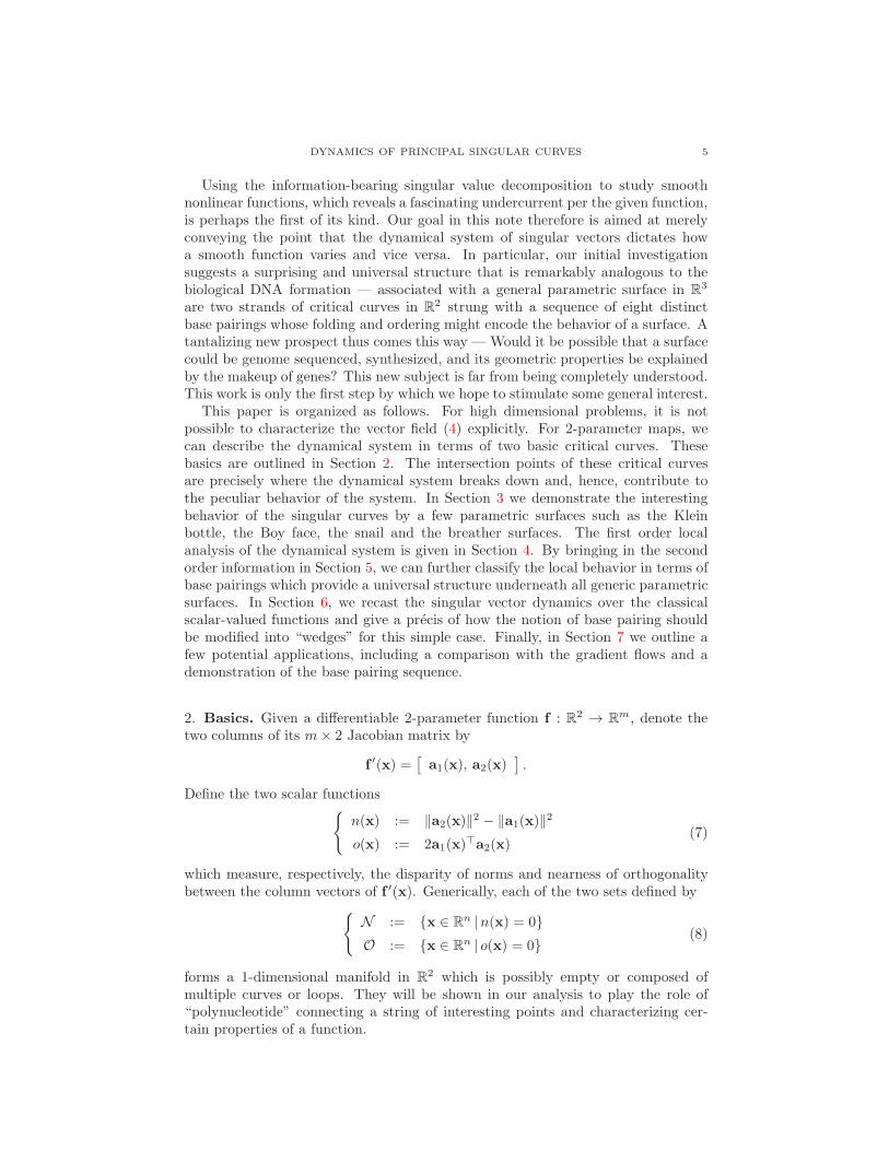
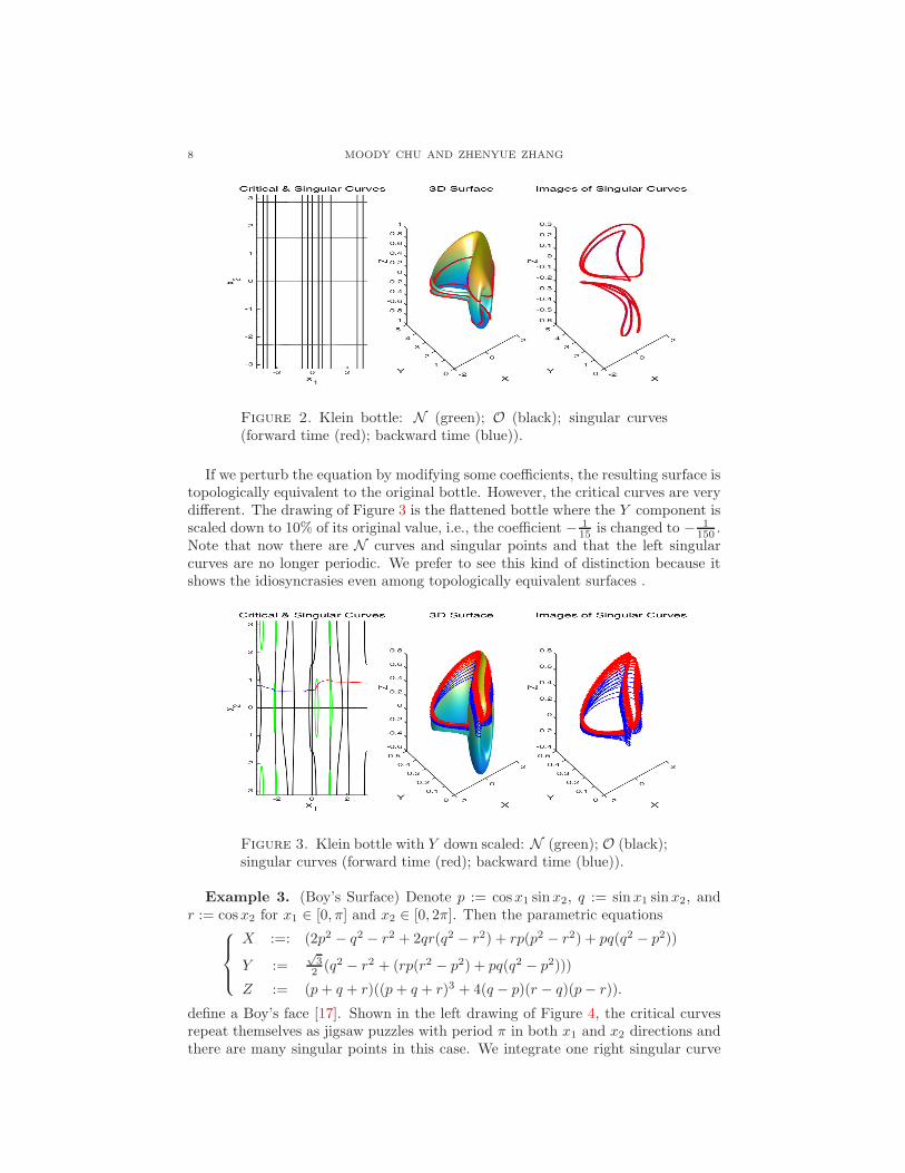
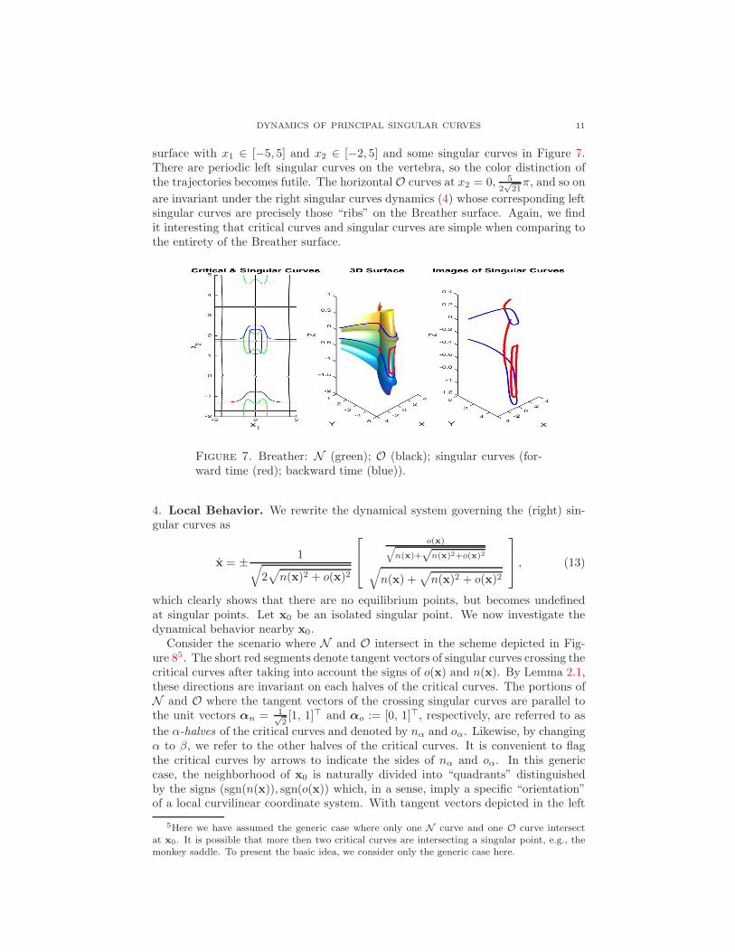
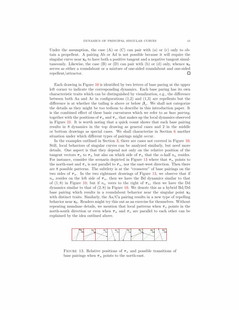1 Introduction The notion of nonlinear maps has been used in almost everyfield of disciplines as the most basic apparatus to describe complicated phenomenaHowever the metaphysical question of what impinges on a function in such a waythat we may make use of its variations to denote distinct episodes remain a naturalmystery Surface descriptions and their constructions in R

3 for example are ofcritical importance to a wide range of disciplines But what makes surfaces topresent so many different shapes and geometric properties This paper reportsa preliminary study of a dynamics system inbuilt in every function which mightsuggest an alternative interesting and possibly universal paradigm to help explorethese questions

Our idea is motivated by the gradient adaption which is ubiquitous in natureHeat transfer by conduction and osmosis of substances moving respectively oppo-site to the temperature gradient which is perpendicular to the isothermal surfacesand down a concentration gradient across the cell membrane without requiring en-ergy use are just two common examples typifying this natural process Gradientadaption follows the fundamental fact that the gradient

nablaη(x) =

[partη

partx1

partη

partxn

]

of a given smooth scalar function η Rn minusrarr R points in the steepest ascent directionfor the function value η(x) with the maximum rate exactly equal to the Euclideannorm nablaη(x) A mechanical generalization of the gradient of a scalar function toa smooth vector function f Rn minusrarr R

m should be the Jacobian matrix defined by

f prime(x) =

partf1partx1

partf1partxn

partfmpartx1

partfmpartxn

In this situation the information about how f(x) transforms itself is masked by thecombined effect of m gradients One way to quantify the variation of f is to measurethe rate of change along any given unit vector u via the norm of the directionalderivative

limtrarr0

∥∥∥∥f(x + tu)minus f(x)

t

∥∥∥∥ = f prime(x)u (1)

Similar to the gradient adaption we ask the question that along which directions thefunction f(x) changes most rapidly and how much the maximum rate is attainedThe answer lies in the notion of singular value decomposition (SVD) of the Jacobianmatrix f prime(x)

Any given matrix A isin Rmtimesn enjoys a factorization of the form

A = V ΣU⊤ (2)

where V isin Rmtimesm and U isin R

ntimesn are orthogonal matrices Σ isin Rmtimesn is zero

everywhere except for the nonnegative elements σ1 ge σ2 ge ge σκ gt σκ+1 = = 0 along the leading diagonal and κ = rank(A) The scalars σi and thecorresponding columns ui in U and vi in V are called the singular values the rightand the left singular vectors of A respectively [9] The notion of the SVD has longbeen conceived in various disciplines [22] as it appears frequently in a remarkablywide range of important applications mdash data analysis [6] dimension reduction [16]signal processing [23] image compression principal component analysis [24] to



maxu=1

Au (3)














yi(t) = f(xi(t)) (6)











3







]



o(x) = 2a1(x)⊤a2(x)

(7)


N = x isin R


n | o(x) = 0(8)





σ1(x) =(

12

(a1(x)2 + a2(x)2 +

radico(x)2 + n(x)2

))12

σ2(x) =(

12


radico(x)2 + n(x)2

))12

(9)


u1(x) =plusmn1radic

1 + ω(x)2

[ω(x)

1

] (10)

u2(x) =plusmn1radic

1 + ζ(x)2

[ζ(x)

1

] (11)

respectively where

ω(x) = o(x)

n(x)+radic

o(x)2+n(x)2


radico(x)2+n(x)2

o(x)

(12)



2[1 1]⊤ or βn = [1 minus1]⊤




2 defined by

f(x1 x2) =


]



2




minus4

minus3

minus2

minus1

0

1

2

3

4

5


x1

x 2

x1

x 2



minus4

minus3

minus2

minus1

0

1

2

3

4

5

x1

x 2



minus4

minus3

minus2

minus1

0

1

2

3

4

5








61 + 90s1c

41)


71s1 + 48c2c

61 minus 80c2c

51s1 minus 48c2c

41 minus 5c2c

31s1 minus 3c2c

21

+5s1c2c1 + 3c2 minus 60s1)

Z = 215s2(3 + 5s1c1)




















16 s = eminus1



X = r cos v


Z = r sin v








5 ((w cosh(25x1))2+(25 sin(wx2))


X = minusx1 +2w2


Y =2w cosh( 2

5x1)


Z =2w cosh( 2

5x1)












o(x)radic

n(x)+radic

n(x)2+o(x)2

radicn(x) +

radicn(x)2 + o(x)2

(13)







N

Ox0

(++)

(+minus)(minus+)

(minusminus) N

Ox0

(++)

(+minus)(minus+)

(minusminus)



N

O

x0

(++)

(+minus) (minus+)

(minusminus)

N

O

x0

(++)

(+minus) (minus+)

(minusminus)









DdDdCaCaCcCcDbDb


BbBb BdBd AaAa AcAc

BbBb BdBd AaAa AcAc








ω(x) =


sgn(o(x))n(x)2

2o(x)2+O

(n(x)3

) near n(x) = 0

o(x)2n(x) minus

o(x)3

8n(x)3 + o(x)5

16n(x)5 +O(o(x)


minus1o(x)2n(x)

minus o(x)3

8n(x)3+ o(x)5

16n(x)5+O(o(x)7)







(B) (D)(A) (C)

n(x) gt 0n(x) gt 0


n(x) lt 0

n(x) lt 0n(x) lt 0

x0x0 x0 x0

τn

τn τn

τn





(a) (c)(b) (d)

o(x) gt 0o(x) gt 0


o(x) lt 0


x0x0

τ o

τ o

τ o

τ o











Bd

Dd

Aa

Ca

Bb

Db Ca Cc

Aa Ac Ac

Cc

Bb

Ca

Bd

Dd




X = x1

Y = x2

Z = f(x1 x2)

(15)


n(x) =(

partfpartx2

)2

(x)minus(

partfpartx1

)2

(x)


(x) partfpartx2

(x)(16)


(x0) =partfpartx2


u1 = plusmn(12 +

(n+radicn2 + o2

o

)2)minus 1

2[

1n+

radicn2+o2

o

]= plusmn 1radic

partfpartx1

2+ partf

partx2

2

[partfpartx1

partfpartx2

]




(18)









n(x) gt 0

n(x) gt 0

n(x) gt 0

n(x) gt 0

n(x) gt 0

n(x) gt 0

n(x) gt 0

n(x) gt 0

n(x) lt 0

n(x) lt 0

n(x) lt 0

n(x) lt 0

n(x) lt 0

n(x) lt 0

n(x) lt 0

n(x) lt 0

x0x0x0x0


o(x) gt 0

o(x) gt 0

o(x) gt 0

o(x) gt 0

o(x) gt 0 o(x) gt 0

o(x) gt 0o(x) gt 0

o(x) lt 0

o(x) lt 0

o(x) lt 0

o(x) lt 0o(x) lt 0

o(x) lt 0

o(x) lt 0

o(x) lt 0

x0x0 x0x0

















x1

x 2



minus1

0

1

2

3

4 DdDb

CaCc

CcCa

DbDd

Aas

Bd

Bd

Ac

Aa

Ac

Bb

Bb

Ac

Ac

Bd

Bd

Aas

Bb

Ac

Bb







REFERENCES





































1 Introduction

2 Basics


4 Local Behavior

5 Base Pairing


7 Applications

8 Conclusion

REFERENCES



maxu=1

Au (3)














yi(t) = f(xi(t)) (6)











3







]



o(x) = 2a1(x)⊤a2(x)

(7)


N = x isin R


n | o(x) = 0(8)





σ1(x) =(

12

(a1(x)2 + a2(x)2 +

radico(x)2 + n(x)2

))12

σ2(x) =(

12


radico(x)2 + n(x)2

))12

(9)


u1(x) =plusmn1radic

1 + ω(x)2

[ω(x)

1

] (10)

u2(x) =plusmn1radic

1 + ζ(x)2

[ζ(x)

1

] (11)

respectively where

ω(x) = o(x)

n(x)+radic

o(x)2+n(x)2


radico(x)2+n(x)2

o(x)

(12)



2[1 1]⊤ or βn = [1 minus1]⊤




2 defined by

f(x1 x2) =


]



2




minus4

minus3

minus2

minus1

0

1

2

3

4

5


x1

x 2

x1

x 2



minus4

minus3

minus2

minus1

0

1

2

3

4

5

x1

x 2



minus4

minus3

minus2

minus1

0

1

2

3

4

5








61 + 90s1c

41)


71s1 + 48c2c

61 minus 80c2c

51s1 minus 48c2c

41 minus 5c2c

31s1 minus 3c2c

21

+5s1c2c1 + 3c2 minus 60s1)

Z = 215s2(3 + 5s1c1)




















16 s = eminus1



X = r cos v


Z = r sin v








5 ((w cosh(25x1))2+(25 sin(wx2))


X = minusx1 +2w2


Y =2w cosh( 2

5x1)


Z =2w cosh( 2

5x1)












o(x)radic

n(x)+radic

n(x)2+o(x)2

radicn(x) +

radicn(x)2 + o(x)2

(13)







N

Ox0

(++)

(+minus)(minus+)

(minusminus) N

Ox0

(++)

(+minus)(minus+)

(minusminus)



N

O

x0

(++)

(+minus) (minus+)

(minusminus)

N

O

x0

(++)

(+minus) (minus+)

(minusminus)









DdDdCaCaCcCcDbDb


BbBb BdBd AaAa AcAc

BbBb BdBd AaAa AcAc








ω(x) =


sgn(o(x))n(x)2

2o(x)2+O

(n(x)3

) near n(x) = 0

o(x)2n(x) minus

o(x)3

8n(x)3 + o(x)5

16n(x)5 +O(o(x)


minus1o(x)2n(x)

minus o(x)3

8n(x)3+ o(x)5

16n(x)5+O(o(x)7)







(B) (D)(A) (C)

n(x) gt 0n(x) gt 0


n(x) lt 0

n(x) lt 0n(x) lt 0

x0x0 x0 x0

τn

τn τn

τn





(a) (c)(b) (d)

o(x) gt 0o(x) gt 0


o(x) lt 0


x0x0

τ o

τ o

τ o

τ o











Bd

Dd

Aa

Ca

Bb

Db Ca Cc

Aa Ac Ac

Cc

Bb

Ca

Bd

Dd




X = x1

Y = x2

Z = f(x1 x2)

(15)


n(x) =(

partfpartx2

)2

(x)minus(

partfpartx1

)2

(x)


(x) partfpartx2

(x)(16)


(x0) =partfpartx2


u1 = plusmn(12 +

(n+radicn2 + o2

o

)2)minus 1

2[

1n+

radicn2+o2

o

]= plusmn 1radic

partfpartx1

2+ partf

partx2

2

[partfpartx1

partfpartx2

]




(18)









n(x) gt 0

n(x) gt 0

n(x) gt 0

n(x) gt 0

n(x) gt 0

n(x) gt 0

n(x) gt 0

n(x) gt 0

n(x) lt 0

n(x) lt 0

n(x) lt 0

n(x) lt 0

n(x) lt 0

n(x) lt 0

n(x) lt 0

n(x) lt 0

x0x0x0x0


o(x) gt 0

o(x) gt 0

o(x) gt 0

o(x) gt 0

o(x) gt 0 o(x) gt 0

o(x) gt 0o(x) gt 0

o(x) lt 0

o(x) lt 0

o(x) lt 0

o(x) lt 0o(x) lt 0

o(x) lt 0

o(x) lt 0

o(x) lt 0

x0x0 x0x0

















x1

x 2



minus1

0

1

2

3

4 DdDb

CaCc

CcCa

DbDd

Aas

Bd

Bd

Ac

Aa

Ac

Bb

Bb

Ac

Ac

Bd

Bd

Aas

Bb

Ac

Bb







REFERENCES





































1 Introduction

2 Basics


4 Local Behavior

5 Base Pairing


7 Applications

8 Conclusion

REFERENCES









3







]



o(x) = 2a1(x)⊤a2(x)

(7)


N = x isin R


n | o(x) = 0(8)





σ1(x) =(

12

(a1(x)2 + a2(x)2 +

radico(x)2 + n(x)2

))12

σ2(x) =(

12


radico(x)2 + n(x)2

))12

(9)


u1(x) =plusmn1radic

1 + ω(x)2

[ω(x)

1

] (10)

u2(x) =plusmn1radic

1 + ζ(x)2

[ζ(x)

1

] (11)

respectively where

ω(x) = o(x)

n(x)+radic

o(x)2+n(x)2


radico(x)2+n(x)2

o(x)

(12)



2[1 1]⊤ or βn = [1 minus1]⊤




2 defined by

f(x1 x2) =


]



2




minus4

minus3

minus2

minus1

0

1

2

3

4

5


x1

x 2

x1

x 2



minus4

minus3

minus2

minus1

0

1

2

3

4

5

x1

x 2



minus4

minus3

minus2

minus1

0

1

2

3

4

5








61 + 90s1c

41)


71s1 + 48c2c

61 minus 80c2c

51s1 minus 48c2c

41 minus 5c2c

31s1 minus 3c2c

21

+5s1c2c1 + 3c2 minus 60s1)

Z = 215s2(3 + 5s1c1)




















16 s = eminus1



X = r cos v


Z = r sin v








5 ((w cosh(25x1))2+(25 sin(wx2))


X = minusx1 +2w2


Y =2w cosh( 2

5x1)


Z =2w cosh( 2

5x1)












o(x)radic

n(x)+radic

n(x)2+o(x)2

radicn(x) +

radicn(x)2 + o(x)2

(13)







N

Ox0

(++)

(+minus)(minus+)

(minusminus) N

Ox0

(++)

(+minus)(minus+)

(minusminus)



N

O

x0

(++)

(+minus) (minus+)

(minusminus)

N

O

x0

(++)

(+minus) (minus+)

(minusminus)









DdDdCaCaCcCcDbDb


BbBb BdBd AaAa AcAc

BbBb BdBd AaAa AcAc








ω(x) =


sgn(o(x))n(x)2

2o(x)2+O

(n(x)3

) near n(x) = 0

o(x)2n(x) minus

o(x)3

8n(x)3 + o(x)5

16n(x)5 +O(o(x)


minus1o(x)2n(x)

minus o(x)3

8n(x)3+ o(x)5

16n(x)5+O(o(x)7)







(B) (D)(A) (C)

n(x) gt 0n(x) gt 0


n(x) lt 0

n(x) lt 0n(x) lt 0

x0x0 x0 x0

τn

τn τn

τn





(a) (c)(b) (d)

o(x) gt 0o(x) gt 0


o(x) lt 0


x0x0

τ o

τ o

τ o

τ o











Bd

Dd

Aa

Ca

Bb

Db Ca Cc

Aa Ac Ac

Cc

Bb

Ca

Bd

Dd




X = x1

Y = x2

Z = f(x1 x2)

(15)


n(x) =(

partfpartx2

)2

(x)minus(

partfpartx1

)2

(x)


(x) partfpartx2

(x)(16)


(x0) =partfpartx2


u1 = plusmn(12 +

(n+radicn2 + o2

o

)2)minus 1

2[

1n+

radicn2+o2

o

]= plusmn 1radic

partfpartx1

2+ partf

partx2

2

[partfpartx1

partfpartx2

]




(18)









n(x) gt 0

n(x) gt 0

n(x) gt 0

n(x) gt 0

n(x) gt 0

n(x) gt 0

n(x) gt 0

n(x) gt 0

n(x) lt 0

n(x) lt 0

n(x) lt 0

n(x) lt 0

n(x) lt 0

n(x) lt 0

n(x) lt 0

n(x) lt 0

x0x0x0x0


o(x) gt 0

o(x) gt 0

o(x) gt 0

o(x) gt 0

o(x) gt 0 o(x) gt 0

o(x) gt 0o(x) gt 0

o(x) lt 0

o(x) lt 0

o(x) lt 0

o(x) lt 0o(x) lt 0

o(x) lt 0

o(x) lt 0

o(x) lt 0

x0x0 x0x0

















x1

x 2



minus1

0

1

2

3

4 DdDb

CaCc

CcCa

DbDd

Aas

Bd

Bd

Ac

Aa

Ac

Bb

Bb

Ac

Ac

Bd

Bd

Aas

Bb

Ac

Bb







REFERENCES





































1 Introduction

2 Basics


4 Local Behavior

5 Base Pairing


7 Applications

8 Conclusion

REFERENCES



σ1(x) =(

12

(a1(x)2 + a2(x)2 +

radico(x)2 + n(x)2

))12

σ2(x) =(

12


radico(x)2 + n(x)2

))12

(9)


u1(x) =plusmn1radic

1 + ω(x)2

[ω(x)

1

] (10)

u2(x) =plusmn1radic

1 + ζ(x)2

[ζ(x)

1

] (11)

respectively where

ω(x) = o(x)

n(x)+radic

o(x)2+n(x)2


radico(x)2+n(x)2

o(x)

(12)



2[1 1]⊤ or βn = [1 minus1]⊤




2 defined by

f(x1 x2) =


]



2




minus4

minus3

minus2

minus1

0

1

2

3

4

5


x1

x 2

x1

x 2



minus4

minus3

minus2

minus1

0

1

2

3

4

5

x1

x 2



minus4

minus3

minus2

minus1

0

1

2

3

4

5








61 + 90s1c

41)


71s1 + 48c2c

61 minus 80c2c

51s1 minus 48c2c

41 minus 5c2c

31s1 minus 3c2c

21

+5s1c2c1 + 3c2 minus 60s1)

Z = 215s2(3 + 5s1c1)




















16 s = eminus1



X = r cos v


Z = r sin v








5 ((w cosh(25x1))2+(25 sin(wx2))


X = minusx1 +2w2


Y =2w cosh( 2

5x1)


Z =2w cosh( 2

5x1)












o(x)radic

n(x)+radic

n(x)2+o(x)2

radicn(x) +

radicn(x)2 + o(x)2

(13)







N

Ox0

(++)

(+minus)(minus+)

(minusminus) N

Ox0

(++)

(+minus)(minus+)

(minusminus)



N

O

x0

(++)

(+minus) (minus+)

(minusminus)

N

O

x0

(++)

(+minus) (minus+)

(minusminus)









DdDdCaCaCcCcDbDb


BbBb BdBd AaAa AcAc

BbBb BdBd AaAa AcAc








ω(x) =


sgn(o(x))n(x)2

2o(x)2+O

(n(x)3

) near n(x) = 0

o(x)2n(x) minus

o(x)3

8n(x)3 + o(x)5

16n(x)5 +O(o(x)


minus1o(x)2n(x)

minus o(x)3

8n(x)3+ o(x)5

16n(x)5+O(o(x)7)







(B) (D)(A) (C)

n(x) gt 0n(x) gt 0


n(x) lt 0

n(x) lt 0n(x) lt 0

x0x0 x0 x0

τn

τn τn

τn





(a) (c)(b) (d)

o(x) gt 0o(x) gt 0


o(x) lt 0


x0x0

τ o

τ o

τ o

τ o











Bd

Dd

Aa

Ca

Bb

Db Ca Cc

Aa Ac Ac

Cc

Bb

Ca

Bd

Dd




X = x1

Y = x2

Z = f(x1 x2)

(15)


n(x) =(

partfpartx2

)2

(x)minus(

partfpartx1

)2

(x)


(x) partfpartx2

(x)(16)


(x0) =partfpartx2


u1 = plusmn(12 +

(n+radicn2 + o2

o

)2)minus 1

2[

1n+

radicn2+o2

o

]= plusmn 1radic

partfpartx1

2+ partf

partx2

2

[partfpartx1

partfpartx2

]




(18)









n(x) gt 0

n(x) gt 0

n(x) gt 0

n(x) gt 0

n(x) gt 0

n(x) gt 0

n(x) gt 0

n(x) gt 0

n(x) lt 0

n(x) lt 0

n(x) lt 0

n(x) lt 0

n(x) lt 0

n(x) lt 0

n(x) lt 0

n(x) lt 0

x0x0x0x0


o(x) gt 0

o(x) gt 0

o(x) gt 0

o(x) gt 0

o(x) gt 0 o(x) gt 0

o(x) gt 0o(x) gt 0

o(x) lt 0

o(x) lt 0

o(x) lt 0

o(x) lt 0o(x) lt 0

o(x) lt 0

o(x) lt 0

o(x) lt 0

x0x0 x0x0

















x1

x 2



minus1

0

1

2

3

4 DdDb

CaCc

CcCa

DbDd

Aas

Bd

Bd

Ac

Aa

Ac

Bb

Bb

Ac

Ac

Bd

Bd

Aas

Bb

Ac

Bb







REFERENCES





































1 Introduction

2 Basics


4 Local Behavior

5 Base Pairing


7 Applications

8 Conclusion

REFERENCES




minus4

minus3

minus2

minus1

0

1

2

3

4

5


x1

x 2

x1

x 2



minus4

minus3

minus2

minus1

0

1

2

3

4

5

x1

x 2



minus4

minus3

minus2

minus1

0

1

2

3

4

5








61 + 90s1c

41)


71s1 + 48c2c

61 minus 80c2c

51s1 minus 48c2c

41 minus 5c2c

31s1 minus 3c2c

21

+5s1c2c1 + 3c2 minus 60s1)

Z = 215s2(3 + 5s1c1)




















16 s = eminus1



X = r cos v


Z = r sin v








5 ((w cosh(25x1))2+(25 sin(wx2))


X = minusx1 +2w2


Y =2w cosh( 2

5x1)


Z =2w cosh( 2

5x1)












o(x)radic

n(x)+radic

n(x)2+o(x)2

radicn(x) +

radicn(x)2 + o(x)2

(13)







N

Ox0

(++)

(+minus)(minus+)

(minusminus) N

Ox0

(++)

(+minus)(minus+)

(minusminus)



N

O

x0

(++)

(+minus) (minus+)

(minusminus)

N

O

x0

(++)

(+minus) (minus+)

(minusminus)









DdDdCaCaCcCcDbDb


BbBb BdBd AaAa AcAc

BbBb BdBd AaAa AcAc








ω(x) =


sgn(o(x))n(x)2

2o(x)2+O

(n(x)3

) near n(x) = 0

o(x)2n(x) minus

o(x)3

8n(x)3 + o(x)5

16n(x)5 +O(o(x)


minus1o(x)2n(x)

minus o(x)3

8n(x)3+ o(x)5

16n(x)5+O(o(x)7)







(B) (D)(A) (C)

n(x) gt 0n(x) gt 0


n(x) lt 0

n(x) lt 0n(x) lt 0

x0x0 x0 x0

τn

τn τn

τn





(a) (c)(b) (d)

o(x) gt 0o(x) gt 0


o(x) lt 0


x0x0

τ o

τ o

τ o

τ o











Bd

Dd

Aa

Ca

Bb

Db Ca Cc

Aa Ac Ac

Cc

Bb

Ca

Bd

Dd




X = x1

Y = x2

Z = f(x1 x2)

(15)


n(x) =(

partfpartx2

)2

(x)minus(

partfpartx1

)2

(x)


(x) partfpartx2

(x)(16)


(x0) =partfpartx2


u1 = plusmn(12 +

(n+radicn2 + o2

o

)2)minus 1

2[

1n+

radicn2+o2

o

]= plusmn 1radic

partfpartx1

2+ partf

partx2

2

[partfpartx1

partfpartx2

]




(18)









n(x) gt 0

n(x) gt 0

n(x) gt 0

n(x) gt 0

n(x) gt 0

n(x) gt 0

n(x) gt 0

n(x) gt 0

n(x) lt 0

n(x) lt 0

n(x) lt 0

n(x) lt 0

n(x) lt 0

n(x) lt 0

n(x) lt 0

n(x) lt 0

x0x0x0x0


o(x) gt 0

o(x) gt 0

o(x) gt 0

o(x) gt 0

o(x) gt 0 o(x) gt 0

o(x) gt 0o(x) gt 0

o(x) lt 0

o(x) lt 0

o(x) lt 0

o(x) lt 0o(x) lt 0

o(x) lt 0

o(x) lt 0

o(x) lt 0

x0x0 x0x0

















x1

x 2



minus1

0

1

2

3

4 DdDb

CaCc

CcCa

DbDd

Aas

Bd

Bd

Ac

Aa

Ac

Bb

Bb

Ac

Ac

Bd

Bd

Aas

Bb

Ac

Bb







REFERENCES





































1 Introduction

2 Basics


4 Local Behavior

5 Base Pairing


7 Applications

8 Conclusion

REFERENCES
















16 s = eminus1



X = r cos v


Z = r sin v








5 ((w cosh(25x1))2+(25 sin(wx2))


X = minusx1 +2w2


Y =2w cosh( 2

5x1)


Z =2w cosh( 2

5x1)












o(x)radic

n(x)+radic

n(x)2+o(x)2

radicn(x) +

radicn(x)2 + o(x)2

(13)







N

Ox0

(++)

(+minus)(minus+)

(minusminus) N

Ox0

(++)

(+minus)(minus+)

(minusminus)



N

O

x0

(++)

(+minus) (minus+)

(minusminus)

N

O

x0

(++)

(+minus) (minus+)

(minusminus)









DdDdCaCaCcCcDbDb


BbBb BdBd AaAa AcAc

BbBb BdBd AaAa AcAc








ω(x) =


sgn(o(x))n(x)2

2o(x)2+O

(n(x)3

) near n(x) = 0

o(x)2n(x) minus

o(x)3

8n(x)3 + o(x)5

16n(x)5 +O(o(x)


minus1o(x)2n(x)

minus o(x)3

8n(x)3+ o(x)5

16n(x)5+O(o(x)7)







(B) (D)(A) (C)

n(x) gt 0n(x) gt 0


n(x) lt 0

n(x) lt 0n(x) lt 0

x0x0 x0 x0

τn

τn τn

τn





(a) (c)(b) (d)

o(x) gt 0o(x) gt 0


o(x) lt 0


x0x0

τ o

τ o

τ o

τ o











Bd

Dd

Aa

Ca

Bb

Db Ca Cc

Aa Ac Ac

Cc

Bb

Ca

Bd

Dd




X = x1

Y = x2

Z = f(x1 x2)

(15)


n(x) =(

partfpartx2

)2

(x)minus(

partfpartx1

)2

(x)


(x) partfpartx2

(x)(16)


(x0) =partfpartx2


u1 = plusmn(12 +

(n+radicn2 + o2

o

)2)minus 1

2[

1n+

radicn2+o2

o

]= plusmn 1radic

partfpartx1

2+ partf

partx2

2

[partfpartx1

partfpartx2

]




(18)









n(x) gt 0

n(x) gt 0

n(x) gt 0

n(x) gt 0

n(x) gt 0

n(x) gt 0

n(x) gt 0

n(x) gt 0

n(x) lt 0

n(x) lt 0

n(x) lt 0

n(x) lt 0

n(x) lt 0

n(x) lt 0

n(x) lt 0

n(x) lt 0

x0x0x0x0


o(x) gt 0

o(x) gt 0

o(x) gt 0

o(x) gt 0

o(x) gt 0 o(x) gt 0

o(x) gt 0o(x) gt 0

o(x) lt 0

o(x) lt 0

o(x) lt 0

o(x) lt 0o(x) lt 0

o(x) lt 0

o(x) lt 0

o(x) lt 0

x0x0 x0x0

















x1

x 2



minus1

0

1

2

3

4 DdDb

CaCc

CcCa

DbDd

Aas

Bd

Bd

Ac

Aa

Ac

Bb

Bb

Ac

Ac

Bd

Bd

Aas

Bb

Ac

Bb







REFERENCES





































1 Introduction

2 Basics


4 Local Behavior

5 Base Pairing


7 Applications

8 Conclusion

REFERENCES






5 ((w cosh(25x1))2+(25 sin(wx2))


X = minusx1 +2w2


Y =2w cosh( 2

5x1)


Z =2w cosh( 2

5x1)












o(x)radic

n(x)+radic

n(x)2+o(x)2

radicn(x) +

radicn(x)2 + o(x)2

(13)







N

Ox0

(++)

(+minus)(minus+)

(minusminus) N

Ox0

(++)

(+minus)(minus+)

(minusminus)



N

O

x0

(++)

(+minus) (minus+)

(minusminus)

N

O

x0

(++)

(+minus) (minus+)

(minusminus)









DdDdCaCaCcCcDbDb


BbBb BdBd AaAa AcAc

BbBb BdBd AaAa AcAc








ω(x) =


sgn(o(x))n(x)2

2o(x)2+O

(n(x)3

) near n(x) = 0

o(x)2n(x) minus

o(x)3

8n(x)3 + o(x)5

16n(x)5 +O(o(x)


minus1o(x)2n(x)

minus o(x)3

8n(x)3+ o(x)5

16n(x)5+O(o(x)7)







(B) (D)(A) (C)

n(x) gt 0n(x) gt 0


n(x) lt 0

n(x) lt 0n(x) lt 0

x0x0 x0 x0

τn

τn τn

τn





(a) (c)(b) (d)

o(x) gt 0o(x) gt 0


o(x) lt 0


x0x0

τ o

τ o

τ o

τ o











Bd

Dd

Aa

Ca

Bb

Db Ca Cc

Aa Ac Ac

Cc

Bb

Ca

Bd

Dd




X = x1

Y = x2

Z = f(x1 x2)

(15)


n(x) =(

partfpartx2

)2

(x)minus(

partfpartx1

)2

(x)


(x) partfpartx2

(x)(16)


(x0) =partfpartx2


u1 = plusmn(12 +

(n+radicn2 + o2

o

)2)minus 1

2[

1n+

radicn2+o2

o

]= plusmn 1radic

partfpartx1

2+ partf

partx2

2

[partfpartx1

partfpartx2

]




(18)









n(x) gt 0

n(x) gt 0

n(x) gt 0

n(x) gt 0

n(x) gt 0

n(x) gt 0

n(x) gt 0

n(x) gt 0

n(x) lt 0

n(x) lt 0

n(x) lt 0

n(x) lt 0

n(x) lt 0

n(x) lt 0

n(x) lt 0

n(x) lt 0

x0x0x0x0


o(x) gt 0

o(x) gt 0

o(x) gt 0

o(x) gt 0

o(x) gt 0 o(x) gt 0

o(x) gt 0o(x) gt 0

o(x) lt 0

o(x) lt 0

o(x) lt 0

o(x) lt 0o(x) lt 0

o(x) lt 0

o(x) lt 0

o(x) lt 0

x0x0 x0x0

















x1

x 2



minus1

0

1

2

3

4 DdDb

CaCc

CcCa

DbDd

Aas

Bd

Bd

Ac

Aa

Ac

Bb

Bb

Ac

Ac

Bd

Bd

Aas

Bb

Ac

Bb







REFERENCES





































1 Introduction

2 Basics


4 Local Behavior

5 Base Pairing


7 Applications

8 Conclusion

REFERENCES








o(x)radic

n(x)+radic

n(x)2+o(x)2

radicn(x) +

radicn(x)2 + o(x)2

(13)







N

Ox0

(++)

(+minus)(minus+)

(minusminus) N

Ox0

(++)

(+minus)(minus+)

(minusminus)



N

O

x0

(++)

(+minus) (minus+)

(minusminus)

N

O

x0

(++)

(+minus) (minus+)

(minusminus)









DdDdCaCaCcCcDbDb


BbBb BdBd AaAa AcAc

BbBb BdBd AaAa AcAc








ω(x) =


sgn(o(x))n(x)2

2o(x)2+O

(n(x)3

) near n(x) = 0

o(x)2n(x) minus

o(x)3

8n(x)3 + o(x)5

16n(x)5 +O(o(x)


minus1o(x)2n(x)

minus o(x)3

8n(x)3+ o(x)5

16n(x)5+O(o(x)7)







(B) (D)(A) (C)

n(x) gt 0n(x) gt 0


n(x) lt 0

n(x) lt 0n(x) lt 0

x0x0 x0 x0

τn

τn τn

τn





(a) (c)(b) (d)

o(x) gt 0o(x) gt 0


o(x) lt 0


x0x0

τ o

τ o

τ o

τ o











Bd

Dd

Aa

Ca

Bb

Db Ca Cc

Aa Ac Ac

Cc

Bb

Ca

Bd

Dd




X = x1

Y = x2

Z = f(x1 x2)

(15)


n(x) =(

partfpartx2

)2

(x)minus(

partfpartx1

)2

(x)


(x) partfpartx2

(x)(16)


(x0) =partfpartx2


u1 = plusmn(12 +

(n+radicn2 + o2

o

)2)minus 1

2[

1n+

radicn2+o2

o

]= plusmn 1radic

partfpartx1

2+ partf

partx2

2

[partfpartx1

partfpartx2

]




(18)









n(x) gt 0

n(x) gt 0

n(x) gt 0

n(x) gt 0

n(x) gt 0

n(x) gt 0

n(x) gt 0

n(x) gt 0

n(x) lt 0

n(x) lt 0

n(x) lt 0

n(x) lt 0

n(x) lt 0

n(x) lt 0

n(x) lt 0

n(x) lt 0

x0x0x0x0


o(x) gt 0

o(x) gt 0

o(x) gt 0

o(x) gt 0

o(x) gt 0 o(x) gt 0

o(x) gt 0o(x) gt 0

o(x) lt 0

o(x) lt 0

o(x) lt 0

o(x) lt 0o(x) lt 0

o(x) lt 0

o(x) lt 0

o(x) lt 0

x0x0 x0x0

















x1

x 2



minus1

0

1

2

3

4 DdDb

CaCc

CcCa

DbDd

Aas

Bd

Bd

Ac

Aa

Ac

Bb

Bb

Ac

Ac

Bd

Bd

Aas

Bb

Ac

Bb







REFERENCES





































1 Introduction

2 Basics


4 Local Behavior

5 Base Pairing


7 Applications

8 Conclusion

REFERENCES


N

Ox0

(++)

(+minus)(minus+)

(minusminus) N

Ox0

(++)

(+minus)(minus+)

(minusminus)



N

O

x0

(++)

(+minus) (minus+)

(minusminus)

N

O

x0

(++)

(+minus) (minus+)

(minusminus)









DdDdCaCaCcCcDbDb


BbBb BdBd AaAa AcAc

BbBb BdBd AaAa AcAc








ω(x) =


sgn(o(x))n(x)2

2o(x)2+O

(n(x)3

) near n(x) = 0

o(x)2n(x) minus

o(x)3

8n(x)3 + o(x)5

16n(x)5 +O(o(x)


minus1o(x)2n(x)

minus o(x)3

8n(x)3+ o(x)5

16n(x)5+O(o(x)7)







(B) (D)(A) (C)

n(x) gt 0n(x) gt 0


n(x) lt 0

n(x) lt 0n(x) lt 0

x0x0 x0 x0

τn

τn τn

τn





(a) (c)(b) (d)

o(x) gt 0o(x) gt 0


o(x) lt 0


x0x0

τ o

τ o

τ o

τ o











Bd

Dd

Aa

Ca

Bb

Db Ca Cc

Aa Ac Ac

Cc

Bb

Ca

Bd

Dd




X = x1

Y = x2

Z = f(x1 x2)

(15)


n(x) =(

partfpartx2

)2

(x)minus(

partfpartx1

)2

(x)


(x) partfpartx2

(x)(16)


(x0) =partfpartx2


u1 = plusmn(12 +

(n+radicn2 + o2

o

)2)minus 1

2[

1n+

radicn2+o2

o

]= plusmn 1radic

partfpartx1

2+ partf

partx2

2

[partfpartx1

partfpartx2

]




(18)









n(x) gt 0

n(x) gt 0

n(x) gt 0

n(x) gt 0

n(x) gt 0

n(x) gt 0

n(x) gt 0

n(x) gt 0

n(x) lt 0

n(x) lt 0

n(x) lt 0

n(x) lt 0

n(x) lt 0

n(x) lt 0

n(x) lt 0

n(x) lt 0

x0x0x0x0


o(x) gt 0

o(x) gt 0

o(x) gt 0

o(x) gt 0

o(x) gt 0 o(x) gt 0

o(x) gt 0o(x) gt 0

o(x) lt 0

o(x) lt 0

o(x) lt 0

o(x) lt 0o(x) lt 0

o(x) lt 0

o(x) lt 0

o(x) lt 0

x0x0 x0x0

















x1

x 2



minus1

0

1

2

3

4 DdDb

CaCc

CcCa

DbDd

Aas

Bd

Bd

Ac

Aa

Ac

Bb

Bb

Ac

Ac

Bd

Bd

Aas

Bb

Ac

Bb







REFERENCES





































1 Introduction

2 Basics


4 Local Behavior

5 Base Pairing


7 Applications

8 Conclusion

REFERENCES




DdDdCaCaCcCcDbDb


BbBb BdBd AaAa AcAc

BbBb BdBd AaAa AcAc








ω(x) =


sgn(o(x))n(x)2

2o(x)2+O

(n(x)3

) near n(x) = 0

o(x)2n(x) minus

o(x)3

8n(x)3 + o(x)5

16n(x)5 +O(o(x)


minus1o(x)2n(x)

minus o(x)3

8n(x)3+ o(x)5

16n(x)5+O(o(x)7)







(B) (D)(A) (C)

n(x) gt 0n(x) gt 0


n(x) lt 0

n(x) lt 0n(x) lt 0

x0x0 x0 x0

τn

τn τn

τn





(a) (c)(b) (d)

o(x) gt 0o(x) gt 0


o(x) lt 0


x0x0

τ o

τ o

τ o

τ o











Bd

Dd

Aa

Ca

Bb

Db Ca Cc

Aa Ac Ac

Cc

Bb

Ca

Bd

Dd




X = x1

Y = x2

Z = f(x1 x2)

(15)


n(x) =(

partfpartx2

)2

(x)minus(

partfpartx1

)2

(x)


(x) partfpartx2

(x)(16)


(x0) =partfpartx2


u1 = plusmn(12 +

(n+radicn2 + o2

o

)2)minus 1

2[

1n+

radicn2+o2

o

]= plusmn 1radic

partfpartx1

2+ partf

partx2

2

[partfpartx1

partfpartx2

]




(18)









n(x) gt 0

n(x) gt 0

n(x) gt 0

n(x) gt 0

n(x) gt 0

n(x) gt 0

n(x) gt 0

n(x) gt 0

n(x) lt 0

n(x) lt 0

n(x) lt 0

n(x) lt 0

n(x) lt 0

n(x) lt 0

n(x) lt 0

n(x) lt 0

x0x0x0x0


o(x) gt 0

o(x) gt 0

o(x) gt 0

o(x) gt 0

o(x) gt 0 o(x) gt 0

o(x) gt 0o(x) gt 0

o(x) lt 0

o(x) lt 0

o(x) lt 0

o(x) lt 0o(x) lt 0

o(x) lt 0

o(x) lt 0

o(x) lt 0

x0x0 x0x0

















x1

x 2



minus1

0

1

2

3

4 DdDb

CaCc

CcCa

DbDd

Aas

Bd

Bd

Ac

Aa

Ac

Bb

Bb

Ac

Ac

Bd

Bd

Aas

Bb

Ac

Bb







REFERENCES





































1 Introduction

2 Basics


4 Local Behavior

5 Base Pairing


7 Applications

8 Conclusion

REFERENCES





(B) (D)(A) (C)

n(x) gt 0n(x) gt 0


n(x) lt 0

n(x) lt 0n(x) lt 0

x0x0 x0 x0

τn

τn τn

τn





(a) (c)(b) (d)

o(x) gt 0o(x) gt 0


o(x) lt 0


x0x0

τ o

τ o

τ o

τ o











Bd

Dd

Aa

Ca

Bb

Db Ca Cc

Aa Ac Ac

Cc

Bb

Ca

Bd

Dd




X = x1

Y = x2

Z = f(x1 x2)

(15)


n(x) =(

partfpartx2

)2

(x)minus(

partfpartx1

)2

(x)


(x) partfpartx2

(x)(16)


(x0) =partfpartx2


u1 = plusmn(12 +

(n+radicn2 + o2

o

)2)minus 1

2[

1n+

radicn2+o2

o

]= plusmn 1radic

partfpartx1

2+ partf

partx2

2

[partfpartx1

partfpartx2

]




(18)









n(x) gt 0

n(x) gt 0

n(x) gt 0

n(x) gt 0

n(x) gt 0

n(x) gt 0

n(x) gt 0

n(x) gt 0

n(x) lt 0

n(x) lt 0

n(x) lt 0

n(x) lt 0

n(x) lt 0

n(x) lt 0

n(x) lt 0

n(x) lt 0

x0x0x0x0


o(x) gt 0

o(x) gt 0

o(x) gt 0

o(x) gt 0

o(x) gt 0 o(x) gt 0

o(x) gt 0o(x) gt 0

o(x) lt 0

o(x) lt 0

o(x) lt 0

o(x) lt 0o(x) lt 0

o(x) lt 0

o(x) lt 0

o(x) lt 0

x0x0 x0x0

















x1

x 2



minus1

0

1

2

3

4 DdDb

CaCc

CcCa

DbDd

Aas

Bd

Bd

Ac

Aa

Ac

Bb

Bb

Ac

Ac

Bd

Bd

Aas

Bb

Ac

Bb







REFERENCES





































1 Introduction

2 Basics


4 Local Behavior

5 Base Pairing


7 Applications

8 Conclusion

REFERENCES







Bd

Dd

Aa

Ca

Bb

Db Ca Cc

Aa Ac Ac

Cc

Bb

Ca

Bd

Dd




X = x1

Y = x2

Z = f(x1 x2)

(15)


n(x) =(

partfpartx2

)2

(x)minus(

partfpartx1

)2

(x)


(x) partfpartx2

(x)(16)


(x0) =partfpartx2


u1 = plusmn(12 +

(n+radicn2 + o2

o

)2)minus 1

2[

1n+

radicn2+o2

o

]= plusmn 1radic

partfpartx1

2+ partf

partx2

2

[partfpartx1

partfpartx2

]




(18)









n(x) gt 0

n(x) gt 0

n(x) gt 0

n(x) gt 0

n(x) gt 0

n(x) gt 0

n(x) gt 0

n(x) gt 0

n(x) lt 0

n(x) lt 0

n(x) lt 0

n(x) lt 0

n(x) lt 0

n(x) lt 0

n(x) lt 0

n(x) lt 0

x0x0x0x0


o(x) gt 0

o(x) gt 0

o(x) gt 0

o(x) gt 0

o(x) gt 0 o(x) gt 0

o(x) gt 0o(x) gt 0

o(x) lt 0

o(x) lt 0

o(x) lt 0

o(x) lt 0o(x) lt 0

o(x) lt 0

o(x) lt 0

o(x) lt 0

x0x0 x0x0

















x1

x 2



minus1

0

1

2

3

4 DdDb

CaCc

CcCa

DbDd

Aas

Bd

Bd

Ac

Aa

Ac

Bb

Bb

Ac

Ac

Bd

Bd

Aas

Bb

Ac

Bb







REFERENCES





































1 Introduction

2 Basics


4 Local Behavior

5 Base Pairing


7 Applications

8 Conclusion

REFERENCES



X = x1

Y = x2

Z = f(x1 x2)

(15)


n(x) =(

partfpartx2

)2

(x)minus(

partfpartx1

)2

(x)


(x) partfpartx2

(x)(16)


(x0) =partfpartx2


u1 = plusmn(12 +

(n+radicn2 + o2

o

)2)minus 1

2[

1n+

radicn2+o2

o

]= plusmn 1radic

partfpartx1

2+ partf

partx2

2

[partfpartx1

partfpartx2

]




(18)









n(x) gt 0

n(x) gt 0

n(x) gt 0

n(x) gt 0

n(x) gt 0

n(x) gt 0

n(x) gt 0

n(x) gt 0

n(x) lt 0

n(x) lt 0

n(x) lt 0

n(x) lt 0

n(x) lt 0

n(x) lt 0

n(x) lt 0

n(x) lt 0

x0x0x0x0


o(x) gt 0

o(x) gt 0

o(x) gt 0

o(x) gt 0

o(x) gt 0 o(x) gt 0

o(x) gt 0o(x) gt 0

o(x) lt 0

o(x) lt 0

o(x) lt 0

o(x) lt 0o(x) lt 0

o(x) lt 0

o(x) lt 0

o(x) lt 0

x0x0 x0x0

















x1

x 2



minus1

0

1

2

3

4 DdDb

CaCc

CcCa

DbDd

Aas

Bd

Bd

Ac

Aa

Ac

Bb

Bb

Ac

Ac

Bd

Bd

Aas

Bb

Ac

Bb







REFERENCES





































1 Introduction

2 Basics


4 Local Behavior

5 Base Pairing


7 Applications

8 Conclusion

REFERENCES


n(x) gt 0

n(x) gt 0

n(x) gt 0

n(x) gt 0

n(x) gt 0

n(x) gt 0

n(x) gt 0

n(x) gt 0

n(x) lt 0

n(x) lt 0

n(x) lt 0

n(x) lt 0

n(x) lt 0

n(x) lt 0

n(x) lt 0

n(x) lt 0

x0x0x0x0


o(x) gt 0

o(x) gt 0

o(x) gt 0

o(x) gt 0

o(x) gt 0 o(x) gt 0

o(x) gt 0o(x) gt 0

o(x) lt 0

o(x) lt 0

o(x) lt 0

o(x) lt 0o(x) lt 0

o(x) lt 0

o(x) lt 0

o(x) lt 0

x0x0 x0x0

















x1

x 2



minus1

0

1

2

3

4 DdDb

CaCc

CcCa

DbDd

Aas

Bd

Bd

Ac

Aa

Ac

Bb

Bb

Ac

Ac

Bd

Bd

Aas

Bb

Ac

Bb







REFERENCES





































1 Introduction

2 Basics


4 Local Behavior

5 Base Pairing


7 Applications

8 Conclusion

REFERENCES











x1

x 2



minus1

0

1

2

3

4 DdDb

CaCc

CcCa

DbDd

Aas

Bd

Bd

Ac

Aa

Ac

Bb

Bb

Ac

Ac

Bd

Bd

Aas

Bb

Ac

Bb







REFERENCES





































1 Introduction

2 Basics


4 Local Behavior

5 Base Pairing


7 Applications

8 Conclusion

REFERENCES





























1 Introduction

2 Basics


4 Local Behavior

5 Base Pairing


7 Applications

8 Conclusion

REFERENCES

the dynamics of principal singular curves: an innate ... · moody chu∗ department of mathematics...

Documents