Marshall UniversityMarshall Digital Scholar

Theses, Dissertations and Capstones

2006

The Dynamics of Newton's Method on CubicPolynomialsShannon N. Miller

Follow this and additional works at: http://mds.marshall.edu/etdPart of the Dynamical Systems Commons, Non-linear Dynamics Commons, and the Other

Mathematics Commons

This Thesis is brought to you for free and open access by Marshall Digital Scholar. It has been accepted for inclusion in Theses, Dissertations andCapstones by an authorized administrator of Marshall Digital Scholar. For more information, please contact zhangj@marshall.edu.

Recommended CitationMiller, Shannon N., "The Dynamics of Newton's Method on Cubic Polynomials" (2006). Theses, Dissertations and Capstones. Paper758.

THE DYNAMICS OF NEWTON’S METHOD ON CUBIC

POLYNOMIALS

Thesis submitted to

The Graduate College of

Marshall University

In partial fulfillment of the

Requirements for the degree of

Master of Arts

Department of Mathematics

by

Shannon N. Miller

Dr. Ralph Oberste-Vorth, Committee Chairman

Dr. Ariyadasa Aluthge

Dr. Evelyn Pupplo-Cody

Marshall University

May 2006

ABSTRACT

THE DYNAMICS OF NEWTON’S METHOD ON CUBIC

POLYNOMIALS

By Shannon N. Miller

The field of dynamics is itself a huge part of many branches of science, including

the motion of the planets and galaxies, changing weather patterns, and the growth

and decline of populations. Consider a function f and pick x0 in the domain of f . If

we iterate this function around the point x0, then we will have the sequence x0, f(x0),

f(f(x0)), f(f(f(x0))), ..., which becomes our dynamical system. We are essentially

interested in the end behavior of this system. Do we have convergence? Does it

diverge? Could it do neither? We will focus on the functions obtained with Newton’s

method on polynomials and will apply our knowledge of dynamics. We also will be

studying the types of graphs one would get if they looked at these same functions in

the complex plane.

ACKNOWLEDGEMENTS

The author wishes to acknowledge the contributions of the following people:

My committee:

Dr. Aluthge, who taught me in three semesters just how much I like complex

variables and integral equations. He also took the time to sit down and really discuss

the material in this work. Thank you.

Dr. Oberste-Vorth whose knowledge, time, and effort has been put forth to help

me understand a subject in which I really enjoy begin involved. Even with the loss of

a loved one, he managed to take the time out and help me finish this paper on time.

Kudos.

Dr. Pupplo-Cody, who did not hesitate to talk to a crying freshman when she was

crushed with an ever so slightly imperfect grade in her first college math course, has

put forth so much effort into completely understanding my topic and giving me new

ideas to make the presentation so much more inviting to watch. Thanks.

Also, Dr. Lawrence, my graduate advisor and mentor, was always there for me

when I was in need. Whether it be a math problem or wanting to learn to ballroom

dance, this is your woman!

To my fiance Rob-Roy, thank you for supporting me through stressful times. I love

you.

Finally, to my grandmother, the person that wanted nothing more for me in life

than to be a better person. Mamaw, I am.

iii

Contents

1 Preliminaries 1

1.1 Chaotic Dynamics . . . . . . . . . . . . . . . . . . . . . . . . . . . . . . 1

1.2 The Mandlebrot, Julia and Fatou Sets . . . . . . . . . . . . . . . . . . 7

2 Newton’s Method 11

2.1 An Interation . . . . . . . . . . . . . . . . . . . . . . . . . . . . . . . . 11

2.2 Conjugacy Classes of Quadratics . . . . . . . . . . . . . . . . . . . . . . 15

3 Newton’s Method Extended 23

3.1 Cubics . . . . . . . . . . . . . . . . . . . . . . . . . . . . . . . . . . . . 23

3.2 Conjugacy Classes of Cubics . . . . . . . . . . . . . . . . . . . . . . . . 24

4 Graphical Analysis 31

4.1 The Symmetry of Nλ . . . . . . . . . . . . . . . . . . . . . . . . . . . . 31

4.2 Newton’s Method for Cubic Polynomial Nλ . . . . . . . . . . . . . . . . 38

A MatLab Code 43

A.1 Newton’s Method on Quadratic Polynomials . . . . . . . . . . . . . . . 43

A.2 Newton’s Method on Cubic Polynomials . . . . . . . . . . . . . . . . . 45

A.3 Newton’s Method on Lambda Cubic . . . . . . . . . . . . . . . . . . . 47

A.4 Parameterspace . . . . . . . . . . . . . . . . . . . . . . . . . . . . . . . 49

iv

List of Figures

2.1 Newton’s method on the quadratic polynomial p(z) = z2 − 2z − 3. . . . 20

2.2 Newton’s method on the quadratic polynomial p(z) = z2 − 2.5. . . . . . 20

3.1 Newton’s method a generic polynomial with three roots for initial guess

x0. . . . . . . . . . . . . . . . . . . . . . . . . . . . . . . . . . . . . . . 23

4.1 Newton’s method on the cubic polynomial p(z) = z3 + z2 + z +1. Here,

λ = i. . . . . . . . . . . . . . . . . . . . . . . . . . . . . . . . . . . . . 33

4.2 The parameter space created with z = 13. . . . . . . . . . . . . . . . . . 39

4.3 Excerpt from parameter space figure. . . . . . . . . . . . . . . . . . . . 40

4.4 The set of periodic points from our parameter space. . . . . . . . . . . 40

4.5 Nλ for λ = .589 + 605i from -1.5 to 1.5. . . . . . . . . . . . . . . . . . . 41

4.6 Nλ for λ = .589 + .605i from 0 to 1.5. . . . . . . . . . . . . . . . . . . . 41

4.7 “The Rabbit”: Nλ for λ = .589 + .605i from 0.2 to .48. . . . . . . . . . 42

v

Chapter 1

Preliminaries

1.1 Chaotic Dynamics

What exactly is a dynamical system? These systems involve iterating a mathematical

function and then asking what happens. No one really knows the answer to this

question...completely. Even with such simple functions as the quadratic or cubic, no

one can say precisely what would happen.

We will be considering specific functions and their behaviors. For example, we will

consider the following functions:

1. f1(x) = x2

2. f2(x) = x3

3. f3(x) = sin x

4. f4(x) = 1x

Let us begin by looking at a few preliminaries. We can think about this iteration

process as one you would take if you were finding the square root or the square, by

repeating an action over and over again. This list of iterates around a point is called

the orbit of that point. We can define the orbit in a recursive manner, i.e. f 0(x) = x

and for all n ∈ N, fn(x) = f(fn−1(x)). However, we employ the following definition.

Definition 1 (Orbit) Let f(x) be a function defined on a domain. The orbit of the

function, denoted fn(x), for a point x is created by iterating a function starting at that

1

point to get a list of numbers. The forward orbit of x is the set of points in the sequence

x, f(x), f(f(x)), f(f(f(x))), written more succinctly as x, f(x), f 2(x), f 3(x),... and

will be denoted fn(x) for n ∈ N. Similarly, the backward orbit of x is the set of points

in the sequence x, f−1(x), f−1(f−1(x)), f−1(f−1(f−1(x))), written more succinctly as

x, f−1(x), f−2(x), f−3(x),... and will be denoted by f−n(x) for n ∈ N whenever the

inverses exist.

For the case when f1(x) = x2, depending on the position of the point that you

pick, i.e. 0 < |x| < 1, |x| > 1, x = 1, x = −1, or x = 0, there will be a possibility

of three different types of behavior of the orbit for that specific point. The first type

of behavior we will see is convergence. This is when the orbit of a particular point

approaches a finite value when we iterate the function infinitely, or fn(x) → 0 as

n → ∞. The other two are divergence, fn(x) → ∞ as n → ∞, and having fixed

points, fn(x) = 1 or fn(x) = 0 for all n. In the latter case, we can say that the point

does not “move” over the iterate. This gives us the following definition.

Definition 2 (Fixed Point) The point x is a fixed point for f if f(x) = x. We will

denote the set of all fixed points as Fix(x).

Suppose x0 is a fixed point of an analytic function f , that is, f(x0) = x0. The

number λ = f′(x0), where f

′is the derivative of f , is called the multiplier of f at x0.

A possible reason for being called a multiplier is because of its position is the equation

used for the Mean Value Theorem |f(x)−f(y)| = f′(x)|x−y|. We classify fixed points

according to λ as follows:

Superattracting : λ = 0.

Attracting : |λ| < 1.

Repelling : |λ| > 1.

Rationally neutral : |λ| = 1 and λn = 1 for some integer n.

Irrationally neutral : |λ| = 1 but λn is never 1.

If we choose a point that may not be a fixed point, we find that other points in

the plane exhibit these same characteristics. We will concentrate on the first three

2

properties right now, because the last two properties on the list only occur when we

have a complex function.

Now, let us take a look at f3(x) = sin x. Consider the point x0=1.57. We see that

the first few iterates are approximately

f3(1.57) = .999

f 23 (1.57) = .841

f 33 (1.57) = .745

f 43 (1.57) = .678

and the points are decreasing on the average by .107. If we jump a few iterations

ahead,

f 733 (1.57) = .197

f 743 (1.57) = .196

f 753 (1.57) = .194

the average decrease is .0015. Even further, we have

f 2983 (1.57) = .099527

f 2993 (1.57) = .099362

f 3003 (1.57) = .099199

As we can see, this is slowly approaching 0, which is a fixed point for this function.

These iterations are getting closer and closer to 0, and thus we say this point, x0 = 1.57

is attracted to zero. So, we would call x0 = 1.57 a convergent point. Furthermore,

our second function f2 illustrates this property. We can see immediately that zero is a

fixed point. Also, ±1 are fixed points. So, let us pick some points between these with

3

which we have discussed. If we choose x0 = −1.5, x0 = −.5, x0 = .5, and x0 = 1.5,

then we will get the following chart of iterations.

Iteration x0 = −1.5 x0 = −.5 x0 = .5 x0 = 1.5

f2(x) -3.375 -.125 .125 3.375

f 22 (x) -38.4434 -.0019 .0019 38.4434

f 32 (x) -56815.3088 −7.450× 10−9 7.450× 10−9 56815.3088

f 42 (x) −1.8340× 1014 −4.1359× 10−25 4.1359× 10−25 1.8340× 1014

f 52 (x) −6.1688× 1042 −7.0747× 10−74 7.0747× 10−74 6.1688× 1042

The points chosen in the interval from -1 to 0 and the interval 0 to 1 are attracted

to zero very quickly. In this case, zero is a super-attractive fixed point, since f′(0) = 0.

However, if we look at the point chosen to the left of the fixed point -1, as well at the

point chosen to the right of 1, these two iterations seem to push away from each of

their corresponding fixed points. This tells us that that if we keep iterating we will

approach infinity. When the iterations tend to infinity, the points -1 and 1 are called

repelling fixed points, since |f ′(−1)| = 3 and |f ′(1)| = 3.

However, let us choose a point for f4(x) = 1x. We would like to find all the fixed

points, i.e. all the points that satisfy the equation 1x

= x. This is equivalent to solving

the equation 1 = x2. We can see that the only two points that will satisfy this equation

are x = 1 and x = −1. If we choose a nonzero number between -1 and 1, say .5, and

iterate it, we see that the first few iterates are,

f4(.5) = 2

f 24 (.5) = .5

f 34 (.5) = 2

f 44 (.5) = .5

where the points seem to repeat a “cycle” of numbers that includes the original. We

4

call this iterate a periodic orbit, or cycle. If we jump a few iterations ahead,

f 734 (.5) = 2

f 744 (.5) = .5

f 754 (.5) = 2

the orbit is still the same. We say that .5 is a periodic point of period 2, since the

cycle repeats the value of .5 every second iterate. We expect this behavior from the

recursiveness of our iteration. This gives us another definition.

Definition 3 (Periodic Point) The point x is a periodic point for f if fn(x) = x,

for some integer n. The least positive n for which fn(x) = x is called the prime period

of x. We will denote the set of periodic points of period n by Pern(f)

In this case, every nonzero point in the interval that contains .5, i.e. (−1, 1), will

be a periodic point of period 2. There are two types of periodic points: hyperbolic

and non-hyperbolic. We will be dealing with hyperbolic periodic points unless told

otherwise, but what does it mean to be hyperbolic?

Definition 4 (Hyperbolic) Let p be a periodic point of prime period n. The point

p is hyperbolic if |(fn)′(p)| 6= 1. The number (fn)′(p) is called the multiplier of the

periodic point.

One important thing about these hyperbolic periodic points is the fact that if we

pick some other point that is relatively close to them, the orbit of that particular point

will converge to the hyperbolic periodic point. Note that a fixed point is a periodic

point. The following proposition illustrates this idea.

Proposition 1 Let f be C1 and p be a hyperbolic fixed point with |f ′(p)| < 1. Then

there is an open interval U about the hyperbolic fixed point p ∈ U such that if x ∈ U ,

then

limn→∞

fn(x) = p.

5

Proof. Since f is C1, f′(x) exists and is continuous at all x in some interval U

about p. So, there is ε > 0 small enough and A ∈ R+ so that |f ′(x)| < A < 1 when

x ∈ [p−ε, p+ε] and 0 < A < 1. Since p is a fixed point of f , we know that |f(x)−p| =|f(x)− f(p)|, and from the definition of the derivative f

′(x) = limn→∞

f(x)−f(p)x−p

. From

the Mean Value Theorem we have that |f(x) − f(p)| < A|x − p|. Using our previous

statement, we have the following

|f(x)− p| = |f(x)− f(p)| < A|x− p| < |x− p| ≤ ε,

since x is in the ε-ball around p. Hence f(x) is contained in [p− ε, p + ε] and, in fact,

is closer to p than x is. Via the same argument

|fn(x)− p| < An|x− p|

so that fn(x) → p as n →∞. ¤

The previous proposition leads us to the following definition about the points

around a particular x0.

Definition 5 (Basin of Attraction) The set of all points whose orbits are attractive

periodic orbits is the basin of attraction of that orbit.

So far we have only been considering points in the the real line. We have seen all the

different types of behavior that occur at these points. What about complex numbers

in the complex plane? Suppose we are given a complex-valued function g : C → C

defined as

g(x, y) = u(x, y) + iv(x, y)

where u and v are maps from R2 to R. Again, we are interested in the behavior of

orbit of g at a particular point.

One thing that we will discuss is the graphical nature of these complex iterates

which create beautiful pictures called fractals. When we graph these, we simply graph

6

the real part in the horizontal direction and the imaginary part in the vertical direction.

We now dive into the realm of the complex chaotic dynamics.

1.2 The Mandlebrot, Julia and Fatou Sets

It is useful to think of the iteration of a function being defined on the Riemann sphere,

C, consisting of the complex plane with a point at infinity. We know that looking at

the complex plane will open up solutions that we would not have in the real x − y

plane. Any complex differentiable map f : C → C on the Riemann sphere can be

expressed as a rational function, that is as the quotient,

f(z) =p(z)

q(z),

where p and q are polynomials. In this case, we have to assume that p and q have no

common roots. The degree, d, of f is equal to the largest the degrees of p and q.

The global study of Newton’s method can now be analyzed using this theory of

complex dynamics of rational maps on this Riemann sphere. Any complex analytical

mapping will decompose the plane into two complementing sets, the stable set, where

the dynamics are mostly tame, and the unstable set, where the dynamics become

chaotic and unpredictable. The study of this idea was started by G. Julia and P.

Fatou in the 1920’s. Let us take a look at some of their findings.

We start out by examining some of the special properties of maps defined in the

complex plane. In fact, it is these properties that give the dynamics of complex analytic

mappings a much richer structure that we previously mentioned.

Definition 6 (Normal Family) For a function F , the family F n of iterates is a

normal family on an open set U if every sequence of the F n’s has a subsequence which

either

1. converges uniformly on compact subsets of U , or

2. converges uniformly to ∞ on U .

7

If you let R(z) be a rational function, where

R(z) =P (z)

Q(z).

Here P and Q are polynomials that have no common factors and d =max(deg(P ),

deg(Q))≥ 2. The Fatou set F of R is defined to be the set of points z0 ∈ C such that

Rn is a normal family in some neighborhood of z0. The Julia set J is the complement

of the Fatou set. The Julia Set is the boundary of the sets that escape, i.e. those that

do not converge, and those that never escape, i.e. those that do converge.

As an example, consider the squaring map f : z → z2. The entire open unit disk

D is contained in the Fatou set of f , since successive iterates on any compact subset

of D converge uniformly to zero. Similarly, the exterior, C \ D is contained in the

Fatou set, since the iterates of f converge to the constant function z →∞ outside of

D. On the other hand, if z0 belongs to the unit circle, then in any neighborhood of

z0 any limit of iterates fn would necessarily have a jump discontinuity as we cross the

unit circle. We arrive to the very descriptive definition of the Julia set.

Definition 7 Consider a complex mapping of the form zn+1 = f(zn). The points that

lie of the boundary between points that are bounded and those that are unbounded are

collectively referred to as the Julia set. The following properties of a Julia set, J , are

well known:

• The set J is invariant.

• An orbit on J is either periodic or eventually periodic.

• All repelling periodic points are on J . So, set J is a repellor.

• The set J is either connected or totally disconnected.

• The set J nearly always has fractal structure.

If we have a polynomial, the Julia set is the closure of the set of all repelling

periodic points. Let us explore what Julia and Fatou discovered by considering once

8

again the square function f1(x) = x2. In R, we have observed that if |x| < 1, then

fn(x) → 0, and |x| > 1, then fn(x) →∞. The map has only two fixed points and all

other points eventually approach one of them or go off to infinity. Thus, we can say

that the dynamics are fairly tame. If we translate this to the complex plane, the set

of all attracting convergent points is contained in the open unit disk, and the set of

all repelling divergent points are on the outside of the closure of this same disk. This

tells us that the Julia set is precisely equal to the unit circle.

To summarize, we have to following definition.

Definition 8 Let S be a Riemann surface, let f : S → S be a non-constant holomor-

phic, or analytic, mapping, and let fn be its nth-interate, or orbit. Fixing some point

z0 ∈ S, we have the dichotomy(a mutually exclusive bipartition of elements): If there

exists some neighborhood U of z0 so that the sequence of iterates fn restricted to U

forms a normal family, then we say that z0 is a regular or normal point, or that z0

belongs to the Fatou set of f. Otherwise, if no such neighborhood exists, we say that z0

belongs to the Julia set.

Now that we have a few definitions under our belts, let us look at a few facts about

these two sets. Julia sets define the border between bounded and unbounded orbits.

Now, the Julia set associated with the point c = a + ib is denoted by Jc.

Theorem 1 Every attracting periodic orbit is contained in the Fatou set. In fact the

entire basin of attraction Ω for an attracting periodic orbit is contained in the Fatou

set. However the boundary of the basin ∂Ω is contained in the Julia set, and every

repelling periodic orbit is contained in the Julia set.

Proof. We need only consider the case of a fixed point. If z0 is attracting, the

it follows from Taylor’s Theorem that the successive iterates of f , restricted to a

small neighborhood of z0, converge uniformly to the constant function z → z0. The

corresponding statement for any compact subset of the basin Ω then follow easily.

On the other hand, around a boundary point of this basin, that is, a point which

9

belongs to the closure Ω but not to Ω itself, it is clear that no sequence of iterates

can converge to a continuous limit. If z0 is repelling, then no sequence of iterates can

converge uniformly near z0, since the derivative dfn(z)dz

at z0 takes the value λn, which

diverges to infinity as n →∞. ¤

The previous theorem leads us to the following conclusion. If we define the basin

of attraction of z0 for a rational map R(z), A(z0) = z ∈ C : Rn(z) → z0. This

notation allows for another definition of the Julia set in the following theorem.

Theorem 2 For P (z) with deg(P ) ≥ 2, the boundary of A(z) coincides with the Julia

set of P .

Proof. From Theorem 1, we see that ∂A(z) ∈ J(P ). Suppose w0 is on the boundary

of ∂A(z) and V is any neighborhood of w0. Then for z0 ∈ A(z)⋂

V , P n(z) →∞, but

the orbit of w0, P n(w0) remains bounded. Thus P n is not normal in V so w0 is in the

Julia set.¤

Looking ahead in our studies, it is with this theorem that we will see the complexity

in the case of the cubic, which in turn adds character to the iteration of the complex

function. This theorem simply says that all the basins have the same boundary. So,

if we have the case of three attracting fixed points, then any disk that intersects two

of the basins must intersect all the basins.

Only when we iterate these functions in the complex plane will we see the Man-

delbrot set. It is the set of complex numbers c for which the iteration zn+1 = zn + c

produces finite zn for all n. The Mandelbrot set is seen when we choose to color the

points of the plane according to their convergence to the root. We will see more of

this in chapters to come. For different parameter values of the Mandelbrot set, we will

show the many different forms of the Julia set.

10

Chapter 2

Newton’s Method

2.1 An Interation

Newton’s method is used to calculate approximately the roots of any real-valued dif-

ferentiable function. Newton’s method is the best known iteration method for finding

these real and/or complex roots. We begin with an initial point, say x0, on the real

axis. Using the point (x0, f(x0)), we can obtain the equation for the tangent line at

this point, and it is

y − f(x0) = f ′(x0)(x− x0).

If we let the x-intercept of this line be the point x1, we have the following equation

−f(x0) = f ′(x0)(x1 − x0).

Solving this equation for x1, we obtain

x1 = x0 − f(x0)

f ′(x0).

Now, repeat the same steps using our new point x1 to get x2. Continuing these same

actions recursively, we will be able to represent our pattern as

xn+1 = xn − f(xn)

f ′(xn)

11

where f ′(xn) 6= 0. What we want to do is observe the behavior after iteration. As

n → ∞, this system exhibits several possible behaviors. The first and most trivial

is where x0 is a root of the polynomial f , and here we see that xn = x0 for all n.

The orbit in this case will look like x0, x0, x0, .... The second type of behavior occurs

when x0 is not a root of our polynomial and f ′(x0) = 0. This tells us that we cannot

use Newton’s Method, and our orbit will will go off, or converge, to infinity. In the

third type, if in the orbit one of the previous points is repeated, we will have a cycling

behavior in which none of the points are roots. In other words, xn = x0 for some n.

Again, this sequence does not converge, nor does it diverge. So, we will refer to this

as periodic, and the points in the orbit will be our periodic points. Other points will

simply fail to converge.

We will be considering throughout the remainder of our discussion the following

function defining Newton’s Method on a map f : C→ C

Nf (z) = z − f(z)

f ′(z).

Starting with some initial approximate value z0, we define the (n + 1) approximation

by zn+1 = Nf (zn). If the function is a polynomial (or a rational function), then the

iteration function Nf , after some manipulation, will be a rational map of the form

Np(z) =p(z)

q(z)

where p and q are polynomials with real or complex coefficients.

Aside from the particular dynamics of Newton’s Method, one goal is to discover

the relationship between any particular polynomial and it’s Newton function. This

leads us to the definition of topological conjugacy.

Definition 9 Let f : A → A and g : B → B be two functions, i.e. the original

polynomial p and the function created after applying Newton’s Method. These two

functions are called topologically conjugate if there exists a homeomorphism m that

12

maps A → B such that the following diagram commutes.

Af−−−→ A

m

y m

yB

g−−−→ B

The basin of attraction for a root of a polynomial is the set of starting points

which eventually converge to this root. Since every root is at least an attracting or

even a super-attracting fixed point, this basin includes a neighborhood of the root and

is non-empty.

So what is the relationship between fixed points of Newton’s method and points

of the original function? The roots of any polynomial equation are the fixed points of

the Newton function. One would think that these points should be of some interest

in the beginning function, i.e., possibly critical points of the original function? This

is sometimes true, however, the following proposition describes the relationship when

the roots are not critical points, the points where the function and/or its derivative is

equal to zero.

Proposition 2 Given an analytic function f whose roots are not critical points of f ,

then the roots of f are superattractive fixed points of Nf .

Proof. Let r be any root of f such that f′(r) 6= 0. Then,

Nf (r) = r − f(r)

f ′(r)= r

since r is a root of f , or f(r) = 0, and f′

does not vanish at r, or f′(r) 6= 0. We

conclude that r is a fixed point of Nf by the definition of fixed point. Now, if we look

at the derivative,

N′f (r) = 1− f

′(r)f

′(r)− f(r)f

′′(r)

(f ′(r))2

=(f

′(r))2 − (f

′(r))2 + f(r)f

′′(r)

(f ′(r))2

13

=f(r)f

′′(r)

(f ′(r))2.

For the same reasons as given for Nf (r) = r, the multiplier, which we have discussed

before, is λ = N′f (r) = 0, we have that r is a superattracting fixed point of Nf . ¤

What about those functions whose roots are in fact critical points of the original

equation? We should be able to say something stronger about these points. In fact,

we have another proposition that has a particular claim about these particular points.

Proposition 3 Given an analytic function f whose roots are critical points of f , then

the roots of f are attractive fixed points of Nf such that the N′f (r) = n−1

nwhere r is

the root and n is the order of that root.

Proof. Let r be a zero of order n ≥ 2 for f . We then take the Taylor series represen-

tation of f about r. The first n− 1 terms of f vanish at r, so

f(z) =f (n)(r)

n!(z − r)n +

f (n)(r)

(n + 1)!(z − r)n+1 + . . .

N′f (r) = lim

z→r

f(z)f′′(z)

(f ′(z))2

= limz→r

(f (n)(r)

n!(z − r)n + . . .

)(f (n)(r)(n−2)!

(z − r)n−2 + . . .)

(f (n)(r)(n−1)!

(z − r)n−1 + . . .)2

= limz→r

(fn(r))2

n!(n−2)!(z − r)2n−2 + . . .

(fn(r))2

((n−1)!)2(z − r)2n−2 + . . .

Dividing the numerator and denominator by the greatest common factor (z−r)2n−2

and applying the limit yields the following leading coefficients of N′f (r).

(fn(r))2

n!(n−2)!

(fn(r))2

((n−1)!)2

=n− 1

n.

14

Thus, r is an attractive fixed point for Nf . ¤

2.2 Conjugacy Classes of Quadratics

Let us consider once again the square function, but this time as a complex function.

Here, f(z) = z2, where z = x + iy is a complex number. In terms of its real and

imaginary parts, f(x+ iy) = x2−y2 + i(2xy), so f(z) is also a complex number. From

this, we can say that the orbit of any complex number with this function will be a

complex number. If we iterate f , will we see many of the same types of behavior?

We begin by working with functions of the type zn+1 = z2n + c. Thus we can say

that

xn+1 = x2n − y2

n + a,

and

yn+1 = 2xnyn + b,

are the real and imaginary parts, where zn = xn + iyn and c = a+ ib. We need to look

at the inverse mapping of this function in order to utilize the properties. To do this

one must find expressions for xn and yn in terms of xn+1 and yn+1. Now,

x2n − y2

n = xn+1 − a.

Also, note that

(x2n + y2

n)2 = (x2n − y2

n)2 + 4x2ny2

n

= (x2n − y2

n + a− a)2 + (2xnyn + b− b)2

= (xn+1 − a)2 + (yn+1 − b)2,

and hence,

x2n + y2

n = +√

(xn+1 − a)2 + (yn+1 − b)2,

15

since x2n + y2

n > 0. Let

u =√

(x2n − y2

n)2 + (2xnyn)2 and v = x2n − y2

n.

Then,

xn = ±√

u + v

2and yn =

yn+1 − b

2xn

.

In terms of the computation, there will be a problem if xn = 0. To overcome this

difficulty, the following simple algorithm is applied. Suppose that the two roots of

equation are given by x1 + iy1 and x2 + iy2. If x1 =√

u+v2

, then y1 =√

u− v if y > b,

or y1 = −√u− v if y < b. The other root is then given by x2 = −√

u+v2

and y2 = −y1.

It is not hard to determine the fixed points for mapping zn+1 = fc(zn) = z2n + c.

Suppose that z is a fixed point of period one. Then zn+1 = zn = z, and

z2 − z + c = 0,

which gives us two solutions,

z1 =1 +

√1− 4c

2

or

z2 =1−√1− 4c

2.

The stability of these fixed points can be determined in the usual way. Hence the fixed

point is stable if for fc = z2 − z + c

∣∣∣∣dfc

dz

∣∣∣∣ < 1,

and it is unstable if ∣∣∣∣dfc

dz

∣∣∣∣ > 1.

As a simple example, let us consider

zn+1 = z2n.

16

This is exactly the same as before, except this time we are in the complex plane. One

of two fixed points of the equation lies at the origin. Call it z∗, and there is also a

fixed point at z = 1. Initial points that start inside the unit circle are attracted to z∗,

i.e. an initial point starting on |z| = 1 will generate points that again lie on |z| = 1.

The initial points starting outside the |z| = 1 will be repelled to infinity, since |z| > 1.

Therefore, the circle defines the Julia set J that is a repellor, invariant, and connected.

The interior of |z| = 1 defines the basin of attraction (or domain of stability) for the

fixed point at z∗.

Since we know so much about this simple complex quadratic, it would be nice if

we could compare any general complex quadratic. We can in fact do this and show

that these two polynomials behave the same dynamically.

Theorem 3 Any complex quadratic polynomial f is conjugate to exactly one polyno-

mial in the one parameter family gc : z → z2 + c.

Proof. Let f(z) = az2 + bz + d represent a general quadratic. Let gc(z) = z2 + c

and define h(z) = Az + B, A,B 6= 0. From the definition of topological conjugacy, we

want to find A and B such that h f = g h . The commutativity of this expression

depends of the equality of the two equations

(h f)(z) = Aaz2 + Abz + Ad + B,

(gc h)(z) = A2z2 + 2ABz + B2 + c.

If we set each of the corresponding coefficients of both equations equal to one another,

it yields the following three equations

Aa = A2

Ab = 2AB

Ad + B = B2 + c.

17

Solving the first two equations, we see that A = a and B = b/2, whence we obtain

that f is topologically conjugate to the family gc, denoted by f ∼ gc, via the affine

transformation

h(z) = az +b

2

and on the condition that the third equation be satisfied, i.e.

c = ad +b

2− b2

4.

¤

In Propositions 2 and 3, we saw that the behavior of Newton’s method is different

when considering two different types of roots, ones that are critical points and those

that are not. What are some other traits that distinguish roots of polynomials? Well,

some quadratics have roots that are the same. For example, consider the quadratic

f(z) = z2 − 6zi − 9. Here, f(z) can be factored such that we can see its roots

f(z) = (z − 3i)(z − 3i). In this case, f(z) does not have two distinct roots, but one

root of multiplicity two. Is the behavior of Newton’s method different for the roots

that are distinct as opposed to the ones that are not distinct? The subsequent lemma

illustrates part of the answer.

Lemma 1 The Newton function of a general quadratic, f , with two distinct roots is

conjugate to the Newton function of gc : z → z2 + c for some nonzero c.

Proof. Denoting Newton’s method on f(z) = az2 + bz + d and Newton’s method on

gc(z) = z2 + c for c 6= 0 as the functions

Nf (z) =az2 − d

2az + band Ngc(z) =

z2 − c

2z,

respectively, let’s determine a conjugating map, k(z) = Az + B, such that

(k Nf )(z) = A

(az2 − d

2az + b

)+ B =

Aaz2 − Ad + 2Bza + Bb

2az + b

18

and

(Ngc k)(z) =(Az + B)2 − c

2(Az + B)=

A2z2 + 2ABz + B2 − c

2(Az + B)

Again, we want to set these two expression equal to one another and solve. This means

cross multiplying the two rational functions to get these two expressions:

2aA2z3 + 6aABz2 + (4aB2 + 2bAB − 2dA2)z + 2bB2 − 2dAB

and

2aA2z3 + (bA2 + 4aAB)z2 + (2aB2 − 2ac + 2bAB)z + bB2 − bc.

For the z3 terms we get the tautology 2aA2 = 2aA2. The z2 term yields

6AaB = 4AaB + A2b

2AaB = A2b

B =A2b

2Aa=

Ab

2a.

We find c = A2d−aB2

aby comparing the coefficients of the z terms. Since A is any

arbitrary non-zero value, we can choose A = 1 to get the general solution k(z) = z+ b2a

with c = − b2−4ad4a2 . ¤

Let us look at an example of this behavior. First, consider the quadratic f(z) =

z2− 2z− 3 and its conjugate function g(z) = z2− 2.5. We can see, in Figures 2.1 and

2.2, the rate of convergence for each point around the roots of the polynomial. The

picture generated with f and that of g show exactly the same behavior.

19

Figure 2.1: Newton’s method on the quadratic polynomial p(z) = z2 − 2z − 3.

Figure 2.2: Newton’s method on the quadratic polynomial p(z) = z2 − 2.5.

We have seen that Newton’s method of any general quadratic is conjugate to New-

ton’s method of some polynomial in the one parameter family z2 + c. Can we make

this any easier? As a matter of fact, the next lemma takes what we have shown and

makes it even simpler.

Lemma 2 Newton’s method on gc : z → z2 + c for some nonzero c is conjugate to the

simple quadratic g0 = z2 + 0.

20

Proof. Recall that Ngc(z) = z2−c2z

. We will express our conjugating map as a Mobius

transformation rather than as an affine map. Given l(z) = Az+BCz+D

, we want to find

A,B, C, and D such that l g0 = Ngc l. Well,

(l Ngc)(z) =Az2 − Ac + 2Bz

Cz2 − Cc + 2Dzand (g0 l)(z) =

A2z2 − 2ABz + B2

Cz + D2.

Cross multiplying these rational functions gives the following

AC2z4 + (2BC2 + 2ADC)z3 + (4BDC −AcC2−AD2)z2 + 2BD2− 2AcDC)z−AcD2

and

CA2z4 + (2DA + 2CAB)z3 + (4DAB − CcA2 + CB2)z2 + (2DB2 − 2CcAB)zCcB2.

One can verify that we get A = C 6= 0, B = ±D 6= 0 as general solutions where

c = −D2

C2 ; however, we exclude the solution B = D since that makes the conjugating

map, l, a constant function. Since, c = −D2

C2 , so DC

= ±i√

c. For DC

= ±i√

c, we get

hc(z) = z−i√

cz+i

√c

conjugating ngc to g0. If DC

= −i√

c, then our conjugating map is of the

form hc(z) = z+i√

cz−i

√c. ¤

In this case, the point we start with in our iteration always converges to the nearest

root. Also, the Julia set is the line created with the perpendicular bisector of the two

roots. If we tried to “measure” this line, we would see a measure of zero. In other

words, there is no girth to the Julia set. This line divides the plane into two symmetric

parts. In Chapters 3 and 4, we will see that this is not the case.

We have really simplified the way we look at Newton’s method on a general

quadratic. The only way that this would be any easier for us is if these functions

were conjugate to some linear function. The next theorem exemplifies this.

Theorem 4 Suppose f has an attracting fixed point at z0, with multiplier λ satisfying

0 < |λ| < 1. Then there is a conformal map ζ = ϕ(z) of a neighborhood of z0 onto

a neighborhood of 0 which conjugates f(z) to the linear function g(ζ) = λζ. The

21

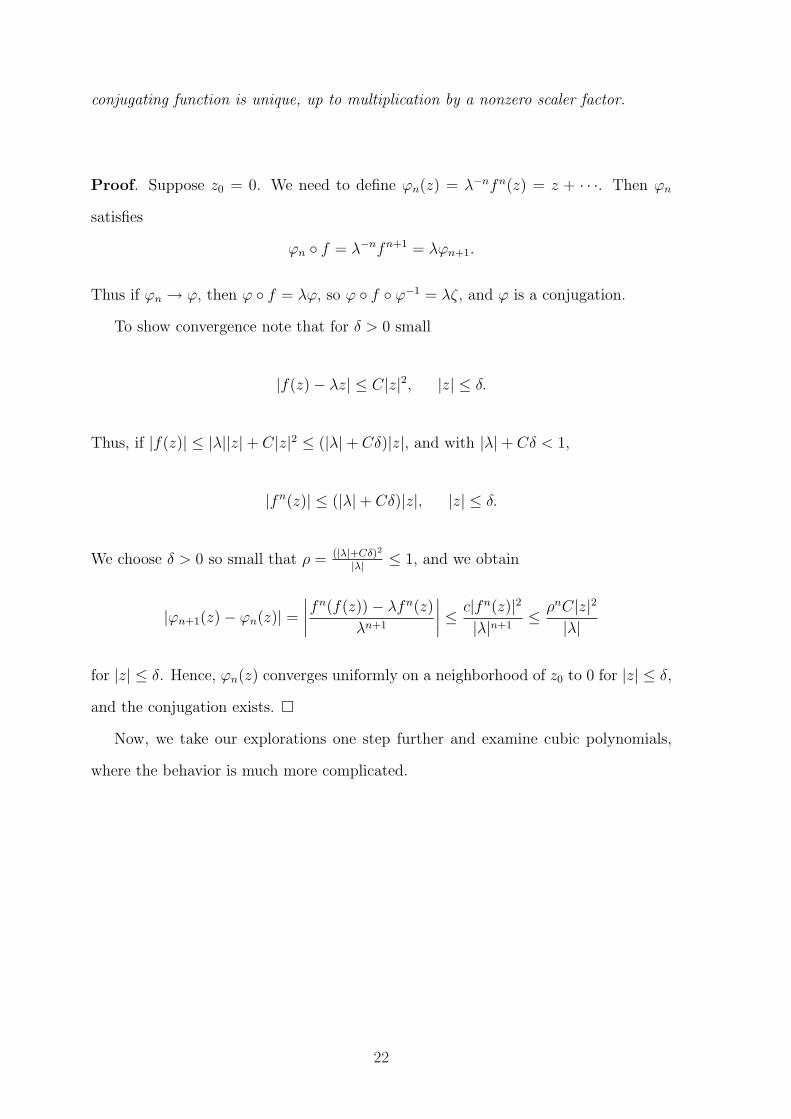
conjugating function is unique, up to multiplication by a nonzero scaler factor.

Proof. Suppose z0 = 0. We need to define ϕn(z) = λ−nfn(z) = z + · · ·. Then ϕn

satisfies

ϕn f = λ−nfn+1 = λϕn+1.

Thus if ϕn → ϕ, then ϕ f = λϕ, so ϕ f ϕ−1 = λζ, and ϕ is a conjugation.

To show convergence note that for δ > 0 small

|f(z)− λz| ≤ C|z|2, |z| ≤ δ.

Thus, if |f(z)| ≤ |λ||z|+ C|z|2 ≤ (|λ|+ Cδ)|z|, and with |λ|+ Cδ < 1,

|fn(z)| ≤ (|λ|+ Cδ)|z|, |z| ≤ δ.

We choose δ > 0 so small that ρ = (|λ|+Cδ)2

|λ| ≤ 1, and we obtain

|ϕn+1(z)− ϕn(z)| =∣∣∣∣fn(f(z))− λfn(z)

λn+1

∣∣∣∣ ≤c|fn(z)|2|λ|n+1

≤ ρnC|z|2|λ|

for |z| ≤ δ. Hence, ϕn(z) converges uniformly on a neighborhood of z0 to 0 for |z| ≤ δ,

and the conjugation exists. ¤

Now, we take our explorations one step further and examine cubic polynomials,

where the behavior is much more complicated.

22

Chapter 3

Newton’s Method Extended

3.1 Cubics

Consider the generic polnomial in Figure 3.1. Here we can see that a particular initial

guess need not converge to the nearest root. By Theorem 2 of Chapter 1, the Julia set

must be a complicated fractal set when there are more than two basins of attraction.

Figure 3.1: Newton’s method a generic polynomial with three roots for initial guessx0.

We know that a polynomial is most generally represented as

f(z) = anzn + an−1zn−1 + . . . + a1z + a0,

which is the exact way we have been viewing the quadratics in the previous chapter.

23

It is also known that we can view this same polynomial in terms of its roots

f(z) = an(z − r1)(z − r2) · · · (z − rn)

where r1, r2, . . . , rn are the roots of the polynomial. We can take the same approach

when we look at general cubic functions a3z3 + a2z

2 + a1z + a0 and represent them in

the same manner. So, if we first factor out a3, we now have

p(z) = a3(z − a)(z − b)(z − c)

where a, b, c are the roots of p.

We have discovered in previous sections the assumptions needed to say that any

quadratic is conjugate to z2 + c. In this section, we will extend this idea to cubic

polynomials. In fact, Newton’s method on any general cubic polynomial p : C → C

that has at least two distinct roots will look dramatically the same for quadratics,

Np(z) = z − p(z)

p′(z).

To simplify the understanding of the dynamical properties of Newton’s method on

cubic polynomials, we will utilize the one-parameter family pλ(z) = (z−λ)(z+λ)(z−1)

rather than p itself. This still contains cubics with at least two distinct roots, and we

will refer to the function created after applying Newton’s method as Nλ. This is

defined by Nλ(z) = 2z3−z2−λ2

3z2−2z−λ2 .

3.2 Conjugacy Classes of Cubics

Recall from Chapter 1, the properties of the Fatou and Julia sets. We saw that they

were compliments of one another, and the Julia set was the boundary for the points

that converge that those that do not. Since the dynamics of cubic polynomials are more

complicated than that of quadratics, we shall be relying more on computer graphics

to illustrate their behavior and help give us a better understanding of what is actually

24

happening. The conclusions for quadratics were somewhat easily obtained, and it

would be ideal if the same approach could be taken for cubics, along with getting the

same sort of results. However, the global conditions of the dynamics of Nλ seem to be

much more complex. We will assign a coloring scheme to the points on the dynamical

plane and use it for part of our investigation. We do not want to get ahead of ourselves,

thus we are going to develop ideas like those in Chapter 2 for a cubic polynomial.

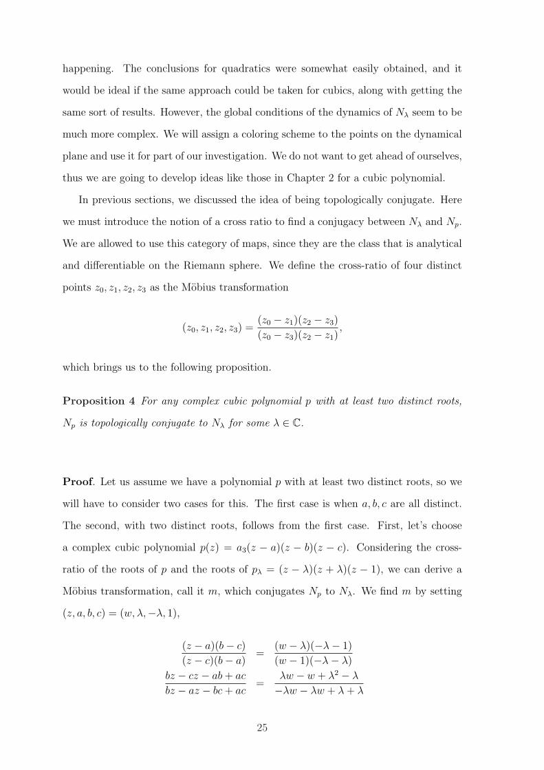
In previous sections, we discussed the idea of being topologically conjugate. Here

we must introduce the notion of a cross ratio to find a conjugacy between Nλ and Np.

We are allowed to use this category of maps, since they are the class that is analytical

and differentiable on the Riemann sphere. We define the cross-ratio of four distinct

points z0, z1, z2, z3 as the Mobius transformation

(z0, z1, z2, z3) =(z0 − z1)(z2 − z3)

(z0 − z3)(z2 − z1),

which brings us to the following proposition.

Proposition 4 For any complex cubic polynomial p with at least two distinct roots,

Np is topologically conjugate to Nλ for some λ ∈ C.

Proof. Let us assume we have a polynomial p with at least two distinct roots, so we

will have to consider two cases for this. The first case is when a, b, c are all distinct.

The second, with two distinct roots, follows from the first case. First, let’s choose

a complex cubic polynomial p(z) = a3(z − a)(z − b)(z − c). Considering the cross-

ratio of the roots of p and the roots of pλ = (z − λ)(z + λ)(z − 1), we can derive a

Mobius transformation, call it m, which conjugates Np to Nλ. We find m by setting

(z, a, b, c) = (w, λ,−λ, 1),

(z − a)(b− c)

(z − c)(b− a)=

(w − λ)(−λ− 1)

(w − 1)(−λ− λ)

bz − cz − ab + ac

bz − az − bc + ac=

λw − w + λ2 − λ

−λw − λw + λ + λ

25

(b− c)z + (ac− ab)

(b− a)z + (ac− bc)=

(λ− 1)w + (λ2 − λ)

(−2λ)w + (2λ).

Cross multiplying and solving for w yields

w = m(z) =a1z + b1

c1z + d1

where

a1 = λ(b− 2c + aλ + a− bλ)

b1 = λ(−2ab + ac− acλ + bcλ + bc)

c1 = bλ− 2cλ + aλ + a− b

d1 = −2abλ + acλ− ac + bcλ + bc.

This is somewhat tedious to work with, so let’s simplify by finding a value of λ for

which the map m is an affine map. That is, make the function a linear mapping. We

set c1 = 0 we get the following transformation

m(z) =a1

d1

z +b1

d1

,

and solve for λ to give us

λ =a− b

2c− (a + b).

Now, if we substitute this value of λ, we get the affine transformation m(z) = Az + B

where

A =2

2c− (a + b)and B = − a + b

2c− (a + b)

In this case, we need 2c 6= a + b, then m sends a → λ, b → −λ, and c → 1. It

immediately follows that Np ∼ Nλ where

p(z) = k(pλ m)(z) = 8k(z − a)(z − b)(z − c)

(2c− (a + b))3

26

and k is the constant a3(2c−(a+b))3

8. This is topological conjugacy and is easily verified

by calculating

Np(z) = m−1 Nλ m(z) =2z3 − cz2 − bz2 − az2 + abc

3z2 − 2az − 2bz − 2cz + ab + bc + ca. (3.1)

Here we find m−1(z) by simply using m(z) and obtaining m−1(z) = (c− a−b2

)z + a+b2

.

In the case where 2c = a + b, we have c = a+b+c3

as a critical point of Np. The critical

point for Nλ is 13, the average of the roots of pλ. Since c → 1, our transformation

m cannot be a conjugacy between Np and Nλ. Our conjugacy must send the critical

point of Np to the critical point of Nλ. Now, if we solve either the transformations

(z, a+b2

, a, b) = (w, 13,−1

3, 1) or (z, a+b

2, b, a) = (w, 1

3,−1

3, 1) for w, we will have the map

we so desire. In fact, w = m(z) = 3a+b−4z3(a−b)

where equation (3.1) holds for λ = 13.

Now, for the second case, let p have only two distinct roots, a and b. By letting

c = a in our original equation for c1, our map reduces to m(z) = 2z−(a+b)a−b

. This sends

the point a to 1 and b to -1. If we choose λ = ±1, m will conjugate Np to N±1 where

p = a3(z − a)2(z − b). ¤

The cross ratio produces a transformation that depends on the order of the points

z1, z2, z3. So, we can find all the possible conjugacies between Np and Nλ simply by

considering the set of all permutations of the set A = a, b, c which contains the roots of

Nλ. We would solve (z, zi, zj, zk) = (w, λ,−λ, 1) for w which will represent a Mobius

transformation such that w : zi → a, zj → b, zk → c. We will do this for each element

zi, zj, zk in the set of permutations of A.

As for the case where p has only two distinct roots, we have

ma(z) =z − a

b− aand mb(z) =

z − b

a− b

for pa(z) = a3(z−a)2(z−b) and pb(z) = a3(z−a)(z−b)2, respectively. These conjugate

27

Np to Nλ for λ = 1. Also,

m1(z) =2z

a + b− a + b

a− band m2(z) =

−2z

a + b+

a + b

a− b

conjugate Np to N1. These m’s corresponding to p1(z) = (z − a)2(z − b) and p2(z) =

(z − a)(z − b)2, respectively.

If we have a cubic polynomial with three distinct roots, we will have to consider

two cases. The first is where any one root is the average of the other two. In this case,

we have the following conjugating maps

m1(z) =4z

3(b− c)− b + 3c

3(b− c)and m2(z) =

−4z

3(b− c)+

3b + c

3(b− c)for a = b+c

2,

m3(z) =4z

3(a− c)− 3a + c

3(a− c)and m4(z) =

−4z

3(a− c)+

3a + c

3(a− c)for b = a+c

2,

m5(z) =4z

3(a + b)− a + 3b

3(a− b)and m6(z) =

−4z

3(a− b)+

3a + b

3(a− b)for c = a+b

2.

These conjugate Np to Nλ where λ = ±13

since p 13

= p− 13.

On the other hand, for any cubic polynomial p having three distinct roots in which

no one root is the average of the other two, there are three conjugating maps with six

distinct values of λ that conjugate Np to Nλ. These conjugacies are

m1(z) =2z

2c− (a + b)− a + b

2c− (a + b)where 2c 6= a + b

m2(z) =2z

2c− (b + c)− a + b

2c− (b + c)where 2c 6= b + c

m3(z) =2z

2c− (a + c)− a + c

2c− (a + c)where 2c 6= a + c

with corresponding λ values

λ1 =a− b

2c− (a + b), λ2 =

b− c

2a− (b + c), λ3 =

a− c

2b− (a + c).

At this point, let us recall the simple roots of the quadratic f(z) = az2 + bz + d

28

are in fact the two superattractive fixed points of the rational function of degree two

Nf =az2 − d

2az + b.

Also, we have seen that the simple roots of the cubic polynomial

p(z) = 8k(z − a)(z − b)(z − c)

(2c− (a + b))3

are indeed the three superattractive fixed points of the rational function of degree

three

Np(z) =2z3 − cz2 − bz2 − az2 + abc

3z2 − 2az − 2bz − 2cz + ab + bc + ca.

We now come to the following proposition.

Proposition 5 If R is a rational function of degree n with exactly n distinct superat-

tractive fixed points, then R ∼ Np for an nth-degree polynomial p.

Proof. First, let us define R : C → C, where R(z) = z − p(z)q(z)

and p and q share no

common factors. Also, let ρi ∈ C for i = 1, 2, ..., n be the n distinct superattractive

fixed points of R. If ρi is fixed for R then, p(ρi)q(ρi

= 0. We know, since ρi is a root of our

polynomial p, that (z−ρi) divides p for i = 1, 2, ..., n. Also, since ρi is a superattractive

fixed point for R, then R′(ρi) = 0. Given that R

′= 1− qp

′−pq′

q2 = q2−qp′+pq

′

q2 , this tells

us that (z−ρi) divides q2−qp′+pq

′. Furthermore, since we know that (z−ρi) divides

p, and thus divides pq′, we also know that it divides q2 − qp

′+ pq

′ − pq′= q(q − p′).

Moreover, p and q have no common factors and (z − ρi) divides p, so (z − ρi) divides

(q − p′) which implies that p

′(ρi) = q(ρi) for i = 1, 2, ..., n.

We know from assumption that the deg(R) = n. Starting with this fact we get the

following implications

deg(R) = n =⇒

deg(zq − p) = n =⇒

29

deg(q) ≤ n =⇒

deg(zq) ≤ n + 1 =⇒

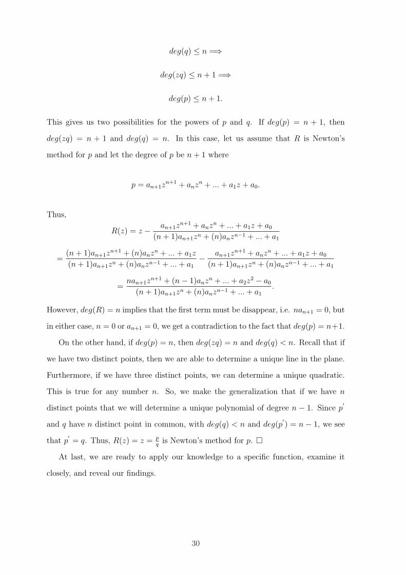
deg(p) ≤ n + 1.

This gives us two possibilities for the powers of p and q. If deg(p) = n + 1, then

deg(zq) = n + 1 and deg(q) = n. In this case, let us assume that R is Newton’s

method for p and let the degree of p be n + 1 where

p = an+1zn+1 + anz

n + ... + a1z + a0.

Thus,

R(z) = z − an+1zn+1 + anzn + ... + a1z + a0

(n + 1)an+1zn + (n)anzn−1 + ... + a1

=(n + 1)an+1z

n+1 + (n)anzn + ... + a1z

(n + 1)an+1zn + (n)anzn−1 + ... + a1

− an+1zn+1 + anzn + ... + a1z + a0

(n + 1)an+1zn + (n)anzn−1 + ... + a1

=nan+1z

n+1 + (n− 1)anzn + ... + a2z2 − a0

(n + 1)an+1zn + (n)anzn−1 + ... + a1

.

However, deg(R) = n implies that the first term must be disappear, i.e. nan+1 = 0, but

in either case, n = 0 or an+1 = 0, we get a contradiction to the fact that deg(p) = n+1.

On the other hand, if deg(p) = n, then deg(zq) = n and deg(q) < n. Recall that if

we have two distinct points, then we are able to determine a unique line in the plane.

Furthermore, if we have three distinct points, we can determine a unique quadratic.

This is true for any number n. So, we make the generalization that if we have n

distinct points that we will determine a unique polynomial of degree n − 1. Since p′

and q have n distinct point in common, with deg(q) < n and deg(p′) = n− 1, we see

that p′= q. Thus, R(z) = z = p

qis Newton’s method for p. ¤

At last, we are ready to apply our knowledge to a specific function, examine it

closely, and reveal our findings.

30

Chapter 4

Graphical Analysis

4.1 The Symmetry of Nλ

Before we dive into our discussion of Nλ, let us first define a triangle created by the

roots of Nλ when λ ∈ C−R. We will denote this triangle Tλ, where each side of Tλ is

determined by any pair of distinct roots. Note that if λ ∈ R, then all the roots will lie

on the real axis and thus will be collinear. We will be able to infer some things about

Nλ just by looking at this triangle. We can even generalize the following property to

generic cubic polynomials.

Proposition 6 If p and q are cubic polynomials whose roots form similar triangles Tp

and Tq, respectively, then Np is conjugate to Nq via some affine map.

Proof. For this proof, we will need to recall a theorem from complex analysis which

states any Mobius transformation can be represented as the composition of a finite

number of inversions, created by the function v(z) = 1z, magnifications, created by the

function m(z) = Az where A ∈ R+, rotations, created by the function r(z) = eiθz

where θ ∈ R, and translations, created by the function t(z) = z + B where B ∈ C.

Consider the geometric representation of the two triangles Tp and Tq. We only need

to make three manipulations to achieve our goal. Recall a linear transformation is of

31

the form

g(z) = az + b, where a, b ∈ C and a 6= 0.

Now, let us consider

g(z) = (m r t)(z)

= m(r(z + c)

= m(eiθ(z + c))

= A(eiθ(z + c))

= Aeiθz + A(eiθc)

= A1z + B1

where A1 = Aeiθ and B1 = Aeiθc. Each of these mappings are non-fractional, linear

mappings, thus g(z) is conformal for all points in the complex plane. With a few

calculations, one can see that the angles of Tp are preserved under each mapping. This

is independent from our choice of c, θ, and A. Therefore, we can choose these such

that g will conjugate Tp to Tq. Thus implying that p conjugates to q, and from our

previous knowledge, making Np conjugate to Nq through this affine map. ¤

The following pictures illustrates the rate of convergence for each point in the plane

with a different color. We can see that the points form a right triangle in the plane.

Thus, any roots from another polynomial that form a right triangle will be conjugate

to this polynomial.

32

Figure 4.1: Newton’s method on the cubic polynomial p(z) = z3 + z2 + z + 1. Here, λ= i.

Not only can the function created with the Newton’s method of our particular

family of cubic polynomials be examined by the triangles created with the roots, even

when we do not see a triangle, Nλ exhibits some very nice properties. In fact, what

we realize is that the roots of the triangle have become collinear and form a line the

plane.

This exemplifies the following proposition.

Proposition 7 If λ ∈ R, then Nλ is symmetric with respect to the real axis.

Proof. For this proof, all we need to show is that for the two complex roots of the

function

Re(Na(z)) = Re(Na(z)) and Im(Na(z)) = Im(Na(z))

Re(Na(a + bi) = Re(Na(a− bi)) and Im(Na(a + bi)) = −Im(Na(a− bi)).

In this case, we call our function Na since we are assuming that we have λ ∈ R. Refer

back to our original Newton function,

Nλ =2z3 − z2 − λ2

3z2 − 2z − λ2,

33

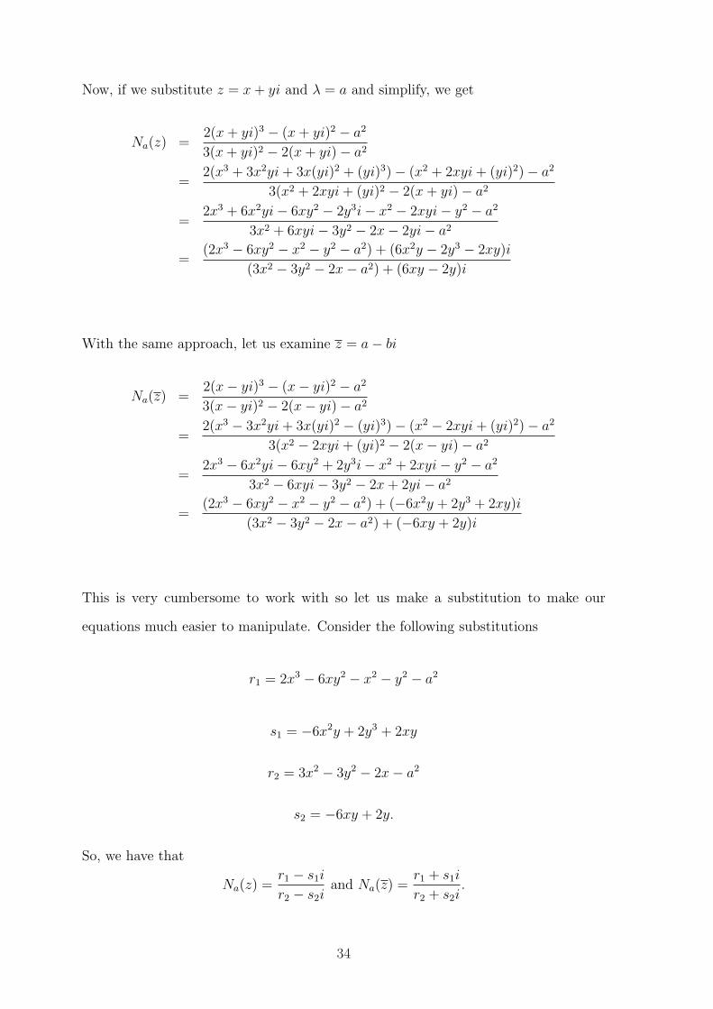
Now, if we substitute z = x + yi and λ = a and simplify, we get

Na(z) =2(x + yi)3 − (x + yi)2 − a2

3(x + yi)2 − 2(x + yi)− a2

=2(x3 + 3x2yi + 3x(yi)2 + (yi)3)− (x2 + 2xyi + (yi)2)− a2

3(x2 + 2xyi + (yi)2 − 2(x + yi)− a2

=2x3 + 6x2yi− 6xy2 − 2y3i− x2 − 2xyi− y2 − a2

3x2 + 6xyi− 3y2 − 2x− 2yi− a2

=(2x3 − 6xy2 − x2 − y2 − a2) + (6x2y − 2y3 − 2xy)i

(3x2 − 3y2 − 2x− a2) + (6xy − 2y)i

With the same approach, let us examine z = a− bi

Na(z) =2(x− yi)3 − (x− yi)2 − a2

3(x− yi)2 − 2(x− yi)− a2

=2(x3 − 3x2yi + 3x(yi)2 − (yi)3)− (x2 − 2xyi + (yi)2)− a2

3(x2 − 2xyi + (yi)2 − 2(x− yi)− a2

=2x3 − 6x2yi− 6xy2 + 2y3i− x2 + 2xyi− y2 − a2

3x2 − 6xyi− 3y2 − 2x + 2yi− a2

=(2x3 − 6xy2 − x2 − y2 − a2) + (−6x2y + 2y3 + 2xy)i

(3x2 − 3y2 − 2x− a2) + (−6xy + 2y)i

This is very cumbersome to work with so let us make a substitution to make our

equations much easier to manipulate. Consider the following substitutions

r1 = 2x3 − 6xy2 − x2 − y2 − a2

s1 = −6x2y + 2y3 + 2xy

r2 = 3x2 − 3y2 − 2x− a2

s2 = −6xy + 2y.

So, we have that

Na(z) =r1 − s1i

r2 − s2iand Na(z) =

r1 + s1i

r2 + s2i.

34

Multiplying the top and bottom by the complex conjugate of each denominator, we

achieve

Na(z) =r1r2 + s1s2

r22 + s2

2

+(−r2s1 + r1s2)

r22 + s2

2

i

Na(z) =r1r2 + s1s2

r22 + s2

2

+(r2s1 − r1s2)

r22 + s2

2

i

With this representation it is easy to see that the real parts of Na(z) and Na(z) are in

fact equal, and the corresponding imaginary parts are complex conjugates. ¤

Back to the feature of Nλ that we have discussed about the appearance of a triangle

created from the roots of pλ when λ ∈ C−R. We viewed this triangle before in Figure

3.2. We have the following proposition in which Tλ tells us something about Nλ.

Proposition 8 If Tλ is an isosceles triangle, then Nλ is symmetric with respect to the

line determined by the median of Tλ which divides Tλ into two equal parts.

Proof. If we have an isosceles triangle, then we can say that any point in the plane z0 is

of equal distance from exactly two roots of the polynomial. For this, we must consider

the following three cases of an isosceles triangle Tλ, 1) |λ−z0| = |−λ−z0|, 2) |1−z0| =|λ− z0|, and 3) |1− z0| = | − λ− z0|.

Let us begin with case one. Well, we start with λ = a + bi and see that

|λ− z0| = | − λ− z0|√(a− 1

3)2 + b2 =

√(−a− 1

3)2 + b2

(a− 1

3)2 + b2 = (−a− 1

3)2 + b2

a− 1

3= ±(a +

1

3)

This gives us the two equations a − 13

= a + 13

and a − 13

= −a − 13. Thus, a = 0

and b ∈ R. Here, we find that λ = bi lies along the imaginary axis, and the real axis

contains the median that divides the two equal sides of Tλ. So, this comes down to

35

showing in the same manner as in Proposition 7 that

Re(Nbi) = Re(Nbi(z)) and Im(Nbi(z)) = Im(Nbi(z)).

In fact, we have

Nbi(z) =(2x3 − 6xy2 − x2 + y2 + b2) + (6x2y + 2y3 + 2xy)i

(3x2 − 3y2 − 2x + b2) + (6xy − 2y)i

and

Nbi(z) =(2x3 − 6xy2 − x2 + y2 + b2) + (−6x2y + 2y3 + 2xy)i

(3x2 − 3y2 − 2x + b2) + (−6xy + 2y)i

which satisfy the given equations, because they are complex conjugates.

Now, look at case two. Again, let us start with

|1− z0| = |λ− z0|√(1− 1

3)2 + 02 =

√(a− 1

3)2 + b2

(2

3)2 = (a− 1

3)2 + b2

What we have now is the equation for a circle centered at the point (13, 0) with

radius 23. For each λ not on the real or imaginary axis, there exist two distinct values

of γ such that Re(γ) = 0 and Tλ is similar to Tγ. This follows from the fact that we

have six distinct values of λ which are conjugate to each other and three distinct sets

whose members represent λ values for which one root is equidistant to any other two.

These three sets consist of two circles centered at 13

and −13

both with radius 23. Thus,

by proposition 6, Nλ conjugate to Nγ. Since γ lies on the imaginary axis, we have

by proposition 7 that Nγ is symmetric with respect to the real axis. Therefore, Nλ is

symmetric with respect to the median of Tλ which divides the triangle into two equal

parts.

36

Finally, we look at case three where

|1− z0| = | − λ− z0|√(1− 1

3)2 + 02 =

√(a +

1

3)2 + b2

(2

3)2 = (a +

1

3)2 + b2

This case is analogous to case 2. There are corresponding distinct values of γ along the

imaginary axis such that Nλ is conjugate to Nγ where Nγ is symmetric with respect

to the real axis. Therefore, Nλ is symmetric with respect to the median of Tλ into two

congruent triangles. ¤

What other types of triangles are there? Perhaps a more interesting question would

be “do other types of triangles imply something about the Newton function to which

they correspond?” As a matter of fact, there are other implications to be made.

Proposition 9 If Tλ is an equilateral triangle then Nλ is symmetric with respect to

each median of Tλ.

Proof. Solving the equation z = 1, we get the cube roots of unity. Define µ : z → z3−1

and calculate

Nµ(z) = z − z3 − 1

3z2=

2z3 + 1

3z2.

It is easily verified that for A(z) = ze23πi

Nµ(z) = A Nµ A−1(z).

We then can apply proposition 6, the proposition that states if two cubics have similar

triangles, then their Newton functions are conjugate to each other. Hence, Nλ is

symmetric about each median of Tλ. ¤

We also have triangles that are scalene.

37

Proposition 10 If Tλ is scalene, then Nλ is not symmetric with respect to any line

in the plane.

Proof. Let us start with a line l in the plane. Also, let us assume that the roots of pλ

are distinct and form a triangle Tλ. We want to see that the line l will separate the

plane into two distinct hemispheres which do not contain the same number of roots, in

other words, are not symmetric. Consider on the hemisphere with the greater number

of roots. We can find a point p ∈ l that is not a root of pλ such that p and one of

the roots r are equidistant to any particular point on l. However, Nλ(r) is a fixed

point of Nλ and Nλ(p) is a not fixed point of Nλ. Thus, they cannot be equidistant to

any point in l. In this case, the only way that symmetry will occur is if we have the

situation where the line l splits the plane into two hemispheres that contain exactly

one root. Let k be the line determined by the roots of pλ which are not in l. If l does

not intersect k orthogonally then for each root r ∈ k there exists a point r′

not in

k such that r′and r are equidistant to any point in l, but Nλ(r) and Nλ(r

′) are not

equidistant to any point in l. If l intersects k orthogonally then l does not intersect

the midpoint of the line segment determined by the roots in k since Tλ is scalene. So

the two roots in k are not equidistant to any point in l. This means for each r ∈ k

there exists a point r′ ∈ k which is not a root of pλ such that r and r

′are equidistant

to any point in l, but Nλ(r) and Nλ(r′) are not equidistant to any point in l. ¤

Now, let us dive into a closer examination of Nλ.

4.2 Newton’s Method for Cubic Polynomial Nλ

In Chapter 3, we proved that any complex cubic polynomial with at least two distinct

roots is topologically conjugate to

Nλ =2z3 − z2 − λ2

3z2 − 2z − λ2

38

where λ = a−b2c−(a+b)

is the only parameter with a, b, c as the coefficients of our cubic

polynomial. We have also discovered the graphical representation of the behavior of

quadratic polynomials in Chapter 2. This Newton function, Nλ, is that in which we

will be referring to for the remainder of the discussion. We want to utilize the ability of

computer graphics created with the program MatLab which will enable us to describe

and visualize the dynamics of cubic polynomials.

Recall from Chapter 3 the proof of Proposition 4. We found in our calculations

that there is an extra critical point for z = 13. It is this extra critical point that allows

us to view the parameter space where we plot Nλ(13) for each value of λ. Since we

have already chosen our function, the question that naturally follows is “what is the

behavior of Nλ for different values of λ?”

Unlike the spaces created with a rainbow coloring, which simply indicate the rate

of convergence for points, we will color the parameter space with only three colors.

Each color will correspond to the root to which that point is attracted. A picture of

the space created with these criteria is shown in figure 4.1.

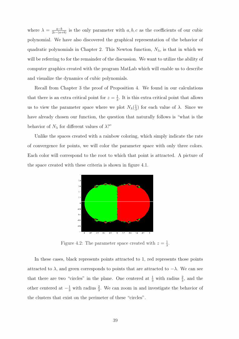
Figure 4.2: The parameter space created with z = 13.

In these cases, black represents points attracted to 1, red represents those points

attracted to λ, and green corresponds to points that are attracted to −λ. We can see

that there are two “circles” in the plane. One centered at 13

with radius 23, and the

other centered at −13

with radius 23. We can zoom in and investigate the behavior of

the clusters that exist on the perimeter of these “circles”.

39

Figure 4.3: Excerpt from parameter space figure.

In this figure, we have a new color that we did not see before we zoomed in on the

figure. Let us again zoom in to examine closely the shape of this area.

Figure 4.4: The set of periodic points from our parameter space.

From previous experience, we know that the shape of this figure is that of the

Mandlebrot set. This raises the question: “How do the points that are colored yellow

behave?”

Now, to investigate this question about Nλ, let us focus on the behavior of a

particular point in the plane. The Julia set of a complex function is the set of all

points on the boundary between the set of points that escape to infinity and the set

of points that do not escape to infinity. We see this with the following example.

Consider the value λ = .589 + .605i. This is a value located in the Mandelbrot set

of our parameter space. Let’s look at the convergence of all the points under Newton’s

method. We see this illustration is Figure 4.5.

40

Figure 4.5: Nλ for λ = .589 + 605i from -1.5 to 1.5.

Now, we zoom in on the portion in the center that looks like it is glowing. As we

zoom in, we see this part taking shape. It looks like a rabbit. This is our Julia set for

the particular polynomial created with λ = .589 + .605i.

Figure 4.6: Nλ for λ = .589 + .605i from 0 to 1.5.

The rabbit is not the only figure that we can see with a particular value of λ.

We also gets pictures that illustrate parts of nature like elephants, spiders, and many

more.

41

Figure 4.7: “The Rabbit”: Nλ for λ = .589 + .605i from 0.2 to .48.

We have accomplished our goal of viewing the dynamics of cubic polynomials after

the iterations of Newton’s method. The graphical nature of the iterations gave us very

nice properties that allow us to describe the behavior of the points in the plane. This

leads us to ponder a question about repeating the same investigation with higher degree

polynomials. Following these investigations, would we be able to make assumptions

and develop theory for polynomials of nth degree? In the future, this is a question

that deserves some attention.

42

Appendix A

MatLab Code

A.1 Newton’s Method on Quadratic Polynomials

%Shannon Miller

%Marshall University

%2006

%This program will plot convergence of the values for the Newton

%function of a quadratic polynomial with a particular coefficients.

%Simply change the values for the min and max of the x axis and y

%axis to zoom in and/or out. Figures 2.1 and 2.2 with

%lambda = .589 +.605i.

function NMQ(a,b,c)

% default setting

if (nargin < 7)

min_re = -5;

max_re = 5;

min_im = -5;

max_im = 5;

43

n_re = 500;

n_im = 500;

tol = 0.01;

end

coeff = [a b c];

polyRoots = roots(coeff)

format compact;

max_steps = 10;

% stepsize

delta_re = (max_re-min_re)/n_re; delta_im = (max_im-min_im)/n_im;

x = min_re:delta_re:max_re; y = min_im:delta_im:max_im;

[X,Y] =

meshgrid(x,y); Z = X + i*Y;

for j = 1:n_im + 1

for k = 1:n_re + 1 % one pixel z = (j,k)

z = Z(j,k);

if z == 0

z = tol;

end

m = 0;

flag = 0;

while (flag == 0)

% iteration

z = z - (a*z.^2 + b*z + c)./(2*a*z + b);

if norm(a*z.^2 +b*z +c) <= tol

% we are next to a zero

flag = 1;

end

44

if m > max_steps

flag = 1;

end

m = m + 1;

end

% assign color according to number of steps

Z(j,k) = m;

end

end

% plot the result

%colormap(hot);

colormap(prism(10)); brighten(0.5);

%image(Z)

pcolor(X,Y,Z)

%axis off;

shading flat;

A.2 Newton’s Method on Cubic Polynomials

%Shannon Miller

%Marshall University

%2006

%This program will plot convergence of the values for the Newton

%function of a cubic polynomial for any choice of coefficients.

%Simply change the values for the min and max of the x axis and y

%axis to zoom in and/or out. Figure 4.1 illustrates.

function NMC(a,b,c,d)

45

% default settings

min_re = -1.5;

max_re = 1.5;

min_im = -1.5;

max_im = 1.5;

n_re = 300;

n_im = 300;

tol = 0.01;

coeff = [a b c d]; polyRoots = roots(coeff)

format compact;

max_steps = 20;

% stepsize

delta_re = (max_re-min_re)/n_re; delta_im = (max_im-min_im)/n_im;

x = min_re:delta_re:max_re; y = min_im:delta_im:max_im;

[X,Y]=meshgrid(x,y); Z = X + i*Y;

for j = 1:n_im + 1

for k = 1:n_re + 1 % one pixel z = (k,j)

z = Z(j,k);

if z == 0

z = tol;

end

m = 0;

flag = 0;

while (flag == 0)

% iteration

z = z - (a*z.^3 + b*z.^2 + c*z +d)./(3*a*z.^2 + 2*b*z + c);

if norm(a*z.^3 + b*z.^2 + c*z +d) <= tol

% we are next to a zero

46

flag = 1;

end

if m > max_steps

flag = 1;

end

m = m + 1;

end

% assign colour according to number of steps

Z(j,k) = m;

end

end

% plot the result

colormap(hot);

%colormap(prism(20));

brighten(0.5);

%image(Z)

pcolor(X,Y,Z)

%axis off;

shading flat;

A.3 Newton’s Method on Lambda Cubic

%Shannon Miller

%Marshall University

%2006

%This program will plot the rate convergence for values of the Newton

%function of a cubic polynomial with a particular value of lambda.

%Simply change the values for the min and max of the x axis and y

%axis to zoom in and/or out. Figures 4.5, 4.6 and 4.7 with

47

%lambda = .589 +.605i.

function NMNLambda(lambda)

% default setting

if (nargin < 7)

min_re = 1.5;

max_re = 1.5;

min_im = -1.5;

max_im = 1.5;

n_re = 200;

n_im = 200;

tol = 0.01;

end

%forms x and y vectors of n points between min and max default values

x = linspace(min_re, max_re, n_re); y = linspace(min_im, max_im,

n_im);

format compact;

max_steps = 50;

% stepsize

[X,Y] = meshgrid(x,y); Z = X + i*Y;

for j = 1:n_im

for k = 1:n_re % one pixel z = (k,j)

z = Z(j,k);

if z == 0

z = tol;

end

m = 0;

flag = 0;

48

while (flag == 0)

% iteration

z = z - (z.^3 - z.^2 - (lambda.^2)*z + lambda.^2)./

(3*z.^2 - 2*z - lambda.^2);

if norm(z.^3 - z.^2 - (lambda^2)*z + lambda^2) <= tol

% we are next to a zero

flag = 1;

end

if m > max_steps

flag = 1;

end

m = m + 1;

end

% assign colour according to number of steps

Z(j,k) = m;

end

end

% plot the result

%colormap(hot);

colormap(jet(50)); brighten(0.5);

%image(Z)

pcolor(X,Y,Z)

%axis off;

shading flat;

A.4 Parameterspace

%Shannon Miller

%Marshall University

%2006

49

%This program will plot the convergence of z = 1/3 for a particular

%value of lambda. Simply change the values for the min and max of the

%x axis and y axis to zoom in and/or out. Figures 4.1, 4.2 and 4.3

%show this.

function parameterspaceTest(iter)

% default setting

min_re = 1.3;

max_re = -1.3;

min_im = 1;

max_im = -1;

n_re = 500;

n_im = 500;

tol = 0.0001;

format compact;

%forms x and y vectors of 300 points between min and max default values

x = linspace(min_re, max_re, n_re); y = linspace(min_im, max_im,

n_im);

%forms n_re x n_im matrix of x + iy values

[X,Y] = meshgrid(x,y); Lambda = X + i*Y; z = ones(n_re);

z=z*(1/3);

for m = 1:iter

z = z - (z.^3 - z.^2 - Lambda.^2.*z +

Lambda.^2)./(3*z.^2 - 2*z - Lambda.^2); end

green = abs(z - Lambda) < tol;

50

green = green*6;

red=abs(z+Lambda)<tol;

red = red*9;

black = abs(z - 1) < tol;

black = black*13; colors = zeros(n_re) + green + red + black;

yellow = colors == 0; colors = colors + yellow; colors(1, :) = 16;

%set the color map

colormap(hsv); brighten(0.5);

%Map the Lambda matrix to the color map

pcolor(X,Y,colors) shading flat;

51

Bibliography

[1] Blanchard, Paul.,“Complex Analytic Dynamics on the Riemann Sphere,”

Bulletin of the American Mathematical Society, Vol. 11 (1984), 85–144.

[2] Carleson, Lennart and Gamelin, Theodore W., Complex Dynamics, Springer-

Verlag , 2005.

[3] Devaney, Robert L., An Introduction to Chaotic Dynamical Systems, 2nd ed.,

Westview Press, 2003.

[4] Devaney, Robert L., Chaos, Fractals, and Dynamics: Computer Experiments

in Mathematics, Addison-Wesley Publishing Co., 1990.

[5] Gilbert, William J., “Generalizations of Newton’s Method,” Fractals, Vol.

9, No. 3, (2001), 251–262.

[6] Hubbard, J., Schleicher, D., and Sutherland, S., “How to find all roots of

complex polynomials by Newton’s Method,” Inventiones mathematicae, Vol.

146 (2003), 1–33.

[7] Lynch, Stephen, Dynamical Systems with Applications Using MatLab,

Birkhauser, 2004.

[8] Milnor, John, Dynamics in One Complex Variable, F. Vieweg and Sohn,

1999.

[9] Peitgen, H., Jurgens, H., and Saupe, D., Chaos and Fractals: New Frontiers

of Science, Springer-Verlag, 1992.

52

[10] Roberts, Gareth E. and Horgan-Kobelski, Jeremy, “Newton’s versus Hay-

ley’s Method: A Dynamical Systems Approach,” International Journal of

Bifurcation and Chaos, Vol. 14 No. 10, (2004), 3459-3475.

[11] Saff, E. B., and Snider, A. D., Fundamentals of Complex Analysis for Math-

ematics, Science, and Engineering, Prentice-Hall, Inc., 1976.

53