the dynamics of marriage and divorce - iza institute of ...ftp.iza.org/dp6379.pdfthe dynamics of...

DI

SC

US

SI

ON

P

AP

ER

S

ER

IE

S

Forschungsinstitut zur Zukunft der ArbeitInstitute for the Study of Labor

The Dynamics of Marriage and Divorce

IZA DP No. 6379

February 2012

Gustaf BruzeMichael SvarerYoram Weiss

The Dynamics of Marriage and Divorce

Gustaf Bruze Aarhus University

Michael Svarer

Aarhus University and IZA

Yoram Weiss Aarhus University,

Tel Aviv University and IZA

Discussion Paper No. 6379 February 2012

IZA

P.O. Box 7240 53072 Bonn

Germany

Phone: +49-228-3894-0 Fax: +49-228-3894-180

E-mail: [email protected]

Any opinions expressed here are those of the author(s) and not those of IZA. Research published in this series may include views on policy, but the institute itself takes no institutional policy positions. The Institute for the Study of Labor (IZA) in Bonn is a local and virtual international research center and a place of communication between science, politics and business. IZA is an independent nonprofit organization supported by Deutsche Post Foundation. The center is associated with the University of Bonn and offers a stimulating research environment through its international network, workshops and conferences, data service, project support, research visits and doctoral program. IZA engages in (i) original and internationally competitive research in all fields of labor economics, (ii) development of policy concepts, and (iii) dissemination of research results and concepts to the interested public. IZA Discussion Papers often represent preliminary work and are circulated to encourage discussion. Citation of such a paper should account for its provisional character. A revised version may be available directly from the author.

mailto:[email protected]

IZA Discussion Paper No. 6379 February 2012

ABSTRACT

The Dynamics of Marriage and Divorce* We formulate and estimate a dynamic model of marriage, divorce, and remarriage using 27 years of panel data for the entire Danish cohort born in 1960. The marital surplus is identified from the probability of divorce, and the surplus shares of husbands and wives from their willingness to enter marriage. Education and marriage order are complements in generating gains from marriage. Educated men and women receive a larger share of the marital gains but this effect is mitigated when their proportion rises. Education stabilizes marriage and second marriages are less stable. As the cohort ages, uneducated men are the most likely to be single. JEL Classification: J12 Keywords: marriage, divorce, sorting Corresponding author: Michael Svarer School of Economics and Management Aarhus University 8000 Aarhus C Denmark E-mail: [email protected]

* We thank the Danish Social Science Research Foundation, The Danish Council for Independent Research in Social Sciences, and the Cycles, Adjustment, and Policy Research Unit (CAP) at Aarhus University for financial support. We also thank Rune Vammen Lesner and Jonas Maibom Pedersen for excellent research assistance. Finally, we thank Jerome Adda, B J Christensen, John Knowles, Dale Mortensen, Victor Rios-Rull, and Aloysius Siow for useful comments on previous drafts.

mailto:[email protected]

1 Introduction

Modern marriage markets are characterized by high turnover; men and women divorce

more but also remarry more than in the past. However, di¤erent individuals have di¤erent

marital histories; they marry, divorce, and remarry at di¤erent rates. To explain this

variation it is crucial to understand the two-sided aspect of marriage markets. Marriages

form and dissolve based on preferences and expectations of two di¤erent individuals who

operate in a "marriage market" with many competing agents.

In this paper, we examine the marriage patterns within a large cohort consisting of

all men and women in Denmark who were born in 1960, which we observe from age 20

to age 46. We have information not only on their own attributes and marital history

but also on that of their various spouses. The spouses can belong to di¤erent cohorts

and thus may be younger or older than the respondents. We consider two alternative

de�nitions of marriage: legal marriages and partnerships that include legal marriages and

cohabitation. Most initial partnerships involve cohabitation but upon approaching age 46

most partnerships are marriages. The hazards of entry into and exit out of partnerships

are initially much larger than the hazards of entry and exit into regular marriage. However

long term partnerships have similar exit and entry rates to legal marriages. We mainly

analyze legal marriages. We then show that, in the long term, the matching patterns are

similar under the two de�nitions.

We focus on marriage patterns by completed education at age 46, when men and

women are classi�ed into three education groups. We then ask which types of individuals

are more likely to marry, to stay married, and to remarry and which types of marriage

(based on the education of both partners) are more stable. We analyze the complex

dynamic interactions between marriage, divorce and assortative matching as they evolve

over time. Assuming that agents are forward-looking such analysis requires a structural

model that speci�es the marital preferences of men and women for di¤erent types, their

expectations of future marital options and the marital choices that they make based on

these expectations. We also need to specify how the marriage market operates in terms of

the meeting technology and the ability of spouses to transfer economic resources between

each other in order to attract partners into marriage and maintain the stability of the

marriage.

We formulate and estimate such a model and show that it �ts the data well. The

general approach is matching without frictions. The basic simplifying assumption is that

2

individuals can be classi�ed into few categories. Every man (woman) is indi¤erent between

all women (men) in the same category but still has idiosyncratic preferences over categories

(meeting one person of each category is su¢ cient). Given a large number of men and

women in each category, the share that each agent receives of the systematic gains from

marriage is the same with all potential spouses of a given category. These common share

components satisfy stability conditions and respond to the number of single men and

women of each type in a given year.

A major challenge for any economic analysis of marriage is that in most cases the

"prices" or the division of marital gains are not observed. The methodological innovation

of this paper lies in the ability to infer such transfers from data in which one observes

both marriage and divorce. Information on the dissolution of marriages of di¤erent types

provides information on the joint value of the marriage to both partners. The willingness of

each single man and woman to enter into a particular type of marriage gives us information

on the gains from marriage that each one of them expects separately. The paper provides

a dynamic analysis of the gains from marriage, its division and the sorting by education

in a given cohort over time. In this regard we extend and complement previous work by

Choo and Siow (2006) and Chiappori, Salanie and Weiss (2011). The panel data that we

use allows us to observe both the in�ows and the out�ows into di¤erent types of marriage,

which provides more information on the gains from marriage and its division than what

can be obtained from cross-section data.

Similar to previous studies, we �nd strong assortative matching by education. A novel

aspect of our data is to show that such sorting operates gradually via the selection into

�rst and second marriages and also by the selection out of these marriages, based on the

education level of both partners. In particular we �nd that men with low education are

increasingly sorted out of marriage and remain or end up single. This happens because

marriages in which both partners or the men have low education dissolve at a higher rate.

Our model captures these basic features by showing that the marital output �ow and the

expected marital surplus is supermodular in the education of the husband and the wife

which implies that the total aggregated marital output �ow over all possible assignments,

is maximized when agents marry a spouse with the same education. Our results also

indicate that education raises the marital output �ow, and that more educated men and

women receive a larger share of the marital surplus. In addition, women receive a lower

share of the marital surplus in second marriage.

A closely related paper is Brien, Lillard and Stern (2006). They estimate a dynamic

3

model of marital transitions for women in the US. They include learning about match

quality, children as an exogenous event, and a three-way choice between singlehood, co-

habitation, and marriage. Our approach complements their work by emphasizing the

two-sided aspects of the marriage problem and the role of competition. A recent paper

by Gemici and Laufer (2011) extends that work to include the di¤erent division of labor

of cohabiting and married couples. Another related paper is Aiyagari et al. (2000) that

construct a dynamic model of marriage and divorce and use calibration to simulate the

impact of policy changes such as child support. Although our data includes information

about children, we do not use that information in this work. Instead, our focus is on

assortative matching by schooling as it evolves over time and the associated shares in the

gains of marriage that partners with di¤erent schooling obtain.

We proceed by �rst describing our unique Danish data in terms of the assignment

patterns by education within a cohort as it ages. We provide details on the transitions

between marriage, divorce and remarriage, separating �rst and second marriages. We then

describe the model and highlight the main assumptions. Finally, we present and discuss

the estimated parameters, the derived marital output �ow, the estimated expected marital

surplus, and the husband�s and wife�s surplus and marital shares.

2 The sample

The data we use is register-based and is collected by Statistics Denmark. All information

is derived from public registers which are combined according to a social security number

(all Danish citizens have a social security number). The data set follows the 1960-cohort

annually from 1980-2006 (i.e. from ages 20 to 46). In order to be included in a given

year, individuals must have an address in Denmark. This implies that individuals who

are not living in Denmark in a given year are not sampled in that year and do not have a

complete marital history. We restrict the sample to individuals with records in all years

which implied that we lost around 24% of the sample (50% of these were immigrants who

were born in 1960 but entered Denmark after 1980). In addition, we eliminated those

who were married at age 20. This additional restriction caused us to lose about 4 percent

of our sample, mainly women. This leaves us with 61780 individuals.

4

2.1 Education groups

We distinguish between three education groups, based on level of completed education at

age 46: high school or less, vocational education, and college (de�ned as some college or

more).

Table 1 below shows the distribution by level of education for men and women. There

is about an equal number of men and women in the sample. However, the distribution by

education di¤ers between men and women. We see that the proportion with high school

or less is slightly higher for men, the proportion with vocational education is also higher

for men but the proportion with some college or more is higher for women.1

TABLE 1

Sample distribution of male and female completed education

Completed Education (at 46) Men Women

High school or less 0.33 0.30

Vocational education 0.41 0.37

Some college or more 0.26 0.33

No. of observations 31835 29945

2.2 Individual Marriage Patterns

2.2.1 Cohabitation and marriage

Cohabitation is a common phenomenon in Denmark (see e.g. Svarer 2004). More than

60% of all young couples are cohabiting and it is somewhat more common among men

and women with a high level of completed education. To be classi�ed as cohabiting by

Statistics Denmark, an individual must share an address with an opposite sex person

who is not family-related, and who is no more than 15 years older or younger than the

individual. This measure is more noisy than legal marriage, since e.g. two students of

opposite sex who share a �at but are not in a relationship will be registered as cohabiting.

1As mentioned, we exclude individuals for which we do not have complete marriage market histories.

The sample attrition tends to sort out the more highly educated from the �nal sample.

5

In this paper we do not try to model the cohabitation decision explicitly but consider two

alternative de�nitions: legal marriages and partnerships that include legal marriages and

cohabitation. A three-state model with cohabitation as a separate choice is left for future

work.2

As one can see in the Figures 1, 2 and 3, most initial partnerships involve cohabitation

but upon approaching age 46 most partnerships are marriages. Also, the hazards of entry

into and exit out of partnerships are initially much larger than the hazards of entry and

exit into regular marriage.

2.2.2 Marriage patterns by education and gender

Figure 4 shows the proportions of men and women in marriage and partnership, respec-

tively, by education. At early ages, women with medium education enter marriage and

partnership at the highest rate. Highly educated men and women delay their entry, but

by age 46 they are the most likely to be married. Men with low education are increas-

ingly left behind and by age 46 about 55% of them are unmarried and 41% are without

a partner. These time patterns are very similar for marriages and partnerships.

2.2.3 Marriage and divorce hazards

The time patterns of the proportions married can be traced back to di¤erences in the

hazard to enter marriage, exit from marriage and to remarry in our sample. Figures 5

and 6 show the hazards of entry and exit into and out of �rst marriages. As one would

expect, the hazard rates into �rst marriage are higher for women at early ages and highly

educated men and women delay their marriage. Divorce hazards are highest in marriages

involving low education agents and lowest when the two partners are highly educated.

Hazards of entry into second marriage are higher than into �rst marriage.

2.2.4 Who marries whom

Conditioned on his/her education, each man (woman) can marry three types of spouses

distinguished by their level of education. The actual choices made depend on gender and

2There are di¤erent legal implications of cohabitation vis-à-vis formal marriage. In some respects,

couples who cohabited for more than two years least two years are considered as married. For instance,

the law stipulates that if a couple has cohabited for more than two years the partner has the right to

keep the apartment if the other partner (who originally rented the apartment) dies.

6

the agent�s own level of education as shown in Figures 9 and 10. We see that highly

educated men marry mainly highly educated women. This proportion rises sharply as the

cohort advances in age and reaches 60% at age 46. The probability for a highly educated

man to have a wife with high school or less declines sharply, reaching 13% at age 46. About

half of the wives of men with vocational education have vocational education themselves

and this proportion remains stable as the cohort ages. Men with low education marry

mainly women with low education. With the passage of time, the proportion of marriages

of low education men with women of higher education rises, re�ecting the higher stability

of these marriages.

The marital choices of women are similar to those of the men with some noticeable dif-

ferences: The proportion of highly educated women that have a highly educated husband

at age 46 is 53%, which is lower than the proportion of highly educated men that have a

highly educated wife, which is 60%. The proportion of highly educated women that have

a husband with low education at age 46 is 16%, which is higher then the proportion of

highly educated men that have a wife with low education which is 13%. These di¤erences

re�ect the fact that women in our sample are more educated than men and, therefore,

forced to marry a husband with less education.

The choice probabilities are similar when we replace marriages by partnerships (i.e.

legal marriage or cohabitation). For instance, conditioned on being in a partnership, the

probability that a highly educated man will be in a partnership with a highly educated

woman is 61%. The corresponding probability for educated women is 49%.

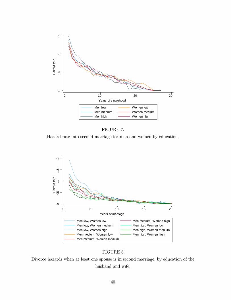
2.2.5 Second marriages

Individuals who divorce remarry quickly and the hazards of entry into second marriage

exceed the hazards of entry into �rst marriage (see Figure 7). This indicates that individ-

uals who divorce wish and are able to remarry rather quickly (see Browning, Chiappori,

and Weiss 2011, chapter 1). Men enter second marriages faster than women, especially

educated men. The time patterns of the marital choices of di¤erent types of agents, con-

ditioned on �rst and second marriages, are also quite close to each other. This is true

for both men and women. Thus, from the point of view of the assignment, it does not

matter much if one is in a second or �rst marriage when one gets beyond age 30 or so.3

However, second marriages are substantially less stable than �rst marriages, especially if

3One exception is that the proportion of marriages in which both partners have medium education is

higher in �rst marriages.

7

both spouses have low education. This is consistent with the �ndings of Svarer (2004)

using Danish data, and the �ndings of Parisi (2008) using British data.

2.2.6 Sorting in the marriage market

As members of the cohort advance in age and make their marriage and divorce decisions

each year, the composition of married couples by the education of the spouses and the

composition of singles by their own education both change. Changes in the degree of

sorting over time occurs mainly through two mechanisms: First, marriages in which both

partners are highly educated are the most stable and, therefore, their proportion among

all marriage rises. Second, men and women with low education are more likely to remain

single following marital dissolution and, therefore, marriages involving individuals with

low education become increasingly rare. This trend is noticeably stronger among men.

By age 46, 54% of the unmarried men have low education compared with the 31% who

have high education. The corresponding percentages among women are 46 % and 36%,

respectively. The role of education in stabilizing marriages and the di¢ culties that less

uneducated men face in marriage are not special to Denmark. Similar results for the US

are reported by Weiss and Willis (1997), Stevenson and Wolfers (2007), and Chiappori,

Salanie, and Weiss (2011).

3 A dynamic model of marriage and divorce

3.1 The general approach

We now propose a dynamic model that captures and interprets the main features observed

in our data. The general approach is matching with transferable utility and without

frictions. Within this framework, the basic simplifying assumption is that individuals can

be classi�ed into few types. Every man (woman) is indi¤erent between all women (men)

of the same type but still has idiosyncratic preferences over types. Given a large number

of men and women in each type, the share that each agent receives of the systematic

gains from marriage is the same for all members of a given type. These common shares

are determined by stability conditions and generally respond to market conditions. When

making choices, individuals anticipate the aggregate e¤ects that are transmitted through

the shares of the marital surplus that husbands and wives receive each year during their

lifetime. In this framework, we analyze individual choices to marry, divorce, and remarry.

8

We also analyze aggregate outcomes such as the number of men and women that remain

single, the types of marriage that are formed and survive, and the educational composition

of di¤erent marital groups over time.

3.2 Types of Men and Women

Time is discrete and the economy is populated by men and women who can choose to be

single or marry a member of the opposite sex. All men and women live for T periods, die,

and then receive no further utility. Utility �ows over these T time periods are discounted

geometrically with the discount factor R. We denote the time period by t.

Men and women are characterized by their educational attainment e which can be

either low, medium, or high. We denote the set of these three educational types by

E = fl;m; hg : Men and women are also characterized by their marital histories p. Wedistinguish between men and women who have never previously been married (p = f) and

men and women who have been married previously at least once (p = s). The set of these

two divorce types is denoted by P = ff; s g : Finally, men and women are characterizedby their preferences for being single. These preferences are observed by all agents in the

model but not by the econometrician. These preference types are intended to capture the

permanent unobserved di¤erences in the willingness to marry. We let U = f1; 2g denotethe set of the two di¤erent preference types.

In total there are thus 12 types of men which we index by the letter i 2 E�P �U , 12types of women which we index by the letter j 2 E � P � U , and a total of 144 di¤erenttypes of marriages as given by all possible combinations of husband and wife types i; j.

3.3 Marriage

If married, a man of type i and a woman of type j generate together a marital output �ow

that they can divide between them. We assume that the systematic component of the

marital output �ow, denoted by � i;j; depends on the education and marital histories of

both partners, but not on their preference type or age (although age has an indirect e¤ect

on utility via the marital histories of the partners). We allow for full interactions in the

education of the husband and the wife so that we can test for the complementarity of male

and female education. In addition, the order of marriage enters in a separable additive

manner which allows us to rank marriages by their order. Speci�cally, the systematic part

9

of the marital output �ow is given by

� i;j =9Xk=1

�k � Ei;jk +

4Xl=1

�l �Hi;jl ; (1)

where Ei;jk is a dummy variable that takes on a di¤erent value for each of the nine possible

combinations of husband and wife education, andH i;jl is a dummy variable that takes on a

di¤erent value for each of the four combinations of husband and wife marital histories. By

assumption, the marital output �ow is constant over time in each type of marriage. We

assume that upon dividing the marital output, utility is transferred between the husband

and the wife at a one-to-one exchange rate.

In addition to the systematic part � i;j; partners receive a �ow utility from the quality

of their match �t.4 The quality of match is an iid match-speci�c random variable drawn

from a standard normal distribution, which is revealed to the partners only at the end of

each period. In this regard, marriage is an "experience good". In particular, single agents

who marry at time t do not know the quality of their match �t and expect it to equal the

mean which is set to zero.5

Following the realization of their match quality, the partners decide whether to con-

tinue the marriage or not. Since utility is transferable in marriage, divorce depends only

on the sums of utilities upon separation and upon remaining single. Hence, husbands

and wives "agree" on when to divorce. The total utility �ow of the partners who stay

married is then � i;j + �t: By divorcing, the partners can avoid a bad realization of their

match-speci�c quality. However, divorce also entails a �xed cost of separation st which

depends on the duration of the marriage dt; through the function st = s (dt). This divorce

cost plays an important role in the model since it reduces "experimental short marriages"

and limits turnover.

3.4 Singlehood

Single agents receive a �ow utility of 't each period which depends on their gender, age,

education, and preference type. More speci�cally, the �ow utility of single agents is a sum

4This speci�cation is borrowed from Browning et al. (2011, Chapter 6). Partners may have di¤erent

evaluations of the marriage, �a and �b: We denote the sum of these evaluations by �: Only the sum

matters as long as partners can transfer resources to compensate each other for di¤erences in �: This is

always feasible if the evaluations do not di¤er much. To simplify, we assume here that this is the case.5For a more general treatment of learning on match quality see Brien, Lillard and Stern (2006).

10

of two terms: �t which depends on the gender, age, and education of the single agent,

and a constant term up that represents the �xed preference of the agent to be single and

takes two values (p = 1 or p = 2). Thus, the �ow utility of being single for a man of type

i in year t is given by

'it = �it + u

i1 if preference Type 1 (2)

'it = �it + u

i2 if preference Type 2

and the �ow utility of being single for a woman of type j in year t is given by

'jt = �jt + u

j1 if preference Type 1 (3)

'jt = �jt + u

j2 if preference Type 2:

Because we deal with a model of discrete choice, some normalizations are required.

In a static model it is customary to normalize the �ow value from being single to zero.

However, in a multiperiod model, the value of marriage relative to singlehood can vary

over time. At ages above 30, we set the utility component �t equal to zero for all single

agents but at ages of 30 or below, we allow the utility component �t to depend on the

gender, age, and the education type of the single agents. We also normalize the utility

�ow u2 of Type 2 agents to zero in all periods.

A divorced person must remain single for a whole period. At the end of every time

period t, single agents receive iid shocks to their preferences over remaining single or

entering a marriage in period t + 1 with a husband of type i or a wife of type j, where

i 2 E�P�U; and j 2 E�P�U :We denote these shocks by "0t+1; "it+1; "jt+1, respectively,

and assume that they are drawn from a standard extreme value distribution. These

random variables represent unobserved transitory taste considerations (or optimization

and classi�cation errors). These taste shocks allow observationally identical individuals

to make di¤erent choices with regard to remaining single or marrying a particular type

of spouse at time t. We assume that preference shocks revealed at the end of the time

period t, prior to the decision of single agents to remain single or marry, have no impact

on the utility �ows from marriage or singlehood in subsequent periods beyond t+ 1.

Since the shocks to the preferences of single agents are related to the types of spouse

whom they marry and not to individual agents, single men and women are indi¤erent

between marrying di¤erent agents of the same type. As a consequence, in equilibrium,

these agents must receive the same share of the expected marital surplus in a given type

11

of marriage. We formalize this property by letting ij

t be the share of the expected marital

surplus that is obtained by a man of type i who marries a woman of type j in time period t

(the woman of type j receives the share 1 � ijt ). We emphasize that these parametersre�ect the share from the expected surplus of the marriage, as expected at the time of

marriage.

3.5 Bellman Equations

With this characterization of the economic environment, we can introduce the Bellman

equation for the value of marriage. For that purpose, let W ijt (dt) be the total expected

value of an ongoing marriage between a man of type i and a woman of type j at time t,

which has lasted for dt years, prior to the realization of the match quality �t. The value

of the marriage after the shock is revealed is W ijt (dt) + �t and it satis�es the Bellman

equation

W ijt (dt) + �t = �

ij + �t +R � Et�Max

�W ijt+1 (dt+1) + �t+1; V

it+1 + V

jt+1 � s (dt+1)

�: (4)

Equation (4) states that the total value of marriage plus the realized match quality

equals the sum of the systematic marital output �ow � ij and the match quality �t in the

current period t plus the discounted expected value of the marriage in the next period.

The expectation is taken over of the maximum of the two options that are available to the

couple in the next period: remain married or divorce. If the couple remains married, they

receive a utility �ow equal to the total value of the marriage in the next periodW ijt+1 (dt+1)

plus the subsequent realization of the match quality �t+1. If the couple decides to divorce,

each partner receives his=her expected utility as single in the next period net of his/her

share of the divorce costs s (dt+1). Because utility is transferable both within marriage

and after divorce, divorce does not depend on the surplus shares that the partners receive

within marriage nor does it depend on the division of the cost of separation, s (dt+1) (see

Chiappori, Iyigun, and Weiss, 2009).

The Bellman equation for marriage prior to the realization of the match quality is

W ijt (dt) = �

ij +REt�Max

�W ijt+1 (dt+1) + �t+1; V

it+1 + V

jt+1 � s (dt+1)

�: (5)

Note that (5) is obtained from (4) by eliminating the match quality shock �t which

appears both on the left and the right hand sides of the equality sign in (4).

In a similar fashion, we can specify the Bellman equation for the value of singlehood.

For that purpose, let V it be the expected value of being single for a man of type i at time

12

period t, prior to the realization of the preference shocks "t+1 which are observed at the

end of period t but only a¤ect the utility of the agent in the next time period t+ 1. The

value V it then satis�es the Bellman equation

V it = 'it +REt

�V it+1 + Max

j2E�P�U

�"0t+1;

ijt+1

�W ijt+1 (1)� V it+1 � V

jt+1

�+ "jt+1

�: (6)

Equation (6) states that the value of being single in time period t is the �ow value of

being single in the current period 'it plus the discounted expected value of being single

in the next period. The discounted expected value of being single in period t + 1 is the

expectation of the maximum over the options available to a single man: remain single or

marry a woman of a given type j 2 E � P � U . If the man chooses to remain single,he receives a utility equal to the value of being single in the next time period plus the

realization of the preference shock. If the man decides to marry, he receives a utility equal

to the value of being single, plus his share of the marital surplus in the particular type

of marriage, plus the realization of the preference shock. Finally, the value V jt of being

single for a woman of type j at time t satis�es the Bellman equation

V jt = 'jt +REt

�V jt+1 + Max

i2E�P�U

�"0t+1;

�1� ijt+1

� �W ijt+1 (1)� V it+1 � V

jt+1

�+ "it+1

�: (7)

As is clear from the equations above, we view marriage as a risky investment that has

an asset value that can be divided between partners. The expected marital surplus that

depends only on the type of marriage is W ijt+1 (1) � V it+1 � V

jt+1: Individuals with a high

draw of " may enter a marriage even if the expected marital surplus is negative, provided

that "t+1 is su¢ ciently high.

As we noted above, the shares of the expected marital surplus of the wife and husband

in marriage i; j,�1� ijt+1

� �W ijt+1 (1)� V it+1 � V

jt+1

�and ijt+1

�W ijt+1 (1)� V it+1 � V

jt+1

�; re-

spectively, do not depend on the "0s because a single agent with a given idiosyncratic

preference for a given type of spouse is indi¤erent among all spouses of this type and

will not pay his/ her prospective spouse more than the "going price". These prices are

determined competitively by market conditions. Hence there is no scope for bargaining at

the time of marriage as one would have in a model with frictions. However, the separation

costs generate expost rents and bargaining. We assume that partners commit at the time

of marriage on the shares within marriage with an option to renegotiate if match quality

or market conditions change. Given this �exibility, divorce is e¢ cient under transferable

utility. As researchers, we cannot observe revisions in the shares but we assume that the

13

agents fully anticipate these revisions at the time of marriage when is formed. Indeed,

we assume perfect foresight of all agents regarding all future variables that can a¤ect their

current choices.

4 Estimation

4.1 Econometric Speci�cation

In the econometric speci�cation of the shares of the marital surplus that husbands and

wives expect in equilibrium, one could in principle maintain a di¤erent share for each

type of marriage in each time period. But such a speci�cation would involve too many

parameters to be estimated. Instead, we model the surplus shares parametrically as a

function of husband and wife education, husband and wife marital histories, and time

(age). Speci�cally, we assume a quadratic function of time, �ij +�ijt+�ijt, which is then

embedded in the ratio of two exponential functions to ensure that each share takes on a

value between zero and one:

ijt =expf�ij + �ijt+ �ijt2g

1 + expf�ij + �ijt+ �ijt2g: (8)

As noted before, the share ijt is the share of the expected surplus of the marriage, as

expected at the time of marriage.

To parameterize the �xed cost of divorce as a function of the duration of marriage, we

introduce ten di¤erent dummy parameters corresponding to the costs of divorce after 1,

2, 3, ... , 10 or more years of marital duration dt.

4.2 Likelihood function

The structural model is estimated by maximum likelihood, using the full set of marital

transitions from 1980 to 2006 for each of the 61780 individuals in the data set. We take

the initial state of all men and women at age 20 as given, and maximize a conditional

likelihood function. To construct the theoretical transition probabilities, it is assumed

that all men and women live to the age of 72 and receive no further utility after death.

The value of being single and the total value of marriage is then computed recursively

back to the initial observation year. The discount factor is set to R = 11:03:

14

In a given year, an agent of a particular gender and education can �nd himself or herself

in a total of 242 states. A �rst state is de�ned as being single with no previous marriage,

and a second state is de�ned as being single with one or more previous marriages. The

additional 240 states are marriages characterized by the marital history of the agent, the

marital history of the spouse, the education and type of the spouse, and the duration of

the marriage.

To describe the conditional likelihood function, we index male individuals by m =

1; 2; :::; Nm, female individuals by f = 1; 2; :::; N f , and time periods by t = 1; 2; :::; T: Let

Omt be the observed outcome of malem at time t , and let Oft be the observed outcome of

female f at time t. Assuming independence between individuals, the conditional likelihood

L of observing our sample given the initial states of all men Sm0 and women Sf0, is

L =Qm

Pr (O1m; :::; OTmjSm0)Qf

Pr (O1f ; :::; OTf jSf0) =

Qm

[qm Pr (O1m; :::; OTmjSm0; p = 1) + (1� qm) Pr (O1m; :::; OTmjSm0; p = 2)] �Qf

�qf Pr (O1f ; :::; OTf jSf0; p = 1) +

�1� qf

�Pr (O1f ; :::; OTf jSf0; p = 2)

�;

where qm is the fraction of Type 1 agents among men, qf is the fraction of Type 1 agents

among women, and p 2 f1; 2g is an index for the two unobserved preference types.In calculating the probabilities, we take into account the selection on unobservables.

In particular, we update the type probabilities of married partners based on the duration

of marriage. To maximize the conditional log-likelihood function, we use a simplex opti-

mization algorithm. The standard errors of the parameter estimates are then computed

using the outer product of the scores of the conditional log-likelihood function.

The model that we estimate assumes that all divorced men and women have to be

single for at least one year before they can remarry. In the data, we observe a few cases

(2.3 %) for which men and women move directly from one marriage to another without

being recorded as single in between. For these few cases, we assume that the �rst year of

the new marriage is singlehood.

4.3 Identi�cation

The parameters of the structural model are identi�ed from the observed divorce and mar-

riage probabilities of di¤erent types of agents. First of all, the assumption of transferable

15

utility in marriage implies that divorce probabilities are only a function of the marital

surplus in each type of marriage and the costs of divorce. The observed divorce proba-

bilities of di¤erent types of marriage at di¤erent durations of marriage therefore identify

the size of the marital surplus and the costs of divorce (as the divorce cost depends on

the duration of the marriage but not on the marriage type). Speci�cally, it is seen from

Bellman equation (5) that

V it + Vjt � s (dt)�W i;j

t = ��1(prob of divorce in year t), (9)

where � is the standard cumulative normal distribution function. Secondly, observations

on the in�ows to di¤erent types of marriages by di¤erent types of agents identify the rel-

ative shares of the total marital surplus that these types of agents expect to receive. This

can be seen by noting that equations (6) and (7) together with the assumed multinomial

structure for the probability of entry into marriage, imply that

i;jt

1� i;jt=W it � V it

W jt � V jt

= (10)

=ln�prob( single man i selects wife j in year t)prob( man i remains single in year t)

�ln�prob( single woman j selects husband i in year t)

prob( woman j remains single in year t)

�where, W i

t and Wjt are the absolute shares of the husband and wife, respectively, in the

expected marital output at the time of marriage, W ijt+1(1): Thus, the parameter

i;jt which

governs the shares of the marital surplus obtained by the husband and the wife is identi�ed

from the willingness of single men of type i relative to the willingness of single women of

type j to enter in to a i; j-marriage at time t.

Given the expected surplus and the surplus shares, the utility �ows in marriage and

in singlehood can be backed up from the Bellman equations (5), (6), and (7) using the

assumptions that life ends at age 72. Finally, the parameters of the utility level and the

share in the sample of the two unobserved preference types are identi�ed from the slopes

of the hazards of entering marriage.

A basic assumption of the dynamic model is that agents are forward looking in making

marital decisions. Given this assumption, parameters of interest such as the �ow utility

in marriage or costs of divorce, are identi�ed from both the marriage and divorce choices

16

of the agents. A simple illustration of potential forward looking behavior is indicated by

the data presented in Table 2. We see that agent types who are more likely to divorce

at ages 31-46 (averaged over durations) are less likely to marry at age 30. For instance,

low education males and females have relatively unstable marriages regardless of whom

they marry. We also see that men and women with low education are less likely to enter

marriage at age 30.

TABLE 2

Average sample divorce hazards and marriage probabilities at age 30 and 35

Wife Education Male in�ow

L M H 30 35

L .0487 .0458 .0598 .0485 .0426

Husband Education M .0507 .0311 .0485 .0750 .0702

H .0567 .0454 .0275 .0882 .0766

Female in�ow 30 .0709 .0810 .0892

35 .0434 .0571 .0811

5 Results

We now present our estimation results. We �rst examine the overall �t of the model and

then interpret the coe¢ cients. We also discuss the time patterns of the estimated expected

utilities associated with marriage and divorce states at di¤erent ages. Finally, we present

and discuss the estimated shares from the surplus and the gains from marriage. The

detailed estimated coe¢ cients and their standard error are presented in the Appendix.

5.1 Quality of �t

The model �ts well the proportion married and the hazards of entry into �rst and second

marriages (see Figures 11, 12, and 14). One exception is the sharp peaks in the hazards of

entry into �rst marriage which are observed at ages 30 and 40 (see Figure 12)6. The model

6These peaks also appear for the cohort born in 1961. Notice, however, that when marriage and

cohabitation are combined, their are no such peaks (see Figure 2). A possible explanation for this

17

also �ts reasonably well the divorce hazards for �rst and second marriages (see Figures

13 and 15), although it overpredicts divorce rates in �rst marriages and underpredicts

divorces in second marriages (especially for coupes with low education).

5.2 The marital output �ow

Based on the estimated coe¢ cients of equation (1) we can calculate the marital output

�ows by the education of the spouses in di¤erent marriages. In Table 3, we present the

values of the marital output when both partners are in their �rst marriage.

TABLE 3

Estimated marital output �ows in �rst marriage

Wife education

L M H

L -1.007 -0.919 -1.001

Husband education M -1.036 -0.890 -0.968

H -1.056 -0.906 -0.812

Before analyzing the details of this matrix, we note that the estimated marital output

�ow is negative in our model. This occurs since we have normalized the utility �ow for

singles after age 30 to be zero. Under this normalization, the values of being single at

earlier ages are positive (see Appendix table). If all the options in the multinomial logit

model (the 12 marriage types and singlehood) had a utility value of zero, then they would

have an equal probability of 113. Given that at least 30% of agents in the sample remain

single, a typical marriage has a probability less than 113which requires a negative surplus.

This in turn causes the (constant) marital output �ow to be negative for all marriages.

We now note two important features of the marital output �ow matrix:

Monotonicity: Moving along the main diagonal in Table 3, we see that the utility

�ow is lowest if both partners have a low education, then rises if both have medium edu-

cation, and then reaches its highest point if both have high education. This monotonicity

result is signi�cant at the 1% level.

behavior is that individuals who are cohabiting want to celebrate their 30th or 40th birthdays together

with their marriage and time their marriage accordingly.

18

Complementarity: Under the additivity assumption, the complementarity in educa-

tion is independent of the marriage order. We can therefore test for the supermodularity

of husband and wife education based on the estimated coe¢ cients for education in the

marital output �ow for �rst marriages which are presented in the Table 3. Denoting

marriages by the education of the husband and the wife, this amounts to jointly testing if

(L;L) + (M;M) > (L;M) + (M;L)

(M;M) + (H;H) > (M;H) + (H;M)

(L;M) + (M;H) > (M;M) + (L;H)

(M;L) + (H;M) > (H;L) + (M;M)

Replacing these utility expressions with the estimated marriage output �ows in �rst mar-

riage, we �nd that all of these four inequalities are satis�ed as

�1:007� 0:890 > �0:919� 1:036

�0:890� 0:812 > �0:968� 0:906

�0:919� 0:968 > �0:890� 1:001

�1:036� 0:906 > �1:056� 0:890

This supermodularity result is signi�cant at the 1% level.

The marriage order has a large and asymmetrical impact on marital output. Surpris-

ingly, a second marriage for both partners provides a higher �ow than a �rst marriage for

both, given any level of education. This �nding is consistent with the higher hazard of

entry rate into second marriages compared to �rst marriages as displayed in �gure 6 and

7. We see that the matrix in Table 4 is also super modular, which means that the mar-

riage order of the two partners complement each other. However, we observe asymmetry

by gender. A match of a divorced man with a woman who is married for the �rst time

generates a higher marital output �ow than a match between a divorced woman and a

man married for the �rst time.7 A possible reason for this asymmetry is the presence of

children from previous marriages that a divorced wife brings into the new marriage (see

Beaujouan 2010). Recall that we do not control explicitly for having children.

7Both of these di¤erences in marriage order coe¢ cients mentioned above are signi�cant at the 1%

level.

19

TABLE 4

E¤ects of marriage order on the marital output �ow

Wife �rst marriage Wife second marriage

Husband �rst marriage -0.0379 -0.157

Husband second marriage -0.0792 0.0918

5.3 Costs of divorce

The estimated costs of divorce are quite high and constitute about half of the sum of the

values of being single of the two partners. Since we do not control directly for children

and because the costs of separation are likely to rise over time as the average number

of children rises, we would expect the costs of separation to rise with the duration of

marriage. However we do not �nd such an increasing trend. Rather, the �rst year of

marriage has a relatively low cost of divorce and from the second year on we observe a

mild U-shape pattern with respect to duration.8

TABLE 5

Costs of divorce by duration of marriage

Marital duration Cost of divorce

1 12.7

2 17.2

3 15.4

4 14.1

5 14.9

6 15.4

7 14.0

8 15.2

9 16.0

10+ 17.9

8The model restricts the costs of divorce to be the same in �rst and second marriages. We have tested

this by allowing di¤erent divorce costs and cannot reject equality.

20

5.4 Unobserved types

The estimated parameters of the unobserved types are presented in Table 6. As seen

in the table, a majority of the sample have a negative unobserved �ow value for being

single and, therefore, enter marriage quicker than one would expect based on observables

such as education and age. A minority of about six percent of the sample are Type 2

individuals with an unobserved utility �ow of zero. This type marries at a lower rate

and divorces more. These results are similar for men and women, with a slightly higher

tendency towards marriage among women.

Following Eckstein and Wolpin (1999) we estimate the probability that each individual

in our sample is a Type 1 agent (with an estimated low utility of being single) using Bayes�

rule. We then calculate the fraction of Type 1 agents in subgroups of our sample by taking

the average of these estimated Type 1 probabilities. In the bottom of Table 6 we see that

the subset of men and women who enter into marriage from singlehood have a higher

fraction of Type 1 agents. We also see that the subset of married men and women who

divorce have a lower fraction of Type 1 agents. The fraction of Type 1 agents (with an

estimated low utility of being single) is lowest among those who never marry and second

lowest among those who divorce twice or more.

TABLE 6.

Estimated utilities of Type 1 agents and distribution of preference types in the population

and selected groups.

Men Women

Utility u1 -0.372 -0.345

Fraction Type 1, entire population 0.942 0.936

Fraction Type 1, never married 0.834 0.782

Fraction Type 1, married at least once 0.976 0.960

Fraction Type 1, divorced at least once 0.932 0.890

Fraction Type 1, married at least twice 0.953 0.918

Fraction Type 1, divorced at least twice 0.897 0.828

21

We then proceed by correlating the estimated probability that an agent is of Type 1

with a number of observed exogenous characteristics that we did not include in our model.

In Table 7 below, we show the results of this exercise.

TABLE 7

Correlation estimated probability agent is Type 1 and individual characteristics

Trait Correlation Number of observations

Parents living together in 1980 0.0463 56262

Father�s completed education in 1980 -0.0243 47895

Mother�s completed education in 1980 -0.0262 56856

Father�s wealth in 1980 0.0411 53095

We �rst construct a dummy variable equal to one if the parents of the agent are

living together in 1980. The Pearson correlation coe¢ cient between this dummy and the

estimated probability that the agent is of Type 1 is positive, indicating that agents whose

parents are living together have a stronger preference for marriage. We then assign the

numerical values of 1, 2, and 3 to the parents of the agents depending on whether they

have low, medium, or high education. We then compute the Spearman rank correlation

coe¢ cient between this index and the estimated probability that the agent is of Type

1. As can be seen in Table 7, the correlation is negative for both father�s and mother�s

education. This negative correlation could re�ect the fact that more educated agents

marry later. Finally, we compute the Pearson correlation coe¢ cient for father�s wealth in

1980 and the estimated probability that an agent is of Type 1. This correlation is positive,

implying that agents whose fathers are wealthier, are more likely to be married. All of

the correlations listed in Table 7 are signi�cantly di¤erent from zero at the 1% level.

5.5 Values

The values that the model generates for marriage and singlehood summarize the impact of

the estimated parameters on the discounted life-time utility that individuals and couples

expect at di¤erent ages. The values of being single and being married are interrelated as

a high value for being single entails a high share of the marital output and, at the same

time, high expected values for prospective marriages entail a high value for being single.

22

Both values depend on the unobserved preference to be single and in our presentation we

report values that are averaged over types.

5.5.1 Values of singlehood

The estimated values of being single V are generally positive and decline with age (see

Figure 16). Among the never married, men have a higher value than women of remaining

single at every level of education, re�ecting the fact that men marry later (see Figure 5).

Among all groups, men with low education have the highest value of being single.

5.5.2 Surplus

The expected marital surplus is de�ned here as the expected joint value of a marriage

at the time of marriage minus the sum of the expected values in singlehood of the two

partners at that time, W ijt (1)�V it �V

jt . As such, it re�ects properties of the utility �ows

in both marriage and following a divorce. As already mentioned, the utility �ows are

generally nonnegative in singlehood and negative in marriage. Therefore, the expected

surplus is negative. In such a case, marriage is driven by the taste shocks, "; of the

partners. The general time pattern of the expected marital surplus at the time of marriage

is a rise during the early years (ages), as individuals delay their marriage, followed by

stability for ages beyond 30 (see Figures 17a to 17d). Similar to the marital output �ow,

the marital surplus is generally supermodular in the education of the husband and the

wife. The surplus is also monotonically increasing in the education of the husband and the

wife when comparing marriages in which both spouses have the same education. In this

regard, the expected surplus inherits the properties of the systematic part of the marital

output �ow. This is the case, for instance, for the surplus generated by �rst marriages

at age 33 in Table 8a below and the surplus generated in second marriages at age 33 in

Table 8b below.

We see that by age 33, the expected surplus is very similar in �rst and second mar-

riages. This holds despite the larger utility �ow in second marriages that we observed

in Table 4. The reason is that the higher marital output in second marriage is o¤set by

di¤erences by the higher utility from being single for agents in second marriage. This

happens despite the fact that, beyond age 30, the time dependent part of utility �ow from

being single �t is set to zero for all agents. The important element here is the unobserved

�xed utility �ow up of being single which on average takes on a higher value among men

23

and women in second marriage, and thus lowers the marital surplus for this group relative

to those who are married for the �rst time (see Table 6).

TABLE 8a

Marital surplus of couples who �rst married at age 33, by education of husband and wife

Wife education

L M H

L -12.78 -12.75 -12.82


H -12.82 -12.71 -12.55

TABLE 8b

Marital surplus of couples who entered second marriage at age 33, by education of

husband and wife

Wife education

L M H

L -12.70 -12.68 -12.78


H -12.79 -12.70 -12.56

5.6 Surplus shares and shares from the marital gains

We have estimated 72 coe¢ cients corresponding to the speci�cation (8). The implied

average values of the surplus share are displayed in tables 9 to 12. We recall that by

equation (10), if > :5 the husband is more keen than the wife to enter the marriage and

the opposite holds if if < :5:We see that in �rst and second marriages for both, roughly

equals :5: However, in marriages when only one of the partners is divorced, the partner

who is marrying for the �rst time is more willing to enter the marriage. Speci�cally, if

the marriage is the �rst for the husband and the second for the wife > :5: while if the

husband is married for the second time and the wife is married for the �rst time then

< :5:

Some care must be taken in interpreting the results in tables 9 to 12 because the 0s

represent shares from expected surplus values that are negative. For instance, we see in

24

Table 9 that low educated men married to highly educated women get a higher than

a highly educated men married to highly educated women. This does not mean that

educated men are worse o¤ in such marriages, because they receive a higher share from

a negative expected surplus, which may di¤er in di¤erent marriages. All we can say is

that in a particular marriage, say a �rst marriage of highly educated man and woman,

the wife is more keen to enter the marriage (see Table 9).

TABLE 9

Estimated average surplus share in �rst marriage by education of husband and wife

Wife education

L M H

L .515 .510 .515

Husband education M .524 .507 .516

H .495 .488 .481

TABLE 10

Estimated average surplus share in �rst marriage for husband and second marriage for

wife by education of husband and wife

Wife education

L M H

L .593 .617 .620


H .542 .570 .618

TABLE 11

Estimated average surplus share in second marriage for husband and �rst marriage for


Wife education

L M H

L .401 .410 .417


H .419 .396 .384

25

TABLE 12

Estimated average surplus share in second marriage for husband and wife by education

of husband and wife

Wife education

L M H

L .481 .481 .522


H .476 .433 .515

The surplus shares are just one component in the gains from marriage that each

partner receives. A broader concept is to look at what single men and women of di¤erent

types expect to receive if they marry and make the best choice based on their drawn

preferences, "; the systematic gains from the marriage, and the surplus shares that they

receive. Recalling that at any period t; a single man of type i draws a set of taste

preferences for being single or marrying a woman of type j; the expected utility from his

best choice as viewed by the researcher is

U it = Vit � ln(pit0)

where pit0 is the probability that a single man of type i will choose to remain single at

time t. Similarly the expected utility for a woman of type j is

U jt = Vjt � ln(pjt0)

where pjt0 is the probability that a single woman of type j will choose to remain single at

time t: The expected gains from marriage are then U it � V it = � ln(pit0) and Ujt � V jt =

� ln(pjt0) for men of type i and woman of type j, respectively. We can now de�ne theshare of the expected gains of the husband in a marriage type i; j as

�i;jt =U it � V it

U it � V it + U jt � V jt=

� ln(pit0)� ln(pit0)� ln(p

jt0)

(11)

(See McFadden, 1984 and Chiappori, Salanie, and Weiss, 2011). In contrast to the

surplus shares ij that represent the relative willingness of partners to enter marriage i; j,

(if faced with that choice), the average shares �i;j represents the relative willingness of

26

these agents to marry (if allowed to choose whom to marry). The average values of these

alternative shares at di¤erent types of marriages are displayed in tables 13-16.

TABLE 13

Estimated average surplus share � in �rst marriage for husband and wife by education of

husband and wife

Wife education

L M H

L 0.404 0.409 0.411

Husband education M 0.440 0.445 0.445

H 0.500 0.506 0.506

TABLE 14

Estimated average surplus share � in �rst marriage for husband and second marriage for


Wife education

L M H

L 0.245 0.209 0.186


H 0.334 0.288 0.264

TABLE 15

Estimated average surplus share � in second marriage for husband and �rst marriage for


Wife education

L M H

L 0.716 0.721 0.722


H 0.752 0.757 0.759

27

TABLE 16

Estimated average surplus share � in second marriage for husband and wife by education

of husband and wife

Wife education

L M H

L 0.515 0.455 0.407


H 0.559 0.500 0.453

One can see that in �rst marriage and in second for both partners, the husbands�

average share is about half. However, in marriages in which partners have di¤erent marital

history, the spouse for whom this is the second marriage receives a substantially higher

share. This large e¤ect can be traced back to the fact that entry hazards into second

marriages are substantially higher for second marriages than for �rst marriages. We also

see that, holding �xed the education of the spouse, the shares tend to increase with the

own level of schooling. This is especially true for changes in the education of the husband

while holding �xed the education of the wife.

Over all, the surplus shares, ; and the shares from the gains from marriage, �; tell a

very similar story. This becomes apparent when we recall that is a share from a negative

number and � is a share from a positive number. The estimated surplus shares, ; and

the shares from the gains from marriage, �; also resemble the surplus shares estimated in

the collective household literature which are often increasing in the education and lifetime

income of the two spouses (see for example Browning et al. 1994). These patterns are

often interpreted as "power" relationships within couples.

5.7 Changing the de�nition of marriage

In this subsection we discuss brie�y an application of our model to partnerships that

may be either legal marriage or cohabitation, using the same sample (see Gemici and

Laufer 2011 for a comparison of the two types of relationships). As one would expect

the estimated costs of divorce for partnerships are lower than for legal marriages at short

durations of the partnership (see also Brien-Lillard and stern, 2006 and Gemici and Laufer

2011). However, these costs tend to increase with duration because long cohabitations

28

are increasingly similar to marriages (see Appendix Tables 2 and 3). As in marriage, the

marital �ow in partnerships is monotone in education. It is also the case that the marital

�ow is supermodular with respect to husband and wife education. These �ndings re�ect

a feature of the data noted above, namely that the assignment patterns in partnerships

and marriage are similar. The qualitative e¤ects of marriage order on the marital output

�ow are also the same. Overall, the basic model is �exible enough to encompass both

partnerships and marriages and most important features of our results are robust to the

de�nition of marriage that we use.

The quality of �t in the combined sample is also very good, except for the entry into

�rst partnerships where the model overpredicts entry at later ages. Again, unobserved

heterogeneity plays an important role. We �nd that the utility of Type 1 agents from

being single is substantially smaller for partnerships than for marriages. Thus, compared

to marriages, more heterogeneity is required to explain the dynamics of partnerships.

5.8 Copenhagen sample

We recognize that the marital surplus shares may di¤er across marriage markets with

di¤erent distributions of types even if individual preferences over types remain constant.

To examine the impact of exogenous variation in the distribution of educational types,

we therefore selected a sample of men and women who resided in the Copenhagen area

at least during the ages 25-30. The distribution of agents in this sample by gender and

education is shown in Table 17 below. Comparing with Table 1 for the Denmark sample,

we see that there are substantially more highly educated women in Copenhagen than in

Denmark as a whole. We also note that whereas there are more men than women in the

Denmark sample, the sex ratio is reversed in the Copenhagen sample where there are

more women than men.

29

TABLE 17

Sample distribution of male and female completed education in Copenhagen sample

Completed Education (at 46) Men Women

High school or less 34.0 30.4

Vocational education 33.3 32.0

Some college or more 32.7 38.6

No. of observations 5852 6000

We then reestimate the model for the Copenhagen sample under the restriction that

all parameters are the same as those estimated from the Denmark sample, except for the

distribution of the unobserved utility of being single and the surplus shares in marriage.

In Table 18 below, we show the estimated average surplus shares � in �rst marriage

for both the husband and the wife by the education of both spouses. Comparing these

expected shares with the estimates in Table 13 for the Denmark sample, we notice two

main di¤erences. First of all, women with high education receive a lower share of the

expected marital surplus in the Copenhagen sample. This is consistent with the large

fraction of highly educated women in Copenhagen. Secondly, men receive a larger share

of the expected marital surplus in the Copenhagen sample (this is true for seven out of

the nine marriage types displayed in Table 18). This larger share for men in Copenhagen

is consistent with the di¤erence in the overall sex ratios between Denmark as a whole and

Copenhagen that we mentioned above.

TABLE 18

Estimated average surplus share � in �rst marriage for husband and wife by education of

husband and wife in Copenhagen sample

Wife education

L M H

L 0.421 0.415 0.477


H 0.508 0.502 0.562

30

6 Conclusions

In this paper, we study the complex dynamics of marriage and divorce within a large

Danish cohort which we follow from age 20 to age 46. We focused on the assortative

matching by education and the implications for the marital gains frommarriage of di¤erent

agents. We observe that matching patterns according to education change sharply as the

cohort ages, because agents with di¤erent education are sorted gradually and because

matches with two highly educated partners are more stable. As the cohort ages, men

with low education are the most likely to be single as they enter marriage at a lower rate

and divorce at a higher rate.

We found that the observed assortative matching by education can be rationalized

by the complementarity in traits within couples, as predicted by theory. The estimated

shares in marriage also respond to the sex ratio and the distributions of female and

male traits in the manner predicted by theory. We found a strong impact of marital

history on the estimated �ow of bene�ts from marriage and on the relative expected

gains from marriage of husbands and wives. Surprisingly, second marriages are associated

with higher marital output and a higher share of the marital output. At the same time,

second marriages are less stable and associated with a higher divorce rate. We resolve this

apparent contradiction by allowing agents to di¤er in preferences for singlehood in a way

that is independent of their education. We then show that agents that marry twice have

a larger than average proportion of the type with a higher �xed preference to be single.

31

7 Appendix: Estimated Coe¢ cients

Legal marriages Partnerships

Marital output �ow

Husband low education -0.620 (3.39E-04) -0.709 (2.76E-04)

Husband medium education -0.587 (3.35E-04) -0.527 (2.65E-04)

Husband high education -0.607 (3.32E-04) -0.512 (2.71E-04)

Wife low education -0.411 (4.91E-04) -0.585 (2.94E-04)

Wife medium education -0.261 (4.79E-04) -0.484 (2.86E-04)

Wife high education -0.343 (4.90E-04) -0.492 (2.88E-04)

Both spouses low education 0.0621 (1.27E-05) 0.0720 (1.22E-05)

Both spouses medium education -4.06E-03 (1.18E-05) -0.0122 (1.12E-05)

Both spouses high education 0.176 (1.67E-05) 0.222 (1.23E-05)

1st marriage for both spouses -0.0379 (2.82E-04) 0.0605 (2.32E-04)

Husband 1st, wife 2nd marriage -0.157 (2.85E-04) -0.101 (2.31E-04)

Husband 2nd, wife 1st marriage -0.0792 (2.82E-04) 0.0976 (2.29E-04)

2nd marriage for both spouses 0.0918 (2.78E-04) 0.160 (2.19E-04)

Cost of divorce

1 year of marriage 12.72 (1.61E-04) 9.38 (6.59E-05)

2 years of marriage 17.15 (1.21E-03) 10.31 (6.86E-04)








10+ years of marriage 17.87 (5.94E-04) 24.40 (6.00E-04)

Estimated coe¢ cients and standard errors in parentheses.

32

Legal marriages Partnerships

Utility Singles

Man, 20-22, low education 0.0516 (8.65E-02) 0.0354 (2.25E-02)

Man, 23-25, low education 0.172 (6.23E-02) -0.193 (8.87E-03)

Man, 26-28, low education 0.244 (9.35E-03) 0.110 (5.45E-03)

Man, 29-30, low education 0.0633 (1.72E-02) -0.172 (2.00E-03)

Man, 20-22, medium education 0.272 (8.65E-02) 0.0738 (2.25E-02)

Man, 23-25, medium education 0.262 (6.23E-02) -0.125 (8.86E-03)

Man, 26-28, medium education 0.245 (9.35E-03) 0.0770 (5.46E-03)

Man, 29-30, medium education 0.0395 (1.72E-02) -0.191 (1.99E-03)

Man, 20-22, high education 0.523 (8.65E-02) 0.572 (2.25E-02)



Man, 29-30, high education 0.133 (1.72E-02) -0.171 (2.00E-03)

Woman, 20-22, low education 0.395 (8.65E-02) -0.0718 (2.25E-02)

Woman, 23-25, low education 0.301 (6.23E-02) 0.165 (8.87E-03)

Woman, 26-28, low education -0.0214 (9.34E-03) -0.0784 (5.46E-03)

Woman, 29-30, low education 0.141 (1.72E-02) 0.273 (1.99E-03)

Woman, 20-22, medium education 0.707 (8.65E-02) 0.0754 (2.25E-02)


Woman, 26-28, medium education -0.0159 (9.34E-03) -0.103 (5.45E-03)


Woman, 20-22, high education 1.150 (8.65E-02) 0.159 (2.25E-02)




Utility u1 men -0.372 (2.77E-05) -0.500 (2.05E-05)

Fraction Type 1 men 0.942 (3.18E-05) 0.913 (1.69E-05)

Utility u1 women -0.345 (2.48E-05) -0.483 (2.04E-05)

Fraction Type 1 women 0.936 (3.21E-05) 0.909 (1.81E-05)

Estimated coe¢ cients and standard errors in parentheses.

33

References

[1] AIYAGARI, S. R. and GREENWOOD, J. and GUNER, N. (2000), "On the State

of the Union", Journal of Political Economy, 108, 213-244

[2] BEAUJOUAN, E. (2010), "Children at home, staying alone? Paths towards repart-

nering for men and women in France", Centre for Population Change Working Paper

4, University of Southampton, UK

[3] BECKER, G. S. (1991), A Treatise on the Family, (Cambridge, MA: National Bureau

of Economic Research)

[4] BRIEN, M. J. and LILLARD, L. A., and STERN, S. (2006), "Cohabitation, Mar-

riage, And Divorce In A Model Of Match Quality", International Economic Review,

47, 451-494

[5] BROWNING, M. and BOURGUIGNON, F. and CHIAPPORI, P-A. and LECHENE,

V. (1994) "Income and Outcomes: A Structural Model of Intrahousehold Allocation",

Journal of Political Economy, 102, 1067-96

[6] BROWNING, M. and CHIAPPORI, P-A. and WEISS, Y. (2011), Family Economics,

Unpublished Book Manuscript

[7] CHIAPPORI, P-A. and IYIGUN, M. and WEISS, Y. (2009), "Investment in School-

ing and the Marriage Market", American Economic Review, 99, 1689-1713

[8] CHIAPPORI, P-A. and SALANIE, B. and WEISS, Y. (2011), "Partner Choice and

the Marital College Premium", Columbia University Department of Economics Dis-

cussion Papers 1011-04

[9] CHOO, E. and SIOW, A. (2006), "Who Marries Whom and Why", Journal of Polit-

ical Economy, 114, 175-201

[10] ECKSTEIN, Z. and WOLPIN, K. I. (1999), "Why Do Youths Drop Out of High

School: The Impact of Preferences, Opportunities, and Abilities", Econometrica, 67,

1295-1339

[11] GEMICI, A. and LAUFER, S. (2011), "Marriage and Cohabitation", Working Paper

34

[12] McFADDEN, D. L. (1984), "Econometric analysis of qualitative response models",

in Z. Griliches and M. D. Intriligator (ed.), Handbook of Econometrics, edition 1,

volume 2, chapter 24, pages 1395-1457, Elsevier

[13] PARISI, L. (2008), "The hazards of partnership dissolution in Britain: a comparison

between second and �rst marriages", ISER, University of Essex

[14] SIOW, A. (2009), "Testing Becker�s Theory of Positive Assortative Matching", Uni-

versity of Toronto Department of Economics Working Papers 356

[15] STEVENSON, B. and WOLFERS, J. (2007), "Marriage and Divorce: Changes and

their Driving Forces", Journal of Economic Perspectives, 21, 27-52

[16] SVARER, M. (2004), "Is Your Love in Vain? Another Look at Premarital Cohabi-

tation and Divorce", Journal of Human Resources, 39, 523-535

35

8 Figures

0.2

.4.6

.8

20 25 30 35 40 45Age

Marriage Partnerships

FIGURE 1.

Fraction married or in partnerships (marriage plus cohabitation) by age.

36

0.0

3.0

6.0

9.1

2.1

5.1

8.2

1H

azar

d ra

te

0 5 10 15 20 25Years of singlehood


FIGURE 2.

Hazard into �rst marriage or partnership (marriage plus cohabitation).

0.0

3.0

6.0

9.1

2.1

5.1

8.2

1H

azar

d ra

te

0 5 10 15 20Years of marriage


FIGURE 3.

Divorce hazard for �rst marriage or partnership (marriage plus cohabitation).

37

0.2

.4.6

.81

20 25 30 35 40 45Age

Men low Women lowMen medium Women mediumMen high Women high

0.2

.4.6

.81

20 25 30 35 40 45Age


FIGURE 4.

Fraction men and women married (top) or in partnerships (bottom) by age and

education.

38

0.0

5.1

.15

Haz

ard

rate



FIGURE 5.

Hazard rate into �rst marriage for men and women by age and education.

0.0

2.0

4.0

6.0

8.1

Haz

ard

rate


Men low, Women low Men medium, Women highMen low, Women medium Men high, Women lowMen low, Women high Men high, Women mediumMen medium, Women low Men high, Women highMen medium, Women medium

FIGURE 6.

Divorce hazards for �rst marriages by education of the husband and wife.

39

0.0

5.1

.15

Haz

ard

rate

0 10 20 30Years of singlehood


FIGURE 7.

Hazard rate into second marriage for men and women by education.

0.0

5.1

.15

.2H

azar

d ra

te



FIGURE 8

Divorce hazards when at least one spouse is in second marriage, by education of the

husband and wife.

40

0.1

.2.3

.4.5

.6.7

25 30 35 40 45Age

Men low, Women low Men low, Women highMen low, Women medium

0.1

.2.3

.4.5

.6.7

25 30 35 40 45Age

Men medium, Women low Men medium, Women highMen medium, Women medium

0.1

.2.3

.4.5

.6.7

25 30 35 40 45Age

Men high, Women low Men high, Women highMen high, Women medium

FIGURE 9.

Distribution of marriages for men with low (top), medium (middle), or high (bottom)

education.

41

0.1

.2.3

.4.5

.6

25 30 35 40 45Age

Women low, Men low Women low, Men highWomen low, Men medium

0.1

.2.3

.4.5

.6

25 30 35 40 45Age

Women medium, Men low Women medium, Men highWomen medium, Men medium

0.1

.2.3

.4.5

.6

25 30 35 40 45Age

Women high, Men low Women high, Men highWomen high, Men medium

FIGURE 10.

Distribution of marriages for women with low (top), medium (middle), or high (bottom)

education.

42

0.2

.4.6

20 25 30 35 40 45Age

Men data Women dataMen model Women model

FIGURE 11.

Fraction married in data and in model by gender.

43

.02

.04

.06

.08

.1H

azar

d ra

te



FIGURE 12.

Hazard into �rst marriage in data and in model by gender.

0.0

2.0

4.0

6.0

8

0 5 10 15 20Age

Model Low Low Data Low LowModel Medium Medium Data Medium MediumModel High High Data High High

FIGURE 13.

Divorce hazard for �rst marriage in data and in model by education and gender.

44

0.0

5.1

.15

Haz

ard

rate



FIGURE 14.

Hazard for entry into second or higher marriages in the data and in the model

by gender.

0.0

5.1

.15

.2

0 5 10 15 20Age

Model Low Low Data Low LowModel Medium Medium Data Medium MediumModel High High Data High High

FIGURE 15

Divorce hazard when at least one spouse is in second marriage, in data and in model by

education and gender.

45

24

68

10

20 25 30 35 40 45Age


FIGURE 16.

Value of being single for never married by education.

46

14

13.

51

31

2.5

20 25 30 35 40 45Age


FIGURE 17a.

Expected marital surplus at marriage, both spouses never previously married.

14.

51

41

3.5

13

12.

5

20 25 30 35 40 45Age


FIGURE 17b.

Expected marital surplus at marriage, man never previously married, woman divorced.

47

14

13.

51

31

2.5

20 25 30 35 40 45Age


FIGURE 17c.

Expected marital surplus at marriage, man divorced, woman never previously married.

14

13.

51

31

2.5

20 25 30 35 40 45Age


FIGURE 17d.

Expected marital surplus at second marriage, both spouses divorced.

48

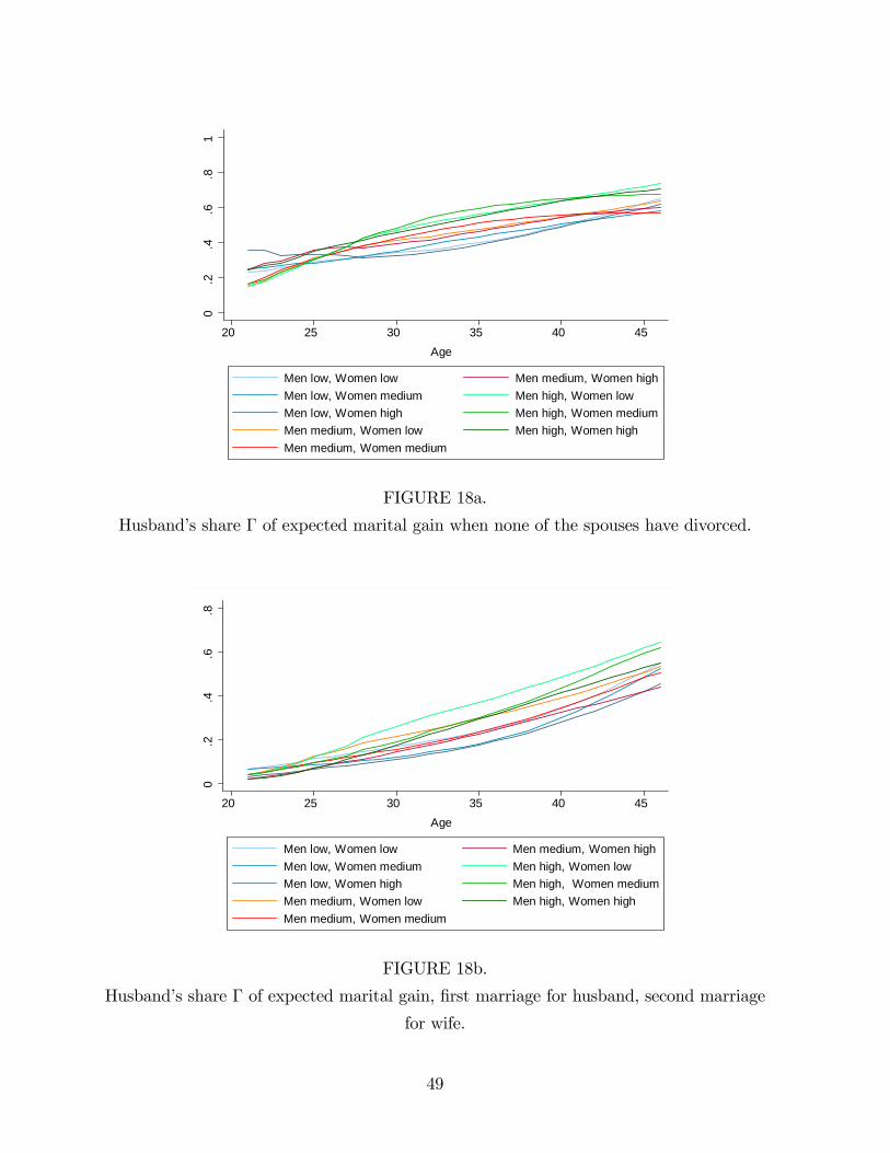
0.2

.4.6

.81

20 25 30 35 40 45Age


FIGURE 18a.

Husband�s share � of expected marital gain when none of the spouses have divorced.

0.2

.4.6

.8

20 25 30 35 40 45Age


FIGURE 18b.

Husband�s share � of expected marital gain, �rst marriage for husband, second marriage

for wife.

49

.5.6

.7.8

.91

20 25 30 35 40 45Age


FIGURE 18c.

Husband�s share � of expected marital gain, second marriage for husband, �rst marriage

for wife.

0.2

.4.6

.81

20 25 30 35 40 45Age


FIGURE 18d.

Husband�s share � of expected marital gain when both spouses have divorced.

50

the dynamics of marriage and divorce - iza institute of ...ftp.iza.org/dp6379.pdfthe dynamics of...

Documents