N A S A C O N T R A C T O R

R E P O R T

N A S A C R - 2 4 0 1

THE DYADIC DIFFRACTIONCOEFFICIENT FOR A CURVED EDGE

by R. G. Kouyoumjian and P. H. Pathak

Prepared by

THE OHIO STATE UNIVERSITY

ELECTROSCIENCE LABORATORY

Columbus, Ohio 43212

for Langley Research Center"?e-iai*

NATIONAL AERONAUTICS AND SPACE ADMINISTRATION • WASHINGTON, D. C. • JUNE 1974

https://ntrs.nasa.gov/search.jsp?R=19740020597 2020-03-23T06:06:13+00:00Z

1. Report No. 2. Government Accession No.NASA CR-2U01

4. Title and SubtitleTHE DYADIC DIFFRACTION COEFFICIENT FOR A CURVED EDGE

7. Auxnor(s)

R. 0. Kouyoumj ian and P. H. Pathak

9. Performing Organization. Name and AddressThe Ohio State University '.; ;

ElectroScience Laboratory

Columbus, Ohio '̂ 3212 ' • • ' ~ : : ' *

12. Sponsoring Agency .Name and Address , t l , . . •

National Aeronautics and Space AdministrationWashington, D. C. -.205U6

3. Recipient's Catalog No.

5. Report DateJune 1974

6. Performing Organization Code

8. Performing Organization Report No.AR 3001-3

10. Work Unit No.

502-33-13-02

11. Contract or Grant No.NGR 36-008-l!̂

13. Type of Report and Period Covered

Contractor Report

14. Sponsoring Agency Code

15. Supplementary Notes. ••* -

Progress report.

16.- Abstract .

'»A'compact dyadic diffraction coefficient for electromagnetic waves obliquely incident on acurved edge formed by perfectly-conducting curved or plane surfaces is obtained. This diffractioncoefficent;remains valid.in the transition regions adjacent to shadow and reflection boundaries,where the .diffraction coefficients of Keller's original theory fail. Our method is based onKeller's method of the canonical problem/ which in this case is the perfectly-conducting wedgeilluminated by plane, cylindrical, conical and spherical waves. When the proper ray-fixedcoordinate system is introduced, the dyadic diffraction coefficient for the wedge is found tobe'the sum of only .two" dyads,; and it is shown that this is also true for. the dyadic, diffractioncoefficient's of higher order edges. One dyad contains the acoustic soft diffraction coefficient;the othef dyad contains the acoustic hard diffraction coefficient. The expressions for the

- acoustic wedge, diffraction- coefficients contain Fresnel integrals, which ensure that -the totalfield is continuous at shadow and reflection boundaries. The diffraction coefficients have thesame form for the different types of edge illumination; only the arguments of the Fresnel

• integrals are different. Since diffraction is a local phenomenon, and locally the curved edgestructure is wed'ge shaped, this result is readily extended to the curved-edge; It is interestingthat even though the polarizations and the wavefront curvatures of the incident, reflected anddiffracted waves are markedly'different, the'total-field calculated from this high-frequencysolution for the curved edge is continuous at shadow and reflection boundaries.

" ' '

17. Key Words (Suggested by Author (s))

.;, Antenna's", Spacecraft and Aircraft^Antennas'/?•, -ili'- • ' : • > . i ' • > : • ; • * . • : . « . : • . . : . . • ; - .

Applied Electromagnetic Theory

19. Security dassif. (of this report

Unclassified

18. Distribution Statement

. Unclassified -Unlimited

. . - STAR Category 0 9

20. Security Oassif. (of this page) 21. No. of Pages 22. Price*

Unclassified . 92 $!*.00

For sale by the National Technical Information Service, Springfield, Virginia 22151

Page Intentionally Left Blank

CONTENTS

Page

I. INTRODUCTION 1

II. THE GEOMETRICAL OPTICS FIELD 6

III. THE EDGE DIFFRACTED FIELD 15

IV. DISCUSSION 54

APPENDIX

I THE CAUSTIC DISTANCE FOR REFLECTION 58

II THE EDGE CAUSTIC DISTANCE 68

III THE PLANES OF INCIDENCE AND REFLECTION 73

IV RECIPROCITY 76

REFERENCES 86

iii

I. INTRODUCTION

This report is concerned with the construction of a high-

frequency solution for the diffraction of an electromagnetic wave

obliquely incident on a curved edge in an otherwise smooth, curved,

perfectly-conducting surface surrounded by an isotropic, homogeneous

medium. The surface normal is discontinuous at the curved edge, and

the two surfaces forming the edge may be convex, concave or plane.

The solution is developed within the context of Keller's geometrical1 2 3theory of diffraction '* (referred to simply as the GTD henceforth)

so the dyadic diffraction coefficient is of interest. Particular

emphasis is placed on finding a compact, accurate form of the diffraction

coefficient valid in the transition regions adjacent to shadow and

reflection boundaries and useful in practical applications.

According to the GTD, a high-frequency electromagnetic wave incident

on a curved surface with a curved edge gives rise to a reflected wave,

an edge diffracted wave, and an edge excited wave which propagates

along a surface ray. Such surface ray fields may also be excited at

shadow boundaries of the curved surface. The problem is easily

visualized with the aid of Fig. 1, which shows a plane perpendicular

to the edge at the point of diffraction Q£. The pertinent rays and

boundaries are projected onto this plane. To simplify the discussion

of the reflected field we have assumed that the local interior wedge

angle is <_ IT. According to Keller's generalized Fermat's principle,

the ray incident on the edge Q? produces edge diffracted rays ed and

surface diffracted rays sr. In the case of convex surfaces the

surface ray sheds a surface diffracted ray sd from each point Q on its path.

ed

Fig. 1.

PLANE J. e AT QE

EDGE(SURFACE NORMAL

DISCONTINUOUS)

Incident, reflected and diffracted rays and their, -associated shadow and reflection boundaries projectedonto the plane normal to, the edge at the point ofdiffraction Q .

ES is the boundary between the edge diffracted rays and the surface

diffracted rays; it is tangent to the surface at Q£. SB is the shadow

boundary of the incident field and RB is the shadow boundary of the' • " ' . ' ':fs** ' '•.' ' ; ; .

reflected field, referred to simply as the reflection boundary hence-

forth. If both surfaces are illuminated, then there is no shadow

boundary at the edge; instead there are two reflection boundaries for

the problem considered here. Since the behavior of the ray optics

field is different in the two regions separated by a boundary, there

is a transition region adjacent to each boundary within which there

is a rapid variation of the field between the two regions.

'vv In the present analysis it is assumed that the sources and

field point are sufficiently removed from the surface and the

boundary ES so that the contributions from the surface ray field can

be neglected. The total electric field may then be represented as

in which "E1 is the electric field of the source in the absence of

the surface, "£*" is the electric field reflected from the surface with

the edge ignored, and E*^ is the edge diffracted electric field. The

functions u1 and ur are unit step functions which are equal to one in

the regions illuminated by the incident and reflected fields and to

zero in their shadow regions. The extent of these regions is determined

by geometrical optics. The step functions are shown explicitly in Eq. (1)

to emphasize the discontinuity in the incident and reflected fields at

the shadow and reflection boundaries, respectively. They are not included

in subsequent equations for reasons of notational economy.

The diffracted field as defined by Eq. (1) penetrates the shadow

region, which according to geometrical optics has a zero field, to

account for the non vanishing fields known to exist there. But the

correct high-frequency field must be continuous at the shadow and

reflection boundaries; hence the diffracted field must compensate

the discontinuities in the incident and reflected fields there.i*

In other words, the diffracted field must provide the correct

transition between the illuminated regions and the regions shadowed

by the edge.

The high-:frequency solution described ,in~th,e. next sections ,is..• " ' " • ' - - • ; • - - • " . . . • ''-• "- :*>£ • '

obtained in the following way. A Luneberg-Kline expansion for the

incident field is assumed to be given. The reflected field is- - ' - ? '.- '.

expanded similarly and related to the incident field by imposing

the boundary condition at the perfectly-conducting surface. Only.the

leading term, the geometrical optics term, is retained^.. Next the

general form of the leading term in the high-frequency solution for

the edge-diffracted electromagnetic field is determined. The wedge

(straight edge) geometry is treated first; its dyadic diffraction' ' • ' -' ; " - i .

coefficient is deduced from the asymptotic solution of,several canonical

problems. Some parameters in this diffraction coefficient are seen

to depend on the type of edge illumination. They are determined for

an arbitrary incident wave front by requiring the leading term in...

the total field to be continuous at the, shadow and reflection boundary.

It is found that only a slight extension of the solution for,the wedge

is needed to treat the more general problem posed by the curved edge.

This report is the third in a series of reports dealing with

edge diffraction. In the first report . the Pauli-Clemmow method of

steepest descent was employed in a manner different from that

employed by Pauli to obtain a more accurate asymptotic solution for

the field diffracted by a wedge. We showed that our, generalized Pauli

expansion can be transformed term by term into a generalized form of

the asymptotic expansion given by Oberhettinger . The .leading term

in our expansion was found to be more accurate than the leading term

in Oberhettinger's expansion; furthermore, our leading term for the

diffracted field contains a simple correction factor, which permits

the f ield to be calculated easily in the transition region. This

property is of considerable practical importance, because it enables

one to use the geometrical theory of diffraction in the transition

regions without introducing a supplementary solution. The correction

factors, referred to here as transition functions are simply included

with the diffraction coefficient.

In the first report only the scalar problem of plane waves

normally incident on the edge of wedge is considered. In the second.•*?•• .Q

report this work is extended to obtain a dyadic diffraction coefficient

for a perfectly-conducting wedge illuminated by obliquely-incident

plane, cortical, and spherical waves. By introducing the natural,

ray-fixed coordinates, the dyadic diffraction coefficient obtained

from each of these canonical problems is reduced to the sum of two

dyads. In other words, the matrix formed by the elements of the

dyadic diffraction coefficient is a two by two diagonal matrix.

The diagonal elements of this matrix are simply the scalar dif-

fraction coefficients, D^ and D, for the Neumann (hard) and

Dirichlet (soft) boundary conditions, respectively. The transition

functions appearing in D and D. have the same form for the four

types of illumination; in each case only a Fresnel integral is

involved. However the argument of the Fresnel integral depends

upon the type of illumination. Outside of the transition regions these

factors are approximately one, and Keller 's expressions for the dif-

fraction coefficients are obtained. The asymptotic solutions

described in this paragraph help us formulate the solution for a

more general type of i l luminat ion of the wedge, as noted earlier.

The analysis of wedge diffraction has had a lengthy history. -

Only a few of the reports and papers have been mentioned thus far.

Many of the more important papers on this subject may be found in

references 9, 10. A good review of wedge diffraction and the special

case of half plane diffraction is given in Chapters 6 and 8 of

referenced. Recently Anluwalia, Boers ma, and Lewis have written some

papers '* of special relevance to the work described here. References

11 and 12 describe high frequency asymptotic expansions for scalar waves

diffracted by curved edges in plane and curved screens and • '"•"'•'

reference 13 extends this work to a curved edge in a curved surface.

The authors make use of ray coordinates, and some of their results

dealing with rays and wavefronts have been helpful in the development

of our solution. Nevertheless, there are some noteworthy differences

between their solutions and this one, apart from the fact that their

problem is scalar instead of the vector problem treated here. Their

formulation or ansatz begins with the total field, and the

resulting correction of the ordinary GTD solution in the transition

region is different from ours. It appears that our result is the

more convenient to apply.

II. THE GEOMETRICAL OPTICS FIELD

The geometrical optics field, which is the sum of the leading

terms in the asymptotic expansions for the incident and reflected

fields, is a part of our high frequency solution for the edge

diffraction. The asymptotic expansions for the incident and

reflected fields are presented in this chapter; the results are

not new and;so they may-be familiar to the reader, but they are

included here for the sake of completeness and continuity in the

discussion. . . . . . . ,

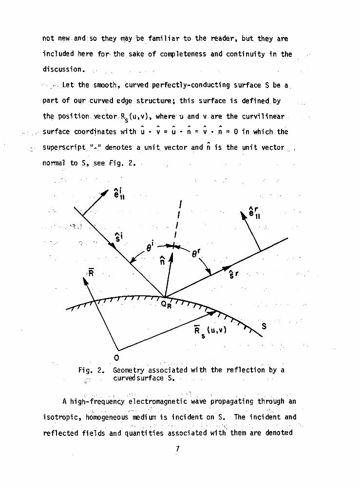
- Let the smooth, curved perfectly-conducting surface S be a

part of our curved edge structure; this surface is defined, by

the position vector R_(u,v), where u and v are the curvilinear^ A ^ A ^ A

surface coordinates with u • v = u • n = v • n = 0 in which the

superscript 'V denotes a unit vector and n is the unit vector

normal to S, see Fig. 2.

Fig. 2. Geometry associated with the reflection by acurved surface S.

A high-frequency electromagnetic wave propagating through an

isotropic, homogeneous medium is incident on S. The incident and

reflected fields and quantities associated with'them are denoted

7

by the superscripts (or subscripts) i and r, respectively. The

boundary condition on the electric field at S is

(2) fixU1(^)H-Er(T?s)]= 0 .

Since we are interested in an asymptotic high frequency solution,

the incident and reflected fields are expanded in Luneberg-Kline

series for large u>

(3)(jo))

where an eja) time dependence is assumed and k = co/v with v the

phase velocity of the medium. The electric field is a solution

of

(4)

subject to the condition that

(5) v • F = 0.

Substituting Eq. (3) into Eqs. (4) and (5) and equating the

coefficient of each power of u> to zero, one obtains the eikonal

equation

(6) |7*f- 1,

together with the transport equations

<7 a>

(7b) Is Em + F (v2*)Em = 2^^-" m = Y>2»3

whose solutions must also satisfy- ' r " " j j • v . ' ; x _ -

(8a) 4^^.-=.0.,

(8b) s • Em = vpv • E_ m = 1,2,3 •••.,.

where v^ =,s a unit vector in the direction of the ray path, which

is normal to the wavefront ^(R") = constant, and s is the distance

along the ray path.

We are interested here in the solution at the high frequency

l imit , where the asymptotic approximation for T reduces to

(9) F(s) * e - J s E0(s)

Equation (7a) is readily integrated, and after some manipulation

one obtains14'15

in which s=0 is taken as a reference point on the ray path and p,,

P2 are the principal radii of curvature of the wavefront at s=0.

In Fig. 3 PI and p2 are shown in relationship i ;to the rays .and.

the

Eq.cur, equatfon , ,

probation for the magnetic field is

ff

'_

Yc =s the characteristic admittance of the redi„, and

t is glven by Eq. (9).

Employing Eq. (6),

ds = ds;

consequently,

CAUSTICS

3. Astigmatic tube of rays.

10

FrorirEqs. (10), (12) and (9) one obtains the leading term in the

asymptotic expansion

(13) F(s) ̂ T (o ) c " ) , 2 e'J'ks( \ 6 ) t(s) * I ( O ) e e

which is -recognized; as the geometrical optics field; this could have

been deduced from classical geometrical optics employing power

conservation in the tube of rays shown in Fig. 3.

It is apparent that when s = -p, or -pp Eq. (13) becomes infinite

so that it is no longer a valid approximation. The congruence of

rays at the lines 1-2 and 3-4 of the astigmatic bundles of rays is

called a caustic. As we pass through a caustic in the direction of

propagation the sign of p+s changes sign and the correct phase shift

of +TT/2 is introduced naturally. Equation (13) is a valid high

frequency approximation on either side of the caustic; the field atx:> *.*

a caustic must be found from separate considerations ' .

Returning how to our problem of reflection at the ..perfectly-

conducting surface S, the incident field is known thus the E"m(R~0,

are known. The E^(Fs)-a/e f°unc' by using the boundary condition.

We take the; surface S as the reference point on the reflected ray

so s = 0 there; furthermore let- us modify our notation for. the

incident field at point of, reflection QR on S, denoting it by

^(QR). Now substituting Eq. (3) into Eq. (2) and equating like

powers of co,

11

(14) n x^(QR)e . -1 R + ,n xrlJJ(o)e- ,J- . = 0,

If this equation is to be satisfied for all m, then

(15) ^.(QR) = *r(o),

and since the above is true for every point on S,

/\ ^

(16a) u • Vi|>. (QD) = u • Vij; (o),

'• i

^ . ys

(16b) v • Vip.(Q-) = v • v\t

(17a) s1 • u = sr • u,

(17b) '.s1 • 0= sr - v .

Thus s1 and sr have the same projection on the plane tangent to S. -, • . • • ' . " : ' . - _ • " - ' - " . • " ' - , <4.

at QR, which leads us to the law of reflection:

The plane of incidence is defined by the incident ray and the

normal to the surface at the point of incidence. -The reflected ray

lies in the plane of incidence and the angle of reflection er equals

the angle of incidence e1, where both angles are measured from the

normal to the surface as shown in Fig. 2.

12

To determine ET(o) it is convenient to introduce the unit vectorA • ' ' '• *Vl

e± perpendicular to the plane of incidence and the unit vectors e,,

and e£, which are parallel to the plane of incidence and perpendicular

to s1 and sr, respectively, so that

08) e. x s = e.

in each case. Then we may set

at the surface. Employing Eqs. (15) and (19) in Eq. (14) we obtain

(20)

where "R~ is the dyadic reflection coefficient. In matrix notation

the reflection coefficient has a form familiar for the reflection

of a plane electromagnetic wave from a plane, perfectly-conducting

surface

(21) R =1 0

0 -1

This is not surprising if one considers the local nature of high-

frequency reflection, i.e., the phenomena for the most part depends

on the geometry of the problem in the immediate neighborhood of Q.

13

Thus the surface S can be approximated by its tangent plane at QR,

and the wavefront of the incident field by a plane wavefront.

It follows from Eqs. (13), (15) arid (20) that the geometrical

optics reflected electric field

(22)

in which ''pT and p£ are the principal radii of curvature of the

reflected wavefront at the point of reflection QR. In Appendix I

these radii of curvature are found to be a function of the incident

wavefront curvature, the aspect of incidence and the curvature of

S at QR. In this appendix it is shown that the expressions for

pT and pT can be put into the form

(23*1 L.jfV

i

• • •

where p} and p^ are the principal radii of curvature of the incident

wavefront at QR and

P1

with X, and X« unit vectors in the principal directions of the

14

incident wavefront, U, and.^ unit, vectors in the principal directions

of S at QD, and R-,,R~ the principal radii of curvature of S at QD.K • i£: . ' : • . • ' • : • - ' , .'.•• • K. .' "(

Equations (23a,b) are reminiscent of the simple mirror formulas of

elementary physics; this is particularly true in the case of an

incident spherical wave, where PI = P? = s' and ^ i» f? are foca^

distances independent of the range of the source of the spherical

wave.

In principle the geometrical optics approximations can be

improved by finding the higher order terms ETT(R), r£(R}, ••• in

the reflected field, but in general it is not easy to obtain these

from Eqs. (7b), (8b), (14) and. (15). Furthermore, these terms do

not correct the serious errors in the geometrical optics field

resulting from the discontinuities at reflection and shadow boundaries.

In the next section we will construct high-frequency approximations

for the edge diffracted field which in combination with the geometrical

optics field yield a continuous total field. :

III. THE EDGE DIFFRACTED FIELD

The smooth surface S has a curved edge formed by a discontinuity

in its unit normal vector. Points on the edge are defined by the

position vector r. When an electromagnetic wave is incident on .

the edge a diffracted wave emanates from the edge. The leading,

term in the .high frequency approximation for the electric field is

assumed to have the form - r; ' ;

(24) E

15

Substituting the above expression for E into Eqs. (4) and (5), and

again equating the coefficient of each power of o> to zero, one obtains

(25) |V| - 1, '

(26) d_

(27) s-A = 0,

and from the discussion in the preceding section, it follows that

(28)

in which

(29)7T

and s is the distance along the diffracted ray from a reference point

O1 which is not a caustic of the diffracted ray, see Fig. 4.

It is convenient to locate the reference point of the diffracted

ray at the edge point Qr from which it emanates; however the edge is. . . • " • £ . • • • -. . .

a caustic of the diffracted field. On the other1 hand, it is clear

that It (s) given by Eq. (28) must be independent of the location

of O1, hence

lim E^O1) V? exists.P'+O , ;

Furthermore E^(s) is proportional to the incident electric field at

Qc, so we may setc i

16

(30) limp'-»C

11 = E (QE) • D »

where D is the dyadic edge diffraction coefficient, which is analogous

to the dyadic reflection coefficient of the preceding section.

DIFFRACTEDRAY

(31)

EDGE

Fig. 4.

Thus the edge diffracted electric field

>~~ Q-Jks1" . I J

in which p is the distance between the caustic at the edge and the

second caustic of the diffracted ray.

In appendix II it is shown that

" i"t "\1 1 1 1 f U " ( s - s )1 - ' '-l e x '

17

wherein p^ is the radius of curvature of the incident wavefront at

Qc taken in the plane containing the incident ray and e is the unit

vector tangent to the edge at QE, n is the associated unit normal

vector to the edge directed away from the center of curvature, a>0

is the radius of curvature of the edge at QE, and 3k is the angle •-,•

between the incident ray and the tangent to the edge as shown in

Fig. 5a. Equation (32) is seen to have the form of :the elementary

mirror and lens formulas in which f is the focal distance. If p is—

positive, there is no caustic along the diffracted ray ^path; however

the caustic distance p is negative if the (second) caustic lies

between QE and the observation point. The diffracted field calculated

from Eq. (31) is not valid at a caustic, but as one moves outward from

Qc along the diffracted ray, a phase shift of +ir/2 is introduced

naturally after the caustic is passed as in the case of.the geometrical

optics field. .

:Since the high frequency diffracted field has a caustic at the

edge Eq. (31) is not valid there, and we can not impose a condition at

Qc to.determine "D in a manner similar to that used >tb find R". Never-

theless, the matching of the phase functions at the edge

(33) 4,.(QE) = *r(QE> = 4/d(QE)

is a necessary condition, which yields some useful information about

the solution. Since the phase is matched at each point on the edge,

it follows from Eq. (33) that

: e • v . ( Q ) = e • V i ; ( Q ) : = ; e > . v , )

18

i.e".,

A AI A *Y* * *•(34) -r> e • s = e • s = e • s .

The angle of incidence in this case is e defined earlier and shown

in Fig. 5a, cos BQ = e • s1, 0 <_ 3Q <_T\/2. The angle of diffraction

g. Is the angle-between the diffracted ray and the tangent to the

edge at QE; cos ed = e' • S, 0 <_ 3d'<. ir/2. Keller's law of edge dif-

fraction follows from Eq.(34).

The law of edge diffraction; the angle of diffraction B. is equal

to the;angle of incidence 3 , so that the diffracted rays emanating

fromiQc form a.cone whose half angle is 3 and whose axis is the

tangent:to the edge. The incident ray and the ray reflected from

the-surface at QE also lie on the cone of the diffracted rays.

The form of the dyadic diffraction coefficient will be treated

next. If ,an edge-fixed coordinate system is used to describe the

components of the incident and diffracted fields, it has been found

that-the dyadic diffraction coefficient is the sum of seven dyads[18,19];

in matrix form this means that the diffraction coefficient is a 3 x 3

matrix with 7 non-vanishing elements. However from Eqs. (8a) and (27)

it is apparent that if a ray-fixed coordinate system were used in place

of the edge-fixed coordinate system, the diffraction coefficient would

reduce to a 2 x 2 matrix, so that no more than four dyads would be

required. A further reduction in the number of dyads can be anticipated

if the proper ray-fixed coordinate is chosen. Recall that this kind of

simplification is achieved in the case of the dyadic reflection coefficient,

19

EDGE- FIXEDPLANE OF

INCIDENCE

h'v

PLANE OFDIFFRACTION

(0)EDGE

PLANE JL e AT QE

nir (b )

Fig. 5.

20

if the incident and reflected fields are resolved into components

parallel and perpendicular to the planes of incidence and reflection,

respectively, where the plane of reflection, which contains the normal

to the surface and the reflected ray, coincides with the plane of

incidence. Analogous planes of incidence and diffraction can be defined

in the; present case;

The plane of incidence for edge diffraction, referred to simply

as the edge-fixed plane of incidence henceforth, contains the incident

ray and the unit vector e tangent to the edge at the point of incidence

Qr. The plane of diffraction contains the diffracted ray and e.

These planes are depcited in Fig. 5; they are azimuthal planes with

respect to the polar axis containing e, and their positions can be

specified by the angles V and <j> shown in Fig. 5b. The unit vectors

(fi1 and $ are perpendicular to the edge fixed plane of incidence and

the plane of diffraction, respectively. The unit vector s1 E s1 is

in the direction of incidence at the edge and the unit vector s is in

the direction of diffraction. The unit vectors e^ and JL are parallel

to the edge fixed plane of incidence and the plane of diffraction,

respectively, and

(35a,b) g' = s1 x < f> ' , s = s x < j> . .

Thus the coordinates of the diffracted ray (s,ir-e0,<{>) are

spherical coordinates and so are the coordinates of the incident ray

(S ' ,B 0 »< f> ' )» except that the incident (radial) unit vector points toward

the origin Q.

21

, According to Keller's theory[3] the diffraction coefficient for

a curved edge may be deduced from a two-dimensional canonical problem,

involving a straight edge, where the cylindrical surfaces which form

the edge are defined by the boundary curves depicted in Fig. 5b, 'In*;-

the present discussion the edge may be an ordinary edge formed by a

discontinuity in the unit normal vector, an edge formed by a discontinuity

in surface curvature, or an edge formed by a discontinuity in some:higher

order derivative of the surface. :

Consider the z-components of the electric and magnetic fields; in:

the presence of this surface with an edge

(36a)

(36b)

Ez =

V Hz + Hz»

they satisfy

(37) (V*

H.

"= 0

together with the soft (Dirichlet) or hard (Neumann) boundary

conditions

8H(38,39) Ez = 0 or ^ = 0,

respectively, on the boundary curve and the radiation condition

at infinity. The a/an is the derivative along the normal to the

boundary curve.

22

Starting with the high frequency solutions for the z-components

of the diffracted field

(40) K: A(R),

and-;substitutirig these into Eq. (37), and employing the methods

described earli.er, the: asymptotic solutions may be put into the form

(41)<„<

El °s"̂

Hz Dh

r - l pVS(P+S)

in which D is referred to as the soft scalar diffraction coefficient

obtained when the soft boundary condition is used, and D^ is referred

to as the hard scalar diffraction coefficient obtained when the

hard boundary condition is used.

Since

(42a) E1. = E1, sin s ,

(42b) Y c E , s in

(43a) sin

(43b) sin

with 1/Y = Z = / vi/e the characteristic impedance of the medium,

23

it follows from Eqs. (41), (42), and (43) that

-d

(44)

E'o

Ed S(P+S) e-Jks .

'*consequently, the dyadic diffraction coefficient for an ordinary (or

higher order) edge is a perfectly-conducting surface can be expressed

simply as the sum of two dyads

/ . _ » = *• * „ * I A I %(45) D = -B B D - $ $ DL

to first order. Since Ds and Dh are the ordinary scalar diffraction

coefficients which occur in the diffraction of acoustic waves which en-

counter soft or hard boundaries, we see the close connection between

electromagnetics and acoustics at high frequencies. Also, it follows that

the high frequency diffraction by more general edge structures, and by thin

curved wires can be described in the form given by Eqs. (44) and (45).

The balance of this report is concerned with finding expressions

for D and D^ which can be used in the transition regions adjacent to

shadow and reflection boundaries in the case of diffraction by an

ordinary edge. Recently Keller and Kaminetzky[20] and Senior[21]

have obtained expressions for the scalar diffraction coefficients in

the case of diffraction by an edge formed by.a discontinuity in

surface curvature and Senior[22] has given the dyadic (or matrix)

diffraction coefficient in an edge-fixed coordinate system. Keller

and Kam1netzkey[20] also have given expressions for the scalar

diffraction coefficients in the case of higher order edges.

The diffraction by a wedge will be considered first; the straight

edge serves as a good introduction to the more difficult subject of

diffraction by a curved edge. As noted earlier, the dyadic diffraction

24

coefficient can be found from the asymptotic solution of several

canonical problems, which involve the illumination of the edge by

different wavefronts. It is not difficult to generalize the resulting

expressions for the scalar diffraction coefficients to the case of

illumination by an arbitrary wavefront.

A. The Wedge

When a plane, cylindrical, or conical electromagnetic wave is

incident on a'perfectly-conducting wedge, the solution may be

formulated in terms of the components of the electric and magnetic

field parallel to the edge; we will take these to be the z-components.

••''' In the case of a spherical wave it is convenient to use the z-components

of the electric and magnetic vector potentials. These z-components

may be represented by eigenfunction series obtained by the method of

Green's functions. The Bessel and Hankel functions in the eigenfunction

series are replaced by their integral representations and the series

are then summed'leaving the integral representations. Integral

representations for the other field components in the edge-fixed

coordinate system are then found from the z (or edge)-components ,

except in the case of the incident spherical wave, where the integral

representations of the field components are obtained from the z-components

of the vector potentials. These integrals are approximated asymptotically

by the Pauli-Clemmow method of steepest descent[23], and the leading

terms are retained. The field components are then transformed to the

- ?ray-fixed coordinate system described previously. The resulting expression

for the diffracted field can be written in the form of Eq. (31) which

'makes it possible to deduce the 'dyadic diffraction coefficient TJ.

25

The asymptotic solutions outlined in this paragraph are presented in

detail in reference [8],

Summarizing the results given in. Reference [8]

(46) E^s) *r1(QF) • T(s.s') A(s)e' jks

in which A(s) describes how the amplitude of the field varies along

the diffracted ray; • •

— for plane, cylindrical and conical waveincidence (in the case of cylindrical wave

(47) A(s) =1

/incidence, s is replaced by r = s sin BQ

the perpendicular distance to the edge),

/s (s '+s) for spherical wave incidence.

It follows from Eq. (32) that P = Pe for the wedge. In the case of

plane, cylindrical and conical waves p* is infinite and in the case:eTof spherical waves p = s'. The dyadic diffraction coefficient

"0(5,5') has the form given in Eq. (45), which supports the assumptions

leading to that equation.

If the field point is not close to a shadow or reflection

boundary, the scalar diffraction coefficients

(49 f" ' -je

TT

4 sin £ni2Trk sin BQ

1cos ^ - cos

7 1•/•(b-d)1 \ IT / d)H

( n J c o s n - - c o s ( r^)_

for all four types of illumination, which is important because the

diffraction coefficient should be independent of the edge illumination

away from shadow and reflection boundaries where the plane surfaces

forming the wedge are <f>=0 and 41 = n-ir. The wedge angle is (2-n)ir; see

26

Fig. 5b. This expression becomes singular as shadow or reflection

boundaries are approached, which further aggravates the difficulties

at these boundaries resulting from the discontinuities in the incident

or reflected fields. The above scalar diffraction coefficients have

been given by Keller[3].

Grazing incidence, where <t> ' = 0 or nir must be considered separately.

In this case D = 0, and the expression for D. given by Eq. (4) must be

mult ipl ied by a factor of 1/2. The need for the factor of 1/2 may be

seen by considering grazing incidence to be the l imit of oblique

incidence. At grazing incidence the incident and reflected fields merge,

so that one half the total field propagating along the face of the wedge

toward the edge is the incident field and the other half is the reflected

field. Nevertheless in this case it is clearly more convenient to regard

the total field as the "incident" field. The factor of 1/2 is also

apparent if the analysis is carried out with <)>' = 0 or nir.

Combining Eqs. (31), (45) and (49) it is seen that the diffracted-1/2f ield is of order k ' with respect to the incident and reflected fields.

At high frequencies this means that the diffracted field is in general

weaker than the incident and reflected fields, at aspects not close to

shadow and reflection boundaries.

To simplify the discussion, the wedge angle has been restricted so

that 1 < n <_2\ however, the solution for the diffracted field may be

applied to an interior wedge where 0 < n < 1. The diffraction coef-

ficient vanishes when

sin v- = 0; —

27

hence for n = 1, the entire plane, : -

n = 1/2, the interior right angle,

n = 1/M, M = 3,4,5 •• • , interior acute angles,

the boundary value problem can be solved exactly in terms of the in-

cident field and a finite number of reflected fields, which may ,be

determined from image theory. Moreover as n -» 0, even with the

presence of a non-vanishing diffracted field, the phenomenon is

increasingly dominated by the incident and reflected fields.

Returning now to the subject of exterior edge diffraction, :the

total field changes rapidly in the vicinity of shadow and reflection

boundaries. In the case of the shadow boundary its behavior is

predominantly that of the incident field on the illuminated side,

whereas it is that of the diffracted field, emanating from1 the-edge,

on the shadow side. For example if the wedge is illuminated by a plane

wave perpendicular to its edge, the total field varies from an

essentially plane wave behavior to a cylindrical wave behavior in

the vicinity of the shadow boundary. These regions of rapid field

change adjacent to the shadow and reflection boundaries are

referred to as transition regions. In the transition, regions the~~~ — — • - J . .'".I

magnitude of the diffracted field is comparable with the incident

or reflected field, and since these fields are discontinuous at-, - Vi . -

their-boundaries, the diffracted fields must be discontinuous at

shadow and reflection boundaries for the total field to be continuous

there.

28

An expression for the dyadic diffraction coefficient of a

perfectly-conducting wedge which is valid both within and outside

the 'transition regions[8] is provided by Eq. (45) with

-J f(50) D (ft.+'-.B ) e

°

c o t - F [ k L a + ' l f r c o t - F[kL

F[kL a+

I . V "" )where

00

(51) F(X) = 2jJYejX I e-JT dt

in which one takes the principal (positive) branch of the square root,

and

(52) aVf.) = 2 cos22

in which N1 are the integers which most nearly

satisfy the equations

(53a) 21rnN+-((j)±<j)1) = ir

and

(53b) 2TrnN"-(<{)±4>1) = -IT .

The above expression for the soft (s) and hard (h) diffraction

coefficients contains a transition function F(X) defined by Eq. (51),

29

where it is seen that F(X) involves a Fresnel integral. The

magnitude and phase of F(X) are shown in Fig. 6, where X = kLa.

(54a)

(54b) 0 < phase F(X) < Tr/4

When

(55) X > 10,

F(X) 21 1 . '

If the arguments of the four transition functions in Eq. (51) exceed

10, so the transition functions can be replaced by unity, Eq. (50) ;r

reduces to Eq. (49).

(56) X = kL a±(<(.±<{,1)

in which L is a distance parameter, which was determined for several

types of illumination. It was found that

(57) L =

2s sin B for plane wave incidence,

r r'—+ i for cylindrical wave incidence,

cc ' 2r sin B for conical and spherical waves + s1 -111 Mo

incidence,where the cylindrical wave of radius r1 is normally incident on the

edge, and r is the perpendicular distance of the field point from

the edge. A more general expression for L, valid for an arbitrary

wavefront incident on the straight edge, will be determined later.

30

(S33H93C1 ) 3SVHd

o

o

CO

I

O)•r—

31

The largeness parameter in the asynptotic approximation used to

find Dg is kL. For incident plane waves the approximation has

been found to be accurate if kL > 1.0, unless n is close to one,

then kL should be > 3.

a~(<j> ± < t> ' ) is a measure of the angular separation between the

field point and a shadow or reflection boundary. The + and - super-

scripts are associated with the integers N+ and N~, respectively,

which are defined by Eqs. (53a,b). For exterior edge diffraction

N = 0 or 1 and N" = -1, 0 or 1. The values of N~ as functions of

n and B = 4 ± <f>' are depicted in Figs. 7a and 7b; thes.e integers are

particularly important near the shadow and reflection boundaries

shown as dotted lines in the figures. It is seen that N~ do not

change abruptly with aspect $ near these boundaries, which is a

desirable property'.' The trapezoidal regions bounded by the solid

straight lines represents the permissible values of 3 for 0 <_ $,

<j>' <_ nu with 1 <_ n <_ 2.

At a shadow or reflection boundary one of the cotangent functions

in the expression for Dg giver, by Eq. (50) becomes singular; the other

three remain bounded. Even though the cotangent becomes singular, its

product with the transition function will be shown to be bounded.

However let us first note the location of the boundary at which each

cotangent becomes singular; this information is presented compactly

in Table 1. The locations of the shadow and reflection boundaries when

only one surface of the wedge is illuminated and when both surfaces of

the wedge are illuminated are shown in Figs. 8a, b, c below Table 1.

32

N---I

1.5

N"*0

*""" H* 2ir 3ir 4ir

(b)

Fig. 7. N" as functions of e and n.

33

TABLE 1

The cotangent is singularwhen

value of Nat the boundary

cot (**(*-*2n •-1) <j>= <j) - TT , a SB .

surface 4>=0 is shadowed N+ = 0

cot 2n<|>= (f)1 + ir, a SBsurface cpmr is shadowed N" = 0

cot 'liUjVA <|> = (2n-l)ir-(j)1, a RBreflection from surface <b=m\ N+ = 1

<t>=Tr - (j)1 , a RBreflection from surface $=Q N" = 0

77770

rnr

Fig. 8. Shadow and reflection boundaries for differentangles of incidence < f> ' .

34

Since discontinuity in the geometrical optics field at a shadow or

reflection boundary is compensated separately by one of the four terms

in the diffraction coefficient, there is no problem in calculating the

field when two boundaries are close to each other or in juxtaposition.

This occurs when $' = 0 or mr and when <t>' is close to nir/2 with n ;v i.

The shadow and reflection boundaries are real if they occur in physical

space, which is in the angular range from 0 to mr; outside this range

they are virtual boundaries. If a virtual boundary is close to the

surface of the wedge, as it is when <f>' is close to TT or (n-l)ir, its

transition region may extend into physical space near the wedge and

significantly effect the calculation of the field there. The value

of N or N" at each boundary is included in Table 1 for convenience;

as noted earlier, this is a stable quantity in the transition regions.

Next it will be shown that the product of the cotangents.and the

transition functions in Eq. (50) is finite, even at the shadow and

reflection boundaries. To facilitate the discussion let

(58) e = <(. ± <t>' . : • • ' . • : ; •

In the neighborhood of the shadow or reflection boundary

(59) 3 = 2ir nN* + (TT - e),

where e is positive in the region illuminated by the incident or

reflected field. The ± superscript of N is directly associated with

the + sign in the equation above and the ± sign in the argument of

the cotangent below.

35

For e small,

(60) cQt(*rir-4, fa,

and2

e*\, -g

- 2

The transition function F(X) is given by Eq. (51) with X = kLa±(B).:

We are concerned with the case where kL is large but X is small, so that

(62) F(X) 7- 2XeJ * - X

From Eqs. (60), (61) and (62),

2 "J * '* + X)

(63) cot*2J=- F[kL a

i -2TrkL sgn e - 2kLee

for e small. It is clear that the above expression is finite but

discontinuous at the shadow and reflection boundaries. These

discontinuities compensate the discontinuity in the incident or

reflected field at these boundaries, as will be shown in the

paragraphs to follow.

The high frequency approximation for the total field being con-

sidered here is the sum of the geometrical optics field and the

asymptotic approximation of the diffracted field. It is convenient

to give the components of these fields in the ray fixed coordinate

system described on page 21; hence it will be necessary to transform

36

the components of the reflected field given in the first section to

this coordinate system. We will begin by carrying out this trans-

formation, which is facilitated by employing matrix notation.

From Eqs. (21) and (22) the reflected electric field

(64)"Er"

£i o"

0 -1

"EnlII

E] f(s).

rfhere the subscripts u and j. denote components parallel and per

pendicular to the ordinary plane of incidence and

(65) f(s) = ,-Jks

p£Note that for the plane surfaces forming the wedge, p =

where p^, p^ are the principal radii of curvature of the incident

wavefront at the point of reflection. Equation (64) may be written

more compactly as

(66) Er * RE1 f(s) .

The ordinary plane of incidence and the edge- fixed plane of incidence

intersect along the incident ray passing through Q£. The ordinary

plane of incidence, the edge-fixed plane of reflection, and the cone

of diffracted rays intersect at the ray reflected from Q£. The edge-

fixed plane of reflection contains the tangent to the edge and the ray

reflected from QE. These planes and their lines of intersection are

depicted in Fig. 9.

37

EDGEFIXEDPLANE OF

REFLECTION

INCIDENTPLANE

EDGE FIXEDPLANE OFINCIDENCE

REFLECTEDRAY

INCIDENT RAY

Fig. 9. Edge fixed plane of incidence and reflection.

Let the angle between the edge-fixed plane of incidence and the

ordinary plane of incidence be -a. In Appendix III it is shown that

the angle between the edge-fixed plane of reflection and the ordinary

plane of incidence is a. The components of the incident electric field

parallel and perpendicular to the edge-fixed plane of incidence are

(67a) E1. = E1 cos a - E] sin aD-. " J-

(67b) E\ '= E,1, sin a + E] cos a

or in the more compact matrix notation

38

(68) E1' = T(-o)E1

where

(69) T(-a) =COSa -SlHa

Sina COSa

From Eq. (66) the reflected electric field

(70) Er * R E1 f(s) H(e).

in the neighborhood of the reflection boundary

(71) H(e) = Sgn e)

is the unit step function.

The components of the reflected field parallel and perpendicular to

the edge-fixed plane of reflection are given by

(72) T(a)Er = [T(a)RT(-a)-1][T(-a)E1] f(s) H(e)

From Eq. (69) and R as given in Eq. (21)»

(73) T(a)R T(-a)"1 = R;

hence from Eqs. (68), (70), (72) and (73)

39

(74) f(s) (1 + sgn e).

The diffracted field close to the reflection boundary at <t> = -n-b*

is given by Eq. (31) together with Eqs. (50) and (63)

(75) 1 fl Ol

? 1° -ij JTsin 60

"Isfp1 + s)

e"jks sgn e +

+ terms which are continuous at this boundary.

For the total field to be continuous at the reflection boundary,

the sum of the discontinuous terms in Eqs. (74) and (75) must vanish;

hence

(76) - sin Bs(Pi + s)

e-jks + f(s) = Qj

so that the distance parameter

s(p1e + s) p] PJ sin2BQ

+ s)(77)

The behavior of the incident and diffracted fields at the shadow

boundary $ = it + <j>' may be treated in the same manner. . After passing

beyond QE» the electric field of the incident ray in the neighborhood

of the shadow boundary is

(78) 1 [-1 ol7 [0 -ij f(s) (1 + sgn e)

The diffracted field close to this shadow boundary is

40

(79) -'*- "*

JT I Pe -jfcs51

s(p

e sgn e +e '

+ in terms which are continuous at this shadow boundary.

For the total field to be continuous at the shadow boundary, the sum

of the discontinuous terms in Eqs. (78) and (79) must vanish, and again

it is seen that L is given by Eq. (77). Equation (77) is also obtained

when the leading term in the high frequency approximation for the total

field is made to be continuous at the other shadow and reflection

boundaries. Also Eq. (77) reduces to Eq. (57) for the several types

of incident waves for which formal asymptotic solutions were derived.

We conclude therefore that the expression for L given by Eq. (77) is

correct when the wedge is illuminated by an incident field with an

arbitrary wavefront whose principal radii of curvature are p^j and p^.

Since kL is the large parameter in the asymptotic approximation,

3 can not be arbitrarily small, which precludes grazing and near grazing

incidence along the edge.

The commentary on Eq. (49) in the case of grazing incidence along the

surface of the wedge also applies to Eq. (50), i.e., the diffraction

coefficient D. is multiplied by a factor of 1/2 and the diffraction

coefficient D = 0.

If n = 1 or 2, it is apparent from Eq. (52) and the integral values

of N* that

(80) a1^) = a(e) = 2 cos2

Thus

41

(81) cot \ F[kLa+(g)]

F [kLa(0)]

-2 sin

cos - - cos £F [kLa(B)] ,

and from Eq. (50) the expressions for the scalar diffraction coefficients

reduce to

(82)

"J 4 . ire sin-

n>/2~irk sin $FDcLaU-*1)]

- if , (*-<('1co. n co. n

_ nklau+,,n' rn- "" • rn- ^+(')l '

The edge vanishes for n = 1 and the boundary surface is simply a perfectly-

conducting plane of infinite extent. It is seen that the diffraction

coefficients and diffracted field vanish for this case as expected.

If n = 2 the wedge becomes a half plane and \

(83) Ds(*,*';80) =

-J-e

2J2Trk sin 0, cos cos

which can be written in the form

42

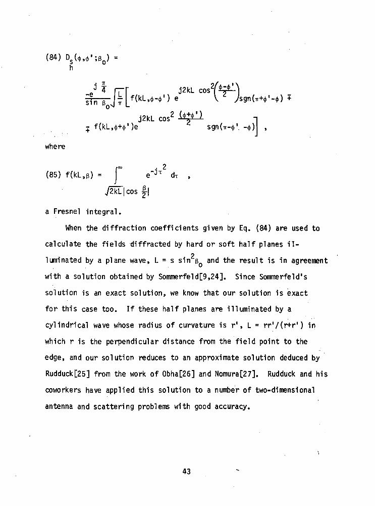
(84) Ds

h

sin

2j2kL cos

sgnU-ffi1 -((>) ,

where

. 2(85) f(kL,B) = I e"jT dT ,

cos72<L|

a Fresnel integral.

When the diffraction coefficients given by Eq. (84) are used to

calculate the fields diffracted by hard or soft half planes il-2

luminated by a plane wave, L = s sin R and the result is in agreement

with a solution obtained by Sommerfeld[9,24]. Since Sommerfeld's

solution is an exact solution, we know that our solution is exact

for this case too. If these half planes are illuminated by a

cylindrical wave whose radius of curvature is r1, L = rr'/(r+r') in

which r is the perpendicular distance from the field point to the

edge, and our solution reduces to an approximate solution deduced by

Rudduck[25] from the work of Obha[26] and Nomura[27]. Rudduck and his

coworkers have applied this solution to a number of two-dimensional

antenna and scattering problems with good accuracy.

43

In this section on diffraction by wedges, diffraction coefficients

have been obtained which may be used at all aspects surrounding the

wedge, including the transition regions adjacent to shadow and

reflection boundaries. The diffraction by curved edges in plane

surfaces and curved sheets will be considered in the next section.

B. The Curved Edge

The diffraction by curved edges will be treated in this section.

As in the preceding section our solution is based on Keller's method•v

of the canonical problem. The justification of the method is that

high-frequency diffraction like high-frequency reflection is a local

phenomenon, and locally one can approximate the curved edge geometry

by a wedge, where the straight edge of the wedge is tangent to the

curved edge at the point of incidence QE in Figs. 5a,b, and its plane

surfaces are tangent to the surfaces forming the curved edge. The

reflection coefficient for the curved surface derived in Section I

could have been found by this method, choosing the reflection of plane

waves at a plane surface as the canonical problem. With these

assumptions, the results of the preceding section can be applied

directly to the curved edge problem. As we have just noted, there is

an equivalent wedge (with exterior wedge angle nir) associated with every

curved edge structure, and so in generalizing the solution for the wedge,

it is only necessary to modify the expressions for the distance parameter

L, which appear in the arguments of the transition functions.

In the present treatment we do not'show that our solution can be

matched to a boundary layer solution valid at and near the curved edge.

44

It .would be desirable to carry this out to confirm the validity of our

solution and possibly to obtain additional terms in the asymptotic

approximation. Ahluwalia has used a boundary layer solution in this

way to obtain an asymptotic expansion for the scalar field diffracted by

a curved edge;, however his representation of the total field differs

from the one given here. It does not appear as separate contributions

from the incident, reflected and diffracted fields.

The diffraction by a curved edge in a plane screen affords the

simplest example of curved edge diffraction. The scalar diffraction

coefficients appearing in Eq. (45) are given by Eqs. (83) or (84), and

since p = p1 on both the shadow and reflection boundaries, L is the

distance parameter given by Eq. (77). At aspects other than incidence

and reflection, p within the square root term of Eq. (31) must be

found from Eq. (32). As in the case of the wedge, we obtain a high-

frequency approximation at all points surrounding the edge, which

are not too close to the edge or to caustics of the diffracted

field.

The diffraction by a curved edge in a curved screen (n=2) is

next in the order of increasing difficulty. Whenever the surface

forming the edge is curved, the region near it is dominated by surface

diffraction phenomena, which is particularly important on the convex

side. On the convex side of the curved screen there are surface

ray modes, also known as creeping waves, which shed energy tan-

gentially as they propagate along the surface. As a result of this,

the radiation leakage phenomenon is significant in a considerable region

45

near the surface. On the concave side of the curved screen we have

bound modes that do not leak energy as they propagate; these modes"

are known as whispering gallery modes. Both types of modes are

excited by an illuminated edge in a curved surface; however they also

may be excited by the incident field. As mentioned earlier, surface

diffraction phenomena have been neglected in the present treatment;

hence the region between the convex surface and the boundary ES

between the edge diffracted and surface diffracted rays must be ex-

cluded. The boundary ES is formed by the intersection of the cone of

diffracted rays and the plane tangent to the surface at Q^; in general

it does not lie in the ordinary plane of incidence. In addition, the

transition region adjacent to the boundary must be excluded. This>

region from which the field and source points are to be exluded appears

as the shaded portion of Fig. lOa, where all rays and boundaries are

shown projected on the plane perpendicular to the edge at Qr. It should

be noted that in general the projection of the surface ray S does not

coincide with the intersection of the boundary surface S and the plane

of projection.

On the concave side the whispering gallery effect can be

described approximately by geometrical optics in the form of a series

of reflected waves whose rays form cords along the concave reflecting

surface as indicated in Fig. lOb. As glancing incidence is approached,

the cord length diminishes and the description of the phenomenon in

terms of a sequence of reflections breaks down; the geometrical optics

analysis must be truncated at this point. If the errors resulting

46

from this truncation are not serious, the radiation from the concave

side.can be included in the present analysis.

\\\\ srSB

(a) CONVEX SIDE

(b) CONCAVE SIDE

Fig. 10. Diffraction at the edge of a curved screen.

In this case n = 2, and the scalar diffraction coefficients in Eq,

(45) are given by

47

(86) D U,$';n

-J-e Fpcl^aU-f')] j F[kLraUV)3

in which the first term is discontinuous at the shadow boundary, whereas

the second is discontinuous at the reflection boundary. Unl ike the

reflection from a plane surface, the divergence or spreading of the wave

reflected from a curved surface is different from that of the incidence

wave; hence the radii of curvature of the reflected and diffracted wave-

fronts at the shadow boundary are distinct from the radii of curvature

of the incident and diffracted wavefronts at the shadow boundary.

Employing arguments similar to those used to f ind the distance parameter

for the wedge

(87a)s(pe+s) p]. sin £

where

r rSlnr

=

pi, pi are defined as before, pi" and p« are the principal

radii of curvature of the reflected wavefront at QE, and from Eq. (32)

(88) ^pe

2(n.ne)(s'*n)

a sin2R

48

As iji1 approaches TT we approach grazing incidence as shown in

Fig. 11. Then since pTp£ -»• 0, Lr -* 0 and Eq. (86) can no longer be

used to calculate the scalar diffraction coefficients. Under these

circumstances the shadow and reflection boundaries usually lie within

the shaded region in Fig. 11, and the transition regions associated

with edge diffraction overlap those associated with surface diffraction.

If the field and source points are both sufficiently far from the edge,

we may set the transition functions in Eq. (86) equal to unity. On- ?• '

the otherhand, for the field point or source point close to the edge

or for both points close to the edge, we may be able to use reciprocity

(see Appendix IV) to calculate the field at P in Fig. 11, if the distance

parameters for a unit source located at P are large enough.

/ —' SHADOW ANDSB REFLECTION BOUNDARY'S

FOR A SOURCE AT P

Fig. 11. Grazing incidence on the edge of a curved screen.

49

We conclude this chapter by finding the scalar diffraction coef-

ficients for a curved edge in an otherwise smooth curved surface. Again

we seek diffraction coefficients which can be used in the transition

regions associated with the shadow and reflection boundaries of this

structure. Both surfaces forming the curved edge may be convex, both

surfaces may be concave, one surface may be convex and the other concave,

or one surface may be plane and the other convex or concave.

First let us consider the simple case which occurs when the

illuminated surface forming the curved edge is plane, as it may be at

the base of a cylinder or cone. For this configuration the reflected

field is found directly from the incident field, as it is in the case

of the wedge, e.g., it may be easily deduced from image theory. Thus

the scalar diffraction coefficients are found directly from Eq. (50) and

the distance parameter from Eq. (77). The calculated diffracted field may

not be accurate close to the shadowed surface if surface diffraction

phenomena are significant.

The more general problem where the illuminated surface is curved

is closely related to the diffraction by a curved edge in a curved

screen which has just been discussed; for example, the field point

and source point must not be too close to a convex surface and the

case of grazing incidence must be treated separately.

We introduce the wedge tangent to the boundary surfaces of the

curved edge at Q£. The boundary ES is formed by the intersection of

this wedge with the cone of diffracted rays. Away from the boundary

ES on the cone of diffracted rays the scalar diffraction coefficients

are given by Eq. (50), except that distance parameter L in the argument of

50

each of the four transition functions may be different. As before L

is found in each case by requiring the total field to be continuous

at each shadow and reflection boundary.

It is seen from Figs. 7a,b that N , N" associated with the shadow

boundaries at (f»'-ir, <J>'+TT are different from zero only at angular

distances greater than TT from these boundaries. When this angular

distance exceeds TT the field point is usually outside the transition

region in question, unless kL is small. In view of the assumptions

involved in extending the wedge solution to the curved edge, the validity

of the approximation is in question for such small values of kL, so

they are excluded here. These considerations and analogous con-

siderations lead us to set the N* equal to the values they have in

Table I.

Then . TT

e 4(89) DU.o'-Bj =-ST= xS , O

h 2nj2irk sin

2 sin F

TT.cos — - cos n )F[kLrna+(<»V )> cotH ***')) F[kLroaUV

in which a(e) = 2 cos

and a+(e) = 2 cos2 .

Again employing arguments similar to those used to find the distance

parameters for the edge, one finds that L1 is given by Eq. (87a), and

that I/0, L™ are given by Eq. (87), The additional superscripts o

and n denote that the radii of curvature are calculated at the re-

flection boundaries TT-^' and (2n-l )TT-<|>', respectively.

51

Although the reasoning employed to find the distance parameters is

the same as that used in the preceding cases, namely that the total

field be continuous at the shadow and reflection boundaries, a problem

arises which was not encountered earlier. For a given aspect of in-

cidence it is clear that only two of the boundaries associated with thei' *•*

three transition functions exist, the other boundary is outside real

space. Since neither the field or source points are permitted close to

grazing incidence at $' = 0 or mr, it is reasonable to set the transition

function, which is associated with the boundary located outside the

interval 0 < <j> < nir, equal to one.

At grazing incidence $' = IT or (n-l)ir for which Lro or Lrn vanish,

the scalar diffraction coefficients are calculated by the same procedure

used for the curved screen at grazing incidence <j>* = ir.

In the far zone where s » the principal radii of curvature p,, p«

of the incident and reflected wavefronts at QE and the radius of curvature

p of the diffracted wavefront at Qr in the directions of incidence and

reflection, Eqs. (77), (87a), and (87b) simplify to the form

. 2p,p? sin R

(90) L--L2- 2. .'e

the appropriate superscripts are omitted here for the sake of-notational

simplicity.

An interesting case occurs if there is a caustic of the incident,

reflected or diffracted wave on a shadow or reflection boundary. The

radii of curvature p,, p2 or p associated with such a caustic are negative,

and L may be either negative or positive. If L is positive, the presence of

caustics at these boundaries presents no difficulty, except at points near

52

the caustic itself. On the otherhand if L is negative, there is a

problem because the transition function has two branches each with an

imaginary argument. We will restrict our attention to the situation where

all the caustics on the boundary lie between the field point and the edge;

this may occur in far-zone field calculations for example.

As pointed out in the last paragraph of Appendix II, if L is negative-, -

the incident (or reflected) field has one more caustic on the shadow (or

reflection) boundary than does the diffracted field. This means that the

phase of the transition function must change by an additional -n/2 as one

moves from a point outside the transition region to the boundary, so that

the transition function must have a total phase variation of 3ir/4 instead

of the ir/4 phase variation shown in Fig. 6. An examination of the two

branches of the transition function at the boundary and outside the

transition region reveals that they do not have the proper behavior.

When a curved strip is illuminated by a plane wave from its concave

side, there is a caustic of the reflected field on the reflection boundaries.

In treating the scattering from this strip we have found that an adequate

function is provided by

|F(k|L|a)|e j3Cphase of F(k L a)]

in which F(k |L |a) is the ordinary transition function given by Eq. (51).

(Note that L and a may have superscripts). In spite of the fact that

the above expression has the proper behavior outside transition regions

and at shadow or reflection boundaries and also appears to yield good

numerical results, it lacks theoretical justification. A satisfactory

derivation of the transition function for L negative is being sought.

53

IV. DISCUSSION

A dyadic diffraction coefficient has been obtained for an

electromagnetic wave obliquely incident on a curved edge formed by

perfectly-conducting curved or plane surfaces. Unlike the edge

diffraction coefficient of Keller's original theory, this diffraction

coefficient is valid in the transition regions of the shadow and

reflection boundaries. Although the diffraction coefficient has

been given in dyadic form in the earlier chapters, it can also be

represented in matrix form, so that the high-frequency diffracted

electric field can be written

(91)

r.d i'3, 0

0 -D,'h-J

"E1 "eo'

- A1 -

/ P

J,S(p+S.)

and since the high-frequency diffracted magnetic field

(92) = Yc s x

(93)

,d 1

LH

-D.

-Du -Hi -..I i P iJs(P+s)

in which D , D. are given by

(a) Eq. (89) for the curved edge (general case),

(b) Eq. (86) for a curved edge in a curved screen,

(c) Eq. (83) or (84) for a curved or straight edge in a plane screen,

and p is given by Eq. (32).

54

(d) Eq. (50) for the wedge,

It is pointed out in Section IIIB that the scalar diffraction

coefficients in cases (a) and (b) are not valid at aspects of

incidence and diffraction close to grazing on a convex surface

forming the edge at the point of diffraction. Work is in progress

to remove this limitation. Also grazing incidence on a plane

surface is a special case which requires the introduction of a

factor of 1/2 when calculating the diffracted field, see the

discussion of page 27.i rThe large parameters are kl_ or kL , kL in the asymptotic

approximation; hence when these are small our GTD representation

of the diffracted field is no longer valid. Thus source or field

points close to the edge (s or s1 small) must be excluded; also

aspects of incidence close to edge-on incidence (e small) must be

excluded. Edge-on incidence is a separate phenomenon, which has

been discussed by Ryan and Peters [28] and by Senior [29].

Outside of the transition regions where the arguments of the

transition functions are greater than 10, the expressions for the

scalar diffraction coefficients all simplify to Eq. (49). Usually

the field point is only in one transition region at a time, so

that the calculation of the diffracted field is simplified because

only one of the transition functions is significantly different from

unity.

One would expect the diffraction coefficients for the wedge to

be more accurate than those for the curved edge, because the

canonical problems involve wedge diffraction. If the curved edge

55

were used as a canonical problem, one would anticipate the presence

of additional terms in the asymptotic solution for the diffracted

field; these terms would depend upon the radius of curvature of

the edge at the point of diffraction and its derivatives with

respect to distance along the edge. This is verified by the work

of Buchal and Keller [30] and Wolfe [31], who treated the diffraction

of a scalar plane wave normally incident on a plane screen with ai

curved edge.

In calculating the diffracted field, it is assumed that the in-

cident field is slowly varying at the point of diffraction, except

for its phase variation along the incident ray. If the incident field

is rapidly varying at the point of diffraction, it is usually possible

to express it as a sum of slowly-varying component fields, so that

the diffracted field of each component can be calculated in the usual

way and the total diffracted field obtained by superposition. Al-

ternatively, in calculating the diffracted field, one could introduce

higher order terms which depend upon the spatial derivatives of the

incident field at the point of diffraction. Expressions of this type

were obtained by Zitron and Karp [32] in their treatment of the

scattering from cylinders; they are also derived in Reference 11.

In the text it is pointed out that Eqs. (91) and (93) can not be

used to calculate the field at a caustic of the diffracted ray. At

such a caustic it is convenient to use a supplementary solution in

the form of an integral representation of the field. The equivalent

sources in this representation are determined from a suitable high-

frequency approximation, such as geometrical optics or the GTD. In

56

the case of an axial caustic, it is convenient to employ equivalent

electric and magnetic edge currents introduced by Ryan and Peters [33];

the use of these edge currents is also described in Reference [34].

In conclusion we note that the geometrical optics field and

our expression for the edge-diffracted field are both asymptotic

solutions of Maxwell's equations. The total high-frequency field

is the sum of these two fields, and away from the edge it is

everywhere continuous, except at caustics. Our solution reduces

to known asymptotic solutions for the wedge, and it has been found

to yield the first two or three terms in the asymptotic expansion

of the diffracted fields of problems which can be solved differently.

Furthermore, the numerical results obtained by its application to

a number of examples are found to be in excellent agreement with

rigorously-calculated and measured values. Also we have been able

to show that our solution is consistent with the reciprocity

principle, see Appendix IV.

57

APPENDIX I

THE CAUSTIC DISTANCE FOR REFLECTION

The principal radii of curvature of the reflected wavefront

pC, pi and the principal directions (axes) of the wavefront will be

determined in this appendix. The plane of incidence may be different

from the principal planes of the reflecting surface, so that the

principal directions of the incident wavefront are quite distinct

from those of the reflecting surface.

This problem has been treated both by Fock [35] and by Deschamps; [36]

however they did not find the principal radii of curvature nor the

principal directions of the reflected wavefront. Fock used a surface-

fixed coordinate system to formulate his solution, and he evaluated

the resulting 3x3 determinant for the divergence factor D(S) of the

reflected wave after some rather complicated tensor analysis. On the

otherhand, Deschamps formulated his solution in a ray-fixed coordinate

system,* and employing elementary matrix theory together with straight-

forward coordinate transformations, he obtained a 2 x 2 curvature matrix

for the reflected wave from that of the incident wave. We will find

pT, p£ and their principal directions by diagonalizing his curvature

matri x.

Let us begin by defining the curvature matrix employed by

Deschamps. Consider the curved surface

*The advantages inherent in using ray-fixed coordinate systems intreating ray optical problems have already been noted in the text.

58

(A-1) z = f(x,y)

with the z axis normal to the surface at the point P where x,y,z = 0.

Thus

(A-2) fx = fy = 0

where

are evaluated at x,y = 0.

In the neighborhood of the origin

(A-3) z = i [f x2 + 2f xy + f y2]f- AA Ajr yy

-, U2 V2'

in which p,, pp are the principal radii of curvature in the principal^ *> . •

directions X, Y respectively. With

x = x x + y y a n d X " = X X + Y Y . .

Eq. (A-3) may be written in matrix notation

(A-4) z = £x Q x = ^-X QQ X,

in which Q is a 2 x 2 symmetric matrix and Q is its diagonal form.

The matrices Q and Q are referred to as curvature matrices

59

(A-5) Q =

"fXX

fL xy

and

" i

(A-6) Qft =w

i

P?

0L

fxy

fyyJ

-0

ii

^J

The Gaussian curvature of the surface

(A-7) K = determinant of Q = |Q| = |QQ| .

Let a wavefront be incident on a curved surface S at QR as

shown in Fig. 2A.A A

U-|, U2 are unit vectors in the principal directions of S at ,QR

with principal radii of curvature R,, Ik.

*i "iX-,, X2 are the principal directions of the incident wavefront:at

QR with principal radii of curvature pJ, pi.

x!f, xT are unit vectors perpendicular to the reflected ray; they

*i ~iare determined by reflecting the unit vectors X,, X2 in the plane tangent

to S at QR, i.e.,

(A-8) xlj" = X] - 2(n - X])n,2 2 2

see Fig. 2A. As will be seen, x x« are not in the principal directions

of the reflected wavefront. We now define

60

f ( x , y )

Fig. 1A. A smooth curved surface near the point P.

(A-9)pl

0P2

(A-10) Cr

and

0

(A-ll) 0 ="i

" 2 -

Deschamps has shown that the curvature matrix for the reflected wavefront

(A-12) Qr = Q0 - cos e

61

Fig. 2A. Geometry for the analysis of the reflectedwavefront. The reflecting surface is S.

Intersection of a principalplane of S at QR with SIntersection of the plane ofincidence with the planetangent to S at QR

_ Extension of the Reflected raybelow S.

62

in which the superscript -1 denotes the inverse matrix, the superscript

T denotes the transpose matrix and e1 is the angle of incidence as before.

A result equivalent to Eq. (12) has been obtained by Fock.

(A-13) Qr =

where

(A-14a) Q^ = -U-pl

2 cos e

eR-,

/A(A- >" 2 COS 912 = —-2

Q22912 ^ el!022Rl

(A-14c)P2

2 cos e1

l e 2

(e1?)2 (0n)

2if. , 1 1R

T h1 ^^

with

(A-Hd) 'a, i.X • Uk.

We have diagonalized Qr to find its eigenvalues l/pr,

63

(A-15) 1_= ifl 1 V cose1

r <T\ T "T I , .2PI \PI P2y lei L[< ° 2 2 > 2 <h <v2

Rl

4 cose

01R

lieR

in which the + sign associated with pT and the - sign with pi". As noted

in the discussion following Eqs. (23a,b) in the text, this equation has

the form of an elementary mirror formula, except that the reciprocal of

the object distance is replaced by the mean curvature of the incident/

wavefront.

The incident spherical wavefront is frequently of interest; let

us simplify Eq. (A-15) for this case. For the spherical wave x|, X^Aican be chosen in any way convenient. Let X, be in the plane of

Aiincidence; X« is then parallel to the plane tangent to the surface of

reflection at QR. Referring to Fig. 2A,

A*i i A i * "i A

(A-16a) X-, = -cos e sin u> U, + cos e cos o» U« + sin e n,

(A-16b) Ci cos U U1 + sin

where u is the angle between the plane of incidence and the n, u« principal

plane of the reflecting surface.

64

(A-77a) Q _°17 - - cos

the above Eqs.

(A-78) |ni .7 ; le| - - cos

furthermore

(M9b)

tence, substituting Eqs.and v n - i M i •»«*. rtq.

65

(A-20) -!- =

with

Tr

pl

1 + ]

s cos e1

sin e2

[ Rl ._

sin2e1

u

*2 J

1

cosV

r p 2 "1sin e. sin e

D D

1 ^

2.,4R1R2

(A-21a) sin e = cos ui +- scos e ,

,_2(A-21b) sin e = sin u + cos a> cos e .

01 is the angle between the direction of the incident ray s1 and U,,A ^ A

whereas e? is the angle between S and,Up. Equation (A-20) was obtainedt - - •" .' £, • • _

by Kouyoumjian several years earlier using a different method.

We conclude this section by giving the eigenvectors,..of Q ;

these yield the principal directions of the reflected wavefront with

respect to the Xp x£ coordinates.

[(Q22 - ^ ) x,r - ((A-22) Xr =

pl

pl^12

(A-23) = -sr x

66

xi

Fig. 3A. Principal directions of the reflected wavefront withrespect to the xr, x£ coordinates.

It should be noted that the principal directions of the wavefront

are distinct from the principal directions associated with the reflection

matrix; as pointed out in the text the latter are parallel and perpendicular

to the plane of incidence.

67

APPENDIX II

THE EDGE CAUSTIC DISTANCE

Fig. 4A. Caustic distances associated with the diffractionby a curved edge.

A wavefront is incident on a curved edge at the point Q£, where

the radius of curvature is a, the unit tangent vector is e, and the

unit normal vector to the edge is n given by the Serret-Frenet formula

(A-24) e = -

in which the super dot denotes differentiation with respect to the distance

along the edge and a is taken to be positive. It is apparent from the

above equation that n is directed away from the center of curvature.

68

A second useful formula will be derived next. Let r be the position

vector from a point 0 to a point on the edge.

(A-25) e = "r

(A-26) r = 7/r

from which

(A-27) r = £- \ r .r

Since

(A-28) r2 = 7 • 7 ,

(A-29) r = 7 • r ,

where Eq. (A-26) has been used.

.Substituting Eqs. (A-25), (A-26) and (A-29) into Eq. (A-27) and

dot multiplying both sides of the resulting equation by e, one obtains

(A-30) e • r=] "

According to Keller's law of edge diffraction,

A A A A

(A-31). s1 • e = s • e = cos 6

and so

69

(A-32) s1 • e + e • s1 = s • e + s • e :

"i

Employing Eqs. (A-24) and (A-30) in Eq. (A-32) .

(fl.33) i - ( • •»•• ) . J i i i - . - . i -»• • «v.Jg-ii-- : -1 ot p d ,

pe '

where p^ = s1 is the radius of curvature of the incident wavefront at

QE taken in the plane containing the incident ray and e,

p is the caustic distance; it is also the radius of curvature

of the diffracted wavefront at Qr taken in the plane containing

the diffracted ray and e.

Using Eq. (A-31), Eq. (A-33) may be written more compactly as

11 n • (s 1 - s )(A-34) 1 = -U- - -£—-£

pe o ',

which has the same form as the elementary lens equation, where p' and p

correspond to the source and image distances, respectively. Thus we

may write Eq. (A-34) as

(A-35) 1-W

where f is interpreted as the focal distance. Eq. (A-34) was first given

by Kouyoumjian [8], and it has also appeared in a number of ElectroScience

Laboratory reports [34,37], Recently Deschamps has rederived Eq. (A-34)

by a different method [36],

70

An alternative expression for p has been given by Keller [3];

we will derive it here for the sake of completeness.

From Eq. (A- 31 )

Again using Eqs. (A-25), (A-30) and (A-31 )

2 * "sin R r\ • d

(A'36) . - - J — = - s i n -

(A-37)

Here 6 is the angle between n and the diffracted ray.

It has been found more convenient to calculate the edge caustic

distance p from Eq. (A-34), which does not contain any derivatives.

Since the edge is a caustic of the diffracted rays, it is clear

that one of the principal directions of the diffracted wavefront lies

in the plane of diffraction and is perpendicular to the diffracted ray.

The other principal direction is perpendicular to the plane of diffraction

and is thus tangent to the cone of diffracted rays. At a distance s from

the point QE on the edge the principal radii of curvature of the dif-

fracted wavefront are p + s and s.

In general, the principal directions of the incident and reflected

wavefrpnts associated with rays incident and reflected at Qr (recall that

these rays lie on the cone of diffracted rays) do not coincide with the

principal directions of the diffracted wavefronts associated with rays.

71

diffracted in the directions of incidence and reflection. However in

the edge-fixed planes of incidence (or reflection) the curvature of the

diffracted and incident (or reflected) wavefronts is the same. The

relationship of the diffracted wavefront to the incident wavefront at

the shadow boundary is apparent from Eq. (A-34); on the shadow boundary

s = s1 and so p = p^. The relationship between the diffracted wavefront

and the reflected wavefront on the reflection boundary could be deduced

from Eqs. (A-15) and (A-34), but it may be verified more easily in the

following way. From Eq. (33) the reflected and diffracted phase

functions are the same along the edge, i.e.,

/(QE) - AQE) ;

hence

/(QE) + s = <|;d(QE) + s

in the plane containing the tangent to the edge e and the reflected,

diffracted rays at the reflection boundary. It follows that p = p£,

the radius of curvature of the reflected wavefront in the plane

containing the reflected ray and e. The relationships between the radii

of curvature of the diffracted wavefront and the incident and reflected

wavefronts at the shadow and reflection boundaries described in this

paragraph have been noted by Lewis and Boersma [12].

72

r •;£•-. . .APPENDIX I I I - . - • - . .

T, . ; THE PLANES OF INCIDENCE AND REFLECTION

j'.fT ; - . .- ;-s . . • ' •' . . - . - ; ,- • ' ' •_

In this appendix it will be shown that the angle a between the. . s ? r • • : ; " : , • • . - • - . . . ' . - . , - ; - • • •

edge-fixed plane of reflection and the ordinary plane of incidence is. '". f > V • ! v ' - / • " ' • " ' ' . - N - • •

equal to minus the angle between the edge-fixed plane of incidence and

the ordinary plane of incidence. We will refer to the ordinary plane

of incidence simply as the plane of incidence.• • ' . - . - . • . • • ' ' . . - : ' ' ! . ' I . . ' . - ' . * ' " ' * '

The plane of incidence contains the unit vectors s1 and n orA * . • • ! . ' • • : " . . ••• . • • • • . . ' / •s and n. The edge-fixed plane of incidence contains the unit vectors^ * . • • - ' • " . " 0 .^,?..' '

s1 and e. The edge-fixed plane of reflection contains the unit vectors«.p f.s and e. The plane of incidence and the edge-fixed plane of incidence

intersect along the incident ray at Q£. The plane of incidence and

the edge-fixed plane of reflection intersect along the reflected ray

at QE.A* A

Referring to Figs. 2, 5 and 5A and recalling that s = s1 at the

edge,

(A-38a)

(A-38b)

» I I / A A I \ i|s x (n x s ) I ,

•j" •A A A

o« = -s' x (e x s1)

|s' x (e x s ' ) | ,

(A-38C) e,; •" | s r x ( n x s r ) |

73

REFLECTEDRAY

PLANE OFINCIDENCE

EDGE-FIXEDPLANE OF

REFLECTION

EDGE- FIXEDPLANE OF

INCIDENCE

Fig. 5A. Geometry of the planes of incidence; edge-fixed incidenceand edge-fixed reflection. The incident and reflectedrays are perpendicular to the page and directed outward..-

(A-38d) ,| s r x ( e x s r ) |

Let a be the angle between the plane of incidence and the edge-

fixed plane of reflection, see Figs. 9 and 5A,

cosA A M A AM

_ -r * -(n • s )(e • s )a = e • R = — » — A A - „ ' Ar z[ l - ( n - s ) ] [ l - ( e . s ) ]

1Let a be the angle between the plane of incidence and the

edge-fixed plane of incidence,

74

(A-39) cos a1 = e1'

Since (n-s1) = -(n-sr) from the law of reflection and (e*s r) = (e*sr)

from the law of edge diffraction, it follows from Eqs. (A-38) and (A-39)

that

(A-40) - cos a1 = cos a;

hence

(A-41) a1 =±a .

From the definition of angles in Fig. 5A, a1 = -a.

75

APPENDIX IV

RECIPROCITY

The Lorentz reciprocity theorem imposes an important condition.on

the solution of an electromagnetic problem. This is a necessary con-

dition and approximate solutions which fail to satisfy it may contain' ' '" .' ' " - ' - . '; ' •;•••" "•" ,%

errors which are unacceptably large. We will develop the reciprocity

condition for the edge structure under consideration in this report,

and-see if the high-frequency solutions given in Chapter III satisfy'it.

Also it will be shown how reciprocity - may be used to ;extend our analysis

to a special configuration where it would not be valid if applied •

directly.

Let the sources g and g' radiate in the presence of an edge

structure as shown in Fig. 6A; the sources are positioned at a finite

distance from the edge and from each other. The surface S rests on the

perfectly-conducting boundary, except in the immediate vicinity of edge,

and extends to infinity. The surface Sm is the surface'at ̂ infinity; it

joins with S and together with this surface encloses the region occupied

by the sources g and g1. The surface S is sharply rounded at the edge

so as to enclose it tightly, but its radius of curvature does not vanish

there. *

The sources g and g1 consist of electric and magnetic current

moments which may be distributed in a volume, over a surface or along a

line, so that the infinitesimal electric current moment

76

(A-42a)

0 dv, in a volume

7 ds, over a surface

la d&, along a line

and the infinitesimal magnetic current moment

(A-42b) dp"m =m

KV dv, in a volume

T< ds, over a surface

M£ d£, along a line

:in which Jy is the volume density of electric current, 1( is the volume

density of magnetic current, etc. Starting with Maxwell's curl equations

in the form

(A-43a) v x F- jcoe F =

m(A-43b) -v xF+ jo>y H = -T-2Idv ,

with a little manipulation [38] in which the divergence theorem, is employed,

one obtains, .

?•* - . - JPsource g

|(F . dp; - F • dp;)source g1

(A-44) (ff x T1 - JT1 x I) • n ds ,

J7

where the source g1 and its fields are denoted by primes and the source

g and its fields are the unprimed quantities.

•

«

\

\

\ ./ SURFACE S./ ' SURFACE S

. X00

Fig. 6A. Region pertaining to the discussion on thereciprocity principle.

The fields of g and g1 satisfy an edge condition, also n x E,

n x P = 0 on the boundary surface; hence there is no contribution to

the surface integral in Eq. (A-44) from the integration over S. The

fields of g and g1 also satisfy a radiation condition, so the

integration over S in Eq. (A-44) vanishes too. Thus

78

(A-45)_ (P - dpe - ff- - dpm) = (F • dp; - F • dp;)source g source g1

* . i i - "•

which is a statement of reciprocity in integral form. Since the above

must be true for any distribution of the sources g, g1,

(A-46) E' ydpe - H1 • dpm = E • dp; - H • dp;

It is well known that the geometrical optics field satisfies the

reciprocity condition. Since the total field is the sum of the geometrical

optics field plus the diffracted field it follows that the diffracted

field also satisfies the reciprocity condition; in other words

(A-47) t> • dpe - tf- - dpm = t • dp; - tf • dp; .

Now let us see if the GTD solution for the diffracted field satisfies

Eq. (A-47). We .wil l first consider the reciprocity relationship for a

pair of incremental electric current moments dp" , dp"1. The electric

field of dp"; incident on the edge is

it JKZ _~JKS „ * i(A-48) T1 (QE) = -^- S-jr- s1 x (s1 x dp"e)

(A-49) F1 • dp"e = a"1 - D(<M';30) • a h(s .s ' )

(A-50) E* • dp' = a - D (4, ' , ,»;«) • a1 h(s ' ,s)

79

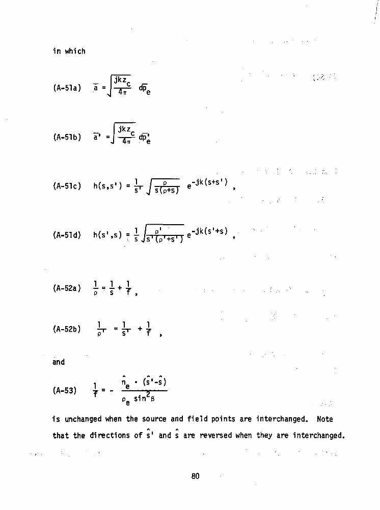
in which

(A-51a) a = Hrr

(A-51b) a' =

(A-51c) h(s.s')- lr f̂ =; e-J"<s+sl>

(A-5!d)

(A-52a) =

(A-52b)

and

(A-53)sin

is unchanged when the source and field points are interchanged. NoteA A

that the directions of s1 and s are reversed when they are interchanged.

80

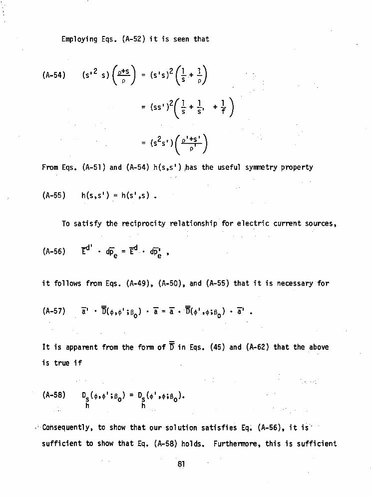
Employing Eqs. (A-52) it is seen that

(A.54)

From Eqs. (A-51 ) and (A-54) h(s,s ') ,has the useful symmetry property

(A-55) h(s,s') = h(s',s) .

To satisfy the reciprocity relationship for electric current sources,

(A-56) E • dpe =

it follows from Eqs. (A-49), (A-50), and (A-55) that it is necessary for

(A-57) a' • D(<M'iB0) • a = a ••"&($'.,4;eQ) • a1 .

It is apparent from the form of TJ in Eqs. (45) and (A-62) that the above

is true if

(A-58) Ds(<^,<frl;g0) = DsU',(f;B ).

h h

Consequently, to show that our solution satisfies Eq. (A-56), it is

sufficient to show that Eq. (A-58) holds. Furthermore, this is sufficient

81

to show that the general expression for reciprocity given by Eq. (Ar47)

is also satisfied, because if Eq. (A-58) is true it can be shown in a

manner analogous to the preceding development that H . • .dp" = H •-,• dp~̂

Vfe will examine the scalar diffraction coefficients for wedge ,

diffraction first. Referring to Eq. (50), the quantity

F[kL

remains unchanged if $ and <f>' are interchanged. The quantity

also remains unchanged, because the two terms are interchanged if <|> and

<j>' are interchanged. This can be shown by noting that when $ and $' are

interchanged

N+ is replaced by - N~,

N" is replaced by - N ,

thus a+U'~<|>) = a"U-^1)

and a"(*l-((i) = a (<j>-<j>')

For the sources dpg, dp^

(A-59) L = ^-^r sin2eQ,

82

so that it is invariant with respect to an interchange of points defined

by ? and ?'.

From the preceding discussion it is clear that the scalar

diffraction coefficients for the wedge satisfy Eq. (A-58); hence

our GTD solution for the diffraction of an electromagnetic wave by

a perfectly-conducting wedge is consistent with reciprocity both

within and outside the transition regions.

Turning next to the scalar diffraction coefficients for the

curved edge in the curved screen, it is apparent that Eq. (86) is

unchanged when $ and <j>' are interchanged. We note that L1 is in-

variant with respect to an interchange of source and observation

points, because it is given by Eq. (A-59). Thus if the pair of sources

are positioned so that they are not in transition regions of each

others reflection boundaries, F[kLra($+$')] can be replaced by unity,

and Eq. (A-58) is satisfied. On the other hand, if the pair of

sources dp", dp"' are positioned on each other reflection boundaries,

the quantities

(A.60a) A.!h.itir.1^*1.p-|S PI 1

ir. s r s

(A-eoc) c = ps s p

83

are invariant when s and s1 are interchanged. Since

sin230,

it too must be invariant with respect to this interchange, with the result

that Eq. (A-58) is satisfied. Thus we have been able t6 show that our

GTD solution for the diffraction of an electromagnetic wave by a curved

screen satisfies the reciprocity condition everywhere except in the

transition region of a reflection boundary, and within this region it

satifies the reciprocity condition directly on the boundary itself. It

is therefore reasonable to assume that this solution is consistent with

reciprocity at all points where it is valid, with the possible ex-r

ception of some small departures from reciprocity at certain points ;

in the transition region of the reflection boundary.*

It is pointed out in the text that as <j>' approaches TT and one is

close to grazing incidence on the curved screen (see Fig. 11), the

solution for the diffraction coefficients given by Eq. (86) becomes

invalid, because Lr approaches o. However, we may use reciprocity to

calculate E ^ p ) in the following way. Set dp" equal to o and replace

dp" in Eq. (A-47) by a unit electric current moment u directed parallel

to the component of t (p) which is to be calculated; then for the

incremental sources dp' and dp"' at 0 in Fig. 11

*The solution may satisfy reciprocity at these points, but we havenot been able to show it.

84

(A-62) u 'z ITU- «•» HP FBI*- t-elxs-l.dp-Ls'. c ° e I ° J mj

in which D(<j>' ,<|>;BO) = -^Q DS(*' ,<(.;30)-JJlDh(<}.1 ,*;Bff)

and h(s',s) is given by Eq. (A-51d). It is assumed here that kl_r for

.Incidence from P is sufficiently large so that our approximation for

the diffracted field at 0 is valid. In Eq. (A-62) one would ordinarily

..let,

u =<

The discussion of reciprocity for the curved edge in the

otherwise smooth, curved surface follows in the same manner as

that for the curved edge in the curved screen. One concludes from

this that Eq. (89) satisfies Eq. (A-58) for all points at which the

scalar diffraction coefficients are valid, except possibly for some

points in the transition regions of the shadow boundaries, were small

deviations from reciprocity may occur. Also if a problem arises in

calculating the diffracted field near grazing incidence on a curved

surface (f1^)* this calculation may be carried out with the aid of

Eq. (A-62).

85

REFERENCES

1. J. B. Keller, "The Geometric Optics Theory of Diffraction,"•

presented-at the McGill Symposium on Microwave Optics, 1953,

Air Force Cambridge Research Center Report TR-59-118 (II)v

pp. 207-210. 1959.

2. J. B. Keller, "A Geometrical Theory of Diffraction," in Calculus

of Variations and its Applications, edited by L. M. Graves,

McGraw-Hill Book Co. (1958), pp. 27-52.

3. J. B. Keller, "Geometrical Theory of Diffraction," J. Opt. Soc.

Am., 52, pp. 116-130, 1962.

4. M. Kline, "An Asymptotic Solution of Maxwell's Equations,"1

Comm. Pure and Appl. Math., 4, pp. 225-262, 1951.

5. D. L. Hutchins, and R. G. Kouyoumjian, "Asymptotic Series

Describing the Diffraction of a Plane Wave by a Wedge/

Report 2183-3, 15 December 1969, The Ohio State University

ElectroScience Laboratory, Department of Electrical Engineering;

prepared under Contract AF 19(628)-5929 for Air Force Cambridge

Research Laboratories. (AFCRL-69-0412) (AD 699 228)

6. W. Pauli, "On Asymptotic Series for Functions in the Theory of

Diffraction of Light," phys. Rev., 54, pp. 924-931, 1938.

7. F. Oberhettinger, "On asymptotic Series for Functions Occurring

in the Theory of Diffraction of Waves by Wedges," J. Math.

Phys., 34, pp. 245-255, 1956.

8. P, H. Pathak and R. G. Kouyoumjian, "The Dyadic Diffraction

Coefficient for a Perfectly-Conducting Wedge," Report 2183-4,

5 June 1970, The Ohio State University ElectroScience Laboratory,

86

Department of Electrical Engineering; prepared under Contract

AF 19(628)-5929 for Air Force Cambridge Research Laboratories.

(AFCRL-69-0546) (AD 707 827) , , , •

9. J. J. Bowman, T. B. A. Senior and P. L. E. Uslenghi,

,. Electromagnetic and Acoustic Scattering by Simple Shapes,

North-Holland Pubishing Co., (1969).

10. D. S. Jones, The Theory of Electromagnetism, The Macmillan

, Co. (1964).

11. D. S. Ahluwalia, R. M. Lewis, and J. Boersma, "Uniform

Asymptotic Theory of Diffraction by a Plane Screen," SIAM

J. Appl. Math., 16, pp. 783-807, 1968.

12. R. M. Lewis and J. Boersma, "Uniform Asymptotic Theory of

Edge Diffraction," J. Math. Phys., 10, pp. 2291-2305.

13. D. S. Ahluwalia, "Uniform Asymptotic Theory of Diffraction

by the Edge, of a Three-Dimensional Body," SIAM J. Appl. Math.,

18, pp. 287-301, 1970. ; :

14. J. B. Keller, R. M. Lewis and B. D. Seckler, "Asymptotic

Solution of Some Diffraction Problems," Comm. Pure and Appl.

Math., 9, pp. 207-265, 1956.

15. R. G. ,Kouyoumjian, "Asymptotic High Frequency Methods,",

Proc. IEEE, 53, pp. 864-876, 1965. , ;

16. I. Kay and J. B. Keller, "Asymptotic Evaluation of the Field

at a Caustic," J. Appl. Physics, 25, pp. 876-883, 1954.; ,

17. D. Ludwig, "Uniform Asymptotic Expansions at a Caustic,"

.Comm. Pure Appl. Math, 19,.pp. 215-250, 1966.

87

18. J. B. Keller, "Diffraction by an Aperture," J. Appl. Physics,

;vol.:28, pp. 426-444, April 1957.

19. T. B. A. Senior and P. L. E. Uslenghi, "High-Frequency ;

Backscattering from a Finite Cone," Radio Sc., 6,

pp. 393-406, 1971. ;

20. L. Kaminetsky and J. B. Keller, "Diffraction Coefficients

for Higher Order Edges and Vertices," SIAM J. Appl. Math.,

22, pp. 109-134, 1972. ;

21. T. B. A. Senior, "Diffraction Coefficients for a.Discontinuity

in Curvature," Electronic letters, Vol. 7, No. 10, pp. 249-250,

May 20, 1971.

22. T. B. A. Senior, "The Diffraction Matrix for a Discontinuity in

Curvature," IEEE Trans., AP-20, pp. 326-333, 1972.

23. P. C. Clemmow, "Some Extensions to the Method of Integration by

Steepest Descents," Quart. J. Mech. and Appl. Math., 3, pp. 241-

256, 1950. : - -: ...

24. A. Sommerfeld, "Mathematische Theorie der Diffraktion," Math.

Ann., 47, pp. 317-374, 1896. ;

25. R. C. Rudduck, "Application of Wedge Diffraction to Antenna Theory,"

Report 1691-13, 30 June 1965, The Ohio State University

ElectroScience Laboratory, Department of Electrical Engineering;

prepared under Grant Number NsG-448 for National Aeronautics

and Space Administration. (Available as NASA CR-272, 1965.)

38

26. Y. Obha, "On the Radiation Patterns of a Corner Reflector,"

,-IRE Trans., AP-1T, pp. 127-132, 1963. " " r

27. Y. Nomura, "On the Diffraction of Electromagnetic Waves by a

Perfectly Reflecting Wedge," Res. Inst. Tohoku University,

Japan, Scientific Repts., Series B, vol. 1 and 2, No. 1,

pp. 1-24, 1951.

28. C. E. Ryan arid L. Peters, Jr., "A Creeping-Wave Analysis of

the Edge-On Echo Area of Discs," IEEE Trans., AP-16,

pp. 274-275, 1968.

29^ T. B. A. Senior, "Disc Scattering at Edge-On Incidence," IEEE

> ; Trans., AP-17, pp. 751-756, 1969.

30. R. N. Buchal and J. B. Keller, "Boundary Layer Problems in

Diffraction Theory," Comm. Pure Appl. Math., 13, pp. 85-114,

1960. •-•

31. P.1 Wolfed "Diffraction of a Sealer Wave by a Plane Screen,"

J. SIAM Appl. Math., 14, pp. 577-599, 1966.

32. N. Zitron and S. N. Karp, "Higher-Order Approximations in

Multiple Scattering. I. Two-Dimensional Scalar Case," J.

Math. Physics, 2, pp. 394-4-2, 1961.

33. C. E. Ryan, Jr. and L. Peters, Jr., "Evaluation of Edge-

diffracted Fields Including Equivalent Currents for the

Caustic Regions," IEEE Trans.* AP-17, pp. 292-299, 1969.

34. P. A. J. Ratnasiri, R. G. Kouyoumjian and P. H. Pathak,

"The Wide Angle Side Lobes of Reflector Antennas," Report

2183-1, 23 March 1970, The Ohio State University ElectroScience

Laboratory, Department of Electrical Engineering; prepared

89

under Contract AF 19(628)-5929 for Air Force Cambridge

Research Laboratories. (AFCRL-69-0413) (AD 707 105)

35. V. A. Fock, Electromagnetic Diffraction and Propagation Problems,

Pergamon Press (1965), Chapt. 8.

36. G. A. Deschamps, "Ray Techniques in Electromagnetics,"

Proc. IEEE, 60, pp. 1022-1035, 1972.

37. C. E. Ryan, Jr., "A Geometrical Theory of Diffraction

Analysis of the Radar Cross Section of a Sectionally

Continuous Second Degree Surface of Revolution,"

Report 2430-4, March 1968, The Ohio State University

ElectroScience Laboratory, Department of Electrical

Engineering; prepared under Contract F-l9628-67-C-0318

for Department of the Air Force, Laurence G. Hanscom

Field. (AD 669 372)

38. L. B. Felsen and N. Marcuvitz, Radiation and Scattering

of Waves , Prentice-Hall, Inc., (1973), pp. 90-92.

90

NATIONAL AERONAUTICS AND SPACE ADMINISTRATION

WASHINGTON. D.C. 2OS46

OFFICIAL BUSINESS

PENALTY FOR PRIVATE USE »3OO SPECIAL FOURTH-CLASSBOOK

RATE

POSTAGE AND PEC* PAID

NATIONAL AERONAUTICS ANDSPACE ADMINISTRATION

4BI

POSTMASTER : If Undellverabte (Section 1S8PoHtul Manual) Do Not Return

"The aeronautical and space activities of the United States shall beconducted so as to contribute . . . to the expansion of human knowl-edge of phenomena in the atmosphere and space. The Administrationshall provide for the widest practicable and appropriate disseminationof information concerning its activities add the results thereof."

—NATIONAL AERONAUTICS AND SPACE ACT OF 1958

NASA SCIENTIFIC AND TECHNICAL PUBLICATIONSTECHNICAL REPORTS: Scientific andtechnical information considered important,complete, and a lasting contribution to existingknowledge.

TECHNICAL NOTES: Information less broadin scope but nevertheless of importance as acontribution to existing knowledge

TECHNICAL MEMORANDUMS:Information receiving limited distributionbecause of preliminary data, security classifica-tion, or other reasons. Also includes conferenceproceedings with either limited or unlimiteddistribution.

CONTRACTOR REPORTS: Scientific andtechnical information generated under a NASAcontract or grant and considered an importantcontribution to existing knowledge.

TECHNICAL TRANSLATIONS: Informationpublished in a foreign language consideredto merit NASA distribution in English.

SPECIAL PUBLICATIONS: Informationderived from or of value to NASA activities.Publications include final reports of majorprojects, monographs, data compilations,handbooks, sourcebooks, and specialbibliographies.

TECHNOLOGY UTILIZATIONPUBLICATIONS: Information on technologyused by NASA that may be of particularinterest in commercial and other non-aerospaceapplications. Publications include Tech Briefs,Technology Utilization Reports andTechnology Surveys.

Details on fhe ovai/abi/ify of these publications' may be obtained from:

SCIENTIFIC AND TECHNICAL INFORMATION OFFICE

NATIONAL A E R O N A U T I C S AND S P A C E ADMINISTRATIONWashington, D.C. 20546