The Direction of Innovation

Kevin A. Bryan and Jorge Lemus∗

April 23, 2016

Abstract

We construct a tractable general model of the direction of inno-vation. Competition leads firms to pursue inefficient research lines,because firms both race toward easy projects and do not fully appro-priate the value of their inventions. This dual distortion will implythat any directionally efficient policy must condition on the proper-ties of hypothetical inventions which are not discovered in equilibrium,hence common R&D policies like patents and prizes generate subop-timal innovation direction and may even generate lower welfare thanlaissez faire. We apply this theory to radical versus incremental inno-vation, patent pools, and the effect of trade on R&D.

It has long been conjectured that laissez faire markets will not producethe optimal quantity of innovation due to indivisibilities, where the fixed costof R&D is only fully paid by the initial inventor, and inappropriability, whereresearch generates spillovers on subsequent inventions (Arrow (1962)). Mech-anisms like patents and R&D subsidies attempt to restore efficient research

∗Bryan: Rotman School of Management, kevin.bryan@rotman.utoronto.ca. Lemus:University of Illinois at Urbana-Champaign, jalemus@illinois.edu. We appreciate the help-ful comments of Jeffrey Ely, Benjamin Jones, William Rogerson, David Besanko, MarkSatterthwaite, Joel Mokyr, Bruno Strulovici, Weifeng Zhong, Gonzalo Cisternas, DanBernhardt, Ashish Arora, Erik Hovenkamp, Joshua Gans and Michael Whinston. Thanksto seminar audiences at Carnegie Mellon, Northwestern, Northwestern Kellogg, Universi-dad de Chile (CEA), MIT Sloan, Central Florida, Bilkent, Duke Fuqua, Cornell Johnson,Toronto Rotman, Oregon, RPI and conference participants at London Business School,the 2014 NBER Summer Institute, TOI (Chile) and Corvinus University of Budapest.Some results presented here previously circulated within a paper entitled “R&D Policyand the Direction of Innovation.”

1

effort, and to do so without requiring the planner to know the research pro-duction functions of firms or the ex-ante expected value of their inventions.However, firms do not simply choose how much R&D to do, but also how toallocate their scientists across different research projects. For example, earlysemiconductor researchers could have worked with silicon or germanium, nu-clear plants could have been developed using either water or deuterium asa moderator, and early automobile designers could have focused their efforton gasoline-powered, steam-powered or electric-powered vehicles. These po-tential inventions may differ in how hard they are to invent, in how valuablethey are, and in which future research opportunities they make possible. Anatural question therefore arises: how do policies intended to optimize thequantity of research affect the direction of that research?

We construct a theoretical model of innovation direction similar in spiritto existing workhorse models of innovation effort. Our model is tractableeven though we permit firms to work on an arbitrary set of inventions atany time, with arbitrary links between inventions today and the nature ofinventive opportunities in the future. We generate three primary theoreticalresults. First, even if the total quantity of research is optimal and even iffirms receive the full social value of their inventions, two distinct classes ofdirectional distortion remain, which we call “racing” and “underappropria-tion” distortions. Second, moving from laissez faire to a system with patentsor subsidies can make these distortions strictly worse. Third, directionalinefficiency is a property of every innovation policy which both rewards in-ventors and does not condition on the properties of inventions which are notinvented in equilibrium. That is, the possibility of directional inefficiencyplaces fundamental limits on the efficacy of decentralized “autopilot” inno-vation policy.

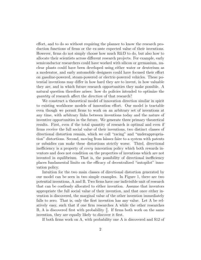
Intuition for the two main classes of directional distortion generated byour model can be seen in two simple examples. In Figure 1, there are twopotential inventions, A and B. Two firms have one indivisible unit of researchthat can be costlessly allocated to either invention. Assume that inventorsappropriate the full social value of their invention, and that once either in-vention is discovered, the marginal value of the other invention immediatelyfalls to zero. That is, only the first invention has any value. Let A be rel-atively easy, such that if one firm researches A while the other researchesB, A is discovered first with probability 3

4. If firms both work on the same

invention, they are equally likely to discover it first.If both firms work on A, with probability one A is discovered and $12 of

2

A B

Easy to invent,worth $12

Three times harder,worth $16

Figure 1: The racing distortion

value is created, and if both work on B, $16 is created. If one firm workson A and the other on B, with probability 3

4A is invented first, and with

probability 14

B is invented first, creating a total value of 34·$12+ 1

4·$16 = $13.

The efficient solution involves both firms working on B, creating $16 of value.However, working on B is not an equilibrium. A firm earns $8 in expectationwhen both work on B, but it earns 3

4· $12 = $9 from deviating and working

on A. The firm that deviates does not properly account for the fact thatwhen it makes a discovery, the rival firm can no longer earn any surplusby discovering the now-worthless alternative invention. Notice that this isprecisely the intuition of the racing distortion of classic patent race modelslike Loury (1979) in a directional context, substituting the extensive marginof which project to work on for the intensive margin of how hard to work,and the opportunity cost of foregone inventions for the cost of research effort.

Racing behavior is not the only way direction choice can induce ineffi-ciency. In Figure 2, again let there be two firms allocating one indivisibleunit of research each, and let there initially be two equally easy inventionsA and B. Since they are equally easy, the probability a given firm inventsfirst is 1

2regardless of what the other firm works on, hence there is no racing

distortion. In addition, assume that once A is invented, it becomes possiblefor each firm to work on a third invention, C. Further, assume that once Ais invented, the marginal value of B falls to zero, and once B is invented, themarginal value of both inventions A and C fall to zero.

The most social value, $12, is created when both firms work on A andthen on C. Each firm expects to earn $6 under this research plan, but thisis not an equilibrium. A firm that deviates by working on B instead ofA will finish first with probability 1

2, earning $10. If A is invented before

B, the deviating firm can still try to invent C at that point, earning 12·

$8 = $4 in expectation. The expected payoff of the deviation is 12· $10 +

12· $4 = $7, hence deviating is profitable. This example illustrates that

3

0

A B

C

Easy to invent,worth $4

As easy as A,worth $10

As easy as A,worth $8

Figure 2: The underappropriation distortion

inventors do not properly account for how their inventive effort today affectsthe nature and availability of socially valuable projects other firms mightinvent in the future. This is precisely the intuition of the underappropriationdistortion of sequential innovation models like Green and Scotchmer (1995)in a directional context, substituting distortion toward research lines wheresequential inventions are relatively unimportant for inefficient effort alongthe intensive margin in a single sequential research line.

Our formal model will show that if we abstract away from known distor-tions in the market for R&D — for instance, if the total quantity of researchis fixed at the socially optimal optimal level, if the research sector capturesthe full social value of their inventions, if researchers can be induced to workwithout agency problems, and if there is perfect knowledge among all firmsabout research opportunities today and in the future — then a competitiveresearch sector will nonetheless be inefficient because of a combination ofracing and underappropriation distortions. This dual distortion means thatpolicies like patents and prizes will not necessarily improve efficiency, unlikein models where laissez faire research effort is inefficient.

Consider first patents, which let an inventor today capture the value ofprojects tomorrow which build on her invention. Patents cause firms to in-ternalize the fact that their inventions today make future inventions easier orpossible in the first place, but they do not fix, and may make worse, the racingdistortion. Firms will be induced to race toward any invention which garnersan industry-pivotal patent, regardless of whether that particular technologylies on a research line which is easy to productively extend. Prize contestsare likewise problematic, as prizes for inventions exceeding a technological

4

threshold exacerbate racing behavior toward lower-value projects which arejust sufficient to garner the prize. Prizes given only to difficult technologi-cal achievements will push firms toward those types of projects, but if theoptimal projects are easy yet avoided because of underappropriation, such apolicy may simply make equilibrium directional distortion worse.

Note that patents and prize contests both condition inventor rewardssolely on the properties of realized inventions, and not on properties of un-realized alternative research projects in the same technological area. Indeed,this is an important virtue of these types of policies: they can be run “auto-matically” by a planner who is ignorant of anything except ex-post observablefeatures of inventions. However, when directional distortion is important,whether firms are deviating toward easy though potentially low-value inven-tions because of the racing distortion, or toward immediately lucrative yetpotentially difficult inventions because of the underappropriation distortion,depends on the properties of all inventions including those which are not ac-tually invented in equilibrium. Therefore, innovation policy which does notcondition on the properties of those unrealized potential inventions, proper-ties which may be very hard for the planner to observe, will be unable torestore directional efficiency across industries.

In the remainder of the paper, we develop the above intuition formally.In Section 1, we show how to construct planner-optimal and equilibrium dy-namic research allocation for an arbitrary set of inventions with unrestrictedlinkages in how earlier inventions affect the value or difficulty of future in-ventions. In Section 2, we show that, in this general model, equilibriumdirectional inefficiency is driven by a combination of racing and underappro-priation distortions qualitatively similar to those in the examples above. InSection 3, we show that laissez faire, patents of various strengths, and prizescannot be ranked in terms of welfare, and that every policy which rewardsinventors more than non-inventors and does not condition on the propertiesof off-equilibrium-path inventions cannot guarantee directional efficiency. Wediscuss four applications of the theory in Section 4. All proofs, and a numberof generalizations, are left to the appendices.

Our results differ from the existing literature in restricting attention tothe distortion between the planner and the firms when there are multipleprojects available at any time, and success on a project changes the natureof research targets available in the future.1 That is, we study inefficiency

1That firms may lack correct directional incentives in R&D is a longstanding worry,

5

in research lines. The distortions generated, and the relative advantages ofdifferent mitigating policies, do not depend in any way on information ex-ternalities (as in bandit models like Keller and Oldale (2003) and Chatterjeeand Evans (2004)), changing preferences (Acemoglu (2011)), changing factorprices (Kennedy (1964), Samuelson (1965), Acemoglu (2002)), simultaneousdiscovery (Dasgupta and Maskin (1987)), heterogeneity across firms in size orinternal organization (Holmstrom (1989), Aghion and Tirole (1994)) or dif-ferences in researcher desire for autonomy (Aghion, Dewatripont and Stein(2008)).2 Our distortions arise even if the total quantity of research is op-timal, and even if there is no gap between the social and private return toindividual inventions.3

Directional inefficiency may be of particular importance due to limitson the ability of policy to affect the rate of innovation. Even when basicresearch has a high marginal return, both privately and socially, the returnto government-sponsored R&D is often much more limited (e.g., David, Halland Toole (2000), Lerner (1999)). This result is partially due to crowding out:the supply of trained scientists is essentially fixed in the short run (Goolsbee(1998)). If crowding out limits how planners can affect the rate of inventiveactivity, affecting R&D direction may be a first-order effect of governmentpolicy. Our results suggest fundamental limits on existing policy levers in

however. Nelson (1983) argues that “[i]t is not so much that private expenditures will betoo little in the absence of government assistance. The difficulties lie rather in the factthat the market, left to itself, is unlikely to spawn an appropriate portfolio of projects.”

2A discrete version of Acemoglu’s 2011 result can be seen in our framework. He allowsconsumer preferences over technology lines to change. Patents are of finite length, so withsome probability work on a line consumers do not value may not be worth anything untilafter the patent expires, and hence firms exert too much effort on lines where rents canbe accrued in the near future. In our model, the possibility of preferences changing justfeeds into the continuation value following some invention; firms undervalue social payoffsthat accrue through the continuation value rather than immediately, since part of thatcontinuation is captured by competitors.

3The most similar result we are aware of, though in the context of a structural en-dogenous growth model, is Akcigit, Hanley and Serrano-Velarde (2013), which suggestslike our model that “neutral subsidies” like R&D tax credits operate by increasing thetotal amount of R&D without correcting the distortion toward applied research. A math-ematically similar model to ours of direction choice applied to the context of competingpatent races appears in a new working paper by Hopenhayn and Squintani (2016). In theirmodel, firms in the analogue of our laissez faire equilibrium work first on relatively easyinventions even when working in this “hot” area is socially undesirable. The fundamentalreason is very similar to the racing distortion in our model.

6

restoring directional efficiency.

1 The Model

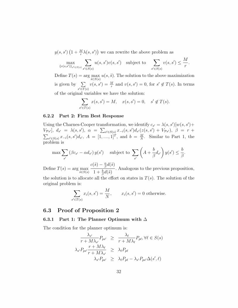
Consider a finite set of states Ω, where s ∈ Ω represents a level of technology,or a collection of existing inventions. Transitions between states are associ-ated with two parameters λ, π, where we define λ : Ω × Ω → R+ as thesimplicity to transition between any two states, and π : Ω× Ω→ R+ as theincremental immediate social payoff from a transition. When λ(s, s′) = 0,state s′ cannot be reached with one invention from state s. For each states ∈ Ω, the set S(s) ⊆ Ω represents all the states such that λ(s, s′) > 0. Werefer to the initial state of technology as s0.

Definition 1. An invention graph is represented by the triplet Ω, λ, π de-scribing all potential states Ω of knowledge in a technological area, the sim-plicity λ : Ω × Ω → R+ of transitioning between them, and the immediatesocial payoff π : Ω× Ω→ R+ from such a transition.

The invention graph is common knowledge and all discoveries and inven-tive effort are publicly observed.4

As an example, consider the case of three inventions represented by theinvention graph in Figure 3. In this example, the possible states of technologyare given by Ω = s0, 1, 2, 1, 2, 1, 3, 1, 2, 3. The transition andpayoffs are given by the parameters (λk, πk)9

k=1. There is an arrow betweenstates s and s′ if and only if λ(s, s′) > 0. In state s0, only inventions 1 or 2can be discovered in one step, and once either 1 or 2 have been discovered,research on invention 3 can begin.

4Relaxing the assumption that all future parameter values are commonly known toan assumption that only the distribution of parameter values in future states is knownwill not change our qualitative results. With perfect information, this assumption wouldmerely change the expected continuation value following any invention, which will appearas an arbitrary parameter in Proposition 2. Indeed, if inventions today publicly resolveuncertainty about future parameter values, then inventions potentially create informationuseful to all parties, generating a positive externality. Thus, inventions which create alot of useful information will be undersupplied by firms in equilibrium. We will not focuson these types of information transmission externalities in the remainder of this paper, asthey are well-known from the multi-armed bandit literature (e.g., Keller, Rady and Cripps(2005)).

7

Our model allows state contingent payoffs and simplicities. In Figure3, λ2 and λ4 are unrestricted, meaning that the discovery of invention 1may increase (λ2 > λ4), decrease (λ2 < λ4), or keep constant (λ2 = λ4) thedifficulty of discovering invention 2. Similarly, π2 and π4 can differ, capturingsubstitutability or complementarity between inventions 1 and 2.

In the remainder of the paper, we refer abstractly to states without ref-erence to the exact bundle of inventions a particular state embodies, callingstates s′ ∈ S(s) projects, research targets, or inventions.

s0

1 2

1, 21, 3 2, 3

1, 2, 3

(λ1, π1) (λ2, π2)

(λ3, π3) (λ4, π4) (λ5, π5) (λ6, π6)

(λ7, π7)(λ8, π8) (λ9, π9)

Figure 3: A simple invention graph.

1.1 Production Technology

There are N risk-neutral firms each endowed with MN

units of research, whereM represents the total measure of researchers in society. Let xi(s, s

′) ≤ MN

be the flow amount of research allocated by firm i toward state s′ ∈ S(s)when the current state is s, and let x(s, s′) =

∑i xi(s, s

′) be the aggregateflow amount of research toward state s′.5 Research is costless, so the problem

5Although time is continuous in our model, optimal and equilibrium strategies willbe constant between state transitions, hence we omit time subscripts. Intuitively, noinformation is revealed and no changes in the strategy set or payoffs occur between statetransitions.

8

is one of pure allocation of research resources.As in patent race models, the probability of discovering s′ given xi(s, s

′)in a given interval of time is determined by the exponential distribution,with hazard rates λ(s, s′)xi(s, s

′) linear in effort, independent across firms,and independent across research lines within any firm.6 Therefore, the un-conditional probability of a transition from s to s′ in an interval of time τ isgiven by 1− exp(−λ(s, s′)x(s, s′)τ).

In the remainder of the paper, we will omit some indexes for ease ofnotation, denoting xi(s, s

′) simply as xis′ , and likewise for similar variables,when it is clear that s′ ∈ S(s).

1.2 Planner Problem

Since the invention hazard rates are linear and independent across firms,a risk-neutral social planner needs only decide how to allocate all M unitsof research across projects. The expected discounted value of the inventiongraph for the planner at state s ∈ Ω is defined recursively as

Vps = max∑s′∈S(s) xs′=M,

xs′≥0, ∀s′∈S(s)

∫ ∞0

e−rte−

∑s′∈S(s)

λs′xs′ ·t ∑s′∈S(s)

λs′xs′ · (πs′ + Vps′)dt

That is, after reaching state s, the planner chooses the allocation x =(xs′)s′∈S(s) to maximize the future discounted payoff: the integral with re-

spect to time of the probability that no invention has occurred (e−∑s′∈S(s) λs′xs′ t),

times the immediate hazard rate of each research line (λs′xs′), times the dis-counted (e−rt) payoff summed over all possible inventions inclusive of con-tinuation value from a discovery along that line (πs′ + Vps′). Simplifyingthe expression above, the social planner problem is to solve the recursivemaximization problem:

Vps = max∑s′∈S(s) xs′=1,

xs′≥0, ∀s′∈S(s)

∑s′∈S(s)

Mλs′xs′ [πs′ + Vps′ ]

r +∑

s′∈S(s)

Mλs′xs′

6In the Online Appendix, we generalize to a hazard rate that is concave or convex inxi(s, s

′). There are technical difficulties with this objective function (in particular, non-pseudoconcavity) which do not appear, for example, in one-shot models like Reinganum(1981), but our main qualitative results do not change.

9

1.3 Firm Problem

Let policy P determine the transfers received by firms following an invention.In particular, P specifies transfer w(s, s′) received by inventors and transferz(s, s′) received by noninventors following any invention. At each state s ∈ Ω,the equilibrium continuation value for firm i following a transition to s′ ∈S(s) given policy P is denoted ViPs′ .

7 The firm problem is to allocate its MN

units of research among the projects s′ ∈ S(s), conditional on other firms’allocations and the policy rule. Once any firm discovers some inventions′ ∈ S, all firms reallocate effort across the new set of potential researchtargets S(s′).

Denote a−is′ =∑j 6=i

xjs′ as the total research allocated towards invention

s′ by firms other than i. Given the strategies of rivals a−i = (a−is′)s′∈S(s) andthe policy rule P , the expected discounted value of firm i at state s can bewritten recursively as

ViPs|a = max∑s′∈S(s)

xis′=MN ,

xis′≥0, ∀s′∈S(s)

∫ ∞0

e−rt−

∑s′∈S(s)

(a−is′+xis′ )λs′ t∑s′∈S(s)

λs′ [xis′(ws′+ViPs′)+a−is′(zs′+ViPs′)]dt

The strategy of each player depends on the current state, the equilib-rium continuation value, and the current allocation of effort of rival firms.Simplifying this expression, firms solve:

ViPs|a = max∑s′ xis′=

MN,

xis′≥0, ∀s′∈S(s)

∑s′∈S(s)

λs′ [xis′(ws′ + ViPs′) + a−is′(zs′ + ViPs′)]

r +∑

s′∈S(s)

λs′(xis′ + a−is′)

1.4 Common Transfer Policies

We permit general transfer policies P , but four classes will be of specialrelevance: laissez faire, patents, neutral prizes, and information-constrainedpolicies. Laissez faire gives inventors the immediate social payoff of theirinvention, but permits all firms to equally build on that invention.

Definition 2. The transfer policy PLF is laissez faire if inventing firmsreceive the full immediate social payoff of their invention, i.e. w(s, s′) =

7Forcing the continuation value to be identical for inventing and noninventing firms iswithout loss of generality since w and z are unrestricted.

10

π(s, s′), and if noninventing firms receive no immediate transfer following aninvention but are equally able to build on today’s invention (z(s, s′) = 0).8

We model patents as a tractable reduced form of a licensing game. Letparameter γ ∈ [0, 1] indicates what fraction of the total continuation valuefollowing any invention non-inventors have to cumulatively pay to the inven-tor.9 If γ = 1, patents are so strong that the inventor of s′ is immediatelygranted the entire discounted surplus generated by their invention includingsurplus from any invention which builds on it in the future. If γ = 0, patentsare equivalent to laissez faire.

Definition 3. The transfer policy Pγ involves patents if inventing firmsreceive transfers w(s, s′) = π(s, s′) + (N − 1)γViPγs′ and noninventors pay(receive a negative transfer) z(s, s′) = −γViPγs′, for γ ∈ [0, 1].

Prizes and contests are another common innovation inducement scheme.Let a neutral prize q in state s be a lump sum awarded to the inventor of anyproject s′ ∈ S(s), in addition to the immediate payoff πs′ and continuationvalue ViPs′ . Many real-world prizes share this structure, where any inventionachieving a given technological threshold is rewarded with a constant prize.For example, the Netflix contest awarded $1M to the firm that “substantiallyimproves the accuracy of predictions about how much someone is going toenjoy a movie based on their movie preferences.” If q is interpreted morebroadly as a form of utility for an inventor, then it may also represent credit inthe Mertonian sense; merely passing a technological threshold, regardless ofeconomic significance, is the cutoff upon which scientific credit is distributed.

Definition 4. The transfer policy Pq involves neutral prizes in state s ifthe first firm to successfully invent any invention in state s receives transfersw(s, s′) = π(s, s′) + q and noninventors receive transfer z(s, s′) = 0.

Patents, neutral prizes and laissez faire are all policies which do not con-dition transfers w(s, s′) and z(s, s′) on off-equilibrium-path parameters: the

8The assumption that firms earn the full social surplus under laissez faire from eachinvention is not critical for our results. Under the laissez faire policy, since π enters the firmvalue function linearly, a straightforward induction argument shows that if all immediatefirm payoffs π are scaled by σ > 0, the firm problem is unchanged. Only the relative valuesof immediate payoffs affect the choice of direction.

9Specifying patent payments in this way allows us to retain the earlier assumption that,following these side payments, all firms receive equal continuation values.

11

transfer following the invention s′ does not depend on the parameters ofprojects ` 6= s′ ∈ S(s). In this sense, these policies all lie in a class wecall information-constrained, meaning any policy where transfers followingan invention do not condition on the parameters of inventions which are notinvented in equilibrium. An example of a policy which is not information-constrained is an NIH funding panel, which explicitly takes into accountthe value and challenge of alternative projects when choosing which projectsshould receive funding.

Definition 5. A transfer policy P is information-constrained if transfersw(s, s′) and z(s, s′) do not condition on the parameters of inventions ` 6= s′.

2 Planner Optimum and Firm Equilibrium

The planner and firm problems both involve choosing vectors of effort acrossan arbitrarily large number of projects. In principle, then, comparing theefficiency of the optimal and equilibrium allocations involves comparing thewelfare induced by two arbitrary vectors describing aggregate effort in everystate. Worse, neither the planner maximand nor firm equilibrium have an-alytically tractable first order conditions, hence a mathematical workaroundis required to make non-numerical statements about efficient and inefficientdirectional policy.

Although the objective function for the planner and the firms is non-linear in the research allocation, both problems are linear fractionals withlinear inequality constraints. The Charnes-Cooper transformation (Charnesand Cooper (1962)) converts programs of this type into analytically tractablelinear programs. These linear programs have corner solutions, where fulleffort is optimally exerted on a single project at a single time, and the cornersolutions can be stated in terms of the maxima of simple indices. The problemof directional efficiency is therefore tractable. In any state, the planner willdirect all researchers to work on a single project, and knowing which projectis optimal simply involves checking which invention maximizes a particularindex derived from the linear program solution. A firm equilibrium mayinvolve firms all working on the same project or on different projects, butcritically the existence of a socially optimal firm equilibrium requires onlyknowing whether there exists an equilibrium where all firms exert full efforton the planner’s preferred project. This can again be checked using a similarsimple index.

12

Define r = Nr+M(N−1)λs′ , which corresponds to a virtual discount ratefor competing firms, and denote by Θ the expected discounted continuationvalue for firm i when firm i does not exert any effort until the next inventionis completed by some firm:

Θ =

∑s′∈S a−is′λs′(zs′ + ViPs′)

r +∑

s′∈S(s) a−is′λs′.

Denote the immediate payoff plus the continuation value as PiPs′ = ws′+ViPs′for an inventing firm i under policy P and Pps′ = πs′ + Vps′ for the planner.We refer to λs′πs′ as the flow immediate social payoff, λs′Vps′ as the flowsocial continuation value, λs′Pps′ as the flow total social payoff, and the timebetween any two inventions as a “period.”

Proposition 1. In state s ∈ Ω:

1. The planner optimum puts all research effort toward states s′ ∈ S(s)which maximize the index

Mλs′

r +Mλs′Pps′

2. The best response of firm i given rival effort a−i and policy P is todistribute all of its effort among states s′ ∈ S(s) which maximize theindex

Mλs′

r +Mλs′(PiPs′ −Θ)

The firm’s best response index differs from the planner’s in three ways:transfers to firms inclusive of continuation value may differ from the totalsocial payoff (Pps′ 6= PiPs′); firms maximize payoffs only marginal to the Θwhich is earned from doing nothing in the current state; and firms effectivelydiscount at a different rate from the planner since their research decisiontoday only has a partial effect on the eventual time the next invention insociety is completed, and hence the time at which all firms can begin workon new projects (r 6= r).

The planner index generically has a unique maximum. It may seem sur-prising that the planner does not mix across projects, but generating an un-derlying reason for R&D diversity is a tricky modeling problem, frequentlymisunderstood in informal discussion. The intuition that a diverse research

13

agenda provides “more lottery tickets” is false in the absence of decreasingreturns to scale in the research production function, since simultaneous di-versified research with any constant returns to scale can be replicated bysequentially exploring projects, with the benefit that sequential explorationallows a high level of effort to be exerted first on projects which are believedto be more valuable. It can be shown in a variant of our main model that un-certainty about parameter values, switching costs, asymmetry across firms,or even low levels of decreasing returns to scale do not necessarily lead aplanner to work on multiple projects at a time.10

2.1 Efficiency of the Firm Equilibrium

The planner optimum generically involves full effort in each state on a singleinvention s′. From the best response characterization in Proposition 1, we canconstruct firm equilibria, calling them efficient if there exists any equilibriumwhere firms allocate their research in the planner optimal way. We restrict toMarkov perfect stationary equilibria throughout to rule out equilibria wherefirms collude and punish each other across states.11

Definition 6. The firm equilibria in state s are efficient under policy P ifthere exists a Markov perfect stationary equilibrium involving full effort fromall firms toward planner optimal s′ ∈ S(s).

In the next proposition, we characterize the trade-off faced by firm whendeviating from the efficient research path. First, define

∆(s′, `) =M(λ` − λs′)r +Mλs′

=

1

r +Mλs′− 1

r +Mλ`1

r +Mλ`

which measures the relative difference of the value of $1 forever with discountrates indexed by λs′ and λ`.

Proposition 2. Let the current state be s.

10See Online Appendices B and C for details.11The Online Appendix discusses the existence, multiplicity, and potential asymmetry

of firm equilibria.

14

1. Project s′ is planner optimal if and only if, for all ` ∈ S(s)

λs′Ps′ ≥ λ`P` − λs′Ps′∆(s′, `)

2. Project s′ is a firm equilibrium if and only if, for all ` ∈ S(s)

λs′Ps′ ≥ λ`P` − λs′Ps′∆(s′, `) +D1(s′, `) +D2(s′, `) +D3(s′, `),

where

D1(s′, `) = λs′(Pps′ − (ws′ + ViPs′))− λ`(Pp` − (w` + ViP`))

D2(s′, `) =

(N − 1

N

)∆(s′, `)λs′Pps′

D3(s′, `) =1

N∆(s′, `)λs′(Pps′ − (ws′ + (N − 1)zs′ +NViPs′))

The first part of Proposition 2 simply restates the planner optimum inProposition 1 in terms of discounted flow payoffs. The second part of Propo-sition 2 fully decomposes the source of inefficiency in the firm equilibriuminto three parts.

D1(s′, `), the underappropriation distortion, is positive when a firm devi-ating from project s′ to project ` receives a higher portion of the total socialvalue of the invention. D2(s′, `), the racing distortion, captures the incentiveto deviate toward easier projects because firms do not account for how theireffort affects the probability other firms succeed with alternative projects ina given period of time. D3(s′, `), the industry payoff distortion, is zero whenthe total payoff to all firms under policy P is equal to the total social payoffof each invention. When that condition does not hold, the racing externalityis either minimized or exacerbated.12 If s′ is the planner optimum, any policyP such that D1(s′, `) +D2(s′, `) +D3(s′, `) ≤ 0, for all ` ∈ S(s), implementsthe efficient direction.

The decomposition in Proposition 2 is perhaps surprising. Research byfirms affects what projects other firms can work on tomorrow, when these fu-ture projects become available, the probability a given firm actually inventsthe project it is currently working on, and so on, and yet any innovationpolicy can generate inefficiency in only three ways: either firms are overin-centivized to race toward projects easier than the planner preferred ones; or

12Recall that ∆(s′, `) > 0 when invention ` is easier than s′.

15

inventing firms do not appropriate a sufficiently large share of the surplustheir inventions generate; or researching firms overall receive a different shareof the social surplus of invention depending on which research lines are pur-sued. These are the fundamental ways competition in the resaerch sector cangenerate directional efficiency, as they can exist even when the total aggre-gate amount of research is fixed at the (unmodeled) socially optimal level,and even though our model deliberately shuts down any distortions whichlead to inefficiency with a single private firm.13

Consider, for example, the laissez faire policy, which generates transfersto the inventor w(s, s′) = π(s, s′) and to noninventors z(s, s′) = 0. If thefirm equilibrium in all future states is efficient, then by induction the firm

continuation value under laissez faire is ViPs′ =Vps′

N; each firm collects, in

expectation, an equal share of the social continuation value. In this case,D3 = 0 because total industry transfers are exactly the total social payoff.Since inventors only receive a 1

Nshare of the social continuation value, and

firms are overincentivized to work on relatively easy projects, the underap-propriation distortion D1 and racing distortion D2 distort behavior.

Corollary 1. When firms research efficiently in all future states, under thelaissez faire innovation policy PLF :

D1(s′, `) =

(N − 1

N

)(λs′Vs′−λ`V`), D2(s′, `) =

(N − 1

N

)λs′∆(s′, `)Pps′ , D3(s′, `) = 0

The firm equilibrium condition in Proposition 2 collapses to:

λs′Ps′ ≥ λ`P` − λs′Ps′∆(s′, `) + (N − 1)(λ`π` − λs′πs′).

Corollary 1 says that under laissez faire, firms are incentivized to deviatetoward projects with high immediate flow payoffs λπ. These projects maybe easier than the planner optimum (λ` > λs′), or have a higher immediatepayoff (π` > πs′), or both. The magnitude of the distortion is increasingin N , and hence Proposition 3 shows that sufficient fragmentation of theresearch sector guarantees inefficiency unless the planner optimal project ina given state has higher flow immediate payoff than any potential deviation.

Proposition 3. Let the firm equilibrium in future states be efficient.

13It is trivial to note that when N = 1, invention is always directionally efficient, as asingle private sector firm in our model will behave identically to a social planner.

16

1. If planner-optimal s′ is not a laissez faire equilibrium when there areN firms, s′ is still not an equilibrium for any N ≥ N .

2. If the planner optimal invention does not maximize λsπs,∀s ∈ S(s),then there exists a level N∗ of fragmentation in the research sectorsuch that if N ≥ N∗, the laissez faire firm equilibrium is inefficient.

Not every type of invention graph leads to laissez faire inefficiency. Inthe Online Appendix, we prove that directional inefficiency requires both theexistence of multiple research targets in some states, and some form of statedependence linking invention today to inventive opportunities tomorrow. Ifthere are multiple research targets, but invention today does not change thesocial value or simplicity of the remaining targets, the laissez faire equilib-rium is efficient. Since there is no benefit in continuation value from avoidingprojects with high flow immediate payoff, and the future is discounted, theplanner will work first on projects with maximal λπ, hence by Corollary 1the firms will not deviate. However, once a single element of state depen-dence is introduced - for example, an invention which requires a precursor,or an invention which is made easier by complementary inventions, or aninvention whose value is reduced once a substitute exists - the laissez fairefirm equilibrium is no longer efficient in general.

3 General Policy Solutions to Directional In-

efficiency

In the previous section, we saw that laissez faire is not directionally efficient.In this section, we show that prize contests, and patents of various strengths,also do not induce efficient equilibria, that patents, prizes and laissez faire caneach be more efficient than the others, and that any efficient invention graphmust either condition on off-equilibrium-path parameters of the inventiongraph or reward noninventors as highly as inventors. That is, information-constrained policies, whose transfers are simple functions of on-equilibrium-path observables, are insufficient when it comes to directional efficiency.

3.1 Neutral Prizes

Recall that the neutral prize policy Pq awards a lump sum q to the inventorof any project s′ ∈ S(s)

17

Corollary 2. In state s, under neutral prize policy Pq, total distortions are

D∗NP (s′, `) = D∗LF (s′, `) +∆(s′, `)

Nqr

where D∗LF (s′, `) is the equilibrium distortion in Proposition 2 under laissezfaire.

Neutral prizes of any size do not guarantee efficiency, and indeed cangenerate an inefficient outcome even when laissez faire is efficient. Notethat neutral prizes still generate the underappropriation distortion of laissezfaire, since firms only collect a portion of the social continuation value oftheir inventions. In addition, since ∆(s′, `) > 0 only for projects ` thatare easier than the planner optimal project s′, neutral prizes exacerbate theracing distortion toward projects that are easier than the planner optimum.Intuitively, a fixed prize q increases the payoff, in percentage terms, of low-value projects more than high-value projects. Therefore, prizes can onlymake firms more likely to work on lower-value yet easier projects than thelaissez faire equilibrium, as they race to finish inventions which are easy yetjust sufficient to garner the prize.

In practice, then, large prizes will cause firms to race toward inventionswhich can be completed more quickly because the incentive from winningthe prize overwhelms the incentive of developing a potentially more difficulttechnology that is easier for the inventor to build on in the future. If qrepresents the value to an inventor of Mertonian credit for a breakthrough,the exact same distortion arises. However, if the prize designer believes thatfirms are working on inefficiently hard projects because the inventor of thoseprojects can capture a large share of the total value of a research line—e.g.,projects that can be kept secret—then prizes may be effective in reducing thattype of directional inefficiency. These directional distortions must be tradedoff against whatever increase in effort, unmodeled here, a prize designer hopesto generate toward research in a given technological area.

3.2 Patents

Patents are thought to play an important role when sequential innovationis critical, since patent rights limit double marginalization when inventionsbuild on each other (Green and Scotchmer (1995)). When multiple researchlines can be pursued, however, patents can distort ex-ante incentives even

18

when they ameliorate ex-post double marginalization problems. The grantof a broad patent which covers substitutes and downstream inventions cancause a race among upstream inventors to develop relatively easy yet sociallyinefficient early-stage inventions in order to obtain this broad patent.

Recall that under the patent policy Pγ, inventors receive transfers w(s, s′) =π(s, s′) + (N − 1)γViPs′ and noninventors pay z(s, s′) = −γViPs′ , where γ ∈[0, 1] represents the fraction of the continuation value following a patentedinvention which is collected by the initial inventor.

Corollary 3. Under patent policy Pγ, distortions are

D∗Pγ (s′, `) = D∗LF (s′, `) + γ(N − 1)(λ`VPγ` − λs′ViPγs′) + V(γ),

where

V(γ) = (1 + ∆(s′, `))λs′(ViPLF s′ − ViPγs′)− λ`(ViPLF ` − ViPγ`)

Suppose that invention in all future states is efficient (ViPLF s = ViPγs =VpsN,∀s), hence V(γ) = 0. In this case, patents of maximal strength γ = 1

exactly cancel out the laissez faire underappropriation distortion D1(s′, `), asmight be expected. Patents, however, do not affect the laissez faire racingdistortion D3(s′, s). If the underappropriation distortion under laissez faireis helping counteract the racing distortion—e.g., if firms are not deviatingtoward an inefficient easy project under laissez faire because they would onlycapture a small portion of the total social value of that invention—then in-creasing the strength of patents can actually make directional inefficiencyworse. In practical terms, with strong patents, firms may avoid hard inven-tions with large payoffs because racing to invent something easier gives thema claim over the value of future discoveries, including some substitutes whichmay have been potential research targets from the start.

An immediate implication of the previous two corollaries is that thereexist invention graphs for which patents of various strengths, neutral prizes,and laissez-faire each dominate the others in terms of social welfare. We givenumerical examples in Online Appendix B.

3.3 Directional Efficiency With Information ConstrainedPolicy

Patents and prizes both condition on very little information: the incentivesthey provide to firms depend only on the parameters of on-equilibrium-path

19

inventions, and hence can operate “automatically.” Both policies were shownto have difficulty simultaneously limiting racing behavior while still causingfirms to care sufficiently much about the social continuation value their re-search generates. This finding raises the question: does there exist any policywhich can generate directional inefficiency without conditioning on the pa-rameters of off-path inventions?

Recall from Definition 5, in section 1.3, that a policy is information-constrained if transfers do not condition on the parameters of inventionswhich are not ever invented in equilibrium. We show in Proposition 4 thatany information-constrained policy which is always efficient must reward in-venting firms at least as much as non-inventing firms. That is to say, ifinventors are to be rewarded more than non-inventors, the dual nature ofdirectional distortions, coming both from racing behavior and underappro-priation, cannot be wholly corrected by any information-constrained policy.

Proposition 4. Let transfer policy P be information-constrained.

1. If the payoff of inventors and non-inventors can be equalized, the information-constrained policy w(s, s′) = z(s, s′) = απ(s, s′),∀α ≥ 0 implementsefficiency on any invention graph.

2. If the payoff (inclusive of continuation value) for inventors must bestrictly higher than that of non-inventors, then there exists no information-constrained policy which is efficient for all invention graphs.

The first part of Proposition 4 is trivial: since we have shut down allnondirectional distortions in our model, if the payoff to inventors and non-inventors is identical, there is no benefit for any firm from taking any actionthat lowers the cumulative payoff to all firms. If the cumulative payoff to allfirms is maximized along the efficient path, then direction will not be dis-torted in equilibrium.14 For many reasons aside from directional efficiency,however, we may wish to rule out policies that reward inventors and non-inventors equally, the most obvious one being that getting the total rate ofeffort to the optimal level may require rewarding inventors in some way.

The second part of the Proposition 4 shows that any efficient policy whichgives larger rewards to inventors than non-inventors must condition on the

14Other efficient policies like “paying firms only if they invent along the socially optimalresearch line” require the mechanism to condition on the full vector of simplicities in orderto compute the optimal direction.

20

parameters of off-equilibrium-path inventions. Therefore, the result shouldbe read as an impossibility result concerning uniform, non-targeted policies,which condition on ex-post public features of an invention to generate correctdirectional incentives, rather than as an implementation result in the formalsense of the term in mechanism design.

The intuition of Proposition 4, as can be seen in the formal proof, isas follows. Consider any invention graph with states where the planner isindifferent between two inventions, and where the indifference may result be-cause an invention s′ is harder or easier than an alternative `. Since w > zby assumption, if the relative total transfer to inventors of two inventionsis equal to the relative total social payoffs, so that there is no underappro-priation, then firms will race toward easier inventions. An arbitrarily smallchange in the simplicity or payoff of the off-equilibrium-path invention willmake the planner optimum unique, and hence the proposed transfer policywill be inefficient. On the other hand, whether transfers should be biasedtoward s′ or ` depends on which one is easier and inducing racing as a re-sult, a comparative question that necessarily depends on the simplicity of theoff-equilibrium-path invention. This result does not require any unusual in-vention parameters or interactions: all that is required is for the planner to bepotentially unsure in some states whether the racing and underappropriationdistortion is dominant.15

Empirically, many common innovation policies are information-constrained,and hence the inefficiency result in Part 2 binds. Governments appear to de-sire “neutral policies” since they impose less cost in terms of informationgathering and less scope for political considerations to factor into the rewardsystem for inventors. Whatever the reason, our result suggests that avoidingtargeted policies has a cost in terms of efficiency. Note that our definition of“information-constrained” allows more planner information than is usuallyassumed when justifying policies like patents, since we permit conditioning

15The reader may wonder whether certain types of invention graphs are efficient underlaissez faire or under a particular policy: that is, is the inefficiency result driven by “weird”invention graphs, or is directional inefficiency a generic property? It is trivial to constructclasses of invention graphs where simple policies generate efficiency. For example, if inevery state there is one invention that is both easier and more immediately lucrative thanany other, laissez faire will be efficient. However, both the nature of the inefficiency proof,and results proved in the Online Appendix, suggest to us that directional inefficiencyoccurs broadly. In particular, a single element of state dependence, where the nature ofinventive opportunity tomorrow depends on what is invented (or not invented) today, issufficient to construct graphs where laissez faire policy is inefficient.

21

policy on the full social value, including continuation value, of all inventionswhen setting transfers.

4 Applications and Implications

Though our primary results are theoretical, the model is general enough toapply to a broad set of policy problems, of which we consider four. First,competition among innovators can cause firms to work on projects that areeither more radical or more incremental than those preferred by the socialplanner. Second, patent pools or research joint ventures can play a role inreducing directional distortion in addition to their role in limiting holdupwhich is well-known in the existing literature. Third, when trade expansionsenlarge the size of the market, the endogenous entry of additional firms willdistort directional incentives. Fourth, the breadth of “pioneer patents”, oftendetermined ex-post in the courts, ought to account for the potential of ex-ante distortion.

4.1 Incremental Steps versus Large Steps

Proposition 5 shows that, perhaps counterintuitively, firms in competitiveequilibrium may work on inventions that are either too incremental or tooradical.

Proposition 5. Let an invention graph contain an incremental line with twosequential inventions 1 and 3, and a radical invention with a single invention2. Assume that the radical project is harder than either of the incrementalsteps (λ2 > maxλ1, λ3), that the radical invention payoff exceeds the totalpayoff of the incremental line (π2 > π1 +π3), and that once either the radicalinvention or the incremental line have been invented, the value of the otherline falls to zero.

1. If the planner is indifferent between the incremental line and the radicalline then the incremental line (radical line) is a laissez faire equilibriumif and only if λ1π1 ≥ λ2π2 (λ2π2 ≥ λ1π1).

2. There is an open set of parameters where the radical (incremental) lineis strictly preferred by the planner yet the radical (incremental) line isnot a laissez faire equilibrium.

22

When λ1π1 ≥ λ2π2, the racing distortion is stronger than the underap-propriation distortion: competitive pressure to finish some project quicklypushes firms off the difficult radical invention 2, leading them to work onincremental project 1 even though they will only capture a fraction of thevalue of the follow-on invention 3. On the other hand, if λ2π2 ≥ λ1π1, theunderappropriation externality is stronger: firms work on the radical inven-tion because although the incremental first step is easy, inventing firms mustin expectation share the continuation value generated once 3 is eventuallyinvented. Note also from Corollary 3 that under patents of maximal strengthγ = 1, only racing behavior distorts the firm equilibrium. Therefore, contraryto intuition, innovation will be excessively incremental in technological areaswhere patents are de facto effective in allowing originating firms to accruemost of the rents from follow-on innovation.

Essentially, if rivals are trying to invent a very difficult, very valuable newinvention, a firm can instead shift to a less valuable substitute research linewhere the initial steps are not that challenging. Since the initial steps arenot that hard, it is likely the firm will get the patent before its rivals makethe radical discovery, and hence even though the incremental line offers a lessvaluable industry, it offers the firm a high probability of holding an industry-controlling patent. The usual intuition that patents are necessary for radicalinvention is based on the idea that, in the absence of patents, firms will notcapture enough of the social value ex-post of their invention to justify a largeresearch investment. A directional model, on the other hand, clarifies thatstrong patents also encourage inefficient ex-ante racing for critical patentswhich may very well be incremental in nature.

4.2 Patent Pools

Patent pools and research joint venture cross-licensing agreements, madein advance of R&D investments, are common in many industries and theirpotential welfare-enhancing role in solving hold-up problems is well-known(Lerner and Tirole (2004), Denicolo (2002)). Our main result suggests analternative welfare-enhancing role for patent pools: reducing directional dis-tortion. The socially optimal inventions in an industry like semiconductorsmight reasonably be known better by private sector firms than the planner,or for political economy reasons the planner may not want to be seen dif-ferentially incentivizing specific inventions. Firms would prefer to committo innovating only along the optimal research line, but as we have shown,

23

research on these inventions is not generally a laissez faire equilibrium, hencesuch a commitment must be binding if the firms are to avoid deviating.

Patent pools serve this commitment role. From Proposition 4, if thepayoff to inventing firms and non-inventing firms is identical, then there isno directional inefficiency. A pool that involves the R&D intensive firmsin an industry committing to share revenue from the stream of inventionsthat follow will generate first-best directional efficiency even if there is noability to commit to precisely which type of innovation will be funded byeach firm, and even if the pool organizer does not know which inventions liealong the planner-optimal research line. We completely abstract away fromdeadweight loss generated either in the product market or in the technol-ogy licensing market, and so answering questions about the exact welfareimplication of patent pools is beyond the bounds of our model as currentlyconstructed. That said, the role of patent pools, research joint venturesand standard setting in generating an efficient industry research portfolioappears understudied: organizations like SEMATECH (Irwin and Klenow(1996)) rather explicitly set the goal of coordinating industry research onparticular research lines, rather than just hoping to reduce licensing frictionsex-post, or free riding ex-ante.

4.3 Trade Expansion and the Direction of Innovation

Trade is often considered a net positive for innovation, both because it ex-pands the size of the markets, and because it assists in the diffusion of knowl-edge (e.g., Bloom, Draca and van Reenen (2015)). However, trade can beproblematic if it distorts the direction of innovation. Consider a version ofour base model where the number of firms is endogenous, retaining the as-sumption that the total measure of science in society M is fixed.16 Firms areassumed to pay a fixed cost F at time 0 to enter, and no entry or exit occursafter that date. If entry decisions are made simultaneously, then the numberof firms is the largest integer such that ViP(s0, N) ≥ F . That is, firms enteras long as their expected discounted profits exceed the fixed cost.

Assume that an expansion of trade increases the immediate social payoffπ to all inventions by a constant factor ζ. From Proposition 1 and Footnote8, we know that holding the number of firms N constant, neither the planner

16For example, an expansion in North-South trade may expand the potential productmarket without changing the size of the research sector.

24

optimal projects nor the firm equilibria change. However, the value of theinvention graph for each firm increases to ζViP(s0, N), which is equivalent toa reduction in the entry cost to F

ζwhen calculating the number of firms who

enter in the long-run equilibrium. Thus, an expansion of trade implies thatthe equilibrium number of firms also increases.

The following proposition shows that a large expansion in the size of themarket, caused by trade, eventually causes so much entry in the R&D spacethat it distorts the direction of invention away from the planner optimum.

Proposition 6. Assume that prior to an expansion of trade, when ζ = 1,the direction of invention is efficient. Suppose there exists s ∈ Ω such thatthe planner optimal project is s′ ∈ S(s) and λs′πs′ < λsπs for some s ∈ S(s).Then, there exists an expansion of trade ζ > 1 such that the direction ofinvention is inefficient.

That an increase in the size of the product market can cause an increasein the number of producing firms under constant returns to scale is intuitive.The idea that increased competition among R&D performing firms followinga decrease in trade barriers can force firms to switch their research towardprojects which are either more immediately lucrative or quicker to completeis a complaint that has been made by industry participants. For instance,Zheng and Kammen (2014) show that solar R&D spending fell following therapid entry of Chinese firms into the photovoltaic industry after 2010, andfirms both inside and outside of China decreased investment particularly inmore fundamental research programs.

4.4 Pioneer patents

Patents considered pioneering in a technological field are often granted widebreadth ex-post by the courts (Love (2012)).17 Granting broad patent protec-tion to technologically significant inventions which pioneer a valuable field,when those inventions were first but not necessarily best, inefficiently distortsex-ante incentives in infant industries, as firms race to garner the industry-controlling patent. For example, the famous Wright Brothers ‘393 patent cov-

17As Merges and Nelson (1990) note, the scope of a patent is determined to a large extentex-post. This subjective evaluation allows judges to condition the breadth, and hencevalue, of patents on information including the social value and difficulty of substitutes forthe invention in question. As Proposition 4 showed, it is precisely this type of non-neutralpayment to inventors that is required to align directional incentives.

25

ers airplanes which maintain lateral control with aileron flaps, even thoughthe Wright invention itself uses a simpler technology called wing warpingwhich was rarely seen thereafter. Corollary 3 shows that the distortionaryeffects of patents are particularly strong when there are multiple potentialinventions with much higher social continuation value than immediate payoff,precisely the situation where broad pioneer patents are often seen.

When a judge is considering how broadly to interpret a patent for apioneer technology, the question ought not be whether a particular inventionmade possible a valuable field, but rather whether alternative, potentially-infringing, yet easier-to-improve technologies were feasible research targetsat the time the supposed pioneer technology was created. Though it mayoften be difficult to assess whether a potentially infringing technology couldfeasibly have been invented at the time the pioneer technology came about,this does not strike us as a qualitatively more difficult problem than theexisting legal question, assessing whether a pioneer technology was, in fact,the technological linchpin in the industry that followed.

5 Conclusion

We provide three novel contributions in the paper.First, we construct a tractable dynamic model of the direction of innova-

tion, with an arbitrary number of inventions where the value and difficultyto invent each can vary arbitrarily depending on what other inventions havealready been discovered. We show that it is possible to transform the plannerand firm problems into linear programs, allowing us to characterize their max-imand as a simple index which can be tractably analyzed. Many economicsituation involve agents choosing actions that affect an exponential hazardrate, generating linear functional maximands, hence transforming these max-imands to a linear program and working directly with the index functions asin Proposition 2 may prove to be a useful technique in other contexts.

Second, we show that firms allocate their scientists inefficiently in equi-librium due to the contribution in a directional context of both an underap-propriation and a racing distortion; these distortions are analogous to well-known distortions in models of the rate of innovation. Neither patents norprizes fully ameliorate these distortions, and hence neither class of policy cangenerically generate optimal direction. Indeed, patents and prizes can bothmake directional distortion worse than laissez faire.

26

Third, there is a fundamental limit to decentralized “autopilot” innova-tion policy when it comes to directional incentives. Any innovation policywhich both rewards inventors and conditions inventor incentives only on ex-post observable parameters like the difficulty or social value of realized in-ventions is incapable of always generating directional efficiency. This is quitedifferent from models of the rate of invention, where a planner need notknow everything firms know about a technological area to induce efficiency.For instance, in sequential invention models, laissez faire is inefficient dueto underappropriation of the value early inventors grant to those who willbuild on that invention. A patent causes firms to internalize those positivespillovers, but the planner need not know exactly how large the spillovers willbe ex-ante for the patent system to work. On the contrary, directional inef-ficiency is caused by the interaction of two distortions, and precisely whichdistortion is dominant and hence must be counteracted by policy depends onthe nature of potential inventions a firm could have worked on. The plannerneeds both to correct distortions and to know which type of distortion needscorrecting. Ex post observation of the equilibrium path is not sufficient tosolve the latter problem.

We make a number of assumptions to permit the cleanest possible under-standing of the fundamental mechanisms of directional distortion. Looseningthese assumptions, in the Online Appendix we show that our qualitative re-sults hold when firms are no longer symmetric, when the hazard rate ofinvention is nonlinear, and when some of the benefits of invention spill overto rival firms. In order to maintain symmetry across firms in our main model,we do not permit firms to keep inventions secret, for firms to apply learningfrom unsuccessful research to future inventions, or for firms to license patentsexcept in the most reduced form manner. These restrictions provide analytictractability for a model powerful enough to investigate general policies whileremaining stylized enough to clearly separate the unique distortions intro-duced by direction choice. A model of innovation direction which permitsother distortions already examined in the theoretical literature, as may berequired for empirical models of the severity of directional distortion and itsharm on welfare, is a particularly productive extension.

27

References

Acemoglu, Daron. 2002. “Directed Technical Change.” Review of Eco-nomic Studies, 69.4: 781–809.

Acemoglu, Daron. 2011. “The Rate and Direction of Inventive ActivityRevisited.” , ed. Scott Stern and Josh Lerner, Chapter Diversity and Tech-nological Progress, 319–356. University of Chicago Press.

Aghion, Philippe, and Jean Tirole. 1994. “The Management of Innova-tion.” Quarterly Journal of Economics, 109.4: 1185–1209.

Aghion, Philippe, Mathias Dewatripont, and Jeremy C. Stein. 2008.“Academic Freedom, Private-Sector Focus, and the Process of Innovation.”RAND Journal of Economics, 39.3: 617–635.

Akcigit, Ufuk, Douglas Hanley, and Nicolas Serrano-Velarde.2013. “Back to Basics: Basic Research Spillovers, Innovation Policy andGrowth.” Working Paper.

Arrow, Kenneth J. 1962. “The Economic Implications of Learning byDoing.” The Review of Economic Studies, 29.3: 155–173.

Becker, Johannes Gerd, and Damian S. Damianov. 2006. “On theExistence of Symmetric Mixed Strategy Equilibria.” Economic Letters,90.1.

Bloom, Nicholas, Mirko Draca, and John van Reenen. 2015. “TradeInduced Technical Change? The Impact of Chinese Imports on Innovation,IT and Productivity.” The Review of Economic Studies.

Charnes, A., and W. W. Cooper. 1962. “Programming with LinearFractional Functionals.” Naval Research Logistics Quarterly, 9(3-4): 181–186.

Chatterjee, Kalyan, and Robert Evans. 2004. “Rivals Search for BuriedTreasure: Competition and Duplication in R&D.” RAND Journal of Eco-nomics, 35.1: 160–183.

Dasgupta, Partha, and Eric Maskin. 1987. “The Simple Economics ofResearch Portfolios.” The Economic Journal, 97: 581–595.

28

David, Paul A., Bronwyn Hall, and Andrew A. Toole. 2000. “IsPublic R&D a Complement or Substitute for Private R&D? A Review ofthe Econometric Evidence.” Research Policy, 29(4-5): 497–529.

Denicolo, Vincenzo. 2002. “Sequential Innovation and the Patent-Antitrust Conflict.” Oxford Economic Papers.

Goolsbee, Austan. 1998. “Does Government R&D Policy Mainly BenefitScientists and Engineers?” The American Economic Review Papers andProceedings, 88.2: 298–302.

Green, Jerry R., and Suzanne Scotchmer. 1995. “On the Division ofProfit in Sequential Innovation.” RAND Journal of Economics, 26.1: 20–33.

Holmstrom, Bengt. 1989. “Agency Costs and Innovation.” Journal of Eco-nomic Behavior and Organization.

Hopenhayn, Hugo, and Francesco Squintani. 2016. “On the Directionof R&D.”

Irwin, Douglas A., and Peter Klenow. 1996. “High-tech R&D subsidiesEstimating the effects of Sematech.” Journal of International Economics.

Keller, Godfrey, and Alison Oldale. 2003. “Branching Bandits: A Se-quential Search Process with Correlated Pay-offs.” Journal of EconomicTheory, 113.2: 302–315.

Keller, Godfrey, Sven Rady, and Martin Cripps. 2005. “StrategicExperimentation with Exponential Bandits.” Econometrica, 73.1: 39–68.

Kennedy, Charles. 1964. “Induced Bias in Innovation and the Theory ofDistribution.” The Economic Journal, 74: 541–547.

Lerner, Josh. 1999. “The Government as Venture Capitalist: The Long-Run Impact of the SBIR Program.” Journal of Business, 72.3: 285–318.

Lerner, Josh, and Jean Tirole. 2004. “Efficient Patent Pools.” AmericanEconomic Review.

Loury, Glenn C. 1979. “Market Structure and Innovation.” The QuarterlyJournal of Economics, 93.3: 395–410.

29

Love, Brian J. 2012. “Interring the Pioneer Patent Doctrine.” North Car-olina Law Review, 90.

Merges, Robert P., and Richard R. Nelson. 1990. “On the ComplexEconomics of Patent Scope.” Columbia Law Review, 90.4.

Nelson, Richard R. 1983. “Government Support of Technical Progress:Lessons from History.” Journal of Policy Analysis and Management,2.4: 499–514.

Reinganum, Jennifer F. 1981. “On the Diffusion of New Technology: AGame Theoretic Approach.” The Review of Economic Studies.

Samuelson, Paul A. 1965. “A Theory of Induced Innovations alongKennedy-Weisacker Lines.” Review of Economics and Statistics, 47: 444–464.

Zheng, Cheng, and Daniel M. Kammen. 2014. “An innovation-focusedroadmap for a sustainable global photovoltaic industry.” Energy Policy.

30

6 Online Appendix A: Proofs

Proofs are presented here in the order the propositions and corollaries appearin the main text. Corollary 1 and Proposition 3 involve straightforwardalgebraic manipulation of earlier results, so they are omitted below.

6.1 Preliminaries: Charnes-Cooper transformation

A linear fractional program is defined as

maxcT · x + α

dT · x + βsubject to Ax ≤ b, x ≥ 0.

Using the Charnes-Cooper transformation, a linear fractional program can betransformed into an equivalent linear program (Charnes and Cooper (1962)),by defining the auxiliary variables y = 1

dTx+βx, t = 1

dTx+β. Then, the

original problem is equivalent to

max cT · y + αt subject to Ay ≤ bt and dTy + βt = 1, y ≥ 0, t ≥ 0.

6.2 Proof of Proposition 1

6.2.1 Part 1: Planner Optimum

1. It is easy to show that there exists a symmetric solution to the planner’sproblem (even with a weakly concave rate hazard rate h(x)).18

2. Charnes-Cooper transformation. Let cs′ = λ(s, s′)[π(s, s′) + Vp(s′)],

ds′ = λ(s, s′), α = 0, β = r, A = [1, ...., 1]T , and b = M . The originalplanner problem can be transformed into the equivalent optimizationprogram

maxy(s,s′)s′∈S(s)

∑s′∈S(s)

λ(s, s′)[π(s, s′) + Vp(s′)]y(s, s′)

subject to∑

s′∈S(s)

y(s, s′) ≤Mt,∑

s′∈S(s)

λ(s, s′)y(s, s′) + rt = 1, y(s, s′) ≥

0, and t ≥ 0. Notice that in our case t ≥ 0 is redundant. Solv-

ing for t, defining u(s, s′) =λ(s, s′)[π(s, s′) + Vp(s

′)]

1 + Mrλ(s, s′)

and v(s, s′) =

18If (xi(s′))s′∈S(s)Ni=1 is a solution, x(s, s′) = h−1(

1N

∑Ni=1 h(xi(s, s

′)))

is a symmetric

solution.

31

y(s, s′)(1 + M

rλ(s, s′)

)we can rewrite the above problem as

maxv(s,s′)s′∈S(s)

∑s′∈S(s)

u(s, s′)v(s, s′) subject to∑

s′∈S(s)

v(s, s′) ≤ M

r.

Define T (s) = arg maxs∈S(s)

u(s, s). The solution to the above maximization

is given by∑

s′∈T (s)

v(s, s′) = Mr

and v(s, s′) = 0, for s′ 6∈ T (s). In terms

of the original variables we have the solution:∑s′∈T (s)

x(s, s′) = M, x(s, s′) = 0, s′ 6∈ T (s).

6.2.2 Part 2: Firm Best Response

Using the Charnes-Cooper transformation, we identify cs′ = λ(s, s′)[w(s, s′)+VPs′ ], ds′ = λ(s, s′), α =

∑s′∈S(s) x−i(s, s

′)ds′(z(s, s′) + VPs′), β = r +∑s′∈S(s) x−i(s, s

′)ds′ , A = [1, ...., 1]T , and b = MN

. Similar to Part 1, theproblem is

max∑s′

(βcs′ − αds′) y(s′) subject to∑s′

(A+

b

βds′

)y(s′) ≤ b

β.

Define T (s) = arg maxs∈S(s)

c(s)− αβd(s)

1 + bβd(s)

. Analogous to the previous proposition,

the solution is to allocate all the effort on states in T (s). The solution of theoriginal problem is:∑

s′∈T (s)

xi(s, s′) =

M

N, xi(s, s

′) = 0 otherwise.

6.3 Proof of Proposition 2

6.3.1 Part 1: The Planner Optimum with ∆

The condition for the planner optimum is:

λs′

r +Mλs′Pps′ ≥

λ`r +Mλ`

Pp`,∀` ∈ S(s)

λs′Pps′r +Mλ`r +Mλs′

≥ λ`Pp`

λs′Pps′ ≥ λ`Pp` − λs′Pps′∆(s′, `)

32

6.3.2 Part 2: The Firm Equilibrium with ∆

The planner-optimal s′ is an equilibrium if for all ` ∈ S(s)

λs′

r +Mλs′Pfs′ ≥

λ`r +Mλ`

Pf`

where Pf` = w` + VP` − Θ. Rearranging terms, as in the first part of thisproposition, we obtain

λs′Pfs′ ≥ λ`Pf` − λs′Pfs′∆(s′, `) + (N − 1)(λ`Pf` − λs′Pfs′)

which is equivalent to

λs′Pps′ ≥ λ`Pp` − λs′Pps′∆(s′, `) + (N − 1)(λ`Pf` − λs′Pfs′) + Λ2(s′, `),

where Λ2(s′, `) = λs′(Pps′ − Pfs′) − λ`(Pp` − Pf`) − λs′∆(s′, `)(Pfs′ − Pps′).This is also equivalent to

λs′Pps′ ≥ λ`Pp` − λs′Pps′∆(s′, `) + Λ3(s′, `),

where Λ3(s′, `) = λs′(Pps′−NPfs′)−λ`(Pp`−NPf`)−λs′∆(s′, `)(Pfs′−Pps′).Using the definition of ∆(s′, `), and Θ we can show that this is equivalent to

λs′Pps′ ≥ λ`Pp` − λs′Pps′∆(s′, `) + Λ4(s′, `),

where Λ4(s′, `) = λs′(Pps′−N(ws′+VPs′))−λ`(Pp`−N(w`+VP`))−λs′∆(s′, `)(ws′+NVPs′ −Pps′ + (N − 1)zs′). Notice that if we had added NPp rather than Ppand divide by N , we obtain the condition:

λs′Pps′ ≥ λ`Pp` − λs′Pps′∆(s′, `) +D1(s′, `) +D3(s′, `) +D2(s′, `),

This expression can be written as three terms:

D1(s′, `) = λs′(Pps′ − (ws′ + VPs′))− λ`(Pp` − (w` + VP`))

D2(s′, `) =

(N − 1

N

)λs′∆(s′, `)Pps′

D3(s′, `) =1

Nλs′∆(s′, `)(Pps′ − (ws′ + (N − 1)zs′ +NVPs′))

33

6.4 Proof of Corollary 2 and 3

Let D∗LF (s′, `) = D1(s′, `) +D2(s′, `) +D3(s′, `), the distortion under laissezfaire. Straightforward algebra applied to Proposition 2 shows that a prize

q changes D∗LF (s′, `) by adding the term q(λ` − λs′ − λs′∆(s′,`)N

). Using the

definition of ∆, this term is equal to q∆(s′,`)rN

.Likewise, distortions under the policy Pγ can be calculated directly by

plugging the patent transfers w and z into Proposition 2.

6.5 Proof of Proposition 4: Information-ConstrainedEfficiency

With arbitrary transfers it is always possible to implement the efficient so-lution with transfers that depend only on on-path parameters. For any` ∈ S(s), set w` = z` = π`. Because our invention graph is finite, everyresearch line eventually reaches a state s where S(s) = ∅,∀s ∈ S(s). For anyinvention in S(s), then, the future is trivially efficient under any policy. Ifthe future is efficient, then ViPs′ = VPs′

Applying induction, if the future is efficient, then under transfers w(s, s′) =π(s, s′) and z(s, s′) = π(s, s′), w(s, s′) + ViPs′ = z(s, s′) + ViPs′ = Pps′ . FromProposition 2, we get that D1(s′, `) = 0 and D2(s′`) = −D3(s′`). That is,there is no distortion in the firm choice, hence there is an efficient equilibrium.

To show part 2, let the planner be indifferent between two inventions s′

and `. By Proposition 2,

λs′Ps′(1 + ∆(s′, `)) = λ`P` (1)

andλ`P`(1 + ∆(`, s′)) = λs′Ps′ (2)

Let the firm choose transfers w and z without conditioning those transfers onoff-equilibrium-path parameters. That is, ws′ and zs′ cannot condition on λ`or π`, and likewise for w` and z`. By the assumption that inventors are paidat least as much as non-inventors, let ws′ − zs′ = εs′ > 0. Let fs = ws + ViPsbe the total transfer to inventing firms inclusive of continuation value.

Again using Proposition 2 and rearranging terms, we have that s′ is afirm equilibrium if

λs′fs′(1 + ∆(s′, `)) ≥ λ`f` +N − 1

Nλs′∆(s′, `)εs′ (3)

34

and ` is an equilibrium if

λ`f`(1 + ∆(`, s′)) ≥ λs′fs′ +N − 1

Nλ`∆(`, s′)ε` (4)

From equations 3 and 1 we get:

fs′

f`≥ Ps′

P`+

(N − 1

N

)λs′Ps′

λ`P`f`∆(s′, `)εs′ (5)

From equations 4 and 2 we get:

f`fs′≥ P`Ps′

+

(N − 1

N

)λ`P`

λ`Ps′fs′∆(`, s′)ε` (6)

We have two cases:

1. Supposefs′f`≤ Ps′

P`. If ∆(s′, `) > 0, then equation 5 implies

fs′f`>

Ps′P`

,and therefore s′ cannot be a firm equilibrium.

2. Supposefs′f`≥ Ps′

P`. If ∆(`, s′) > 0, then equation 6 implies

fs′f`<

Ps′P`

,and therefore ` cannot be a firm equilibrium.

Note that by construction ∆(s′, `) and ∆(`, s′) have opposite signs, andtheir signs depend on the simplicity of both ` and s′. In words, the plan-ner needs to provide a higher relative transfer to the more difficult projectin order to stop racing behavior when w < z. However, by assumptionfirms cannot condition transfers on the parameters of off-path inventions,and hence cannot condition on the sign of ∆.

By continuity, we can drop the assumption that the planner is indifferentand instead give the planner an arbitrarily small strict preference η for oneinvention or the other, and proceed with the proof as above (since εs′ and∆(s′, `) are fixed, when we take η → 0 we get the same result). Hence, forany information-constrained payoff functions such that ws′ > zs′ , a set ofinventions can be chosen so the firm equilibrium is inefficient.

6.6 Proposition 5: Radical vs Incremental Steps

Let there be two potential research lines: A radical line with a single relativelydifficult invention (invention 2), and an incremental line with two sequentialinventions (inventions 1 and 3, where 3 cannot be worked on unless 1 has

35

been invented). Invention 2 and 3 are perfect substitutes: if invention 2 isdiscovered before 3, π3 = 0, and vice versa. We also assume that the difficultyof each research line is such that the planner is indifferent between workingon either line. The planner indifference condition in the initial state is:(

Mλ1

r +Mλ1

)(π1 +

Mλ3π3

r +Mλ3

)=

Mλ2π2

r +Mλ2

. (7)

When condition 7, and the given assumptions λ1 > λ2, λ3 > λ2, andπ2 ≥ π3 hold, it can be shown using the firm equilibrium condition that onceinvention 1 is invented, all firms working on invention 3 is an equilibrium.Thus, the continuation value after invention 1 is Vi1 = Mλ3

r+Mλ3. By Corollary

1, all firms working on invention 1 is a firm equilibrium if

λ1P1 ≥ λ2P2 − λ1P1∆(1, 2) + (N − 1)(λ2π2 − λ1π1).

In this case, P1 = π1 + Mλ3π3r+Mλ3

and P2 = π2. Using the equality from theplanner’s indifference condition, we can replace the value of P1 and obtainthe equivalent condition

(1 + ∆(1, 2))Mλ2π2(r + λ1)

r +Mλ2

≥ λ2π2 + (N − 1)(λ2π2 − λ1π1).

Finally, using the definition of ∆(1, 2), the condition is equivalent to:

λ1π1 ≥ λ2π2.

Analogously we show that all firms working on 2 is an equilibrium whenλ2π2 ≥ λ1π1. Part 2 follows immediately from that result and local continuityof the firm best response condition.

6.7 Proposition 6: Trade Expansion and EndogenousFirm Entry

By assumption, without the trade expansion there is an equilibrium numberof firms N such that the firm equilibrium is efficient. A market expansion,caused by trade, is equivalent to a reduction in the entry cost, with thenumber of firms rising to ∞ and entry costs falling to zero. Let s ∈ Ω suchthat λs′πs′ < λ`π`, where s′ is the efficient solution. By Proposition 3, as Nincreases firms will deviate from s′, since D2 and D3 are bounded.

36

7 Online Appendix B: Extensions of the Base-

line Model

In this appendix, we show that adding decreasing or increasing returns toscale to our model does not change the underlying source of firm inefficiency,that decreasing returns to scale make inefficiency in the firm equilibriummore likely, that there is no inefficiency when the parameters of inventiveopportunities tomorrow do not depend on which inventions are discoveredtoday, that a single element of state dependence in conjunction with multipleresearch lines generates inefficiency, and that permitting both short-lived andinfinite-lived research firms exacerbates the racing distortion.

7.1 Planner Problem with Nonlinear Hazard Rates

First, consider alternative assumptions about returns to scale. Let the hazardrate on invention k for firm i be λkh(xk), where h is twice-differentiable,h′ > 0, h(0) = 0 and, without loss of generality, h( 1

N) = 1

N. Under decreasing

returns to scale, h′′ < 0, and under increasing returns, h′′ > 0. Note that,in the results presented in the body of this paper, constant returns to scaleunder the above assumptions simply means that h(x) = x. To simplifynotation, throughout this section we assume that there is no inefficiency infuture states.

In section 6.2.1 in Appendix A, we showed that independence of hazardrates across firms means the planner optimizes with symmetric effort acrossfirms. Without loss of generality, we assume M = 1, so the planner solves

max∑s′∈S(s)

xs′≤1N, xs′≥0,∀s′∈S(s)

∑s′ λs′Ps′Nh(xs′)

r +∑

s′ λs′Nh(xs′)

The KKT necessary condition imply that exist µs′ ≥ 0 such that µs′xs′ = 0and γ such that

∂f(x)

∂xs′= γ − µs′ .

A corner solution, where all effort goes to k ∈ S(s), that is xk = 1N

and

37

x` = 0 for ` 6= k is characterized by

λkPkh′(xk)(rN +

∑s′ λs′h(xs′))− λkh′(xk)(

∑s′ λs′Ps′h(xs′))

(rN +∑

s′ λs′h(xs′))2≥

λ`P`h′(x`)(rN +

∑s′ λs′h(xs′))− λ`h′(x`)(

∑s′ λs′Ps′h(xs′))

(rN +∑

s′ λs′h(xs′))2

where rN = rN

. Using that h(0) = 0, this simplifies to

λkPkh′(xk)(rN + λkh(xk))− λkh′(xk)λkPkh(xk) ≥

λ`P`h′(0)(rN + λkh(xk))− λ`h′(0)λkPkh(xk)

Let C =h′( 1

N)

h′(0). Note that under decreasing returns to scale, C ∈ (0, 1). Thus,

we can write

λkPkC(rN + λkh(xk))− λkCλkPkh(xk) ≥ λ`P`(rN + λkh(xk))− λ`λkPkh(xk)

Using that h(xk) = 1N

and rearranging terms, and defining ∆C(k, `) =λ` − Cλkr + λk

, we get

λkPkC ≥ λ`P` −∆C(k, `)λkPk.

Notice that this condition is equivalent to the planner’s condition in Propo-sition 2. Similar derivation for an arbitrary number of scientists M , defining

C(M) =h′(M

N)

h′(0), gives the same result.

The only caveat is that KKT are only necessary and not sufficient condi-tions. However, we show that when h(x) = x the only solution is the cornersolution xk and in that case the condition above holds (C = 1). Thus, if in-equality holds strictly for C = 1, it still holds for C close to 1, in which casewe have full effort toward a single invention even with nonconstant returnsto scale. Thus, even with small levels of decreasing or increasing returns toscale, the planner corner solution is retained.

7.2 Firm Problem with Nonlinear Hazard Rates

Under the assumption that parameters are such that the planner works ona single invention under decreasing returns to scale, we now show that thefirms deviate for almost exactly the same reason as under constant returns.Indeed, decreasing returns to scale make it more likely that firms will deviate

38

because minor deviations to new research lines will generate a higher relativehazard rate under decreasing returns than under constant returns, henceexacerbate the racing distortion.

Suppose that all rivals are exerting efforts towards invention k. Recallthe firm problem, if all other firms exert full effort towards invention k, is

max∑s′∈S(s) xs′≤

1N,xs′≥0,∀s′∈S

∑s′ λs′Pfs′h(xs′) + Akr +

∑s′ λs′h(xs′)

where Ak = (N − 1)λkh( 1N

)Vfk, and r = r + (N − 1)λkh( 1N

)As in Section 7.1, the first order necessary condition for positive effort on

invention k and no effort on any other invention is

λkPfkh′(xk)(r + λkh(xk))− λkh′(xk)(λkPfkh(xk) + Ak)

(r + λkh(xk))2≥

λ`Pf`h′(x`)(r + λkh(xk))− λ`h′(x`)(λkPfkh(xk) + Ak)

(r + λkh(xk))2

This simplifies to

λkPfkh′(xk)(r + λkh(xk))− λkh′(xk)(λkPfkh(xk) + Ak) ≥

λ`Pf`h′(x`)(r + λkh(xk))− λ`h′(x`)(λkPfkh(xk) + Ak)

Retaining the assumptions that h( 1N

) = 1N

and C =h′( 1

N)

h′(0), after simple

algebra we get

λkPfkC ≥ λ`Pf` +1

N∆C(k, `)λkPfk −

1

N∆C(k, `)(N − 1)λkVfk

Adding and subtracting terms, we get

λkPkC ≥ λ`P` −∆C(k, `)λkPk +D∗

where

D∗ = λ`(Pf`−P`)−λkC(Pfk−Pk)+1

N∆C(k, `)λk(Pk−(Pfk+(N−1)Vfk))+

N − 1

N∆C(k, `)λkPk

This distortion are analogous to the distortions in Proposition 2, with

DC1 (k, `) = λ`(Pf` − P`)− λkC(Pfk − Pk)

DC2 (k, `) =

N − 1

N∆C(k, `)λkPk

DC3 (k, `) =

1

N∆C(k, `)λk(Pk − (Pfk + (N − 1)Vfk))

39

Thus, adding small amounts of increasing or decreasing returns to scale doesnot change our main qualitative results.

7.3 Graphs Without State Dependence Have an Effi-cient Equilibrium

The decomposition in Proposition 2 allows a simple categorization of thenature of inefficiency generated by a particular policy in a particular typeof invention graph. Inefficiency under laissez faire does not result from thesimple existence of multiple projects. Rather, in order to generate laissez faireinefficiency, a necessary though not sufficient condition is that one firm’sactions today must affect the existence of future research targets, or theirvalue, or the difficulty of inventing them. This can be seen with the followingsimple cases.

First, let there be a set of research targets which are technologically in-dependent.

Definition 7. An invention graph involves technologically independent in-ventions if, in every state, the set of research targets S(s) includes everyinvention in S(s0) which has yet to be invented, and the payoff π and sim-plicity λ of each undiscovered invention never change.

With technological independence, no matter what is invented today, theoptions available to inventors tomorrow, and the simplicity and payoff ofthose inventions, does not change; there is nothing resembling a set of re-search lines, where invention today affects the nature of inventive opportu-nity tomorrow. As a result, Proposition 7 shows that on the technologicallyindependent graph, laissez faire firm activity is efficient.

Proposition 7. In an invention graph with technologically independent in-ventions, the planner optimally works on inventions in decreasing order oftheir immediate flow social payoff λs′πs′. Further, there exists an efficientlaissez faire firm equilibrium.

Proof. We prove by induction. Let there be two remaining inventions. Ifinvention i is discovered first, the expected discounted continuation value forthe planner is Vp(i) = λ−i

r+λ−iπ−i. By Proposition 1, the planner works on

invention i that node maximizes the index

λir +Mλi

[πi + Vi]

40

Define pi = λir+Mλi

. The planner discovers 1 first and 2 second if and only if(p1

1− p1

)π1 ≥

(p2

1− p2

)π2.

Using the definition of pi, that inequality simplifies to

λ1π1 ≥ λ2π2.

Now we prove the inductive step. Without loss of generality let λ1π1 ≥λ2π2 ≥ ... ≥ λKπK . Define pi = λi

r+λiand notice that pi

1−pi = λir

.We know the result holds for K = 2. Assume the result is true for any

set of K − 1 inventions (Induction Hypothesis). Let’s prove the result forK inventions. We need to show that starting from 1 is better than startingfrom any other invention k. By the characterization result, we start from 1instead of k iff:

p1(π1 + Vp(1)) ≥ pk(πk + Vp(k)), for all k.

Since after one invention there are K−1 left, using the induction hypoth-esis we know that the planner discovers in decreasing order of λπ. Hence,

Vp(1) =K∑m=2

(m∏j=2

pj

)πm and Vp(k) =

k−1∑m=1

(m∏j=1

pj

)πm+

K∑m=k+1

(m∏

j=1, j 6=k

pj

)πm.

Thus, the condition is equivalent to

K∑m=1

(m∏j=1

pj

)πm ≥ pkπk+pk

k−1∑m=1

(m∏j=1

pj

)πm+

K∑m=k+1

(m∏j=1

pj

)πm, for all k.

Notice that the terms from k + 1 to K cancel out. This is because theexpected time at which we reach invention k+ 1 is the same if we start from1 or from k. Thus, we get

k∑m=1

(m∏j=1

pj

)πm ≥ pkπk + pk

k−1∑m=1

(m∏j=1

pj

)πm.

which is equivalent to

k−1∑m=1

(m∏j=1

pj

)πm(1− pk) ≥ pkπk

(1−

(k−1∏j=1

pj

)).

41

Thus, the planner start from invention 1 if and only if

k−1∑m=1

λmπm

(∏m−1j=1 pj

)(1− pm)(

1−(∏k−1

j=1 pj

)) ≥ λkπk, for all k.

This always holds when the inventions are ordered by λπ, since the lefthand side of the inequality is a convex combination of λmπmk−1

m=1, since thecoefficients

am =

(∏m−1j=1 pj

)(1− pm)(

1−(∏k−1

j=1 pj

))satisfy that am ≥ 0 and

∑k−1m=1 am = 1. The firm equilibrium then follows

immediately: since the future is by induction efficient, by Proposition 2 thefirms never deviate when the planner is working on the project with highestflow immediate payoff.

7.4 State Dependent Invention Graphs Generate Inef-ficiency

Adding an element of state dependence, where invention today affects whatcan be worked on tomorrow, to the mere existence of multiple projects isenough to induce inefficiency under laissez faire. Consider a case where allinventions are available in the initial state, but there is no continuation value:once anything has been invented, the immediate social payoff of every otherpotential invention falls to zero.

Definition 8. An invention graph involves perfect substitutes if all inven-tions are available in s0 and any discovery reduces the immediate social payoffof all other inventions to π = 0.19

With the social continuation value equal to zero, and inventing firms paidexactly the immediate social payoff of their invention, laissez faire on the per-fect substitutes invention graph generates distortions D1(s′, `) = D3(s′, `) =

19Our model takes the immediate social payoff of an invention as the reduced form valuefrom an unmodeled demand system. As such, we are in a sense abusing the term “perfectsubstitutes,” but the manner in which the term is used here - two inventions are perfectsubstitutes if the marginal value of each is zero once the other has been invented - shouldnonetheless be clear.

42

0, leaving only the racing distortion D3. Therefore, under perfect substi-tutes, firms only deviate toward projects which are easier than the planneroptimum.

Proposition 8. Under the laissez faire policy PLF on the perfect substitutesinvention graph, s′ is planner optimal if ∀` ∈ S(s)

λs′πs′ ≥ λ`π` − λs′πs′∆(s′, `),

and s′ is a firm equilibrium under laissez faire if and only if

λs′πs′ ≥ λ`π` − λs′πs′∆(s′, `) +

(N − 1

N

)λs′πs′∆(s′, `)︸ ︷︷ ︸

D2(s′,`)

.

The proof of Proposition 8 is straightforward algebra, hence is omitted.The technologically independent inventions example shows that equilib-

rium direction choice is efficient, when all inventions are available from thebeginning and there is not state dependency. The perfect substitutes exam-ple shows that simple forms of state contingency can generate inefficiency inthe equilibrium direction. This case is a particular form of state dependencyin parameter values, changing the immediate payoff π. We now show thatanother type of state contingency, availability of inventions only after otherinventions, can also generate laissez faire directional inefficiencies.

Consider three inventions. Inventions 1 and 2 are available from thebeginning. However, invention 3 becomes available only after 1 is invented.Figure 4a shows the inventions and Figure 4b the states representation.

Proposition 9. Consider the invention graph in Figure 4. Then:

1. If λ3π3 ≤ maxλ1π1, λ2π2, then the planner always works on the avail-able invention with largest flow payoff λπ. By Proposition 2 this can beimplemented as a firm equilibrium.

2. If λ3π3 > maxλ1π1, λ2π2, then the planner opens a path (works oninvention 1 first) iff

λ1π1 ≥ λ2π2 +

(λ1

r + λ3

)[λ2π2 − λ3π3].

43

∅

1

3

2

(a) Possible Inventions

s0

1 2

1, 3 1, 2

1, 2, 3

(b) Graph of states.

Figure 4: Invention 3 is only available once 1 is invented.

Applying the firm equilibrium condition, the planner solution can beimplemented as an equilibrium iff

λ1π1 ≥ λ2π2 +r

r + (N − 1)(r + λ1)

(λ1

r + λ3

)[λ2π2 − λ3π3].

Proposition 9 says that the planner may work on invention 1 even whenλ1π1 < λ2π2 as long as doing so makes available a third invention with evenhigher expected flow payoff and the future is not discounted too heavily. Weprove this by examining all six permutations of flow immediate payoff acrossthe inventions.

Proof. In the cases:

λ1π1 ≥ λ2π2 ≥ λ3π3, λ1π1 ≥ λ3π3 ≥ λ2π2, λ2π2 ≥ λ1π1 ≥ λ3π3,

the solution (for both planner and firms) is to discover in decreasing orderof λiπi, since the graph does not impose any binding constraints. This canbe shown directly with Proposition 2.

Consider the following cases:

• Case (a): λ3π3 ≥ λ1π1 ≥ λ2π2.

44

• Case (b): λ3π3 ≥ λ2π2 ≥ λ1π1.

• Case (c): λ2π2 ≥ λ3π3 ≥ λ1π1.

In these cases, the planner optimum may involve working on 1 first inorder to “open up” valuable invention 3. In case c, by Proposition 4, weknow the planner works on 2 before 3 conditional on inventing 1. The plannerwould invent 1 before 2 if and only if

p1π1 + p1p2π2 + p1p2p3π3 ≥ p2π2 + p1p2π1 + p1p2p3π3,

Algebraic manipulation shows this condition is equivalent to λ1π1 ≥ λ2π2.Therefore, the planner will always work on the project with the highestavailable flow profit and therefore we can implement the planner solutionas a laissez faire equilibrium.

Consider now cases (a) and (b). By Proposition 4, we know the plannerwill work on 3 → 2 after discovering 1. Therefore, the planner will firstinvent 1 if and only if

p1π1 + p1p3π3 + p1p2p3π2 ≥ p2π2 + p1p2π1 + p1p2p3π3,

Moving terms around and multiplying the expression by r(1−p1)(1−p2)

= (r+λ1)(r+λ2)r

we get

λ1π1 ≥ λ2π2 +

(λ1

r + λ3

)[λ2π2 − λ3π3]

Now, using the result about equilibrium implementation of the planner solu-tion we get the statement in the proposition.

7.5 Spillovers

In the main results, under laissez faire, inventing firms collect the entireimmediate social payoff of their invention, and non-inventing firms collectzero. Consider a policy where only a fraction α of the immediate socialpayoff is collected by inventors, with the remaining surplus accruing to allother firms, shared equally.

Definition 9. Let a spillover policy Pα provide inventors transfers w(s, s′) =π(s, s′)(1 − (N − 1)α) and noninventors z(s, s′) = απ(s, s′), Assume thatα ≤ 1

N, meaning inventors receiveweakly more than non-inventors.

45

From proposition 2, it is easy to see that the distortions can be writtenas

Dα(s, s′) = DLF (s, s′)−(N−1)α(λ`π`−λs′πs′)+V(α) = (1−α)DLF (s, s′)+V(α)

where V(α) is the distortion from the difference between the social continu-ation value under laissez faire policy and spillover policy Pα. Thus, lettingnon-inventors get a share of the immediate payoff weakens the directionaldistortion caused by the laissez faire policy.

7.6 Short Run vs Long Run Firm Equilibrium

In the main results, we look only at homogenous, infinitely-lived firms withperfect information about parameter values. Much of the intuition in thoseresults can be generalized. In this subsection, let there be one long runinnovator who plays until everything is discovered, and a sequence of shortrun innovators who play only one period each. Short run players may beR&D firms who only have the technological ability to work on exactly thepresent set of invention opportunities; they hence put no weight on the socialvalue created when their inventions open up future opportunities for otherfirms.

Consider an invention graph with two technologically independent inven-tions. Let the total number of scientists M = 1, with the long run andthe short run firm both having 1

2scientist. Since the number of scientists

is constant, just as in the case of technologically independent inventions theplanner works first on 1 rather than 2 if and only if λ1π1 ≥ λ2π2.

The long run firm has the same best response as in the technologicallyindependent inventions case since the identity of the rivals is irrelevant. Theshort run innovator at any stage has the best response:

s′ ∈ arg maxs∈S(s)

λsπsN(r +

∑z∈S(s) a−izλz) + λs

The continuation values for the long run player are

V (1) =λ2π2

2r + 2λ2

and

V (2) =λ1π1

2r + 2λ1

46

Suppose the long run firm initially works on invention 1. The short runfirm, when both inventions are available, works on invention 1 if and only if:

λ1π1 ≥ λ2π2 +λ2π2(λ1 − λ2)

2r + λ1 + λ2

⇔ λ1π1

λ2π2

≥ 1 + ∆1.

Suppose the long run innovator initially works on 2. The short run innovatorwhen both inventions are available works on 1 if and only if:

λ1π1 ≥ λ2π2 +λ2π2(λ1 − λ2)

2r + 2λ2

⇔ λ1π1

λ2π2

≥ 1 + ∆2,

where ∆2 > ∆1 as long as λ1 6= λ2.Therefore, when λ1 = λ2, there is no inefficiency. When λ1 < λ2,

• If λ1π1λ2π2≥ 1: Both long and short run firms working on 1 is an equilib-

rium (and it is efficient).

• If λ1π1λ2π2≤ 1+∆1: Both working on 2 is an equilibrium (and it is efficient)

• When 1 + ∆1 ≤ λ1π1λ2π2≤ 1, the short run and long run firm working on

1 is not an equilibrium. In this case, the equilibrium is asymmetric,hence inefficient.

Analogous conditions hold if λ1 > λ2.The equilibrium is depicted in the following figure, where ∆2 is negative

and ∆1 is positive.

Figure 5: Equilibrium project choice with sequence of short run firms anda long run firm

Short Run:

Long Run:

Case (1) : λ1 < λ2

1 + ∆2

2

2

1

1

2

λ1π1

λ2π2

1

1

1

2

2

1 + ∆1

2

1

Case (2) : λ1 > λ2

1

1

λ1π1

λ2π2

It may seem counterintuitive that short run players deviate to the harderproject. The short run player puts no value on being able to work on a second

47

project after the first invention is completed. When the long run player workson the easy project first, a deviation by a short run player to the hard projectdelays the total expected time until both projects are completed. Since theshort run player receives no continuation value, he completely ignores theharm of delaying the completion of both projects. Note how extreme thiseffect is: short run firms can work on a project in equilibrium even when ithas a strictly lower flow immediate payoff than the social optimum.

7.7 Laissez faire, patents and neutral prizes cannot beranked

Laissez faire PLF , patents of various strengths Pγ, and neutral prizes ofvarious sizes Pq can each be preferred (in terms of efficiency) to the othersdepending on the nature of the parameter space. In other words, if theplanner has only PLF ,Pγ and Pq available as policy tools, and the planner’sprior about the value of parameters is a correct point estimate, then thefollowing cases show that there exist inventions graphs where each policy ispreferred to the others.

Consider the following invention graph. Let the number of scientistsM = 1, the number of firms N = 2 and the discount rate r = 1. In each ofthe following examples, the planner optimally works first on 1 then A1.

Figure 6: Ranking laissez faire, patents and prizes

s0

1 2

A1 A2

(λ1, π1) (λ2, π2)

(λA1, πA1) (λA2, πA2)

Case 1: (λ1, π1) = (1, 1), (λ2, π2) = (2, 2), (λA1, πA1) = (1, 16), (λA2, πA2) =(1, 9). In this case, the laissez faire equilibrium is inefficient, and the equi-librium remains inefficient under patents of any strength or neutral prizes ofany size.

48

Case 2: (λ1, π1) = (1, 1), (λ2, π2) = (2, 2), (λA1, πA1) = (1, 6), (λA2, πA2) =(1, 2). In this case, the laissez faire equilibrium is inefficient, as is the equi-librium with any size prize, but the equilibrium with maximal patents isefficient.

Case 3: (λ1, π1) = (3, 1), (λ2, π2) = (1, 8), (λA1, πA1) = (1, 12), (λA2, πA2) =(1, 10). In this case, the laissez faire equilibrium is inefficient, but efficiencyis generated under sufficiently strong prizes or patents.

Case 4: (λ1, π1) = (1, 2), (λ2, π2) = (2, 1), (λA1, πA1) = (1, 14), (λA2, πA2) =(1, 10). In this case, the laissez faire equilibrium is efficient, as is the equilib-rium when prizes are small, but the equilibrium is inefficient under maximalpatents or sufficiently large prizes.

Case 5: (λ1, π1) = (1, 2), (λ2, π2) = (2, 1), (λA1, πA1) = (1, 16), (λA2, πA2) =(1, 10). In this case, the laissez faire equilibrium is efficient, and the equilib-rium remains efficient under patents of any strength, but inefficiency arisesas prizes grow sufficiently large.

Therefore, without knowing ex-ante what the parameter space will looklike in a technological area, it is impossible to rank laissez faire, patents andneutral prizes in terms of their effectiveness at reducing directional ineffi-ciency.

49

8 Online Appendix C: Existence of Equilib-

ria, Mixed Equilibria and Multiplicity of

Equilibria

In this appendix, we prove the existence of an equilibrium in our main model,and show the possibility of open sets of parameters with mixing equilibria,asymmetric equilibria and multiple equilibria. Note that since the planneroptimum generically involves full effort on a unique invention, the existenceof these alternative equilibria do not in any way change our efficiency results.For simplicity, we show all examples using laissez faire firm transfers.

8.1 Equilibrium Existence

Consider first the problem of existence. Since the invention graph is finite, wecan use best responses to compute equilibria by backward induction. Con-sider the stage game and take the continuation values Vi(s) as given. Toprove equilibrium existence, we use the following result: a symmetric gamewhose strategy set S is a nonempty, convex, and compact subset of someEuclidean space, and whose utility functions u(si, s1, . . . , sN), continuous in(s1, . . . , sN) and quasiconcave in si, has a symmetric pure-strategy equilib-rium.20

Consider a formulation where the strategy space for each firm is the sim-plex ∆|S|. A firm’s payoff, taking rival effort ai as given, can be writtenas

u(xi, x−i) =

∑s′∈S αs′xs′ +B(x−i,s′ , Vis′)∑s′∈S βs′xs′ + C(x−i,s′ , r)

.

We have continuous and quasiconcave payoffs in own strategy. Thereforethere exists a symmetric pure equilibrium in the game. Uniqueness of theequilibrium is not guaranteed.

8.2 Mixing Equilibria

We say firms are mixing when they spread their scientists across multipleprojects at a given time. By the usual mixed strategy condition, firms exert

20See, for example, Becker and Damianov (2006).

50

effort toward two different inventions only when these two inventions deliverthe same payoff.

Let fs = ws + VPs. From the proof of Proposition 2, it is easy to see thata firm is indifferent between two states s′ and ` iff

N(λs′fs′ − λ`f`) = λs′fs′(Mλs′ −Mλ`)

r +Mλs′(Mix).

Obviously, when λs′ = λ` and fs′ = f` condition (Mix) holds, because theinventions s′ and ` are identical in terms of payoffs and simplicities.

Proposition 10. Suppose inventions s′ and ` are not identical. Condition(Mix) does not hold, i.e. there will be no mixing between s′ and ` if

1. (fs′ − f`)(λs′ − λ`) ≥ 0,

2. (λs′ − λ`)(λs′fs′ − λ`f`) < 0,

Proof. 1. Consider the first part of the proposition.

(a) When λs′ = λ` condition (Mix) reduces to fs′ = f`. Therefore, ifthe inventions are not identical, there will be no mixing betweens′ and `.

(b) When fs′ = f` and λs′ 6= λ` condition (Mix) reduces to N =Mλs′r+Mλs′

. Since N > 1 >Mλs′r+Mλs′

, this condition does not hold.

(c) Condition (Mix) can be written as

N

(1− λ`f`

λs′fs′

)=

(1− λ`

λs′

)Mλs′

r + λs′

If fs′ > f` and λs′ > λ`, then since N > 1, Mλs′

r+λs′< 1, λ`f` < λs′fs′

and λ` < λs′ , then condition (Mix) cannot hold. Otherwise,(1− λ`f`

λs′fs′

)< N

(1− λ`f`

λs′fs′

)=

(1− λ`f`

λs′fs′

)<

(1− λ`

λs′

)implying fs′ < f`, which is a contradiction. Similarly, if fs′ < f`and λs′ < λ` we reach a contradiction.

2. In this case, the lhs of condition (Mix) is non positive and the rhs isstrictly positive, and vice-versa.

51

This proposition states that firms will never mix between states s′ and `if their simplicities are equal but one has higher payoff, or if their payoffs arethe same but one is easier to discover than the other, or if one is easier andhas higher payoff.

If one invention is easier and a second has a higher payoff inclusive ofcontinuation value, then if firms best respond by mixing between the two,the flow payoff of the easier invention must be strictly higher than the flowpayoff of the high payoff invention. In Figure 7, the gray area show inventions(λs′ , Pf (s

′)) that will never mix with the (λs, Pf (s)). This is all to say, largeclasses of invention graphs have no mixing equilibria.

Figure 7: Regions where simplicities and payoffs where firms will never mixwith (λs, Pf (s))

No mix

No mix

Pf (s)

λs

However, mixing equilibria can exist. It is easiest to see what causes themif we focus on states with no continuation value; in those cases, opponentactions only affect a firm through their cumulative discounted hazard rate,reflected in r = Nr+N

∑z∈S(s) aiz. Let rmin correspond to all rivals exerting

effort towards the hardest invention and rmax the corresponding rate when allrivals work on the easiest invention. For any mixture we have r ∈ [rmin, rmax].

A firm is indifferent between working on inventions k and ` iff

λkπkr + λk

=λ`π`r + λ`

(MC)

Therefore if λkλ`(π`−πk)λkπk−λ`π`

∈ [rmin, rmax] there exists an (inefficient) symmetricmixing equilibrium. For example, if λk = 4, πk = 8, λ` = 5, , π` = 7, r =

52

1, N = 2 and M = 1, then all firms exerting 1/3 of the effort in k and 2/3 in` is a symmetric mixing equilibrium. By continuity, there is an open set ofparameters values with these equilibria.

8.3 Asymmetric Equilibria

We can also construct an asymmetric equilibrium where firms are mixing.Let there be three inventions, and let r1 and r2 be the solutions to

λkπkr1 + λk

=λ`π`r1 + λ`

andλkπkr2 + λk

=λjπjr2 + λj

.

Let firm 1 mix between k and ` and firm 2 mix between k and j, accordingly.In this case, we also need to verify that firm 1 does not want to put efforttowards j and firm 2 towards `. For example, let λk = 6, πk = 3, λ` = 12, π` =2, λj = 2, πj = 6, r = 1, N = 2 and M = 1. Here, firm 1 mixing betweenk and ` exerting 1/2 of the effort in k, and firm 2 mixing between k and jexerting 1/3 of the effort in j is an equilibrium.

8.4 Multiple Equilibria

There further exist small sets of parameters for which there exist multipleequilibria.

Proposition 11. Consider only two inventions that are perfect substitutes.If λk 6= λ`, then there is a region of parameters (πk, π`) where there is multi-plicity of equilibria with firms allocating effort only towards one invention.

Proof. Let M = 1. All firms putting effort towards ` is a symmetric equilib-rium if and only if

λ`π`r` + λ`

≥ λkπkr` + λk

where r` = rN + (N − 1)λ`.Similarly, all firms putting effort towards k is a symmetric equilibrium iff

λkπkrk + λk

≥ λ`π`rk + λ`

53

Combining the equations we obtain the inequalities, we obtain that bothequilibria exist if and only if(

λ`λk

)rk + λkrk + λ`︸ ︷︷ ︸Lf

≤ πkπ`≤(λ`λk

)r` + λkr` + λ`︸ ︷︷ ︸Uf

Notice that Uf − Lf = λ`λk

(λk − λ`)2. Also, we cannot have both Uf > 1 andLf < 1.

The planner chooses invention k iff

πkπ`≥ λ`λk

(r + λkr + λ`

)︸ ︷︷ ︸

Lp

.

Figure 8: Multiplicity of equilibria on perfect substitutes graph

0 0Lp

Case (1) : λ` > λk

Lf Uf πkπ`

Lf Uf

Case (2) : λ` < λk

Lp πkπ`

If the ratio πkπ`

is smaller than Lp (Lf ), the planner (firm) works on in-

vention `. If the ratio πkπ`

is larger than Lp (Uf ), the planner (firm) works on

invention k. There are multiple firm equilibria if the ratio πkπ`

is in (Lf , Uf ).The multiplicity is caused by the following tradeoff. If other firms are allworking on the easy project, they are likely to make a discovery quicker thanfirm i deviating to the hard project. With perfect substitutes, if firm i doesnot discover first, it obtains a payoff of zero from the game. Although deviat-ing can lead to a higher payoff conditional on succeeding first, the probabilityof being first is smaller. On the other hand, if all rivals are working on thehard project, the potential deviation is to work on an easy project with lowpayoff, foregoing the higher payoff of the harder project. When the ratios ofpayoffs and simplicities are structured such that Lf ≤ πk

π`≤ Uf , it is both

54

worth working on the hard project when everyone else does, and worth work-ing on the easy project when everyone else does. As N →∞ we get Uf → Lfand the multiplicity disappears.

55