Munich Personal RePEc Archive

The determinants of poverty in Mexico

Garza-Rodriguez, Jorge

Universidad de Monterrey

2002

Online at https://mpra.ub.uni-muenchen.de/65993/

MPRA Paper No. 65993, posted 09 Aug 2015 05:20 UTC

ii

THE DETERMINANTS OF POVERTY IN MEXICO

Jorge Garza Rodríguez

ABSTRACT

This study examines the determinants or correlates of

poverty in México. The data used in the study come from the

1996 National Survey of Income and Expenditures of

Households.

A logistic regression model was estimated based on this

data, with the probability of a household being extremely

poor as the dependent variable and a set of economic and

demographic variables as the explanatory variables. It was

found that the variables that are positively correlated with

the probability of being poor are: size of the household,

living in a rural area, working in a rural occupation and

being a domestic worker. Variables negatively correlated

with the probability of being poor are: the education level

of the household head, his/her age and whether he or she

works in a professional or middle level occupation.

iii

LIST OF TABLES

Table 2.1 Mexico: Poverty Lines used in Several Studies (Quarterly Per Capita Income, June 1984 Pesos and Converted Dollars at the average 1984 Exchange Rate of 185.19 Pesos per Dollar) ... 14

Table 3.1 Poverty Lines, 1994-1996 (Current Pesos per Capita per Month) ........................... 27

Table 4.1 Logistic estimates of poverty determinants .. 33

Table 4.2 Classification Table of Correct and Incorrect Predictions ................................. 37

Table 4.3 Odds Ratios Estimates of Poverty Determinants 40

iv

LIST OF FIGURES

Figure 4.1 Probability of being poor and gender of the head ........................................ 43

Figure 4.2 Probability of being poor and age ........... 45

Figure 4.3 Probability of being poor and size of the household ................................... 47

Figure 4.4 Probability of being poor and rural/urban location .................................... 49

Figure 4.5 Probability of being poor and occupation .... 51

Figure 4.6 Probability of being poor and Education ..... 53

v

TABLE OF CONTENTS

ABSTRACT................................................. ii

LIST OF TABLES.......................................... iii

LIST OF FIGURES.......................................... iv

I INTRODUCTION...................................... 1

II LITERATURE REVIEW................................. 7

2.1 Economic Development and Poverty ............. 7

2.2 Poverty and Welfare .......................... 8

2.3 Poverty Lines ................................ 9

2.3.1 Basic Needs Poverty Lines ............. 11

2.4 The Measurement of Poverty in Mexico ........ 13

2.5 Studies about the Determinants of Poverty ... 18

2.6 Studies about the Determinants of Poverty in Mexico...................................... 20

III THE DATA......................................... 22

3.1 Overview .................................... 22

3.2 Survey Methodology .......................... 23

3.2.1 Socio-demographic Characteristics ..... 23

3.2.2 Occupational Characteristics of Household Members ............................... 23

3.2.3 Economic Transactions ................. 24

3.2.4 Survey’s Reference Periods ............ 25

3.2.5 Survey’s Geographic Coverage .......... 25

3.3 Sampling Design ............................. 26

3.4 Poverty Lines used in this Study ............ 27

IV THE DETERMINANTS OR CORRELATES OF POVERTY IN MEXICO................................................. 29

vi

4.1 Introduction ................................ 29

4.2 Empirical Results ........................... 32

4.2.1 Model´s Predictive Power .............. 35

4.2.2 Marginal Effects and Odds Ratios ...... 38

4.2.3 Poverty and Gender .................... 41

4.2.4 Poverty and Age ....................... 43

4.2.5 Poverty and Household Size ............ 45

4.2.6 Poverty and Rural-Urban Location ...... 47

4.2.7 Poverty and Occupation ................ 49

4.2.8 Poverty and Education ................. 51

4.3 Summary of Findings ......................... 53

V CONCLUSIONS........................................ 54

BIBLIOGRAPHY............................................. 57

1

CHAPTER I

INTRODUCTION

Poverty in Mexico is widespread and pervasive.

According to the estimates presented by Garza-Rodríguez

(2000), more than 34 million people were living in poverty

in 1996, which represents 38 percent of the Mexican

population. Although this rate decreased constantly from

1950 until 1984, after that year there has been no further

improvement (Székely, 1998) and, as shown by Garza-Rodríguez

(2000), the poverty rate increased significantly during the

1994-1996 period.

The high poverty rates prevalent in the country are a

reflection of both low incomes and an unequal income

distribution. Mexico has one of the more unequal income

distributions in the world. According to the World Bank

(1999), only eleven countries in the world have a worse

income distribution than Mexico. This feature of the Mexican

economy is not new; it has been one of its distinct

characteristics for a long time. According to Székely (1998)

income distribution in Mexico improved between the years of

1950 and 1984, but then worsened after that year. The Gini

coefficient decreased from 0.52 in 1950 to 0.44 in 1984 but

then increased to 0.49 in 1992. Our own estimates in this

2

study indicate that the Gini coefficient further increased

even more to 0.52 in 1996, the same figure as for 1950.

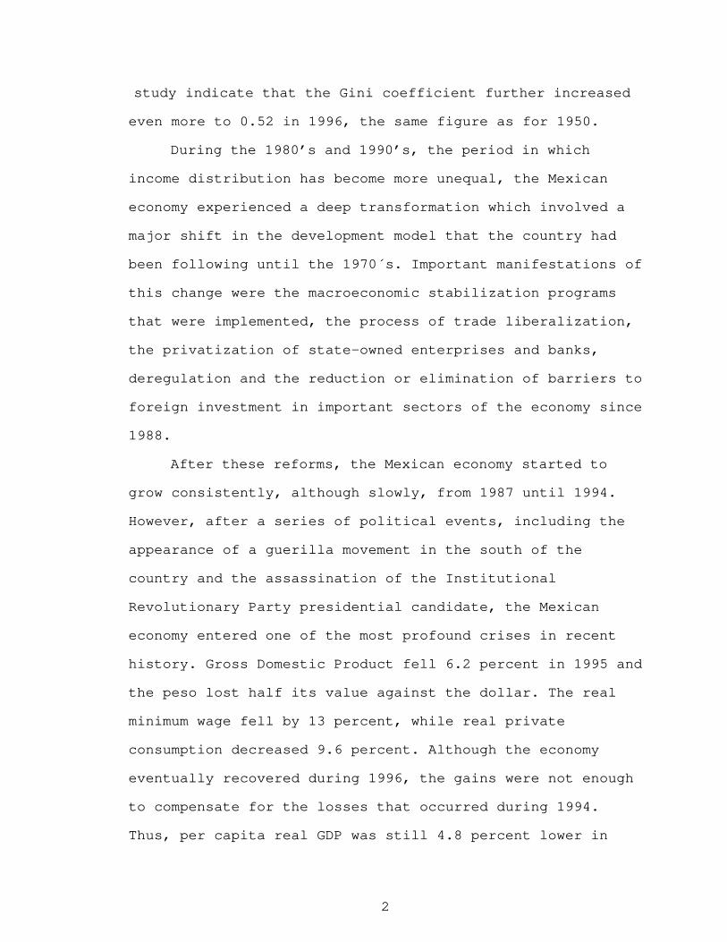
During the 1980’s and 1990’s, the period in which

income distribution has become more unequal, the Mexican

economy experienced a deep transformation which involved a

major shift in the development model that the country had

been following until the 1970´s. Important manifestations of

this change were the macroeconomic stabilization programs

that were implemented, the process of trade liberalization,

the privatization of state-owned enterprises and banks,

deregulation and the reduction or elimination of barriers to

foreign investment in important sectors of the economy since

1988.

After these reforms, the Mexican economy started to

grow consistently, although slowly, from 1987 until 1994.

However, after a series of political events, including the

appearance of a guerilla movement in the south of the

country and the assassination of the Institutional

Revolutionary Party presidential candidate, the Mexican

economy entered one of the most profound crises in recent

history. Gross Domestic Product fell 6.2 percent in 1995 and

the peso lost half its value against the dollar. The real

minimum wage fell by 13 percent, while real private

consumption decreased 9.6 percent. Although the economy

eventually recovered during 1996, the gains were not enough

to compensate for the losses that occurred during 1994.

Thus, per capita real GDP was still 4.8 percent lower in

3

1996 as compared to 1994, average real wages were 22

percent lower than in 1994 and real private consumption was

7.5 percent below the 1994 figure.

During the 1994-1996 period there was a slight

improvement in income distribution in the country. The Gini

Index decreased from 0.5338 in 1994 to 0.5191 in 1996. The

income share of the lowest three deciles increased slightly

and the share of the highest decile decreased. However, a

closer look at the income distribution reveals that the

persons situated in the lowest three percentiles of the

distribution, the poorest of the poor, reduced their share

during the period.

According to the estimates obtained by Garza-Rodríguez

(2000), both moderate and extreme poverty increased in

Mexico during the 1994-1996 period, and both the depth as

well as the severity of poverty also increased in the same

period. Although the author did not decompose the poverty

changes as due to decrease in income and the worsening of

income distribution, it is possible that both factors played

a role in the increase in poverty levels that occurred

during the period. Thus, although the Gini coefficient

declined during the period, indicating a reduction in income

inequality, the Lorenz curves for the two years intersect in

the lower percentiles of income, which indicates that the

income share of the poorest of the poor decreased during the

period.

4

The poverty profiles constructed by the author for

both years indicate that although poverty is predominantly

rural in Mexico (60 percent of the rural population was poor

in 1996), urban poverty more than doubled during the period,

from 9 percent of urban population in 1994 to 21 percent in

1996. This indicates that although poverty alleviation

programs should concentrate in the rural sector, the urban

sector should not be neglected when designing and

implementing policies to mitigate poverty.

Another variable that the poverty profiles suggested as

an important determinant of poverty was the level of

education of the household head. In both years considered in

the study, poverty incidence was higher the lower the level

of instruction of the household head. For example, 58

percent of the number of people living in households headed

by persons with no instruction was poor in 1996, while only

2.7 percent of the number of people living in households

headed by persons with at least a year of college was poor

in the same year.

Suggesting a strong correlation between poverty and

occupation of the household head, poverty incidence is

higher for households whose head works in a rural occupation

or in a domestic occupation and it is lower for households

whose head works in a professional occupation or in a middle

level occupation.

The poverty profiles also showed that poverty rates are

higher for households with the following characteristics:

5

they live in rural areas, have more than five family

members, their head has a low level of education and works

in the primary sector or in a domestic occupation.

To test the hypothesis about the determinants or

correlates of poverty we use a logistic regression with the

dependent variable being the dichotomous variable of whether

the household is extremely poor (1) or is not extremely poor

(0). The explanatory variables considered in the analysis

were: gender, age, education, the occupation of the

household head, and size and location (rural or urban) of

the household.

The study is organized as follows: Chapter II reviews

the literature about the magnitude and evolution of poverty

in Mexico during the last two decades. This chapter also

deals with the few papers that have been written about the

determinants or correlates of poverty and the methodology

they use.

Chapter III describes the ENIGH 1994 and 1996 Surveys,

and the selection of variables from the (1996) Survey that

will be used in this study.

Chapter IV presents the results of the multivariate

analysis to explore the correlates or determinants of

poverty in Mexico based on the 1996 ENIGH dataset. A

logistic regression is run, with the dependent variable

being the dichotomous variable of whether the household is

extremely poor (1) or not extremely poor (0). The

explanatory variables considered in the analysis were:

6

gender, age, education and occupation of the household

head, size and the location (rural or urban) of the

household.

Finally, Chapter V proposes some conclusions based on

the analysis developed in this study.

7

CHAPTER II

LITERATURE REVIEW

2.1 Economic Development and Poverty

It has now for some time been recognized that the

concept of economic development should not be limited to be

equivalent to economic growth alone, or even to economic

growth with an adequate distribution of income. The current

consensus recognizes that there cannot be economic

development without the reduction of poverty. Meier (1984)

notes that, as far back as 1953, Viner (1953) warned against

a limited definition of economic development, one that does

not include the reduction of massive poverty, but noted that

that notion was far away from the mainstream of economics at

that time.

Chenery (1974) brought the question of distribution

into the picture again. He noted that despite high growth in

some developing countries during the 1960´s and 1970´s, most

of the population in those countries did not benefit from

high growth, because low-income groups did not share in the

increased income.

8

Seers (1979) went beyond the problem of inequality to

include progress in reduction of poverty. He said that the

reduction of unemployment should be a requirement to be able

to say that a country is developing. In his view, un- or

under-employment is an important cause of poverty and

economic development involves reducing un- or under-

employment.

2.2 Poverty and Welfare

The World Bank (1990) defines poverty as “the inability

to attain a minimum standard of living”. Lipton and

Ravallion (1995) state that “poverty exists when one or more

persons fall short of a level of economic welfare deemed to

constitute a reasonable minimum, either in some absolute

sense or by the standards of a specific society”. Any

definition of poverty includes a given level of welfare

below which a person will be considered poor. Then, it is

necessary to determine how to assess welfare. In this

respect, there are mainly three approaches in the

literature: the welfarist approach, the basic needs approach

and the capabilities approach.

The welfarist approach bases comparisons of well-being

solely on individual utilities, which are based on social

preferences, including poverty comparisons (Ravallion,

1993). Some problems related with this approach are the need

to make inter-personal utility comparisons to obtain social

9

welfare functions, the degree of validity of full-

information and unbounded rationality assumptions on the

part of the consumers, as well as the possible conflicts

between individual maximization and valuable social

objectives (Ravallion, 1993).

The basic needs approach concentrates on the degree of

fulfillment of basic “… human needs in terms of health,

food, education, water, shelter, transport” (Streeten et.

al., 1981). The main argument behind the basic needs

approach is the possibly low correlation between income and

the degree to which these needs are satisfied.

The capabilities approach, due to Sen (1985, 1987)

considers commodities not as ends, but as means to desired

activities. Sen (1987, p.25) writes that the “value of the

living standard lies in the living, and not in the

possessing of commodities…” In this approach, poverty is

interpreted as lack of capability. The operationalization of

this approach is difficult, but an attempt has been made in

the UNDP Human Development Reports. The capabilities

approach has been criticized on the ground that it does not

clearly recognize the role individual preferences play in

welfare, thus taking the opposite extreme to the welfarist

approach.

2.3 Poverty Lines

10

The next step in poverty analysis is the definition of

one or several poverty lines, which can be absolute or

relative. This will be necessary to identify the people

living in poverty, to distinguish the poor from the non-

poor. In the absolute poverty concept, poverty is seen as a

situation of insufficient command over resources,

independent of the general welfare level in society, while

the relative poverty concept is seen as a situation of

purely relative deprivation (Hagenaars and van Praag, 1985).

Ravallion (1993, p.30) defines an absolute poverty line

as “one which is fixed in terms of living standards, and

fixed over the entire domain of the poverty comparison”,

while a “relative poverty line, by contrast, varies over

that domain, and is higher the higher the average standard

of living”.

Several approaches can be used in constructing poverty

lines, each related to a given concept of poverty. From an

absolute poverty standpoint, they can be defined using

income, total expenditure, consumption expenditure, a basket

of goods that satisfies basic needs, or food shares. From a

relative poverty standpoint, poverty lines can be defined as

a function of income or as a function of relative

deprivation in terms of commodities, that is, defining poor

households as those that are unable to attain given

commodities that are normal for their society. Hagenaars and

de Vos (1988) have proposed the use of poverty lines based

11

on subjective definitions, based on surveys asking people

whether they consider their income (or consumption) levels

to be sufficient for them. Absolute poverty definitions are

mostly used in developing countries, while relative poverty

definitions are mainly used in developed countries.

2.3.1 Basic Needs Poverty Lines

Basic needs is the most widely used approach to setting

a poverty line in developing countries. It considers the

expenditure or income necessary to obtain a given basket of

goods that satisfies basic needs, mainly food, shelter and

clothing. The first and most important component of this

estimate is food expenditure, which must be enough to

provide a minimum food-energy intake, as recommended by

nutritionists. Then some estimate of non-food expenditure is

added to this amount to obtain a total minimum expenditure.

A problem related to the estimation of the food component is

that there are many food combinations that will yield the

required minimum nutrition level and food habits vary across

regions and ethnic groups in a country. However, the most

difficult problem is estimating the non-food component of

the poverty line, since in this case there are no objective

criteria on which to base the estimate.

12

The two most widely used methods to estimate poverty

lines are the food energy method and the food-share method.

The food energy method estimates the total expenditure that

will just satisfy the recommended food-energy intake. This

is done through the use of a regression, in which the

independent variable is calorie intake and the dependent

variable can be consumption expenditures or income. This

method has the advantage that it will automatically yield

the non-food component of expenditure or income, but it has

the disadvantage that it will yield different poverty lines

across sub-groups of the population.

The food-share method estimates the cost of a food

bundle that meets the energy (calorie) and other

requirements and then divides it by the share of food in

total expenditure of a group considered to be poor. For

example, if the cost of the minimum calorie, protein, and

vitamins and other nutrients food bundle is $300, and the

share of food in the budget is 50 percent, then the poverty

line would be $600.

Another method is proposed by Lipton (1983) who argues

that the level of expenditure in which income-elasticity of

demand for food-staples is unity is where the (ultra-poor)

poverty line should be set. As Ravallion (1993) notes, the

problem with this approach is that the poverty line, thus

estimated, will shift according to all other variables

entering the demand function.

13

2.4 The Measurement of Poverty in Mexico

Although there have been relatively many studies about

income distribution in Mexico, studies about poverty have

been less frequent. The most recent studies have been

published by Hernández-Laos (1990), Levy (1994), INEGI-CEPAL

(1993), Lustig (1992 and 1995)and Székely (1995 and 1998).

Differences in methodology used by these authors make it

difficult to compare their results. The main differences in

the methodology they use are: different poverty lines,

different welfare variables (income or consumption),

different adjustments for inflation, whether the data were

adjusted to be compatible with national accounts or not and,

whether the sample was expanded to the total population.

With all these differences in methodology, different results

were obtained. Extreme poverty head-count estimates range

from 15.5 percent (Lustig (1992), using Levy’s extreme

poverty line) to 59.5 percent (Lustig (1992), using

Hernández-Laos extreme poverty line). Head-count poverty

estimates (including moderate and extreme poverty) range

from 47.4 percent (Lustig(1992), using CEPAL’s poverty line)

to 81.1 percent (Lustig(1992), using Levy's poverty line).

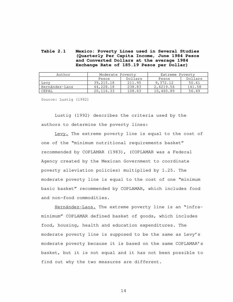
Table 2.1 shows the different poverty lines used by

each of the authors in their studies.

14

Table 2.1 Mexico: Poverty Lines used in Several Studies

(Quarterly Per Capita Income, June 1984 Pesos and Converted Dollars at the average 1984 Exchange Rate of 185.19 Pesos per Dollar)

Author Moderate Poverty Extreme Poverty

Pesos Dollars Pesos Dollars Levy 39,215.18 211.95 9,372.12 50.61 Hernández-Laos 44,228.18 238.83 2,6219.56 141.58 CEPAL 20,116.33 108.63 10,460.89 56.49

Source: Lustig (1992)

Lustig (1992) describes the criteria used by the

authors to determine the poverty lines:

Levy. The extreme poverty line is equal to the cost of

one of the “minimum nutritional requirements basket”

recommended by COPLAMAR (1983), (COPLAMAR was a Federal

Agency created by the Mexican Government to coordinate

poverty alleviation policies) multiplied by 1.25. The

moderate poverty line is equal to the cost of one “minimum

basic basket” recommended by COPLAMAR, which includes food

and non-food commodities.

Hernández-Laos. The extreme poverty line is an “infra-

minimum” COPLAMAR defined basket of goods, which includes

food, housing, health and education expenditures. The

moderate poverty line is supposed to be the same as Levy’s

moderate poverty because it is based on the same COPLAMAR’s

basket, but it is not equal and it has not been possible to

find out why the two measures are different.

15

CEPAL. The extreme poverty line includes only the

expenditure in a food basket that meets the minimum

nutritional requirements. The moderate poverty line is equal

to twice the extreme poverty line for urban areas and equal

to 1.75 times the extreme poverty line for rural areas (same

criteria than used in the INEGI/CEPAL study).

Besides the different poverty lines used by the

authors, other differences in methodology existed. Levy does

not expand the sample, while Lustig, Hernández-Laos and

CEPAL expand it. Hernández-Laos and CEPAL adjust the data to

be consistent with national accounts, while Levy and Lustig

do not. Also, Hernández-Laos does not correct the data for

inflation, which at the time the survey was done was

significant; Levy and Lustig adjust the data for inflation

while it is not clear whether CEPAL adjusts it or not.

The Mexican National Institute of Statistics, Geography

and Informatics (INEGI) and the Economic Commission for

Latin America (CEPAL) carried out another study in December

of 1993. The study, “Magnitude and Evolution of Poverty in

Mexico 1984-1992” was based on the National Survey of

Household Incomes and Expenditures (ENIGH) for 1984, 1989

and 1992. INEGI/CEPAL considered two poverty lines, one for

extreme poverty and the other called “intermediate poverty”.

The first concept included all households that did not

have sufficient income to buy a minimum food basket that met

indispensable nutritional requirements as estimated by

CEPAL. The “intermediate” poverty line is equal to twice the

16

extreme poverty line (twice the minimum food basket

expenditure) for urban areas and 1.75 times the extreme

poverty line for rural areas.

It is generally accepted that a poverty line which

covers only minimum food expenditures can be considered an

ultra-poverty line, while if that ultra-poverty line is

multiplied by the reciprocal of the food share expenditure

of the poor we obtain a poverty line that considers minimum

food expenditure plus non-food expenditures. Based on this

reasoning, it could be said that what INEGI/CEPAL calls

“intermediate” households are in fact households living in

what might be called “moderate” poverty. The income of these

households is more that enough to buy the minimum food

consumption basket, but it is less than enough to buy both

this food basket and the non-food consumption basket.

With these definitions in mind, we can analyze the

estimates made by INEGI/CEPAL. For the 1992 ENIGH survey,

they found that 13.6 million people, 16 percent of the

population, were living in extreme poverty and 23.6 million

people, or 28 percent of the population were considered

“intermediate” households, or what might be considered

“moderate” poverty as mentioned above. Adding both figures,

we could obtain an estimate of poverty in Mexico for 1992,

an estimate that includes people living in extreme poverty

and people living in moderate poverty. According to these

figures, 37.2 million people, representing 44 percent of the

population were in poverty in that year.

17

These are national figures, including both rural and

urban areas. Poverty in rural areas was much higher, 26

percent of the rural population were extremely poor and 29

percent moderately poor, meaning that more than half of

Mexico’s rural population (55 percent) was poor in 1992.

Although at first sight these figures seem exaggerated, as

defined by the study itself, they include only the income

needed to buy a minimum food consumption basket that meets

minimum nutrition requirements (extreme poverty line) and

the income needed to buy this food basket plus a minimum

non-food basket ("intermediate” or moderate poverty).

Other more recent studies of poverty include the PhD

dissertations by Alarcón (1993) and Castro-Leal (1995).

Alarcón uses Levy´s methodology to calculate HC, FGT and PG

for 1989 and compares them with Levy´s results for 1984. She

found that all three poverty measures increased in the

period considered. Extreme poverty increased from 20 percent

of the population in 1984 to 24 percent in 1989. Rural areas

registered the largest increase in poverty, increasing from

37 percent of the population in 1984 to 42 percent in 1989,

while poverty in urban areas increased from 10 percent of

the population in 1984 to 12 percent in 1989.

The poverty gap increased from 0.06 in 1984 to 0.08 in

1989, with again the rural areas experiencing the largest

increase, rising from 0.12 to 0.16. The FGT2 index, which

measures the severity of poverty, increased from 0.026 in

1984 to 0.039 for the national measure and from 0.057 in

18

1984 to 0.080 in 1989 for rural areas. Since Alarcón uses

COPLAMAR´s moderate poverty line criteria, the estimates for

moderate poverty that she obtains are very large and

controversial. They are based on the pattern of consumption

of the seventh income decile of the Mexican population.

Measured by the Headcount Index, Alarcón found a slight

decrease in total poverty, from 81 percent of the population

in 1984 to 79 percent in 1989. However, the poverty gap and

the FGT index increased slightly. PG increased from 0.46 in

1984 to 0.47 in 1989, while FGT increased from 0.30 to 0.32

in the same period.

In her PhD dissertation, Castro arrives at different

conclusions about changes in poverty incidence between 1984

and 1989, but she uses a different methodology than Levy and

Alarcón. Castro finds that extreme poverty decreased from 14

percent of the population in 1984 to 11 percent in 1989,

while moderate poverty decreased from 66 percent of the

population in 1984 to 62 percent in 1989.

In order to take into account the composition of the

household, Castro also calculates the poverty measures using

adult equivalence scales and finds a statistically

significant decline in moderate poverty between 1984 and

1989, in contrast with the decline in extreme poverty, which

is non-significant.

19

2.5 Studies about the Determinants of Poverty

Although the construction of poverty profiles is useful

because it allows us to know whether poverty is increasing

or decreasing as well as the changes in the composition of

the population in poverty, poverty profiles do not throw

much light about the causes of poverty. They only provide a

description of poverty according to several economic,

demographic or social characteristics, but do not go in

depth as to look for the underlying causes of differences in

poverty rates across population groups and/or across time.

However, while the literature on poverty measurement is

by now relatively developed and abundant, there are very few

studies dealing with finding the determinants or causes of

poverty. In general, these studies have used different

methodologies, including ordinary least square regression

where the dependent variable is continuous, logistic

regression where the dependent variable is binary, and

quantile regressions where the dependent variable is income.

In one of the first studies about the determinants of

poverty, Kyereme and Thorbecke (1991) estimated a cross-

section regression model for Ghana, using the 1974-1975

Ghana Household Budget Survey. In their model, the dependent

variable was the total calorie gap for each household in the

Survey and the explanatory variables were a set of economic,

demographic and geographic location variables. They found

that income and education of the household are inversely

20

related to household calorie gap.

Rodríguez and Smith (1994) used a logistic regression

model to estimate the effects of different economic and

demographic variables on the probability of a household

being in poverty in Costa Rica. The data they used was from

a national household-income survey carried out in 1986.

Among other results, the authors found that the probability

of being in poverty is higher the lower the level of

education and the higher the child dependency ratio, as well

as for families living in rural areas.

Coulombe and McKay (1996) used multivariate analysis to

analyze the determinants of poverty in Mauritania based on

household survey data for 1990. They estimated a multinomial

logit model for the probability of being in poverty

depending on household-specific economic and demographic

explanatory variables. The authors found that low education,

living in a rural area and a high burden of dependence

significantly increase the probability of a household being

poor.

2.6 Studies about the Determinants of Poverty in Mexico

Studies about the determinants of poverty in Mexico are

few, and they use different methodological approaches.

Cortés (1997), using the ENIGH 1992, estimates a

logistic regression of the probability of being poor as a

21

function of several economic, demographic and location

variables. He finds that the probability of being poor

decreases with the number of years of education and

increases with the burden of dependency and if the household

is located in a rural area.

Székely (1998), using a different approach and based on

the 1984, 1989 and 1992 Surveys reaches the conclusion that

lack of education is the single most important factor in

explaining poverty in the country. Other variables that he

found as directly related to poverty are: household size,

living in a rural area, and occupational disparities.

22

CHAPTER III

THE DATA

3.1 Overview

This thesis uses the information contained in the micro

data from the National Surveys of Incomes and Expenditures

of Households (ENIGH) for 1994 and 1996, carried out in

those years by the Instituto Nacional de Estadistica,

Geografia e Informatica (INEGI), Mexico´s national institute

of statistics. Although the most recent survey that has been

carried out was for 1998, the micro data for this survey has

not yet been made available to the public, so that the 1994

and 1996 surveys are the most recent surveys that have been

published by INEGI. These surveys are directly comparable

since they follow the same methodology, using the same

conceptual framework, reference period, and sample design.

The 1994 survey has 12,815 observations while the 1996

survey has 14,042 observations. Each survey was carried out

during the third quarter of the year.

23

3.2 Survey Methodology

The surveys’ sampling unit is the house and the unit of

analysis is the household. The household and its members can

be classified according to various socio-economic and

demographic characteristics such as income and occupational

characteristics, the physical characteristics of the

residence and the services available to the residents of the

household.

3.2.1 Socio-demographic Characteristics

The characteristics included in the Survey are the

following (and refer to the household residents): kinship

relationship with the household head, gender, age,

instruction level attained, school attendance, literacy

status, and type of school attended.

3.2.2 Occupational Characteristics of Household Members.

The Survey’s questionnaire asks about the labor force

activity of household members, i.e. if they belong to the

economically active population or to the economically

inactive population. The economically active population

includes the employed population and the unemployed

population actively seeking employment. The employed

population comprises the population 12 years and older who

24

declared that they worked at least one hour a week. The

unemployed population included those 12 years and older who

were unemployed and actively looking for a job at the time

of the interview. The economically inactive population

includes housewives, students, retirees, renters,

permanently disabled workers and discouraged workers who are

no longer seeking work because they have been unable to find

a job.

3.2.3 Economic Transactions.

The economic transactions considered in the surveys are

current transactions and financial or capital transactions.

Current transactions are defined as those whose object is to

cover basic needs and the result is not cumulative.

Financial or capital transactions are those motivated by the

desire to accumulate.

Current transactions include current income and current

expenditures. Current income includes both monetary and non-

monetary income (in-kind payments) received by household

members during the reference period. The income concept

registered in the surveys is net income, after deducting

taxes, social security payments, union payments or other

deductions. Current monetary income includes the following

sources: wages, entrepeneurial income, rents, incomes from

cooperatives, transfer payments and other current income.

25

Non-monetary income comprises: auto-consumption (household

production consumed in the household), in-kind payments,

gifts, and the imputed rent from owner-occupied housing.

3.2.4 Survey’s Reference Periods

There were different reference periods for the

variables included in the Surveys. For the socio-demographic

variables the reference period was at the moment of the

interview. For the income variable, the reference period was

for one month before the interview up to six months before

the interview. For the occupational characteristics the

reference period was the month before the interview.

3.2.5 Survey’s Geographic Coverage

The Survey is statistically representative at the

national level and at the urban and rural level. According

to INEGI this characteristic makes it impossible to obtain

inferences at the state level, except for a few states in

which the sample was expanded to permit inferences at the

state level. These states paid for the cost of the expanded

surveys. For the 1994 Survey, the sample was expanded for

the states of Aguascalientes, Coahuila, Mexico, Puebla,

Veracruz and the Metropolitan Mexico City Area. For the 1996

Survey the sample was expanded for the states of Campeche,

Coahuila, Guanajuato, Hidalgo, Jalisco, Estado de México,

26

Oaxaca, Tabasco and the Metropolitan Mexico City Area.

However, the analysis in the following chapters is performed

only at the national level and at the rural and urban

levels, and no analysis is done for the particular states

mentioned above.

3.3 Sampling Design

The ENIGH data were obtained through a two-stage

stratified sampling design. First stage sampling units are

Areas Geoestadisticas Basicas, AGEBS (basic geo-statistic

areas) and second stage sampling units are housing units.

AGEBS in urban areas measure around 20 to 80 blocks.

The Surveys include information about expansion factors

for each selected house, and they are equal to the inverse

of the probability of selection. In this sense, the

expansion factor for each selected house indicates the

number of houses that each house represents in the total

population of dwelling units.

Although the Primary Sampling Units corresponding to

each observation are not released by INEGI in the compact

disc that contains the surveys, we were able to obtain them

directly from INEGI for the 1996 survey, but not for 1994.

Thus, it is possible to obtain statistical inferences using

the complete information from the sampling design for 1996,

but not for 1994, in which case we only used the strata

information, but not the Primary Sampling Units information.

27

3.4 Poverty Lines used in this Study

Instead of calculating a new poverty line to be used in

this study we decided to follow the majority of studies

written about poverty in Mexico by using the poverty line

estimated by COPLAMAR (1983). COPLAMAR considers two poverty

lines, one delimiting extreme poverty and the other

delimiting moderate poverty. The extreme poverty line

constructed by COPLAMAR includes only the necessary income

to buy a minimal food bundle, including 34 different items

equivalent to 2082 calories per day per adult. The moderate

poverty line includes, besides food, minimum standards for

expenditures in housing, health and education.

Using these COPLAMAR poverty lines Székely (1998)

updated the extreme and moderate poverty lines for 1992,

equal to 92,986 pesos per head per month and 167,949 pesos

per head per month, respectively. We took these poverty

lines calculated by Székely (1998) and inflated them using

the CPI for families with incomes below a minimum wage (for

the extreme poverty line) and for families with incomes

between one and three minimum wages (moderate poverty line).

These poverty lines are shown in Table 3.1.

Table 3.1 Poverty Lines, 1994-1996 (Current Pesos per

28

Capita per Month)

1994 1996 Extreme Poverty 109 204 Moderate Poverty 197 367

Source: Author´s calculations, based on Székely (1998)

29

CHAPTER IV

THE DETERMINANTS OR CORRELATES OF POVERTY IN MEXICO

4.1 Introduction

Garza-Rodríguez (2000) analyzed the evolution of

poverty levels and poverty profiles during the period 1994-

1996. He looked at the issue of what happened to poverty

during the period as well as what happened to the

composition of the poor according to several demographic and

socioeconomic characteristics. This knowledge can be useful

since it allows us to know whether poverty is increasing or

decreasing as well as the changes in the composition of the

poor. However, it does not provide us with much insight

about the causes of poverty. For example, is poverty higher

in rural areas only because education attainment is low and

family size is high in rural areas or is poverty high in

rural areas even if we control for those variables?

While the literature on the measurement of poverty is

relatively abundant, studies about the determinants or

causes of poverty are scarce. However, it is precisely in

this area where research can be most useful, since the main

causes of poverty need to be understood in order to be able

30

to design the most efficient policies to reduce it.

There are several approaches that can be taken in the

analysis of the causes of poverty. If we follow the income

approach, poverty can be thought as being caused by lack of

income, which in turn can be caused by reduced command of

economic resources available to the household. Thus, in

general terms, poverty can be thought as being due to the

limited amount of assets owned by the poor and to the low

productivity of these assets.

Many variables can be considered as the determinants of

income, and thus, of poverty. We can divide these variables

into two general areas: the characteristics associated with

the income generating potential of individuals and the

characteristics associated with the geographic context in

which the individual lives. The first kind of

characteristics would include, for example, the assets owned

by the individual, both physical and human, while the second

type of characteristics would include, for example, the

place in which the individual lives (urban or rural).

However, there are severe problems in determining the

direction of causality. Does poverty cause the

characteristic or is it the presence of a given

characteristic which causes poverty?. An example of this

problem is whether poverty causes large households or a

large household causes poverty. It is necessary to determine

the direction of causality, but this is a difficult task

that has not been solved yet due among other things to the

31

unavailability of better data, especially panel data in

developing countries. What we will try to do in this chapter

is to get an approximation about the determinants of

poverty, even if they could more properly be called the

correlates of poverty.

We also need to separate the effects of correlates. For

example, if we find that poverty is highly correlated with

rural location, and rural location is highly correlated with

low education, then we need to know how much poverty is due

to rural location and how much is due to low education. We

approach this problem through the use of multivariate

analysis, using a logistic regression. In order to explore

the correlates of poverty with the variables thought to be

important in explaining poverty a logistic regression model

was estimated, with the dependent variable being the

dichotomous variable of whether the household is extremely

poor (1) or not extremely poor (0). The explanatory

variables considered in the analysis were: gender, age,

education and occupation of the household head, and size and

location (rural or urban) of the household.

In this model, the response variable is binary, taking

only two values, 1 if the household is extremely poor, 0 if

not.

The probability of being extremely poor depends on a

set of variables x so that

)´F(-10)Prob(Y

)´F(1)(Y Prob

xβxβ

====

(4-1)

32

Using the logistic distribution we have:

),´Λ(

11)Prob(Y

´x

´x

xβ=+

== β

β

e

e

(4-2)

Where Λ represents the logistic cumulative

distribution function.

Then the probability model is the regression:

)'F(

)]'1[F( )]'F(-0[1]|E[y

xβxβxβx

=+=

(4-3)

4.2 Empirical Results

The estimated regression is shown in Table 4.1. Except

for gender of the household head and industrial occupation,

all of the coefficients in the regression are significantly

different from zero at the 95 percent confidence level. The

variables that are positively correlated with the

probability of being poor are: size of the household, living

in a rural area, working in a rural occupation and being a

domestic worker. The variables that are negatively

correlated with the probability of being poor are: having at

least one year of primary education, having completed

primary education, having at least a year of secondary

education, having at least a year of preparatory school

(senior high school) and having at least a year of college.

33

Besides education, other variables negatively correlated

with poverty are age of the household head, working in a

professional occupation and working in a middle level

occupation.

Table 4.1 Logistic estimates of poverty determinants

Number of observations=14042 chi2(14)=3144.28 Prob > chi2=0 Log Likelihood =-3829.7657 Pseudo R2=0.291

PINDEXT Coef. Std. Err. z P>|z| [95% Conf. Interval]

FEMALE 0.0053611 0.1061904 0.05 0.96 -0.2027683 0.2134904

RURAL 1.100304 0.0789172 13.943 0 0.9456291 1.254979

HHSIZE 0.3453314 0.0125041 27.618 0 0.3208239 0.369839

AGE -0.0348488 0.0023971 -14.538 0 -0.0395471 -0.0301505

PROFOCUP -0.7083106 0.2850134 -2.485 0.013 -1.266927 -0.1496947

RURALOCUP 0.8476774 0.1016767 8.337 0 0.6483947 1.04696

INDOCUP 0.0403985 0.1134476 0.356 0.722 -0.1819548 0.2627518

MIDDLEOCUP -0.5731112 0.1295563 -4.424 0 -0.8270368 -0.3191856

DOMESTICOC 0.4777243 0.1515968 3.151 0.002 0.1806001 0.7748486

INCELEM -0.3958658 0.0757204 -5.228 0 -0.5442751 -0.2474564

COMPELEM -0.8177559 0.0935378 -8.743 0 -1.001087 -0.6344252

ATLSOMEHS -1.347069 0.1244239 -10.826 0 -1.590935 -1.103203

ATLSOMEPREP -2.096054 0.2614024 -8.018 0 -2.608394 -1.583715

ATLSOMEUNIV -3.600028 0.5973537 -6.027 0 -4.77082 -2.429237

CONSTANT -2.4781 0.1746701 -14.187 0 -2.820447 -2.135753

The variables in Table 4.1 are defined as follows:

DEPENDENT VARIABLE:

PINDEXT Binary variable indicating whether a

household is below the extreme poverty line

34

or not (1 if extremely poor, zero if not).

INDEPENDENT VARIABLES:

FEMALE Binary variable indicating whether the

household head is female or male (1 if

female, zero if male).

RURAL Binary variable indicating whether a

household is located in a rural area (less

than 15,000) or in an urban area (1 if

located in rural area, zero if not).

HHSIZE Size of the household.

AGE Age of the household head.

PROFOCUP Binary variable indicating whether the

household head works in a professional

occupation or not.

INDOCUP Binary variable indicating whether the

household head works in an industrial

occupation or not.

MIDDLEOCUP Binary variable indicating whether the

household head works in a middle level (white

collar) occupation or not.

DOMESTICOC Binary variable indicating whether the

household head works in a domestic

occupation or not.

INCELEM Binary variable indicating whether the

35

household head has incomplete elementary

education or not.

COMPELEM Binary variable indicating whether the

household head has completed elementary

education or not.

ATLSOMEHS Binary variable indicating whether the

household head has at least a year of high

school or not.

ATLSOMEPREP Binary variable indicating whether the

household head has at least a year of senior

high school or not.

ATLSOMEUNIV Binary variable indicating whether the

household head has at least a year of college

or not.

4.2.1 Model’s Predictive Power

In order to assess the predictive power of the model, a

classification table of correct and incorrect predictions

was constructed, based on the predicted probability of being

36

poor. A probability equal or greater than 0.5 was

interpreted as a prediction of a household being extremely

poor, while a probability lower than 0.5 was interpreted as

a prediction of a household not being extremely poor. Table

4.2 shows the classification table for the model. In this

table, “D” represents the number of poor households in the

sample while “~D” represents the number of not poor cases in

the sample. The symbol “+” represents the number of

households predicted as poor by the model while “-“

represents the number of not poor cases predicted by the

model.

37

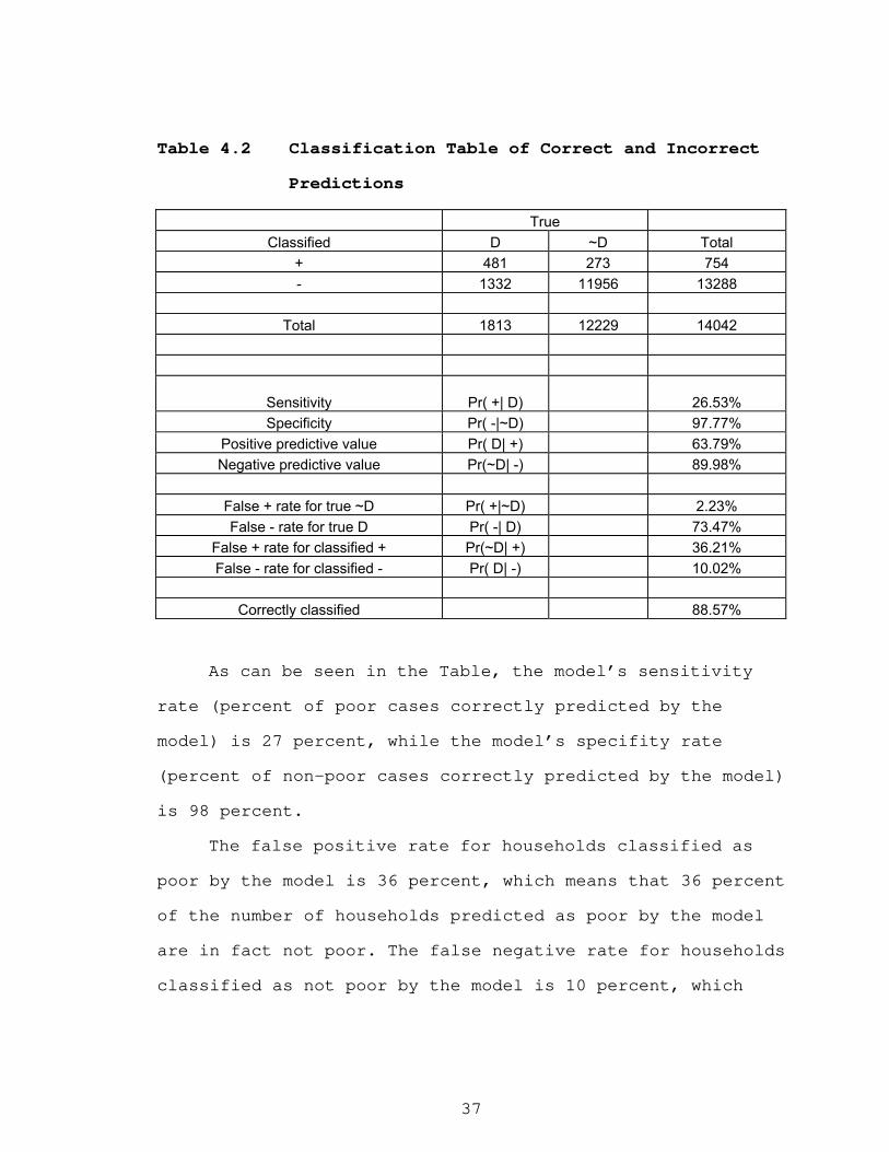
Table 4.2 Classification Table of Correct and Incorrect

Predictions

True

Classified D ~D Total

+ 481 273 754

- 1332 11956 13288

Total 1813 12229 14042

Sensitivity Pr( +| D) 26.53%

Specificity Pr( -|~D) 97.77%

Positive predictive value Pr( D| +) 63.79%

Negative predictive value Pr(~D| -) 89.98%

False + rate for true ~D Pr( +|~D) 2.23%

False - rate for true D Pr( -| D) 73.47%

False + rate for classified + Pr(~D| +) 36.21%

False - rate for classified - Pr( D| -) 10.02%

Correctly classified 88.57%

As can be seen in the Table, the model’s sensitivity

rate (percent of poor cases correctly predicted by the

model) is 27 percent, while the model’s specifity rate

(percent of non-poor cases correctly predicted by the model)

is 98 percent.

The false positive rate for households classified as

poor by the model is 36 percent, which means that 36 percent

of the number of households predicted as poor by the model

are in fact not poor. The false negative rate for households

classified as not poor by the model is 10 percent, which

38

means that 10 percent of households predicted as not poor

by the model are in fact poor.

The positive predictive value rate of the model is 64

percent, which means that 64 percent of the total number of

predicted poor households is in fact poor. Negative

predictive rate is 90 percent, meaning that 90 percent of

the total number of not poor cases predicted by the model is

in fact not poor.

As a whole, the model correctly predicts 89 percent of

cases.

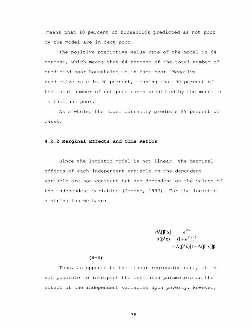
4.2.2 Marginal Effects and Odds Ratios

Since the logistic model is not linear, the marginal

effects of each independent variable on the dependent

variable are not constant but are dependent on the values of

the independent variables (Greene, 1993). For the logistic

distribution we have:

βxβ'xβ'

xβ'

xβ'

)](1)[(

)1()(

][2´x

´x

Λ−Λ=+

=Λ

β

β

e

e

d

d

(4-4)

Thus, as opposed to the linear regression case, it is

not possible to interpret the estimated parameters as the

effect of the independent variables upon poverty. However,

39

it is possible to compute the marginal effects evaluating

expression (5-4) at some interesting values of the

independent variables, such as the means of the continuous

independent variables and for some given values of the

binary variables. This is the procedure we will use in the

next sub-sections to draw graphs showing the effect of the

independent variables on poverty.

Another way to analyze the effects of the independent

variables upon the probability of being poor is by looking

at the change of the odds ratio as the independent variables

change. The odds ratio is defined as the ratio of the

probability of being poor divided by the probability of not

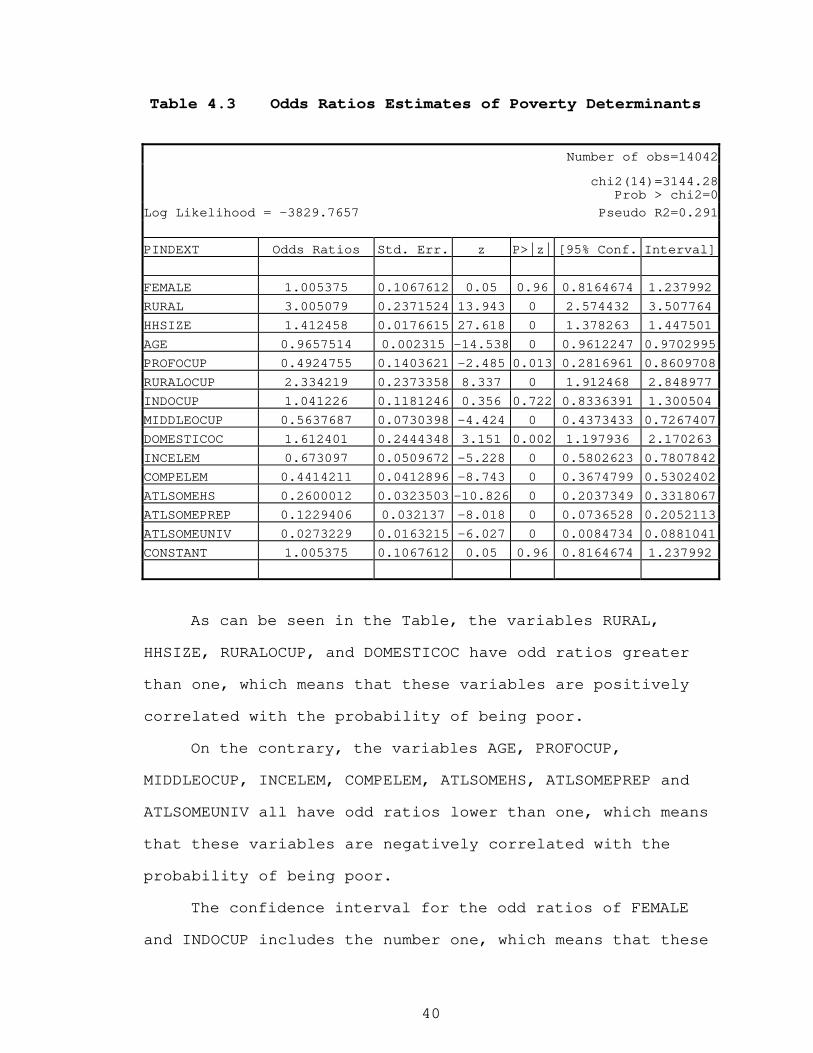
being poor. Table 4.3 shows the odd ratios for each

independent variable as well as its corresponding standard

error and confidence intervals, with the variables’ labels

being the same as in Table 4.1.

40

Table 4.3 Odds Ratios Estimates of Poverty Determinants

Number of obs=14042

chi2(14)=3144.28Prob > chi2=0

Log Likelihood = -3829.7657 Pseudo R2=0.291

PINDEXT Odds Ratios Std. Err. z P>|z| [95% Conf. Interval]

FEMALE 1.005375 0.1067612 0.05 0.96 0.8164674 1.237992

RURAL 3.005079 0.2371524 13.943 0 2.574432 3.507764

HHSIZE 1.412458 0.0176615 27.618 0 1.378263 1.447501

AGE 0.9657514 0.002315 -14.538 0 0.9612247 0.9702995

PROFOCUP 0.4924755 0.1403621 -2.485 0.013 0.2816961 0.8609708

RURALOCUP 2.334219 0.2373358 8.337 0 1.912468 2.848977

INDOCUP 1.041226 0.1181246 0.356 0.722 0.8336391 1.300504

MIDDLEOCUP 0.5637687 0.0730398 -4.424 0 0.4373433 0.7267407

DOMESTICOC 1.612401 0.2444348 3.151 0.002 1.197936 2.170263

INCELEM 0.673097 0.0509672 -5.228 0 0.5802623 0.7807842

COMPELEM 0.4414211 0.0412896 -8.743 0 0.3674799 0.5302402

ATLSOMEHS 0.2600012 0.0323503 -10.826 0 0.2037349 0.3318067

ATLSOMEPREP 0.1229406 0.032137 -8.018 0 0.0736528 0.2052113

ATLSOMEUNIV 0.0273229 0.0163215 -6.027 0 0.0084734 0.0881041

CONSTANT 1.005375 0.1067612 0.05 0.96 0.8164674 1.237992

As can be seen in the Table, the variables RURAL,

HHSIZE, RURALOCUP, and DOMESTICOC have odd ratios greater

than one, which means that these variables are positively

correlated with the probability of being poor.

On the contrary, the variables AGE, PROFOCUP,

MIDDLEOCUP, INCELEM, COMPELEM, ATLSOMEHS, ATLSOMEPREP and

ATLSOMEUNIV all have odd ratios lower than one, which means

that these variables are negatively correlated with the

probability of being poor.

The confidence interval for the odd ratios of FEMALE

and INDOCUP includes the number one, which means that these

41

variables have no statistically significant effect on the

probability of poverty.

4.2.3 Poverty and Gender

Several studies have discussed the phenomenon of the

feminization of poverty, which is said to exist if poverty

is more prevalent among female-headed households than among

male-headed households. This situation might be due to the

presence of discrimination against women in the labor

market, or it might be due to the fact that women tend to

have lower education than men and therefore they are paid

lower salaries. Using a different methodology than the one

used in this chapter, Székely (1998) found no evidence that

female-headed households are more likely to be poor than

male-headed households. Using a logistic regression and the

1992 National Survey of Income and Expenditures, Cortés

(1997) finds that the probability of being poor decreases by

six percent if the household is headed by a woman.

Looking at the results of the logistic regression

estimated above, we reach the same conclusion as Székely

(1998) since even though the sign of the coefficient for

gender of the head is negative; it is not statistically

different from zero at the 95 percent confidence level.

However, as noted by Székely (1998), these results should be

viewed with care because female-headed households could be

42

under-represented in the sample because there are cultural

reasons to believe that many of the households that declared

to be headed by males are in fact headed by women.

Figure 4.1 shows the probability of being poor for male

and for female-headed households. This graph is drawn

assuming the following values for the independent variables:

the age of the household head is 44 years (the sample mean

for this variable), the household location is in a rural

area, the household’s head did not complete elementary

education and, finally, the head works in a domestic

occupation. We can see in the Figure that the probability

curves for male and female are almost the same, which shows

that the gender of the head is not significant in explaining

poverty in Mexico.

43

Figure 4.1 Probability of being poor and gender of the head

P

rob. of B

ein

g E

xtr

em

ely

Poo

r

Household Size

Male Female

0 25

0

1

4.2.4 Poverty and Age

It is argued that poverty increases at old age as the

productivity of the individual decreases and the individual

has few savings to compensate for this loss of productivity

and income. This is more likely to be the case in developing

countries, where savings are low because of low income.

However, the relationship between age and poverty might not

be linear, as we would expect that incomes would be low at

relatively young age, increase at middle age and then

decrease again. Therefore, according to life-cycle theories

we would expect to find that poverty is relatively high at

44

young ages, decreases during middle age and then increases

again at old age.

For the case of Mexico and based on the 1984, 1989 and

1992 Surveys, Székely (1998) finds that age of the head is

not relevant in explaining poverty. However, using the 1996

survey and the methodology developed above we found that age

of the head is statistically significant in explaining

poverty, although the effect is not very strong, since as

can be seen in Table 4.2 above, an increase of one year in

the age of the head decreases the odds of being poor by only

3.4 percent.

As Figure 4.2 shows, the probability of being poor

decreases with age. This graph is drawn assuming the

following values for the independent variables: household

size is 4.58 members (the mean for this variable in the

sample), the household head is male, the household location

is in a rural area, the household’s head did not complete

elementary education and, finally, the head works in a

domestic occupation.

45

Figure 4.2 Probability of being poor and age

Pro

b. of B

ein

g E

xtr

em

ely

Poo

r

Age of Household Head15 30 45 60 75 90

0

.25

.5

.75

1

4.2.5 Poverty and Household Size

Large households tend to be associated with poverty

[World Bank (1991a,b), Lanjouw and Ravallion (1994)]. The

absence of well developed social security systems and low

savings in developing countries will tend to increase

fertility rates, especially among the poor, in order for the

parents to have some economic support from the children when

parents reach old age. It might be rational for them to

increase the number of children in order to increase the

probability that they will get support when they get old.

High infant mortality rates among the poor will tend to

provoke excess replacement births or births to insure

against high infant and child mortality, which will increase

46

household size (Schultz, 1981).

For Mexico’s case Székely (1998), using the 1984, 1989

and 1992 Surveys, found that household size is relevant in

explaining poverty, while Cortés (1997), based on the 1992

Survey, found a direct relationship between poverty and the

burden of dependency. Using the 1996 data, we obtained

similar results since, as can be seen in Table 4.2 above, an

increase of one in the size of the household increases the

odds of being poor by 41 percent.

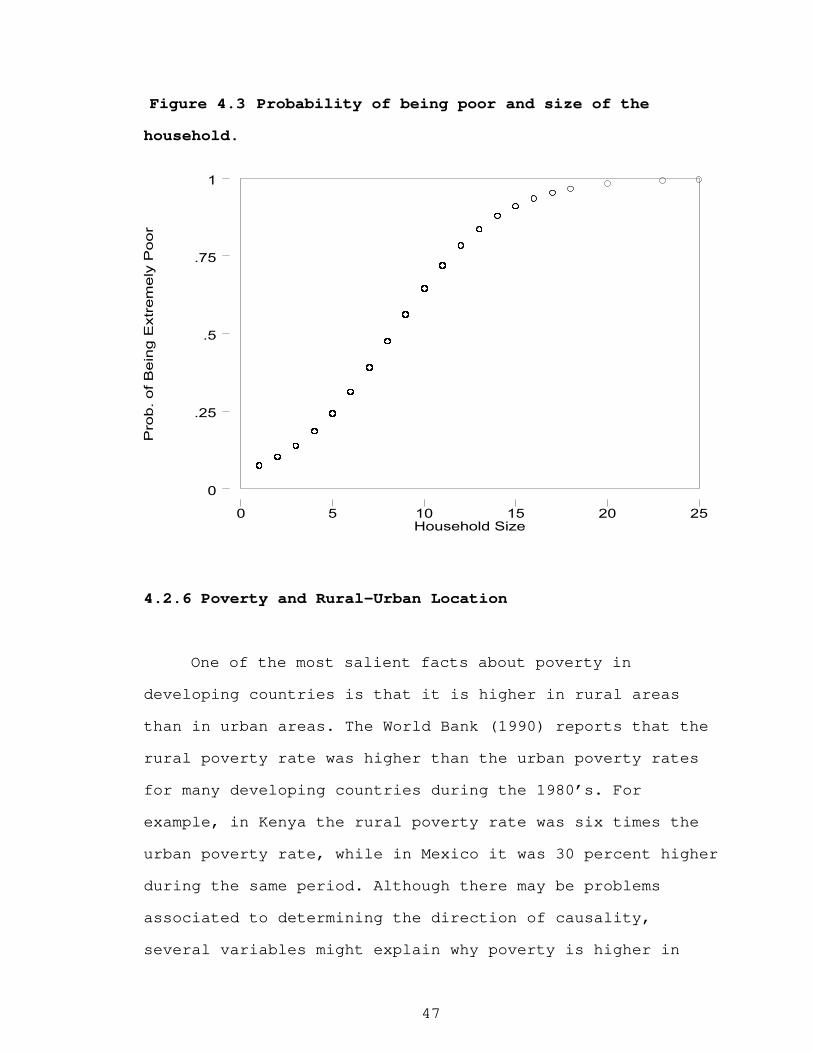
Figure 4.3 shows the probability of being poor as the

size of the household increases from its minimum to its

maximum, assuming that the independent variables take the

following values: the age of the household head is 44 years

(the sample mean for this variable), the household head is

male, household location is in a rural area, the household’s

head did not complete elementary education and, finally, the

head works in a domestic occupation.

It can be seen in Figure 4.3 that the effect of a

change in household size upon the probability of being

extremely poor is pronounced, and that this effect increases

relatively rapidly up to a household size of around 14

members and then increases less rapidly up to the maximum

household size of 25. Since 87 percent of households have

between 1 and 8 members, the first part of the curve is the

most relevant, which implies that household size has a

strong correlation with poverty in Mexico.

47

Figure 4.3 Probability of being poor and size of the

household. P

rob. of B

ein

g E

xtr

em

ely

Poo

r

Household Size0 5 10 15 20 25

0

.25

.5

.75

1

4.2.6 Poverty and Rural-Urban Location

One of the most salient facts about poverty in

developing countries is that it is higher in rural areas

than in urban areas. The World Bank (1990) reports that the

rural poverty rate was higher than the urban poverty rates

for many developing countries during the 1980’s. For

example, in Kenya the rural poverty rate was six times the

urban poverty rate, while in Mexico it was 30 percent higher

during the same period. Although there may be problems

associated to determining the direction of causality,

several variables might explain why poverty is higher in

48

rural areas than in urban areas. First, rural areas are

heavily dependent on agricultural production, which in

developing countries is characterized by low labor

productivity and therefore low incomes. Second, historically

government policy has been biased against rural areas,

including price policy, educational policy, housing, and

public services in general. Third, natural disasters such as

drought or flooding tend to affect rural areas more heavily

than they affect urban areas, and although at first we might

think that these phenomena would only affect transient

poverty they affect the stock of capital of the communities

which in turn have a permanent adverse effect on poverty

rates.

By constructing a poverty profile using the 1984

Survey, Levy (1994) concludes that poverty in Mexico is a

predominantly rural phenomenon characterized by higher

poverty rates in rural areas than urban areas. Cortés (1997)

finds that the probability of being poor increases if the

household is located in a rural area. Székely (1998) also

concludes that rural-urban location is statistically

significant as a cause of poverty in Mexico.

Our own estimates using the logistic regression for the

1996 survey indicate that rural location has a statistically

significant positive effect on the probability of being

poor. As shown in Table 4.2, the odds of being poor for a

household located in a rural area are 3 times the odds of an

urban household.

49

Figure 4.4 shows the effect of the size of the

household and rural/urban location of the household upon the

probability of being poor, assuming the following values for

the independent variables: the age of the household head is

44 years (the sample mean for this variable), the household

head is male, the household’s head did not complete

elementary education and, finally, the head works in a

domestic occupation.

It can be seen from the graph that the probability of

being poor is significantly higher for a household located

in a rural area than for one located in an urban area, and

that the difference is higher the larger the household size.

Figure 4.4 Probability of being poor and rural/urban location.

Pro

b. of B

ein

g E

xtr

em

ely

Poo

r

Household Size

Urban Rural

0 25

0

1

50

4.2.7 Poverty and Occupation

Occupation has a high correlation with poverty because

occupations which require low amounts of capital, either

human or physical, will be associated with low earnings and

therefore with higher poverty rates. In our model we found

that working in a professional occupation or in a middle

level occupation decreases the probability of being poor,

while working in a rural occupation or in a domestic

occupation increases it. Working in an industrial occupation

does not have a statistically significant effect upon the

probability of being poor.

Figure 4.5 shows the effect of the occupation variable

on the probability of poverty, based on the following

assumptions about the values of the independent variables:

household head is 44 years (the sample mean for this

variable), the household head is male, the household is

located in a rural area and the household’s head did not

complete elementary education.

It can be seen from the graph that the probability of

being poor is higher for households whose head works in a

rural occupation and in a domestic occupation and it is

lower for households whose head works in an industrial

occupation or in a professional occupation.

51

Figure 4.5 Probability of being poor and occupation

Pro

b. of B

ein

g E

xtr

em

ely

Poo

r

Household Size

Professional Rural Industrial Domestic

0 5 10 15 20 25

0

.25

.5

.75

1

4.2.8 Poverty and Education

There is generalized evidence in household surveys and

censuses that education is positively correlated with

earnings [Schultz (1988); Psacharopoulous (1985); Blaug

(1976)]. Higher earnings in turn are associated to lower

poverty levels.

Education increases the stock of human capital, which

in turn increases labor productivity and wages. Since labor

is by far the most important asset of the poor, increasing

the education of the poor will tend to reduce poverty. Thus,

we might think of low education as one of the most important

52

causes of poverty. In fact, there seems to be a vicious

circle of poverty in that low education leads to poverty and

poverty leads to low education. The poor are not able to

afford their education, even if it is publicly provided,

because of the high opportunity cost that they face. Many

times they cannot attend school because they have to work to

survive.

Both Székely (1998) and Cortés (1997) found that

education is negatively correlated with poverty in Mexico.

Székely reaches the conclusion that education is the single

most important factor in explaining poverty in the country.

The regression estimated in this chapter also finds that

education has a significant effect on the probability of

being poor.

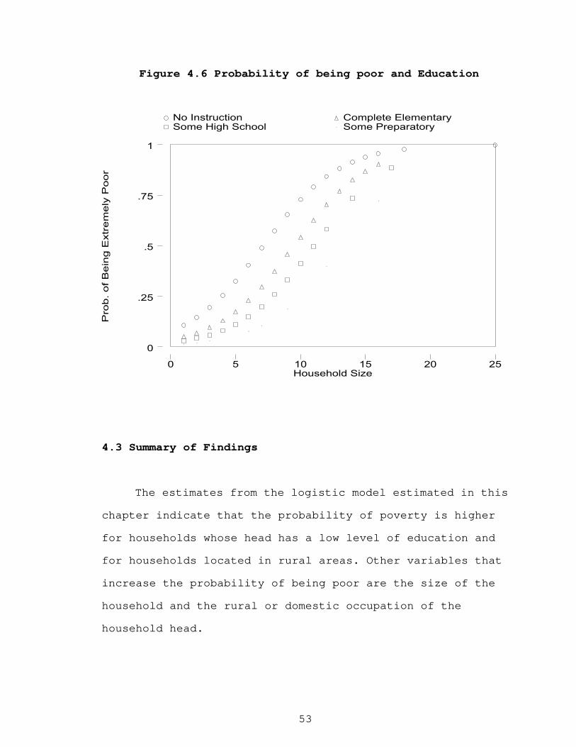
Figure 4.6 shows the effect of the level of education

on the probability of poverty, assuming that the other

independent variables take the following values: age of

household head is 44 years (the sample mean for this

variable), the household head is male, the household is

located in a rural area and finally, the head works in a

domestic occupation.

Figure 4.6 shows that the probability of being poor

decreases as the level of education increases.

53

Figure 4.6 Probability of being poor and Education

P

rob. of B

ein

g E

xtr

em

ely

Poo

r

Household Size

No Instruction Complete Elementary Some High School Some Preparatory

0 5 10 15 20 25

0

.25

.5

.75

1

4.3 Summary of Findings

The estimates from the logistic model estimated in this

chapter indicate that the probability of poverty is higher

for households whose head has a low level of education and

for households located in rural areas. Other variables that

increase the probability of being poor are the size of the

household and the rural or domestic occupation of the

household head.

54

CHAPTER V

CONCLUSIONS

Reflecting the results obtained by Garza-Rodriguez

(2000) in the construction of poverty profiles, the multi-

variate analysis developed in this study shows that the

variables that are positively correlated with the

probability of being poor are: size of the household, living

in a rural area, working in a rural occupation and being a

domestic worker. The variables that are negatively

correlated with the probability of being poor are: having at

least one year of primary education, having completed

primary education, having at least a year of secondary

education, having at least a year of preparatory school

(senior high school) and having at least a year of college.

Besides education, other variables negatively correlated

with poverty are age of the household head, working in a

professional occupation and working in a middle level

occupation. We did not find evidence in this study to

support the hypothesis of the feminization of poverty, since

the parameter estimate for this variable in the logistic

regression was not statistically different from zero.

The multi-variate analysis shows that increases in

educational attainment have an important impact on reducing

the probability that a household is poor. The five binary

55

variables for education representing increasing levels of

educational achievement show that as educational achievement

increases, the probability of being poor decreases.

The logistic model shows that a rural family has a high

probability of being poor. Even when controlling for

education, the size of the household, and the other

independent variables in the regression equation, the

rural/urban variable is statistically significant and this

variable increases the odds of a household being poor

significantly. We can only speculate what factors, in

addition to poor education and a large household, result in

rural poverty. The migration from rural to urban areas is

probably selective of the most ambitious and entrepreneurial

persons, leaving the less ambitious and less entrepreneurial

household heads in the rural areas. These household heads

are more likely to be poor.

Government policy also may contribute to rural poverty

beyond the effect of poor education by providing fewer

resources to rural residents for services such as medical

care and by policies that reduce the incentives to increase

agricultural production. Poor medical care, which includes

problems in the delivery of contraceptive supplies and

services, may contribute to the larger household size in

rural areas (Chen, et al., 1990).

Suggestions for further research include the

construction of poverty profiles at the state and regional

levels, but this task could only be possible if INEGI

56

expands the ENIGH Surveys to make them representative at

the state and regional levels. Likewise, the availability of

panel data is badly needed in order to be able to construct

better models of the determinants of poverty.

57

BIBLIOGRAPHY

Alarcón Gonzalez, D. (1993). Changes in the Distribution of Income in Mexico During the Period of Trade Liberalization. Thesis (PhD). University of California, Riverside.

Blaug, Mark.(1976) “Human Capital Theory: A Slightly

Jaundiced View”, Journal of Economic Literature, 14:3 Castro-Leal, F.T. (1995). Economic Inequality,

Poverty and Growth: Mexico, 1984-1989. Thesis (PhD). The University of Texas at Austin.

Chen et. al. (1990), “Economic Development,

Contraception and Fertility Decline in México”, The Journal of Development Studies, 26(3), April 1990, pages 408-424.

Chenery, H. et. al. (1974), Redistribution with

Growth, London. COPLAMAR (1983), Macroeconomía de las necesidades

esenciales en México: situación actual y perspectivas al año 2000, México, Siglo XXI.

Cortés, Fernando, “Determinantes de la pobreza de

los hogares. México, 1992”. Revista Mexicana de Sociología, Vol. 59, núm. 2 abril-junio 1997. pp. 131-160.

Coulombe, Harold; McKay, Andrew, “Modeling

Determinants of Poverty in Mauritania”, World Development; 24(6), June 1996, pages 1015-31.

Garza-Rodriguez, Jorge (2000), “The determinants of

poverty in México: 1996”. Ph.D. diss., University of Missouri-Columbia, 2000.

Greene, William H. (1993) Econometric Analysis. New

York: Maxwell Macmillan, 2nd Edition.1993. Hagenaars, A.J.M. and van Praag, B.M.S. (1985) “A

synthesis of poverty line definitions”, Review of Income and Wealth, 31 (2):139-154.

58

Hagenaars, A.J.M and de Vos, K. (1988) “The

Definition and Measurement of Poverty”, The Journal of Human Resources, (23):211-221.

Hernández-Laos, E. (1990). “Medicion de la

intensidad de la pobreza y la pobreza extrema en Mexico (1963-1988)”, Investigacion Economica, 191, January-March, pp. 265-298.

INEGI, Encuesta Nacional de Ingresos y Gastos de los

Hogares de 1994, Instituto Nacional de Estadística, Geografía e Informática, México, 1994.

INEGI, Encuesta Nacional de Ingresos y Gastos de los

Hogares de 1996, Instituto Nacional de Estadística, Geografía e Informática, México, 1996.

INEGI-CEPAL (1993), Magnitud y Evolución de la

Pobreza en México 1984-1992, Instituto Nacional de Estadística, Geografía e Informática, México, 1993.

Kyereme, Stephen S.; Thorbecke, Erik, “Factors

Affecting Poverty in Ghana”, Journal of Development Studies; 28(1), October 1991, pages 39-52.

Lanjouw, P. and Ravallion, M. (1994) “Poverty and

Household Size”, Policy Research Working Paper 1332, the World Bank, Washington, DC.

Levy, S. (1994 ), “La pobreza en Mexico”, in La

pobreza en Mexico, causas y politicas para combatirla, Velez, F., Editor. ITAM-FCE.

Lipton, M. (1983) Poverty, Undernutrition, and

Hunger. World Bank Staff Working Paper No. 597, Washington, DC: The World Bank.

Lipton, M. (1997) . “Editorial: Poverty – Are There

Holes in the Consensus”, World Development, 25(7):1003-1007.

59

Lipton, M. and M. Ravallion, (1995) “Poverty and Policy”, in: Behrman, Jere and T.N. Srinivasan, eds., Handbook of Development Economics, Vol.IIIB, Elsevier Science B.V.

Lustig, N. (1992). “La medicion de la pobreza en

Mexico”, El Trimestre Economico, 236, pp. 725-749. Lustig, N. (1995). “ Poverty in Mexico: The Effects

of Adjusting Survey Data for Under-reporting”, Estudios Economicos, Vol. 10, pp. 3-28.

Meier, G.M. (1984). Leading Issues in Economic

Development. New York: Oxford University Press. Psacharopoulous, George (1985) “Returns to

Education: A Further International Update and Implication”, Journal of Human Resources, 20:4, pages 583-604.

Psacharopoulous, George et al.(1996) “Returns to

Education during Economic Boom and Recession: Mexico 1984, 1989 and 1992”. Education Economics;4(3), December 1996, pages 219-30.

Ravallion, M. (1993) Poverty Comparisons. Fundamentals of Pure and Applied Economics Volume 56, Harwood Academic Press, Chur, Switzerland.

Rodriguez, Adrian G.; Smith, Stephen M. “A

Comparison of Determinants of Urban, Rural and Farm Poverty in Costa Rica”. World-Development; 22(3), March 1994, pages 381-97.

Schultz, T.P. (1981), Economics of Population

Addison-Wesley. Reading, MA. Schultz, T.P. (1988), “Education Investments and

Retuns”, in: Chenery, Hollis and T.N. Srinivasan, eds., Handbook of Development Economics, Vol. 1, North Holland.

Seers, D. (1979), “The Meaning of Development” in D.

Lehman (ed.), Development Theory.

60

Sen, A.K., (1985). Commodities and Capabilities, Amsterdam,: North Holland.

Sen, A.K. (1987). The Standard of Living, Cambridge:

Cambridge University Press. Streeten, P., Burki, S.J., ul Haq, M., Hicks, N. and

Stewart, F. (1981) First Things first: Meeting basic needs in developing countries. New York: Oxford University Press.

Székely, Miguel (1995) “Poverty in Mexico during

Adjustment“, Review of Income and Wealth; 41(3), September 1995, pages 331-48.

Székely, Miguel (1998) The Economics of Poverty,

Inequality and Wealth Accumulation in Mexico. St.Antony's Series. New York: St. Martin's Press; London: Macmillan Press; in association with St. Antony's College,1998.

Viner, J. (1953), International Trade and Economic

Development, Oxford. World Bank (1990), The World Bank Annual Report

1990, Washington DC: The World Bank. World Bank (1991a), Assistance strategies to reduce

poverty. A policy paper, Washington, D.C. World Bank (1991b), Indonesia. Strategy for a

sustained reduction in poverty. Washington, D.C. World Bank (1999), World Development Indicators,

Washington DC: The World Bank.