The Design of Ambiguous Mechanisms∗

Alfredo Di Tillio †

Bocconi University,

IGIER

Nenad Kos ‡

Bocconi University,

IGIER

Matthias Messner §

Bocconi University,

IGIER, CESifo

September 21, 2016

Abstract

This paper explores the sale of an object to an ambiguity averse buyer. We show thatthe seller can increase his profit by using an ambiguous mechanism. That is, the seller canbenefit from hiding certain features of the mechanism that he has committed to from theagent. We then characterize the profit maximizing mechanisms for the seller and charac-terize the conditions under which the seller can gain by employing an ambiguous mech-anism. Finally, we propose a class of ambiguous mechanisms that are easy to implementand perform better than the best non-ambiguous mechanism.

JEL Code: C72, D44, D82.Keywords: Optimal mechanism design, Ambiguity aversion, Incentive compatibility, In-dividual rationality.

∗We thank the editor and three anonymous referees for their insightful and constructive comments that havehelped us to greatly improve the paper. For helpful discussions and comments we also thank Simone Cerreia-Vioglio, Eddie Dekel, Georgy Egorov, Eduardo Faingold, Itzhak Gilboa, Matthew Jackson, Alessandro Lizzeri,George Mailath, Massimo Marinacci, Stephen Morris, Frank Riedel, Larry Samuelson, Martin Schneider, IlyaSegal, seminar participants at Northwestern University, Universitat Autonoma de Barcelona, Universitat PompeuFabra, Yale University, participants of UECE Lisbon 2011, Workshop on Ambiguity Bonn 2011, and Arne RydeWorkshop on Dynamic Princing: A Mechanism Design Perspective 2011. The authors would like to thank theMIUR (Prin grant 2010NE9L9Z-004) for the financial support.†Dept. of Econ. & IGIER, Bocconi University; e-mail: alfredo.ditillio@unibocconi.it‡Dept. of Econ. & IGIER, Bocconi University; e-mail: nenad.kos@unibocconi.it§Dept. of Econ.& IGIER, Bocconi University; CESifo Munich; e-mail: matthias.messner@unibocconi.it

1 Introduction

Starting with the seminal work of Ellsberg (1961), experimental economists have argued that

the standard economic model for decision making under uncertainty, namely the Expected

Utility Model (henceforth EU model), performs rather poorly in describing individuals’ be-

havior in situations where subjects have very little information regarding the decision problem

they are facing. In particular, it has been shown that the overwhelming majority of individuals

tends to shy away from alternatives for which they lack the necessary information to form a

probabilistic belief about their consequences. It is well known that this aversion against uncer-

tainty/ambiguity is incompatible with the EU model.1

This inconsistency between observed decisions and the EU model has stimulated the de-

velopment of decision theoretic models that are able to accommodate ambiguity aversion. For

two recent surveys of the literature on ambiguity aversion and its axiomatic foundations, see

Gilboa (2009) and Gilboa and Marinacci (2016). While ambiguity aversion models have been

successfully applied in many areas of economics and finance,2 they have received only limited

attention in mechanism design (see the discussion of the literature below).

We consider a screening model in which a seller is selling an object to a single ambiguity

averse buyer. For most of the paper we assume that the agent’s preferences can be described by

the maxmin expected utility model (MMEU) proposed by Gilboa and Schmeidler (1989). The

agent privately observes his willingness to pay for the good, while the principal only knows the

distribution from which it has been drawn. We introduce the concept of an ambiguous mecha-

nism, i.e. a mechanism where the principal announces a set of possible standard mechanisms

(henceforth simple mechanisms), and commits to one of them without revealing to the buyer

which one he has chosen.

We then proceed to show that a seller who faces an ambiguity averse agent can strictly

benefit from using such ambiguous mechanisms. This result has wide ranging consequences.

It implies that in any mechanism design environment with ambiguity averse agents—be it auc-

tions, bilateral trade, optimal taxation, unemployment insurance, or some other setting—the

1The sense in which ambiguity aversion is incompatible with the EU model is best explained with Ellsberg’sfamous two urn example. There are two urns, each of which contains one hundred balls. Half of the balls in Urn Aare red, the other half is blue. Also Urn B is composed of balls that are either red or blue, but the decision makerhas no information about the number of balls of each color. Now consider the following two bets. Bet RA pays onedollar if in a random draw from Urn A a red ball is extracted; bet RB pays one dollar if a random draw from Urn Byields a red ball. When faced with the choice between these two bets the overwhelming majority of subjects picksbet RA. The same they do also when the pair of bets is formulated for the color blue. Within the EU framework it isimpossible to rationalize both these decisions: for each possible belief about the composition of Urn B the decisionmaker should choose the bet on a blue ball from Urn B if and only if between the two bets on red he prefers the onereferring to Urn A.

2See for instance Epstein and Schneider (2008) and Castro and Yannelis (2012) for examples of applications ofambiguity aversion in finance and general equilibrium.

1

analysis is not without loss of generality unless ambiguous mechanisms are considered.

Through the use of an ambiguous mechanism, the principal exposes the agent to ambiguity

regarding the consequences of his report. Since the agent has MMEU preferences, he associates

with each possible report the worst possible outcome that he can obtain under all the simple

mechanisms that compose the ambiguous mechanism. Different types evaluate outcomes dif-

ferently, and hence they may associate different worst case scenarios with a given report. It is

precisely this feature that makes the use of ambiguous mechanisms attractive for the principal:

the principal can design the ambiguous mechanism in such a way that each outcome function

that it contains deters the agent from a subset of his deviation possibilities. In this way each of

the simple mechanisms that compose the ambiguous mechanism can be distorted less than the

outcome function of a simple mechanism, which has to prevent the agent from all his possible

deviations.

The arguments in the preceding paragraph presume that the agent believes that the principal

might have committed to any of the elements of the ambiguous mechanism. Put differently, it

takes for granted that the agent’s (set-valued) belief over the set of outcome functions contains

at least all degenerate distributions over this set. The assumption that the agent holds such

a ‘comprehensive’ belief is reasonable if it is compatible with the principal being indifferent

between all the elements of the ambiguous mechanism, provided that the agent acts optimally

with respect to such a belief. We therefore require that all elements of an ambiguous mechanism

generate the same expected revenue under the assumption that the agent chooses his strategy

based on a comprehensive belief. We refer to ambiguous mechanisms that satisfy this condition

as consistent. A formal definition of the consistency condition is presented in Section 3. While

from a technical point of view we treat consistency as a constraint that limits the feasible actions

available to the designer, it should be interpreted as an equilibrium condition in the interaction

between the principal and the agent.

In the remainder of the paper we characterize the profit maximizing static mechanisms in

the above described environment. First, we formulate and prove a version of the Revelation

Principle that is appropriate for our context. Doing so allows us to restrict attention to di-

rect ambiguous mechanisms. We characterize (one of) the smallest optimal direct ambiguous

mechanism(s) for the case where the set of possible types of the agent is finite.3 We show that

this mechanism is composed of at most N −1 elements, where N is the number of types. The

n-th outcome function of this ambiguous mechanism assigns the good with probability one to

all types m, n,N at a price that coincides with the reported type. Thus, every outcome function

extracts the entire surplus from N−2 types. The highest type also obtains the good with proba-

bility one. However, since his transfers are used to guarantee consistency, he typically does not

have to pay a price equal to his willingness to pay. The remaining components of the outcome

3The term ‘smallest’ refers to the number of elements of the ambiguous mechanism.

2

functions (allocations and payments of type n ≤ N − 1 under outcome function n) vary with

the details of the type distribution. More specifically, we show that these components depend

on the types’ so called adjusted virtual valuations. Independently of the details of the type

distribution, these components satisfy a monotonicity condition: the probability with which

type n obtains the good under outcome function n is smaller than or equal to the probability

with which outcome function m > n assigns the good to type m. The share of surplus that the

designer can extract from the agent increases as the type set becomes larger and the probability

of each type converges to zero. In the limiting case of a non-atomic type distribution over an

interval, the optimal ambiguous mechanism extracts the full surplus from the agent.

The effectiveness of optimal ambiguous mechanisms in extracting surplus from the buyer

comes at the cost of complexity of implementation. This complexity limits the applicability of

such mechanisms to real-life scenarios. However, the broader idea that the seller could benefit

by concealing some aspects of the mechanism from the buyers (thus making it ambiguous)

can be observed in reality. Perhaps the most prominent examples are auctions with secret

reserve prices.4 In another instance, Bergemann and Horner (2010) discuss the case of Google’s

sponsored search auctions where the algorithm to pick the winner is unknown.5

In addition, we show that ambiguous mechanisms do not need to be prohibitively com-

plex to outperform non-ambiguous mechanisms. In Section 5.1 we propose a class of basic

ambiguous mechanisms which despite being easy to implement dominate all non-ambiguous

mechanisms in terms of the expected revenue they generate. We dub these mechanisms naive

ambiguous mechanisms. Essentially, a naive ambiguous mechanism can be thought of as a

choice between a take-it-or-leave-it (TOL) offer and an ambiguous bet (an Elsberg urn) with an

unknown composition of balls of two colors. Of course the agent can also opt out. If the agent

chooses the ambiguous bet he receives the object and pays half of the TOL price (receives a

50% discount) if the ball drawn out of the urn is of the color he has chosen; otherwise he gets

and pays nothing. A max-min agent with a valuation above the TOL price optimally chooses

the TOL price, which guarantees him a strictly positive payoff. An agent with a valuation be-

tween the discounted price and the full price selects the ambiguous bet; the remaining types

opt out. The naive mechanism that is constructed on the basis of an optimal TOL price outper-

forms this optimal TOL price mechanism because a part of the types below the TOL price are

induced to buy and thus contribute to the seller’s revenue.

4Ashenfelter (1989) documents the existence of secret reserve prices at the famous auction houses as Christie’sand Sotheby’s, Hendricks, Porter, and Spady (1989) in auctions for off-shore oil, Elyakime, Laffont, Loisel, andVuong (1994) in timber auctions in France, and Bajari and Hortacsu (2003) on eBay, to name a few.

5 Auctions with ex ante uncertain auction rules are also applied in the used car market. In these auctions firstbuyers submit their bids. Upon observing the bids the auctioneer either declares a winner or he calls for a secondround of bids and so on. The rule according to which the decision about whether or not to continue is taken, isnot known to buyers (and supposedly not easily inferable from previous observations unless the bidder is extremelyexperienced). We are thankful to Larry Samuelson for pointing us to this example.

3

In the final section of the paper we discuss how the result on full surplus extraction under

ambiguity aversion relates to the findings of Matthews (1983), who shows that with risk aver-

sion growing towards infinity the seller’s rents grow towards full surplus extraction.6 We then

proceed to show that the principal may want to elicit payoff-irrelevant private information from

the agent. Since such information is easy to generate, the principal has an incentive to induce

the agent to inflate his type set by adding payoff irrelevant elements.

We provide three robustness checks. First, we show that the seller benefits from ambiguous

mechanisms even if he is ambiguity averse himself. Consistency ensures that the seller obtains

the same expected payoff from all outcome functions. Therefore, even if a third person were

to choose the outcome function the seller would not be exposed to ambiguity. What is more,

we show that even if the seller’s preferences can be described by MMEU and one does not

require consistency, the mechanisms that we derive are optimal. Second, we argue that the

central insight of the paper—that the principal can exploit the agent’s ambiguity aversion by

offering an ambiguous mechanism—does not depend on the specific model of ambiguity aver-

sion we adopt (MMEU preferences) but remains valid under alternative models of uncertainty

aversion.7 More specifically, we provide an example that shows this for the case of smooth

ambiguity aversion. The third dimension in which the core insight of the paper generalizes

is the number of agents. While we do not provide a detailed characterization of the optimal

ambiguous mechanism for the case where the agents’ type sets are finite, we describe in Ap-

pendix B the mechanism that extracts the full surplus when the agents’ types are drawn from

an atomfree distribution defined on some interval.

Related literature: A number of recent papers consider mechanism design problems with

ambiguity averse players. Examples include Bose, Ozdenoren, and Pape (2006), Turocy (2008),

Bose and Daripa (2009), Bodoh-Creed (2012), Bose and Renou (2014), Bergemann and Schlag

(2011), Auster (2015), Wolitzky et al. (2014) and Kos and Messner (2015).8 The central dif-

ference between these papers and ours is that they start from the assumption that the agents

(and/or the principal) are uncertain about the other agents’ type distribution. That is, the un-

certainty in these models refers to an exogenously given variable. The endogenous objects

(i.e. the mechanisms) are not allowed to be ambiguous.9 Instead, these papers characterize the

optimal standard (i.e. non-ambiguous) mechanism, where attention is restricted either to direct

6The implications of risk aversion for the design of an optimal mechanism are also studied by Maskin and Riley(1984).

7The details of our characterization of an optimal ambiguous mechanism do depend on the assumption ofMMEU preferences.

8Several models of beliefs and behavior in games that relax the assumption of Bayesian expected-utility max-imizing players have been proposed. See e.g. Azrieli and Teper (2011) and the references therein. Moreover,ambiguity aversion has also been applied in environments with moral hazard; see Lang and Wambach (2013).

9Bose and Renou (2014) are an exception to this observation; their work is discussed in more detail in thefollowing paragraph.

4

mechanisms or to simple forms of indirect mechanisms (e.g. standard auction formats).10

To the best of our knowledge, this is the first paper showing that it can be in the designer’s

interest to introduce uncertainty over outcome functions when agents are ambiguity averse. In

a contemporaneous and independent paper, Bose and Renou (2014) also recognize that in such

contexts the principal may want to introduce some element of uncertainty into the mechanism

that he uses. The two papers are complementary, as they study the impact of ambiguity aversion

through quite distinct channels. Unlike in this paper, in their work ambiguity is not introduced

via the outcome functions. Instead, they explore which social choice rules the designer can

implement if he engages the agents in a dynamic communication game that he mediates by

transforming messages in an ambiguous way. By injecting uncertainty in the exchange of mes-

sages between the agents, the principal can manipulate the agents’ beliefs about each other’s

type and hence their behavior. Bose and Renou (2014) remark that the precise extent to which

the agents’ beliefs can be manipulated depends on the assumed form of (full Bayesian) belief

updating. By contrast, restricting attention to strategic form mechanisms makes the question of

what is the most appropriate way to model updating by ambiguity averse individuals— an issue

still controversially discussed in the literature—altogether irrelevant in our context. Finally, the

ambiguous communication devices in Bose and Renou (2014) serve to manipulate the agents’

beliefs over the other agents’ types and hence they are ineffective in single agent environments.

Instead, as we show in this paper, (outcome) ambiguous mechanisms have leverage also in the

case of a single agent.

The paper is also related to the literature on robust mechanism design that originated with

the seminal papers by Bergemann and Morris (2005) and Chung and Ely (2007). This literature

departs from the standard Bayesian type space framework that has dominated the earlier mech-

anism design literature and studies what kind of social choice functions are implementable

irrespective of the assumed type space. Requiring such a form of robustness with respect to

the details of the type space is similar in spirit to the idea of a designer who is uncertain about

the ‘correct’ type space. Apart from the fact that the ‘uncertainty aversion’ in the case of this

literature is on the side of the designer, the crucial conceptual difference to our work lies in the

fact that the family of the relevant type spaces is not an endogenous object (like the ambiguous

mechanisms in our work) but is exogenously given.

Finally, the paper also relates to the literature on ambiguity aversion in game theory (see

for instance the papers Azrieli and Teper (2011) and Bade (2011)).

10Similar comments apply both to the literature on moral hazard with ambiguity aversion and the literature onmodels with Knightian uncertainty. For the literature on moral hazard and ambiguity aversion see for instanceKellner (2015) and Szydlowski (2012); on Knightian uncertainty in mechanism design see Lopomo, Rigotti, andShannon (2009) and Garrett (2014) and the references therein.

5

2 Motivating Example

Consider a principal selling an object to an ambiguity averse and risk neutral buyer whose pref-

erences can be represented by maxmin expected utility. The buyer’s valuation for the object,

θ, is 1 with probability 1/4, 2 with probability 1/4 and 4 with probability 1/2. The seller’s

objective is to maximize expected revenue.

The optimal standard mechanism in this setting is a take-it-or-leave-it offer at the price of

4. The corresponding direct mechanism asks the agent to report his type and awards him the

object at a price of 4 if the agent announces θ = 4. For any other report the seller keeps the

object and no transfer takes place. The expected revenue generated by this mechanism is 2. It

will prove convenient to represent the described direct mechanism in the following table form,

where (q∗, t∗) denotes the outcome function (probability with which the good is transferred and

transfer to be paid) and θ denotes the reported type.

θ 1 2 4

(q∗, t∗) (0,0) (0,0) (1,4)

Table 1: The optimal non-ambiguous direct mechanism

Suppose that instead of offering the above standard mechanism (henceforth, we will refer

to such mechanisms also as simple mechanisms) the seller proceeds as follows. Before he asks

the buyer to communicate his valuation of the good, he informs him that he has committed to

a simple (direct) mechanism. But instead of letting the buyer know which simple mechanism

he has committed to he only tells him that this simple mechanism is an element of some set of

simple mechanisms that he reveals to the buyer. By not providing the buyer with any further

information about the simple mechanism to which he has committed, the seller exposes the

buyer to ambiguity about the consequences of his messages. We therefore refer to the set of

simple mechanisms that is communicated to the buyer as an ambiguous mechanism.

For the sake of concreteness, suppose the seller offers an ambiguous mechanism that con-

tains two (direct) simple mechanisms, denoted by (q1, t1) and (q2, t2), respectively.11 Assume

that the first outcome function, (q1, t1), specifies that upon a message θ = 1 the object remains

with the seller and there are no transfers. If the agent reports θ = 2, he obtains the object at a

price of 1. Finally, in case the agent’s message is θ = 4, he obtains the object and pays 4. The

second outcome function, (q2, t2), awards the object at a price of 1 to the agent if he reports

θ = 1, does not award the object to the agent, and no transfer takes place, if the agent reports11Throughout the paper we slightly abuse terminology by identifying direct mechanisms with their outcome

functions.

6

θ = 2. If the agent reports θ = 4, he receives the object with certainty and pays 4. We denote

the ambiguous mechanism composed of these two simple mechanisms by Ω. The details of Ω

are summarized in the following table.

θ 1 2 4

(q1, t1) (0,0) (1,1) (1,4)

(q2, t2) (1,1) (0,0) (1,4)

Table 2: The ambiguous (direct) mechanism Ω

We now turn to the question of how the buyer should behave when he is offered the mech-

anism Ω. The buyer’s preferences are of the max-min expected utility type, hence whenever he

is faced with a decision problem under ambiguity, he associates with each action that he may

take the payoff that this action yields in the (action specific) worst case scenario. In the context

of our example, the buyer is exposed to ambiguity through the mechanism Ω: the consequences

of a message that he can send to the seller depend on the outcome function to which the seller

has committed, and the buyer has no explicit or even implicit information regarding the seller’s

choice.

If the buyer does consider it possible that the principal might have committed to either of

the two outcome functions in Ω, then the payoff that type θ associates with a message θ is

minq1(θ)θ − t1(θ),q2(θ)θ − t2(θ).12 We will now argue that truthful reporting is an optimal

strategy for the buyer. To see this, suppose first that the buyer’s type is θ = 4. If he reports this

truthfully he obtains the object with certainty and pays a price of 4 (both simple mechanisms

specify this outcome when θ = 4). His payoff in that case is therefore 0. If he reports type 2 he

gets the object at a price of 1 if he is facing the simple mechanism (q1, t1); the corresponding

payoff is 1×4−1 = 3. On the other hand, if he is faced with (q2, t2) he does not get the object,

and does not have to pay anything. Consequently, his payoff in that case is 0. So the worst-case

payoff both for truth-telling and for reporting type 2 is equal to 0, meaning that reporting type

2 when the true type is 4 does not represent a profitable deviation. The same reasoning can be

applied to show that type 4 cannot do better by reporting 1 instead of 4. In fact, the ‘symmetry’

in the outcomes after reporting either type 1 or 2 implies that all three types are indifferent

between these two reports. Thus, in order to complete our argument we just have to show that

neither type 1 nor type 2 can do better by reporting 4 than by telling the truth. This follows

from the fact that reporting 4 implies a payment of 4, which exceeds the valuations of both

lower types.

12Remember that we have also imposed risk neutrality.

7

Under truthful reporting, both outcome functions in Ω generate an expected revenue of 9/4:

(q1, t1) : 0×14

+ 1×14

+ 4×12

=94

(q2, t2) : 1×14

+ 0×14

+ 4×12

=94.

This expected revenue exceeds the expected revenue of 2 which is achieved by the optimal

standard mechanism (which is a take it or leave it offer at a price of 4). This shows the seller

can do strictly better by adopting an ambiguous mechanism rather than limiting himself to a

standard mechanism.

The above analysis relies on two crucial assumptions on which we want to comment further.

First, in order for the ambiguous mechanism Ω to generate a higher expected revenue than the

best simple mechanism it is crucial that the seller has the possibility to commit to one of the

two simple mechanisms in Ω before the agent makes his choice. It is straightforward to see

that if the principal does not have the possibility to commit but makes his choice between

(q1, t1) and (q2, t2) ex post, then truth-telling is no longer optimal. Without commitment the

principal would always choose the first outcome function after receiving message θ = 2 and the

second one upon getting message θ = 1. But if that is the case, then type 4 of the buyer would

never want to report his type truthfully since by choosing either of the other two messages

he could get the object with the same probability but at a lower price. Thus, in the absence

of commitment to a specific outcome function in Ω, the agent can predict the seller’s ex post

choice and will thus not perceive his situation as ambiguous. But then adopting an ambiguous

mechanism cannot help the seller to achieve a higher payoff if he is not able to commit to a

specific element of the ambiguous mechanism ex ante.

Given this observation, it is important to understand that the commitment that ambiguous

mechanisms require is no stronger than the kind of commitment imposed in most of the mech-

anism design literature. The only difference is that we assume that the principal can commit

to something that the agent cannot observe before he makes his choice. We can assume that

the simple mechanism to which the principal commits is described in some document that is

stored in a place the access to which is jointly controlled by the principal and the agent (so that

ex post they can verify together which allocation-transfer pair should be implemented). Put

differently, what matters is the verifiability of the mechanism and of the messages vis-a-vis a

third party who can guarantee the correct implementation of the mechanism.

The second important assumption on which the analysis of the above example builds is the

assumption that the buyer considers it possible that the seller has committed to either of the two

outcome functions in Ω. This is a reasonable assumption in light of the fact that the seller is not

providing the buyer with any explicit information as to which outcome function he might have

chosen. However, the buyer should only really expect the seller to choose a simple mechanism

8

in Ω that yields the seller the highest profit. The possibility to indirectly infer the simple

mechanism chosen by the principal is incompatible with the idea that the buyer perceives the

mechanism that he is presented as ambiguous. We therefore impose the requirement that the

principal can offer only ambiguous mechanisms such that all their elements generate the same

expected revenue provided the agent acts optimally based on the belief that the principal might

have committed to any of the outcome functions in the ambiguous mechanism. We refer to this

condition as consistency. It is due to this consideration that we have chosen Ω in such a way

that both its simple mechanisms generate the same expected revenue.

Finally, the consistency of the proposed ambiguous mechanism guarantees that the seller

obtains the same expected revenue regardless of which of the two outcome functions is chosen.

Therefore even if the seller was ambiguity averse and a third party were to choose an outcome

function, he would not be exposed to ambiguity by the ambiguous mechanism. That is, even if

the seller is ambiguity averse himself the proposed mechanism guarantees him a higher payoff

than the best non-ambiguous mechanism.

3 Framework

Throughout the first part of the paper we consider the mechanism design problem of a principal

selling a single unit of a good to a single agent. The notation and terminology that we introduce

below generalize in the obvious way to the case of multiple agents, which we consider in

Appendix B.

Allocations and preferences. An allocation is a pair (x, τ) ∈ X ×R, where x ∈ X = [0,1]

denotes the probability with which the good is transferred to the agent, and τ the monetary

transfer the agent has to pay to the principal.13 With a slight abuse of terminology we will

typically use the term ‘allocation’ to indicate the non-monetary component x of a pair (x, τ).

The agent’s preferences over X×R depend on his type θ ∈Θ ⊂R. More specifically, we assume

that they are represented by the linear utility function

u(x, τ) = xθ−τ.

The agent’s valuation of the good, that is, his type θ, is his private information. Throughout the

first part of the paper we assume that Θ is a finite set with N elements and we index types so

that θn is increasing in n. The principal’s beliefs regarding the agent’s type are described by the

probability distribution p = (p1, . . . , pN).

13Instead of interpreting x as the probability with which the indivisible good is transferred one can equivalentlyassume that the good is perfectly divisible and that x represents the share given to the agent.

9

The agent is ambiguity averse in the sense of Gilboa and Schmeidler (1989). That is, in

a situation where his beliefs are described by a family of distributions over allocation-transfer

pairs, Λ, his utility is given by

infλ∈ΛEλ[xθ−τ].

The principal is risk and ambiguity neutral. His objective is to maximize expected revenue,

that is, the expected transfer paid by the agent. We show in Section 6.2 that our main results

go through also under the assumption of an ambiguity averse principal. Allowing for this

possibility, however, does not add anything of interest to our analysis as the central insights

that we obtain are driven by the agent’s ambiguity aversion.

Simple vs. ambiguous mechanisms. A simple mechanism is a triple (S ,q, t), where S is a

set of messages that the agent may send to the principal, and the functions q and t map S into

X and R, respectively. q(s) is the probability with which the good is transferred to the agent

if he sends message s, while t(s) is the corresponding transfer that the agent has to pay to the

principal.14 We refer to q and t, respectively, as allocation and transfer rules on S ; the pair (q, t)

is the outcome function of the mechanism. A direct simple mechanism is a simple mechanism

such that S = Θ. Since all direct mechanisms share the same message space, we drop the latter

from the notation and identify the direct mechanism (Θ,q, t) with its outcome function (q, t).

Mechanism design models typically assume that besides committing to a particular out-

come function the principal also fully and credibly reveals it to the agent. In effect, if the agent

has standard expected utility preferences then the latter part of this assumption is innocuous,

as the principal cannot gain anything from concealing this information.15 The central insight

of this paper is that this is no longer true with an ambiguity averse agent. Indeed, we show that

it is typically in the principal’s best interest not to inform the agent about the exact outcome

function he commits to. Instead, he can benefit from communicating the rules of the mecha-

nisms in an ambiguous way, by only announcing that it belongs to a certain set. The notion of

an ambiguous mechanism captures the idea of such ambiguous rules.

Definition 1 (Ambiguous mechanism). An ambiguous mechanism is a pair (S ,Ω), where S

is a set of messages, and Ω is a set of outcome functions defined on S , i.e. Ω ⊂ XS ×RS .16 A

14Note that our definition of a simple mechanism allows for random allocations but not for random transfers:the range of t is R, not the set of probability measures over R. Given that both the principal and the agent arerisk neutral, restricting attention to deterministic transfer schemes is without loss of generality. A mechanism withrandom transfers can be replaced by one with deterministic transfers that specifies for each type report the expectedvalues of the random transfer scheme. Doing so does not alter the two players’ expected payoffs for any decisionthat the agent may take. The same is true for random allocation rules if the good is perfectly divisible. If the goodis not divisible, then allowing for random allocations expands the set of possible allocations.

15Under any standard equilibrium concept the agent would know in equilibrium which function has been chosenby the principal.

16As argued earlier, the restriction to ambiguous mechanisms with (sets of) deterministic outcome functions is

10

generic element of Ω is denoted by (q, t), where q ∈ XS and t ∈ RS .

Before we go on, a few remarks on the interpretation and purpose of the concept of an

ambiguous mechanism are in order. After choosing a set of possible messages, S , the principal

commits to an outcome function (q, t). This commitment may be achieved, say, by depositing

(q, t) with an uninterested third party. The agent is not fully informed about the chosen outcome

function. Instead the principal limits himself to telling the agent that it belongs to a set Ω. Of

course, by announcing such ambiguous rules he exposes the agent to uncertainty about the

consequences of his messages, and we discuss the principal’s motives for doing so in the next

section.

The requirement that (q, t) ∈ Ω rules out the possibility that the principal completely de-

ceives the agent with regard to (q, t). We stress once more the fact that the principal commits

to (q, t) before the agent sends his message; therefore the choice of (q, t) cannot be conditioned

on the message.

Agent’s strategies and beliefs. Once the designer has specified an ambiguous mechanism,

(S ,Ω), the agent chooses a message from S . A strategy for the agent is a function σ that maps

Θ into S , i.e. σ ∈ S Θ.

We assume that the agent cannot use mixed strategies. This assumption, which is com-

monly adopted in the ambiguity literature, has some bite, as an ambiguity averse individual

facing two alternatives with uncertain consequences may strictly prefer mixing over the al-

ternatives to each of the two.17 However, we maintain that besides being pervasive in the

literature, the assumption is especially weak in our context. Unlike an expected utility max-

imizer, an ambiguity averter may ex ante wish to randomize even over alternatives that he is

not indifferent over. But if the individual has strict preferences over the alternatives he is ran-

domizing over, then the strong ex ante incentives to mix conflicts with the individual’s ex post

incentives to implement the outcome of the randomization. In this case, allowing for mixed

strategies may therefore matter only if the agent can commit to obeying the recommendation

of some randomizing device. Making such a commitment in a mechanism design context is

difficult, because the designer can do better by declining reports generated by such devices,

that is, by requiring reports to be made directly by the agent.18

without loss of generality in an environment with risk neutral players.17Ever since Raiffa (1961), it is well known that randomization may help the agent to hedge against the uncer-

tainty involved in the two alternatives. Recently Saito (2015) provided an axiomatization of ambiguity aversionwhich does not give rise to a hedging motive.

18While this argument only refers to randomizations over alternatives that the individual does not consider asequivalent, it is sufficient for our purpose. In our context, the agent will have to decide which type to report to theprincipal. The optimal direct mechanism that we will derive can be arbitrarily closely approximated by a mechanismwith the property that no type of the agent is indifferent between any two messages.

11

The set of optimal strategies for the agent depends on his beliefs regarding the outcome

function (q, t) to which the principal has committed himself. The agent’s only piece of hard

information in this respect is that the function belongs to Ω. On the other hand, the agent

knows that the principal seeks to maximize his revenue. Given the agent’s ambiguity aversion,

it thus seems appropriate to assume that his belief set contains the entire family ∆(Ω) of prob-

ability measures on Ω, provided that such a belief set is not incompatible with the principal’s

optimizing behavior in a sense that we formalize next.

For any ambiguous mechanism (S ,Ω), let Σ∗(S ,Ω) designate the corresponding set of opti-

mal strategies for the agent, when his beliefs are given by ∆(Ω). Since the agent is risk neutral,

calculating the infimum of his expected payoffs with respect to ∆(Ω) delivers the same value as

the one obtained when attention is restricted to Ω. Thus, the set Σ∗(S ,Ω) is the set of all σ ∈ S Θ

such that for each θ ∈ Θ,

σ(θ) ∈ argmaxs∈S

inf(q,t)∈Ω

[q(s)θ− t(s)].

Definition 2 (Consistency). An ambiguous mechanism (S ,Ω) is consistent with respect to σ ∈

Σ∗(S ,Ω) if under σ all outcome functions in Ω yield the same expected revenue to the principal,

i.e. if for all (q, t), (q′, t′) ∈Ω

Ep[t(σ(θ))] =Ep[t′(σ(θ))].

The ambiguous mechanism (S ,Ω) is consistent if it is consistent with respect to some σ ∈

Σ∗(S ,Ω).

Consistency requires that each element of the ambiguous mechanism Ω delivers the same

expected revenue to the principal if the agent bases his choice on the belief set ∆(Ω). To

shed further light on this condition, consider a situation were it is not satisfied. Thus, suppose

that the principal proposes an ambiguous mechanism (S ,Ω) such that for every σ ∈ Σ∗(S ,Ω)

there exist (q, t), (q′, t′) ∈Ω withEp[t(σ(θ))] <Ep[t′(σ(θ))]. In this case the agent’s assumption

that the principal might have chosen any of the elements in Ω leads to the conclusion that

the principal strictly prefers some elements of Ω over other elements of Ω, if he correctly

predicts the agent’s belief and strategy. Consistency rules out such contradictory beliefs. It

is essentially an equilibrium condition for the two stage game played by the two parties. In

equilibrium the agent should not entertain the possibility that a certain outcome function is

chosen, if the strategy that he intends to implement in response to this belief implies that the

outcome function does not maximize the designer’s payoff.19

19 In Section 6.2 we show that the assumption of consistency is without loss of generality when also the sellerhas maxmin expected utility preferences.

12

Finally, we remark that requiring the seller to be indifferent before the buyer reports his

type rather than after, is to the seller’s benefit. If the seller could choose his preferred simple

mechanism in the ambiguous mechanism after the report, he would choose a mechanism with

the highest transfer given the report. The buyer would foresee this and calculate his payoffs

accordingly. In particular, every type of the agent would associate with any given report the

same worst case scenario, namely the outcome function in Ω with the smallest probability of

trade (for that report) among the simple mechanisms that specify the highest transfer (for that

report). But then the agent’s behavior vis-a-vis the ambiguous mechanism Ω would be exactly

the same as the agent’s behavior vis-a-vis a simple mechanism that specifies only these worst

case allocations and transfers.20 Consequently, the expected revenue of the designer would

also be exactly the same. Thus, if the designer does not commit ex ante to an element in Ω, he

cannot do any better than by using only simple mechanisms.

4 Optimal ambiguous mechanisms

In designing the optimal ambiguous mechanism, the principal has to take into account two

types of constraints. First, he must respect the consistency condition that we have discussed in

the preceding section. Second, since we assume that the buyer’s participation in the mechanism

is voluntary, the principal must make sure that the mechanism allows each type of the agent to

earn at least his outside option. We assume that the latter is equal to zero for every type. Thus,

the principal’s problem is to choose among all ambiguous mechanisms (S ,Ω) for which there

exists some σ ∈ Σ∗(S ,Ω) satisfying the conditions

Ep[t(σ(θ))] =Ep[t′(σ(θ))] for all (q, t), (q′, t′) ∈Ω, (1)

inf(q,t)∈Ω

q(σ(θ))θ− t(σ(θ)) ≥ 0 for all θ ∈ Θ, (2)

the one that delivers the highest expected revenue.

In what follows we show that the principal’s problem can be substantially simplified.

4.1 The Revelation Principle

First we prove a version of the Revelation Principle that applies to our environment, by showing

that the principal can without loss of generality offer the agent an ambiguous mechanism that

(i) asks the agent to report his type, and (ii) is constructed in such a way that the agent is willing

to do so in a truthful manner.20Formally, this simple mechanism specifies the same messages, S , and its outcome function (q, t) is such that

for all s, t(s) = sup(q′,t′)∈Ωτ ∈ R : t′(s) = τ and q(s) = inf(q′,t′)∈Ωx ∈ X : q′(s) = x and t′(s) = t(s).

13

Definition 3 (Incentive compatibility). An ambiguous mechanism (S ,Ω) is direct if S = Θ,

in which case we identify the mechanism with its set of outcome functions Ω, and for all

(q, t) ∈Ω and 1 ≤ n ≤ N we write qn and tn for q(θn) and t(θn), respectively. A direct ambiguous

mechanism Ω is downward incentive compatible if

inf(q,t)∈Ω

qnθn− tn ≥ inf(q,t)∈Ω

qmθn− tm for all 1 ≤ m < n ≤ N, (DIC)

upward incentive compatible if

inf(q,t)∈Ω

qnθn− tn ≥ inf(q,t)∈Ω

qmθn− tm for all 1 ≤ n < m ≤ N (UIC)

and incentive compatible if it is both downward and upward incentive compatible.

Proposition 1 (Revelation Principle). Let (S ,Ω) be an ambiguous mechanism that is consistent

with respect to σ ∈ Σ∗(S ,Ω). The direct ambiguous mechanism

Ω′ =(q′, t′) ∈ XΘ×RΘ : q′ = qσ, t′ = t σ for some (q, t) ∈Ω

is incentive compatible and consistent with respect to truth-telling.

Proof. Proofs of the results can be found in the Appendix, unless stated otherwise.

The Revelation Principle guarantees that given any consistent ambiguous mechanism, (S ,Ω),

we can find a direct ambiguous mechanism, Ω′, satisfying incentive compatibility and such

that, element by element, (S ,Ω) and Ω′ generate the same allocations and transfers, and hence

give both the principal and the agent the same payoff. As a consequence the principal can re-

strict himself to direct ambiguous mechanisms that satisfy incentive compatibility, consistency

with respect to truth-telling and individual rationality (condition (2)). In the case of direct

ambiguous mechanisms Ω, the latter may be rewritten as

inf(q,t)∈Ω

qnθn− tn ≥ 0 for all 1 ≤ n ≤ N. (IR)

Thus, the principal’s problem can be written as:

maxR∈R,Ω⊆XΘ×RΘ

R (P)

s.t. R =

N∑n=1

pntn for all (q, t) ∈Ω, (C)

(DIC), (UIC) and (IR).

14

We now consider the relaxed version of this problem where constraint (UIC) is removed,

and show through a sequence of lemmata that the set of feasible mechanisms for the relaxed

problem can be substantially restricted while leaving the problem’s value unchanged. Finally,

we prove that all optimal mechanisms for the thus modified relaxed problem in fact satisfy

(UIC), and are therefore also optimal solutions of the original problem (P). Given a direct

ambiguous mechanism Ω that satisfies (C), in what follows we write R(Ω) for the expected

revenue associated to every simple mechanism in the ambiguous mechanism Ω, so that

R(Ω) =

N∑n=1

pntn,

for all (q, t) ∈Ω.

4.2 Uniform, minimal and monotonic ambiguous mechanisms

We first show that the relaxed version of Problem (P) always admits solutions that do not

expose truthfully reporting types to ambiguity, except possibly the highest type. That is, the

truthtelling payoff of every type θn, n < N, is constant across the outcome functions of the

optimal ambiguous mechanism. Moreover, at the optimum for each type one of the downward

incentive constraints must be binding. Thus, the truthtelling payoffs coincide with the payoff

that types can obtain from the most attractive downward deviation. In what follows we refer to

these properties as uniformity.

Definition 4 (Uniformity). A direct ambiguous mechanism Ω is uniform if

q1θ1− t1 = 0, for all (q, t) ∈Ω,

qnθn− tn = max1≤m<n

inf(q′,t′)∈Ω

q′mθn− t′m, for all 1 < n < N and all (q, t) ∈Ω, (Uni)

qNθN − tN = max1≤m<N

inf(q′,t′)∈Ω

q′mθN − t′m, for some (q, t) ∈Ω

Note that uniformity implies both downward incentive compatibility ((DIC)) and individual

rationality ((IR)). This is immediate to see in the case of (DIC). As for (IR), observe that for

all (q, t) ∈Ω and all 1 < n ≤ N we have

q1θn− t1 ≥ q1θ1− t1.

That is, type θn, n > 1, cannot obtain a lower payoff from reporting θ1 than type θ1 himself.

By the first condition in the definition of uniformity the lowest type’s payoff from truth-telling

15

is zero. But then, the second and third condition of uniformity can be satisfied only if the

truth-telling payoffs of all types θn, n > 1, are (weakly) larger than zero too.

Lemma 1. For every direct ambiguous mechanism Ω satisfying (C), (DIC) and (IR) there is a

direct ambiguous mechanism Ω′ satisfying satisfying (C), (Uni) and R(Ω′) ≥ R(Ω).

The fact that imposing the uniformity condition (Uni) is without loss of generality – in the

relaxed problem where (UIC) is removed but, as we argue later, in problem (P) as well – re-

sembles the standard result from mechanism design, stating that at the optimum the downward

incentive compatibility constraints and the individual rationality constraint of the lowest type

are binding. Ambiguity aversion and the consistency requirement, however, demand special

attention in establishing this fact. In the proof of the lemma we show that if any simple mecha-

nism, (q, t), in the ambiguous mechanism Ω gives the lowest type a strictly positive payoff, then

it can be changed by increasing t1 to q1θ1 and decreasing the transfer tN in a way that leaves

the simple mechanism’s expected revenue unaltered. Given that the expected revenue remains

constant, this modification is neutral with respect to the consistency condition (C). Moreover,

increasing the lowest type’s transfer and decreasing the one of the highest type cannot possibly

lead to a violation of any downward incentive compatibility condition.

Using similar arguments, we show that the value of the designer’s problem is not affected

if he only considers ambiguous mechanisms Ω such that each (q, t) ∈ Ω satisfies the property

that truthful reporting of type θn, n ≤ N, yields the same payoff as the most attractive misreport

of a lower type (not necessarily the downward adjacent one).

In the statement of Problem P, ambiguous mechanisms are allowed to be of any size. The

next result shows that the problem can be substantially simplified since attention can be re-

stricted to ambiguous mechanisms that are both ‘small’ and have a simple structure. In par-

ticular, Lemma 2 shows that there is always a solution of the relaxed version of Problem P

that contains N−1 (not necessarily distinct) simple mechanisms.21 Each one of these outcome

functions serves the purpose to deter downward deviations towards one particular report. We

will henceforth refer to mechanisms with this property as minimal mechanisms.

Definition 5 (Minimality). An ambiguous mechanism Ω is minimal if Ω = (q1, t1), . . . , (qN−1, tN−1),

with

qmmθn− tm

m ≤ q`mθn− t`m for all 1 ≤ ` < N, and all m < n ≤ N. (Min)21By allowing for the possibility that minimal ambiguous mechanisms contain multiple copies of one and the

same outcome function we slightly abuse the meaning of the term ‘set’ that we are using when referring to ambigu-ous mechanisms. The reasons for adopting this convention are purely notational.

16

Lemma 2. For every direct ambiguous mechanism Ω, satisfying (C) and (Uni) there is a direct

ambiguous mechanism Ω′ satisfying (C), (Uni), (Min), and R(Ω) ≤ R(Ω′).

The fact that each outcome function (qm, tm) of a minimal mechanism has to dissuade the

agent only from reporting θm when his true type is higher, provides the central intuition for why

the seller can do better with an ambiguous mechanism than with a simple mechanism. With

multiple outcome functions the designer has more instruments to take care of the incentive

constraints. Each simple mechanism in the ambiguous mechanism takes care of only a subset

of incentive compatibility constraints. While the outcome function (qm, tm) guarantees that no

type θn > θm wishes to report θm, another outcome function, (qm′ , tm′), performs the same task

with respect to report θm′ . Each simple mechanism in the ambiguous mechanism is therefore

less distorted than the optimal non-ambiguous mechanism, which has to take care of all the

incentive compatibility conditions.

The principal’s ability to limit himself to minimal mechanisms has immediate consequences

for the case of a binary type set. In this case, having multiple simple mechanisms in the am-

biguous mechanism does not provide any advantage in handling the incentive constraints. In-

deed, when there are only two types Lemma 2 readily implies that the seller cannot do better

with an ambiguous mechanism containing multiple outcome functions than with a standard

non-ambiguous mechanism.

Corollary 1. If the type set Θ contains only two elements, then the use of ambiguous mecha-

nisms does not allow the principal to achieve a higher expected revenue than the one that he

can obtain with an optimal non-ambiguous mechanism.

Given this result we will mostly disregard the case of N = 2 from here on. That is, until we

explicitly state otherwise, we assume throughout our analysis that there are at least three types.

We finally show that within the set of ambiguous mechanisms that are minimal and uni-

form, we only have to consider ambiguous mechanisms that exhibit allocation rules that have

a particularly simple structure. More specifically, attention can be limited to mechanisms with

allocation rules that are equal to 1 for all except possibly one report. Moreover, the coordi-

nates of the outcome functions that are allowed to differ from 1 can be assumed to satisfy a

monotonicity condition defined across outcome functions.

Definition 6 (Monotonicity). A minimal direct ambiguous mechanism Ω = (q1, t1), . . . , (qN−1, tN−1)

is monotonic if

qmn = 1 for all 1 ≤ m < N,1 ≤ n ≤ N,n , m and (Mon)

qmm ≤ qn

n for all 1 ≤ m < N,m ≤ n ≤ N −1.

17

Lemma 3. For every direct ambiguous mechanism Ω, satisfying (C), (Uni) and (Min), there is

a direct ambiguous mechanism Ω′ satisfying (C), (Uni), (Min), (Mon) and R(Ω′) ≥ R(Ω).

The intuition for the result that in the simple mechanism (qm, tm) only the allocation qmm

needs to be left unrestricted is rather straightforward. We have observed earlier, that the purpose

of (qm, tm) is to prevent the agent from reporting θm when he is of a higher type. Since by

uniformity the truthtelling payoff of type θm has to be constant across outcome functions, it

follows that the payoff of higher types who value the good more, must be minimized by the

outcome function that awards the object with the lowest probability. Thus, qmm ≤ qm′

m for all

m′ ,m. Finally, if (qm, tm) takes care of the downward deviation constraints toward θm, then an

increase of qm′m could neither affect the (downward) incentive compatibility of the mechanism

nor its individual rationality. Consequently, qm′m can be set equal to one.

The second part of (Mon), qmm ≥ qm−1

m−1 for all m strictly between 1 and N, parallels the

monotonicity result in a standard mechanism design problem with ambiguity neutral agents,

where an allocation rule is implementable if and only if it is monotonic. This property translates

in a natural way into our setting with an ambiguity averse agent.

In the proof of the lemma we show that this is the case because under a uniform ambiguous

mechanism the most attractive (downward) deviation option for type θn is the report that guar-

antees the largest worst case allocation, i.e., the report that guarantees maxm<n min1≤`<N qlm.

Thus, if 1 ≤ m′ < m < N, and qm′m′ > qm

m, then there is no type θn, n > m, for whom the incentive

constraint with respect to θm is binding. Consequently, by an increase of qmm up to qm′

m′ that is ac-

companied by a corresponding increase of tmm (so that the truth-telling payoff of type θm remains

unchanged) no downward incentive constraints of any type θn > θm is violated. Since such an

increase of qmm (and the associated increase of tm

m) does not affect the downward incentive con-

straints of types θn, n ≤ m it follows that the assumed non-monotonicity can be eliminated

without affecting downward incentive compatibility. Through appropriate adjustments of the

transfers of the highest type (C) can be reestablished and (DIC) can be strengthened into (Uni).

None of these modifications affects (Min).

The three results above show that in solving the relaxed version of Problem (P), where

(UIC) is removed, one can restrict attention to mechanisms that satisfy condition (C), unifor-

mity, minimality and monotonicity. We now show that properties (C), (Uni), (Min) and (Mon)

are actually sufficient for feasibility in the original Problem (P) where (UIC) is present.

Lemma 4. If a direct ambiguous mechanism Ω satisfies (Uni), (Min) and (Mon), then it also

satisfies (UIC).

The main result of this section now follows.

18

Proposition 2. Every solution to problem

maxR∈R,Ω⊂XΘ×RΘ

R (P’)

subject to (C), (Uni), (Min) and (Mon),

is also a solution to Problem (P).

4.3 The optimal uniform, minimal and monotonic ambiguous mechanism

We are now ready to derive an optimal ambiguous mechanism. First, we provide a useful

characterization of the constraint set of Problem (P’).

Lemma 5. A minimal and monotonic direct ambiguous mechanism Ω = (q1, t1), . . . , (qN−1, tN−1)

satisfies (Uni) if and only if the following hold:

tmn = qm

n θn−

n−1∑k=1

qkk(θk+1− θk) for all 1 ≤ m,n ≤ N −1, (3)

max1≤m<N

tmN = θN −

N−1∑k=1

qkk(θk+1− θk) (4)

Lemma 5 shows that the transfers of minimal, monotonic and uniform mechanisms can be

expressed in terms of the allocation vector (q11, . . . ,q

N−1N−1). The only exception to this rule are the

transfers of the highest type. However, those are bounded above by an expression that depends

solely on (q11, . . . ,q

N−1N−1) (condition (4)) . Conversely, any minimal and monotonic mechanism

the transfers of which satisfy conditions (3) and (4) is also uniform. Thus, solving Problem

P’ amounts to optimally choosing allocations q11 ≤ . . . ≤ qN−1

N−1 and transfers t1N , . . . , t

N−1N . All

other allocations are equal to one, while all other transfers are determined via (3) through the

choice of (q11, . . . ,q

N−1N−1). The two constraints that the transfers must satisfy are condition (4)

and consistency; i.e. t1N , . . . , t

N−1N together with the transfers that are determined through (3)

must be such that∑N

n=1 pntmn is constant in m. Given these observations, we say that the vector

of allocations (q11, . . . , q

N−1N−1) generates or induces the mechanism Ω = (q1, t1), . . . , (qN−1, tN−1),

if Ω satisfies all constraints of Problem P’ and qmm = qm

m for all 1 ≤ m ≤ N −1.

Next we outline how to compute the expected revenue of the mechanism generated by

(q11, . . . ,q

N−1N−1). The problem is that one does not know for which m the maximum in (4) is

attained. However, the right-hand sides of (3) and (4) can be used to compute an upper bound

on the expected transfer, Rm, of each outcome function (qm, tm) in the ambiguous mechanism

19

that is generated by (q11, . . . ,q

N−1N−1). Since the generated ambiguous mechanism needs to be such

that all the simple mechanisms yield the same expected transfer the relevant upper bound is the

lowest one. More precisely, let Rm(q11, . . . ,q

N−1N−1) be the expected value of the sum of the terms

in the right hand sides of (3) and (4):

Rm(q11, . . . ,q

N−1N−1) = Ep[θ]− pm(1−qm

m)θm−

N−1∑n=1

qnn(1−Pn)(θn+1− θn),

where Pn =∑n

k=1 pk. If the designer chooses the ambiguous mechanism that is generated by the

vector of allocations (q11, . . . ,q

N−1N−1), his expected revenue under the outcome function (qm, tm)

cannot exceed Rm(q11, . . . ,q

N−1N−1). In fact, since we require that

∑Nn=1 pntm

n is constant in m it must

be the case that the transfers in Ω are such that for each 1 ≤ m ≤ N −1 we have

Rm(Ω) = min1≤l≤N−1

Rl(q11, . . . ,q

N−1N−1). (5)

That is, the lowest upper bound on the expected revenue is binding and thus yields the expected

revenue of the ambiguous mechanism generated by (q11, . . . ,q

N−1N−1).

Since the seller is maximizing his expected revenue, an optimal choice of (q11, . . . ,q

N−1N−1)

must solve the problem

max(q1

1,...,qN−1N−1)∈Q

min1≤m≤N−1

Rm(q11, . . . ,q

N−1N−1), (P”)

where Q is the set of all vectors Q = (q11, . . . ,q

N−1N−1) ∈ [0,1]N−1 whose components are weakly

increasing. The corresponding optimal transfers for the highest type, (t1N , . . . , t

N−1N ), are then

determined by condition (5), i.e. they are chosen so that condition (C) holds.

In order to streamline the presentation of the following results it is convenient to introduce

an assumption. We relax this assumption in the Appendix.

Assumption 1. Let pnθn ≤ pn+1θn+1 for all n < N −1.

For all n ≤ N −1 we define the so called adjusted virtual valuation, νn, as follows:

νn = pnθn−

N−1∑s=n

pnθn

psθs(1−Ps)(θs+1− θs).

We refer to νn as adjusted virtual valuation because both its definition and its role are reminis-

cent of the role of virtual valuations. In particular, in Proposition 3 below we show that the

optimal value of Q depends on the signs of the adjusted virtual valuations. In the statement of

20

this result we exploit the fact that the adjusted virtual valuation can cross zero only from below.

This is shown in the following lemma.

Lemma 6. If νn ≤ 0 for 1 < n ≤ N −1, then νm ≤ 0 for all 1 ≤ m < n.

We are now ready to state the main result of this section in which we characterize a solution

of Problem P”.

Proposition 3. Suppose that Assumption 1 holds. Then the following is true:

i) If ν1 > 0, then (q11, . . . , q

N−1N−1) = (1, . . . ,1) solves Problem P”.

ii) If ν1 ≤ 0, let n∗ = maxn : νn ≤ 0 and let Q = (q11, . . . , q

N−1N−1) be defined by

qnn =

0 if 1 ≤ n ≤ n∗

1− pn∗θn∗

pnθnif n∗ < n ≤ N −1.

Q constitutes a solution of P”.

Proposition 3 describes a solution of Problem P”. If the ambiguous mechanism Ω is gener-

ated by Q then Ω is an optimal mechanism. With the exception of the transfers of the highest

type, the payments specified in the ambiguous mechanism Ω can be computed using (3). The

highest type’s transfers are then chosen so that the expected revenue of each of the N−1 simple

mechanisms in Ω is equal to the optimal value of Problem P”, R = minm Rm(Q). We summarize

these observations in the following corollary.

Corollary 2. Suppose Q = (q11, . . . , q

N−1N−1) solves Problem P” and that R is the problem’s value.

Moreover, write (qm, tm), m = 1, . . . ,N − 1, for the m-th element of the (optimal) ambiguous

mechanism generated by Q. Then, tm is given by

tmn =

qmn θn−

∑n−1k=1 qk

k(θk+1− θk) if 1 ≤ n < N

(R−∑N−1

n=1 pn tmn )/pN if n = N.

If ν1 > 0, then the optimal value of the designer’s problem is R = θ1. Otherwise, the optimal

expected revenue is

R = Rn∗ =Ep[θ]− pn∗θn∗ −

N−1∑n=n∗+1

qnn(1−Pn)(θn+1− θn).

21

In our environment the buyer values the good more than the seller. Allocative efficiency

would therefore require that the good always be allocated to the buyer. According to Propo-

sition 3 this is typically not the case in the revenue maximizing ambiguous mechanism. The

seller might distort the allocative efficiency to increase the revenue, much like it is done in

revenue maximizing simple mechanisms. In Section 4.4 we will see that unlike in the case of

optimal simple mechanisms these distortions tend to vanish in environments with large type

sets. An additional source of inefficiency is introduced through the ambiguity the agent faces

when presented with an ambiguous mechanism. This inefficiency though regards only the high-

est type, for only his truth-telling payoffs vary across outcome functions. For all other types,

the uncertainty embedded in the optimal ambiguous mechanism regards only the payoffs from

deviations, which are never realized.

Finally, it is interesting to compare the expected revenue of an optimal ambiguous mecha-

nism with the expected revenue of the best simple mechanism. Of course, every simple mech-

anism constitutes a (trivial) ambiguous mechanism. Thus, simple mechanisms cannot possibly

deliver a higher revenue than the optimal ambiguous mechanism. But when is it the case that

the designer can do strictly better by using a (non-trivial) ambiguous mechanism?

This cannot be the case when Q = (1, . . . ,1) solves Problem P”. The ambiguous mechanism

that is generated by the allocation vector Q = (1, . . . ,1) yields an expected revenue of R = θ1,

which is the same as the revenue obtained from a take-it-or-leave-it-offer (a simple mechanism)

for θ1.

Therefore a necessary condition for the optimal ambiguous mechanisms to yield a higher

expected revenue than the best simple mechanism is that Q = (1, . . . ,1) is not a solution to

Problem P”. We will argue that this condition is also sufficient. Towards that, assume that

Q = (1, . . . ,1) is not a solution of P”. We split the analysis into two cases, depending on whether

or not a take-it-or-leave-it-offer at the price θ1 is an optimal simple mechanism. In the first

case, the highest expected payoff from a simple mechanism, R, is θ1. On the other hand, since

Q = (1, . . . ,1), which also generates a payoff equal to θ1, is not a solution to Problem P”, the

seller’s payoff from an optimal ambiguous mechanism, R, is larger than θ1 and therefore larger

than the seller’s payoff from an optimal simple mechanism; i.e. R > R.

As for the second case, suppose that a take-it-or-leave-it-offer at the price θ1 is not an

optimal simple mechanism. An optimal simple mechanism is then a take-it-or-leave-it-offer

for some θn where n > 1. In the Appendix we show that in this case there is a q ∈ (0,1) such

that the ambiguous mechanism generated by the vector Q = (q11, . . . ,q

N−1N−1), satisfying qn

n = q for

n ≥ n and qnn = 0 otherwise, does strictly better than the best simple mechanism.

We summarize the preceding observations in the following proposition.

22

Proposition 4. Let θ1 > 0.22 The use of ambiguous mechanisms is strictly beneficial for the

principal if and only if Q = (1, . . . ,1) is not a solution of Problem P”. That is, an optimal

ambiguous mechanism yields a strictly larger expected revenue than the best simple mechanism

if and only if ν1 < 0.

Proposition 4 gives a sharp characterization of the situations where ambiguous mechanisms

strictly outperform simple mechanisms in terms of the solution of Problem P” (or equivalently,

in terms of the adjusted virtual valuation of the lowest type). Notice though that a (potentially

simpler) sufficient condition for that to be the case can be given in terms of the optimal simple

mechanisms. In particular, ambiguous mechanisms allow the seller to achieve a strictly larger

revenue whenever a take-it-or-leave-it offer at the price θ1 is not an optimal simple mechanism.

This follows quite readily from the preceding proposition: if the optimal simple mechanism

generates a larger revenue than θ1, then so must also the best ambiguous mechanism. But

then the ambiguous mechanism generated by Q = (1, . . . ,1) cannot be optimal and thus by

Proposition 4 it follows that the best ambiguous mechanism must do better than the best simple

mechanism. So only when computing the best simple mechanism yields a take-it-or-leave-it

offer at the price θ1 is there a chance that this simple mechanism remains optimal even if one

allows for ambiguous mechanisms.

We conclude this section with a three-type example that illustrates the above results.

Example 1 (Optimal ambiguous mechanisms in the three type case).Suppose that Θ = θ1, θ2, θ3 and Assumption 1 holds. The formula for the optimal Q given in

Proposition 3 conditions on the signs of the adjusted virtual valuations which are given by

ν1 = p1θ1− (1− p1)(θ2− θ1)−p1θ1

p2θ2p3(θ3− θ2) = θ1− (1− p1)θ2−

p1θ1

p2θ2p3(θ3− θ2)

ν2 = p2θ2− (1−P2)(θ3− θ2) = (p2 + p3)θ2− p3θ3.

According to Proposition 3 it is optimal to set q11 = q2

2 = 1 if ν1 > 0. If ν1 ≤ 0 then q11 = 0

is optimal. The optimal value of q22 depends in this case on the sign of ν2. More specifically,

q11 = q2

2 = 0 is optimal only if we also have ν2 ≤ 0. If this condition does not hold (so that ν1 ≤ 0

and ν2 > 0) we obtain the solution q11 = 0 and q2

2 = 1− p1θ1/p2θ2.

The transfers in the latter case are t11 = 0, t1

2 = θ2, t13 = θ2 + p1θ1(θ3 − θ2)/p2θ2 and t2

1 =

θ1, t22 = (1− p1θ1/p2θ2)θ2, t2

3 = θ2 + p1θ1(θ3 − θ2)/p2θ2. The expected value of these transfers

is R = (p2 + p3)θ2 + p1 p3θ1(θ3−θ2)/p2θ2. The condition ν2 > 0 implies that a take-it-or-leave-it

offer at price θ2 yields a higher payoff for the seller than an offer at price θ3. Therefore, a

revenue maximizing simple mechanism for the seller is either an offer at price θ2 or θ1. In

22This assumption is made solely for ease of exposition.

23

the first case the ambiguous mechanism clearly yields a higher profit since R− (p2 + p3)θ2 =

p1 p3θ1(θ3− θ2)/p2θ2 > 0. In the second case observe that the condition ν1 ≤ 0 is equivalent to

R− θ1 ≥ 0. Since θ1 is the revenue of the optimal simple mechanism we can conclude that the

ambiguous mechanism does strictly better than the best simple mechanism if ν1 < 0. If ν1 = 0,

then q11 = q2

2 = 1 is optimal too. In this case both the optimal simple mechanism and the optimal

ambiguous mechanism yield an expected revenue of θ1.

4.4 Increasing the number of types

Consider the ambiguous mechanism generated by Q = (0, . . . ,0).23 This mechanism takes a

dparticularly simple form: the transfer rule corresponding to the m-th outcome function, tm, is

given by

tmn =

0 if n = m

θn if n , m,N

θN − (pmMθmM − pmθm)/pN if n = N.

The expectation of this transfer is R = Ep[θ]− pmMθmM . So the ambiguous mechanism gen-

erated by Q = (0, . . . ,0) extracts all of the agent’s (expected) surplus except for type θmM ’s

contribution, pmMθmM . These observations suggest that in environments with large type sets the

designer should be able to essentially extract the full rent from the agent. This is confirmed in

the following proposition, which gives a more precise formulation of this insight.

Proposition 5 (Full surplus extraction in the limit). Let ΘN , pNN be a sequence of finite

environments, such that |ΘN | = N. Assume the limit limN→∞EpN [θN] exists. Moreover, let

mN be such that pNmNθN

mN≥ pN

l θNl for all 1 ≤ l ≤ N − 1 and write RN for the revenue that the

designer can generate with the an optimal ambiguous mechanism in the N-th environment. If

pNmNθN

mN

N→∞−→ 0 then

RN

EpN [θN]N→∞−→ 1.

That is, in the limit, the designer is able to extract all of the agent’s surplus.

Proof. By our preceding observations, for all N we have

EpN [θN] ≥ RN ≥EpN [θN]− pNmNθN

mN.

23Remember that Ω = (q1, t1), . . . , (qN−1, tN−1) is generated by Q, if Ω satisfies properties (C), (Uni), (Min),(Mon) and (q1

1,q22, . . . ,q

N−1N−1) = Q.

24

Dividing both sides by EpN [θN] and taking the limit yields the result.

In order to get a better intuition for this result, consider again the type of ambiguous mech-

anism described above. In such a mechanism, for each n < N, the outcome function (qn, tn)

assigns the good with probability one to every type except type θn, who is excluded from trade

(i.e. he receives the good with probability zero). Moreover, under (qn, tn) all types, except θn

and θN , are charged their valuations. The fact that under (qn, tn) type θn does not get the good

not only implies that type θn himself cannot get a strictly positive payoff from revealing his

type, but it also means that no other type can achieve a strictly positive payoff from reporting

θn. Thus, the outcome function (qn, tn) guarantees that (downward) deviations toward θn are

unattractive. In the same way each other outcome function (qm, tm), m , n makes sure that the

agent does not have an incentive to report θm unless that is his true type. Since each single out-

come function in the ambiguous mechanism has to take care of the deviation incentives toward

just one type, they can be chosen freely (i.e. unconstrained by incentive considerations) for all

other possible reports. In particular, it is feasible to specify that for each other message (except

θN) the agent gets the good for sure in exchange of a payment that corresponds to his report.

The highest type does not necessarily have to pay his valuation since his transfers are used to

guarantee consistency across outcome functions.

In the case of simple mechanisms all deviation incentives have to be taken care of by a

single outcome function. In order to do so this single outcome function needs to be distorted

much more than each single element of an ambiguous mechanism.

The downside of a type’s exclusion from trade is that no rent can be extracted from him.

Since all outcome functions must yield the same expected revenue, all of them can extract

only as much as the one that excludes the type with the largest contribution to the expected

surplus. If the set of types increases and the likelihood of each single type decreases, the cost

of excluding each single type decreases as well.

In a context with a continuum of types and an atomless type distribution, the weight of

each single type is exactly zero. For such environments, we obtain the following corollary to

Proposition 5.

Corollary 3 (Full surplus extraction). Suppose that Θ is a compact interval in R and that the

type distribution P is atomless. Then the ambiguous mechanism, Ω = (qθ, tθ), θ ∈ Θ, where

(qθ, tθ) is defined by

qθθ′ =

0 if θ′ = θ

1 elsetθθ′ =

0 if θ′ = θ

θ′ else,

25

is individually rational, incentive compatible and consistent. Moreover, Ω extracts the full

surplus from the agent, that is R(Ω) =Ep[θ].

Corollary 3 tells us that the designer can achieve full surplus extraction by using an appro-

priately constructed ambiguous mechanism. Even more interestingly, we learn from this result

that full surplus extraction can be achieved without knowing the details of the type distribution.

All that the seller needs to know is that the set of types is large (i.e. a continuum) and that the

type distribution is not too concentrated on single points (i.e. atomless). Notice also that in this

case the mechanism is ex post efficient with probability one. That is, each simple mechanism

transfers the good to the agent with probability one.

5 Naive ambiguous mechanisms

In the preceding sections our attention has been focused on the characterization of optimal am-

biguous mechanisms. However, optimal ambiguous mechanisms can be rather complex objects

since their size (i.e. the number of outcome functions they are composed of) essentially coin-

cides with the size of the type set. This observation naturally triggers the question if complexity

is a necessary feature not only of optimal ambiguous mechanisms but of all ‘well-performing’

ambiguous mechanisms. The answer to this question is of foremost importance if we want to

gauge the applicability of ambiguous mechanisms in real world settings. In order to show that

the answer is indeed negative in what follows we construct a class of ambiguous mechanisms

which, despite their very basic and intuitive structure, outperform all simple mechanisms. We

refer to this type of ambiguous mechanisms as naive ambiguous mechanisms.

Suppose that there is an agent with valuations distributed over [0,1] with a distribution F

that has strictly positive density on the whole interval. Let p be the optimal take-it-or-leave-it

offer for the seller; notice that p> 0. Let θ ∈ [ p/2, p] be defined by F( p)−F(θ) = F(θ)−F( p/2).

The point θ splits the interval [p/2, p] into two equiprobable intervals.

The naive ambiguous mechanism Ω, corresponding to the take-it-or-leave-it price p, con-

sists of two simple mechanism (q1, t1) and (q2, t2). Both simple mechanisms allocate the good

to the buyer at the price p if he reports a valuation above p and do not allocate the good to the

buyer (nor make him pay anything) if he reports a valuation below p/2. If the agent reports a

type in the interval [ p/2, p] the simple mechanism (q1, t1) allocates the object to him only if his

report is in [θ, p] in which case he pays p/2. The simple mechanism (q2, t2), on the other hand,

awards the object to the agent who reports a type in [p/2, p] only if that report is in [ p/2, θ],

again at price p/2. In the other cases the agent does not receive the object nor pays anything.

It is easy to verify that reporting truthfully is optimal for the buyer. If his type is above p

he obtains a strictly positive payoff by accepting the price p (reporting a type above p). On the

26

other hand, since the buyer contemplates all distributions over the two simple mechanisms as

possible, he expects not to be alloted the object when his type is above p/2 and he reports a

type in [ p/2, p]. Therefore his payoff from reporting a type in that interval is 0. Types below

p/2 would expect to obtain the object at the price p/2 if they reported a type in [p/2, p] and

would thus receive a negative payoff.

The seller obtains an expected payoff of [1−F( p)]p+ [F( p)−F( p/2)]p/4 from both simple

mechanism. That is, his expected payoff is [F( p)−F(p/2)]p/4 larger than the expected payoff

from the optimal simple mechanism.

The above described direct mechanism can be implemented in a very simple way. The

seller offers the agent to choose between the following three options: i) getting the object with

certainty at the price p, ii) facing an Ellsberg urn with an unknown composition of balls of

two colors, or iii) walking away.24 If the agent decides to take the ambiguous lottery and

guesses correctly the color of the ball that is drawn from the urn he obtains the object at the

price p/2 (50% discount), otherwise he does not obtain the object. For types above p it is

optimal to choose the object at the price p and for the types below p/2 to walk away. There

is an optimal strategy for types in [ p/2, p] such that the types in this interval below θ choose

one color and the types above chose the other. There are of course other optimal strategies

for the agent depending on which of the colors the types in the interval [p/2, p] choose. This

notwithstanding, the seller cannot make a smaller profit than he makes from the optimal simple

mechanism.25 A naive mechanism can thus be thought of as a choice between a take-it-or-

leave-it offer and an ambiguous lottery that offers the chance of getting the good at a 50%

discount.

6 Discussion and extensions

6.1 Payoff irrelevant information and the ‘splitting’ of types

In Subsection 4.4 we have seen that the share of the surplus that the designer can extract from

the agent is the larger ‘the more types there are’. In particular, if types are distributed atomlessly

on an interval, then full surplus extraction is possible. In this section we use this insight to argue

that the principal should not only elicit the agent’s payoff types, but that he can benefit also from

24For example, the seller tells the agent that the urn contains two balls and that the balls are either blue or yellow,but does not tell the agent how many blue and yellow balls there are in the urn.

25Notice that if the seller instructs the buyer to choose one color if his type is in [θ, p] and the other if his type isin [ p/2, θ] the seller in expectation receives the same payoff regardless of the composition of the colors in the urn,thereby achieving something akin to consistency. However, even if he delegates the choice of colors in the urn tothe third party and does not instruct the buyer on what color to choose his payoff is bounded below by p as long asthe buyer believes any composition of the balls is possible.

27

conditioning outcomes on non-payoff-relevant information that the agent may hold.

In order to see this, consider a setting where the agent’s type is bi-dimensional. The first

component of the agent’s type, θ ∈ Θ = θ1, . . . , θN, represents his willingness to pay for the

good. The other component, v, describes some unobservable characteristic of the agent which

has no bearing on the value that the agent assigns to the good. For convenience, we assume

that v belongs to the finite set V = v1, . . . , vK ∈ R.

From a purely technical point of view the crucial property of the previously considered

single dimensional setting was the fact that there the type set comes with a natural order along

which the agent’s willingness to pay increases. But now observe that the same property holds

in our new bi-dimensional setting if we order the type set Θ×V in a lexicographic way, i.e. if

types (θ′, v′) and (θ′′, v′′) are ordered according to their first component as long as those do not

coincide, and according to their second component whenever θ′ = θ′′ holds. This means that

the characterization result in Proposition 3 and all associated results on the achievable expected

revenue reported in Corollary 2, Proposition 5 and Corollary 3 apply to the bi-dimensional

setting discussed above. In particular, it follows that the expected revenue (typically) increases

when the number of types increases. But in this new setting an increase in the number of types

can be achieved by simply adding more payoff irrelevant type components (i.e. by increasing

K). In the example below we show this for a situation where we double the number of types by

moving from a setting with N = 2,K = 1 (i.e. two payoff relevant type components and a trivial

payoff irrelevant type dimension) to a setting with N = 2,K = 2.

Intuitively speaking, using the payoff irrelevant part of a type serves the purpose of ‘split-

ting’ payoff types into multiple types, each of which has a smaller probability. In the preceding

subsection we showed why it is desirable from the designer’s perspective to have many types

that occur with small probabilities. That argument does not rest on the assumption that types

are strictly different in terms of their payoff relevance. Instead, it applies equally to situa-

tions where the number of types is increased without changing anything in the payoff relevant

dimension of the type distribution. The following example demonstrates this.

Example 2 (The benefits of eliciting payoff irrelevant information). Consider the following

simple environment. The type set is given by Θ×V , where Θ = 1,3 and V = L,H. The type

distribution is uniform and the type set is endowed with the obvious lexicographic ordering.

If the principal ignores the payoff irrelevant part of the agent’s type then for him the situa-

tion is as if he was facing an agent with only two (equally likely) types, 1 and 3. By Corollary 1

the best mechanism that the designer can offer in an environment with only two types is a sim-

ple mechanism. It is straightforward to see that the optimal simple mechanism, (q, t), is defined

by (q(1), t(1)) = (0,0), (q(3), t(3)) = (1,3). The expected revenue generated by this mechanism

is R = 3/2.

28

Now assume that the designer takes into account also the payoff irrelevant component of

the agent’s type. Then he can offer the ambiguous mechanism Ω composed by the outcome

functions described in the following table.

(θ, v) (1,L) (1,H) (3,L) (3,H)

(q(1,L), t(1,L)) (0,0) (1,1) (1,3) (1,3)

(q(1,H), t(1,H)) (1,1) (0,0) (1,3) (1,3)

(q(3,L), t(3,L)) (1,1) (1,1) (2/3,2) (1,3)

Table 3: An ambiguous mechanism conditioning on payoff-irrelevant type dimensions

The above represented mechanism generates an expected revenue of 7/4 which strictly

exceeds the expected revenue that the best simple mechanism produces (3/2). This confirms the

observations that we have made in the preceding paragraphs: the seller can extract a larger share

of the surplus by constructing a mechanism that conditions on payoff irrelevant components of

the type.

‘Creation’ of types. In the preceding discussion we have seen that the seller can benefit

from adopting an ambiguous mechanism that elicits not only payoff relevant information but

also payoff irrelevant aspects of the agent’s type. Therefore even if the agent does not have such

information to start with, the seller should induce him to acquire it. A simple way to achieve

this would be to construct a randomization device that privately discloses the outcome of the

randomization to the buyer. If the random device replicates an atom free distribution then the

buyer’s post draw private information must also be atom free. We have seen earlier that in such

a situation the seller can extract the full surplus from the buyer.

Notice that the above discussed ‘type creation process’ must take place before the reve-

lation game is played. Thus, ambiguous mechanisms that are based on type creation do not

belong to the class of static ambiguous mechanisms that we have considered so far. Conse-

quently, the discussion in the preceding paragraph is not in contradiction with our findings

in the earlier sections where we have derived the optimal ambiguous mechanism for a given

finite set of types. Moreover, the possibility of creating types does not reduce the relevance

of those findings. On the one hand the analysis for a given type set is by itself of theoretical

interest. On the other hand, that analysis constitutes the basis upon which our discussion of

the benefits of type splitting rests. Finally, also from a more applied perspective the preceding

results retain their importance. We have pointed out that optimal ambiguous mechanisms may

well be prohibitively complex to be applied in real world settings even when the possibility of

29

type splitting/creation is not considered. Further type splitting or type creation would require

to add more outcome functions and thus make the ambiguous mechanism even less suitable for

application. In situations where complexity considerations have to be taken into account, the

seller needs to understand the trade off between the costs and benefits of creating more types.

Our results allow one to determine the benefits of larger type sets.

6.2 Preferences

The agent’s preferences: Throughout our analysis we have assumed that the agent’s valu-

ation is (bi-)linear and that his ambiguity aversion can be captured by the Gilboa-Schmeidler

model. In this section we comment on the role of these assumptions.

The linearity of the agent’s valuation function—risk neutrality—is crucial in the final steps

of the characterization of the optimal ambiguous mechanism (i.e. Proposition 3 relies on this

assumption). In all results up to Lemma 4 we have only exploited the increasing difference

property of the linear valuation function. That is, all those results go through for valuation

functions that exhibit increasing differences. The result that under an atomless type distribution

the principal can extract the full surplus goes through in even more general settings. If the

agent’s preferences over allocation-transfer pairs (x, τ) are described by the function u(x, τ,θ),

where x is a fraction of the good, then an ambiguous mechanism like the one used in Corollary

3 can be constructed whenever the problem

max(q(θ),t(θ))∈XΘ×RΘ

Ep[t(θ)]

s.t. u(q(θ), t(θ), θ) ≥ u(0,0, θ) ∀θ ∈ Θ,

admits a solution.26 If (q∗, t∗) solves this problem, then the ambiguous mechanism Ω = (qθ, tθ), θ ∈

Θ whose elements are defined by

qθθ′ =

0 if θ′ = θ

q∗(θ′) elsetθθ′ =

0 if θ′ = θ

t∗(θ′) else,

extracts the full surplus.

A concern regarding our assumptions on preferences might be the question to what extent

our results are driven by the way in which we model ambiguity aversion. MMEU certainly con-

stitutes a rather stark model of ambiguity aversion. Our analysis heavily exploits the tractability

of these preferences in the derivation of the optimal ambiguous mechanism with finite types.

26We continue to assume that by opting out from the mechanism each type of the agent obtains the allocation-transfer pair (0,0).

30

While we do not know how an optimal mechanism would look like for an alternative model of

ambiguity aversion, we can say that the basic idea on which the analysis in this paper builds,

does generalize. The most fundamental insight of this paper is that a principal who faces an am-

biguity averse agent might be able to exploit his ambiguity aversion by offering an ambiguous

mechanism. In the following example we show that this insight applies also in environments

where the agent’s attitude toward uncertainty is represented by a model of smooth ambiguity

aversion.

Example 3 (Smooth ambiguity aversion). The setup is as in the example considered in Sec-

tion 2, except for the agent’s attitude towards ambiguity. That is, we have Θ = 1,2,4, p =

(1/4,1/4,1/2), u(x, τ,θ) = xθ−τ.

Instead of assuming MMEU preferences on the agent’s side, here we consider the case of

an agent who is smoothly ambiguity averse in the sense of Klibanoff, Marinacci, and Mukerji

(2005). In particular, we assume that when faced with a (direct) ambiguous mechanism Ω, type

θ of the agent evaluates messages according to the following procedure. First, he calculates for

each message θ ∈ Θ and each possible probability π ∈ ∆(Ω) his expected utility, i.e.

Eπ

[u(q(θ), t(θ), θ)

]=Eπ

[q(θ)θ− t(θ)

].

In a second step, he evaluates the thus obtained expected utility values with the increasing and

concave function φ : R→ R. Finally, the transformed utility indices are integrated with respect

to some probability measure µ over ∆(Ω). The payoff that type θ of the agent associates with

reporting type θ is

U(θ, θ) =Eµ

φ(Eπ

[q(θ)θ− t(θ))

]).

For the sake of concreteness, in what follows we assume that φ(x) = 1− exp(−7x), i.e. φ

has the shape of a CARA function. As for µ, we assume that it is uniform over Ω (or the set of

degenerate distributions over Ω). This seems a natural assumption given that we only allow for

consistent ambiguous mechanisms. Consistency means that the designer is indifferent between

the different outcome functions of the ambiguous mechanism. Thus there is no reason for the

agent to treat the different outcome functions asymmetrically.27

Returning to our example, consider the direct ambiguous mechanism Ω = (q1, t1), (q2, t2),

described in the following table.

27While the assumption of a uniform µ over Ω is convenient in that it simplifies the presentation of our example,we should point out that it is not an assumption that is necessary for our argument.

31

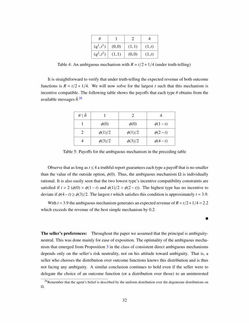
θ 1 2 4

(q1, t1) (0,0) (1,1) (1, t)

(q2, t2) (1,1) (0,0) (1, t)

Table 4: An ambiguous mechanism with R = t/2 + 1/4 (under truth-telling)

It is straightforward to verify that under truth-telling the expected revenue of both outcome

functions is R = t/2 + 1/4. We will now solve for the largest t such that this mechanism is

incentive compatible. The following table shows the payoffs that each type θ obtains from the

available messages θ.28

θ \ θ 1 2 4

1 φ(0) φ(0) φ(1− t)

2 φ(1)/2 φ(1)/2 φ(2− t)

4 φ(3)/2 φ(3)/2 φ(4− t)

Table 5: Payoffs for the ambiguous mechanism in the preceding table

Observe that as long as t≤ 4 a truthful report guarantees each type a payoff that is no smaller

than the value of the outside option, φ(0). Thus, the ambiguous mechanism Ω is individually

rational. It is also easily seen that the two lowest type’s incentive compatibility constraints are

satisfied if t > 2 (φ(0) > φ(1− t) and φ(1)/2 > φ(2− t)). The highest type has no incentive to

deviate if φ(4− t) ≥ φ(3)/2. The largest t which satisfies this condition is approximately t = 3.9.

With t = 3.9 the ambiguous mechanism generates an expected revenue of R = t/2+1/4 = 2.2

which exceeds the revenue of the best simple mechanism by 0.2.

The seller’s preferences: Throughout the paper we assumed that the principal is ambiguity-

neutral. This was done mainly for ease of exposition. The optimality of the ambiguous mecha-

nism that emerged from Proposition 3 in the class of consistent direct ambiguous mechanisms

depends only on the seller’s risk neutrality, not on his attitude toward ambiguity. That is, a

seller who chooses the distribution over outcome functions knows this distribution and is thus

not facing any ambiguity. A similar conclusion continues to hold even if the seller were to

delegate the choice of an outcome function (or a distribution over those) to an uninterested

28Remember that the agent’s belief is described by the uniform distribution over the degenerate distributions onΩ.

32

third party or some mechanical selection device. Ambiguity associated with the behavior of

the third party could never assume payoff relevance as long as all outcome functions yield the

same expected revenue as is required by the consistency condition.

Notice though that the motive for imposing consistency disappears if the choice of the

outcome function (out of an ambiguous mechanism) is not made by the seller himself but is

delegated to an uninterested third party or some mechanical ambiguity device. When the seller

chooses an outcome function (or a distribution over those), then the buyer should assume that

the seller picks the one that is best for himself. Thus, the buyer could only ever perceive the

choice of the outcome function as ambiguous if he thought that the principal was indifferent

over some outcome functions. There is no point in requiring this same indifference condition

when it is not the seller who makes the choice of the outcome function. Therefore, in the case

of an ambiguity averse seller, in principle one would have to consider also non-consistent am-

biguous mechanisms (in combination with the use of external ambiguity devices). Fortunately,

if the seller is a risk neutral maxmin expected utility maximizer, then enlarging the set of ad-

missible ambiguous mechanisms neither changes the value of his problem nor alters the fact

that there must be an optimal ambiguous mechanism among the consistent ones.

Without the requirement that every outcome function in an ambiguous mechanism needs

to yield the same expected revenue Problem P has to be replaced by the following problem:

maxR∈R,Ω⊂XΘ×RΘ

R (P-2)

s.t. R ≤ min(q,t)∈Ω

Ep[t(θ)], (C’)

(DIC), (UIC), (IR).

Note that the only difference between this problem and Problem P is that the constraint (C)

in the latter is replaced by the constraint (C’) in Problem P-2. (C’) represents the fact that the

payoff of a seller who is MMEU ambiguity averse and who delegates the choice of the outcome

function that will be implemented to an external ‘ambiguity device’ (uninterested third party),

is given by the minimum of the expected revenues that the outcome functions in his ambiguous

mechanism generate.

The following result shows that the solutions of Problem P that we have characterized

earlier also solve Problem P-2.

Proposition 6. The ambiguous mechanism generated by the allocation vector Q described in

Proposition 3 solves Problem P-2. That is, it remains an optimal ambiguous mechanism when

the seller has MMEU preferences and one does not require consistency.

33

The intuition for this result is rather straightforward: given that the principal’s payoff is de-

termined by the outcome function that delivers the lowest expected revenue, he might as well

choose to start with a mechanism that contains only outcome functions that yield the same ex-

pected revenue. Suppose we are given a mechanism Ω that does not satisfy this condition. Let

R denote the minimum of the expected revenues of the outcome functions in Ω. By appropri-

ately lowering the transfers of the highest type in all outcome functions who do not produce an

expected revenue of R one can obtain a mechanism that is still downward incentive compatible

and individually rational. By applying Lemmata 1 through 3 this mechanism can be further

transformed to obtain a new mechanism that is also upward incentive compatible and generates

an expected revenue of at least R.

6.3 Surplus extraction: ambiguity aversion vs. risk aversion

In Section 4.4 we have shown that with the use of ambiguous mechanisms the principal can

extract the entire surplus from the agent provided that the agent has MMEU preferences and

his type set is ‘large enough’. This result is related to the findings of Matthews (1983) and

Maskin and Riley (1984) who have studied mechanism design problems with risk averse

agents. Matthews (1983) shows that if the type set is a continuum and the agent has a val-

uation function that exhibits constant absolute risk aversion, then the share of the surplus that

the principal can extract from the agent increases as the agent’s coefficient of absolute risk

aversion increases; in particular, when the agent becomes infinitely risk averse, the principal

can appropriate the entire surplus.

Formally, the case of an ambiguity neutral and risk averse agent with a CARA utility func-

tion resembles the case of an agent who is risk neutral and smoothly ambiguity averse with

a CARA transformation function φ.29 Moreover, the MMEU preferences a la Gilboa and

Schmeidler (1989) that we assume can be seen as the limit of ambiguity averse preferences

that are CARA-smooth, when the CARA coefficient tends to infinity. In the light of these ob-

servations our full rent extraction result for the case where the type set is a continuum, may

seem to be similar to the results in Matthews (1983).

But the analogy between risk aversion and stochastic mechanisms on the one hand and

(smooth) ambiguity aversion and ambiguous mechanisms on the other hand is not quite as

close as it appears at first sight. The central difference between the two cases lies in the fact

that in the case of stochastic mechanisms the distribution of the outcomes is determined by

the designer. That is, the distribution of the outcomes is given by an objective probabilistic

distribution that is a choice variable of the principal. There is no analogous instrument in the

29By the term ‘transformation function’ we mean the function which is applied to transform the expected utilityvalues. It is standard to denote this function by φ as we do in Example 3.

34

case of smooth ambiguity aversion.

Even though in that model uncertainty is described by a distribution (µ) over (distributions

of) outcomes, the higher level distribution (µ)—which is the mathematical analog of the prob-

ability distributions over outcomes in a stochastic mechanism—does not allow for an objective

interpretation.30 In particular, one cannot think of it as a variable that the principal can choose

and can commit to in the way he chooses and commits to the distributions in a stochastic mech-

anism. Instead, the higher level distribution (µ) is only a description of the uncertainty that the

agent perceives and – by the very idea that underlies the concept of uncertainty – there is no

sense in which this perception could be given an objective interpretation as can be done in a

setting with risk aversion by considering only objective probabilistic distribution of outcomes.

Thus, unlike in the case of a stochastic mechanism which fully pins down the perceptions of

the risk averse agent by specifying in an objective way all aspects of the distribution of the out-

comes, an ambiguous mechanism can always just determine the support of the distribution that

describes the agent’s perceptions. All remaining aspects of the agent’s uncertainty perception

are necessarily of a purely subjective nature.

While on the one hand the fact that the higher order distribution in the smooth ambiguity

model describes the subjective uncertainty perceptions of the agent means that it is outside the

direct control of the principal, on the other hand it also implies that it should be considered

as endogenous with respect to the principal’s choices. In particular, this endogeneity of the

agent’s perceptions would call for the use of the consistency concept in an environment with a

smoothly ambiguity averse agent for the same reasons we have adopted it in our setting with

MMEU preferences. Notice that there is no analogous constraint that has to be considered

in a setting with risk aversion and stochastic mechanisms. Thus, the conceptual differences

between the two cases also translate into important differences in their mathematical treatment.

6.4 Consistency

In the design of ambiguous mechanisms we required that all the outcome functions yield the

same ex-ante expected profit, assuming that the buyer reports his type truthfully; we termed

this requirement consistency. Here we provide further insight into why consistency is desirable

and what would be the implications of dropping or weakening the assumption.

Suppose that there were no restrictions on the outcome functions, and suppose the seller

were to announce that the ambiguous mechanism consists of an outcome function that gives the

buyer the good with probability one at the price equal to the type he reported, and an outcome

function that never gives the object to the buyer and never charges him any money. That is, the

30See the discussion of this issue in Klibanoff, Marinacci, and Mukerji (2012).

35

seller announces that he will commit to some randomization over these two outcome functions

but does not reveal the randomization he commits to. If the buyer were to entertain a belief

that contains all distributions over the two outcome functions, he could never expect to get

payoff larger than zero from any of the available reports. Since reporting truthfully would

yield a payoff exactly equal to zero doing so would indeed be optimal for him. However,

foreseeing that the seller would have a strict incentive to choose a randomization that strongly

favors the outcome function that prescribes to transfer the good to the agent at a price equal

to his (trutfully) reported type. Therefore, in a sense, the seller would be fooling the buyer,

or rather, the buyer would be fooling himself by believing that the seller might choose the

outcome function that never gives him the object with a high probability. Consistency serves

to prevent this type of ‘incoherent’ beliefs by the buyer. For more on game theoretic concepts

under ambiguity aversion see also Azrieli and Teper (2011) and Bade (2011).

Rather than requiring that all outcome functions yield the same expected profit one could

try to slightly weaken the consistency assumption. The ideas here are easiest to explain within

an example. Suppose that there are three possible valuations of the buyer, as in the motivating

example, and suppose that the seller offers an ambiguous mechanism consisting of the follow-

ing two outcome functions: (q1, t1) = (1,1), (0,0), (1,4), (q2, t2) = (0,0), (1,2), (1,4). This

mechanism satisfies a weaker requirement that for every outcome function there exists a type

such that the seller would prefer the outcome function if the agent was of that type. In par-

ticular, if the buyer reports truthfully, the seller prefers the first outcome function if the buyer

is the lowest type and the second outcome function if the buyer is the middle type. However,

if the buyer reports truthfully the second outcome function generates a higher expected payoff

than the first, therefore the mechanism does not satisfy the consistency condition. Since the

seller needs to commit to a randomization over the two outcome functions at the beginning, he

would strongly prefer a randomization that attaches a high probability to the second outcome

function. Therefore, this weakening of the consistency assumption results in a similar problem

as dropping the assumption altogether.31

7 Conclusion

In this paper we have studied mechanism design problems where the agent is ambiguity averse

in the sense of Gilboa and Schmeidler (1989). The central insight of our analysis is that the

principal can exploit the agent’s ambiguity aversion by offering ambiguous mechanisms. In

fact, we find that if the type set is ‘large enough’ the designer can extract the entire rent from

the agent.

31We would like to thank a referee for helping us clarify this point.

36

While most of our analysis concentrates on the case of a single agent environment, we

show in Appendix B that when the type distribution is atomless our result readily generalize

to settings with multiple agents. Finally, the core insight of our paper does not depend on the

assumption of MMEU preferences a la Gilboa and Schmeidler (1989). In comparison to other

models of ambiguity aversion, MMEU preferences provide important advantages in terms of

tractability. In Example 3 we have seen that it is optimal for the principal to use ambiguous

mechanisms also if we adopt the less extreme smooth model of ambiguity aversion.

A Appendix

Proof of Proposition 1. Optimality of σ implies

inf(q,t)∈Ω

q(σ(θ))θ− t(σ(θ)) ≥ inf(q,t)∈Ω

q(s)θ− t(s) ∀s ∈ S .

Consider the direct ambiguous mechanism Ω′ defined in the proposition. By the construction

of Ω′ we have

inf(q′,t′)∈Ω′

q′(θ)θ− t′(θ) = inf(q,t)∈Ω

q(σ(θ))θ− t(σ(θ)).

Similarly,

inf(q′,t′)∈Ω′

q′(θ′)θ− t′(θ′) = inf(q,t)∈Ω

q(s′)θ− t(s′)

for s′ = σ(θ′). Combining these three observations yields

inf(q′,t′)∈Ω′

q′(θ)θ− t′(θ) ≥ inf(q′,t′)∈Ω

q′(θ′)θ− t′(θ′) ∀θ′ ∈ Θ,

and so we can conclude that Ω′ is incentive compatible.

That Ω′ is consistent with respect to thruthtelling follows immediately from the fact that Ω

is consistent with respect to σ.

Proof of Lemma 1. Let Ω be a mechanism that satisfies (C), (DIC) and (IR). Let Ω1 be the set

of all simple mechanisms of the form (q, t′), where (q, t) ∈Ω, t′n = tn for all 1 < n < N, and

t′1 = q1θ1 and t′N = tN −p1

pN[t′1− t1].

Since Ω satisfies (IR), t′1 ≥ t1 and t′N ≤ tN . Thus, in passing from t to t′, the transfer of type θ1 is

increased until his truth-telling payoff is zero, while that of θN is lowered so that t and t′ have

37

the same expected value. Since Ω satisfies (C) so does Ω1; in particular, R(Ω) = R(Ω1). By

construction Ω1 satisfies the individual rationality constraint of the lowest type with equality.

Moreover, it is also downward incentive compatible. To see this observe that the truth-telling

payoffs of all types θn, 1 < n < N, are the same under Ω and Ω1. The highest type’s truth-telling

payoff instead is (weakly) larger in Ω1 than in Ω. Regarding the payoffs from downward de-

viations, observe that the only downward deviation report which may deliver different payoffs

in Ω than Ω1 is θ1. But whenever that is the case it is lower in Ω1 than in Ω. Given that the

truth-telling payoffs of types who have downward deviation opportunities are at most higher in

Ω1 than in Ω, it follows that Ω1 must indeed satisfy (DIC) given that Ω does.

Ω1 constitutes the base case for our inductive argument. We next show the inductive step.

Suppose we have defined the mechanisms Ω1, . . . ,Ωn−1 for some 1 < n ≤ N −1. Proceeding in

similar fashion as before, we define Ωn as the set of all simple mechanisms of the form (q, t′),

where (q, t) ∈ Ωn−1, and the transfer rule t′ coincides with t except for the transfers of types θn

and θN , which are

t′n = qnθn− max1≤m<n

inf(q,t)∈Ωn−1

qmθn− tm and t′N = tN −pn

pN[t′n− tn].

Since Ωn−1 satisfies (DIC), it follows that t′n ≥ tn and t′N ≤ tN . The above transformation in-

creases the transfer to be paid upon reporting type θn in all outcome functions until type θn’s

truth-telling payoff from each outcome function becomes equal to the payoff from his most

attractive downward deviation. As before, Ωn inherits the properties (C), (DIC) and (IR) from

Ωn−1; moreover, by construction R(Ωn) = R(Ωn−1).

Finally, define ΩN as the set of all outcome functions of the form (q, t′), where (q, t) ∈ΩN−1

and the transfers t′ coincide with t except for the transfers of the highest type which are set

equal to

t′N = tN + inf(q,t)∈ΩN−1

qNθN − tN− max1≤m<N

inf(q,t)∈ΩN−1

qmθN − tm .

Since ΩN−1 is downward incentive compatible it follows that the difference

inf(q,t)∈ΩN−1

qNθN − tN− max1≤m<N

inf(q,t)∈ΩN−1

qmθN − tm

is non-negative. This means that in passing from ΩN−1 to ΩN the transfers of the highest type

are increased by the same amount in all outcome functions. Thus, property (C) is preserved

and R(ΩN) ≥ R(ΩN−1).

In the first step we have shown that the transfers of the lowest type can be increased so that

each outcome function gives payoff zero to the lowest type when he reports truthfully. The

inductive step then takes an ambiguous mechanism in which the downward incentive compat-

ibility with respect to types θ1 through θn−1 are binding and shows that one can increase the

38

transfers of type θn and decrease the transfers of the type θN so that also type θn’s downward

incentive compatibility constraint becomes binding and the expected transfer of each of the

outcome functions does not change. In the last step the transfers tN in all outcome functions

are uniformly increased until θN’s downward incentive compatibility constraint becomes bind-

ing. ΩN is, therefore, an ambiguous mechanism that satisfies all conditions of (Uni). Thus,

setting Ω′ = ΩN proves the lemma.

Proof of Lemma 2. Let Ω be an ambiguous mechanism that satisfies (C) and (Uni). Denote

its closure (in the usual Euclidean sense) by Ω. Clearly, Ω inherits the properties (C) and (Uni)

from Ω. Moreover, R(Ω) = R(Ω). For each 1 ≤ m < N, let Ωm be the set of outcome functions

in Ω that minimize the probability of the allocation for the report θm:

Ωm = (q, t) ∈ Ω : qm ≤ q′m for all (q′, t′) ∈ Ω. (6)

Let m < n ≤ N. Since θn > θm, an outcome function (q, t) ∈ Ω belongs to Ωm if and only if

(qm − q′m)(θn − θm) ≤ 0 for all (q′, t′) ∈ Ω. By (Uni), qmθm − tm = q′mθm − t′m, hence the above

inequality can be written as qmθn− tm ≤ q′mθn− t′m. It follows that Ωm is also the set of outcome

functions that minimizes the payoff of any type θn > θm when he untruthfully reports θm, that

is, for all m < n ≤ N

Ωm = (q, t) ∈ Ω : qmθn− tm ≤ q′mθn− t′m for all (q′, t′) ∈ Ω. (7)

Define a mechanism Ω by letting (qm, tm) be an arbitrarily chosen element from Ωm, for

m = 1, ...,N − 1. Since, Ω is composed of simple mechanisms that where picked from Ω, it

immediately follows that Ω satisfies (C) and R(Ω) = R(Ω). Moreover, uniformity of Ω implies

that the truth-telling payoffs in Ω must be the same as in Ω, except for possibly the truth telling

payoff of the type θN . For type θN uniformity of Ω requires merely that there is some outcome

function in Ω for which the truth-telling payoff is the same as the highest payoff the agent

obtains in the ambiguous mechanism from misreporting downwards. Ω is obtained from Ω by

pruning some outcome functions. The deletion of outcome functions may lead to an increase

of the payoff of type θN , i.e. it is possible that min(q,t)∈Ω qNθN − tN > min(q′,t′)∈Ω q′NθN − t′N . In

this case we must also have qNθN − tN >max1≤m<N min(q′,t′)∈Ωq′mθN − t′m for all (q, t) ∈ Ω, since

the downward deviation payoffs in Ω and Ω coincide; i.e. Ω may violate the third condition of

(Uni). To deal with this we construct a new ambiguous mechanisms Ω′ from Ω by uniformly

increasing transfers tmN , for m = 1, ...,N − 1, by ∆ = qNθN − tN −max1≤m<N min(q′,t′)∈Ωq

′mθN −

t′m ≥ 0. The fact that all outcome functions in Ω yield the same expected payoff for the seller,

R, implies that all outcome functions in Ω′ yield the expected payoff R′ = R + ∆ ≥ R; i.e. Ω′

39

satisfies (C). Finally, since Ω′ and Ω differ at most in the transfers of the highest type, the

downward deviation payoffs under Ω′ and Ω coincide; the same holds true also for the truth-

telling payoffs of types θn, n = 1, . . . ,N − 1. Ω in turn is composed exactly of those elements

of Ω which define the downward deviation payoffs in Ω. Moreover, as we observed before Ω

inherits from Ω also the truth-telling payoffs of all but possibly the highest type. The fact that

Ω satisfies (Uni) therefore implies that Ω′ must satisfy the first two conditions in the definition

of (Uni). Since it has been constructed to satisfy also the third condition of (Uni), we conclude

that Ω′ satisfies (Uni). Also the property (Min) is obtained by construction.

Proof of Lemma 3. Let Ω = (q1, t1), . . . , (qN−1, tN−1) be a mechanism satisfying (C), (Uni)

and (Min).

We first show that Ω may be changed so that it satisfies the first part of (Mon) while still

satisfying (C), (Uni) and (Min). Consider the mechanism Ω = (q1, t1), . . . , (qN−1, tN−1), where

for each 1 ≤ m < N the allocation rule qm is defined as follows. For every 1 ≤ n ≤ N, qmn = qm

n

if n = m and qmn = 1 otherwise. By construction, Ω satisfies the first part of (Mon). Moreover,

Ω has the same transfer rules as Ω. Given that the latter satisfies (C) so must Ω. For the same

reason we also have R(Ω) = R(Ω). Next, observe that the downward deviation payoffs in Ω and

Ω are the same. Clearly, these payoffs cannot decrease due to the increase in the allocations

that occurs when passing from Ω to Ω (transfers do not change). That they cannot increase

follows from the construction of Ω and the fact that Ω satisfies (Min). Taken together these

properties imply that for all 1 ≤ m < n ≤ N we have

min1≤`<N

q`mθn− t`n = qmmθn− tm

m = qmmθn− tm

m = min1≤`<N

q`mθn− t`n. (8)

Since also the truth-telling payoffs can at most increase, it follows that Ω inherits from Ω

the properties (DIC) and (IR). Applying Lemma 1 to Ω delivers an ambiguous mechanism

Ω = (q1, t1), . . . , (qN−1, tN−1) that satisfies (Uni). Since this last step does not involve any

changes in the allocation rules it follows that Ω satisfies the first part of (Mon), so that for all

1 ≤ m ≤ N − 1 we have qmm ≤ q`m for all 1 ≤ ` ≤ N − 1. In the proof of Lemma 2 we have seen

that this implies that (qm, tm) is the outcome function that defines the payoff from downward

deviations towards θm. We can therefore conclude that Ω satisfies (Min) as well.

We now come to the second part of (Mon). Let Ω = (q1, t1), . . . , (qN−1, tN−1) be a mecha-

nism satisfying (C), (Uni), (Min) and the first part of (Mon). Observe first that if for 1 ≤ m <

m′ < N we have qmm ≤ qm′

m′ then for every type θn, n > m′, a deviation to θm can never be more

attractive than a deviation to θm′ . In order to see this, remember that (Uni) implies (DIC) and

40

so type θm′ must be better off by reporting truthfully than by reporting θm:

qmmθm′ − tm

m ≤ qm′m′θm′ − tm′

m′ . (9)

Then

tm′m′ − tm

m ≤ qm′m′θm′ −qm

mθm′ ≤ (qm′m′ −qm

m)θn

for m′ < n ≤ N. Therefore

qmmθn− tm

m ≤ qm′m′θn− tm′

m′ for all m′ < n ≤ N. (10)

Now assume that Ω does not satisfy the second part of (Mon), and let m′ be the smallest

1 ≤ m < N for which the condition is violated. Thus,

qm′m′ < qm′−1

m′−1 and qmm ≥ qm−1

m−1 ∀ 1 < m < m′. (11)

By our previous observation for every type θn, n >m′−1 the most attractive deviation in the set

θ1, . . . , θm′−1 is θm′−1. Since Ω is uniform this means that the payoff of type θm′ from reporting

truthfully and from reporting θm′−1 is the same, i.e.

qm′−1m′−1θm′ − tm′−1

m′−1 = qm′m′θm′ − tm′

m′ . (12)

But if type θm′ is indifferent between the reports θm′ ant θm′−1, then for each n > m′, type θn

must strictly prefer reporting θm′−1 over reporting θm. Indeed, (12) implies

qm′−1m′−1θn− tm′−1

m′−1 > qm′m′θn− tm′

m′ for all m′ < n ≤ N. (13)

Thus, the downward deviation constraint with respect to θm′m′ cannot be binding for any type θn,

n > m′.

Consider now the mechanism Ω = (q1, t1), . . . , (qN−1, tN−1) that coincides with Ω except

for the values of qm′m′ , tm′

m′ and tm′N . qm′

m′ is increased to qm′−1m′−1, tm′

m′ is increased so that the payoff

that type θm′ gets under the outcome function (qm′ , tm′) when reporting truthfully is the same

one that he gets under the outcome function (qm′ , tm′), i.e.

qm′m′θm′ − tm′

m′ = qm′m′θm′ − tm′

m′ .

Finally, tm′N is chosen such that the expected values of tm′ and tm′ coincide, i.e.

tm′N = tm′

N −pm′

pN

[tm′m′ − tm′

m′].

41

Since tm′m ≥ tm′

m , it follows that tm′N ≤ tm′

N . Notice that in passing from Ω to Ω only the conse-

quences of reporting θm′ and θN under outcome function (qm′ , tm′) are affected. We will argue

now that Ω satisfies all desired properties except possibly the third condition in (Uni) (a binding

downward deviation incentive constraint of type θN). Transfers have been modified in a way

such that the expected value of tm′ remains unchanged. Thus Ω satisfies (C) with R(Ω) = R(Ω).

The truth-telling payoff of type θm′ under (qm′ , tm′) does not change with respect to (qm′ , tm′).

Thus, also in Ω type θm′ gets the same truth-telling payoff from all outcome functions. From

Lemma 2 we know that in combination with qm′m′ ≤ q`m′ , 1 ≤ ` ≤ N−1, this implies that (qm′ , tm′)

defines the payoff from downward deviations toward θm′ by types θn, n > m′. Since no other

downward deviation payoffs could be affected when passing from Ω to Ω, we can conclude that

the latter must satisfy (Min).

The payoffs from downward deviations toward θm′ increase, but they cannot exceed those

from deviations toward θm′−1. To see this, notice that since Ω satisfies (Uni) we have

qm′m′θm′ − tm′

m′ = qm′m′θm′ − tm′

m′ = qm′−1m′−1θm′ − tm′−1

m′−1 = qm′−1m′−1θm′ − tm′−1

m′−1.

Combining this with qm′m′ = qm′−1

m′−1 we get tm′m′ = tm′−1

m′−1. Thus, the payoff that any type can get

from report θm′ under outcome function (qm′ , tm′) coincides with the payoff that he gets from

report θm′−1 under outcome function (qm′−1, tm′−1). Since, the latter defines the payoffs from

downward deviations to θm′−1 the claim follows. We can therefore conclude that Ω satisfies the

first two conditions in (Uni).

As for the third requirement of (Uni) (a binding incentive constraint for downward devia-

tions by the highest type) observe that the truth-telling payoff of type θN may increase since tm′N

decreases. If this is not the case, then Ω satisfies all conditions of (Uni) and so we are done by

setting Ω′ = Ω.

If instead the highest type’s truth-telling payoff is higher in Ω than in Ω, then consider the

mechanism Ω′ which coincides with Ω everywhere except for the transfers of the highest type.

The latter are chosen as follows: for each 1 ≤ m < N, set t′mN = tm

N +ε, where ε is given by

ε = min1≤`<N

q`NθN − t`N− max1≤m<N

min1≤`<N

q`mθm− t`m.

Since in passing from Ω to Ω′ the highest type’s transfer is increased uniformly across all

outcome functions it follows that Ω′ satisfies (C) with R(Ω′) > R(Ω). Moreover, the fact that

by the switch from Ω to Ω′ only the transfers for the highest type are affected, implies that

Ω′ inherits both (Min) and the first two parts of (Uni) from Ω. Finally, in Ω′ the transfers of

the highest are chosen exactly such that the highest type’s downward deviation constraint is

binding. Consequently, Ω′ satisfies all parts of (Uni) and so the proof is complete.

42

Proof of Lemma 4. Let Ω be a mechanism that satisfies (Uni), (Min) and (Mon). Let N > n >

m ≥ 1. Then

min(q,t)∈Ω

qnθm− tn ≤ qnnθm− tn

n

= qnn(θm− θn) + qn

nθn− tnn = qn

n(θm− θn) + qn−1n−1θn− tn−1

n−1

= qnn(θm− θn) + qn−1

n−1(θn− θn−1) + qn−1n−1θn−1− tn−1

n−1...

...

= qnn(θm− θn) + qn−1

n−1(θn− θn−1) + . . .+ qmm(θm+1− θm) + qm

mθm− tmm

= qmmθm− tm

m −

n−m−1∑k=0

(qn−kn−k −qn−k−1

n−k−1)(θn−k − θm)

≤ qmmθm− tm

m

= min(q,t)∈Ω

qmθm− tm.

The first inequality is definitional, the second inequality follows from the fact that qnn is non-

decreasing in n and the last equality is implied by (Uni). The equalities between the two

inequalities follow from the fact that for each 1 < n ≤ N, the binding downward incentive

constraint of type θn, is the one with respect to the adjacent lower type θn−1. This has been

shown in the proof of Lemma 3, where we have seen that in a uniform ambiguous mechanism

(one of) the binding incentive constraint for downward deviations for type θn, 1 < n < N, is the

one with respect to type θmn , where

mn ∈ arg max1≤m<n

min

1≤`<Nq`m

.

For a mechanism that is also minimal and monotonic it thus follows that mn = n−1.

In the preceding argument we do not allow for n = N. The reason for this is purely nota-

tional. A perfectly analogous argument can be applied in the case n = N by using in the first row

instead of (qn, tn) the mechanism that minimizes the truth telling payoff of the highest type.

Proof of Proposition 2. By Lemma (4) we know that every mechanism that is feasible in Prob-

lem P’ also satisfies (UIC). It also satisfies (DIC) and (IR) because it satisfies (Uni); see the

paragraph after Definition 4. Therefore every such mechanism is feasible in Problem P and

thus the value of Problem P cannot be smaller than the value of Problem P’.

On the other hand, Lemmata 1 through 3 imply that for every mechanism that is feasible

in Problem P there exists a mechanism with at least as high an expected revenue for the seller,

that is feasible in Problem P’. But then the value of Problem P’ must be at least as large as the

value of Problem P.

43

Proof of Lemma 5. If Ω satisfies (Uni), (Min) and (Mon), then for each 1 < n ≤ N the binding

downward incentive constraint of type θn is the one with respect to θn−1 (see the proof of

Lemma 3). Thus,

tm1 = qm

1 θ1 for all 1 ≤ m < N, (14)

tmn+1 = (qm

n+1−qnn)θn+1 + tn

n for all 1 ≤ n ≤ N −2 and 1 ≤ m < N,

tmN ≤ (1−qN−1

N−1)θN + tN−1N−1, for all 1 ≤ m < N.

From this it is straightforward to derive (3) and (4) by recursively substituting the expressions

tnn into the formula for tm

n+1.

Conversely, suppose we are given a minimal and monotonic mechanism Ω the transfers

of which satisfy (3) and (4). It is then easily verified that for each 1 ≤ n < N the truth-telling

payoffs of type θn are constant across outcome functions. This in turn implies that the payoff

type θn, n≤ N, obtains from a deviation to θm, 1≤m< n, is determined by the outcome function

(qm, tm) (since this is the outcome function that minimizes the allocation probability after report

θm). Using this it is straightforward to show that the payoff of type θn from deviating to θm,

m < n is increasing in m and is equal to the truthtelling payoff for m = n−1. With other words,

type θn’s downward adjacent IC constraint is binding.

In order to see this, consider the difference in the payoff of type θn from reporting θm and

θm−1, m ≤ n.

min1≤l<N

qlmθn− tl

m− min1≤l<N

qlm−1θn− tl

m−1 = qmmθn− tm

m −qm−1m−1θn− tm−1

m−1 (15)

= qmmθn−qm

mθm +

m−1∑k=1

qkk(θk+1− θk)−qm−1

m−1θn + qm−1m−1θm−1−

m−2∑k=1

qkk(θk+1− θk) (16)

= (θn− θm)(qmm−qm−1

m−1) ≥ 0. (17)

Given that qmm ≥ qm−1

m−1 this difference is non-negative. Moreover, it becomes zero for m = n.

Hence, Ω satisfies all downward incentive constraints and the one with respect to the adjacent

lower type is binding. Combining all these observations we can conclude that Ω satisfies (Uni).

Starting with Lemma 6 all results from Section 4.3 are stated using Assumption 1. Since

the only role of Assumption 1 was to simplify the exposition in the main text in what fol-

lows we state and prove versions of the results that do not rely on this assumption. In order

to do so we introduce some further notation. First, we inductively construct the set M =

m1, . . . ,mM,mM+1, which is a subset of the index set N. The first element, m1, is set equal to

1. If for m j−1 the set n : N > n >m j−1, pnθn > pm j−1θm j−1 is non-empty, we set m j = minn : N >

44

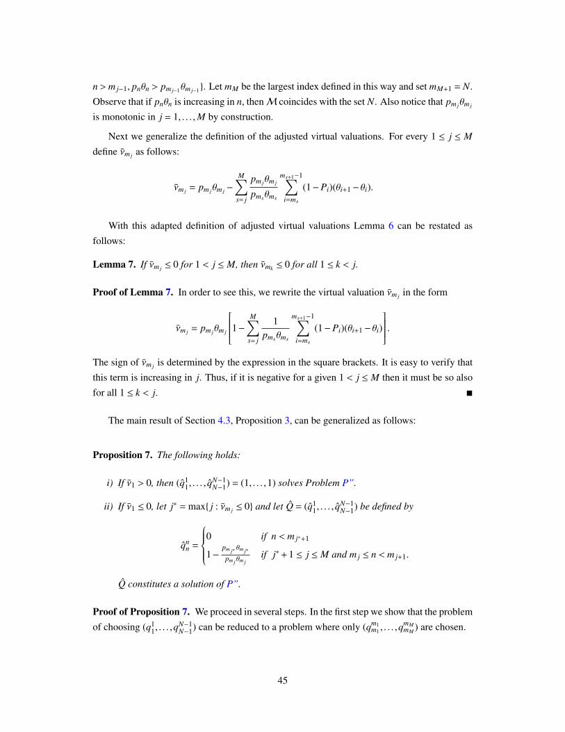
n >m j−1, pnθn > pm j−1θm j−1. Let mM be the largest index defined in this way and set mM+1 = N.

Observe that if pnθn is increasing in n, thenM coincides with the set N. Also notice that pm jθm j

is monotonic in j = 1, . . . ,M by construction.

Next we generalize the definition of the adjusted virtual valuations. For every 1 ≤ j ≤ M

define νm j as follows:

νm j = pm jθm j −

M∑s= j

pm jθm j

pmsθms

ms+1−1∑i=ms

(1−Pi)(θi+1− θi).

With this adapted definition of adjusted virtual valuations Lemma 6 can be restated as

follows:

Lemma 7. If νm j ≤ 0 for 1 < j ≤ M, then νmk ≤ 0 for all 1 ≤ k < j.

Proof of Lemma 7. In order to see this, we rewrite the virtual valuation νm j in the form

νm j = pm jθm j

1− M∑s= j

1pmsθms

ms+1−1∑i=ms

(1−Pi)(θi+1− θi)

.The sign of νm j is determined by the expression in the square brackets. It is easy to verify that

this term is increasing in j. Thus, if it is negative for a given 1 < j ≤ M then it must be so also

for all 1 ≤ k < j.

The main result of Section 4.3, Proposition 3, can be generalized as follows:

Proposition 7. The following holds:

i) If ν1 > 0, then (q11, . . . , q

N−1N−1) = (1, . . . ,1) solves Problem P”.

ii) If ν1 ≤ 0, let j∗ = max j : νm j ≤ 0 and let Q = (q11, . . . , q

N−1N−1) be defined by

qnn =

0 if n < m j∗+1

1−pm j∗ θm j∗

pm jθm jif j∗+ 1 ≤ j ≤ M and m j ≤ n < m j+1.

Q constitutes a solution of P”.

Proof of Proposition 7. We proceed in several steps. In the first step we show that the problem

of choosing (q11, . . . ,q

N−1N−1) can be reduced to a problem where only (qm1

m1 , . . . ,qmMmM ) are chosen.

45

Step 1. If m j < n < m j+1, 1 ≤ j ≤ M, then at the optimum qnn = qm j

m j .

In order to see this observe that since for every Q with non-decreasing components, we

have qnn ≥ qm j

m j it follows that

Rn(Q)− Rm j(Q) = −pnθn(1−qnn) + pm jθm j(1−qm j

m j) ≥ (1−qm jm j)(pm jθm j − pnθn) ≥ 0.

That is, there is no admissible Q for which Rn(Q) is the (strictly) smallest upper bound on the

revenues. But Rn(Q) is the only bound that could be increasing in qnn. Thus, it is without loss

to choose qnn as small as possible, i.e. we can set qn

n = qn−1n−1. Since this argument applies to all

m j < n < m j+1 we can conclude that choosing qnn = qm j

m j for all m j < n < m j+1 is optimal.

Step 2. At the optimum

qm j+1m j+1 ≤ 1−

pm jθm j

pm j+1θm j+1

(1− qm jm j)

for all 1 ≤ j ≤ M−1.

In order to see this, notice that for every Q such that

qm j+1m j+1 > 1−

pm jθm j

pm j+1θm j+1

(1−qm jm j)

we have

Rm j+1(Q)− Rm j(Q) > 0.

Moreover, rewriting the inequality yields

qm j+1m j+1 −qm j

m j >

(1−

pm jθm j

pm j+1θm j+1

)(1−qm j

m j) ≥ 0.

In such a case we can lower qm j+1m j+1 without violating the constraint qm j+1

m j+1 ≥ qm jm j , and thus increase

all Rn, n , m j+1. Since Rm j+1 is not the smallest bound this means that the minimum of the

bounds would increase. But then Q cannot be optimal.

Step 3. If ν1 ≤ 0 then at the optimum

qm jm j = 1−

pm j−1θm j−1

pm jθm j

(1− qm j−1m j−1) for all j∗ < j ≤ M;

if ν1 > 0 then this condition holds for all 1 < j ≤ M.

By Step 2 we know that at the optimum

qm jm j ≤ 1−

pm j−1θm j−1

pm jθm j

(1− qm j−1m j−1),

46

for all 1 < j ≤ M or equivalently

Rm j(Q) ≤ Rm j−1(Q).

Now suppose that Q is such that this condition holds with strict inequality for j = M, implying

qmMmM < 1. Then, RmM (Q) is strictly smaller than any other bound. If Q is optimal then it should

not be possible to increase RmM . An increase of RmM can be achieved only if qmMmM is increased.

On the other hand, since for all mM < n < N we have qnn = qmM

mM , qmMmM can be increased without

violating monotonicity only if at the same time we also increase qnn for mM < n< N. The impact

of a uniform increase of (qmMmM , . . . ,q

N−1N−1) on RmM is

pmMθmM −

N−1∑i=mM

(1−Pi)(θi+1− θi) = νmM .

Thus Q cannot be optimal if νmM > 0. This proves the claim for j = M > j∗.

For the case that j lies strictly between j∗ and M (i.e. j∗ < j < M) assume that we have

shown the claim for s = j + 1, . . . ,M. If Q is such that

qm jm j < 1−

pm j−1θm j−1

pm jθm j

(1− qm j−1m j−1)

then

RmM (Q) = . . . = Rm j+1(Q) = Rm j(Q) < Rm j−1(Q) ≤ . . . ≤ Rm1(Q).

The assumption that the claim holds for s = j + 1, . . . ,M implies that

qmsms = 1−

pms−1θms−1

pmsθms

(1−qms−1ms−1) = 1−

pms−1θms−1

pmsθms

[1−

(1−

pms−2θms−2

pms−1θms−1

(1−qms−2ms−2)

)]=

pms−2θms−2

pmsθms

(1−qms−2ms−2) = . . .

= 1−pm jθm j

pmsθms

(1−qm jm j).

Moreover, by Step 1 we know that for ms−1 < n < ms, s = j + 1, . . . ,M,

qnn = qms−1

ms−1 .

Thus, if starting from Q we want to increase qm jm j , then monotonicity combined with the fact

that the claim holds for all s = j + 1, . . . ,M implies that we must increase qnn, ms−1 ≤ n < ms,

47

s = j + 1, . . . ,M, at the rate

pm jθm j

pms−1θms−1

.

If (qm jm j , . . . ,q

N−1N−1) is increased in this way then Rm j changes at the rate

pm jθm j −

M∑s= j

pm jθm j

pmsθms

ms+1−1∑i=ms

(1−Pi)(θi+1− θi) = νm j .

Thus, if νm j > 0, then Q cannot be optimal.

Step 4. If ν1 ≤ 0 then at the optimum qm jm j = 0 for all j ≤ j∗.

Consider first the case j = j∗. From Step 3 we know that for all s = j∗ + 1, . . . ,M the

condition

qmsms = 1−

pm j∗ θm j∗

pmsθms

(1− qm j∗

m j∗) (18)

holds. Thus, varying qm j∗

m j∗implies that we have to change accordingly also all qn

n, m j∗ < n < N.

In the previous step we have seen that the overall effect that such a change has on Rm j∗ is

measured by νm j∗ . Therefore, since νm j∗ ≤ 0, Rm j∗ is maximized by choosing qm j∗

m j∗as small as

possible. But that means that we have to set qm j∗

m j∗= q

m j∗−1m j∗−1

.

Next, consider the choice of qm j∗−1m j∗−1

. If qm j∗

m j∗= q

m j∗−1m j∗−1

, then

Rm j∗ (Q)− Rm j∗−1(Q) = (1−qm j∗−1m j∗−1

)(pm j∗−1θm j∗−1 − pm∗jθm∗j ). (19)

If qm j∗−1m j∗−1

< 1 this expression is strictly negative, meaning that Rm j∗−1 is not the smallest one of

the bounds. Since all other bounds are strictly decreasing in qm j∗−1m j∗−1

, so must be min j Rm j . Hence,

qm j∗−1m j∗−1

must be chosen as small as possible. If qm j∗

m j∗= q

m j∗−1m j∗−1

= 1, then Rm j∗−1 can be increased by

a decrease of qm j∗−1m j∗−1

that is accompanied with a reduction of all qnn, m j∗−1 < n< N, in accordance

with (18). In order to see this notice that by (19) we know that in the initial situation we have

Rm j∗ = Rm j∗−1 . After the proposed reduction of all qnn, m j∗−1 ≤ n < N instead we have Rm j∗ <

Rm j∗−1 . By our previous arguments we know that a reduction of (qm j∗

m j∗, . . . ,qN−1

N−1) in accordance

with (18) leads to an increase of Rm j∗ and min j Rm j . If in addition also (qm j∗−1m j∗−1

, . . . ,qm j∗−1m j∗−1)

is reduced then certainly Rm j , j , j∗ − 1, increase further. Moreover, since after the change

Rm j∗ < Rm j∗−1 it must be the case that also Rm j∗−1 increases. Combining these arguments we

conclude that qm j∗−1m j∗−1

must be chosen as small as possible, i.e. qm j∗−1m j∗−1

= qm j∗−2m j∗−2

.

Iterating on the same argument we can show that for all m j ≤ m j∗ , qm jm j must be chosen as

small as possible. Since for m1 this means qm1m1 = 0 we thus get qm j

m j = 0 for all m j ≤ m j∗ .

48

Step 5. If ν1 > 0, then at the optimum qm jm j = 1 for all 1 ≤ j ≤ M.

In Step 3 we have seen that if νm j > 0 for all j∗ < j ≤ M then each qm jm j has to be chosen as

large as the constraint

qm jm j ≤ 1−

pm j−1θm j−1

pm jθm j

(1− qm j−1m j−1) (20)

allows. Since there is no such constraint for j = 1 it follows that qm1m1 must be optimally set

equal to 1. Monotonicity then requires that also qnn, 1 < n < N −1, must be equal to 1.

Proof of Proposition 4 . In the text we explained what happens when an offer for θ1 is the

optimal simple mechanism. Here we assume it is not. An optimal simple mechanism (q, t) is

then an offer at a price equal to one of the types above θ1, that is, there is a n > 1 such that

qn = 0 for all n < n and qn = 1 for all n ≥ n. We will show that for each such mechanism one can

find an ambiguous mechanism that generates a strictly larger expected revenue to the seller.

Fix an optimal simple mechanism (q, t) as described above, and define the ambiguous

mechanism Ω(n,q) = (q1, t1), . . . , (qN−1, tN−1) as follows

qmn =

0 if n = m and n < n

q if n = m and n ≥ n

1 else,

tmn =

qm

n θn if n = m

θn if n , m and n < n

(1−q)θn + qθn if n , m and n ≥ n,

where q ∈ [0,1]. Notice that there is nothing in the definition of Ω(n,q) that guarantees consis-

tency. We will deal with that condition in a second step.

Next we show now that there exists a value q such that under truth-telling each of the

outcome functions of Ω(n, q) generates an expected revenue that strictly exceeds the expected

revenue achieved by an optimal simple mechanism. To see this, notice that under truth-telling

the m-th outcome function of Ω(n,q) yields an expected revenue

Rm(Ω(n,q)) =

∑

n<n, n,m pnθn +∑

n≥n pn[(1−q)θn + qθn] if m < n,∑n<n pnθn + pmqθn +

∑n≥n, n,m pn[(1−q)θn + qθn] else.

(21)

The revenue of the take-it-or-leave-it-offer for θn (an optimal simple mechanism) is

R = θn

∑n≥n

pn. (22)

49

Comparing the expressions (21) and (22) reveals that for all m < n the former is strictly larger

than the latter for all q ∈ (0,1). As for the case m ≥ n observe that

Rm(Ω(n,q))− R =∑n<n

pnθn− pm(1−q)θn +∑

n≥n,n,m

pn(1−q)(θn− θn).

Since∑

n<n pnθn > 0 this difference must be strictly positive for q close to 1. Thus, when q is

close enough to 1

Rm(Ω(n,q)) > R

for all m. Fix a q < 1 that satisfies this inequality and label it q. We next modify Ω(n, q) such

that it satisfies consistency while still achieving an expected revenue equal to

minm′

Rm′(Ω(n, q)) > R.

To do so define

∆m = Rm(Ω(n, q))−minm′

Rm′(Ω(n, q))

and manipulate the transfers of the highest type in all outcome functions of Ω(n, q) by subtract-

ing ∆m, i.e. set

tmN = tm

N −∆m.

Denote the ambiguous mechanism obtained after the change in the highest type’s transfers by

Ω(n, q).

By construction all outcome functions of Ω(n, q) yield the same expected revenue and this

expected revenue is strictly larger than the revenue of the optimal simple mechanism. It is

straightforward to verify that Ω(n, q) is constructed in such way that it satisfies the properties

(Uni), (Min) and (Mon). Lemma 4 therefore implies that Ω(n, q) is incentive compatible. Thus,

Ω(n, q) is a Problem-P’-feasible mechanism that produces a larger expected revenue than the

best simple mechanism.

In order to complete the proof we need to argue that Q = (1, . . . ,1) not being a solution of

P” is equivalent to ν1 < 0. Proposition 3 implies that when ν1 > 0, Q = (1, . . . ,1) is a solution

to P”. On the other hand, step 4 of the proof of Proposition 3 states that if ν1 ≤ 0, then at the

optimum qm jm j = 0 for all j ≤ j∗. It is easy to see from the proof that when ν1 < 0, Q = (1, . . . ,1)

cannot be a solution to P”. However, when ν1 = 0, there can be other solutions beside the one

in the statement of Proposition 3. In that case R1(Q), as used in the proof, is constant when one

varies q11 and adjusts the other qm j

m j as in the said proof. Thus setting Q to (1, . . . ,1) does not

affect R1(Q) and provides an upper bound on the expected profit for the seller. In addition, for

Q = (1, . . . ,1), Rm j is constant in m j, and in particular equal to θ1. Therefore the upper bound is

50

attained, and Q = (1, . . . ,1) is also a solution. To conclude, Q = (1, . . . ,1) is not a solution to P”

if and only if ν1 < 0.

Proof of Proposition 6. Consider the relaxed versions of Problem P-2 from which (UIC) has

been dropped. Suppose that Ω is a feasible mechanism of that problem and that (q, t) is one

of the simple mechanisms in Ω that generates the smallest expected revenue, i.e. (q, t) ∈

argmin(q,t)∈ΩEp[t(θ)].

Let Ω′ be the set of all outcome functions of the form (q, t′), where (q, t) ∈Ω and the transfer

rule t′ coincides with t except for the transfers of the highest type, which are equal to

t′N = tN −[Ep[t(θ)]−Ep[t(θ)]

]/pN .

Ω′ inherits from Ω the properties (IR) and (DIC). This follows from the fact that in passing

from Ω to Ω′ only the highest type’s transfers are lowered. Thus, both individual rationality

and downward incentive compatibility can at most be relaxed. Moreover, by construction we

have that

Ep[t(θ)] =Ep[t(θ)] for all (q, t) ∈Ω′.

Thus, Ω′ satisfies (C) and generates the same value as Ω. But that means that the value of the

relaxed version of Problem P-2 does not change if the constraint (C’) is replaced by (C). Doing

so yields the relaxed version of Problem P. We already know that the latter has the same value

as Problem P itself.

Proof of Proposition 8. Consistency follows from the fact that any two simple mechanisms in

Ω differ only on a set of types with zero probability. Notice also that every simple mechanism

almost always awards the object to the agent with the higher announced type at a price that is

equal to the announced type. Thus, under truth telling each simple mechanism in Ω generates

a revenue of T =E[maxθ1, θ2].

As for individual rationality observe that the ambiguous mechanism never specifies a pay-

ment for an agent unless he receives the object. When an agent receives the object, then he

has to make a payment that corresponds to his announced valuation. Thus, truth telling always

guarantees a non-negative payoff.

Finally, we have to argue that under Ω truth telling is an optimal strategy for the two agents,

irrespective of what they believe about the other agent’s type or play. In order to see this, notice

that for every profile of announced types, θ, agent i knows that there are simple mechanisms in

Ω (all those indexed by a type profile, θ, such that θi = θi) that specify that he will not receive

51

the object and that he will not have to pay anything. This means that for every θ his payoff is

at most zero. On the other hand, by revealing his type truthfully, agent i can never get a strictly

negative payoff since every outcome function specifies for every pair of reported types one of

two possible outcomes for agent i: either he gets the object with probability one and pays the

reported valuation or he does not get the object and pays zero; in either case the resulting payoff

is zero.

B Appendix

In the main text we have restricted our attention to optimal mechanism design problems in

single agent environments. In this section we show how the full surplus extraction result of

Corollary 3 can be extended to a setting with multiple agents.32 More specifically, in what

follows we consider a setting with two agents whose types are drawn from an atomless dis-

tribution. The assumption of two agents is made for notational convenience only. All the

arguments easily extend to the case with more than two agents.

Assume that the two agents have preferences as in the previous sections. We denote the

type set of agent, i = 1,2, by Θi. For a generic element of this set we write θi; generic type

profiles in Θ = ×iΘi, are indicated by θ. We assume that the agents’ types are (independently)

drawn from the atomless distribution p with support [0,1]. We do not need to assume that the

designer knows the exact type distribution. For the following result we only need to impose

that he knows the support of the distribution. Regarding the two agents’ beliefs about each

others type distribution we make no assumptions at all.

Proposition 8 (Full surplus extraction with multiple agents). Consider a two agent setting as

described in the preceding paragraph. Moreover, let the ambiguous mechanism Ω = (qθ, tθ) :

θ ∈ Θ, be defined by

qθ(θ) =

(0,0) if θ = θ

(1,0) if[θ1 , θ1 and θ2 = θ2

]or

[θ1 , θ1, θ2 , θ2, and θ1 ≥ θ2

](0,1) else

tθ(θ) = (qθ1(θ)θ1,qθ2(θ)θ2).

Under Ω truth-telling is an optimal strategy for the two agents irrespective of their beliefs

regarding the other agent’s type or play. Moreover, Ω is individually rational and consistent32The following full-rent-extraction result for multiple agents implies that ambiguous mechanisms outperform

simple mechanisms also in situations with multiple agents. For a characterization of expected revenue maximizingsimple mechanisms in general environments see Kos and Messner (2013a) and Kos and Messner (2013b).

52

(with respect to truth telling). The expected revenue generated by each element of Ω is T =

E[maxθ1, θ2]. That is, Ω achieves full surplus extraction.

The ambiguous mechanisms presented in the above result can be constructed as follows.

For every profile of types θ = (θ1, θ2) we add to the ambiguous mechanism a simple mechanism

(qθ, tθ) with the following property. If both agents’ reports coincide with the corresponding

component of the label of the simple mechanism, i.e. if for every i we have θi = θi, then the

seller keeps the object and there are no transfers. If, neither agent’s report coincides with label,

i.e. if for every i, θi , θi, then the agent with the higher report receives the object at the price he

reported. Finally, if only one agent’s report coincides with the label of the simple mechanism,

then the agent whose report does not coincide receives the object at the price equal to the value

he announced. Since the ambiguous mechanism contains all such simple mechanisms, there

is a simple mechanism for each report of each agent such that the agent does not receive the

object if he reports that type. This bounds the agent’s expected payoff above by 0. By reporting

truthfully the agent either obtains the object and pays the reported, and therefore true, value or

does not receive it and pays zero. In either case the agent’s payoff is zero, which is also the

before established upper bound. But then the agent has no incentives to deviate from truthful

reporting. This establishes that truthful reporting is an equilibrium of the proposed mechanism.

On the other hand, assuming that the agents do report truthfully and that each profile of types

occurs with probability zero, each simple mechanism yields for the seller the expected surplus

E[maxθ1, θ2]. With other words, the seller extracts the full surplus.

References

Ashenfelter, Orley (1989), “How auctions work for wine and art.” The Journal of Economic

Perspectives, 23–36.

Auster, Sarah (2015), “Robust contracting under common value uncertainty.” Working Paper.

Azrieli, Yaron and Roee Teper (2011), “Uncertainty aversion and equilibrium existence in

games with incomplete information.” Games and Economic Behavior, 73, 310–317.

Bade, Sophie (2011), “Ambiguous act equilibria.” Games and Economic Behavior, 71, 246–

260.

Bajari, Patrick and Ali Hortacsu (2003), “The winner’s curse, reserve prices, and endogenous

entry: empirical insights from ebay auctions.” RAND Journal of Economics, 329–355.

Bergemann, D. and S. Morris (2005), “Robust mechanism design.” Econometrica, 73, 1521–

1534.

53

Bergemann, D. and K. Schlag (2011), “Robust monopoly pricing.” Journal of Economic The-

ory, 146, 2527–2543.

Bergemann, Dirk and Johannes Horner (2010), “Should auctions be transparent?” Working

Paper.

Bodoh-Creed, Aaron (2012), “Ambiguous beliefs and mechanism design.” Games and Eco-

nomic Behavior, 75, 518–537.

Bose, Subir and Arup Daripa (2009), “A dynamic mechanism and surplus extraction under

ambiguity.” Journal of Economic Theory, 144(5), 2084–2114.

Bose, Subir, Emre Ozdenoren, and Andreas Pape (2006), “Optimal auction with ambiguity.”

Theoretical Economics, 1, 411–438.

Bose, Subir and Ludovic Renou (2014), “Mechanism design with ambiguous communication

devices.” Econometrica, 82, 1853–1872.

Castro, L. De and N.C. Yannelis (2012), “Uncertainty, efficiency and incentive compatibility.”

Unpublished manuscript.

Chung, K.S. and J. Ely (2007), “Foundations of dominant strategy mechanisms.” Review of

Economic Studies, 74, 447–476.

Ellsberg, Daniel (1961), “Risk, ambiguity, and the savage axioms.” Quarterly Journal of Eco-

nomics, 75 (4), 643–669.

Elyakime, B., J.J. Laffont, P. Loisel, and Q. Vuong (1994), “First price sealed-bid auctions with

secret reservation prices.” Annales d’Economie et de Statistique, 34, 115–141.

Epstein, Larry and Martin Schneider (2008), “Ambiguity, information quality and asset prices.”

Journal of Finance, 63(1), 197-228., 197–228.

Garrett, D.F. (2014), “Robustness of simple menus of contracts in cost-based procurement.”

Games and Economic Behavior, 87, 631–641.

Gilboa, Itzhak (2009), Theory of Decision Under Uncertainty. Cambridge University Press.

Gilboa, Itzhak and Massimo Marinacci (2016), “Ambiguity and the bayesian paradigm.” In

“Readings in Formal Epistemology,” Springer, pp. 385–439.

Gilboa, Itzhak and David Schmeidler (1989), “Maxmin expected utility with a non-unique

prior.” Journal of Mathematical Economics, 18, 141–153.

54

Hendricks, Kenneth, Robert H Porter, and Richard H Spady (1989), “Random reservation

prices and bidding behavior in ocs drainage auctions.” JL & Econ. S83, 32.

Kellner, M. (2015), “Tournaments as response to ambiguity aversion in incentive contracts.”

Journal of Economic Theory, 159(A), 627–655.

Klibanoff, P., M. Marinacci, and S. Mukerji (2012), “On the smooth ambiguity model: A reply.”

Econometrica, 80(3), 1303–1321.

Klibanoff, Peter, Massimo Marinacci, and Sujoy Mukerji (2005), “A smooth model of decision

making under ambiguity.” Econometrica, 73, 1849–1892.

Kos, Nenad and Matthias Messner (2013a), “Extremal incentive compatible transfers.” Journal

of Economic Theory, 148, 134–164.

Kos, Nenad and Matthias Messner (2013b), “Incentive compatibility in non-quasilinear envi-

ronments.” Economics Letters, 121, 12–14.

Kos, Nenad and Matthias Messner (2015), “Selling to the mean.” Technical report, CESifo

Working Paper.

Lang, Matthias and Achim Wambach (2013), “The fog of fraud - mititigating fraud by strategic

ambiguity.” Games and Economic Behavior, 81, 255–275.

Lopomo, Giuseppe, Luca Rigotti, and Chris Shannon (2009), “Uncertainty in mechanism de-

sign.” Working paper.

Maskin, Eric and John Riley (1984), “Optimal auctions with risk averse buyers.” Econometrica,

52, 1473–1518.

Matthews, Steven (1983), “Selling to risk averse buyers with unobservable tastes.” Journal of

Economic Theory, 30, 370–400.

Raiffa, H. (1961), “Risk, ambiguity, and the savage axioms: Comment.” Quarterly Journal of

Economics, 75, 690–694.

Saito, Kota (2015), “Preferences for flexibility and randomization under uncertainty.” The

American Economic Review, 105, 1246–1271.

Szydlowski, Martin (2012), “Ambiguity in dynamic contracts.” SSRN Working Paper

http://ssrn.com/abstract=1986186.

Turocy, Theodore L. (2008), “Auction choice for ambiguity-averse sellers facing strategic un-

certainty.” Games and Economic Behavior, 62, 155–179.

55

Wolitzky, Alexander et al. (2014), “Mechanism design with maxmin agents: theory and an

application to bilateral trade.” manuscript, Stanford University.

56