Y

X

The derivative

Lecture 5Handling a changing world

Y

X

x2-x1

y2-y1

The derivative

x2-x1

y2-y1

xy

xxyy

slope

12

12

xxfxxf

xxxfxf

slope

)()()()( 11

12

12

x1 x2

y1

y2

xxfxxf

slope x

)()(lim 0

xxfxxf

yxfdxdy

x

)()(lim)(' 0

The derivative describes the change in the slope of functions

Aryabhata (476-550)

Bhaskara II (1114-1185)

The first Indian satellite

-10

-5

0

5

10

-4 -2 0 2 4

YX

)()(

)( ufbudxxdf

bauuy

u

0)2(

2

2)2(

bdxxdf

bay

( * ) ' '* * 'f g f g f g ( ( )) ' '* 'f g f g

( ) ' ' '

( ) ' ' '

f g f g

f g f g

'

2

'* * 'f f g f g

g g

Four basic rules to calculate derivatives

b

Local minimum

0)(

dxxdf Stationary point,

point of equilibrium)('

)()(cf

abafbf

Mean value theorem

0

1

2

3

0 5 10 15 20

Y

X

05

10152025303540

0 5 10 15 20

Y

X

Dy=30-10

Dx=15-5

25101030

lim 0

xy

dxdy

x

The derivative of a linear function y=ax equals its slope a

xy 2

Dy=0

0lim 0 xy

dxdy

x

The derivative of a constant y=b is always zero. A constant doesn’t change.

2y

aybaxy '

0

5

10

15

20

25

30

0 1 2 3 4

Y

X

xx edxdy

ey

dy

dx

xeydxdy

The importance of e

ax

x exa

1lim

ex

x

x

11lim

)ln(xy

xedxdy

edydx

dydxdxdy

exxy

yy

y

11

/1

)ln(

-2

-1

0

1

2

3

4

0 1 2 3 4

Y

X

)ln(xy xy

1

1)ln()ln()ln()ln(

)ln()ln(

)1

)ln(00())'ln()(ln(''

bbxbaxbau

uxbab

abxxb

axxbxexbaeuey

eeaxy

baxy

xxxxu

ubxax

bbababxbabbxaabuey

eeaby

)ln()ln()0)ln(10())'ln()(ln(''

)ln()ln(

xaby

xx

xx

xxxxxy

xxxx

y

xx

x

)sin(lim)cos(

)sin()sin()cos()cos()sin(lim'

)sin()sin(lim'

00

0

)sin(xy

)cos()(sin'1)sin(

lim 0 xxxx

x

)sin()(cos' xx

The approximation of a small increase

xxfxfxxfx

xxfxfxxfx

xfxxfslope

xx

x

x

)('lim)()(lim

0)(')()(

lim

)()(lim

00

0

0

How much larger is a ball of 100 cm radius if we extend its radius to 105 cm?

3233 628.0)1(405.0 mmmV

The true value is DV = 0.66m3.

23 4'34

rVrV

012345678

-4 -2 0 2 4

Y

X

xee

yxx

x

0lim

Rule of l’Hospital

2111

)0(1

'

)(;)(lim 0

yee

y

xxgeexfxee

y

xx

xxxx

x

)()()(

)(

)()()(

)(

0

0

xxdxxdg

dxdxxdg

xg

xxdxxdf

cxdxxdf

xf

)()(

)( 00 xxdxxdf

xf

The value of a function at a point x can be approximated by its tangent at x.

)(')('

)()(

)()(

)()(

0

0

xgxf

cxdxxdg

cxdxxdf

xgxf

)(')('

lim)()(

limxgxf

xgxf

axax

0)(lim)(lim00

xgxf xxxx

0

5

10

15

20

25

30

-2 -1 0 1 2 3 4 5

Y

X

-25

-20

-15

-10

-5

0

5

-2 -1 0 1 2 3 4 5

Y

X

-20-15-10-505

101520

-2 -1 0 1 2 3 4 5Y

X

Stationary points

Minimum MaximumHow to find minima and maxima of functions?

0

5

10

15

20

25

30

-2 -1 0 1 2 3 4 5

Y

X

f’<0f’>0 f’<0

f’=0

f’=0

f(x)

f’(x)

f’’(x)

86''

283'

10242

23

xy

xxy

xxxy

387.2;279.0910

34

2830' 212,12 xxxxxy

Populations of bacteria can sometimes be modelled by a general trigonometric function:

dcbtaN )sin(

-2-10123456

0 2 4 6

Y

X

2)64sin(3 tN

a: amplitudeb: wavelength; 1/b: frequencyc: shift on x-axisd: shift on y-axis

a

b

d

c

23

8264

0)64cos(0)64cos(12

ktkt

ttdtdN

The time series of population growth of a bacterium is modelled by

2)64sin(3 tN At what times t does this population have maximum sizes?

0

5

10

15

20

25

30

-2 -1 0 1 2 3 4 5

Y

X

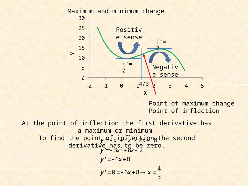
Maximum and minimum change

Point of maximum changePoint of inflection

f’=0

f’=0

Positive sense

Negative sense

At the point of inflection the first derivative has a maximum or minimum.To find the point of inflection the second derivative has to be zero.

34

860''

86''

283'

10242

23

xxy

xy

xxy

xxxy

4/3

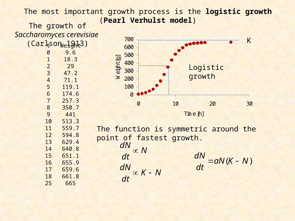
The most important growth process is the logistic growth (Pearl Verhulst model)

t Weight0 9.61 18.32 293 47.24 71.15 119.16 174.67 257.38 350.79 441

10 513.311 559.712 594.813 629.414 640.815 651.116 655.917 659.618 661.825 665

The growth of Saccharomyces cerevisiae (Carlson 1913)

0100200300400500600700

0 10 20 30

Wei

ght [

g]Time [h]

Logistic growth

)( NKaNdtdN

NKdtdN

NdtdN

K

The function is symmetric around the point of fastest growth.

0

5

10

15

20

25

30

0 5 10 15 20

N

t

The most important growth process is the logistic growth (Pearl Verhulst model)

0

0

1 tt

tt

e

KeN

The process converges to an upper limit defined by the carrying capacity K

The population growths fastest at

K/2

2)1( NKr

rNKN

rNdtdN

0

2

4

6

8

10

12

14

0 10 20 30 40 50

Time [h]

Vo

lum

e

Saccharomyces cerevisiae

20

2max2

2 KNN

Kr

rdtNd

N

Maximum population size is at

KNNKr

rNdtdN max

2 0

Differential equation

)5.9(113

te

N

t0

0

0.2

0.4

0.6

0.8

1

1.2

0 20 40 60 80 100

N

t

The change of populations in time

bt

tt

aN

KNN

1

1The Nicholson – Bailey approach to fluctuations of animal populations in time

First order recursive function

K=0.95a=0.05b=2.0

0

500

1000

1500

2000

2500

3000

0 20 40 60 80 100

N

t

K=1. 5a=0.01b=0.5

0.9

0.92

0.94

0.96

0.98

1

1.02

0 20 40 60 80 100

N

t

K=2. 0a=1.2b=3.9

00.20.40.60.8

11.21.41.61.8

0 20 40 60 80 100

N

t

K=3. 0a=3.0b=6.0

A simple deterministic process (function) is able to generate a quasi random (pseudochaotic) pattern.

Hence, seemingly complicated fluctuations of populations in time might be driven by very simple ecological processes

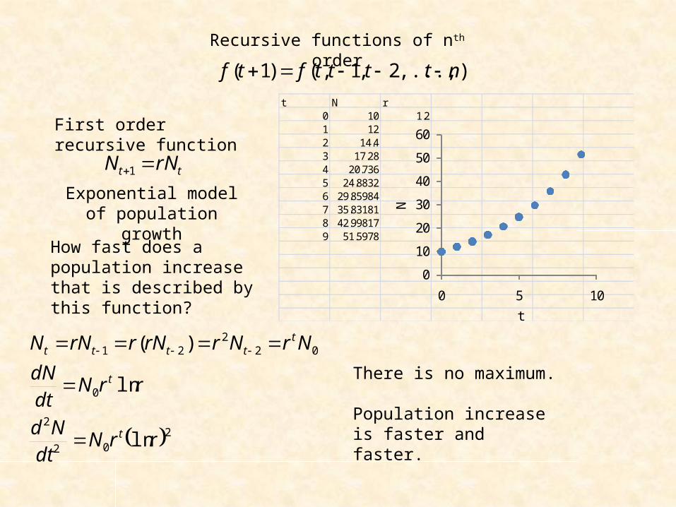
),...,2,1,()1( nttttftf

Recursive functions of nth order

tt rNN 1

First order recursive function

How fast does a population increase that is described by this function?

202

2

0

022

21

ln

ln

)(

rrNdtNd

rrNdtdN

NrNrrNrrNN

t

t

ttttt

There is no maximum.

Population increase is faster and faster.

t N r0 10 1.21 122 14.43 17.284 20.7365 24.88326 29.859847 35.831818 42.998179 51.5978

0

10

20

30

40

50

60

0 5 10

N

t

Exponential model of population growth

bt

tt

aN

KNN

1

1

tbt

ttt N

aN

KNNNN

1

1

Nicholson – Bailey approach

NaNKN

tN

b

1

Difference equation

NaNKN

dtdN

b

1

Differential equation

Where are the maxima of this function?

NaNKN

b

1

0b

b

aK

NaNK1

maxmax

11

The global maximum of the function

0

500

1000

1500

2000

2500

3000

0 20 40 60 80 100

N

t

K=1. 5a=0.01b=0.5

250001.015.1 5.0

1

max

N

Series expansions

)(),(0

xfixgn

i

xxa

axaxaxaxan

n

1)1(

...1

32

Geometric series

We try to expand a function into an arithmetic series. We need the coefficients ai.

......)( 44

33

2210 n

nxaxaxaxaxaaxf

333

433

2222

4322

1113

42

3211

0

32)0(...)1)(2(...43232)(

2)0(...)1(...43322)(

)0(......432)(

)0(

afxnannxaaxf

afxnanxaxaaxf

afxnaxaxaxaaxf

af

nn

nn

nn

i

i

in

n

xif

xnf

xf

xf

xf

xffxf

0

44

33

22

1

!)0(

...!)0(

...!4)0(

!3)0(

!2)0(

)0()0()(

McLaurin series

...)(...)()()()()( 44

33

2210 n

n bxabxabxabxabxaaxf

333

433

2222

4322

1113

42

3211

0

32)(...)()1)(2(...)(43232)(

2)(...)()1(...)(43)(322)(

)(...)(...)(4)(3)(2)(

)(

abfbxnannbxaabf

abfbxnanbxabxaabf

abfbxnabxabxabxaabf

abf

nn

nn

nn

i

i

in

n

bxi

bfbx

n

nfbx

bfbxbfbfxf )(

!

)(...)(

!

)(...)(

!2

)())(()()(

1

22

1

Taylor series

00

04

03

02

000

!1

!...

!...

!4!3!2 i

i

i

nx

ie

ix

xne

xe

xe

xe

xeee

iin

i

nnnnn xanin

xannn

xann

xnaaxa

0

33221

)!1(!!

...!3

)2)(1(!2)1(

)(

Binomial expansion

iin

i

n xai

nxa

0

)( Pascal (binomial) coefficients

i

n

Series expansions are used to numerically compute otherwise intractable functions.

xy sin

i

i

in

n

xif

xnf

xf

xf

xf

xffxf

0

44

33

22

1

!)0(

...!)0(

...!4)0(

!3)0(

!2)0(

)0()0()(

....!7!5!3

...!4)0sin(

!3)0cos(

!2)0sin(

)0cos()0sin()sin(753

432 xxxxxxxxx

Fast convergence

Degrees Radians Sin 1 2 3 4 5 Sum30 0.523599 0.5 0.523599 -0.02392 0.000328 -2.14072E-06 1.55678E-08 0.545 0.785398 0.70711 0.785398 -0.08075 0.00249 -3.65762E-05 3.98984E-07 0.7071160 1.047198 0.86603 1.047198 -0.1914 0.010495 -0.000274012 3.98534E-06 0.8660390 1.570796 1 1.570796 -0.64596 0.079693 -0.004681754 0.00010214 0.99995

Summands

1

15432

)1(...5432

)1ln(i

ii

ixxxxx

xx

Taylor series expansion of logarithms

In the natural sciences and maths angles are always given in radians!

Very slow convergence

Home work and literatureRefresh:

• Arithmetic, geometric series• Limits of functions• Sums of series• Asymptotes• Derivative• Taylor series• Maxima and Minima• Stationary points

Prepare to the next lecture:

• Logistic growth• Lotka Volterra model• Sums of series• Asymptotes

Literature:

Mathe-onlineLogistic growth: http://en.wikipedia.org/wiki/Logistic_functionhttp://www.otherwise.com/population/logistic.html