the demand for local bus services in...

This is a repository copy of The demand for local bus services in England

White Rose Research Online URL for this paperhttpeprintswhiteroseacuk2429

Article

Dargay JM and Hanly M (2002) The demand for local bus services in England Journal of Transport Economics and Policy 36 (1) pp 73-91 ISSN 0022-5258

eprintswhiteroseacukhttpseprintswhiteroseacuk

Reuse

See Attached

Takedown

If you consider content in White Rose Research Online to be in breach of UK law please notify us by emailing eprintswhiteroseacuk including the URL of the record and the reason for the withdrawal request

White Rose Research Online

httpeprintswhiteroseacuk

Institute of Transport StudiesUniversity of Leeds

This is a publisher produced version of a paper from the Journal of Transport Economics and Policy This final version is uploaded with the permission of the publishers The original publication can be found at httpwwwbathacuke-journalsjtep White Rose Repository URL for this paper httpeprintswhiteroseacuk2429

Published paper Dargay JM and Hanly M (2002) The Demand for Local Bus Services in England Journal of Transport Economics and Policy 36(1) pp73-91

White Rose Consortium ePrints Repository eprintswhiteroseacuk

The Demand for Local Bus Services in

England

Joyce M Dargay and Mark Hanly

Address for correspondence Dr Joyce Dargay ESRC Transport Studies Unit Centre for

Transport Studies University College London Gower Street London WC1E 6BT The

authors would like to thank the Department of the Environment Transport and the

Regions of the UK for regnancing this project Steve Grayson the DETR project co-ordi-

nator and the other members of the project team Phil Goodwin (UCL) and Peter Huntley

David Hall and James Rice (TAS Partnership Ltd) for their assistance and advice and the

bus companies which permitted the use of their data They also thank the anonymous

referee and the editor of this Journal for providing helpful suggestions that much improved

the work The views expressed in this paper are solely those of the authors and do not

remacrect those of the DETR or of data contributors

Abstract

This paper examines the demand for local bus services in England The study is based on a

dynamic model relating per capita bus patronage to bus fares income and service level

and is estimated using a combination of time-series and cross-section data for English

counties The results indicate that patronage is relatively fare-sensitive with a wide

variation in the elasticities

Date of receipt of regnal manuscript January 2001

Journal of Transport Economics and Policy Volume 36 Part 1 January 2002 pp73plusmn91

73

Introduction

This paper investigates the demand for local bus services in England It is

based on a project carried out for the Department of the Environment

Transport and the Regions (DETR)1 in the UK The main objective of the

study has been to obtain estimates of fare elasticities that could be used in

policy calculations to project the change in bus patronage nationally as a

result of a given lsquolsquoaveragersquorsquo fare change and to explore possible variation

in the elasticity

Basically two approaches can be used to estimate the fare elasticity

dependent on the type of data utilised The regrst relies on actual data on

bus patronage the second on stated preference surveys Recently there

have been many studies using stated preference methods which when real

data are impossible or dicult to obtain can prove indispensable How-

ever such methods have their limitations and the results are often dicult

to interpret They also require extended ETH and costly ETH data collection

The present analysis is thus entirely based on actual patronage data

In judging the impact of a given change in bus fares it is essential to

deregne the time perspective concerned In recent years two quite diVerent

methods have been used to make such a distinction The regrst is to deregne a

priori certain classes of behavioural response as lsquolsquoshort-termrsquorsquo and others

as lsquolsquolong-termrsquorsquo In principle this enables cross-section models to be

interpreted as indicating something about the time scale of response by

consideration of which responses are included The conditions for this to

be valid are stringent and rarely fulreglled and even where they are no

statements are possible about how many months or years it takes for the

long-term eVect to be completed The second approach is to use time-series

data with a model speciregcation in which a more or less gradual response

over time is explicit the time scale being determined empirically as one of

the key results of the analysis Methodologically this method is far

superior It also has another advantage for policy purposes it is necessary

to know not only the level of the response in the lsquolsquolong runrsquorsquo but also how

long the adjustment takes This can only be achieved on the basis of

dynamic models that explicitly take into account the eVects of fares and

other relevant factors in diVerent time perspectives Such an analysis

requires observations of changes in bus patronage fares and so on over

time The approach taken in this study is to employ a dynamic metho-

dology to investigate the response to fare changes over time

1As a result of a departmental reorganisation in 2001 transport is now part of the

Department of Transport Local Government and the Regions (DTLR)

Journal of Transport Economics and Policy Volume 36 Part 1

74

The estimation of bus fare elasticities is based on annual operatorsrsquo

data for years 1986 to 1996 on bus patronage fares and other relevant

factors inmacruencing bus use which have been obtained from the DETR

The data for the individual operators are aggregated to county level and

combined with information on income and population for the individual

counties

The fare elasticities are estimated on the basis of dynamic econometric

models relating per capita bus patronage (all journeys) to real per capita

income real bus fares (average revenue per journey) service level (bus

vehicle kilometres) real motoring costs and demographic variables The

dynamic methodology employed distinguishes between the short- and

long-term impacts of fare changes on bus patronage as well as providing

an indication of the time required for the total response to be complete

The next section describes the county-level data used for the analysis

The econometric model is presented in the next section followed by sta-

tistical estimates and elasticities The paper ends with some concluding

remarks

Bus Patronage Fares and Service

The data used for the analysis were obtained from the STATS100A

database provided by the DETR This database includes regnancial year

returns to the DETR from bus operators licensed for 20 or more vehicles

It contains information on vehicle miles passenger receipts passengers

carried number of vehicles and staV and (for operators of local services)

concessionary fare contributions public transport support and fuel duty

rebate In addition operators are also asked to estimate a breakdown by

county of passenger journeys and receipts revenue support conces-

sionary fare contributions and vehicle miles as well as information on

operating and administrative expenditure depreciation and proregtability

These data have been collected in this form since the 1986 deregulation of

bus services outside London Permission was sought from the large bus

operators in Great Britain (that is those with a macreet size of 50 or more) to

have access to their returns to the DETR

The data used in this study are for the operators in England who gave

permission to use the information contained in the database These make

up 87 per cent of bus vehicle kilometres and 93 per cent of passenger

journeys in England The operator data was aggregated to the county

level resulting in 46 counties for the regnancial years 198788 to 199697

For simplicity these are referred to as 1987 to 1996

The Demand for Local Bus Services in England Dargay and Hanly

75

The data on bus patronage fares and service for each county were

combined with county level information on population and disposable

income obtained from Regional Statistics

Bus patronage

The data on bus patronage includes all trips both full-fare and conces-

sionary Figure 1 shows average bus journeys per capita for the period 1987

to 1996 on a county level The variation is apparent ranging from over 170

journeys in Tyne and Wear to around 20 in Lincolnshire Of the metro-

politan counties Greater Manchester has the lowest per capita bus use ETH

about half that of Tyne and Wear and London Clearly the metropolitan

areas show the most intensive bus use followed by Nottinghamshire

Durham Lancashire and Leicestershire The majority of counties show an

average bus use of between 20 and 60 journeys per capita In general the

more densely populated counties have a more intensive bus use There are a

number of exceptions however For example the densely populated

counties around London ETH Surrey Berkshire and Hertfordshire ETH have

Figure 1

Bus journeys per capita in English counties Average 1987plusmn96

Tyne amp WearLondon

W MidlandsS Yorkshire

MerseysideW Yorkshire

Gtr ManchesterNottinghamshire

DurhamLancashireLeicestershire

AvonNorthumberland

ClevelandDerbyshireIsle of WightE SussexHumberside

OxfordshireStaffordshire

CheshireDevon

CumbriaHamptonshire

BerkshireBedfordshire

EssexN Yorkshire

NorthamptonshireSuffolkKentBuckinghamshireWorcestershireWiltshireShropshire

GloucestershireHertfordshire

NorfolkDorsetWarwickshire

CambridgeshireSurreySomerset

CornwallW SussexLincolnshire

0 20 40 60 80 100 120 140 160 180 200

Mean journeys per capita


76

relatively low bus use while sparsely populated Northumberland has a

comparatively high per capita patronage

As is the case for Great Britain as a whole bus use has been declining over

the past decade in most English counties During the period 1986plusmn1996

the average decline was approximately 20 per cent Only Oxfordshire has

shown a continual increase in patronage

Bus fare

Since the STATS100A database provides no information on fares these

have to be calculated on the basis of data on revenues and journeys There

are two alternatives passenger receipts including or excluding conces-

sionary fare reimbursement (CFR) By including CFR we obtain an

approximate measure of the average non-concessionary fare that is fare

without concessions Excluding the CFR gives a measure of the average

fare actually paid by all bus patrons Since the patronage data include

concessions as well as full-fare-paying patrons this latter fare deregnition is

the more appropriate and it allows for a changing mix of passenger

categories The fare variable is thus calculated as real average revenue per

passenger journey excluding concessionary fare reimbursement

The average fares calculated in this manner for each of the counties

over the period are shown in Figure 2 The considerable variation amongst

Figure 2

Bus fares in English counties 1995 pound per journey Average 1987plusmn96

CambridgeshireIsle of Wight

SurreyKentBedfordshire

HertfordshireEssex

BuckinghamshireCornwallE Sussex

W SussexWarwickshire

NorfolkDorset

SomersetNorthumberland

WiltshireDevon

AvonOxfordshire

BerkshireDerbyshire

NorthamptonshireGloucestershire

LeicestershireN Yorkshire

CumbriaHumberside

HamptonshireLincolnshireLancashire

StaffordshireDurham

ShropshireSuffolk

NottinghamshireWorcestershire

CheshireGtr Manchester

W YorkshireS YorkshireLondon

ClevelandW Midlands

Tyne amp WearMerseyside

0 01 02 03 04 05 06 07 08 09 1

Average revenue per journey 1995 pound


77

counties is apparent ETH from 22 pence per journey in Merseyside to 88

pence in Cambridgeshire Fares are on average considerably lower in the

more urban counties ETH London the six former Metropolitan counties of

England and Cleveland than in the more suburban and rural counties

In general the counties with the lowest fares have the most favourable

concessionary schemes The counties with the lowest fares ETH London the

Metropolitan counties and Cleveland ETH have a very high proportion of

CFR while those with the highest fares ETH Cambridgeshire Surrey Isle of

Wight Kent and Bedfordshire ETH have a low proportion of CFR There

are a few obvious exceptions Cheshire for example has a relatively low

fare but also a low proportion of CFR There is substantial variation in

the proportion of concessionary fare reimbursement across counties from

40 per cent in Merseyside to 0 per cent in Bedfordshire In the majority of

counties CFR is well under 20 per cent of total receipts The only

exceptions are the former Metropolitan counties and Cleveland and

SuVolk

In real terms average revenue has gone up in most English counties

since deregulation in 1986 In about 10 per cent of counties the increase

was over 40 per cent On average the increase was about 20 per cent The

greatest fare increases are noted for Cleveland and South Yorkshire In a

few counties ETH Cumbria Norfolk and West Midlands ETH fares have

remained more or less constant over the period and only in one county

(Oxfordshire) have fares actually fallen

Figure 3

Relationship between average fares and bus patronage in English counties 1987plusmn96

0

20

40

60

80

100

120

140

160

180

200

0 01 02 03 04 05 06 07 08 09 1

Average fare 1988-96 1995 pound

Ave

rag

e jo

urn

eys p

er

ca

pita 1

988

-96 Tyne amp Wear

London


ClevelandIsle of Wight

Cambridgeshire

Lincolnshire

Cheshire

WorchestershireSuffolk

Shropshire


78

The relationship between average fares and journeys per capita is illu-

strated in Figure 3 There does appear to be a negative relationship ETH

although not a linear one ETH between patronage and fare level A number

of counties however show a signiregcant deviation from the lsquolsquobest-regtrsquorsquo line

Particularly patronage is higher in Tyne amp Wear London and the Isle of

Wight than would be suggested by their fare levels Similarly patronage is

lower in Cleveland Cheshire Worcestershire Lincolnshire SuVolk and

Shropshire

Service

Bus vehicle kilometres per capita is used as the proxy for level of service

The large variation among the counties is illustrated in Figure 4 Tyne amp

Wear has the highest service intensity and West Sussex the lowest In

general the most densely populated counties have better bus service than

more rural counties Overall bus vehicle kilometres tend to be higher in

the six former Metropolitan counties of England than elsewhere in the

country Again this is not very surprising

In most counties bus service has been increasing over the past 10 years

The greatest percentage increases are in Cleveland Surrey Oxfordshire

Gloucestershire and Bedfordshire ETH well over 40 per cent in all cases

Figure 4

Bus kilometres per capita in English counties Average 1987-96

Tyne amp WearS Yorkshire


DurhamGtr Manchester

NorthumberlandW Midlands

LondonAvon

NottinghamshireDevon

LancashireLeicestershire

Isle of WightDerbyshire


BuckinghamshireHamptonshireCheshire

E SussexCumbriaHumberside

EssexBedfordshire

ClevelandN Yorkshire

WorcestershireShropshire

HertfordshireKent

WiltshireCambridgeshireSuffolkNorfolkWarwickshireNorthamptonshire

CornwallSomerset

BerkshireDorsetGloucestershireSurrey

LincolnshireW Sussex

0 10 20 30 40 50 60 70 80 90

Bus kilometres per capita


79

Buckinghamshire Hertfordshire and Derbyshire show the greatest decline

For most other counties service has increased by less than 20 per cent

The Model

Because of the aggregate nature of the available data a relatively simple

model is used to model bus patronage We assume that the long-run

equilibrium demand for bus services in terms of journeys per capita QcurrenRt

in county R in year t can be expressed as a function f of the bus fare FRt

the service level SRt per capita disposable income IRt demographic

factors DRt (population density the percentage of pensioners in the

population) and the cost of alternative modes For the latter we assume

that the only viable substitute for bus travel is car use so the cost of

alternative modes is represented by motoring costs However as these are

not available on a county level national data2

are used so that motoring

costs Mt vary over time but are assumed to be the same for all counties3

QcurrenRt ˆ f FRt SRt IRt Mt DRt

iexcl cent

hellip1dagger

In estimating the demand model we assume that all explanatory variables

are given or determined exogenously Although the service variable (bus

kilometres per capita) can also be seen as a measure of supply which itself

is determined by demand we assume that supply in any given year is

unaVected by demand changes within the same year This may be a strong

assumption and it would be preferable to estimate the complete supplyplusmn

demand system

In order to account for lags in the adjustment to changes in the

explanatory variables a partial adjustment model4

is used to relate actual

patronage QRt to its long-run equilibrium level This results in the fol-

lowing model

QRt ˆ f FRt SRt IRt Mt DRthellip dagger Dagger yRQRtiexcl1 hellip2dagger

where 0 micro yR lt 1 The adjustment coecient 1 iexcl yR indicates the pro-

portion of the gap between equilibrium and actual patronage that is closed

each year The presence of demand in the previous period on the right-

2The index of total motoring costs obtained from the DETR includes all running costs as

well as car purchase costs3Although there may be some diVerences in the cost of motoring among counties it is not

unreasonable to assume that development over time is similar4Dargay and Hanly (1999) use both partial adjustment and error-correction models for

aggregate GB data However the time period available for the county data is too short to

apply cointegration tests


80

hand side of the equation can be interpreted in terms of habits or inertia ETH

what individuals do in the past also aVects their future behaviour Also

since demand in period t iexcl 1 is inmacruenced by prices and so on in period

t iexcl 1 and similarly for all other previous periods demand in any period is

determined by the entire past history of prices and other relevant vari-

ables Individuals do not respond to changing circumstances instanta-

neously but with a delay

Assuming f to be a linear function and all variables to be in logarithmic

forms results in the following constant elasticity speciregcation

LnQRt ˆ aR Dagger bFRLnFRt Dagger bSRLnSRt Dagger bIRLnIRt

Dagger bMLnMt Dagger bDRLnDRt Dagger yRLnQRtiexcl1 hellip3dagger

The short-run elasticities are obtained directly from the coecients of the

independent variables while the long-run elasticities are calculated as the

short-run elasticities divided by the adjustment coecient hellip1 iexcl ydaggerR The

greater the value of yR the slower the speed of adjustment and the greater

the diVerence between the short- and long-run elasticities

In the speciregcation shown above the elasticities are constant and

independent of the levels of the independent variables An alternative

speciregcation which allows the fare elasticity to be related to the fare level

can be written as

LnQRt ˆ aR Dagger bFRFRt Dagger bSRLnSRt Dagger bIRLnIRt

Dagger bMnMt Dagger bDRnDRt Dagger yLnQRtiexcl1 hellip4dagger

Here the short-run fare elasticity is equal to bFRFRt and the long-run

elasticity equal to bFRFRt=hellip1 iexcl yRdagger so that both elasticities vary over time

and increase with the fare level Since this model has the same dependent

variable as the constant elasticity model the choice between them can be

made on the basis of simple statistical tests

Equations (3) and (4) can be estimated separately for each county so

that county-speciregc fare income and service elasticities can be obtained

However given the short time period for which we have data ETH 10 annual

observations ETH such an approach would not provide reliable estimates of

the model parameters For this reason the model is estimated by pooling

the time-series data for the individual counties By combining the data in

the estimation procedure the number of observations (and degrees of

freedom) is increased thus improving the signiregcance of the estimated

parameters It also provides more variation in the data since patronage

and fares vary more between counties than over time The disadvantage of

this technique however is that it assumes that the demand relationship

and the elasticities are the same for all counties In pooling diVerences


81

between regions that are not captured in the included explanatory vari-

ables can be assumed to be either regxed or random In the Fixed EVects

Model diVerences between counties can be represented by county-speciregc

intercepts hellipaRdagger The Random EVects Model on the other hand represents

the diVerences between regions as diVerences in the random error term

There is no a priori manner of choosing which speciregcation is the more

appropriate and the choice must be based on statistical tests The fol-

lowing discussion is based on a Fixed EVects Model although both Fixed

and Random EVects speciregcations were estimated5

In the empirical work we estimate two forms of the pooled model In

the most restricted form it is assumed that all slope coecients (the bs and

ydagger are the same for all counties and that diVerences between counties can

be represented by county-speciregc intercepts hellipaRdagger

LnQRt ˆ aR Dagger bFLnFRt Dagger bSLnSRt Dagger bILnIRt

Dagger bMLnM Dagger bDLnDRt Dagger yLnQRtiexcl1 hellip5dagger

For the constant elasticity model above the elasticities are the same for all

counties For the variable fare elasticity model in (4) the fare elasticity is

dependent on the fare level so that it will vary amongst counties inversely

in relation to their fares

The second model also allows the coecient of the fare variable (or the

fare elasticity in the constant elasticity model) to be region speciregc

LnQRt ˆ aR Dagger bFRLnFRt Dagger bSLnSRt Dagger bILnIRt

Dagger bMLnMt Dagger bDLnDRt Dagger yLnQRtiexcl1 hellip6dagger

where bFR is the coecient relating to the fare variable for county R aR is

the county-speciregc intercept term and all other coecients are con-

strained to be equal for all counties For the constant elasticity model

above the fare elasticity can vary among counties but will be the same for

each county over time and for all fare levels For the variable elasticity

model the fare elasticity will vary both among counties as well as over

time for each county dependent on the fare level Model (5) is a restricted

form of model (6) that is with bFR ˆ bF for all counties This can be

tested using a simple statistical test

5Using a Hausman Test to test between the Fixed and Random EVects speciregcations

results in test statistics of 299 and 307 for the constant and variable elasticity model

respectively clearly rejecting the Random EVects speciregcation in preference to the Fixed

EVects


82

Model Estimation

The four variants of the model described in the previous section were

estimated from the combined time-series cross-section data for English

counties The natural logarithm of bus journeys per capita is the dependent

variable for all the estimations The fare and service variables are as

described in the previous section Income is deregned as household dis-

posable income per capita motoring costs as the national index and all

price and income variables are converted to 1995 prices using the Retail

Price Index Initially two demographic variables were included popula-

tion density and the percentage of pensioners in the county6 However as

population density was not found to be signiregcant in any of the specireg-

cations the models presented below exclude this variable7

Since a lagged dependent variable is included among the regressors the

regrst observation is lost for each county so that we have nine annual

observations for each of the 46 counties a total of 414 observations

Two speciregcations are estimated ETH one constraining all coecients to

be the same across counties and one in which the coecients of the fare

variable and thus the price elasticity are county-speciregc In addition for

each of the speciregcations (constrained and unconstrained) two diVerent

functional speciregcations are estimated (a) a lsquolsquoconstant elasticityrsquorsquo model in

which all variables are specireged in natural logarithms and whose coe-

cients yield the elasticities of interest directly and (b) a model in which all

variables are in natural logarithms except the price (fare) variable which is

specireged in level terms In the latter the elasticity is not constant but

increases with the price level (bus fare)

The estimated parameters (with the exception of the county-speciregc

intercept terms) for the constrained models are reported in Table 1 and for

the unconstrained model in Table 2 In all cases the models regt the data

well with adjusted R-squared values very near one and the F-tests for the

regxed eVects conregrming the importance of individual intercepts The esti-

mated coecients are generally of the expected signs ETH income and the

bus fare have negative eVects on bus patronage whereas service motoring

costs and the percentage of pensioners have a positive inmacruence The

coecients of income service motoring costs the percentage of pen-

sioners and the lagged patronage variable are nearly identical in both

constrained models as they are in both unconstrained models However

6Income population and the number of pensioners on a county level were obtained from

Regional Statistics7As population density varies little over time its eVects are captured in the county-speciregc

intercept terms


83

comparing the constrained models with the unconstrained we see that the

coecients of income motoring costs and percentage of pensioners are

greater in absolute value in the unconstrained models Adjustment appears

to be quicker in the unconstrained model with 58 per cent of total

adjustment occurring within one year as opposed to 48 per cent in the

constrained models All estimated coecients with the exception of the

percentage of pensioners are highly signiregcant in the constrained models

(Table 1) while the fare coecients are signiregcant for slightly less than

half the 46 counties in the unconstrained model (Table 2) The poor sig-

niregcance of the fare coecients in the unconstrained model (only 21 of the

46 fare coecients are signiregcant at the 5 level) is a result of the small

number of observations on which the county-speciregc estimates are based

Table 1Constrained Model Estimates

Dependent variable Journeys per capita 414 observations

Constant Fare Elasticity Variable Fare Elasticity

Variable Coecient T-Statistic Coecient T-Statistic

Journeys(-1) 052 1010 052 1033

Income iexcl039 iexcl314 iexcl039 iexcl324

Service 049 599 047 595

Motoring Costs 032 387 035 433

Percent Pensioners iexcl008 iexcl054 iexcl001 iexcl010

Fare iexcl033 iexcl487 iexcl074 iexcl679

Adjusted R-squared 09998 09998

SSE 19113 18246

Log Likelihood 5258225 5354312

F-test Fixed EVects 426 hellipP ˆ 0000dagger 470 hellipP ˆ 0000dagger

Note coecients in bold type are signiregcant at the 95 level

The statistical tests for model selection are shown in Table 3 The regrst set

of tests shown concern the functional relationship between patronage and

fares that is the constant versus the variable elasticity formulations8 For

both the model with common fare coecients (constrained) and the model

with county-speciregc fare coecients (unconstrained) the variable elasti-

city (semi-log) speciregcation is the one preferred The fare elasticity is thus

not constant but depends on the fare level In the second set of tests the

hypothesis of common fare coecients is tested against county-speciregc

fare coecients9 For both the constant and variable elasticity models the

8Based on a Likelihood Ratio Test of the Likelihood values of the respective models9Based on an F-test comparing the SSE of the restricted and unrestricted models


84

Table 2Unconstrained Model Estimates County Speciregc Fare Elasticity


Constant fare elasticity Variable fare elasticityVariable Coecient T-Statistic Coecient T-Statistic

Journeys(-1) 042 663 042 663Income iexcl057 iexcl416 iexcl060 iexcl440Service 048 519 049 525Motoring Costs 065 717 065 741

Percent Pensioners 044 264 049 291Fare Northumberland iexcl006 iexcl002 iexcl009 iexcl002Cumbria iexcl055 iexcl080 iexcl108 iexcl078

Durham 004 007 005 004Tyne amp Wear iexcl045 iexcl439 iexcl154 iexcl479Cleveland 006 026 015 018

North Yorkshire iexcl024 iexcl038 iexcl044 iexcl035Lancashire 000 001 002 004West Yorkshire iexcl039 iexcl417 iexcl104 iexcl390Humberside iexcl121 iexcl1095 iexcl208 iexcl1332

South Yorkshire iexcl067 iexcl590 iexcl194 iexcl557Merseyside 021 103 081 098Manchester iexcl052 iexcl537 iexcl115 iexcl525Cheshire iexcl038 iexcl065 iexcl090 iexcl075

Derbyshire iexcl034 iexcl156 iexcl057 iexcl155Nottinghamshire iexcl043 iexcl299 iexcl092 iexcl300Lincolnshire iexcl022 iexcl034 iexcl053 iexcl040

StaVordshire iexcl064 iexcl143 iexcl123 iexcl143Shropshire iexcl001 iexcl002 002 002Leicestershire iexcl048 iexcl270 iexcl089 iexcl277Norfolk iexcl164 iexcl340 iexcl254 iexcl359

West Midlands iexcl154 iexcl902 iexcl498 iexcl904Worcestershire iexcl071 iexcl217 iexcl162 iexcl224Warwickshire iexcl016 iexcl046 iexcl022 iexcl044Northamptonshire iexcl044 iexcl121 iexcl079 iexcl125

Cambridgeshire iexcl100 iexcl354 iexcl113 iexcl358SuVolk iexcl030 iexcl079 iexcl065 iexcl081

Gloucestershire iexcl001 iexcl001 iexcl003 iexcl002Oxfordshire iexcl049 iexcl272 iexcl092 iexcl340Buckinghamshire iexcl031 iexcl075 iexcl043 iexcl078Bedfordshire iexcl053 iexcl120 iexcl070 iexcl127

Hertfordshire iexcl050 iexcl220 iexcl067 iexcl190Essex iexcl013 iexcl053 iexcl019 iexcl054Avon iexcl069 iexcl293 iexcl111 iexcl283Wiltshire iexcl030 iexcl054 iexcl045 iexcl050

Berkshire iexcl049 iexcl237 iexcl085 iexcl263London 028 369 104 419Cornwall iexcl051 iexcl128 iexcl077 iexcl127

Devon iexcl091 iexcl189 iexcl155 iexcl197Somerset 148 050 240 052Dorset iexcl019 iexcl031 iexcl034 iexcl035Hampshire iexcl079 iexcl557 iexcl147 iexcl570

Surrey iexcl115 iexcl317 iexcl149 iexcl333Kent iexcl068 iexcl442 iexcl086 iexcl453West Sussex iexcl032 iexcl026 iexcl053 iexcl029East Sussex iexcl080 iexcl294 iexcl119 iexcl290

Isle of Wight iexcl066 iexcl080 iexcl076 iexcl076Adjusted R-squared 09998 09998SEE 14311 14143

Log Likelihood 5857099 5881617F-test Fixed EVects 257 hellipP ˆ 0000dagger 307 hellipP ˆ 0000dagger



85

constrained versions are rejected in favour of the unconstrained for-

mulations implying that the fare elasticity is not the same for all counties

In summary the statistical tests favour the unconstrained variable elasti-

city model implying that fare elasticity both varies among counties and

increases with the level of fare This implies that the variation in fare

elasticities among counties is not solely explained by diVerences in fares10

The resulting elasticities for the four model speciregcations are shown in

Table 4 The regrst two rows report the elasticities for the constrained and

unconstrained versions of the constant elasticity model The fare elasticity

shown for the unconstrained model is the average of the elasticities esti-

mated for the individual counties The next set of results is for the variable

Table 3Tests for Various Model Formulations

Test Probability Conclusion

Tests for variable versusconstant elasticityCommon fare coecients Agrave2 ˆ 192 Prob ˆ 000 Reject constant elasticity modelCounty-speciregc fare coecients Agrave2 ˆ 490 Prob ˆ 003 Reject constant elasticity model

Tests for common fare SSEcoecientsConstant elasticity model F ˆ 236 Prob ˆ 000 Reject common fare coecientsVariable elasticity model F ˆ 204 Prob ˆ 000 Reject common fare coecients

Table 4Estimated Short-run (SR) and Long-run (LR) Elasticities Based on Pooled

Data for English Counties

Fare Income Service Motoring

Costs Pensioners

SR LR SR LR SR LR SR LR SR LRConstant elasticity

Constrained iexcl033 iexcl068 iexcl039 iexcl082 049 103 032 066 hellipiexcl008dagger hellipiexcl017daggerUnconstrained iexcl043 iexcl074 iexcl057 iexcl098 048 083 065 112 044 075

Variable elasticityConstrained iexcl039 iexcl081 049 083 035 072 hellipiexcl001dagger hellipiexcl003daggerMinimum fare ˆ 17p iexcl013 iexcl026Average fare ˆ 56p iexcl041 iexcl086Maximum fare ˆ pound1 iexcl074 iexcl153

Unconstrained iexcl060 iexcl102 042 079 065 112 049 085Minimum fare ˆ 17p iexcl013 iexcl023Average fare ˆ 56p iexcl044 iexcl075Maximum fare ˆ pound1 iexcl079 iexcl135

Aggregate GB iexcl033 iexcl062 041 iexcl080 Not estimated

average of individual elasticities for all counties () elasticities not signiregcantly diVerent from zero

10 This is a slightly diVerent result from that obtained in Dargay and Hanly (1999) using a

speciregcation which excluded motoring costs and the percentage of pensioners


86

elasticity model In the constrained model the fare elasticity is dependent

on the fare level and the fare elasticities shown in the table are calculated at

the minimum average and maximum fare (in 1995 pound) for all counties over

the observation period For the unconstrained model the fare elasticity

varies by county as well as by fare level The elasticities shown are the

averages of the elasticities for the individual counties calculated at the same

minimum average and maximum fares The lsquolsquoaverage farersquorsquo elasticities are

very similar in both speciregcations and they are also close to the average

elasticity in the unconstrained constant elasticity model For the other

variables the major diVerences in the elasticities occur between the con-

strained and unconstrained versions The income elasticity is slightly more

negative in the unconstrained models the service elasticity slightly smaller

and the impact of motoring costs and the percentage of pensioners greater

As the statistical tests favour the unconstrained variable elasticity model

the elasticities resulting from this speciregcation are those preferred

For comparison the elasticities obtained in Dargay and Hanly (1999)

from the aggregate GB data using the same fare variable are shown in the

table We would expect the results to be roughly similar However we

would not expect the results to be perfectly identical since the present dataset is slightly less inclusive than that used for the aggregate models leaving

out as it does those operators with a macreet size of less than regfty vehicles

which account for approximately 15 per cent of national passenger receipts

Also the aggregate GB estimates are based on a much longer observation

period Despite this the resulting elasticities are not very diVerent

The unconstrained models allow us to calculate separate fare elasticities

for each county These range from 0 (not statistically diVerent from 0) toiexcl16 in the short run and iexcl30 in the long run Clearly these elasticities

must be interpreted with caution based as they are on so few data

observations At best they give an indication of the wide range in which

the fare elasticity can fall in speciregc areas

The variable fare elasticity model also results in diVerent elasticities for

individual counties As shown in Figure 2 above the mean fare over the

period for the individual counties ranges from 25 pence per journey in

Merseyside to nearly 90 pence in Cambridgeshire For the variable elas-

ticity model the average elasticities for the individual counties will show a

similar range of variation The long-run elasticities for the individual

counties calculated at the mean fare in each county over the 1987plusmn1996

period range from iexcl04 in Merseyside to iexcl14 in Cambridgeshire with

the majority of counties lying in the region of iexcl07 to iexcl11

In order further to investigate diVerences in fare elasticities between

urban and less urban areas separate models were estimated for the Shire

counties and the Metropolitan areas These are reported in Table 5 and


87

the resulting elasticities presented in Table 6 Both the fare and service

elasticities are higher in the Shire counties than in the Metropolitan areas

while the opposite is the case for the elasticity with respect to motoring

costs These results are not unreasonable Bus fares and service provision

will have more of an eVect in rural areas than in urban areas because car

use is less advantageous in urban areas given congestion parking and so

on Motoring costs have less of an eVect on bus patronage in rural areas

because bus use is a less viable alternative for many car trips than it is in

urban areas with better bus services Finally income has a greater negative

eVect on bus use in urban areas This is contrary to expectations given the

relative advantage of motoring in rural areas but may remacrect the fact that

Table 5Model Estimates Constant Elasticity Model Common Fare ElasticityEnglish Shire Counties and Metropolitan Counties (excluding London)

Estimated Separately

Dependent variable Journeys per capita

Shire counties Metropolitan counties

39 counties 6 counties

351 observations 54 observations


Journeys(-1) 026 529 051 577


Service 072 1143 036 389

Motoring Costs iexcl017 iexcl085 034 181

Percent Pensioners 073 196 iexcl115 iexcl220


Mean Fixed EVect 248 141 1361 498


SSE 19881 00372



Table 6Estimated Short-Run (SR) and Long-Run (LR) Elasticities for English

Shire Counties and Metropolitan Areas

Fare Income Service Motoring Costs

SR LR SR LR SR LR SR LR

Metropolitan areas iexcl026 iexcl054 iexcl126 iexcl258 036 073 034 069

Shire counties iexcl049 iexcl066 iexcl043 iexcl058 072 097 hellipiexcl017dagger hellipiexcl023dagger

Note Elasticities in parenthesis are not signiregcantly diVerent from zero


88

car ownership is closer to saturation in rural areas so that increasing

income has a greater eVect on car ownership and thus a greater negative

impact on bus use in urban areas

Conclusions

The econometric results presented above suggest that the most likely values

of the fare elasticity for England as a whole are around iexcl04 in the short run

and iexcl09 in the long run The evidence suggests that the long-run elasticities

are about twice the short-run elasticities

Models with separate fare elasticities for each county are statistically

preferred to speciregcations in which the fare elasticity is constrained to be

equal for all counties The results of the unconstrained models show a

considerable variation in the fare elasticity across counties ETH a range from

0 to over iexcl30 in the long run

There is statistical evidence that demand is more price-sensitive at

higher fare levels This conclusion is drawn on the basis of models in which

the fare elasticity is related to the fare level The variation in the elasticity

ranges from iexcl01 in the short run and iexcl02 in the long run for the lowest

fares (17 pence in 1995 prices) to iexcl08 in the short run and iexcl14 in the long

run for the highest fares (pound1 in 1995 prices)

Separate estimates of the fare elasticity for the Shire counties and the

Metropolitan areas (excluding London) indicate that patronage in the

former is on average more sensitive to fare changes than in the latter and

signiregcantly so The less-elastic demand in the Metropolitan areas can be

explained in terms of their urban characteristics better bus service pro-

vision and lower fares

The measure of service quality used in this study is per capita bus

kilometres for the market considered Clearly this is a very crude

approximation for the many factors that make up the quality of a bus

service It is however the only feasible measure on the aggregate level

and the one most commonly used in such studies In general the estimated

service elasticities are the same order of magnitude as or slightly larger

than the fare elasticities although opposite in sign This suggests that an

increase in fares combined with an increase in service would leave demand

unchanged For example if fares were increased by 10 per cent and the

number of vehicle kilometres also increased by 10 per cent patronage

would remain approximately the same as previously

All the evidence is in agreement regarding the sign of the income

elasticity ETH it is negative in the long run suggesting bus travel to be an


89

inferior good This is in agreement with most other studies11 The negative

long-run elasticity remacrects the eVect of income through its positive eVect on

car ownership and use and the negative eVect of the latter on bus

patronage It should be stressed however that the negative income elas-

ticity pertains to a period of rising car ownership and use As private

motoring approaches saturation which it must do eventually or is limited

by political means it is likely that incomersquos negative eVect on bus

patronage will become smaller and possibly become positive

Motoring costs are shown to have a signiregcant positive inmacruence on

bus use particularly in urban areas Of the demographic variables inclu-

ded in the model ETH population density and the percentage of pensioners

ETH only the latter is found to have a signiregcant inmacruence on bus patronage

The non-signiregcance of population density is most probably explained by

the fact that diVerences in population density between counties are cap-

tured by the county-speciregc regxed eVects

It is our general assessment that the average fare elasticities obtained

and the relationship between short- and long-term eVects are quite robust

results adequately supported by the quality of the data available and the

statistical tests The results for the individual counties are less well sup-

ported and at least some of the diVerences noted are likely to be due to

inadequate data rather than remacrecting genuine diVerences

The values for the fare income and service elasticity variables obtained

from the dynamic models in this study are broadly in line with those cited

in the literature The review in Dargay and Hanly (1999) which is based

on those in Goodwin (1992) and Oum Walters and Yong (1992) as well

as more recent studies suggests a consensus value for the short-run elas-

ticity on the order of iexcl03 There is also a good deal of empirical evidence

that the elasticity increases over time with the long-run elasticities gen-

erally from 15 to over 3 times higher than the short-run elasticities

Although there is far less agreement as to the long-run elasticity the

majority of estimates range from iexcl05 to iexcl10 A most striking feature of

the reviews is the variation in the elasticities obtained in the individual

studies which is not surprising given the diVerences in data and metho-

dology used and circumstances considered The studies indicate that the

fare elasticity varies by trip purpose time of day and type of patron The

11 Romilly (2001) regnds the income elasticity based on aggregate data for Great Britain to be

positive This appears to be due to the inclusion of a time trend amongst the explanatory

variables rather than to diVerences in model speciregcation or methodology Compare

Dargay and Hanly (2002) using a cointegration approach on aggregate data Introducing

a time trend into the models estimated here shows that the time trend has a signiregcant

negative eVect and changes the income elasticity from negative to positive We do not

include a time trend here because it has no economic justiregcation


90

elasticity for leisure and other oV-peak trips is about twice that for com-

muting peak-time trips Higher income groups seem to be more sensitive

to changes in bus fares and non-concessionary patrons more responsive

than concessionary patrons

References

Dargay J M and M Hanly (1999) lsquolsquoBus Fare Elasticities Report to the Department of

the Environment Transport and the Regionsrsquorsquo ESRC TSU December

Dargay J M and M Hanly (2002) lsquolsquoBus Patronage in Great Britain an Economic

Analysisrsquorsquo Transportation Research Record forthcoming

Goodwin PB (1992) lsquolsquoA Review of New Demand Elasticities with Special Reference to

Short and Long Run EVects of Price Chargesrsquorsquo Journal of Transport Economics and

Policy 26 155-70

Romilly P (2001) Subsidy and local bus service deregulation in Britain a re-evaluation

Journal of Transport Economics and Policy 35

Oum TH WG Waters II and JS Yong (1992) lsquolsquoConcepts of Price Elasticities of

Transport Demand and Recent Empirical Estimatesrsquorsquo Journal of Transport Economics

and Policy 26 139plusmn54


91

demand for bus services coverpdf

The demand for local bus services in Englandpdf

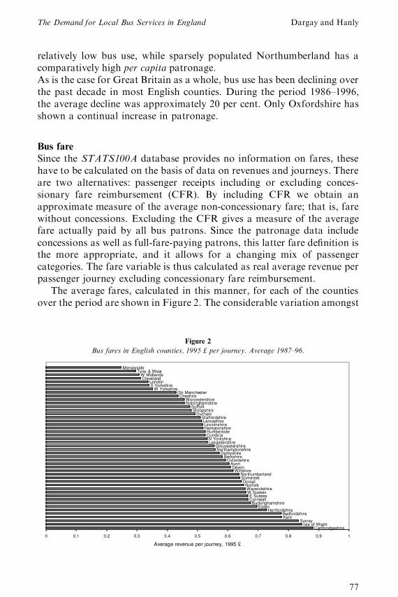
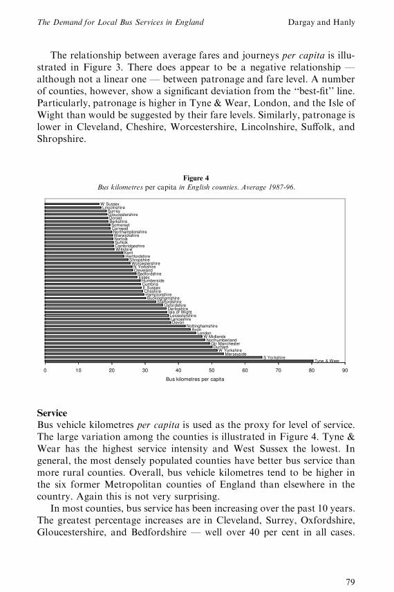
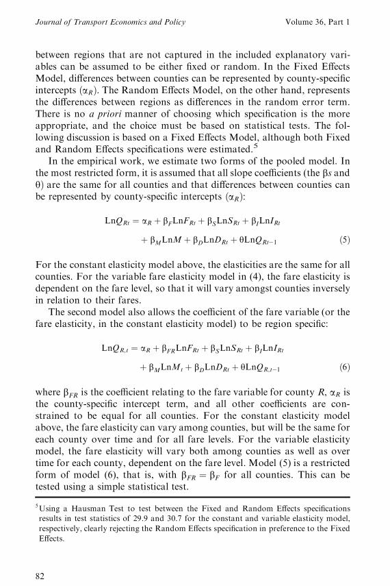
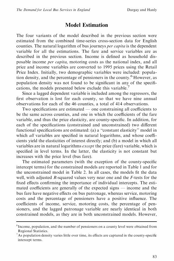
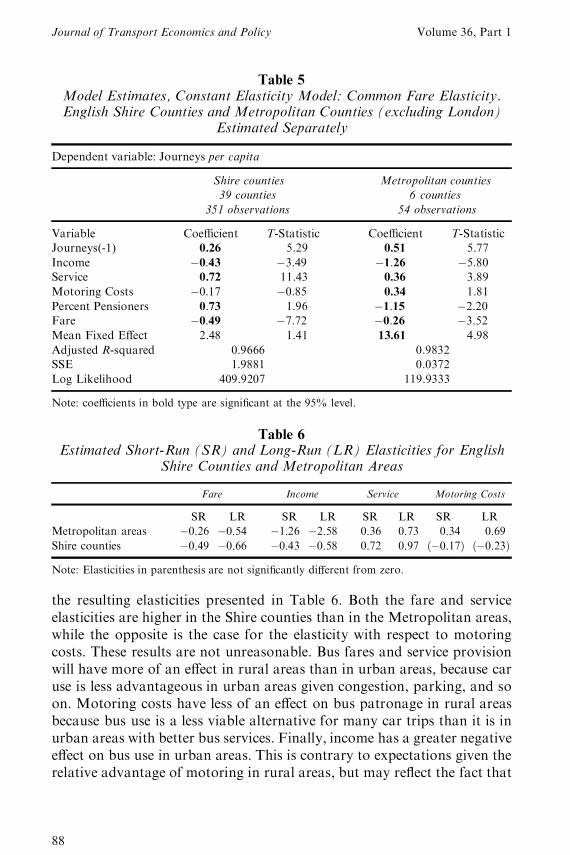White Rose Research Online

httpeprintswhiteroseacuk

Institute of Transport StudiesUniversity of Leeds

This is a publisher produced version of a paper from the Journal of Transport Economics and Policy This final version is uploaded with the permission of the publishers The original publication can be found at httpwwwbathacuke-journalsjtep White Rose Repository URL for this paper httpeprintswhiteroseacuk2429

Published paper Dargay JM and Hanly M (2002) The Demand for Local Bus Services in England Journal of Transport Economics and Policy 36(1) pp73-91

White Rose Consortium ePrints Repository eprintswhiteroseacuk


England












Abstract








73

Introduction







in the elasticity

































74






counties











remarks























75




Bus patronage













Figure 1


Tyne amp WearLondon





AvonNorthumberland



CheshireDevon

CumbriaHamptonshire


EssexN Yorkshire






0 20 40 60 80 100 120 140 160 180 200



76







Bus fare














Figure 2




HertfordshireEssex



NorfolkDorset


WiltshireDevon

AvonOxfordshire

BerkshireDerbyshire



CumbriaHumberside


StaffordshireDurham

ShropshireSuffolk




ClevelandW Midlands


0 01 02 03 04 05 06 07 08 09 1



77
















SuVolk








Figure 3


0

20

40

60

80

100

120

140

160

180

200

0 01 02 03 04 05 06 07 08 09 1


Ave

rag

e jo

urn

eys p

er

ca

pita 1

988

-96 Tyne amp Wear

London



Cambridgeshire

Lincolnshire

Cheshire


Shropshire


78








Shropshire

Service











Figure 4






LondonAvon







EssexBedfordshire



HertfordshireKent


CornwallSomerset



0 10 20 30 40 50 60 70 80 90



79



The Model














iexcl cent

hellip1dagger







demand system





lowing model











80




















can be written as





















81




































EVects


82

Model Estimation






































intercept terms


83

















Journeys(-1) 052 1010 052 1033


Service 049 599 047 595





SSE 19113 18246















84






















85



















Costs Pensioners










86










































87



















Journeys(-1) 026 529 051 577


Service 072 1143 036 389






SSE 19881 00372











88




Conclusions




































89












































90





References







Policy 26 155-70







91




England












Abstract








73

Introduction







in the elasticity

































74






counties











remarks























75




Bus patronage













Figure 1


Tyne amp WearLondon





AvonNorthumberland



CheshireDevon

CumbriaHamptonshire


EssexN Yorkshire






0 20 40 60 80 100 120 140 160 180 200



76







Bus fare














Figure 2




HertfordshireEssex



NorfolkDorset


WiltshireDevon

AvonOxfordshire

BerkshireDerbyshire



CumbriaHumberside


StaffordshireDurham

ShropshireSuffolk




ClevelandW Midlands


0 01 02 03 04 05 06 07 08 09 1



77
















SuVolk








Figure 3


0

20

40

60

80

100

120

140

160

180

200

0 01 02 03 04 05 06 07 08 09 1


Ave

rag

e jo

urn

eys p

er

ca

pita 1

988

-96 Tyne amp Wear

London



Cambridgeshire

Lincolnshire

Cheshire


Shropshire


78








Shropshire

Service











Figure 4






LondonAvon







EssexBedfordshire



HertfordshireKent


CornwallSomerset



0 10 20 30 40 50 60 70 80 90



79



The Model














iexcl cent

hellip1dagger







demand system





lowing model











80




















can be written as





















81




































EVects


82

Model Estimation






































intercept terms


83

















Journeys(-1) 052 1010 052 1033


Service 049 599 047 595





SSE 19113 18246















84






















85



















Costs Pensioners










86










































87



















Journeys(-1) 026 529 051 577


Service 072 1143 036 389






SSE 19881 00372











88




Conclusions




































89












































90





References







Policy 26 155-70







91



Introduction







in the elasticity

































74






counties











remarks























75




Bus patronage













Figure 1


Tyne amp WearLondon





AvonNorthumberland



CheshireDevon

CumbriaHamptonshire


EssexN Yorkshire






0 20 40 60 80 100 120 140 160 180 200



76







Bus fare














Figure 2




HertfordshireEssex



NorfolkDorset


WiltshireDevon

AvonOxfordshire

BerkshireDerbyshire



CumbriaHumberside


StaffordshireDurham

ShropshireSuffolk




ClevelandW Midlands


0 01 02 03 04 05 06 07 08 09 1



77
















SuVolk








Figure 3


0

20

40

60

80

100

120

140

160

180

200

0 01 02 03 04 05 06 07 08 09 1


Ave

rag

e jo

urn

eys p

er

ca

pita 1

988

-96 Tyne amp Wear

London



Cambridgeshire

Lincolnshire

Cheshire


Shropshire


78








Shropshire

Service











Figure 4






LondonAvon







EssexBedfordshire



HertfordshireKent


CornwallSomerset



0 10 20 30 40 50 60 70 80 90



79



The Model














iexcl cent

hellip1dagger







demand system





lowing model











80




















can be written as





















81




































EVects


82

Model Estimation






































intercept terms


83

















Journeys(-1) 052 1010 052 1033


Service 049 599 047 595





SSE 19113 18246















84






















85



















Costs Pensioners










86










































87



















Journeys(-1) 026 529 051 577


Service 072 1143 036 389






SSE 19881 00372











88




Conclusions




































89












































90





References







Policy 26 155-70







91








counties











remarks























75




Bus patronage













Figure 1


Tyne amp WearLondon





AvonNorthumberland



CheshireDevon

CumbriaHamptonshire


EssexN Yorkshire






0 20 40 60 80 100 120 140 160 180 200



76







Bus fare














Figure 2




HertfordshireEssex



NorfolkDorset


WiltshireDevon

AvonOxfordshire

BerkshireDerbyshire



CumbriaHumberside


StaffordshireDurham

ShropshireSuffolk




ClevelandW Midlands


0 01 02 03 04 05 06 07 08 09 1



77
















SuVolk








Figure 3


0

20

40

60

80

100

120

140

160

180

200

0 01 02 03 04 05 06 07 08 09 1


Ave

rag

e jo

urn

eys p

er

ca

pita 1

988

-96 Tyne amp Wear

London



Cambridgeshire

Lincolnshire

Cheshire


Shropshire


78








Shropshire

Service











Figure 4






LondonAvon







EssexBedfordshire



HertfordshireKent


CornwallSomerset



0 10 20 30 40 50 60 70 80 90



79



The Model














iexcl cent

hellip1dagger







demand system





lowing model











80




















can be written as





















81




































EVects


82

Model Estimation






































intercept terms


83

















Journeys(-1) 052 1010 052 1033


Service 049 599 047 595





SSE 19113 18246















84






















85



















Costs Pensioners










86










































87



















Journeys(-1) 026 529 051 577


Service 072 1143 036 389






SSE 19881 00372











88




Conclusions




































89












































90





References







Policy 26 155-70







91






Bus patronage













Figure 1


Tyne amp WearLondon





AvonNorthumberland



CheshireDevon

CumbriaHamptonshire


EssexN Yorkshire






0 20 40 60 80 100 120 140 160 180 200



76







Bus fare














Figure 2




HertfordshireEssex



NorfolkDorset


WiltshireDevon

AvonOxfordshire

BerkshireDerbyshire



CumbriaHumberside


StaffordshireDurham

ShropshireSuffolk




ClevelandW Midlands


0 01 02 03 04 05 06 07 08 09 1



77
















SuVolk








Figure 3


0

20

40

60

80

100

120

140

160

180

200

0 01 02 03 04 05 06 07 08 09 1


Ave

rag

e jo

urn

eys p

er

ca

pita 1

988

-96 Tyne amp Wear

London



Cambridgeshire

Lincolnshire

Cheshire


Shropshire


78








Shropshire

Service











Figure 4






LondonAvon







EssexBedfordshire



HertfordshireKent


CornwallSomerset



0 10 20 30 40 50 60 70 80 90



79



The Model














iexcl cent

hellip1dagger







demand system





lowing model











80




















can be written as





















81




































EVects


82

Model Estimation






































intercept terms


83

















Journeys(-1) 052 1010 052 1033


Service 049 599 047 595





SSE 19113 18246















84






















85



















Costs Pensioners










86










































87



















Journeys(-1) 026 529 051 577


Service 072 1143 036 389






SSE 19881 00372











88




Conclusions




































89












































90





References







Policy 26 155-70







91









Bus fare














Figure 2




HertfordshireEssex



NorfolkDorset


WiltshireDevon

AvonOxfordshire

BerkshireDerbyshire



CumbriaHumberside


StaffordshireDurham

ShropshireSuffolk




ClevelandW Midlands


0 01 02 03 04 05 06 07 08 09 1



77
















SuVolk








Figure 3


0

20

40

60

80

100

120

140

160

180

200

0 01 02 03 04 05 06 07 08 09 1


Ave

rag

e jo

urn

eys p

er

ca

pita 1

988

-96 Tyne amp Wear

London



Cambridgeshire

Lincolnshire

Cheshire


Shropshire


78








Shropshire

Service











Figure 4






LondonAvon







EssexBedfordshire



HertfordshireKent


CornwallSomerset



0 10 20 30 40 50 60 70 80 90



79



The Model














iexcl cent

hellip1dagger







demand system





lowing model











80




















can be written as





















81




































EVects


82

Model Estimation






































intercept terms


83

















Journeys(-1) 052 1010 052 1033


Service 049 599 047 595





SSE 19113 18246















84






















85



















Costs Pensioners










86










































87



















Journeys(-1) 026 529 051 577


Service 072 1143 036 389






SSE 19881 00372











88




Conclusions




































89












































90





References







Policy 26 155-70







91


















SuVolk








Figure 3


0

20

40

60

80

100

120

140

160

180

200

0 01 02 03 04 05 06 07 08 09 1


Ave

rag

e jo

urn

eys p

er

ca

pita 1

988

-96 Tyne amp Wear

London



Cambridgeshire

Lincolnshire

Cheshire


Shropshire


78








Shropshire

Service











Figure 4






LondonAvon







EssexBedfordshire



HertfordshireKent


CornwallSomerset



0 10 20 30 40 50 60 70 80 90



79



The Model














iexcl cent

hellip1dagger







demand system





lowing model











80




















can be written as





















81




































EVects


82

Model Estimation






































intercept terms


83

















Journeys(-1) 052 1010 052 1033


Service 049 599 047 595





SSE 19113 18246















84






















85



















Costs Pensioners










86










































87



















Journeys(-1) 026 529 051 577


Service 072 1143 036 389






SSE 19881 00372











88




Conclusions




































89












































90





References







Policy 26 155-70







91










Shropshire

Service











Figure 4






LondonAvon







EssexBedfordshire



HertfordshireKent


CornwallSomerset



0 10 20 30 40 50 60 70 80 90



79



The Model














iexcl cent

hellip1dagger







demand system





lowing model











80




















can be written as





















81




































EVects


82

Model Estimation






































intercept terms


83

















Journeys(-1) 052 1010 052 1033


Service 049 599 047 595





SSE 19113 18246















84






















85



















Costs Pensioners










86










































87



















Journeys(-1) 026 529 051 577


Service 072 1143 036 389






SSE 19881 00372











88




Conclusions




































89












































90





References







Policy 26 155-70







91





The Model














iexcl cent

hellip1dagger







demand system





lowing model











80




















can be written as





















81




































EVects


82

Model Estimation






































intercept terms


83

















Journeys(-1) 052 1010 052 1033


Service 049 599 047 595





SSE 19113 18246















84






















85



















Costs Pensioners










86










































87



















Journeys(-1) 026 529 051 577


Service 072 1143 036 389






SSE 19881 00372











88




Conclusions




































89












































90





References







Policy 26 155-70







91






















can be written as





















81




































EVects


82

Model Estimation






































intercept terms


83

















Journeys(-1) 052 1010 052 1033


Service 049 599 047 595





SSE 19113 18246















84






















85



















Costs Pensioners










86










































87



















Journeys(-1) 026 529 051 577


Service 072 1143 036 389






SSE 19881 00372











88




Conclusions




































89












































90





References







Policy 26 155-70







91






































EVects


82

Model Estimation






































intercept terms


83

















Journeys(-1) 052 1010 052 1033


Service 049 599 047 595





SSE 19113 18246















84






















85



















Costs Pensioners










86










































87



















Journeys(-1) 026 529 051 577


Service 072 1143 036 389






SSE 19881 00372











88




Conclusions




































89












































90





References







Policy 26 155-70







91



Model Estimation






































intercept terms


83

















Journeys(-1) 052 1010 052 1033


Service 049 599 047 595





SSE 19113 18246















84






















85



















Costs Pensioners










86










































87



















Journeys(-1) 026 529 051 577


Service 072 1143 036 389






SSE 19881 00372











88




Conclusions




































89












































90





References







Policy 26 155-70







91



















Journeys(-1) 052 1010 052 1033


Service 049 599 047 595





SSE 19113 18246















84






















85



















Costs Pensioners










86










































87



















Journeys(-1) 026 529 051 577


Service 072 1143 036 389






SSE 19881 00372











88




Conclusions




































89












































90





References







Policy 26 155-70







91
























85



















Costs Pensioners










86










































87



















Journeys(-1) 026 529 051 577


Service 072 1143 036 389






SSE 19881 00372











88




Conclusions




































89












































90





References







Policy 26 155-70







91





















Costs Pensioners










86










































87



















Journeys(-1) 026 529 051 577


Service 072 1143 036 389






SSE 19881 00372











88




Conclusions




































89












































90





References







Policy 26 155-70







91












































87



















Journeys(-1) 026 529 051 577


Service 072 1143 036 389






SSE 19881 00372











88




Conclusions




































89












































90





References







Policy 26 155-70







91





















Journeys(-1) 026 529 051 577


Service 072 1143 036 389






SSE 19881 00372











88




Conclusions




































89












































90





References







Policy 26 155-70







91






Conclusions




































89












































90





References







Policy 26 155-70







91














































90





References







Policy 26 155-70







91







References







Policy 26 155-70







91



the demand for local bus services in...

Documents