The DELTA tool and Benchmarking Report template

Concepts and User guide

P. Thunis, E. Georgieva, A. Pederzoli Joint Research Centre, Ispra

Version 2

04April2011

1

TableofContents Concepts ......................................................................................................................................... 2 1. Introduction ......................................................................................................................... 3 2. The DELTA software .......................................................................................................... 4

2.1. Basic principles ........................................................................................................... 4 2.2. Overview ..................................................................................................................... 4 2.3. Analysis ....................................................................................................................... 6

2.3.1. Exploration mode ................................................................................................ 6 2.3.2. Benchmarking mode ........................................................................................... 9 2.3.3. Performance Criteria and Goals .......................................................................... 9

2.4. Output: Performance Report Template ..................................................................... 11 2.5. Main advantages of DELTA ..................................................................................... 14 2.6. Further developments ................................................................................................ 14

3. References ......................................................................................................................... 15 User’s Guide ................................................................................................................................ 16 1. Installation steps ................................................................................................................ 17 2. Preparation of input files ................................................................................................... 18

2.1. The configuration file <startup.ini> ......................................................................... 18 2.2. Observation data ....................................................................................................... 20 2.3. Modelled data ........................................................................................................... 21

3. Exploration mode .............................................................................................................. 23 3.1. The data selection interface ....................................................................................... 23 3.2. The analysis interface ................................................................................................ 25 3.3. The main graphical interface ..................................................................................... 26 3.4. Multiple choice options ............................................................................................. 27

4. Benchmarking mode ......................................................................................................... 30 5. Distributed Dataset: Po-Valley ......................................................................................... 31 6. Limitations of the current release of DELTA ................................................................... 31 7. Examples of required CPU ............................................................................................... 31

2

Part I

Concepts

3

1. Introduction The aim of the activities under the SubGroup4 of WG2 in FAIRMODE is to develop a procedure for the benchmarking of air quality models in order to evaluate their performances and indicate ways for improvements. In the document entitled “Procedure for air quality models benchmarking” document (Thunis et al. 2010), hereafter referred as PROCBENCH, the overall benchmarking procedure has been presented and it is briefly recalled here (figure 1). The procedure is structured in two inter-connected sides: the first one is a sequence of actions operated remotely (referred as USER in Figure 1) whereas the second is a series of operations centrally carried out at the JRC through a common web interface (referred as JRC in Figure 1). All these operations (USER and JRC) are performed through four main elements: a) the DELTA tool; b) the ENSEMBLE web based platform (Galmarini et al. 2004); c) the benchmarking service that produces summary reports containing performance indicators related to a given model application in the frame of the Air Quality directive (AQD); and d) the data extraction facility - a web service for the extraction of monitoring data from existing centralized databases. Prototypes of the DELTA tool and of the template for reporting model performances have been developed and they are ready for the testing phase. This document is divided into two main parts; the first describes the concept of DELTA and the structure of the performance report; the second part is a user guide for installing and running DELTA.

Figure 1: Scheme of the benchmarking procedure

4

2. The DELTA software The DELTA software is an IDL-based evaluation software which includes the main assets of the EuroDelta, CityDelta, and POMI tools (Cuvelier et al. 2007; Thunis et al. 2007.). It allows the user to perform a rapid diagnostic of the model performances. DELTA focuses on the pollutants mentioned in the AQ directive and addresses all relevant spatial scales (from local to regional). In this section we review the main elements of the DELTA evaluation software.

2.1. Basic principles

• DELTA works with modelled-observed data pairs at surface level, i.e. temporal series of modelled and monitored data at selected ground level locations (e.g. routine monitoring stations). In theory the software works therefore independently of model gridding and spatial scale but the user must use an appropriate methodology to ensure comparability between grid-cell averaged model results and punctual measurements.

• DELTA focus on the benchmarking and evaluation of modelling applications related to the

AQD. Pollutants and temporal scales are therefore those relevant to the AQD, i.e. O3, PM and NO2 data covering an entire calendar year.

• Although DELTA focuses mostly on the evaluation of single model results, it allows

analysing multiple model results. This is intended as a help in the comparison of the results from different model versions.

• The current statistical diagrams and indicators proposed in DELTA have been selected

based on literature review (see PROCBENCH). Usage of composite diagrams (e.g. Taylor, Target, Bugle…) has been favoured.

• Model performances are assessed (when possible) with respect to “criteria” which indicate

the level of accuracy considered to be acceptable for regulatory applications and with performance goals which express a level of accuracy close to optimal that a model is expected to achieve for a given application.

• Both meteorological (scalars only) and air quality data can be handled by DELTA. • Statistics for a single station are only produced in DELTA when data availability of paired

modelled and observed data is at least of 90% for the time period considered.

• Although the benchmarking service is JRC based, a copy of it is included in the DELTA software to allow the production of “working” model performance summary reports by the users.

2.2. Overview The structure of the software is schematically presented in Figure 2. There are four main modules:

• Input module – refers to air quality and meteorological data, both from modelling and monitoring, prepared in a specific format. Instructions on how to prepare these input files are given in the user’s guide;

5

• Configuration module - includes configuration files, which link the input to the desired statistical elaboration. One of these files is the startup file (to be prepared by the user) which contains details on the monitoring stations and measured variables (see user’s guide). Another important configuration file, embedded in the tool is the performance and goal criteria file which cannot be accessed by the user;

• Analysis module – is the core of the DELTA where different statistical indicators and diagrams are produced. This module can be operated in two modes – exploration and benchmarking (explained in sections 2.3.1 and 2.3.2)

• Output module – includes the results of the selected statistical elaborations (graphics or statistics values). For the benchmarking mode this output follows a predefined template, not modifiable by the user.

Figure 2. Structure of the DELTA software

6

2.3. Analysis

2.3.1. Exploration mode This mode allows the user to analyse different statistical metrics and diagrams, using various time intervals, various stations, various parameters (meteorological variables or pollutants) and different model versions.

o List of available statistical indicators

Mean ∑=

=N

iiM

NM

1

1 , ∑=

=N

iiO

NO

1

1

Standard Deviation ( )∑=

−=N

iiM MM

N 1

21σ , ( )∑=

−=N

iiO OO

N 1

21σ

Mean Bias ( )∑=

−=N

iii OM

NMBias

1

1

Mean Fractional Bias ( )∑= +

−=

N

i ii

ii

OMOM

NMFB

1 2/1

Mean Fractional Error ( )∑= +

−=

N

i ii

ii

OMOM

NMFE

1 21

RootMeanSquare Error ( )∑=

−=N

iii OM

NRMSE

1

21

Ratio of Systematic and unsystematic RMSE

( ) ( )∑∑==

−−=N

iii

N

iiiUS MM

NOM

NRMSERMSE

1

2

1

2 ˆ1ˆ1/

where ii bOaM +=ˆ are the regressed model values, estimated from a least

square fit to observations; 222US RMSERMSERMSE += .

Target ( ) ( )∑∑==

−−=N

ii

N

iiiO OO

NOM

NRMSE

1

2

1

2 11/σ

Pearson Correlation Coefficient ( ) ( ) ( ) ( )∑∑∑

=

•

==

• −−−−=N

ii

N

iii

N

ii OOMMOOMMR

1

2

1

2

1

Index of Agreement ( )∑=

• −+−−=N

iii OOOMRMSENIOA

1

221

Relative Directive Error and its maximum

LVMO

RDE LVLV −= where LVO is the closest observed concentration to

the limit value concentration (LV) and LVM is the correspondingly ranked modelled concentration. MRDE=Max (RDE over 90% of stations)

Relative Percentile Error and its maximum p

pp

OMO

RPE−

= where p is the percentile corresponding to the allowed

number of exceedances of the limit value MRPE=Max (RPE over 90% of stations)

Factor of modelled values within a factor of two of observations ⎪⎩

⎪⎨⎧ ≤≤

== ∑ elseOMfor

nwithnN

FAC iiii 0

25.0112

Centred Root Mean Square error ( ) ( )[ ]∑

=

−−−=N

iii OOMM

NCRMSE

1

21

Model Efficiency Score 21 RMSEMEF −=

7

o List of available diagrams

Diagram Visualised statistics Time series O , MBarplots all Scatter O , M , O , M Taylor CRMSEStdevR ,,

Target MEFRMSECRMSEMBiasR O ,/,,, σ )/( US RMSERMSEsign

Bugle MFEMBF ,

Soccer RMSEMBias ,

Summary Statistics TargetMFBMFENMBFACRMSEIOAR ,,,,2,,, GeoMap O , M ,Stdev,MBias,

TargetMFBMFENMBFACRMSEIOAR ,,,,2,,, ,RDE,RPE,

o Temporal analysis can be performed with different options (running averages, daily

min/max/mean, selection of seasons and daylight/ night time hours.

o Spatial analysis can be performed in two ways: based on the classification of the monitoring stations in different geographical entities or by using the diagram GeoMap, a functionality which permits to visualise a statistical parameter at each station as a point on a 2D Europe map

o Multidimensional analysis can be performed. Dimensions here refer to monitoring stations,

models, emission scenarios and parameters. One or more element for each of those dimensions can be chosen and overlaid on a single diagram. Figure 3 shows an example of scatter diagrams obtained with different options.

8

Figure 3: Scatterplots obtained with different options: top left: Many monitoring stations (symbols colored according region), one model, one parameter; top right: One monitoring station, one model, many parameters (color); middle right: same as top right but extended to more monitoring stations; middle left: Many monitoring stations, many models (color), one parameter; bottom left: Full temporal series scatter diagram for one specific station and one parameter; bottom right: same as bottom left but extended to many models (color).

9

2.3.2. Benchmarking mode

This mode allows to produce summary reports containing performance criteria and goals for different statistical indicators related to a given model application in the frame of the AQ directive. The reports are obtained through an automatic procedure and follow a pre-defined template structured around core indicators and diagrams (see Section 2.4). Some bounds for specific statistical indicators are included, aiming to help in the assessment of the model performance. Contrary to the exploration mode described above, freedom left to the user in benchmarking mode is minimal. The only free option is the selection of the spatial scale for the application (urban/local/regional). DELTA then automatically produces the performance report. The template for reporting model performances are application specific (assessment or planning). In the current prototype version only assessment templates are considered and have been prepared for O3, NO2 and PM10 at all spatial scales (local, urban and regional). In terms of diagrams and indicators, the template is independent of spatial scale and pollutant but performance criteria and goals (see next Section) can be pollutant and/or scale specific.

2.3.3. Performance Criteria and Goals

Modelling quality objectives are mentioned in the Air Quality Directive but the wording of the text remains ambiguous and open to interpretation. Denby et al. (2010) reviewed different interpretations and proposed the use of the relative directive error (RDE) to provide a quantitative estimate of the model uncertainty. According to the AQD the maximum of these RDE values calculated at 90% of the available stations (called the maximum RDE, MRDE) should not exceed the quality objective (e.g. 50% for Ozone). The RDE provides information mostly on model performances related to exceedances of limit values. It therefore provides only a partial view of the strengths and weaknesses of a given model application. This is the reason why DELTA includes a series of additional statistical indicators to measure model performances. For each statistical indicator, two quality bounds are proposed: a performance criterion which states whether sufficient quality for policy application is reached and a performance goal which points to the optimum quality level that a model is expected to reach. These two quality bounds are available to help the user assessing the quality of its model performances for a given AQD application. Goals and criteria are one of the main components of the benchmarking service (see PROCBENCH) and play a significant role in the benchmarking mode of DELTA. In the current DELTA prototype version the following points should be considered:

o For all statistical indicators used in DELTA the approach to derive the maximum RDE has been followed. This means that performance criteria must be fulfilled for at least 90% of the available stations. For example a MFB criterion fixed at 30% means that 90% of the available stations should have a MFB lower than 30%.

o The performance criteria and goals proposed for some indicators in the literature have been

retained in the current version of DELTA. Note however that these criteria are used in a “90% percentile” manner which might be slightly different from the formulation proposed

10

in the literature. Also values are not available for all indicators, scales and pollutants. In the case of lacking reference, the values proposed currently in DELTA are based on an analysis of model results on available datasets. These values are obviously first-guess estimates which need to be revised on the basis of more exhaustive datasets, expert judgements and/or joint exercises. Table 1 summarizes the selected indicators for which criteria and goal values have been set at present.

o In the case of lacking reference for setting performance goals, those have been arbitrarily

set to a 20% more stringent target compared to the performance criteria. As such they do not represent an optimum quality level that a model is expected to reach, but are used to provide a graduation between a minimum and optimal level of quality.

o Performance criteria and goals for a given statistical indicator (e.g. RMSE, R...), can

depend on the spatial scale (e.g. urban, local), the parameter (e.g. O3, NO2) and the statistical operation (e.g. daily 8h maximum) performed. At present performance criteria and goals have been set for 8h daily maximum O3, daily mean PM10 and 1h daily maximum NO2 concentrations and are considered to remain similar for all spatial scales. Extension to cover other parameters and statistical operations can be made in a further development stage of the software if required.

o Performance criteria and goals are mainly used in the benchmarking mode but are also

available in exploration mode for some diagrams (e.g. Bugle, Target) o Performance criteria have also been proposed for meteorological parameters but they

generally refer to absolute rather than to relative values (e.g. bias < 0.5 m/s, rmse < 2m/s…). Further work will be done to investigate the possibility of deriving relative indicators in a similar manner to those used for air quality to keep a consistent approach regardless of the selected parameters.

|MFB| MFE FAC2 R IOA TARGET RDE &

RPE

O3 Regional 30-15% 45-30% 50-60% 0.65-0.78 0.65-0.78

1.0-0.8 50-42% Urban 30-15% 45-30% 50-60% 0.65-0.78 0.65-0.78 Local 30-15% 45-30% 50-60% 0.65-0.78 0.65-0.78

PM10 Regional 60-30% 75-50% 50-60% 0.40-0.48 0.60-0.72

1.0-0.8 50-42% Urban 60-30% 75-50% 50-60% 0.40-0.48 0.60-0.72 Local 60-30% 75-50% 50-60% 0.40-0.48 0.60-0.72

NO2 Regional 50-60%

1.0-0.8 50-42% Urban 50-60% Local 50-60%

Table 1: Performance criteria (left number) and goals (right number) for some statistical indicators per pollutant and spatial scale. Colours are indicative of the reference: RED: Boylan and Russel, 2006, BLUE: Chemel et al. 2010, GREEN: Derwent et al. 2010, ORANGE: AQD, BLACK: Our own suggested values for testing purpose.

11

2.4. Output: Performance Report Template As mentioned in the previous section, the template for reporting model performances is structured in a similar manner in terms of diagram and statistical indicator regardless of the spatial scale and pollutant considered. Performance criteria however may vary according to scale and pollutant (as seen from Table 1). An example of the template is given in Figure 4. It focuses on the performance of one chemical transport model (CHIM) for the simulations of the daily max 8h mean ozone in 2005 at 50 stations within the Po Valley. The model performance summary report is composed of two main components. Target Diagram We propose to use as main statistical indicator the distance between the origin and a given station point on the Target diagram. This distance represents the normalized (by the standard deviation of the observation) RMSE and will be referred to as the “Target indicator” from now on. The performance criterion for the target indicator is set to unity regardless of spatial scale and pollutant and it is expected to be fulfilled for at least 90% of the available stations. It is important to note that requesting 90% of the stations to have a target indicator less or equal to one (i.e. within the light green circle of radius 1 in Figure 4) also guarantees the following conditions to be fulfilled at those stations:

o A normalized bias and CRMSE less or equal to 1 o Model and observations data are positively correlated o A better than average model efficiency is achieved. This means that for all these

stations the model is a better predictor of the data compared to the mean of the data (Stow et al. 2009).

The percentage of stations fulfilling the target criterion is indicated in the lower right corner and is meant to be used as the main indicator in the benchmarking procedure. As mentioned above, values higher than 90% must be reached. To provide an additional level of information and graduation in the model performances, the number of stations fulfilling the performance goal (dark green circle) is provided as well. In addition to the information mentioned above the proposed Target diagram also provides the following information:

o A distinction between stations according to their systematic to unsystematic RMSE ratio. o Identification of performances for single stations or group of stations (e.g. different

geographical regions in this example) by the use of symbols and colours.

12

Summary Statistics The summary statistics table provides information on model performances. It is meant as a complementary source of information to the main target indicator to identify model strengths and weaknesses. It focuses on the following statistical indicators:

o The statistical indicators bringing additional information to the Target diagram. A good examples are correlation and index of agreement (IOA) for which the Target diagram only provides partial information.

o The statistical indicators for which reference values have been proposed in the literature

(e.g. MFB, FAC2…) o The statistical indicators requested in the AQD (RDE and RPE)

The table is organized as follows: the left column provides the statistical indicator name, its performance criteria and goal (within brackets); the second column shows the poorest performance value reached within the selected 90% of the stations for a given indicator. The scale ranges from bad (B) to good (G) performances with coloured circles indicating the reached performance level (red for worse than criteria, light green for between criteria and goal, dark green for better than goal). The three right most columns provide information on the minimum, mean and maximum performance values reached when 100% of the stations are considered. These last columns are meant to provide information on outlyers as well as on average performances. The following points must be noted:

o This overview statistics table is intended to cover different aspects of the model performances through the use of appropriate statistical indicators. Some of these indicators might bring redundant information and/or others might be missing. Further analysis of model/observed datasets is required before coming up with the definitive list of indicators.

o Criteria and goals proposed for some indicators are sometimes easier to fulfil than others.

Again additional work is here necessary to define a consistent set of values for all indicators.

13

Figure 4: Example of benchmarking performance summary report (here for the maximum daily 8h mean O3 at the urban scale). (See text for details)

14

2.5. Main advantages of DELTA In its exploration mode the DELTA tool is designed to facilitate the evaluation of the model performances and the identification of strengths and weaknesses of a particular model application. This is facilitated by:

• The possibility of switching straightforwardly from one diagram representation to another while keeping the same data selection.

• The possibility of working in different dimensions for each diagram: comparison between

model versions and/or between parameters and/or between monitoring stations. Information from these different input sources can be overlaid.

• The possibility of adjusting the time period and/or of performing statistical operations on

the data to analyse the temporal behaviour of the model

• The possibility of identifying differences in behaviour in terms of geographical spatial regions, station type...

In its benchmarking mode, DELTA produces performance reports in a standardized format structured around a set of selected statistical indicators. These indicators provide an overview of the model strengths and weaknesses. The real advantage of using the benchmarking service is that every group will be using the same scale and a decent level of harmonization will be reached across EU in terms of at least a common evaluation standard.

2.6. Further developments

o Improvement of the benchmarking service to allow for more flexibility and to facilitate the production of performance reports.

o Possibility of dealing with a number of selected of stations as single group. Statistics will

be then representative for the group. Acknowledgments The Authors would like to thank Mirko Marioni who helped them design and develop the DELTA tool. The modelling groups and Po-Valley regional Authorities who provided model results and monitoring data in the frame of the POMI project are thanked for allowing their distribution together with this beta version of the software. Finally the Authors thank their JRC colleagues Stefano Galmarini and Claudio Belis for their useful suggestions which helped improving this document.

15

3. References Boylan J and Russel A. 2006. PM and light extinction model performance metrics, goals, and criteria for three-dimensional air quality models. Atmospheric environment, 40, 4946-4959. Chemel C., R.S. Sokhi, Y. Yu, G.D. Hayman, K.J. Vincent, A.J. Dore, Y.S. Tang, H.D. Prain, B.E.A. Fisher, Atmospheric Environment, Volume 44, Issue 24, August 2010, Pages 2927-2939 Cuvelier C., P. Thunis, R. Vautard, M. Amann, B. Bessagnet, M. Bedogni, R. Berkowicz, J. Brandt, F. Brocheton, P. Builtjes, C. Carnavale, A. Coppalle, B. Denby, J. Douros, A. Graf, O. Hellmuth, A. Hodzic, C. Honoré, J. Jonson, A. Kerschbaumer, et al., 2007: CityDelta: A model intercomparison study to explore the impact of emission reductions in European cities in 2010 Atmospheric Environment, Volume 41, Issue 1, Pages 189-207 Denby B. (ed), 2009. Guidance on the use of models for the European Air Quality Directive (A FAIRMODE working Document), ETC/ACC report, ver 5.1. http://fairmode.ew.eea.europa.eu/ Derwent D. et al., 2010. Evaluating the performance of air quality models, DEFRA Report, Issue 3/June 2010, http://www.airquality.co.uk/reports/cat05/1006241607_100608_MIP_Final_Version.pdf Emery, C., E. Tai, and G. Yarwood, 2001: “Enhanced Meteorological Modeling and Performance Evaluation for Two Texas Ozone Episodes”, report to the Texas Natural Resources Conservation Commission, prepared by ENVIRON, International Corp, Novato, CA. Galmarini S., R. Bianconi, W. Klug, T. Mikkelsen, R. Addis, S. Andronopoulos, P. Astrup, A. Baklanov, J. Bartniki, J. C. Bartzis, R. Bellasio, F. Bompay, R. Buckley, M. Bouzom, H. Champion, R. D’Amours, E. Davakis, H. Eleveld, G. T. Geertsema, H. Glaab, M. Kollax, M. Ilvonen, A. Manning, U. Pechinger, C. Persson, E. Polreich, S. Potemski, M. Prodanova, J. Saltbones, H. Slaper, M. A. Sofiev, D. Syrakov, J. H. Sørensen, L. Van der Auwera, I. Valkama, R. Zelazny, Ensemble dispersion forecasting, Part 1: Concept, Approach and indicators, Atmos. Environ., 38, 28, 4607-4617, 2004a Stow et al., 2009 C.A. Stow, J.K. Jolliff, D.J. McGillicuddy Jr., S.C. Doney, J.I. Allen, K.A. Rose and P. Wallhead, Skill assessment for coupled biological/physical models of marine systems, Journal of Marine Systems 76 (2009), pp. 4–15. Thunis P., L. Rouil, C. Cuvelier, R. Stern, A. Kerschbaumer, B. Bessagnet, M. Schaap, P. Builtjes, L. Tarrason, J. Douros, N. Moussiopoulos, G. Pirovano, M. Bedogni, 2007, Analysis of model responses to emission-reduction scenarios within the CityDelta project, Atmospheric Environment, Volume 41, Issue 1, January 2007, Pages 208-220 Thunis P., E. Georgieva, S. Galmarini, 2010: A procedure for air quality models benchmarking. (http://fairmode.ew.eea.europa.eu/fol568175/work-groups)

16

Part II

User’s Guide

17

1. Installation steps The current version (1.1) of the Delta tool was installed and developed under a Windows environment. The next steps refer to the installation on a Windows XP machine.

Download steps

o Go to the Fairmode web site in the download section.

o Create a new directory “fairmode” on your computer o o Download FAIRMODE.zip, defaultcase.zip and the executable ‘fairmode.sav’ from the

download area. Unzip FAIRMODE.zip inside your directory ‘fairmode’. The following new folders will be created: configuration, data,documents, dump, help, log, resource, save, and temp.

o o Unzip defaultcase.zip inside the folder ‘data’. Modelled data must be extracted inside

/data/modeling and observations inside /data/monitoring.

Installation steps

o Go to the IDL Web site http://www.ittvis.com/idlvm/index.asp for downloading IDL VIRTUAL MACHINE for Windows.

o Register as a new user. You will receive an email with a link to activate your account (it

can take a couple of days)

o Go to "download IDL VM".

o Download "IDL VM" for your Windows environment. Currently version 8.0 is available. Both IDL and IDL VM will be downloaded (but you do not need any license to run IDL VM).

o Install "IDL VM" (Run "idl80_win32_setup.exe"). Set the installation directory as C:/ITT

(check available space – you will need some GB free for the input datasets). At the end of the installation you do not have to run the license application (“No”).

o Copy the following file init.ini inside the directory C:\ITT\IDL\IDL80. DO NOT CREATE

your own init.ini as txt, it will not work.

o Open the file and modify the path, specifying where your file fairmode.sav is located

Running steps

o Run IDL VM (double-click icon). o o In the window browse and select appropriate ".sav”. o o Since the program has to read-in the data, it will take some time before it pops up.

18

2. Preparation of input files In order to run the tool, the following files have to be prepared by the user

One configuration file: <startup.ini>

Files with observed data (one file for each monitoring station)

Files with modeled data at the locations of the stations

A specific IDL based program (named PREPROC-DELTA) is provided along with the tool DELTA for helping the user checking inconsistencies in the input files and in preparing the data in the adequate format. The structure of the input files is explained on a default dataset, which is included in the DELTA prototype. This dataset has been already used in the frame of the POMI model intercomparison exercise over the Po Valley (http://aqm.jrc.it/POMI/index.html). Monitoring data for year 2005 are available at 63 air quality stations; pollutant concentrations have been simulated by 5 chemical transport models. Meteorological data for the year 2005 are available at 70 stations and the meteorological runs have been performed by 2 different models. In addition to the base case (2005), concentrations for year 2012 have been calculated.

2.1. The configuration file <startup.ini>

The file is in format *.csv and it contains some general information about the spatial scale, the parameters selected for evaluation and the characteristics of the monitoring stations. The file has three main sections:

• SCALE – includes the scale of the model application (either local, urban or regional) as

well as the longitude/laittude extremes of the 2D domain. • PARAMETERS – includes the name of the species and meteorological variables; along

with their measurement units • MONITORING – includes the list of all stations with their siting characteristics and the

parameters measured at each station Example: <startup.ini> [SCALE] Local; 5;15;43;47 [PARAMETERS] ;Species*type*measure unit SO2;POL;μgm-3 NO2;POL; μgm-3 PM25;POL; μgm-3 PM10;POL; μgm-3 WS;MET; msec-1 WD;MET;degree TEMP;MET; ˚C [MONITORING] Stat_Code;Stat_Name;Stat_Abbreviation;Altitude;Lon;Lat;GMTlag;Region;Stat_Type;Area_Type;Siting; listOfvariables IT00000;station_0;STAT0;681.;8.931;44.31;GMT+1;Lombardia;Background;Urban;Plane;TEMP*PM10*O3; IT00001;station_1;STAT1;962.;10.03;44.97;GMT+1;Veneto;Traffic;SubUrban;Hilly;TEMP*O3; IT00002;station_2;STAT2;851.;11.34;44.18;GMT+1;Piemonte;traffic;urban;Mountain;WS*PM10*O3*SO2; IT00003;station_3;STAT3;806.;7.597;46.02;GMT+1;Emilia-Romagna;Industrial;Rural;Valley;WS;

19

IT00004;station_4;STAT4;769.;8.222;44.29;GMT+1;Lombardia;Background;Urban;Plane;TEMP*O3; IT00005;station_5;STAT5;163.;9.193;45.85;GMT+1;Friuli Venezia Giulia;Unknown;Unknown;Coastal;PM10; ... <EOF> Description: In the [PARAMETERS] section Species: name of the variable type: “POL” and “MET” indicate air quality and meteorological variables respectively Measure units: the units MUST be μgm-3 for concentrations. For the other variables, see the units at the beginning of the section. Each row contains the name of a parameter [ measurement unit], available in his dataset. Compulsory parameters names and units: The following names are obligatory, since they are used in the benchmarking procedure:

O3 [μgm-3], NO2 [μgm-3], PM10 [μgm-3], WS [ms-1], WD [deg] (wind speed and wind direction) TEMP [degC] - temperature, SH [g/kg] (specific humidity)

In the [MONITORING] section The first row contains the labels. Each subsequent row refers to a given station, where: Stat_Code: national identification of the station e.g. AT0001ST, or VEN00356, or user’s assigned code (e.g. STAT001) Stat_Name: combination of letters and/or numbers ; only the symbol “_” is allowed blanks and special characters are not allowed Stat_Abbreviation: station name abbreviation (4 letters). The abbreviation will be the one identifying the station on the DELTA output graphs and statistics Altitude: height above sea level (in meters) Lon, Lat: Longitude and Latitude (in decimal degrees) GMTlag: Time zone Region: Name of the administrative region to which the station belongs. In alternative – a user defined region Naming rules similar to “Stat_Name” Stat_Type: background, traffic, industrial Area_Type: urban, suburban, rural Siting: We propose these categories: mountain, hilly, plane, valley or coastal. They will be used eventually to group stations and calculate average statistics for each group; If other categories suit better user’s stations, they can be defined here. listOfvariables..: The variables measured at the station , (PM10, O3, WS etc) The variables are separated by an asterisk.

It is left to the user to assign appropriate characteristics (free choice) to the stations for classifying them. In the distributed version of DELTA stations are classified in terms of geographical regions, types (e.g. background, traffic) or sitting (e.g. plains, valley...).

Particular requirements:

• Each blank row or each line beginning with "[", ";" or "#" will be discarded

20

• No blanks between fields are permitted • Line breaks are not allowed. • The three section markers: “SCALE”, “[PARAMETERS]” and “[MONITORING]” are

compulsory, • Station codes must be univocal • The station names should not include blanks and special characters such as “.”,” ’ ”, “;” • Only the symbol “_” is allowed. • Variables must be separated by an asterisk. • The station names must be EXACTLY the same used in the observation data files and

modeled data files.

2.2. Observation data The monitoring stations selected for models evaluation should fulfill criteria of representativeness (related to the model grid used) and of completeness of data (minimum requirements of the AQ Directive). In general, monitoring stations to be used with the tool may have either air quality data, either meteorological data or both. Files names and type:

• Each station must have an associated file (‘csv’ type) containing the data, e.g. <station_1.csv>

• The file names should be consistent with the naming rules used in the configuration file <startup.ini> (see 2.1).

Files location: ….\data\monitoring Files structure:

The first row must contain the labels of the columns: year (4 digits), month (1-12), hour(0-23), names of observed parameters at each station. Rows from 2.- 8761 contain observed values on an hourly basis (8760 rows).

Example: filename <station_1.csv> year;month;day;hour;O3;PM10;WS;WD;TEMP; 2005;1;1;0;40.1;55.4;0.75;310;15.6; 2005;1;1;1; 40.1;55.4;0.75;310;15.6; 2005;1;1;2; 40.1;55.4;0.75;310;15.6; … 2005;12;31;23; 40.1;55.4;0.75;310;15.6; <EOF>

21

Particular requirements:

• The station names used in startup.ini must be used for each one of these files. • Each file must contain observation values on an hourly basis (8760 rows). • If data are missing the gaps should be filled by -999. • If data are monitored on a daily basis (e.g PM10), please put the daily value at all hours

from 0 to 23 for this day. • If both air quality and meteorological measurements are available for the same site, the

data must be included in the same file (as in the example above) • Each blank row or beginning with "[", ";" or "#" "#" will be discarded • No spaces are permitted between the fields. • Line breaks are not allowed. • DELTA cannot deal with bissextile years at the moment; in case, delete day February 29th

from *csv files.

2.3. Modelled data

Modeled data can be prepared in one of the following formats:

• netcdf format (one single file for a given model and year) • csv format (as for the observations) (an IDL processor is provided on the web site to

convert them in NetCdf format) Description of the netcdf format

• One single netcdf file should be provided for a given model. It must contain a time profile for each station and variable listed in <startup.ini >.

• The names of the parameters should be the same as in the configuration file <startup.ini>

(see 2.1). File name: <YEAR_MODELNAME_TIME.cdf> Example: <2008_CHIM_TIME.cdf> (chemical transport model results) Example: <2008_WRF_TIME.cdf> (meteorological model) Example: <2008_WRFCHIM_TIME.cdf> (meteorological and CTM results in one file) Files location: ….\data\modeling

22

Files structure: Each data block should be named as “Stat_name_Parameter” (see examples below) where “Stat_name” is the name of the station exactly as in <startup.ini >, and “Parameter” refers to the modeled pollutants and meteorological, must have exactly the same name as in <startup.ini >

Each data block contains 1 year of hourly data for each station and parameter (1dimensional array with 8760 hourly data). Modelled data at a given station may contain either air quality fields, meteorological fields or both.. Example: <2008_WRFCHIM_TIME.cdf> "station_0_CO2": 365*24 hourly data "station_1_NO2": 365*24 hourly data "station_1_WS": 365*24 hourly data " station_1_WD": 365*24 hourly data " station_2_CO2": 365*24 hourly data " station_2_NO2": 365*24 hourly data " station_2_WS": 365*24 hourly data " station_2_WD": 365*24 hourly data … <EOF> Example: <2008_CHIM_TIME.cdf> ( a chemical transport model results ) " station_1_CO2": 365*24 hourly data " station_1_NO2": 365*24 hourly data " station_1_NO": 365*24 hourly data " station_2_CO2": 365*24 hourly data " station_2_NO2": 365*24 hourly data " station_2_NO": 365*24 hourly data … <EOF> Example: <2008_WRF_TIME.cdf> ( a meteorological model) " station_1_WS": 365*24 hourly data " station_1_WD": 365*24 hourly data " station_2_WS": 365*24 hourly data " station_2_WD": 365*24 hourly data … <EOF> Particular requirements:

• We expect that the a model has a complete time series for a calculated variable ( i.e. 8760 values) at given location. Random missing data are not permitted (i.e. missing hours, days, months etc.). The hourly series for each parameter and station must be complete with valid data. If for some reason there are random missing values inside the model dataset, please fill in the gaps with “-999”.

• If a parameter is entirely missing (i.e not provided by the model) for a station, but the same parameter is present in the monitoring dataset for the same station, the user must include that parameter in the *.netcdf file as a hourly series of “-999”.

23

3. Exploration mode For calculating a given statistical indicator and visualize it by a diagram the user has first to make selections in two interface windows – “data selection” and “analysis window” (activated through the starting window, see Section 3.3). The data selection and analysis interfaces are described in sections 3.1 and 3.2 respectively. Finally the main DELTA graphical interface, result of options previously selected by the user in the other interfaces, is described in section 3.3.

Figure 5 The DELTA main interface (starting window)

3.1. The data selection interface A selection has to be made by the user in terms of

o a model/scenario (year) binome o a parameter (e.g. NO2) o a monitoring station

24

An example is given in Figure 6. Some filters are available to facilitate the selection of the appropriate monitoring stations in terms of regions, types. These filters are defined in the configuration file <startup.ini>, where the user can make the station classification categories case specific. Note: When a user selects a parameter (e.g. O3) in the "data selection" window, all stations measuring that parameter automatically appear in the "available" section. The user can then make his selection among these available stations and add them in the “selected” section. At this stage the user can still change his mind and select another parameter (e.g. PM10). The list of selected stations will not be updated automatically and will probably be inconsistent with the new parameter choice. To avoid this problem, the user needs after any change in parameter to reset the lists of selected stations.In case of inconsistencies, the following warning message will appear on the screen: “Error occurred with the Analysis/Data selection. Check log file (you need to close application). Hint: make sure that parameter is selected before station”. Note that the same warning also appears if the user tries to visualize a non-allowed combination of parameters (e.g. selection of a parameter (e.g. NO2) not available in the modeling file (e.g. a meteorological model). The user has also the possibility to save the choices made on this window and to reload them at a later time. This modality can be useful to avoid repeating frequently made selections. In order to save the selections in the data selection window, choose “save data” from the top “data selection” pop up menu. A new window appears with the request to put a file name. File extension must be *.ent. By default the file is saved in the dir…. \save. To reload the saved selections, -choose “load data” from the top “data selection” pop up menu.

Figure 6: DELTA data selection interface. Example of Po Valley stations from the POMI modeling exercise

25

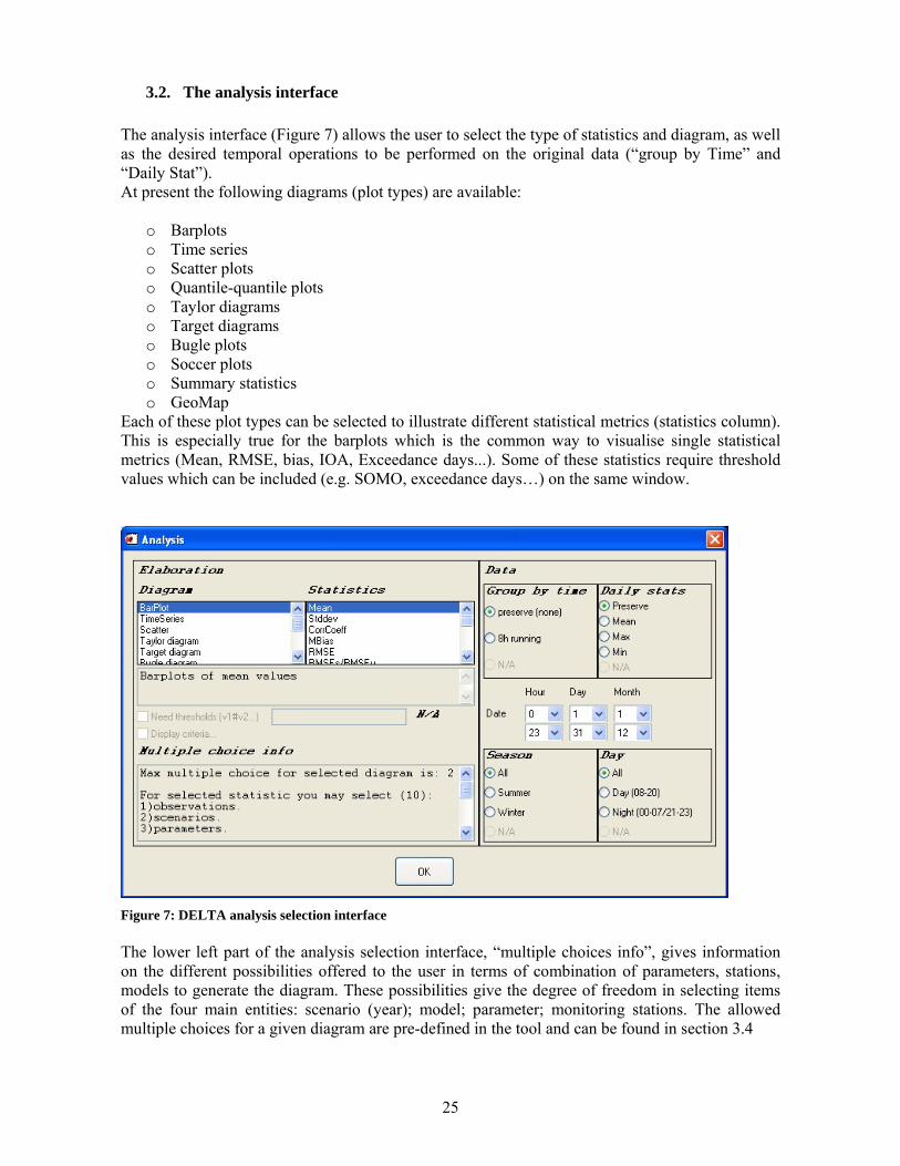
3.2. The analysis interface The analysis interface (Figure 7) allows the user to select the type of statistics and diagram, as well as the desired temporal operations to be performed on the original data (“group by Time” and “Daily Stat”). At present the following diagrams (plot types) are available:

o Barplots o Time series o Scatter plots o Quantile-quantile plots o Taylor diagrams o Target diagrams o Bugle plots o Soccer plots o Summary statistics o GeoMap

Each of these plot types can be selected to illustrate different statistical metrics (statistics column). This is especially true for the barplots which is the common way to visualise single statistical metrics (Mean, RMSE, bias, IOA, Exceedance days...). Some of these statistics require threshold values which can be included (e.g. SOMO, exceedance days…) on the same window.

Figure 7: DELTA analysis selection interface The lower left part of the analysis selection interface, “multiple choices info”, gives information on the different possibilities offered to the user in terms of combination of parameters, stations, models to generate the diagram. These possibilities give the degree of freedom in selecting items of the four main entities: scenario (year); model; parameter; monitoring stations. The allowed multiple choices for a given diagram are pre-defined in the tool and can be found in section 3.4

26

On the right side of the analysis selection interface, time operations can be chosen to be performed on the selected modelled-observed data pairs, i.e.:

• Time series kept as originally formatted (1h) or 8h running average • Statistical operation applied for each day: mean, max or min. • Season selection: choice between summer, winter and entire year • Hour selection: night time hours, daylight hours or entire 24h day.

Note that for some statistics, e.g. exceedance days, some of these flags will be automatically filled to the adequate values.

3.3. The main graphical interface The main DELTA graphical interface, result of options previously selected by the user, is presented in Figure 8. The screen is divided into two main areas:

• The left side memorises the user choices which lead to the generation of a given diagram. • The right side hosts the diagram and accompanying legend (which also summarizes the

options selected by the user). Only one diagram is shown at a time (i.e. no multiple windows).

Figure 8: DELTA main graphical window. The example shown is the target plot for maximum daily 8h mean O3 as calculated by two models at a single station

27

3.4. Multiple choice options These options are detailed separately for the two main applications of DELTA, i.e. assessment and planning. Note that for the time being focus has been put on assessment type of applications. The choice of available options for planning applications will be enlarged in a next development stage version of the software. Examples of available diagrams obtained with different options are provided in Figure 9 Assessment applications

Diagram Statistics visualized Multiple choice options allowed M P O M-P M-O P-O Bar_plots Mean Stddev CorrCoeff Bias RMSE

RMSEs/RMSEu

IOA

ExcDays

MFB

MFE

GME

TARGET=RMSE/StddevO

RDE

RPE

Scatter plots Mean Stations All points Time series Taylor Target Buggle Soccer Q-Qplot Mean Stations All values Summary Statistics

GeoMap

Table 2: Multiple choice options allowed (Grey filled boxes) for diagrams and related statistics (assessment applications). For example the grey box M-S for the scatter plots indicate the possibility to overlay results from different scenarios and different models on the scatter diagram. “S” stands for Scenario (year), “M” for models, “O” for observation stations and “P” for parameters).

28

Planning applications

Diagram Statistics visualized Multiple choice options allowed S M P O S

M S P

S O

M P

M O

P O

Bar_plots Mean Stddev ExcDays

Time series Table 3: Multiple choice options allowed (Grey filled boxes) for diagrams and related statistics (planning applications). Symbols as above

Plot type Option 1 Option 2 Time Series Left: Obs. vs. Model Right: Obs. ss. 2 models

Scatter Left: All stations for 1 model and 1 parameter, 1 scenario. Right: same but for 2 parameters (O3 and PM10)

Taylor Left: All stations for 1 model and 1 parameter, 1 scenario. Right: same but for 2 parameters (O3 and PM10)

29

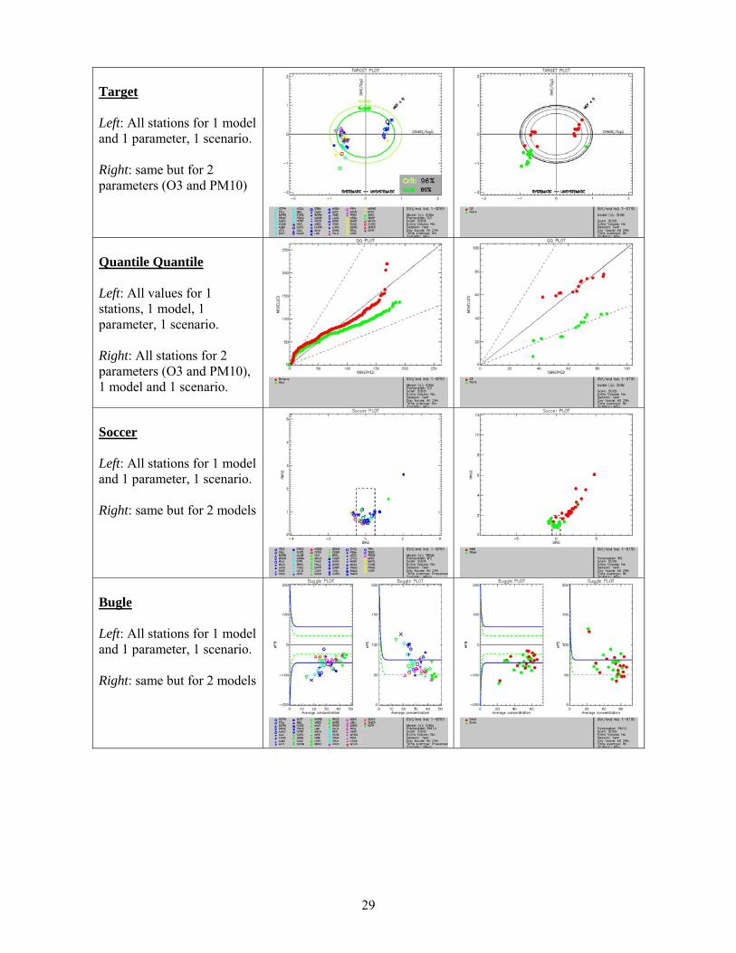
Target Left: All stations for 1 model and 1 parameter, 1 scenario. Right: same but for 2 parameters (O3 and PM10)

Quantile Quantile Left: All values for 1 stations, 1 model, 1 parameter, 1 scenario. Right: All stations for 2 parameters (O3 and PM10), 1 model and 1 scenario.

Soccer Left: All stations for 1 model and 1 parameter, 1 scenario. Right: same but for 2 models

Bugle Left: All stations for 1 model and 1 parameter, 1 scenario. Right: same but for 2 models

30

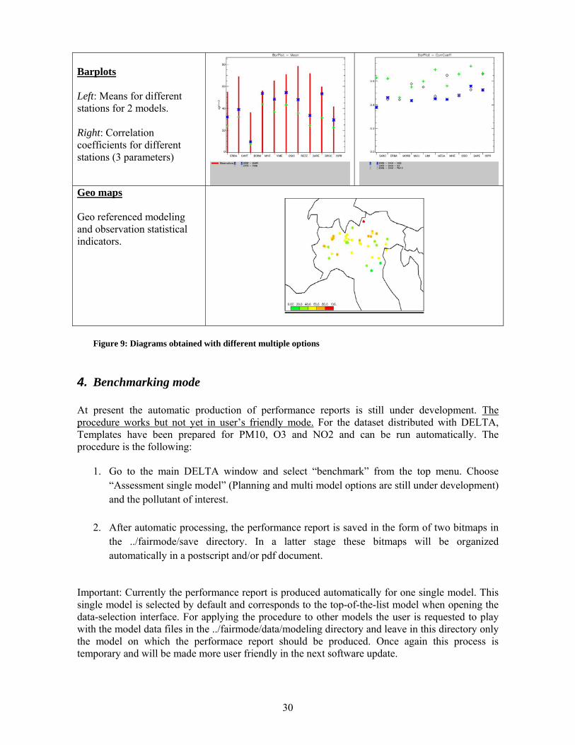
Barplots Left: Means for different stations for 2 models. Right: Correlation coefficients for different stations (3 parameters)

Geo maps Geo referenced modeling and observation statistical indicators.

Figure 9: Diagrams obtained with different multiple options

4. Benchmarking mode At present the automatic production of performance reports is still under development. The procedure works but not yet in user’s friendly mode. For the dataset distributed with DELTA, Templates have been prepared for PM10, O3 and NO2 and can be run automatically. The procedure is the following:

1. Go to the main DELTA window and select “benchmark” from the top menu. Choose “Assessment single model” (Planning and multi model options are still under development) and the pollutant of interest.

2. After automatic processing, the performance report is saved in the form of two bitmaps in

the ../fairmode/save directory. In a latter stage these bitmaps will be organized automatically in a postscript and/or pdf document.

Important: Currently the performance report is produced automatically for one single model. This single model is selected by default and corresponds to the top-of-the-list model when opening the data-selection interface. For applying the procedure to other models the user is requested to play with the model data files in the ../fairmode/data/modeling directory and leave in this directory only the model on which the performace report should be produced. Once again this process is temporary and will be made more user friendly in the next software update.

31

5. Distributed Dataset: Po-Valley This dataset contains the results from a model inter-comparison exercise performed by six air quality models for year 2005. The model domain covers the Po Valley (Italy) with at 6 x6 km2

resolution (95x65 cells) grid. Pollutant concentrations have been simulated by 5 transport chemical (CHIMERE, TCAM, CAMX, RCG, MINNI ) and 2 meteorological models (MM5 and TRAMPER). More details about the POMI exercise can be found at the POMI website http://aqm.jrc.it/POMI/index.html. Observations from 63 monitoring sites located in the Po Valley are also provided. Sites have been classified in regions and station types (suburban, urban and rural).

6. Limitations of the current release of DELTA The current version of this tool has been developed and tested on Windows machines only. It requires a version of the IDL Virtual Machine for windows. Further versions of the tool for Mac and Linux environments will be tested and released in the future. The tool treats monitoring stations individually: groups of stations clustered as a single entity are not allowed for now. Meteorology and air quality data are treated separately. The combined analysis of meteorological and air quality parameters is permitted only if modeled and monitoring files are prepared accordingly.

7. Examples of required CPU The CPU time mainly depends on the number of monitoring stations and models in the dataset as well as on the choice of the multiple option analysis. An estimate has been performed for the POMI dataset containing approximately 60 stations, 5 models and 1 parameter (O3 8-hour daily max) on a Windows XP Machine (Intel Core Quad CPU, 2.83 Ghz, 3.25GB of RAM). Results for some diagrams are reported in table 4.

Diagram Computing time (approx.) Target 1 min Taylor 3 min. and 30 sec. Bugle 2 min and 40 sec.

Soccer 3 min and 20 sec. Scatter 1 min and 15 sec.

Table 4: Estimate of the CPU time for the visualization of the main diagrams in Delta