the deep space network progress report 42-44
TRANSCRIPT

(NASA-M--'157110) THE DFEr SPACE 'NETWORKProgress Report, Jan. Peb. 1978 (Jetrropulosion 1,ab.) 3110 HC A14/MF A01
CSCL 22DG3/12
V78-24212THFUN78-24244Unclas21439
The Deep Space NetworkProgress Report 42-44
January and February 1978
National Aeronautics andSpace Administration
Jet Propulsion LaboratoryCalifornia Institute of TechnologyPasadena California 91103
"o
https://ntrs.nasa.gov/search.jsp?R=19780016269 2018-03-26T22:51:30+00:00Z

The Deep Space NetworkProgress Report 42-44
January and February 1978
April 15, 1978
National Aeronautics andSpace Administration
Jet Propulsion LaboratoryCalifornia Institute of TechnologyPasadena California 91103

Preface
Beginning with Volume XX, the Deep Space Network Progress Report changed fromthe Technical Report 32- series to the Progress Report 42- series. The volume numbercontinues the sequence of the preceding issues. Thus. Progress Report 42 .20 is thetwentieth volume of the Deep Space Network series, and is an uninterrupted follow-on toTechnical Report 32 . 1520. Volume XIX.
This report presents DSN progress in night project support, tracking and dataacquisition (TDA) research and technology, network engineering, hardware and softwareimplementation, and operations. Each issue presents material in sonic, but not all, of thefollowing categories in the order indicated.
Description of the DSN
Mission SupportOngoing Planetary/Interplanetary Fliglt; ProjectsAdvanced Plight Projects
Radio Astronomy
Special Projects
Supporting Research and TechnologyTracking and Ground-Based NavigationCoinnlUnie,itioils—Spacceraft/GroundStation Control and Operations TechnologyNetwork Control and Data Processing
Network and Facility Engineering and ImplementationNetworkNetwork Operations Control CenterGround CommunicationsDeep Space StationsQuality Assurance
OperationsNetwork OperationsNetwork Operations Control CenterGround CommunicationsDeep Space Stations
Program PlanningTDA Planning
In each issue, the part entitled "Description of the DSN" describes the functions andfacilities of the DSN and may report the current configuration of one of the five DSNsystems (Tracking, Telemetry, Command, Monitor & Control, and Test & Training).
The work described in this report series is either performed or managed by theTracking and Data Acquisition organization of JPL for NASA.
Ill

Page intentionally left blank
Contents
DESCRIPTION OF THE DSN
DSN Functions and Facilities . . . . . . . . . . . . . . . . . 1N. A. Renxetti
DSN Test and Training System, Mark III .77 . . . . . . . . . . . 4H. C. ThormanNASA Code 311.03.43.10
MISSION SUPPORT
Ongoing Planetary/Interplanetary Flight Projects
Voyager Support . . . . . . . . . . . . . . . . . . . . . . 16R. MorrisNASA Code 311.03.22.20
Viking Extended Mission Support . . . . . . . . . . . . . . . 34T. W. HoweNASA Code 311.03.21.70
Pioneer Mission Support . . . . . . . . . . . . . . . . . . 44T. P. AdamskiNASA Code 311.03.21-90
Helios Mission Support . . . . . . . . . . . . . . . . . . . 50P. S. Goodwin, W. N. Jensen, and G. M. RockwellNASA Code 311.03-21.50
SUPPORTING RESEARCH AND TECHNOLOGY
Tracking and Ground-Based Navigation
An Alternate Technique for Near-Sun Ranging . . . . . . . . . . 54J. W. l_aylandNASA Code 310.10.61.08
The Tone Generator and Phase Calibration inVLBI Measurements . . . . . . . . . . . . . . . . . . . . 63J. B. ThomasNASA Code 310-10.60.06
An Analysis of Viking S-X Doppler Measurements of SolarWind Columnar Content Fluctuations . . . . . . . . . . . . . 75P. S. CallahanNASA Code 310.10.60.05
V

A Method for Measuring Group Time Delay Through aFeed Horn . . . . . . . . . . . . . . . . . . . . . . . . 82T. Y. Otoshi, P, B. Lyon, and M. FrancoNASA Code 310-10-61-08
Communications—Spacecraft/Ground
An Analysis of Alternate Symbol Inversion for ImprovedSymbol Synchronization in Convolutionally Coded Systems . . . . . 90L. D. Baumert, R. J. McEliece, and H. van TiiborgNASA Code 310.20.67.11
A Prototype DSN X-S Band Feed: DSS 13 FirstApplication Status . . . . . . . . . . . . . . . . . . . . . 98W. F. WilliamsNASA Code 310.20.65.05
LAASP 100-m Antenna Wind Performance Studies . . . . . . . . 104R. Levy and M. S. KatowNASA Code 310.20.65.13
A Public-Key Cryptosystem Based On Algebraic CodingTheory. . . . . . . . . . . . . . . . . . . . . . . . . . 114R. J. MCElleGeNASA Code 310.10.67-11
Tracking Loop and Modulation Format Considerations forHigh Rate Telemetry . . . . . . . . . . . . . . . . . . . . 117J. R. LeshNASA Code 310.20.67.13
Station Control and Operations Technology
Development Support—DSS 13 S-X UnattendedSystems Development . . . . . . . . . . . . . . . . . . . 125E. B. JacksonNASA Code 310.30.68-10
Network Control and Data Processing
The DSN Standard Real-Time Language . . . . . . . . . . . . . 131R. L. Schwartz, G. L. Fisher, and R. C, TauswortheNASA Code 310.40.72.05
V1

NETWORK AND FACILITY ENGINEERINGAND IMPLEMENTATION
Network
On Decoding of Reed-Solomon Codes Over GF(32)and GF(64) Using the Transform Techniques of Winograd. . . . . . 139I. S. Reed, T. K. Truong, and B. Benja^,,thritNASA Code 311.03.42.05
Electron Density and Doppler RMS Phase Fluctuation in theI nner Corona . . . . . . . . . . . . . . . . . . . . . . . 172A. L. BermanNASA Code 311.03.43.10
The DSS Radio Science Subsystem—Real-TimeBandwidth Reduction and Wideband Recordingof Radio Science Data . . . . . . . . . . . . . . . . . . . 180A. L, BermanNASA Code 31103.43.10
Solar Wind Density Fluctuation and the Experiment toDetect Gravitational Waves in Ultraprecise Doppler Data . . . . . . 189A. L. BermanNASA Code 311.03.43.10
Solar Wind Turbulence Models Evaluated via Observationsof Doppler RMS Phase Fluctuation and SpectralBroadening in the Inner Corona . . . . . . . . . . . . . . . . 197A. L. BermanNASA Code 311.0343.10
On the Suitability of Viking Differenced Range to theDetermination of Relative Z-Distance . . . . . . . . . . . . . . 203F. B. WinnNASA Code 311.03.42-54
Ground Communications
CCIR Papers on Telecommunications for DeepSpace Research . . . . . . . . . . . . . . . . . . . . . . 211N. F. deGrootNASA Code 311.06.60.00
V11
Deep Space Stations
Development of a Unified Criterion for SolarCollector Selection . . . . . . . . . . . . . . . . . . . . . 224F. L. LansingNASA Corse 311.0341 ,08
Implementation of Automated Fault Isolation Test Programsfor Maximum Likelihood Convolutional Decoder (MCD)Maintenance . . . . . . . . . . . . . . . . . . . . . , 236M. E. AlbardaNASA Code 311.03.44.11
Performance of Solar-Powered Vapor-Jet RefrigerationSystems with Selected Working Fluids . . . . . . . . . . . . . 245V. W. Chai and F. L. LansingNASA Code 311.03.41.08
OPERATIONS
Network Operations
Voyager Near Simultaneous Ranging Transfers. . . , . . . . . . 252G. L, SpradlinNASA Code 311.03-13-20
Some Data Relationships Among Diverse Areas of theDSN and JPL . . . . . . . . . . . . . . . . . . . . . . . 260R. M. SmithNASA Code 311.03.13-25
A New, Nearly Free, Clock Synchronization Technique .W. H. H ietzkeNASA Code 311.03-13.20
Deep Space Stations
Tracking Operations During the Voyager 2 Launch Phase.J. A. Wackley and G. L. SpradlinNASA Code 311.03-13.20
. . . 268
273
viii
PROGRAM PLANNING
An Effective Procurement and Financial ManagementReporting System . . . . . . . . . . . . . . . . . . . . . 28)J. B. Rozek anti F. R. WoccoNASA Code 311-03 .3 2-10
Ix

13SN Progreau Report 42 AA
January and February 1978
1
Network Functions and FacilitiesN. A. Fenzetti
Office of Tracking and Data Acquisition
The objectives, functions, and organization of the Deep Space Network aresto nrarized, sleep space station, ground conman cation, and network operations controlcapabilities are described.
The Deep Space Network was established by the NationalAeronautics and Space Administration (NASA) Office ofSpace Tracking and Data Systems and is under the systemmanagement and technical direction of the Jet PropulsionLaboratory (JPL). The network is designed for two-waycommunications with unmanned spacecraft traveling approxi-mately 16,000 kiln (10,000 miles) from Earth to the farthestplanets and to the edge of our solar system, It has providedtracking and data acquisition support for the following NASAdeep space exploration projects. hanger, Surveyor, MarinerVenus 1962, Mariner Mars 1964, Mariner Venus 1967, MarinerMars 1969, Mariner Mars 1971, and Mariner Venus-Mercury1973, for which JPL has been responsible for the projectmanagement, the development of the spacecraft, and tileconduct of mission operations, Lunar Orbiter, for which theLangley Research Center carried out the project management,spacecraft development, and conduct of mission operations;Pioneer, for which Ames Research Center carried out theproject management, spacecraft development, and conduct ofmission operations; and Apollo, for which the Lyndon B.Johnson Space Center was the project center and the DeepSpace Network supplemented the Manned Space Flight Net-work, which was managed by ale Goddard Space FlightCenter. The network is currently providing tracking and dataacquisition support for Hellos, a joint U.S./West Germanproject; Viking, for which Langley Research Center providesthe project management, the Lander spacecraft, and conducts
mission operations, and for which JPL provides the Orbiterspacecraft; Voyager, for which JPL provides project manage-ment, spacecraft development, and conduct of missionoperations; and Pioneer Venus, for which the Ames ResearchCenter provides project management, spacecraft development,and conduct of mission operations. The network is adding newcapability to meet the requirements of the Jupiter OrbiterProbe Mission, for which JPL provides the project manage•ment, spacecraft development and conduct of missionoperations.
The Deep Space Network (DSN) is one of two NASAnetworks. The other, tile Spaceflight Tracking and DataNetwork (STDN), is under the system management andtechnical direction of the Goddard Space flight Center(GSFC). Its function is to support manned and unmannedFarth•orbiting satellites. The Deep Space Network supportslunar, planetary, and interplanetary flight projects.
From its inception, NASA has had the objective ofconducting scientific investigations throughout the solar sys-tern. It was recognized that in order to meet this objective,significant supporting research and advanced technology devel-opment must be conducted in order to provide deep spacetelecommunications for science data return in a cost effectivemanner. Therefore, the Network is continually evolved to keeppace with the state of tine art of telecommunications and data

handling It wow also recoil tuied curly tha close coordination
would be needed hetveert the requirements tut' tilt' Iiip!lrt
projects Ion data return and tl ►e calmbilitle^, headed u 1 th eNetwork. Tins close vollaboratum was ettected by tite appoint.
mont of it I tacking and Datir Systems hot° lager as part 11 t thetl ►gllt project te,un from the initiation of the plolect to theend of the mission. By this process. re kill iretnetlis wereIdentified early cnuul,h It) provide funding and inlplamelta•uolh nn time for t► se by the flight project in its flight Phase.
As ot'JuI.N 19 77 -2 , NASA undertook th change i ► h the u ► terfacebetween the Network and the flight projects. prior to thattime, since I January 1994. tit to consisting,, tit dieDeep Space Stations and the Ground Communications
Facility, the Network hard gist) included the mission controland eunlputirtt*, facilities and provided the etluipmen : themission support areas tot tiro conduct of minion op.r ns.
The latter facilities were housed in a building at JP1, knu: 'tl asthe Space Flight Operations Facility (SFOF). The interlaceahang was to accunimodate a hardware interface between theSupport of the network operations control functions wid thosetit ' the mission contrul and computing I'll lie( ious. This resulted
to the flight projects assuming the coemi/ante of the large
general-purpose digital computers which were used for both
network processing and mission data processing. They also
asstnned Cognizance of all tit' rile equipillent ill Ile flightoperations facility for display and communications necessary
cur the conduct of mission operations. The Network the_tundertook the development of hardware and computer soft.ware necessary to do its network operations control andmonitor functions tit computers. A characteristic ofthe new interface is that the Network provides direct data flow
it) auA from the stations; nainlely, metric data, science and
engineering telemetry, ,end such network monitor tiata as are
useful to the flight project. This is dune via appropriate ground
communication equipment to mission operations centers.
wherever the y may he.
T'ha principal deliverables to the users of the Network are
carried out by data system configurations as follows:
The DSN Tracking System generates radio metric data.
i.e.. angles, onc- lint) two-way doppler and range, and
transmitb raw data to Mission Control.
• The DSN Telemetry System receives. decodes, records,
anti retransmits engineering and scientific data generated
ill tile spaceeraft to Mission Control.
0 The DSN Command System accepts spacecraft com.
elands from mission Control and transmits the com-
mallds via the Ground C'onunlunication Facility to a
Deep Space Station. The commands are then radiated to
the spacecraft ill order to initiate: spacecraft functions in
flight.
• I lie I)SN Radio Scrc i we W,tem p'enetato radio wlence
data, he.. the IregtlencV , a1111a htilde of spueoalttratimi rtted sgnal ,, attested by pa,,sage throurh medla
sued as the solar corrna. planetary atinwpheres, and
planetary ling,. and transmits this data it) Mi5siolr
Control.
The data system conlig,trattllll',testiigt, traminh,
and network operations control ti ► nctions are as bellows:
• 'Hie DSN 'Monitor and Control System instruments.
transtnits, records. and displays those patanleters of theDSN necessary to verity contiguration and validate theNetwork. It provides the tools necessary tier Network
Operations personnel I, control turd monitor the Net-work and interface with flitht project mission controlpersonnel.
The DSN Test and 'Training; System generates and
controls , .Mated data to support development, test.
training and fault Isolation within tilt! DSN. it partici-
pates in mission simulation with flight projects.
The capabilities deeded to carry oil( the above functionshave evolved tit technical areas:
( i ) The Thep Space Stations. which are distributer( agroundFarth ant*, which, prior it) 1964. formed part of theDeep Space Instrumentation Facility. 'The technologyinvolved ill these stations is strongly relatedto the state of the art of telecommunications andflight-ground desigln considerations. and is almost com.pletely multimission ill character.
(2) The Ground Communications Facility provides the
capability required for the transmission, rwceptkln. and
monitoring of Farth-based, point-to-point eommunica•
tions between the stations and the Network Operations
Control Center at AT. Pasadena, and to the .11T Nlis-
sion Operations Centers. Four communications dis.
ciplines are provided: teletype, voice, high=speed, and
wideband. The Ground Communications Facility uses
the capabilities provided by cotnunon carriers through-
out the world, engineered into an integrated system by
Goddard Space Flight Comm and controlled liom thecanlmunicationx Center IOCated in tine Space Flight
Operations facility (Building 230) at JPI..
'The Network Operations Control Center is the functional
entity for centralized operational control of the Network and
interfaces with the users. It has two separable functional
elements; namely, Network Operations Control and Network

vala l trank',an it 11W tE6tlatSA 4 t ► h tit t1iE' Noln,"Is t POWIit9l't
1'et;ittt tl and etv l ttlillallt I II I I I NOM ink "alpp=tll ht involOnilillitillotil la 10'tit"i y OIL n5t`th-
♦ 1 Itl ► c'atit tn ttl tilt' Notty ttnh dalrl pit t4t", tc^, t'ttlllplltlllf',
F"alla111111^ tit I '":netale :Ill "I Middle" and 1111111"" tetitilietlfor Nomoth ttpetalltttl`,
0 1 Illvat ►utl of Nom ink data tt111pI1thilti.apaltlllt y it, ati:r ylk, alltl validate tile perlt ► t mkv of all
Net" Ink system",,
ille pefht tllil:'1 %%]Itt ;iltlN alit tilt' ahme flni411 m ail' ltteatthl
in the Spaue 1'Q1 t)p><tt,t mms Wit,. w1me minsmi a upt"Ia-mom hill, m qh ;Ill° called ttnl 11 'XitraUt 111e`1"I plttlea y Net®Synth pelbttunel me MOM hN an Opeiatum Otuitittl ('hict!
lb'. tuurtituis ttf tltc'tit`t ►yttlh Data 1'tueewtinilt ;Ifs'
• 10"mur tit data Imod lay 'itiCl4tatk ttlleratl"til'ot°ttntT"+(h it. w4d and alml y ,11 ttt 11 ►t` 4"tt5t^tls,
• Dvgllak tit tilt" Nof%y tsth Olvialiow) Colitital Altai ttt data
pitttosed tit theNetuuth Ilata 1'ittsv ,oiur Ate,:t.
0 lnwrlue Witll dt>111111Inniatums CUEt N ba Inp ►!t tit and
Itnlput 1st % nl till' Nemmk 141a l i lt t t,=emuir Am.
Data aini production Ill tilt' Itltefiiledlilte dataleo"ds.
111e polmnmel Mltt caliN out these 11111olt t lly are Iueafodappmunalov 00 nletelr, trtttll tilt° Spawe Hiltlit Operations
Will, The quipnu"Ilt t: tulAst ," ttt tor real-
ume data system 111t tnit ttring. two XDS Sq!ina ' ,,. thq)hkt .111MMOUC tape teolideN anti applttpli; lt! 11110fHe etluillnlenlI,y ith tile 'mound tlat,t comilluliivaticilm
3

DSN Progress Report 42.44
January and February 1978
IN 78 -24214
DSN Test and Training System, Mark III-77H. C. Thorman
TDA Engineering Office
Implementatimi of the DSN Test and Training ,System, A1ark 111. 77, throughout firenetwork is nearing completion. The :ftk 11177 system is configured to support DR-I"
testing and training for the Pioneer-Venus 1978 missloit and all on-going, in-ji. imisslons. DSN Test and Training S;vstem capabilities include ,limetions performed in tapeDeep Space Stations, Ground Communications Facility, and Network Operations ControlCen ter,
I. System Definition Figure 1 describes the functions, elements, and interfaces ofthe system. Tills article updates the system description pub.
A. General lisped in Ref. 1,
The DSN Test and Training Systow is a multiple-missionsystem whieti supports Network-wide testing and training byinserting test signals and data into subsystems of the DeepSpace Stations (DSS), the Ground Communications Facility(GCF), and the Network Operations Control Center (NOCC).The system includes capabilities for:
(1) On-site testing of the DSS portion of eacli DSN system,
(2) Local testing of the NOCC portion of eacli DSNaysteni.
(3) End-to-end testing of each DSN system, including DSS,GCF, and NOCC functions.
B. Key CharacteristicsDesign goal icey cliaracteristics of the DSN Test and Train
ing System are:
( I ) Capability to function without alteration of DSN oper-ational configuration.
(2) Utilization of mission-independent equipment for DSNtesting and training functions.
(3) Capability to exercise NOCC, GCF, and DSS simulta-neously, for end-to-end testing of each USN system,
4

(4) Capability to supply test data to all DSN systemssimultaneously,
(5) Capability to load Network with combination of actualand simulated data streams.
(6) Accommodation of flight-project-supplied simulationdata via GCE,
(7) Accommodation of other data sources, as follows:
(a) Spacecraft test data via JPL Compatibility TestArea (CTA 2 1) .
(b) Spacecraft prelaunch data via Merritt Island,Florida, Spacecraft Compatibility-Monitor Station(STDN (MIL 71)).
C. System UsageMajor testing and training activities supported by the DSN
Test and Training System are summarized below;
(1) Prepass and pretest calibrations, readiness verifications,and fault isolation.
(2) DSN implementation activities and performance testingof DSN systems, DSS subsystems, and NOCC sub-systems.
(3) DSN operational verification tests to prepare for mis.sion support.
(4) Flight project ground data system tests and missionsimulations.
II. Mark III-77 System ImplementationA. Status
A functional block diagram showing the data-flow andsignal-flow paths of the DSN Test and Training System, Mark111.77, is shown in Fig. 2. implementation of the Mark I11-77system throughout the network will have been completedwhen DSS 11 returns to operation in the latter part of March,1978.
Upgrading of the DSS portions of this system has been apart of the DSN Mark III Data Subsystems (MDS) implementa-tion project, which began in 1976.
S. Mission SetThe Mark III-77 configuration of the DSN Test and Train-
ing System includes all elements of the system required forsupport related to the following mission set:
(1) Viking Orbiters 1 and 2 and Viking Landers 1 and 2(extended mission).
(2) Pioneers 6 through 9.
(3) Pioneers 10 and 11,
(4) Helios I and 2.
(5) Voyagers I and 2 (including planetary encounters).
(6) Pioneer-Venus 1978 (PV '78) Orbiter and Multiprobe,
C. New CapabilitiesThe following modifications and additions upgraded the
system to the Mark 111.77 configuration:
(1) Modification of the DSS Simulation Conversion Asse,n-bly (SCA) to provide capability for short-constraint-length convolutional coding of simulated Voyager telem.etry data and long-constrain Wength convolutionalcoding of simulated PV '78 telemetry data, as describedin Ref, 2.
(2) Additional program software for the XDS-910 Simula-tion Processor Assembly (SPA), to control new SCAequipment, to generate simulated Voyager and Pioneer-Venus telemetry 1ata patterns, and to convert project-supplied data fiom GCF high-speed and wideband datablocks into serial data streams, as described in Ref. 2.
(3) New program software to perform the System Perfor-mance Test (SPIT) functions of on-site closed-loop per-formance testing and validation of the Tracking, Telem-etry, Command, an+1 Monitor and Control Systems.
(4) Configuring of the GCF Communications Monitor andFormatter (CMF) backup minicomputer to provideinterfaces required for the SPT functions.
(5) Implementation of the Network Control Test andTraining Subsystem in the Network Operations ControlCenter (Block III).
(6) Implementation of special test and training equipmentin the Receiver-Exciter Subsystem at DSS 14 and 43,to generate four carriers simulating the expected dopp-ler profile and sequence characteristics of the carriersto be received from the Pioneer-Venus atmosphericentry probes. The design of this simulator is describedin Ref. 3.
III. Deep Space Station FunctionsA. DSS Test and Training Subsystem
The functions of the DSS Test and Training Subsystem andthe ref ted interfaces are shown in Fig. 3.
(1) Telemetry simulation and conversion. The telemetrysimulation and conversion functions are performed by
5

the Simulation Processor Assembly and the SimulationConversion Assembly, as diagrammed in Fig. 4. Digitaland analog capabilities are itemized in Tables 1 and 2,respectively.
(2) System performance test functions. The system perfor.mance test functions are performed by the SPT Soft.ware Assembly, as diagrammed in Fig. 5.
B. Receiver-Exciter SubsystemThe Receiver-Exciter Subsystem provides the following test
and training functions:
(1) Generation of sirnuiated S-band and X-band downlinkcarriers.
(2) Modulation of telemetry subcarriers from the SCAonto simulated carriers,
(3) Variable attenuation of simulated downlink carriersignal level under control of the SPA.
(4) Translation of S-band exciter uplink frequencies toS-band and X-band downlink frequencies, for TrackingSystem calibrations and performance testing.
(5) Generation of simulated Pioneer-Venus entry probecarriers at DSS 14 and 43.
C. Antenna Microwave SubsystemThe Antenna Microwave Subsystem provides the following
test and training functions:
(l) Routing of simulated downlink carriers to masers and/or receivers.
(2) Mixing of simulated S-band downlink carriers.
D. Transmitter SubsystemThe Transmitter Subsystem includes provision for feeding
the transmitter output into a dummy load to support Com-mand System and Tracking System test operations.
E. Frequency and Timing SubsystemThe Frequency and Timing Subsystem provides the follow-
ing support functions to the DSS Test and Training Sub-system:
(I) Time code and reference frequencies.
(2) Generation and distribution of a simulated time signalwhich can be substituted for the true GMT input to thevarious DSS subsystems. This capability is provided forrealistic, mission simulations in support of flight projecttesting and training activities.
IV. Ground CommunicationsFacility Functions
The DSN Test and Training System utilizes the GroundCommunications Facility Subsystems for communicating dataand Information between the Network Operations ControlCenter (NOCC) or any Mission Operations Center (MOC) andthe Deep Space Stations,
A. High-Speed Data SubsystemThe Nigh-Speed Data Subsystem provides the following:
(1) Transmission of text messages, control messages, low-to medium-rate simulated telemetry data, and simu-lated command data to any DSS from the NOCC orfrom any MOC.
(2) On site loop-back of test data for systems performancetesting and readiness verifications in the DSS.
B. Wideband Data SubsystemThe Wideband Data Subsystem provides the following:
(1) Transmission of simulated high-rate telemetry data tothe 64-m s! ►bnet (DSSs 14, 43, and 63), the Compati-bility Test Area (CTA 21), in Pasadena, California, andSTDN (MIL 71) at Merritt Island, Florida, from theNOCC or from any MOC having wideband capability.
(2) On-site loop-back of test data for telemetry systemperformance testing and readiness verification in thoseDeep Space Stations which have wideband capability.
C. Teletype and Voice SubsystemsThe Teletype and Voice Subsystems provide communica-
tion of information for purposes of test coordination andmonitoring of the DSN Test and Training System status.
V. Network Operations Control CenterFunctions
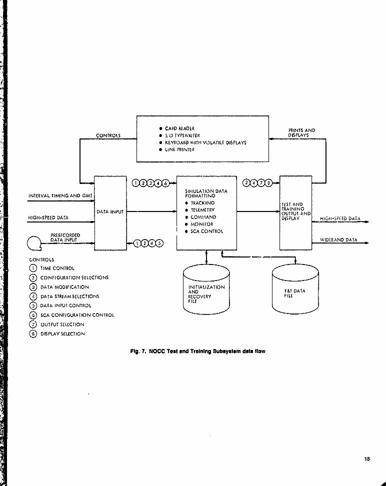
A. NOCC Test and Training SubsystemFunctions and interfaces of the NOCC Test and Training
Subsystem are shown in Fig. 6. Subsystem data flow is dia-grammed in Fig. 7. Test and training capabilities presentlyimplemented in the Network Operations Control Center are asfollows:
(1) Selection of stored data blocks and output to the DESfor system readiness verification.
(2) Off-line generation of recordings of high-speed datablocks for testing of the real-tine monitors in the
6

NOCC Tracking, Telemetry, Command, and MonitorSubsystems.
(3) Output of text and control messages to the DSS forremote configuration and control of the SPA and SCAIn support of DSN Operational Verification Tests,
B. DSN Test and Training System Control Console
A DSN Test and Training System Control Console in theNetwork Data Processing Area provides keyboard, card reader,::agnetic tape unit, volatile display, and character printer foroperation of the Test and Training System separate from theoperations of the other DSN Systems.
References
1. Thorman, H. C., "DSN Test and Training System, Mark 111 .77," in The Deep SpaceNetwork Progress Report 42-38, pp. 4 . 15, Jet Propulsion Laboratory, Pasadena,California, April 15, 1977,
2. Yee, S. H., "Modification of Simulation Conversion Assembly for Support of VoyagerProject and Pioneer-Venus 1978 Project," in The Deep Space Network Progress Report42-39, pp. 100. 108, Jet Propulsion Laboratory, Pasadena, California, June 15, 1977.
3. Friedenberg, S. E., "Pioneer Venus 1978 Multiprobe Spacecraft Simulator," in TheDeep Space Network Progress Report 42-38, pp. 148 . 151, Jet Propulsion Laboratory,Pasadena, California, April 15, 1977.
7

Table 1. DSS Test and Training Subsystem digital telemetry simulation capabilities
Capability 26-meter DSS, MIL 71 64-meter DSS, CTA 21
Maximum number of simultaneous real-time data 2 channels Viking extended mission, 4 channelsstreams
Other missions, 3 channels
Di-orthogonal (32, 6) comma-fro: block coding Viking, 2 channels Viking, 3 channels
Other missions, none Other missions, none
Short-constraint-length convolutional coding Mariner Jupiter-Saturn, rate = 1/2, Mariner Jupiter-Saturn, rate = 1/2,(k=7, r= 1/2 or 1/3) 2 channels 3 channels
Future missions, rate = 1/3, Future missions, rate = 113,1 channel 2 channels
Long-constraint-length convolutional coding Helios, I channel
Helios, I channel(k=32, r=1/2) Pioneer 10/11, 2 channels Pioneer 10/11, 2 channels
Pioneer Venus, 2 channels Pioneer Venus, 3 channels
Variable :ate control
Selection of discrete rates
1 bps to 600 ksps on1 channel
I bps to 190 ksps on I additionalchannel
8-1/3, 33.1/3 bps on each of2 channels (for Viking)
1 bps to 600 ksps on2 channels
I bps to 190 ksps on 1 additionalchannel
8-1/3, 33 . 1/3 bps on each of3 channels (for Viking)
Table 2. DSS Test and Training Subsystem analog teleme
Capability 26-meter DSS, MIL 71
Data and subcarrier signal conditioning, phase- 2 subcarriersshift keyed modulation
Subcarrier frequency output 512 IN to 1.25 MHz, 1 /4-lizresolution
dry simulation capabilities
64-meter DSS, CTA 21
Viking extended mission, 4 subcarriers
Other missions, 3 subcarriers
512 Hz to 1.25 MHz, 1/4-Hzresolution
Modulation-index angle control
Subcarrier mixing and downlink carrierbiphase modulation
Downlink carrier signal level
Controllable from 0 to 89 deg oneach Subcarrier
Single or dual subcarriers onto eachof 2 S-band test carriers or 1S-band and I X-band
Attenuation of 0 to 40 dB on eachtest carrier output
Controllable from 0 to 89 deg on eachSubcarrier
Single or dual subcarriers onto each of3 test carriers or 2 S-band and1 X-band
Attenuation of 0 to 40 dB on eachtest carrier output
eORIGINAL PAGE IbOF P001l (QUALITY

DSN SYSTEM INTERFACES
OPERATIONS INTERFACES
LOCATIONS OF SYSTEM ELEMENTS
• DEEP SPACE STATIONS
• DSS TEST & TRAINING SUBSYSTEM
• RECEIVER-EXCITER SUBSYSTEM
• ANTENNA MICROWAVE SUBSYSTEM
• TRANSMITTER SUBSYSTEM
• FREQUENCY & TIMING SUBSYSTEM
• GROUND COMMUNICATIONS FACILITY
• NETWORK OPERATIONS CONTROL CENTER
• NOCC TEST & TRAINING SUBSYSTEM
• DSN TEST & TRAINING SYSTEM CONTROL CONSOLE
TELEMETRY SYSTEMTEST RESPONSES
COMMAND CONFIGURATIONSTANDARDS & LIMITSCOMMAND SYSTEM TEST
A RESPONSES
TRANSMITTER LOADIF
SIMULATED COMMANDS TO DSSSIMULATED RESPONSES TO NOCCSIMULATION TIMEPERFORMANCE TEST INPUTS
MONITOR & CONTROL SYSTEMTEST RESPONSES
PERFORMANCE TEST INPUTS
SUPPORT REQUESTSTEST SEQUENCES DSN
• TEST & TRAINING SYSTEM OPERATIONS
STATUS
SIMULATED TELEMETRY DATASIMULATED COMMANDSSIMULATED RADIO METRIC DATASIMULATION CONTROL MISSIONPARAMET ERS OPERATIONSTEST & TRAINING SYSTEMSTATUSTEST MONITORING
DSN SYSTEM INTERFACE
TRACKING STANDARDS LLIMITSTRACKING PREDICTSTRACKING SYSTEM TESTRESPONSES
UPLINK-TO-DOWNLINK DSNTRANSLATION TRACKINGDOPPLER SIMULATION SYSTEMSIMULATED RADIO METRICDATA TO NOCCPERFORMANCE TEST INPUTSRANGING DELAYCALIBRATION
FUNCTIONS:
• PROVIDE CAPABILITIES FOR DSN TEST CONFIGURATIONS
• PROVIDE EST INPUTS TO DSS AND NOCC SUBSYSTEMS
• VALIDATE DSN SYSTEMS PERFORMANCE
• ACCOMMODATE PROJECT '51 MULATIO N DATA
DSNCOMMANDSYSTEM
oils ixb
p DSNMONITOR &CONTROL0 SYSTEM
t.
CARRIER LEVEL CONTROL
DSN TELEMETRY TEST SUBCARRIERS
TELEMETRY MODULATIONINDEX CONTROL
SYSTEM SIMULATED TELEMETRY DATAREFERENCE FOR BIT ERRORSBLOCK TO SERIAL CONVERSIONSIMULATION TIME 'PERFORMANCE TEST INPUTS
Fig. 1. DSN Test and Training System functions and interfaces
m

GROUNDDEEP SPACE STATION —I— COMMUNICATIONS-- ---- NETWORK OPERATIONS
a FACILITY CONTROL CENTER
FREQUENCY & TIMING OSS TEST i GROUND
LEGEND: SUBSYSTEM TRAINING COMMUNICATIONSr------^ SUBSYSTEM SUBSYSTEMS
ODSN TEST AND TRAINING FREQUENdES L.
SYSTEM FUNCTIONS `AND PULSES ADViNISTRATIYE Z_ TEST &
--- FUNCTIONS OR COMPONENTS ------ TELETYPE DSN TEST i TRAONiN,^,
L___J OF OTHER SYSTEMS ORSUBSYSTEMS
ANTENNA MICROWAVE& I RECEIVER—EXCITER SUBSYSTEMSUBSYSTEM
TEST SIGNAL CARRIERI JUULTIPLEI
CONTROL ATTENUATIOA CARRIE6
MIXING GENERAT!
ROUTING
I I SUBCARRIER II MASERS 1 RECEIVERS DEMODULATION I.
1RAN$h1171ER UP-TO-0DWNr -_
----(
SUBSYSTEM CARRIERTRANSLATION
EXCITER II-^
1 TRANSt.111
DUMMY LOAD
Pig. 2 DSN Test and Trait" Sysftuk Mark 111-77, ftmdlong block diW=
0
r-------I TRAINING SUBSYSTEM
TRUE TIME l SYSTEM^_...__ -_J
YCJCE-C(TTR01. 1 1r..rETlAtE—a
ITELEMETRv
EVE
SIRtULAT10N _ ___ 1 S:^SYS7E4 jTIME -_ - __S 1 NETw6RK 1 _
CFERATIOINS 1 I %CvC ITO OTHER DSS - ---- ---1 I TRA'CVri fSUBSVS7E35 TELEMETRY
SLBSYsi Mt -!
S;.IUMATION I^ - -iK3CC 1
"NDH'J'-SPEED NOCC T'i fy 1S SY
CONVERSION DATA
^-- -_H1
4D1/1I:IYC. I17tCN5 L-__-__-+
,
FU11CTiDNS---13
LyI -- I NC:C T[CGNRCR055
TELEMETRY-at &CONTROL 1
S',:SSYSTEM_tt SUBSYSTEM !
gr
SYSTEM
—Tl PERFORMANCE
^j,{jiI
--, J 1*MISSION OPERATIONS°°TRACKING I - TEST AND CENTER
---^ SUBSYSTEM VALIDATION ATDEBAND
1 DSS I O ---W, MOC-PROJECT I^----1 COMMAND i
1 SUBSYSTEM t :,I
SIMDLATtOII"--^1 iDATA 1
}I DSS MONITOR, € _ - —_ —' GENERATION S1 6CONIROL 11-^---
1 !------
i SUBSYSTEM i

WBD• CONTROL CARRIER SIGNAL LEVEL
SIMULATED TELEMETRYFROM NOCC/VOC
TELEMETRY\ DIGITAL STREAMS FOR BIT
AND WORD ERROR RATES
DSS SUBSYSTEM INTERFACES GCF SUBSYSTEM INTERFACES
TELEMETRY SUBCARRIERSRECEIVER- WITH SIMULATED DATAEXCITER COMPUTER CONTROL OF
CARRIER ATTENUATION
TELEMETRY SIMULATION AND CONVERSIONFUNCTIONS:
• SIMULATE AND CONTROL DIGITAL TELEMETRYDATA STREAMS
• GENERATE SUBCARRIERS AND CONTROL SIGNALCONDITIONING
SCA TEXT MESSAGESSCA CONTROL MESSAGESSIMULATED TELEMETRY
1 FROM NOCC}MOC A HSD
SCA STATUS AND ALARMSTO NOCC/MOC
TRACKING, TEST RESPONSES AND DATA.TELEMETRY,
SYSTEM PERFORMANCE TEST FUNCTIONS:
• GENERATE TEST DATA BLOCKSCOMMAND,MONITOR TEST STANDARDS 8 LIMITS
• VALIDATE DSS PERFORMANCE BY COMPARISON OFRESPONSE VERSUS STIMULI
• OUTPUT DISPLAYS AND PRINTOUTS OFTEST RESULTS
TEST COORDINATION BYNOCC/MOC
TEST STATUS TONOCCIMOC
TEST RESPONSES FROMDSS SUBSYSTEMS
TEST STIMULI TO DSSSUBSYSTEMS
GCF TEST STIMULIFROM NDPT
GCF TEST RESPONSESTO NDPT
VOICE
HSD ANDWBDLOOP-BACK
HSD ANDWBD
Fig. 3. DSS Test and Training Subsystem funedons and inter

DSS INTERFACES
GCF INTERFACES
TEST CARRIERSIGNAL LEVELCONTROL TOSIMULATION
_ VARIABLEATTENUATOR
ANTENNA ASSEMBLIESMICROWAVESUBSYSTEM
MULTIPLESUBCARRIERS WITHDATA TO TESTTRANSMITTERS OR
RECEIVER-EXCITER AND TEST
EXCITER ' TRANSLATORS
SUBSYSTEM
DIGITAL TELEMETRY SIMULATION I
• DATA STREAM GENERATION• BLOCK CODING• CONVOLUTIONAL CODING• DATA RATE GENERATION AND
CONTROL• CONVERSION OF DATA FROM
BUFFERS TO SERIAL STREAMS
I SCA CONTROL
• SELECTION OF MANUAL ORCOMPUTER CONTROL BYFUNCTION
• EXECUTION OF INSTRUCTIONSFROM LOCAL KEYBOARD
• EXECUTION OF INSTRUCTIONSRECEIVED VIA HSD MESSAGES
• GENERATION OF STATUSINFORMATION
• PRINTOUT OF STATUS ANDALARMS
• PRINTOUT OF TEXT MESSAGESFROM HSD
TEXT MESSAGES,CONTROLMESSAGES,SIMULATEDLOW- TOMEDIUM-RATETELEMETRY
HIGH-STPEEMED
SCR STATUS
DATA REFERENCESTREAMS FOR BERCER, WER TOSYMBOL SYN-CHRONIZER
TELEMETRY I ASSEMBLIESSUBSYSTEM
REFERENCEFREQUENCY I FREQUENCIESAND TIMINGSUBSYSTEM
ANALOG TELEMETRY SIMULATION
1 BIPHASE MODULATION OF DATATO SUBCARRIERS
1 SUBCARRIER FREQUENCYGENERATIONMODULATION-INDEX CONTROLSUBCARRIER MIXINGCARRIER SIGNAL LEVEL CONTROL
HSD AND WBD INPUT AND OUTPUT]
• DETECTION AND PROCESSINGOF HSD AND WBD BLOCKS
• EXTRACTION AND ROUTING OFDATA TO BUFFERS
• EXTRACTION AND ROUTING OFCONTROL AND TEXT MESSAGES
. OUTPUT OF STATUSINFORMATION VIA HSD BLOCKS
SIMULATEDHIGH-RATE
WIDEBANDTELEMETRYDATASUBSYSTEM
Fig„ 4. Telemetry simulation and conversion functions and data flow
ORIGINAL PAGE IFS
OF POOR QUAL11TY1
12

TEST INPUTSANDRESPONSESTO AND FROM
TRACKING MDAO
SUBSYSTEM f=
TEST INPUTS ORESPONSES
AND V
VTO AND FROM CCOMMAND CPA NSUBSYSTEM
STANDARDS NAND LIMIT$TO TPA, LOW-TO MEDIUM-RATE TLM
TELEMETRY FROM TPASUBSYSTEM
RECEIVER-EXCITERSUBSYSTEM
DSS INTERFACES AND INPUTS
RESPONSES_TO AND FROM
ANTENNA DSS MONITOR D15MICROWAVE AND GONTROISUBSYSTEM UBSYSTEM
GCF INTERFACES
TEST INPUTS AND RESPONSES VIA GCF HSD
HSD BLOCKS
TIME SIGNALS ANDREFERENCE FRE-QUENCIES FROM FTS
DATA GENERATION• TEST STANDARDS AND
LIMITS FOR DtS, MDA,CPA, TPA
• TEX'a FOR DIS• TRACKING SUBSYSTEM
CONTROL DATA• SIMULATED COMMANDS
AND QUERIES• SCA CONTROL
MESSAGES• SCA TEST DATA• ODR RECALL REQUESTS
OUTPUT AND INPUT• FORMAT AND TRANS
BLOCKS TO SSC, HSCAND WBD
• DETECT AND RECEIVESSC, HSD, AND WBDBLOCKS
VALIDATION I• VERIFY RESPONSES TO
STANDARDS AND LIMITSMESSAGES
• VERIFY RADIO METRICDATA PARAMETERS
• VERIFY COMMANDACKNOWLEDGEMENTS,CONFIRMS, ABORTS
• VERIFY TELEMETRY DATAj CONTENT
DISPLAY AND RECORDING• DISPLAY OPERATOR
ENTRY INFORMATION• PRINT TEST RESULTS• PRINT DATA BLOCK
DUMPS• RECORD OUTPUT DATA• RECORD INPUT DATA
SCASTATUS
WBDBLOCKS
WIDEBANDDATASUBSYSTEM
MULTIPLE I HIGH-RATE TELEMETRY FROM TPA IN WBD BLOCKSTELEMETRYSTREA ND SCA CONTROL AND SIMULATED LOW- TO MEDIUM-RATE TELEMETRY IN HSD BLOCKSMSSUBCARRI
AERS SIMULATION
AS5E)v 'SIGNSIMULATED HIGH-RATE TELEMETRY IN WBD BLOCKSAS:. EMB LY'
Fig. S. System performance test functions and data flow
13

A
SUBSYSTEM I-NTERFACES OPERATIONS INTERFACES
FUNCTIONS:• GENERATE AND CONTROL SMIULATED DATA TO CDN iRGL PARAMETERS DSN TEST
STANDARDS S LIMITS SUPPORT DEVELOPMENT, TEST, TRAINING, AND TRAINING
MESSAGES FOR NETt'tORK FAULT150LATIONDISPLAY AND C0147ROL SYSTEM
SYSTEMS RESPONSE CONTROL AREANOCC TRACKING PREDICTS • DSS AND SPACECRAFT DATA STREAMS TO
SUBSYSTEMS EXERCISE NOCC SUBSYSTEMMSSIMULATED RADIO METRIC,
OMMAND ANDCONTROL
MONITORDATAMONITOR ^ C
C • 14 0CC AND SPACECRAFT DATA STREAMS TO
EXERCISE DSS AND GCF SUBSYSTEMS SUPPORT REQUESTS DSNOPERATIONS
SYSTEM STATUS CONTROL AREA• PARTICIPATE IN F."ISSIO?N SLtL;E^R^ON 1"1TII PROJECT
• PROVIDE CONTROL OF DSU TEST a TRAINING SYSTEL^ EX ERNAL INTERFACES
DSSSUBSYSTEMS TEXT
TEST COORDINATION
VIA GCF HSD =t'ESSAGES SYSTFUSTATUSAND%VBD TA
PiERATIIII
OPERATIONS
CONTROL.SIMULATION
PROJECT SWULATED RADIO AREAMETRIC DATA
NOCCANALYSISPROCESSOR SPECIAL. PATTERNS FOR
SYSTE!! DIAGNOSISVIA GCF
AND DSS
Fig. 6 N= Test and Training Subspo rn ftwebonS and k*wfacm
HIGH-SPEED-DATA
DATA INPUT
INTERVAL TIMING AND GMT
PRERECORDEDDATA INPUT
SIMULATION DATAFORMATTING• TRACKING• TELEMETRY• CO:; ;AND• MONITOR• $CA CONTROL
TEST ANDTRAININGOUTPUT AND
DISPLAYI
HIGH-r$PFED DATA
WIDEBAND DATA
• CARD READER
PRINTS ANDCONTROLS
• 1/0 TYPEWRITER
DISPLAYS
• KEYBOARD WITH VOLATILE DISPLAYS• LINE PRINTER
CONTROLS.0I TIME CONTROL
(D CONFIGURATION SELECTIONS
O DATA MODIFICATION INITIALIZATION
DATA STREAM SELECTIONSAD
RECOVERY
DATA INPUT CONTROLFILE
A SCA CONFIGURATION CONTROL
D7OUTPUT SELECTION
^B DISPLAY SELECTION
Fig. 7. NOCC Test and Training Subsystem data flow
1S

DSN Pm r*" Report 42.44
January and February 1976
N78-24215
Voyager SupportR, Morris
DSN Oporations Section
Als is a J7rst in a series of Deep Space Network reports o pt Tracking and DataAcquisition support for Prglect Kuycrer. 77ds report covers the .Nework's pre-launchpreparations and flight support through 31 December 1977
I. Introduction
This is the first in a series of articles which will cover DeepSpace Network operational support for Project Voyager. Thepurpose is to summarize tracking and data acquisition activesties and the Network's performance in meeting commitmentsthroughout the mission, Significant new capabilities were hn-plemented for Voyager as part of the DSN Mark III 1977 DataSubsystem Implementation Project (MDS),' Consequently,network pre-launch test and training activities were extensiveas described herein. Also, since this is the initial article, a briefmission--spacecraft description is provided for reference. Addi-tional Information on the mission is provided in I%ef, 1,
II. General Mission DescriptionThe objectives of the Voyager Project are to conduct ex-
ploratory investigations of the Jupiter and Saturn planetarysystems, and the Interplanetary medium between Earth andSaturn, This will be accomplished by two spacecrafts launchedin 1977 on flyby trajectories that will employ Jupiter's gravita-
'The MDS Project has been described in numerous, previous ProgressReport Articles.
16
tional assist to reach Saturn, Although not a formal objective,the Voyager mission design will not preclude one spacecraftfrom using a Saturn gravity assist to go on to a Uranus flyby.
A. Mission DesignThe primary science objectives are to conduct comparative
studies of the planetary systems of Jupiter and Saturn, includ-ing their environment, atmosphere, surface, and body charac-teristics. Also, objectives Include the investigation of one ormore satellites of each planet, the nature of Saturn's rings, andthe interplanetary and interstellar media throughout the cruisephase of the mission,
Science instruments which have been selected for theVoyager mission are as follows: imaging television cameras-infrared interferometer, spectrometer. and radiometer ,, ultra-violet spectrometer, plasma wave :analyzer, magnetometers,low-energy charged particle detectors, cosmic ray detectors,plasma detector, planetary radio astronomy receivers, photo-polarimeter, and the spacecraft radio frequency communica-tions link for celestial mechanics and radio science investiga-tions,
The interplanetary cruise activities will gather data oilfields and particles environments of the Solar System as the
t1

mission modules move away from the sun. In addition, thepointing arid stabilization capability of the mission moduleswill allow detailed observations of targets of opportunity thatInclude comets, asteroids, stars, etc., that have not beenpossible on previous outer planet missions,
The second launched mission module (Voyager I ) willarrive first at Jupiter with closest approach on March 5, 1979,at about 5 Jupiter radii. The encounter geometry is Illustratedin Figures I and 2. The second arriving mission module(Voyager 2) will have closest approach at Jupiter on July 9,1979, at about 10 Jupiter radii, The encounter geometry isillustrated in Figures I and 3. Although the critical period foreach encounter is measured In terns of a few days, the totalencounter period of each mission module is approximatelyfou; months long. Planetary remote observations will be takenduring this period and will provide many repeated cycles oftotal planetary mapping in the visual, ultraviolet and infraredwavelengths, At the same time, the fields and particles experf-ments will increase their activity to investigate the total planet-satellite environment. The first mission module will arrive atSaturn in late 1980, with the second arriving some ninemonths later as illustrated in Figures 4 and 5, respectively.Again, multiple sateW3 encounters are planned. The firstmission module will also be targeted to occult the Rings ofSaturn.
If the first mission module achieves its scientific objectivesfor the Saturn system, and if the second arriving missionmodule is operating satisfactorily, a decision could be made inearly 1981 to target the second mission module for a Saturnaim point permitting N, encounter with Uranus in 1986.Otherwise, the sec:md mission module would be targeted tooptimixc Saturn-related science, including a close flyby ofTitan prior to Saturn encounter. In either case, planetaryobservations of the Saturn system would last for about fourmonths for each mission module,
By designing the mission modules to assure nominal opera-tion out to Saturn, they are quite likely to continue to operatewell beyond encounter with that planet. Following the Saturnflyby, both mission modules escape the Solar System with aheliocentric velocity of approximately 3 AU per year. Sincedeparture is in the general direction of the Solar Apex, thespacecraft may return data (as a part of an extended mission)from the boundary oetween the solar wind and the interstellarmedium. If an Uranus option is exercised for the secondarriving mission module at Saturn, observations of the Uranussystem would occur in 1986 over a time period from aboutthree months before to one month after Uranus encounter.General design of the Uranus encounter phase observationswould be similar to that at Jupiter and Saturn, except for thereduced data rates from a distance of 20 AU,
B. Earth-To-Jupiter Misefon Phases
While Voyager flies on toward Jupiter, work continues onEarth for the planetary and satellite encounters to come,Figure 6 shows the planned Earth - to-Jupiter phases for bothmissions; dates and times given are for Voyager 1, launchedSeptember 5, 1977.
The early cruise ph= lasted froth postitiunch to about 95days into the flight. One trajectory correction maneuver(TCM) and a "clean -up" TCM were executed during the earlycruise phase.
The cruise phase officially began when the high-gain an-tenna was turned toward Earth to remain in that position formost of the mission. Thti antenna must point toward Earth forcommunications. During the long cruise phase, nearly a year,one TCM is planned, In D-cember 1978, during the last threedays of die cruise phase, the near encounter test (NET) will beperformed, The NET will be an actual performance of theactivities scheduled for the period of closest approach toJupiter.
EIghty days and approximately 80 million kilometers (50million miles) from die Giant Planet, the Jupiter observatoryphase will begin, about January 5, 1979. Following a quietperiod over the holidays, periodic imaging with the narrow-angle camera will begin later in January, 1979. A third TCM isplanned during this period. In early February 1979, a four-daymovie sequence will record 10 revolutions of the planet,photographing the entire disk.
Following the movie phase will be the far encounter phases,as the spacecraft zeroes in on the planet, closing to 30 millionkilometers (18.6 million miles) at 30 days out. The far encoun-ter phases, -from early February to early March, 1979, willprovide unique observation opportunities for the four largestsatellites — Lo, Europa, Ganymede and Callisto — and a cross-ing of the bow shock of the Jovian magnetosphere, of greatinterest to all of the fields and particles instruments. One TCMis planned during the far encounter phase.
For Voyager 1, near encounter will be a 39-hour periodpacked with close-range measurements by the spacecraft's 11science experiments. On the outbound leg, five Joviansatellites — Amalthea, lo, Europa, Ganymede, and Callisto —will also receive close-range scrutiny by the various scienceinstruments. Passing 280,000 kilometers (174,000 miles) fromthe visible surface of Jupiter, Voyager 1 will then whip aroundthe backside of the planet, passing out of view of the Earth fora brief two hours.
The post encounter phases, from the end of near encounterto about 35 days later, will continue observations as the planet
GRIC,VAL PAGE lb 17
or POOR QuALi^

is left behind. Using the gravity of Jupiter to slingshot it oil
way, Voyager I will flash onward toward the ringed planetSaturn, about 800 million kilometers (500 million miles) and19 months distant. Voyager i will _study Saturn from Augustthrough December 1980. Voyager 2 follows Voyager 1through the saute phases described except that a longer cruiseto Jupiter and Saturn is involved for near-encounters oil July79 and 27 Aug 1981 respectively.
III.Spacecraft DescriptionThe Voyager Spacecraft embodies the Mission Module
(MM) and the Propulsion Module (PM). The PM provides thefinal injection velocity oil desired flight path. The MMelectronic and inertial reference components are used for PMcontrol. Tile PM was separated froth the MM after injectioninto the planetary transfer trajectory. The Mission Module is athree-axis stabilized craft based on previous Mariner and Vik-ing Orbiter designs and experience, with modifications tosatisfy the specific Voyager Mission requirements oil
communications, precision navigation, solar-independentpower, and science instrumentation support.
Thu current spacecraft configuration is shown in Figure 7.The 3.66 meter (12 feet) diameter high pain antenna (HGA)provides S- and X-band communication. The X-band antennadichroic subreflector structure serves as a mounting platformfor the low gain antenna (LGA) and the HGA S-Band focalpoint feed. The bi-stable Still in conjunction with theCanopus tracker (mounted oil electronic compartment)provides the celestial reference for three-axis stabilized atti-tude control of the Mission Module. Hydrazine thrustersmounted on the MM provide both reaction-control torque forMM stabilization and thrust for Trajectory Correction Maneu-vers (TCMs).
IV.DSN Operational Test and TrainingFor pre-launch, launch, and early-mission support, the DSN
committed readiness of Network Stations as follows:(I) CTA-21 for spacecraft-network compatibility tests andDSN development, (2) STUN MIL-71 for spacecraft-networkcompatibility verifications and near-earth launch support,(3) one 26 meter subnet of three stations: DSS 12 (GoldstoneCA), DSS 44 (Australia), and DSS 62 (Spain) for cruise sup-port, and (4) one 64 meter station, DSS 14, for periodic high-rate data . acquisition and S-X band radio metric data genera-tion. Most of the Voyager compabilities required were pro-vided through the DSN Mark ill '77 Data Subsystem (MDS)Implementation Project per the schedulL shown in Fig. 8.Mission-dependent network tests and training activities follow-ing the MDS implementation were key factors in achievingDSN operational readiness prior to Voyager launch.
The training problem associated with the MDS conversionswere two-fold. First, the DSN was supplied with new hardwareand software and second, Voyager procedures and configura-tions were new. The first problem was to familiarize DSNpersonnel with the new MDS equipment and associated soft-ware procedures.
DSN testing for Voyager centered on the prime 26 meterDSN stations to be used for launch and cruise; DSS-12, DSS44, and DSS 62. DSS-12 was the first of these to receive theMDS update Operational Verification 'rests (OVTs) werestarted immediately after all SP7" s were completed, Thic beingthe first Goldstone Complex station to be converted to MDS,it was used as the testbed for all complex MDS training. Theobjectives of the Voyager mission-dependent training was to:
(1) Familiarize the station and NOCT personnel with theMark ill Data System pertaining to the support of theVoyager mission.
(2) To provide experience with the MDS equipment andVoyager configurations and operational procedures.
(3) To ensure that all network operational personnel wereadequately trained to support all Voyager missionactivities.
Problems experienced at DSS-12 were numerous. Growingpains of new hardware, new software, and operational person-,iei unfamiliarity with both, plagued the first few OperationalVerification Tests (OVT's). Approximately 30 percent of theOVT's performed at station 12 produced more problems thantraining benefit. (A total of 10 OVT's were run with DSS-12.)It was not until half of these tests were completed beforeresists of the raining could be seen. This was not altogetherunexfiecler+, and the problems experienced with station 12 ledto ident',ying, documenting, and eventual corrections of hard-ware configurations, software and procedures. Further DSNtests with CTA-21 and MIL-71 also contributed to this effort.
By the time DSS-62 DSN testing (OVT's) were begun newCMD, TLM, and CMF software versions (Ver. A) were at thestation. Test results began to improve, All OVT's performedwith DSS-62 were successful. Minor problems which did occur,were usually corrected before the next test.
Software reliability and operational procedures continuedto improve by the time DSS-44 testing began. Only one ofnine OVT's at DSS-44 was unsuccessful, and it was due toequipment outage, With the highly successful completion ofDSS-44 testing the 26 meter subnet required for Voyagerlaunch phase and early cruise was ready for support.
Because of the Voyager launch trajectory DSS-12 wasselected as the initial acquisition station (this was the first time
18

a Goldstone station has been used for initial acquisition).Special initial Acquisition OVT's were run to familiarize stationpersonnel with Initial Acquisition procedures. These tests wentvery smoothly. Several tests using a GEOS satellite (fast mov.Ing) were conducted by DSS-12 to practice Initial Acquisitionprocedures and acquire much needed experience.
As the MDS schedule shows, there was little time to achieveDSS 14 operational readiness prior to launch. However, Vikingsupport requirements dictated the downtinic schedule, andVoyager had to live with the limited test and training risks.
The first test with DSS-14 was oil June 77. The testfailed due to station air conditioning problems and a NDPAsoftware failure. Approximately one-half of the DSS-14 OVT'sexperienced major difficulties; mostly hardware in nature.Problems with DSS-14 continued into the first MOS* tests. Asthe MOS and special testing continued the problems at DSS-14decreased but never diminished altogether. Because DSS-14would play tin impoi iunt role on the initial pass over Gold-stone, special tests were designed to further test the equipmentand provide additional training to station personnel. By thefirst Operational Readiness Test (ORT) DSS-14's performancehad vastly improved. The ORT was a success with only minorProblems, Three Science and Mission Plans Leaving EarthRegion (SAMPLER) OVT's were conducted with DSS-14which provided additional training. (SAMPLER was cancelledby project before launch.)
In the last three weeks before launch of Voyager 2 severalMOS tests were conducted, with the spacecraft (at CapeCanaveral) providing the TLM data. Although several stationswere involved in these tests, MIL-71 was engaged in all ofthem. For the most part, MIL-71's performance was outstand-ing.
ORT number 2 was conducted on 14/15 August, 1977.Stations participating in this test were MIL-71, DSS-i I, -12,-14. Both DSS-12 and -14 experienced sonne equipment andoperations anomalies, however it was felt that they could beeorreetwl before launch.
Since DSS-44 had not been active on Voyager in about twonnontlis, in OVT was performed on 17 August to insure per-sonnel proficiency. The station's performance was excellent.
Station Configuration Verification Tests (CVT) were con-ducted with MIL-71, DSS-1 I, -12, -14, -44, and •62 oil 18,19 August 1977. With these CVT's the stations were placedunder configuration control for Voyager 2 launch. (Table 1gives a summary of all prelaunch tests conducted.)
*Mission Operational System.
Voyager 2 launch occurred on 24 August 1977 at thelaunch window opening.
Between Vi yager 2 launch and Voyager t launch (5September) the recertification of DSS-14 was ensured by performing a CVT oil September, DSS's-12, 44, 62 had beentracking the Voyager 2 spacecraft daily, so their configurationwas still validated, The second CVT at DSS-14 was verysuccessful and the station was placed under configurationcontrol for the Voyager 1 launch.
The first conjoint Deep Space Station (42/43) was takendown in July 1977 for the Mark III Data syste n conversion.The 42/43 combined system test was conducted oilSeptember 1977, signaling the end of System PerformanceTesting (SPT's) and the start of the 2 month DSN testingphase.
Being a conjoint station, DSS-42/43 presented further prob-lems in that one CMF is used to transmit data from bothstations simultaneously. Although it is a minor change to thebasic 64/26m MDS configuration we did not fully understandthe impact to operations or what to expect in the way ofinteraction.
At the request of DSS-42/43 management a new testingtechnique was used. Tine first day was scheduled for on-sitetraining, followed by Viking Operational Verification Testing(16 hours per day) completing the first week. Viking wasselected because it was a pm'iect the operational personnelwould be familiar with rather than starting with a new project(like Voyager or Pioneer Venus).
The first Voyager OVT was conducted oil October 1977.This OVT was very successful and set the pattern for the restof the DSN testing at DSS 42/43. Two OVT's per crew wereconducted during the month of October. All but one OVT wasvery successful. Station operational personnel were highlymotivated and their performance for the most part was ex-cellent. On the 31st of October the station was placed onoperational status for Voyager support.
The Spanish complex at DSS-61/63 was converted to theMDS system during the period of 15 Oct. through December1977. DSN Operational testing started in early January, 1978.Again, a minimum of two OVT's were conducted with eachoperational crew. Simulation Conversion Assembly (S4A) andcomm equipment problems plagued the first half of testing.After these problems were cleared the remaining tests weresmooth. The station became operational on 31 January 1978.
Deep Space Station 11, the last of the network to beconverted, was taken down on schedule (mid January) and isnot covered by this report.
19
V. Spacecraft OperationsA. Prelaunch Acti n; lutes
Tlirec spacecraft were built for the Voyager Mission, one(VGR77 . 1) was designated the Proof Test Model (PTM) andsubjected to extensive testing in simulated deep space condi-tions to test the spacecraft design, construction, and dura-bility. VGR77 .2 and VGR77 .3 were designated flight space-craft and subjected to less arduous testing to save them forfliglit conditions.
Failures in the Attitude and Articulation Control Sub-system (AACS) and Flight Data Subsystem (FDS) oil VGR"7,2 spacecraft, planned to be launched first oil 20,1977, resulted fit decision to interchange the two flightspacecraft. The VGR77 .3 spacecraft was redesignated Voyager2 and launched first.
The decision to switch the flight spacecraft necessitatedswitching of die Radioisotope Thermoelectric Generators(RTG's) as well. Since the first launch trajectory includes theoption to extend the mission to Uranus, a distance of 19Astronomical Units (AUs) front the stun, the higher poweroutput RTG's previously installed on VGR77 .2 were removedand reinstalled on VGR77.3.
S. Voyager 2 OperationsVoyager 2, aboard a Titan IIIE/centaur launch vehicle,
lifted off launch complex 41, Air Force Eastern Test(AFETR), Cape Canaveral, Florida at 14:29;45 GMT, August20, 1977. The time was less than 5 minutes into the launchwindow oil first day of a 30 day launch period. Thecountdown progressed smoothly except for a brief un-scheduled hold at launch minus five minutes to determine theopen/closed status of a launch vehicle valve. Minutes afterlaunch, however, several problems were noted.
These problems utcluded a suspected gyro failure, incom-plete data transmission, and uncertainty as to tle deploymentof the science platform boom. The gyro failure and datatransmission problems cleared. The boom supporting tlescience platform was to be released and deployed about 53minutes into the flight, but initial data gave no confirmationthat tle boom was extended and locked. (When the boom iswithin 0.05 degrees of normal deployment, a microswitch onthe folding boom opens.) Confirmation of the microswitchposition was not received.
Oil 26 the spacecraft was programmed to execute apitch turn and simultaneously jettison the dust cover oilinfrared interferometer spectrometer (IDIS) in hopes thatenough jolt would be provided to open the boom hinge and
slow die locking pin to drop into position. However, thesequence was aborted by the spacecraft before tite eventscould take place. (Tlie spacecraft is programmed to think sucha maneuver is an emergency and will safe itself, aborting themaneuver.) It is still not certain that the science boom aboardVoyager 2 is latched, but data indicates that the (tinge is onlyfractions of a degree away from being locked and shouldpresent no problems in maneuvering the scan platform.
The boom is stiff enough to prevent wobbling when thescan platform, perched at Its tip, is maneuvered, and shouldstiffen further as the spacecraft travels farther front the suninto the colder regions of deep space.
Shortly after separation of the spacecraft booster motorfront bus the spacecraft experienced what was later to beknown as "a bump fit night" — an erratic gyration of thespacecraft. It was first thought that the spacecraft's separatedrocket motor was possibly traveling alongside and "bumping"the spacecraft. But after sifting through puzzling launch datarecorded by Voyager 2, the controllers concluded that thegyrations were caused by the spacecraft's attitude stabilizingsystem. The system stabilized itself and is now fitcondition.
By September I , Voyager 2 was in interplanetary cruise andoil 2 was "put to bed" to allow flight controllers toconcentrate oil launch activities of Voyager 1. The com-puter program wa:; placed in a "Housekeeping" sequence de-signed to autonutte the craft until September 20. hi thiscondition various measurements were taken during this period,and tape recorded aboard the spacecraft for later playback toearth. All but one of the science instruments had been turnedoil were functioning normally.
Oil 23, Voyager 2 experienced a failure in theFlight Data Subsystem (FDS) circuitry which resulted in theloss of 15 engineering measurements sent to earth. An effortto reset the FDS tree switch was performed oil 10th,but was unsuccessful. The problem is now considered apermanent hardware failure and "work around" alternativesare being used.
This failure affects 15 separate engineering measurements,an internal FDS measurement and four redundant ntcasure-ments. Voyager 2's first trajectory correction maneuver (TCM)was performed oil 11, achieving the desired correctionto within one percent.
In anticipation of experio-ncing a similar thruster plumeimpingement to that observed oil 1's first TCM (laterin this article), an overburn and pitch turn adjustments werefactored into the Voyager 2 sequence,
20

This TCM slightly adjusted the aiming point for the Joviansatellite Ganymede, Voyager 2's closest approach to Gany-mcde i, now planned for about 60,000 kilometers (37,000miles) rather than 55,000 kilometers (34,000 stiles) oil 9,1979.
On October 31, Voyager 2 was commanded to acquire thestar Deneb as a celestial reference point. Deneb lies oilopposite side of the spacecraft from ('mopus (the normalcelestial reference). Acquiring Deneb effectively required turn-ing the spacecraft upside down. This was done to minimize theeffects of the solar pressure which was contributing to titefrequent attitude control thruster firings to steady the shipand also to allow all pointing of the high gain antennato the Earth. Voyager 2 stayed oil until 29 November1977, when Canopus was again returned to as celestialreference,
sensor alarm occurred that was masked by the marginal data.(The alarm may have been caused by a dust particle passingthrough the Canopus sensor's view.) This set a flag in thespacecraft's computer indicating that a tinier had been setcounting down 6 hours, by which time the (light team coulddetermine if the sensor was still on Canopus. But the space-craft flight team had begun their unmanned period withDSS44 end of track. The timer ran down and the computer"safed" the spacecraft by switching to low gain antenna. Thisdropped the downlink by 29dB (below TLM threshold). Thespacecraft team was called in and, after studying the problem,commanded the spacecraft back to 11GA, acquired Canopusand reset the Canopus sensor cone angle to center Canopus inthe tracker, After a computer readout was performed, coil-finning normal configuration, the spacecraft emergency wasterminated at 2125 GMT, same day,
Voyager 2 continues in cruise mode.
Voyager 2 was put through some sequence verification testsDecember 5, 7, and 8, performing flawlessly. Then oil
27, 28 the spacecraft perforated a cruise science maneuver.This maneuver allows calibration of several instruments byturning the spacecraft to look at the entire sky. The scanplatform instruments are able to Wrap the sky as the spacecraftrolls, and the ultraviolet spectrometer and photopolarimetermake their observations against the total sky background. Themagnetometer and plasma instr , :gent also obtain calibrationdata.
Tice cruise science maneuver consists of rolling the space-craft in one direction for about 5 hours (10 yaw turns) androlling it about the roll axis for about 12 hours (26 roll turns).The last roll turn was finished 20 seconds earlier than thecomputer expected, activating a "safing sequence" aboard thespacecraft. The result of this ano ►naly included loss of approxi-mately 4 out of 20 hours of the cruise science maneuver dataand loss of a subsequent slew to observe Mars.
A degradation of the S-band radio solid-sta ge amplifier inthe high power mode has been noted. The amplifier has beenswitched to the lower power mode and is being monitored,The radio system has built-in redundancy, using both solidstate amplifier and a traveling wave tube amplifier.
Oil February 1978, at 1104 GMT, while being tracked byDSS-44 the spacecraft downlink was lost. This was near theend of DSS-44's view period. When DSS-62 failed to acquirethe downlink a spacecraft emergency was declared at 1407GMT and DSS-63 was released by the Viking project to answerthe Voyager emergency. Preliminary evaluation of the situa-tion was that the spacecraft had lost Canopus lock. During theend of the DSS-44 view period the stations' data was marginaldue to low elevation angle and high data rate. A Canopus
C. Voyager 1
Due to the problems experienced with Voyager 2's scienceboom it was decided to de-encapsulate Voyager 1 (VGR77.2)oil August for inspection of the science boom, and installa-tion of stiffer coil springs to assure proper boom deploymentand iockina,
Engineers had conducted several tests oil mechanicalconfiguration of the VGR77 . 1 (PTM) science boom, includingtorque tests oil microswitch and stiffness test of the boom.
The Centaur shroud was placed over the spacecraft onAugust 29, and post-encapsulation electrical test was con-ducted in preparation for mating to the launch vehicle. Move-ment to the launch pad occurred oil August 1977.
Voyager 1, aboard a Titan 111 E/Centaur launch vehicle,lifted off launch complex 41 at the Air Force Eastern TestRange (AFETR), at 12:56:01 GMT, September 5, 1977, six-teen days after its twin. The launch countdown went smnothlywith no unscheduled holds.
None of the attitude control problems encountered duringthe launch of Voyager 2 were experienced. A switch to thesecondary thruster system was noted during the magnetometerboom deployment; a reset to initial conditions was conymanded about 12 hours after launch.
Voyager 1, due to the alignment of the planets at the timeof launch, will fly a faster trajectory relative to the Stillwill arrive at Jupiter 4 months ahead of Voyager 2. TheJupiter observation phase will begin the Ist week in January,1979. The spacecraft will travel a total of 998 million kilom-eters (620 million miles) to Jupiter, its first destination.
21

Voyager I completed its first trajectory correction inaneu-vet (TCM) In two parts oft September I I and 13. Ailof the TCM data indicated a 20 percent under-velocity result-ing from caeli part of the maneuver. The suspected cause wasimpingement of the thruster exhaust oil the spacecraft struc-tural support struts. The ungained velocity was planned to becompensated for during the next scheduled TCM. The nianeu.ver was considered successful and included calibrationsequences of the dual frequency communications links and thehigh-gain antenna S- and X-bands. During these sequences, the3.7 meter (I2-foot) diameter high-gain antenna dish waspointed towards Eartli and the S-band and X-band radio linkswere calibrated over DSS-14 at the Goldstone complex nearBarstow, California.
These periodic flight path adjustments are necessary toassume precise arrival times of the spacecraft at their objec-tives, maximizing science data return. As a result of the trajec-tory adjustment, Voyager I will arrive (closest approach) atJupiter March 5, 1979, studying the interactive region betweenJupiter and its satellite 10.
The spacecraft began its Eartli-Jupiter cruise phase onSeptember 15, 1977, having completed all planned near-Eartliactivities.
A recorded Earth-Moon video and optical navigation datasequence was conducted on September 18, in which dramaticpictures of the Earth and moon were recorded from thespacecraft 11.66 million kilometers (7.25 million miles) fromEarth. The video playbacks of these pictures were conductedon 7 and 10 October 1977.
The second trajectory correction maneuver was executedon October 29, 1977. The maneuver was successful, withpointing accuracies and undervelocity resulting during the firsttrajectory maneuver on September I 1 and 13 being accountedfor in the sequence.
Oil 13, Voyager I conducted a fairly extensivemapping of the Orion nebula with the ultraviolet spectrometer(UVS) and photopolarinieter (PPS) instruments.
Voyager 1, oil 15, 1977, earned its title when ittook over the lead from Voyager 2 and is now farther awayfrom Earth and Sun.
Presently Voyager 1 is in Earth-Jupiter cruise with allsubsystems and experiments in good working condition.
VI. Tracking and Data Acquisition
From the moment of launcli, the Voyager spacecrafts havebeen under alternating surveillance by a world-wide trackingand data system wliich includes elements of the NASA/JPLDeer Space Network, the Air Force Eastern Test Range(AFETR), and the NASA Spaceflight Tracking and Data Net-work (STDN).
A. Near-Earth Launch SupportTile Ncar-Earth coverage, from launch through the propul-
sion module burn which boosted the spacecrafts into theJupiter-bound trajectories, was accomplished by the near-Earth facilities. Tliese consist of the AFETR stations down-range elements of the STDN, ARIA (Advanced Range Instru-mented Aircraft), and a tracking communications ship at sea,the USNS Vanguard.
For the first launcli, Voyager 2, coverage, data acquisition,and real-tittle acquisition were excellent. Resources proved tobe fn the right place at the right time to preclude unplanneddata outages. The near-Earth non-real-time data return planwas executed resulting in practically all near-Earth data avail-able to project.
The Voyager I launch support oil September went verysmoothly. The near-Earth facilities again turned in ailperformance retrieving the data in a timely manner to theVoyager project.
B. Deep Space Network (DSN) SupportTracking and data acquisition communications with the
Voyager spacecrafts from injection into the Jupiter trajec-tories, about one hour after launch, until the end of themission is conducted by the Deep Space Network (DSN),
initial acquisition of both Voyager spacecraft was con-ducted by DSS-12, with backup being provided by DSS-I I andDSS-14. Both initial acquisitions went according to plans.
On the first launcli (Voyager 2), DSS-14 was prime for the7.2 kb/s telemetry data, which occurred shortly after initialacquisition. Due to an operations procedural error in fre-quency predictions sent to the station, DSS-14 was 25 minuteslate acquiring the spacecraft signal. There would have been aloss of data if MiLA/MIL-71 had not acquired the 7.2 kb/sdata oil and made it available to the Voyager Project.
MILA/MIL-71 again came to the rescue, when at 1638Z(same day) the spacecraft failed to acquire [tic Sun, and wentinto the failure recovery mode—switching data rates from 7.2kb/s to 40 bps. MILA/MiL-71 immediately detected this
22

change, locked up oil data and alerted the network. Allstations responded quickly and data outage was negligible,
Upon launch of Voyager 1, DSS-1 I acquired the spacecraftabout 2 minutes before DSS-14 and DSS-12. Since DSS-I I's(not a MDS station) data was record only, the project chose toprocess DSS-14's telemetry as prime from Goldstone. Telem-etry from DSS-14 continued without problems until LOS.DSS-12 experienced some difficulty reacquiring the spacecraftdownlink after going two-way. The difficulty was caused by a12 Hz filler failure.
Both spacecraft are presently in the cruise phase of theirEarth-Jupiter trajectories. This phase was planned to he rela-tively quiet and routine, broken by an occa1onal spacecraftmaneuver or special calibration procedure. !'owever, supportactivities have been anything but routine. Spacecraft anomalieshave dictated real time commands, special maneuvers :alibration sequences and tests not originally planned for the cruisephase,. The DSN has responded in real time to satisfy allproject requirements where resources have allowed. Addition-ally, special tests and procedures to support these tests andcalibration sequences were developed and implemented asrequired,
C. Wellhelm Tracking SupportThe Voyager and Helios Projects decided to take advantage
of an alignment of their respective spacecraft and the Earthwhich during the period between Oct. 15 and late Dec.,1977, provided unique data on solar related field and particlephenomena. To augment data acquisition in this interval, theWeilheim 30 meter tracking station under the direction of theGerman Space Operations Center (GSOC) tracked the Voyagerspacecrafts. In order for the Weilheim station to track theVoyager spacecrafts, the DSN provided tracking predicts (statevectors) and a Communications decoder for interfacing withthe NASCOMM high speed data lines. Several successful testswere run and, as a result, the first live track of the Voyagerspacecraft by the Weilheim station was during the week ofOct. 17.
Weilheim continued to gather the Voyager spacecraft datauntil 31 December 1977 when support was terminated; theperiod of radial alignment having passed. A spiral alignment ofthe two spacecraft will occur ill 1978 and Weilheim isagain expected to track Voyager.
VII. DSN PerformanceA. Tracking
The Voyager 2 launch and near-Earth phases were markedby spacecraft and data acquisition anomalies resulting in a less
than smooth beginning for the Voyager 2 mission. DSN track-ing procedures, conservatively designed to encompass launchcontingencies, contributed to (lie successful completion of thisphase of the Voyager mission, The launch of the Voyager 1spacecraft proceeded very smoodtly, with none of the prob-lems of predict generation, station reception or spacecraftanomalies, as experienced with the earlier launch.
The unique geometry (zero declination) which will exist atSaturn encounter for both Voyager spacecraft will make Jill.possible the determination of spacecraft declination by Dopp-lcr fitting techniques, An alternate method of determiningdeclination requires that range data be taken nearly simulta-neously from stations at widely separated latitudes and trian-gulating to solve for the declination angle. This method, NearSimultaneous Ranging (NSP), requires very accurate rangemeasurements and delay calibration data be furnished to thespacecraft navigator and the radio scientists. The acquisition ofNSR data also requires that the up and down link signalsremain phase coherent during station transfers. Since this isnot possible using the standard DSN transfer technique, a newtransfer technique which enables two stations to maintain thenecessary phase coherence during transfers was devised andimplemented (luring NSR passes, occurring approximatelyevery 14 days.
B. CommandDue to spacecraft anomalies and additional instrument cali-
bration requirements, more spacecraft commands have beensent to date than originally planned prior to launch. A total of11,255 commands to Voyager I and 12,977 commands toVoyager 2 were transmitted by the end of December 1977.During the cruise mission please a command load was plannedabout once a month; however, actual activities have been closeto weekly plus real-time commanding to meet real-timesituations.
Several command anomalies have occurred since launch.Two of the most significant failures were software related andwere eventually corrected with a new Command ProcessorAssembly (CPA) software version (DMC-5084-OP-C). Thesewere 1) loss of response from a stations CPA, because the CPATemporary Operational Data Record (TODR) would writepast its partitioned space, destroying a portion of the CPAprogram, and 2) random inability to access either CPA, causedby a software anomaly in the CPA timing.
C. TelemetryAll critical mission activities such as TCM's, celestial refer-
ence changes, cruise science maneuvers, special calibrations,spacecraft emergencies, etc. require accurate telemetry linkpredictions to guarantee any measure of success. The telecom
23
munications links have been accurately predicted in most allinstances by both the DSN and project spacecraft and tele-comm teams. These have greatly influenced the successfulsupport provided by the DSN in all such critical missionphases.
S-band link residuals through December 1977 show thatdownlink ACC values for both spacecraft are near nominal
while symbol Signal-to-Noise Ratios (SNR) are about +2dB.X•band performance for Voyager 2 is also within 0.50 ofpredicts,
Intermediate Data Records (IDR's) have been provided oneach pass. The DSN commitment of at least 96 percent hasbeen exceeded, usually averaging approximately 99.6 percentof all data received.
Acknowledgments
The authors wish to thank the following members of the Network Operations AnalysisGroup for their contribution of periodic Network Performance Reports.
Tracking: G. Spradlin, J. Wackley, L. G. Chandler, K. Weld,
Command: D. Lopez, W. Tucker
Reference
1. Voyager mission status bulletins 1 through 14, published by the Jet PropulsionLaboratory (JPL internal documents).
24

Table 1. Summary of prelaunch VOR test activities('15 Nov. 76 through 19 Aug. 77)
Test CFA-21 MIL-71 *DSS-11 DSS-12 DSS-14 DS944 DSS-62
DIFT 0 1 0 2 1 1 1OVT 0 9 0 10 7 9 7PDT 0 1 0 1 1 1 1C`'T 0 1 1 1 1 1 1MER"r/DEIVT 9 3 0 2 3 1 1GDS 7 2 0 5 1 1 1INIT, ACQ. 0 0 0 5 0 0 0Special Tests 6 15 3 4 10 0 0S/C Monitor 0 6 0 0 0 0 0Mos 0 4 0 4 7 1 2ORT 0 2 2 2 2 1 1
*Non MDS StationD T = Data flow testOVT = Operational verification testPDT = Performance demonstration testCVT = Configuration verification test
MEIVT = MCCC external interface verification testDEIVT = DSN external interface verification test
GDS = Ground data system testMOS = Mission operation systems testORT = Operational readiness test
ORIGINAL, PAGE IbOF POOR QUALITY
25
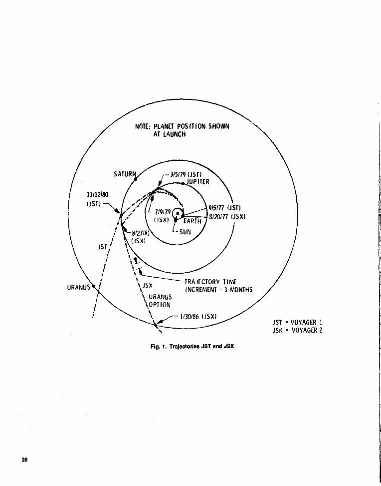
tNf r- 3151791JSr ^t JUPITER
719179 ,915177 (JST)
iJSXI EARTH8!20!77 (JSX)
8127181 SUN(JSX)
$A
11112!80(JST) --
ii
URANUS JSX TRAJECTORY TIMEINCREMENT = 3 MONTHS
URANUS
OPTION
NOTE: PLANET POSITION SHOWNAT LAUNCH
JST
i11
1/30186 (JSX)JST VOYAGER 1JSK • VOYAGER 2
Fig. 1. Trajectories JST and JSX
26

ORIGINAL PAGE Th
OF POOR QUALM ORIGINAL 'PAGE lb
OF POOR QUALITY
EARTH OCCULTATION -_LAUNCH DATE • 915111
SUN OCCULTATION JUPITER TRIVAL DATE • 719179
-+-^, M I SS ON MODULE TRAJECTORYSATELLITE CLOSEST APPROACH
CALL I STO 240, 000 KMGANYMEDE 50, 000 KMEUROPA 190, 000 KM
AA1011R6>,HEA 550, 000 KM
AMALTHE A CRI APIP • 0.5DAYS) EUROPA
(P • 3.55 DAYS)
VYMEDE• 7.1
16 DAYS)
2 HR
CALLI STO(P • 16.69DAYS)
10
(P • 1.77 DAYS)
VIEW NORMAL T0'JUPITER EQUATOR
JST ° VOYAGER 1
Fig. 2. AT Jupiter encounter at 4.9RJ
27

EARTH OCCULTATIONLAUNCH DATE - 8120177
SUN OCCULTATIONJUPITER ARRIVAL DATE - 719!79
MISSION MODULE TRAJECTORYSATELLITE CLOSEST APPROACH
CALL I STO 240, 000 KMGANYMEDE 50, 000 KMEUROPA 190, 000 KMAMALTHEA 550, 000 KM
ERIAPSISAMALTHEAIP - 0.50DAYS) "'
EUROPA(P - 3.55 DAYS)
10(P = 1.77 DAYS)
GAKDAYS)
(P
TO69
VIEW NORMAL TOJUPITER EQUATOR
Fig. 3. Voyager 2 Jupiter encounter at 10RJ
28

LAUNCH DATE • 915177
SATURN ARRIVAL DATE • 11112180
MISSION MODULE TRAJECTORY-- SATELLITE CLOSEST APPROACH
T I N 15,000 KM
T THYS 426, 000 KM
IMAS 96, ODD KM
ENCELADUS 218, 000 KM
D I ONE 148, 000 KM
RHEA 50, 000 KM
PE III A?SIS
SUN DIONE
OCC (P • 2.74 DAYS)
ZONE
EARTH
OCC
ZONE
RHEA
(P - 4.52 DAYS)
ENCELADUS'(P • 1.37 DAYS)
14 NR'rTITAN "' 1
(P • 15.95 DAYS)
TETHYS(P - 1.89 DAYS)
MIMAS
(P • 0.94 DAYS)
VIEW NORMAL TO
SATURN EQUATOR
Fig. 4. Voyager 1 Saturn encounter at URg
29

T IT A 353, 000 KMRH 253, 000 KMT NY S 159, 000 KM
C ELADUS 93,000KMIMAS 34, 000 KM
D IONS 196, 000 KM
DAYSTITAN(P•15.
ENCELADUS(P • 1.37 DAYS)
PERIAPSISEA
4.52 DAYS)DIONE(P • 2.74 DAY
TETHYS(P • 1.89 DAYS)
EARTHOCCZONE
SUNOCC /ZONE
MIMAS(P • 0.94 DAYS)
LAUNCH DATE • 8120177SATURN ARRIVAL DATE - 8127181
F-^ MI SSION MODULE TRAJECTORY- SATELLITE CLOSEST APPROACH
H
V I EW NORMAL TOSATURN EQUATOR
Fig. S. Voyager Saturn encounter at 2.7RS
30

NEAR ENCOUNTER TEST79/10 IA/A o inn JUPITER-SATURN
J - 12 daysJ - l day
^;7—/
/J+10 days
J+15hrs
J - 34 daysJ - 30 days
TRAJECTORY CORRECTIONMANEUVER (TCM)19/11-13)77
HIGH GAIN ANTENNAACQUIRES EARTH— L+95 days
DATES ARE FOR VOYAGER 1
Fig. 6. Voyager 1 mission phases, Earth to Jupiter
w

RADIOISOTOPETHERMOELECTRICGENERATORS (3)
PLANETARY RADIOASTRONOMY ANDPLASMA WAVE ANTENNA
PLASMA
N
COSMIC RAY
EXTENDABLE BOOM
WIDE ANGLE TVi NARROW ANGLE TV/ TV ELECTRONICS
ULTRAVIOLETSPECTROMETER
INFRAREDINTERFEROMETERSPECTROMETERAND RADIOMETER
HIGH—GAINDIRECTIONALANTENNA
MAGNETOMETER (1 OF 43
pf^,5
^s ( Ley
`r
`
\ PHOTOPOLARIMETER
LOW ENERGYCHARGED PARTICLES
THRUSTERS (16)
ELECTRONICCOMPARTMENTS
PLANETARY RADIOASTRONOMY AND SCIENCE INSTRUMENT
PLASMA WAVE ANTENNA
CALIBRATION PANELAND SHUNT RADIATOR
^f
PROPULSIONFUEL TANK
Fig. 7. Voyager spacecraft configuration

^S
c9
1976 1977 1978
A M J J A S O N D J F M A M J J A S O N D J F M AIM
• VIKING -------PRIME
PERIHELION
MISSION Q EXTENDED MISSIONPERIHELION
(EOM
• HELIOS 2 -- ®=^!--------- 0 I ------_PERIHELION
-------------- - _Q^ COMPAT------ --- --- ------ SUBNET LAUNCH
• P 10 VENUS -------------- -------------- -------------- --------- - Q- -- ---- -- -v -------I----- 9---- -----------------------------OVT GDS 0MO
OMPLET• VGIZ ---- ------ ---- -----,-------- m J7 LAUNCHES----- --------
- -----CTA 21 PTM
-- - ---------1-------------- - ------ ^,....,^CTA
21 SC 1 AND 2
------------- CTA 21VE.. DSS 12 DSS-MOOD INTEG TESTS
TWO MONTH DOWNTIME• CTA 21____________ ____ 11111111111
TbNO MONTHS TEST ANDui' ICI
TRAINING AND FLIGHTI I
SUPPORT1• MIL 71---------------------------------------
START OF 5-MONTH DOWNTIME DSS 12• DSS 12___________ ______________ _______________ 1111 11111.________ ------------- FOR S-X CONVERSION 1 JULY 197$__
• DSS 62---------- -------------- -------------- --------- IuIUIII• DSS 44 --------------------------------------------------------- uII IIIIIt
• DSS 14 ----------- --------------------------------------------- -------------- --stt umul
• DSS 42 143------ -------------- ----------------------------------------------------------------------------------------- -------------- -------------- - ^IIInI
• DSS 61 163 ------ ------------- - ----------- -------------- -------------- ^u luau
• DSS 11----------- -------------- i -------------- I -------------- I -------------- I -------------- I ----------------------------- ^m nlllu
Fig. 8. Mark 111-DSN Data Subsystems Implementation Project schedule

DSN Progress Report 42.44
January and February 1978
N75-24216
Viking Extended Mission SupportT. W. Howe
Deep Space Network Operations Section
This report covers the period from 1 November through 31 December 1977. It reportson DSN support of Viking spacecraft activities during the period and continues reportingon the DSN Discrepancy Reporting System, Viking Command support and Trackingsupport. It also continues the reports on the status of Viking DSN klark III DataSubsystem Implementation Project (MDS) related testing.
I. Viking Operations
A. StatusThe two Viking Orbiters continued to make detailed photo
maps of Mars during this reporting period. In addition theymeasured the temperature and water vapor content of theMartian atmosphere. Cloud patterns were checked to see howweather and storms develop. The Orbiters continue to act asrelay stations for Viking Lander data transmission.
Spring equinox occurred in the northern hemisphere ofMars during early November. The frost seen earlier in Landerphotos has disappeared and the polar hood clouds were break-ing up. A record gust of wind of 122 km/h was recorded byLander 2. The Landers continued to take soil samples feranalysis.
The received signal level continued to improve by 0.5 dBmper week because of the shortening distance between Mars andEarth. December telecommunication links had improved to apoint 10 dB stronger than levels recorded one year earlier. TheDecember performance is summarized as follows:
Orbiter link quantity (high-gain antenna) Dec. 1976 Dec. 1977
Uplink AGC, 64-meter, 20 kw, —109 dBm —99 dBmno modulation
Downlink AGC, 64-meter, —143 dBtn —133 dBmsingle subcarrier
X-band downlink AGC, 64-meter —153 dBm —143 dBm
B. Spacecraft Problems
The Viking project declared a spacecraft emergency onNovember 1, when Orbiter 2 indicated a leaking yaw-axis atti-tude control jet. The Deep Space Station in Spain (DSS 62)was brought up to fill a tracking gap between DSS 43 (Austra-lia) and DSS 11 (Goldstone). The leak was stopped by sendingcommands to perform a yaw turn and clear the leaky valve andthen the Reaction Control Assembly (RCA) was commandedoff.
Viking Orbiter 1 (VO . 1) showed a small roll axis gas leak onNovember 18. DSS 62 was released early by the Voyager pro-ject so that data could be obtained to check the gas leak. When
34

data came into lock, telemetry indicated that the leak hadcleared itself. Monitoring continued for the next two days andperformance was normal. It was thought that this particulargas leak was caused by a particle which cleared Itself.
On November 25, VO-I again showed a possible gas leak inthe yaw-axis. DSS 62 was obtained to monitor the data.Analysis determined that the leak indications were not causedby a microleak but were due to a strong and variable gravitygradient torque experienced near periapsis, with Arcturus asthe reference star. The effect was later confirmed using acomputer model.
A problem first noticed during the interplanetary cruisephase of the mission was noted again in mid-October andcontinued sporadically throughout this reporting period. TheViking Orbiwi r highrate data content interferes with the low-rate signal-to-noise ratio. When either Orbiter is in the dualsubcarrier mode at a data rate of 8 kbps or 16 kbps the33.333 bps low-rate SNR is seen to fluctuate by several dB.The effect is most notable during an all zeros data condition.Sidebands of the high-rate channel occur near the 24-kHzlow-rate subcarrier and in some cases are strong enough tocause the stations Subcarrier Demodular Assembly to loselock.
C. ManeuversThere were no propulsive maneuvers during this reporting
period. Nonpropulsive maneuvers continued to occur on bothOrbiters in order to take pictures and to support the BistaticRadar experiment.
D. Radio ScienceRadio Science activities and experimentation continued
during November and December. There were 7 Near Simulta-neous Lander/Orbiter Ranging passes during the period. Grav-ity Field experiment data taking occurred nearly every dayduring the period.
Occultation data was collected during the period exceptduring the times in which there was no DSN coverage, aBistatic Radar pass, Viking Lander Ranging, or a spacecraftroll maneuver.
Viking Orbiter 2 occultations began on November 19 andwill continue through January of 1978.
Differential VLBI coverage occurred on 7 days during theperiod. The Owens Valley Radio Observatory and the Hay-.stack Observatory in Massachusetts supported this experimentusing Viking Orbiter 1 data.
Two new Radio Science experiments began during thisreporting period, The Gravity Wave Experiment, using DSS's14 and 43 and Orbiters I an¢ 2, was.conducted on 12, 14, 23,and 29 December.
This experiment requires six hours of closed-loop two-way,S/X-band doppler, taken at a sample rate of one sample persecond. It also requires simultaneous two station tracking withtwo and three way S/X doppler for one hour taken at the onesample per second rate.
The second new experiment which began during this periodwas Bistatic Radar (BSR). The Bistatic Radar experimentrequires the Viking Orbiter high-gain antenna to be pointed atthe Martian surface, The transmitted signal is reflected off thesurface of Mars and received and recorded on the occultationopen-loop receivers and analog recorders at DSS 14 and/or 43.
There are two types of observations. During a "SpecularReflection" pass the Orbiter high-gain antenna pointing ismaintained for an angle of incidence equal to the angle ofreflection towards Earth. The reflection point scans the sur-face of Mars because of orbital motion. Figure 1 illustrates thegeometry of a Specular Reflection pass. Of primary interestduring these BSR passes are the northern, middle, and polarlatitudes of Mars, which cannot be studied from Earth.
For "Fixed Target" passes, the high-gain antenna is pointedat a fixed location on Mars. Figure 2 shows a Fixed Targetpass, This type of BSR pass will investigate the equatorialregion of Mars to develop information on known sites ofinterest.
Table 1 lists potential Bistatic Radar targets.
Figure 3 shows the station configuration for this experi-ment. The reflected signal contains information about Martiansurface roughness and electrical properties. Similar expert-ments have been conducted using earth based transmitters forradar studies of Mars. Bistatic Radar passes took placebeginning November 8. A total of 10 passes were used duringthis reporting period.
Stations have been able to miintain some closed loopreceiver lock during Bistatic Radar passes. This is believed tobe lock on a sidelobe of the Orbiter high-gain antenna. Al-though the received signal level is relatively weak, at times itincreased to the point at which telemetry lock was achieved.
E. Spacecraft TestsRoutinoy spacecraft testing continued during November and
December,, . Orbiter Command Detector Unit (CDU) signal-to-noise ratt6 estimator (SNORE) tests were conducted on an
35

average of two per week. High-gain antenna calibrations werealso performed.
Viking support. Attempts at corrective action did not improvethe overall situation.
Effective December 7, the routine CDU SNORE checkswere cancelled. Stations were having difficulties setting lowoutput transmitter power levels with the provided calibrationtime. Without accurate settings, the SNORE test results werequestionable. Future tests will be scheduled periodically andappropriate precalibration time provided to insure valid outputpower levels.
11. Network Support
Table 2 shows the Viking Extended Mission (VEM) Track-ing Support for 1977. Noticeable during this period is the factthat December produced more tracking passes than Novemberbut had less tracking hours. This resulted from shorter passesthroughout the network.
Table 3 gives the total number of commands transmitted bythe DSN for the Viking project during 1977. The monthlytotal number of commands has declined since the recordamount transmitted during September of this year. Fewercommands were sent in November than any other month of1977.
Table 4 identifies the DSN VEM Discrepancy Reports gen-erated during the period and 1977. The total number of opendiscrepancy reports has been on the increase since September.
A. Operational Use of Ampex FR-2000A RecordersAmpex FR-2000A analog recorders were installed at each
of the 64-meter DSN stations under engineering change order75.291 early in 1976. These machines were used for playbackof baseband analog data previously recorded on FR-1400 typeof recorders.
Data was available from either Subcarrier DemodularAssembly (SDA) detected data output or from receiverbaseband.
Following the MDS implementation, SDAs at 64-meterstations were reduced from six to four and of these four, onlytwo detected data outputs were recorded on analog tape. Thiscoupled with the requirement to record the third RF carrierwhen more than two spacecrafts were being tracked causedmore reliance on baseband recovery.
By September 1977, the analog baseband record and replaycapability had deteriorated below acceptable operational levelsof performance and impacted the quality of operational
The Viking Tracking and Data Acquisition Manager estab-lished a task team on September 16, 1977 to coordinate thework necessary to reestablish analog baseband record andreplay as a dependable operational capability.
The task team determined that reliable analog record andreplay could be accomplished by:
(1) Recording and replaying data on the FR-2000Arecorders.
(2) Changing track assignments to effect better replaycharacteristics by reducing interference between adja-cent tracks (see Tables 5 and 6).
(3) Recording baseband data only.
The conditions underwhich this capability could be madeavailable for operational use are as follows:
(1) A 5-minute gap in recording every 30 minutes wasrequired to change tapes since only one FR-2000Arecorder had been implemented at each 64-meterstation.
(2) An additional 30 minutes of prepass preparation timewas required to set up the tape machines.
(3) Analog recordings would only be made if the minimumspecified signal-to-noise ratios were met.
(4) A failure of the prime recorder would result in a loss ofanalog data since no backup existed.
Successful demonstrations of the analog baseband recordand replay capability were run with DSS 14 on November 18,and with DSS 43 oil 25. DSS 63 was down for theMDS reconfiguration and no demonstrations were possiblewith this station.
The Viking Project Manager approved this new plan onNovember 22 with the single qualification that the projectmight choose the time at which the recording gaps wouldoccur so as to minimize the loss of critical data.
The FR-2000A recorders were authorized for use for allproject support oil 2, 1977, The Network Opera-tions Plans for each project were revised to show the newanalog recorder configuration.
36

Ill. DSN Mark III Data Subsystem Implemen-tation MDS Testing and Status
Except for DSSs 11, 61, and 63, all stations had completedthe MDS implementation and testing prior to this reporting
period. DSS 61/63 was released from tracking support on
15 October 1977 to begin it's implementation phase. The
'testing phase is scheduled to begin on 1 January 1978. DSS I 1
will begin the MDS upgrade on 15 January 1978.
37

Table 1. Potential 81static•Rader targets
Target
A Chryse Basin
B Utopia
C Apollinares-Mern non iaC site area
H Hellas
PI Plateau
Po Polar regions
T Tharsis
S Soviet landing sites
SM Syrtis Major
Prior radar inferences
Above average dielectric constantand roughness
No data
Variable echoes, generally weak;high diffuse-to-specular ratio
No data
Strong, sharp echoes; averagedielectric constant; unusuallysmooth
No data
Weak, diffuse echoes
No data
Strong echoes; smooth surface
Other information
Large number of surface rocks;Viking 1 site
Large number of surface rocks;Viking 2 site
Low plains with little relief;surface features subdued
Southern basin; few features
Massive (recent?) flows; lowcrater counts
Questions
Basin CharacteristicsAre surface rocks detectable''
Are surface rocks detectable?
Nature of high angle scattering
Basin Characteristics?
Scattering function in very specularregion?
Ice forms, terracing, sculpturing Polar characteristics?
Volcanic ridge and flanks Nature of weak scattering?
Cratered uplands; basin Possible clues to mission failures
Wind-blown surface; variable albedo Basin characteristics?
36

Table 2. VEM tracking support 1677
Jan Feb Mar Apr May Jun Jul Aug Sept Oct Nov Dec 1977Total
DSSTracks'
h
1123 22 10 17 38 40 44 42 26 40 35 42 379
135 142 100 118 228 289 322 343 210 408 310 320 2925
124 1 - 24 17 1 1 1 — — — — 49
11 6 176 119 4 1 7 324
1452 59 SG 20 — — 10 16 28 43 41 45 364
341 392 368 176 46 126 363 329 358 234 2753
4221 25 58 17 17 14 10 — — 14 18 20 214
247 226 453 138 162 112 69 100 116 126 1749
68 62 63 60 57 31 1 24 36 48 45043
721 627—
603 521 486 238
—
O1 141 214 196 3748
44 — _ 7 1 — — 16 26 6 12 — — 68
7 4 99 166 22 51 ^ 349
35 29 12 40 54 51 37 35 38 22 35361
261 227 72 317 461 475 337 322 345 203
— —
3020
2 4 9 3 2 3 S 9 3762 _.,_
7 22 55 14 7
— — —
23 28 36 192
38 28 66 15 23 15 40 64 57 15 36163
327 202 525 78 186 136 399 590 590 136
— —
3169
241 228 207 206 212 180 189 184 156 173 135 164 2275Total
2043 1829 1547 1665 1691 1509 151! 1554 1531 1391 1026 932 18229
'Number of tracks represent the summation of all Viking spacecraft tracked.. Track time, in hours, represents scheduled station support J
pg,IGINAi' pAGE IbOF ppOR QUAIIT`^
39

Table 3. Number of commands transmitted In Viking WendedMission during 1977
USS
Jan Feb Mar Apr May Jun Jul Aug Sept Oct Nov Uec 1977Total
CMUS
11 1,521 1,394 1,027 117 811 -0. 1 795 2,020 3,687 3,064 4,746 19,19112 -0. -0-_ -0. 1,314 7 21 -0- -0- -0- -0- -0- -0- -0- 2,03514 769 1,404 1,206 274_
-0^-0 74 108 2,704 2,108 1,134 1,589 11,370
42 2,072 953 1,778 8 1,619 -0- -0- -0- 18 1,250 -0- 9,58943 919 2,523 -0• 2,094 k1,44 972 1,190 -0- -0- 456 656
_
491 10,74844 -0- -0- 2 1 -0- -0- 5 19 2 -0- -0- 2961 605 1,116 1,328 1,925 3,838 4,257 5,589 5,256 1,371 -0- -0- 27,20762 -0- -0- 1 1,991 -9- 496 -0- -01 -0- -0- 14 5 2,50763 795 472 2,039 381 675 383 2,579_ 2,318 1,610 847 U -0- 12,099
Total 6,681 7,862 7,381 _ 8,105 7,462 7, 308 8,101 8,815 11,617 8,489 6,118 6,831 94,770
40

Table 4. 08N VEM dlscrepaney reports
Jan Feb Mar Apr May ¢ Jun Jul Aug Sett Oct Nov Dec
DSSQaCb
1 t 2 t4 3 4 1 2 2 2 !11 0 4 6 3 3 6 7 7 1 3 2 4
4 0 0 5 7 0 0 Q 0 0 Q 112 0 0 0 2 5 7 Q 0 0 0 Q 0
14 11 4 3 2 0 6 4 5 10 14 714
2 19 33 9 2 2 2 18 14 24 13 16
q 2_ 0
0 U 0 0 0 0 1 3 342 1 3 7 2 0 0 0 0 0 0 2 3
10 11 U 4 B 2 1 0 Q 0 3 114313 10 12 1! 17 14 6 1 0 5 7 14
0 0 0 q 0 0 1 I 0 0 0 044 0 0 2 1 0 0 0 4 l 0 0 0
l l 0 0 1 U l 0 0 0 0 061 9 6 3 1 2 6 4 7 4 4_ 0 0
0 0 1 2 0 P 0 0 02.
0^°' 262 0 8 2 1 2 1 0 0 0 0 2 0
1 7 1 0 4 3 4 9 8 4 I 063 4 3 18 6 4 12 4 17 17 7 5 1
Others,4 3 2 4 7 10 8 5 7 10 13 13
3 a 10 7 l2 !3 ^ 16 9 8 l5 21 13
12 24 31 17 23 20 21 28 36 39Total 32
38M38^^62 93 43 47 61 39. 63 45_ _ __58 —A2 51
30 = Number remaining open at end of month.
bC = Number closed during rnomli.
,Other = DSN, NDPA, NOCA, GCF.
41
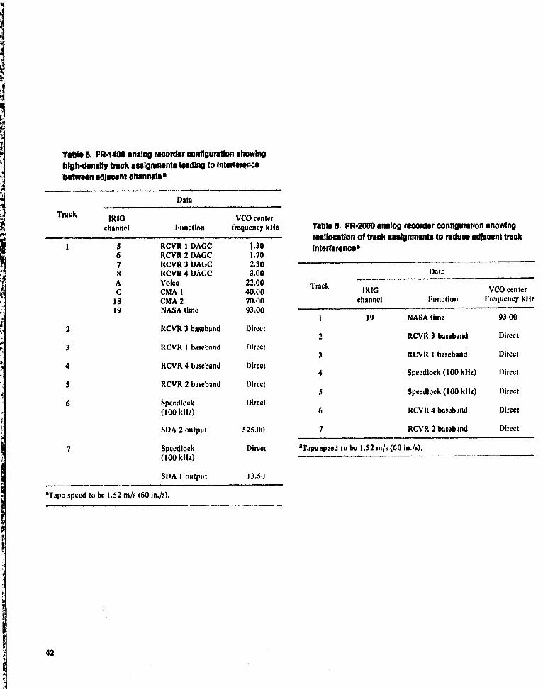
Table 6. FR•1400 analog recorder configuration showinghlgh4onsity track assignments loading to Interferencebetween adjacent channels
Data
Track TRIG VCO centerchannel Function frequency kHz
1 5 RCVR 1 DAGC 1.306 RCVR 2 DAGC 1.707 RCVR 3 DAGC 2.30S RCVR 4 DAGC 3.00A Voice 22.00C CMA 1 40.00is CMA 2 70.0019 NASA time 93,00
2 RCVR 3 baseband Direct
3 RCVR 1 baseband Direct
4 RCVR 4 baseband Direct
5 RCVR 2 baseband Direct
6 Speedlock Direct(100 kHz)
SDA 2 output 525.00
7 Speedlock Direct(100 kHz)
SDA 1 output 13.50
°Tape speed to be 1.52 m/s (60 In./s),
Table d. FR•2000 analog recorder configuration showingreallocation of track assignments to reduce adjacent trackInterference•
Date
Track TRIG VCO centerchannel Function Frequency kHz
1 19 NASA time 93.00
2 RCVR 3 baseband Direct
3 RCVR l baseband Direct
4 Speedlock (100 kHz) Direct
5 Speedlock (100 kHz) Direct
6 RCVR 4 ba€eband Direct
7 RCVR 2 baseband Direct
°Tape speed to be 1.52 m/s (60 in./s),
42

VIKING ORfITER
VIKING OtuITER
Fig. f. Specular reflection pass Fig. 2. Fixed target pass
TOEARTH
TO EARTH
ORIGINAL PAGE lbOF POUR QUALITY
5 OLR CH I PPRr— S
SYNTH TONE
LO E
SPD TWM S — J
,..- RCPS-X S-S
SPDSYNTH 1 VGO
CONE 5ITCHLCP ASSY
_ 5-MHz REF(^G)
Ki
MULLT S0-MHa REF (CRG)
S -X S-S SYNTH 2 VCO
iCONEI
XROX
iTWMI £
ILO
TONE5 SYNTH
FR-1400
AODR
L_— OLR CH 2X S-X SIGNAL
X r----1 r----I
S XLTR 2 S XMTR ^^ SYNTH_a^°^-----I I------I -- 4--^
Fig. 3. Sistatic Radar DSN station configuration
43

DSN Progress Report 42.44
January and February 1978
N78= 2421'
Pioneer Mission SupportT. P. Adamski
DSN Operations Section
This article reports on activities within the Deep Space Network in support of tirePioneer Project's in flight spacecraft during the period August I P 7 7 through January1978, The amount of tracking coverage provided by the NetwoM and a summary ofoperational testing of the Mark III Data Subsystems at DSSs 42143 and 61163 arepresented,
I. Pioneers 6, 71 89 and 9As indicated by Table 1, coverage of these spacecraft has
decreased from 'the levels of the last reporting period (Ref. 1),A total of 26 tracks were conducted during August, primarily'for the acquisition of radio metric data to be used for trajec-tory updating. In the following months, coverage was minimaldue principally to increased Network loading in support ofhigher priority users. Tracks in the months 'subsequent toAugust were used primarily to verify Mark III Data Subsystem(MDS) performance at the Deep Space Stations.
All of these spacecraft celebrated launch anniversaries dur-ing this reporting period. Pioneer 7 was eleven years old on 17August, Pioneer 9 was nine years old on 8 November, Pioneer8 was ten years old on 13 December, and Pioneer 6 was twelveyears old on 16 December. In general, all four spacecraft havecontinued operating normally. The principal exception wasPioneer 8 which experienced a severe degradation in one of itssun sensors. The extent of the degradation will not be knownuntil the spacecraft reaches perihelion when the sensor may beable to detect the sun.
The degraded sensor provided the spacecraft roll referenceand sun pulse. Without the sun pulse, most scientific data areuseless as the instruments have no pointing information withwhich to correlate their measurements. As a consequence, allinstruments have been powered down; the plasma analyzer willbe turned on whenever the spacecraft is tracked since datamay be recovered from this instrument even in the absence ofthe sun pulse.
II. Pioneers 10 and 11Pioneer 10 continues to operate satisfactorily. The space-
craft is now almost 15 astronomical units (AU) from the earthand the round trip light time is over four hours. Trackingcoverage has remained fairly constant since the last report.Coverage by the 26-metre stations has declined sharply as thespacecraft is approaching threshold for those facilities. Track-ing coverage for the last six months is tabulated in Table 1 andcoverage for the last twelve months is shown graphically inFig. 1
44

Pioneer I Is also operating nominally. Earth-spacecraftrange is now approximately 5.5 AU and the round-trip lighttime is over one and one-half hours. Tracking coverage isshown in Table I and Fig. 2 for the past six months and twelvemonths, respectively.
On 3 August, the spacecraft passed througli its fourthsuperior conjunction at a minimum earth-Sun-probe angle of9°05 (approximately 33.3 Ro). No significant telemetry degra-dation was observed at this great an angular separation. Someincrease in Doppler noise was experienced, as shown in Fig. 3,but this enhancement was somewhat less than that expected.
The plagma analyzer on Pioneer 11, which ceased operationin April 1975, began to output data again on 4 December.Since that date, the instrument has responded to groundcommands and appears to be fully operational. This experi-ment should provide much valuable data during the Saturnencounter in September 1979.
A Saturn targeting maneuver, scheduled for late January,has been delayed until mid-year in order to decrease theamount the spacecraft must be turned off earth-pointing.Current plans are for Saturn periapsis to occur outside thevisible rings, but an option remains for a passage between theplanet and its rings.
Ili. Mark III Data Subsystems Supportof Pioneer
Since the previous report, Mark Ill Data Subsystem (MDS)verification testing for Pioneers 6 through I1 has been com-pleted at DSSs 42/43 and 61/63. A total of nine demonstra-tion tracks of the Pioneer spacecraft were conducted at DSS42/43 between the date the station was returned to service (26September) and the date of configuration control application(18 October). DSS 61/63 participated in 21 Pioneer demon-stration passes during the period 3 January (return to service)and 31 January (configuration control application).
No significant, MDS-related anomalies were experiencedthroughout either period of verification testing. The majorityof the minor anomalies encountered were related to operatortraining and familiarization. These problems decreased as oper-ations personnel became more proficient, and more knowledge-able of the new systems.
DSS 11 is currently undergoing upgrading to an MDS con-figuration. Verification testing of this station will begin inMarch and will follow the same pattern of demonstrationpasses as was used for the other stations of the Network. Afuture article will report on this testing.
Reference
1. Adamski, 1. P., "Pioneer Mission Support," in The Deep Space Network ProgressReport 4241, pp. 33-38, Jet Propulsion Laboratory, Pasadena, Calif., October 15,1977.
45

Table 1. Pioneer tracking coverage
'TrackingMonth Spacecraft Station Tracks Time,hype
hr:min
August Pioneer 6 26 in 36:00Pioneer 7 26 in 69:56Pioneer 9 26 in 8 42:41Pioneer 10 26 ra 1 4:35
64 in 195:07Pioneer 11 26 in 527:38
_64 in 6:28
September Pioneer 10 26 in 2 11:1264 in 29 225:50
Pioneer 11 26 in 396:5664 in 14:00
October Pioneer 7 26 in 4 18:21Pioneer 8 64 in 3:37Pioneer 10 26 in 4:35
64 in 237:37Pioneer 11 26 in 315:51
64 in 59:01
November Pioneer 10 64 in 265:57Pioneer 11 26 in 364:06
64 in 16:03
December Pioneer 10 26 in 1 0:5064 m 40 267:53
Pioneer 11 26 in 36 289:0964 in 28:33
January Pioneer 6 26 in 7:40Pioneer 8 64 in 6:18Pioneer 9 26 in 1 5:34Pioneer 10 64 in 223:58Pioneer 11 26 in 50 341:38
64 in 11:11
ORIGINAL PAGE ISOF POOR QUALITY
46
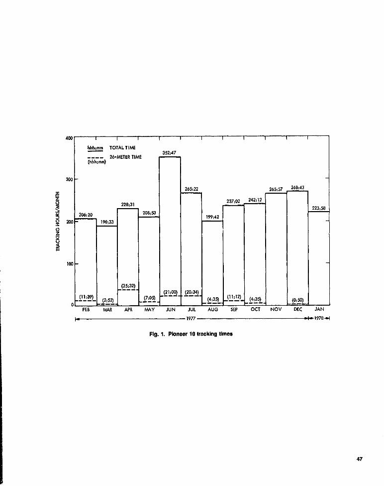
400
300
x
O 200sOZYU
A
100
0
TTT_hhh:mm TOTAL TIME
_ 26-METER TIME352:47
(hhh:mm)
265:22 265:57 268:43
217:02 242:12228:31
223;58
206:20
190;33
208153199:42
(35:32)- ^ - (21_00) (20:34)
(11:39) (2:52) (7:05) _ _(4,35) (11:12) (4:35) L (0:50)
FEB MAR APR MAY JUN JUL AUG SEP OCT NOV DEC JAN
1977 -`- 1978+{
Fig. 1. Pioneer 10 tracking times
47

goo
700
600
p
500
= 400
U' 356:40Z
u300
200
100
694:32687:33
673:06649:23
544:58 534:06
hhh:mm TOTAL TIME
64-METER TIME(hhh:mm)
410:56
7 374:523,. 80:09
317:42
352:49 1
38:13 ^^
- - -(23:54) - - )
- - (27:28) (180^ (6:28)
(14:00) (16:03) (28,31).j (11:11)
0 _ - -FER MAR APR MAY JUN JUL AUG SEP OCT NOV DEC JAN
1977 1978 +I
Fig. 2. Pioneer 11 tracking times
48

0.100
N
W_N
Z 0.010
6C6CL.
8
0.003
#EXPECTEDNOISE
0• r • .•
• • . M•
•0 .• .• ^•• •^ ••• .•
r • • '.• • 0
1MINIMUMSEPARATION
•• • r r • r
•^ • r
0.001160 180 210 230 250
270
DAY OF YEAR
Fig. 3. Doppler noise during Pioneer 11 superior conjunction
49

DSN Progress Report 42.44 January and February 1978
N78-24218
Helios Mission SupportP. S. Goodwin
TDA Mission Support Office
W. N. Jensen and G. M. RockwellDSN Operations Section
This article reports on activities of the DSN Network Operations Organization insupport of lire Helios Project from 15 December 1977 through 15 February 1978.
I.Introduction
This article is the twentieth in a continuing series of reportsthat discuss Deep Space Network support of Helios MissionOperations. Included in this article is information on Mark IIIData Subsystems (MDS) testing at the conjoint Deep SpaceStation 61/63 (Madrid, Spain) and other mission-relatedactivities.
II.Mission Operations and Status
The Helios-1 spacecraft experienced an anomaly over DSS43 (Canberra, Australia) on January 2, 1978. DSS 43 lost thedownlink, and at first the station suspected a maser problembut after investigating this possibility all station systemschecked normal. DSS 44 (Honeysuckle Creek, Australia) wasthen asked to track the spacecraft, but no signal was observed.The spacecraft was then blind-commanded to its original con-figuration and carrier lock was achieved on DSS 43's receiver,but no telemetry data lock was obtained. Additional com-mands were transmitted to configure the spacecraft to 512 bitsper second (bps) coded telemetry in Format 4. At 04:34UTC, DSS 43 reported data lock. The reason for the anomalywas subsequently traced to a spacecraft regulator switch caus-
so
ing a power drop, which knocked the high-gain antenna offpoint resulting in a loss of downlink signal. Later, the data ratewas changed to 256 ups to improve the signal-to-noise ratio(SNR).
On January 24, 1978, at 04:16 UTC, Helios-2 passedthrough its sixth aphelion with no scheduled ground stationsupport. Last support prior to aphelion was over DSS 12(Goldstone, California), which had LOS at 21:05 UTC on 23January. The next support after aphelion was over DSS 67(Germany). The spacecraft was in a medium power mode andonly Experiments E-5A, E-5C and E-8 were on.
On January 15, 1978, DSS 42 (Canberra, Australia) lostHelios-2's downlink due to lunar occultation. Because thepredicts did not show this event occurring, 1.4 hours of datawere lost which could have been stored on board the space-craft for future recovery. As a result, the appropriate partieshave been notified and hopefully this type of oversight willnot occur in the future.
A special Helios-2 de-spin maneuver over DSS 42 was con-ducted on January 16, 1978. Two attempts were requiredbecause the spacecraft's power regulator No. 1 switched on thefirst attempt, causing a maneuver abort.
ORIGINAL PAGE IbOF POOR. QUALITY

On January 27, 1978, the Hellos-2 spacecraft pessedthrough Its fourth aphelion. Ground station coverage wasprovided by DSS 42 (Canberra, Australia). The spacecraft wasconfigured in medium power mode with all experiments on,except for E-3 and E-9. Overall coverage of both Helios-1 andHelios-2 for this perind is listed in Table 1.
III. Special ActivitiesA. DSN Mark III Data Subsystems (MDS) Update
As reported earlier (Ref. 1), DSS 61/63 (Madrid, Spain)began MDS implementation on October 16, 1977. The Com-plex began its test and training phase on January 1, 1978. TheHelios training consisted of demonstration tracks being con-ducted with DSS 61 (the 26-meter side) and DSS 63 (the64-meter side). The first demonstration track was successfullyperformed on January 14, 1978. A total of six demonstrationtracks were performed with DSS 61/63 with no majordifficulty.
The DSS 61/63 Complex was placed under configurationcontrol to support all flight projects on January 31, 1978.
On January 15, 1978, DSS I I (Goldstone, California) wasdeactivated for MDS implementation; This Is the last DSNfacility to undergo modification and will complete the net.work's MDS upgrade. The MDS configuration for DSS 11 Isshown in Figure 1. A report on DSS I 1 will appear in die nextarticle.
B. Support of On- 9oard and Ground ExperimentsIn the last article, it was hoped that some results of the
Experiment 12 (Faraday Rotation) data analysis would beavailable for this article, but this is not the case. As of thistime, no data have been released for publication. As was statedbefore, due to the large amount of data collected, processing istaking longer than expected. As soon as results become avail-able, they will be summarized In the next sequential article.
Reference
1. Goodwin, P. S., Rockwell, G. M., "Helios Mission Support", in The Deep SpaceNetwork Progress Report 42-43, pp. 2446, Jet Propulsion Laboratory, Pasadena,California, December 15, 1977.
51
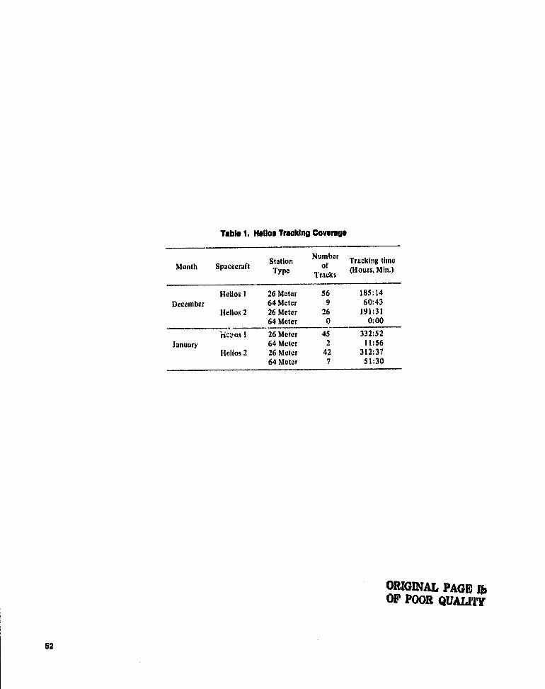
Table 1. Hellos Tracking Coverage
Month Spacecraft StationType
Number
ofTracks
Tracking time(Hours, Min.)
Helios 1 26 Motor 56 185:14Deembet 64 Meter 9 60:43
Helios 2 26 Meter 26 191:3164 Meter _0 0:00
i{c;los 1 _ 26 Meter 45January 64 Meter 2 11:56
Helios 2 26 Meter 42 312:3764 Meter 7 51:30
ORIGINAL PAGE fibOF POOR QUALI'T'Y
52
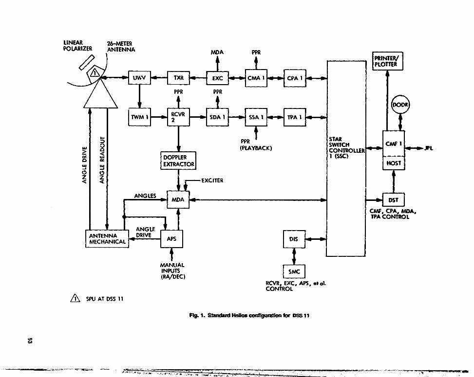
LINEAR 2$-METERPOLARIZER ANTENNA WA PPR
L'1 UYr'V TXR EXC CMA 1 CPA 1
PPR PPR
TWM 1 2CVR SDA 1 SSA I TPA 1
PPR> Q(PLAYBACK)
c DOPPLERW W EXTRACTORJ J
Q Q r -- EXCITER
PRINTER,/PLOTTER
STARSWITCHCONTRI1 (SSC)
CAW 1JPL
HOST
MDA1-J
CW, CPA, MDA,TPA CONTROL
1 • ANGLEANTENNA DRIVE APSMECHANICAL
MANUALINPUTS(WDEC)
/1 SPU AT DSS 11
DIS
SMC
RCVR, EXIC, APS, et alCONTROL
Fig. 1. Sbwxl rd Hm3w congguraftn for am 11
ca
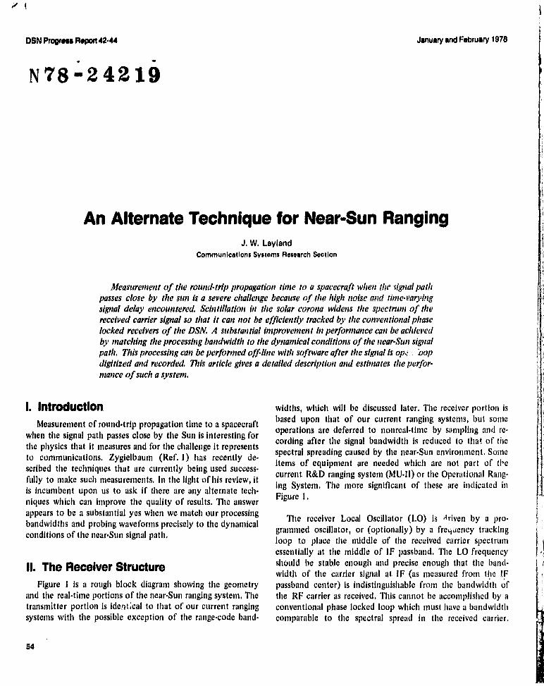
W t
DSN Progreas Report 42.44
January and February 1878
N78-24219
An Alternate Technique for Near-Sun RangingJ. W. Layland
Communications Systems Research Section
Measurement of the round-trip propagation time to a spacecraft when the ;signal pathpasses close by the sun Is a severe challenge because of the high noise and time-varyingsignal delay encountered. Scintillation in the solar corona ►videns the spectriorn of thereceived carrier signal so that it can not be efficiently tracked by the conventional phaselocked receivers of the USN, A substantial Improvement hi performance can be achievedby matching tire processing bandwidth to the dynamical conditions of the gear-Sun signalpath, 77ds processing can be performed off-line with software after the signal is op,, 1 'Oop
digitized and recorded. 77ds article gives a detailed description and estimates tine perfor-mance of such a system.
1. Introduction
Measurement of round-trip propagation time to a spacecraftwhen the signal path passes close by the Sun is Interesting forthe physics that it measures and for the challenge it representsto communications. Zygielbaurn (Ref. 1) has recently de-scribed the techniques that are currently being used success-fully to make such measurements. In the light of his review, itis incumbent upon us to ask if there are any alternate tech-niques which can improve the quality of results. The answerappears to be a substantial yes when we match our processingbandwidths and probing waveforms precisely to the dynamicalconditions of the near-Sun signal path,
11. The Receiver Structure
Figure 1 is a rough block diagram showing the geometryand the real-time portions of the near-Sun ranging system, Thetransmitter portion is ider)Gcal to that of our current rangingsystems with the possible exception of the range-code band-
widths, which will be discussed later. The receiver portion isbased upon that of our current ranging systems, but someoperations are deferred to nonrcal-time by siimpling and re-cording after the signal bandwidth is reduced to that of thespectral spreading caused by the near-Sun environment. Sonicitems of equipment are needed which are not part of thecurrent R&D ranging system (MU-11) or the Operational Rang-ing System. The more significant of these are indicated inFigure 1.
The receiver Local Oscillator (LO) is given by a pro-grammed oscillator, or (optionally) by a frequency trackingloop to place the middle of the received carrier spectrumessentially at the middle of IF passband. The LO frequencyshould be stable enough and precise enough that the band-width of the carrier signal at IF (as measured from the IFpassband center) is indistinguishable from the bandwidth ofthe RF carrier as received. This cannot be accomplished by aconventional phase locked loop which must have a bandwidthcomparable to the spectral spread in the received carrier.
54

Extraction of the carrier reference phase for coherent detec-tion of the range-code sidebands can be performer s in a near-optimal manner from the recorded quadrature samples of thecarrier signal,
r(t) = n(t) + a sin {cae [t - 1101
(1)
+ tit Cos (wm [: - 1A01 + 0m) + 0, 11`j
The receiver coder is not rate-aided by the estimate of itsdoppler frequency in real time, so that once synchronized withthe transmitter, it remains so throughout the tracking opera-tiort. The range-code doppler should in all cases be much lessthan the spread-carrier bandwidth, so that correction for therange-code doppler can be applied without loss to the recordedquadrature samples of the detected range code.
We expect two principal benefits with the nonreal-timeprocessing: (1) the carrier phase reference for the i th samplecan be extracted from an optimally weighted sum of the jthcarrier samples for all j in the range i - k < j < i + k, where theweighting values, and the memory-limit k depend upon theautocorrelation function (hence bandwidth) of the receivedcarrier phase. Since this carrier reference is constructed usingthe jth samples for j > i, as well as for j < i, there is potentiallya 3-dB improvement in the SNR of this phase reference rela-tive to an ideally meched phase-locked loop which mustdepend only upon signal received prior to the sample ofinterest, i.e., for j <i only. In addition, the nonreal-time phasereference need not suffer the 1-dB limiter suppression factorpresent in the DSN tracking loops. While such small factorswoi ►ld not be important if the phase-reference had high SNR,they add directly to data SNR whe y. the phase reference hasbelow unity SNR.
(2) The phase of the range coders can be completelyaccounted for throughout the tracking pass. This means that ifit is necessary, data from the entire pass can be accumulated toprovide one range acquisition, rather than depending upon acomplete short acquisition falling wWL'n favorable signal con-ditions. DRVID can be obtained by postprocessing wheneverthe signal is strong enough for the doppler data to be valid,and strong enough for the received range code phase to betracked as a function of time.
Without the rate-aiding of the range coders from dopplerdata, the bandwidth of the range code used need only be setlow enough to accommodate changes in group delay whichresult from charged particle density changes. Were rate-aidingby doppler to be used, the allowed range code bandwidthwould be reduced by 1/2 to accommodate changes in thedifference between group delay and phase delay.
M. Nonreal-Time ProcessingThe equations which follow describe the nonreal-time pro-
cessing. Let the signal as received at the antenna be r(t):
In Equation (1), n(t) is additive noise, a is signal amplitude,W. is carrier frequency, n(t) is the time-varying phase delay, ntis the range-code modulation index, wm is the range-codefre ;uoncy, 77'(t) Is the time varying group delay, and ¢,,, and0, are arbitrary phase-shifts on modulation and carrier. Let thecode-reference waveforms be unit power sinusoids: f{sin/cos } (Cim t); and let the carrier-reference waveforms beunit power sinusoids: %ff {sin/cos}(w,t). With no code rate-aiding, Wm will differ frorr, wm primarily by tite doppler onW,,; ca, should differ from w, by the error in predicting(tracking) carrier doppler.
Only the difference-frequency terms of the cross productsbetween r(t) and the reference signals will be consideredbecause sum-frequency terms are filtered out in processing.The low-frequency terms which appear integrated at points aand b of Figure I are
In: (t)cos (m) {cos1QWC -
w^j t - w0 r?(t) + 4^C) + n c(t)s
(2)
The low-frequency terms which appear integrated at points cthrough f of Figure 1 are
2 sin (m) ^ tin I([wnr - C` I t - wm t7 , (t) +gym)
X {sin j ([wc - c j t - wcrl(t) + 0,) (3)
+ 11CCW or I 11SC(t)lnes(t) rrSS(t)
The factor t is the amplitude of the sine-wave fundamental ofa squarewave. If n(t) can be assumed to be white and Gaussianwith spectral dens: i No, the six noise terms in Equations (2)and (3) are also white, Gaussian, and independent, with den-sity No . By earlier assumption, the bandwidths of the signalterms in Equations (2) and (3) are the same as the bandwidth
ORIGINAL PAGE 1b 55
OF POOR QUALITY
of the spread -carrier. These signals are integrated (or low-passfiltered) suitably for that bandwidth and then sampled andrecorded for final processing later.
Information about the sequence {q'ct } can be convenientlydestroyed by taking cross products of the Rs.
If the one -sided half-power bandwidth of the carrier spec-trum is 120 Hz, we should be able to recover virtually all ofthe signal power by fltering each of the six signals to 250 Hzand sampling at 500 Hz. Since these signals are composedpredominantly of Gaussian noise, quantization to 8 bits foreach sample is more than adequate. This yields a recording rateof about 25 kb/s, so that a standard 730-m (2400-ft) reel ofmagnetic tape could record in excess of an hour of data. Thisrecord rate could probably be cut by a factor of four, throughcoarser quantization or narrow filtering, with only minordegradation.
For simplicity of exposition in what follows, the sampledsignals will be assumed to be Nyquist -rate samples of bothnoise and signal processes. Modifications necessary to accountfor the actual spectrum of the carrier are straight-forward andnot discussed. Let Ycj = [wc - 4:j tj - wcrt (tj) + 0, be thecarrier phase at time tj , *,,, j = [wm - 6.. J tj - wn,n (tj) + 0mbe the range -code phase at time tj , and denote the variousnoises at time tj by nx j = nx(tj) where x ranges over thevarious noise subscripts in Equations (2) and (3). The sequence{*m j } contains the desired range information. The sequence{4r,j } contains little or no useful information because of thefluctuations in rr(t). The six samples at time tj (subscript tassumed) are
Rr _ k cos (m) sin (* c) + rr
Rts = cos (m) cos (*c) + nra
Rcc = 2 sin (m) t cos (TM ) cos (T c) + nce
(4)
PCs = 2
sin (m) t cos (*m ) sin (41c) + ncs
Rsc = 2 s^ .n (m) t sin (xVm ) cos (4r c) + nsc
RSS = 2 sin (m) t sin (gym ) sin (41c) + nss
'C PCC • PIS + PIS • Pic
RS = Rao ' R ta + Qss ' P o
Taking expected values,
a2 t sin (m) cos (m) cos (gym)
2NF2
22 - t sin (m) cos (m) sin (gym)
and if V denotes 02 > for any of the noise terms,
2Variance 0' } = 2 • V2 + V •
4 t2 sin (m) cost m )
2V • 2 cost (In)
(7)2
Variance {{is } = 2 • V2 + V • 4 t2 sin (m) sin (`l'm )
2+ V • 2 cost (M)
The 0, Rs cross products are accumulated for as long asthe variations in 41 m will permit in order to estimate the rangeinformation which is in q1m • The amplitude SNR of R, is
a cos (m) , a sin (m) t cos (XPm )2V 4V
P,
2 + (a cos (rn))2 + (a sin (m) i;)2 cos2 (^Y )2V 4V m
(8)
while that for ps is similar. If the carrier signal is strongrelative to the noise, and the modulation index m is small,then p'c converges to
(5)
(6)
56

1.5 p 3.5
B -- 2 (TP—O) +0.25 (10 (15)
(13)
• cos (q M ) if a «\/—V
p^ sin (m) • •cos (gym ) if a cos (m) »
(9)
This result is identical to the comparable result for coherentdetection when a strong carrier is tracked by a phase lockedloop. If the total signal is weak relative to the noise, then p'" isapproximately
zp'C z ( 2^ • cos (m) • sin (m)
(10)- t • cos (IV.) if a «-V/—V
When a conventional phase locked loop tracks T jt), theloop SNR, RL should be given by
R = r1
cf2 c^^ (fn)L
(11)
Where r] is a correction factor for the relative bandwidths ofthe tracking loop and the samples to be recorded (cf. Eq. (4)).By the bandwidth assumptions, n < 1. The information on cos(,R„ ^) is now contained in P,,, which has expected value
2 sin (in) t cos (^,n ) r/ I (RL )l1o (RL )^ (12)
The modified Bessel functions Ii(-) derive from the trackingerror of a first-order phase locked loop following T jt). Theweak-signal asymptote for the amplitude SNR of R,o is;
3P —_ (2^= • n • sin (in) • i; • cos' (rn)cc
)
IV. Ranging Link Design
Using the receiver structure described above, ranging linkdesign is completed by specifying the bandwidth within whichthe signal must be measured to ensure reliable operation, andfrom this and the spectral broadening information, the band-width of the range code itself. Data from previous solar con-junctions will be used as a guide.
The three primary degradati^ : . t, s are shown approxi-mated in Figure 2 as a function of p R/R Q , the distancefrom the Sun of the signal ray path at its closest approach,given in units of the solar radius. The approximations shownare slight overestimates to actual data for p > 1.7. They are ofdubious value for p < 13 where no data was found.
The receiver system temperature increases drastically as theantenna beam approaches the Sun's disk. Rockwell (Ref. 2)developed an approximation to the system temperature in-crease caused by close approach to the Sun which is
TSUN ^5.6exp (16.3/(p+1))
when written in terms of p. His approximation is convenientlyoverestimated by
T1x 20 • (L)_r.
s + 3 • ( 10) 4 (14)SUN
This form is convenient for graphic display and "calculation"since it is representable as the sum of straight line segments ona log-log plot. In Figure 2, the asymptotes are shown for
TsUN in dB degradation relative to a nominal system tempera-ture of 20 K.
Spectral spreading data has been presented by Woo(Ref. 3). This data is for one-way transmission at S-band witha variety of spacecraft, and a variety of p. The carrier spectrumis spread by scintillation into an almost Gaussian shape. Thehalf-power bandwidth of this spread carrier is slightly over-estimated by the function
which may be very much less than p, for small a. Thenonreal-time processing should thus perform much better thanreal-time coherent detection when the signal is weak, and atleast as well when the carrier signal is strong.
This form is again chosen for graphic convenience. In Fig-ure 2, B is shown in dB relative to 1 Hz.
Angular broadening of the ray-path from the Helios 1 space-craft was inferred by Woo (Ref. 3) at p = 1.7. Assume that this
57
measurement is consistent with prior determinations at muchlarger p, at a similar "quiet" Sun condition. Then the factor bywhich the beam cross-section of the DSN 64-m antenna isexceeded is approximately
Beam Overspread x 10 3 X p-' 9 + 1 (lb)
when a 'moderate' solar activity is assumed. The S-band signalpower loss due to this beam spreading is shown in dB inFigure 2.
Amplitude scintillations can also cause severe short-terndegradation. However, most available literature seems to implythat tt ►e overall long-term effect call almost negligible, so itis tentatively ignored here.
For the ranging link calculations, the bandwidths of thespread spectrum of the range code is proportional to that ofthe carrier on which it resides, but reduced by the ratio of therange code frequency to tine carrier frequency. For two-wayS-band transmission, the spectral spreading should be f timesthat for one-way S-band transmission.
For two-way S-band up/X-band down transmission, thespectral broadening takes place almost entirely on the S-bandtnplink. The received X-band carrier bandwidth will be 11/3times that of the one-way S-band link as a result of themultiplication to the S-band frequency in the transponder.The range-code bandwidth will be essentially the same as forthe one-way S-band link. The angular beam-spreading loss,which pertains to the down-link only, is reduced for X-band to(3/11)2 times its S-band value.
An example link calculation has been carried out usingpower assumptions pertinent to the recent past Viking solarsuperior conjunction. Then, the undegraded down-link carrierpower was approximately -143 dBm, and the ranging sidebandpower was approximately -153 dBm. These ranging sidebandsconsist mostly of a turned-around copy of the uplink rangecode whenever the S-band uplink is suitably strong relative '-)thermal noise at the spacecraft. Using these parameters, and a"strong uplink" assumption, the ranging link SNR is as shownin Figure 3 as a function of p for a two-way S-band link. Onlythe straight line asymptotes are shown, The ranging sidebandpower-to-noise density ratio (P,/N,) is shown in dB-Hz. Whenthe solar impact parameter p is moderately large (p > 10), thisratio is approximately the same as it is far from the Sun. As pdecreases below 10, the increased system temperature andbeam-spreading losses cause severe degradation. The carriersample SNR (P,INe-Ws) is shown in dB. The sample band-width is the two-way counterpart of the half-power bandwidthdisplayed in Figure 2, so that there is a 3-dB direct signal
power loss incurred. As p decreases, the increase in samplebandwidth joins with increased system temperature and beamspreading losses to degrade the SNR as shown. The detectedP,/No is that to be obtained through the quasi-coherentscheme described above, as represented by Eq. (8).
A ranging measurement SNR of +20 dB can be achieved atp x 1.85 by filtering this measurement to 10- 2 Hz if signifi-cant power is not to be lost. From Figure 2, the half-power bandwidth of the S-band (2.3 X 10⁹ Hz) carrier at p = :.85 is19.5 dB-Hz one-way (21 dB-Hz two-way). This spectral spreadon a range code of 10 5 Hz or less will fit within a 10- 2 I•Izmeasurement bandwidth. For an S-band uplink/X-band down-link, the ranging link is as shown in Figure 4, as a function ofp. This link appears to be operable at a somewhat smaller valueof p than the two-way S-band link because the carrier band-width expansion due to frequency multiplication to X-band ismore than counterbalanced by the lessened degradation of theX-band downlink.
The value of p for which ranging appears to become un-workable is in tite vicinity of 1.8 to 1.9 with the assumptionsused. Tine actual value will vary from this depending upon theactivity level of the Sun, and tine validity of the variousassumptions and approximations. In particular, the assumed"strong" uplink is probably also degrading as p decreases, andthis degradation would be reflected in a reduced P,/No in thedownlink. This effect needs to be examined, but should notdramatically change the threshold value for p.
For conventional phase locked loop carrier tracking andcoherent detection, and the assumptions of Figure 3 and Fig-ure 4, the value of p for which ranging appears to becomeunworkable is in the vicinity of 2.0 for both S/S and S/Xranging links. In fact, the closest range point achieved to datewas at p = 2.0 (< SEP = 0.55 °) using the conventional DSNreceiving equipment in conjunction with the Mu-it rangingsystem (Ref. 1).
V. Signaling StrategyIn practice, only a part of the ranging siVial energy can be
placed into the highest frequency code to be used. Theremainder must be transmitted as lower frequency tones inorder to resolve ambiguities in the measured range 'to at leastthe a priori uncertainty in that measurement. Suppose thatoverall one half of the signal energy is to be allocated to thehighest frequency code for which spectral spreading is withinthe measurement bandwidth, and the other half allocated to
58

resolving ambiguities. This can be achieved conveniently in asequential component system by dividing time into equal-length segments, e.g. 30 sec, and using every other segment forthe high frequency code component. A signal received inseveral segments can be combined together as allowed byspectral spreading of that code component, and as neededfrom SNR considerations.
The remaining segments should be allocated to lower fre-quency range code components such that the entire measure-ment strategy is robust in the face of larger-than-expectedvariations in the plasma delay, and such that the a prioriambiguities can be resolved reliably. Let C, denote the highestfrequency code component, and let C, be assigned to alleven-numbered time segments. Two feasible signalling strate-gies for the odd-numbered segments are as shown in Table 1,under the assumption that ambiguity can be resolved withonly five code components. Note that at no time is a code"chopped" by a higher frequency code. The linear strategy isanalogous to an acquisition as performed by current rangingsystems, while the logarithmic strategy should be somewhatmore tolerant of unexpected delay variations.
A DiscussionFrom the information in the preceding sections, it is clear
that we can Improve the performance of near-Sun rangingoperations by quasi-optimal dote; Lion techniques that are pos-sible with nonreal-time processing. This improvement would atleast manifest itself by an increase in the reliability with whichrange data is obtained when the spacecraft signal passes towithin a few solar radii of the Sun. Optimistically, we may beable to reduce the value of R at which ranging is accomplishedto about 1.8 solar radii.
As dual-frequency range is a measure of the total chargedparticle content in the signal path, and the concurrent doppleror spectral spreading data provide a measure of the variationsin that charged particle content, we will be testing very closeto the Sun the often used assumption that the total chargedparticle content of the solar corona is directly proportional toits variation. Furthermore, since the data acquisition process"just runs" without the hectic scheduling activity normallyassociated with near-Sun ranging, the amount of operationaltrauma associated with solar-superior conjunction experimentsshould be greatly reduced.
References
1. Zygielbaum, A. I., "Near-Sun Ranging" DSN-PR 4241, pp. 43-50, October 15, 1977.Jet Propulsion Laboratory, Pasadena, Calif.
2. Rockwell, S. T., "A model of SNR Degradation during Solar Conjunction", DSN-PR42-38, pp. 187-198. April 15, 1977. Jet Propulsion Laboratory, Pasadena, Calif.
3. Woo, R. "Radial Dependence of Solar Wind Properties Deduced from Helios 1/2 andPioneer 10/11 Radio Scattering Observations" (Preprint) 1977. Astro Physics Journal,January 1978.
59

Table 1. Signalling strategies
Time segment No. 1 3 5 7 9 11 13 15
Linear strategy C2 C3 C4 CS • • • REPEAT • • -
Logarithmic strategy C2 C3 C2 C4 C2 C3 C2 CS -
60

i
Fig. 1. Block diagram of near-Sun ranging system
ORIGINAL' PAGE MOF POOR QUALITY
61

Pc/N0 WeP^/Np
Pc = -143 d8m
/ Pr _ -153 dBm
I
PDETECTED N
p 0 —
1 2 4 6 8 10 2 4 6 100
p = R/R , ,
Fig. 4. Ranging link parameters two-way S/X
54
42
30
18
m6
ZAn
-6
-18
-3
-42
72
60
4e
zO 36
Q24
12
0
-121
SUN-THERMALNOISE
S-BANDANGULARBESPREADING S-BAND, ONE-WAY
HALF POWER BANDWIDTH
A I _`_^
2 4 6 8 10 2 4 6 IOC
p = R,/R0
Fig. 2. Degradation terms for near-Sun ranging
54 -r-- A I A A
42P^N0 • W°
P^/NO
30
18
mM
bPc _ -143 dBm
N Fr = -153 dBm
-6
-18 P^—DETECTED N
0-30
-421 2 4 6 8 10 2 4 6 100
P = R/R0
Fig. 3. Ranging link parameters two-way S/S
62
a^^R9^4A1-^ bA 3 aP

DSN Progress Report 42 .44
January and February 1878
W78-24220
The Tone Generator and Phase Calibration InVLBI Measurements
J. B. ThomasTracking Systems and Applications Section
i►t very long baseline interferometry (VLBI) applications, the measurements ofgeophysical/astrometric quantities and clock synchronization are degraded by unknownand unstable phase effects due to instrtmentation. Most of these phase effects callremoved through tite use of a torte generator that injects near the front of theinstrumentation a set of tones derived fro►n the station frequency standard. Whenproperly used, such a calibration technique will not only remove post-hilectioninstrumental phase instabilities, but will also allow absolute calibration of interferometerphase so that clock synchronization is possible. As implied, these advantages of the tortegenerator pertain only to instrumental effects after the injection point. This reportpresents a nonrelativistic mathematical model to describe the calibration signal, itsprocessing, and its use in removing instrumental effects from interferometer phase.
I. IntroductionIn very long baseline interferometry (VLBI) measurements,
the measured delays are corrupted by unknown and unstablephase shifts due to instrumentation. Such phase effects candegrade the accuracy of geophysical measurements and com-plicate measurements of clock synchronization. Most of theseinstrumental effects in VLBI measurements can be removedthrough the use of a phase calibrator. The commonly usedapproach, pioneered by A. E. E. Rogers (Ref. 1), is to inject ata point near the front of the instrumentation a calibrationsignal consisting of a set of tones, equally spaced in frequencyand derived frorn the station frequency standard. Whenproperly used, such a calibration technique will not onlycorrect for system phase instabilities, but will also allowabsolute calibration of interferometer phase so that clocksynchronization is possible. Phase calibration hardware, suit-able for use in the Deep Space Network, is currently being
developed at the Jet Propulsion Laboratory in Division 33(R. L. Sydnor's group).
It should be noted that the aforementioned advantages ofphase calibration pertain only to instrumental effects after thecalibrator injection point and that other measures must betaken to account for instrumental effects before that point.This report will ignore the important issue of calibrationbefore the injection point.
As implied above and indicated in the text, the goal ofphase calibration is to remove from the phase all instrumentaleffects after the injection point so that the measured values ofdelay and delay rate a ye left in their ideal form: a sum ofgeometric delay and clock offset terms. (For simplicity,transmission media terms will be ignored). In this report, anon relativistic model is developed to describe the tone signal,its processing, and its use in removing instrumental effects.
63

The sections dealing with phase anaiysis are similar to artanalysis by Fanselow (Ref. 2), but are more detailed. Further,material has been added that deals with clock modeling, toneamplitude, and tone SNR.
The sections in this report have been organized as follows:Section 11 models the calibrator signal including power level,clipping, tone-stopping, and stopped-tone SNR. Section IIIpresents fundamental definitions in clock modeling. SectionIV develops a detailed model for the amplitude and phase ofthe calibrator signal in terms of basic instrumental effects,Section V presents a heuristic derivation of interferometerphase in terms of basic instrumental effects, Section Vldemonstrates formally how the calibration process removesinstrumental effects from Interferometer phase. Section VIIsummarizes areas where work remains to be done.
11. Phase Calibrator Signal
This section treats the phase calibrator signal and includesan analysis of: (a) tone power (b) the effect of bilevel clippingon the recorded signal (c) tone stopping (d) stopped-toneSNR. Since it is not necessary for these topics, this section willnot decompose tone phase and amplitude into more funda-mental quantities but will treat each of them as a singlevariable, Section IV will deal with the more complicatedproblem of expressing tone amplitude and phase in terms ofcontributing instrumental factors.
The phase calibrator injects near the front of the instrumen-tation an equally spaced set of tones that have all been derivedfrom the same frequency standard. The phases of these tonesare expected to be stable at the 10-picosecond level andcalibrated absolutely to the nanosecond level. Each channelbandpass will probably contain more than one tone, butdetermination of the optimum number will require a thoroughstudy of bandpass char licteris tics, a task outside the scope ofthis report. The calibrator signal will be injected into thesystem at a low power level and thus imbedded in the radiosource data. The Mark 11 system digitally records the signal ina bilevel mode at 4 Mbits/sec. Each tone will be extracted atthe correlator by mixing the bit stream digitally with afrequency that closely approximates the baseband frequencyfor that tone.
The analog baseband signal (before clipping) callrepresented in the form
V(t) = So) + ^ W(t) (1)
_ A,, cos 0,,(t) + -,/7 W(t) (2)n
where (lie calibrator signal (S) has been decomposed in thesecond equation into its constituent tones. As implied above,the baseband phase (0 n ) of each tone will be essentially linearIn time. We have normalized the noise term W, which containsboth system noise and radio source noise, to unity [i.e., <Wa>= 1 ] . The factor Ts is the (average) system temperaturecontributed by W.
Total power of the signal will be given by
P cc <V2 > = 2An + Ts (3)
n
If we specify total calibrator power relative to total noisepower, we can express the tone amplitude in terms of Ts . Thatis, if the ratio of total calibrator power to total noise power ise, then the ratio (SNR) of tone amplitude to rms noise voltagebecomes
A x
2e
s Nc (4)
where N, is the number of tones in the passband, and A is the(virtually constant) tone amplitude within the passband. (It isunnecessary for our purposes to resolve the minor ambivalenceinvolving tones on the bandpass edges.) We currently plan tokeep the total calibrator power low — say, 2% of the systemnoise. Titus, If there are 3 tones in the passband, the SNR for atone becomes
A _ 2 X 0.02 0.12 (5)3
(For th(, sake of numerical example, we will assume a nominalsystem well ,a 2% power level and 3 tones/passband. It isoutside the scope of this work to determine optimum valuesfor these parameters.) It is worth noting here that this"single-sample" SNR is large con;:)aied to typical intercon-tinental cross-correlation amplitudes, which are usually in therange 0.001 to 0.04. The tone SNR in Eq. 4 will be modifiedslightly below when two-level sampling is taken into accountand will increase when many bits are collected in thetone-stopping process.
64

The maxbnum value of the total tone signal S will oc,ar wherewhenever all tones are in phase and is given by
Q(V) _ +I, V> 0Smax ft N4 A
s s(6)
This maximum value occurs, of course, every time a calibratorpulse (see Section IV) reaches the recorder and equals about0.35 for the example above. (The pulse width at baseband isapproximately equal to inverse of the system bandwidth whena number of tones are In the passband.)
We are now prepared to analyze tone-stopping in thecorrelator, l..et Vk be the recorded signal at tlme tk , where thetilde denotes bilevel sampling. For a given station thecorrelator will counter-rotate (tone-stop) a given tone asfollows
N__ I (7)
vsn N t V eXp -/^ nkI k=1
t / I o
where l^/„ k is the model phase for the n th tone at time tk . (inthis report, we will not take into account the fact that theMark P correlator uses a trilevel quantized model for thestopping sinusoids. Such trilevel quantization has only twominor effects: a slight decrease in SNR and a change instopped -fringe (or tone) amplitude. In tone analysis, thesechanges are not significant in most applications. However, ifabsolute calibration of tone amplitude is desired, thisamplitude effect must be considered. Overall phase is notaffected by such quantization.)
We will now calculate the expectation value of the stoppedtone given in Eq. 7. Unlike interferometric cross-correlationwhere both the signal and noise are random, the tone signal isdeterministic and the "noise” W(t) is random (see Eq. 1). Theexpectation of Eq. 7 becomes
Nt
< Vs,,, `r =<V11N E `> exp ('i 01,d (8)
t k=1
The expectation for a single sample point Pk can easily becalculated as follows:
=-1, V<0
and where the probability distribution of V (about S) is givenby
P(V) = 2L exp [-(V - S)'/2Tsl (10)
The tone signal S is defined in Eq. 1. This Integral can beshown to equal
1.1 rs
<Vk > _ exp (-z2/2) dz (11)
n 3
x a
-
6(AT,
+... (12)s
2 S
rr (13)
if one neglects higher order terms. As indicated above, themaximum of S/\FT-s in our nominal system will be about 0.35so that the maximum of the cubic term will be of the order of2% relative to the first term (before tone stopping). This cubicterm can be represented as a sum of three -tone beat notes.During tone -stopping, a given three-tone beat note will clearlybe reduced to an osignificant level provided it possesses adifferent frequency than the original tone frequencies. If thislast condition is not satisfied, a given offending three-tone beatnote in a system with A/N/T-;= 0.12 would fractionallycontribute in amplitude:
A z
6 ^"_ G 0.0003 (14)Ts
00 or 0.03% to the tone under consideration. Although this is riot
G Vk > = Q(V)p(V)aV (9) much by itself, many equally spaced tones can generate manythree -tone beat notes equal to a given original tone frequency.
66

Thus the combined effect might be non-negligible when thereare many tones fit passband. This problem will deservemore thorough study if many tones are ever used.
the small second term Is neglected, die tone noise is the samefor all tones.
Based on Eq. 13 and the decomposition of S in Eq. 2, thestopped tone in Eq. 8 thus becomes
An exp
If we assume the other tones sum to negligible levels. Titophase difference 0„ - i ,,, presumed to be nearly constant, isthe phase difference at the middle of the sum interval. (We willassume stopped-tone frequency is negligibly small. If it is not,there are straightforward, simple ways to overcome thedifficulty).
The noise on the stopped tone due to system noise can becalculated as follows:
ay = < V — <V n>)
z > (Ifi)
where Vs,,, is the real part of the stopped tone fit 7. UsingEq. 7, one obtains
a^= s 1<,
VV¢, ka (17)
Vk> C VQ>
1 COs Onk COs ^nR
These expectation values can be evaluated to obtain
a0 260 rad = 0.0006 cycle (23)
We can now calculate the stopped tone SNR using Eqs. 4,15, and 18. The SNR will be defined as the tnvxhuurt ►amplitude (modulus) of the stopped tone divided by the ratsnoise:
SNR - 1 An 1
2rr % (T—: 0 (19)
2eNr
SNR no nNc (20)
where we have neglected the small interbtt•correlation term fitEq. 18. In analogy with fringe phase calculations, the systemnoise error in the calibration phase will be
oa = SNR'' (SNR >> 1) (21)
The following example will help illustrate the size of thesystem noise error fit phase calibrator corrections. Asassumed ,01ove, suppose we have a 2% total power level for thecalibrator signal with 3 tones across the passband. When 4seconds of MKII data (record rate = 4 Mbs) are reduced for agiven tone, we obtain from Eq. 20
SNR M 2 X .02 X 4 X 4 X 10" 260 (22)
3rr
The associated phase error will be
tr v M 2N 1 n E R(T) cos 27r V?1
J(18)
r# u J
where R(r) is the bitstreant autocorrelation function, and v„ isthe basebandl frequency of the n0l tone. The derivation of thisexpression assumes that interbit correlations of' system noiseare small. The first term represents the noise that would bepresent if there were no correlation between bits. The secondterm accounts for small correlations between bits and will beof the order of 109o' or less, but the exact size depends on theshape of the bandpass, the sample rate relative to bandwidth,and the value of the baseband tone frequency v,,. Note that, if
This phase error would be the system noise error in thephase from one tone. When fringe please is calibrated, anumber of tones (N,,) ht the passband will probably be used,in which case the system noise error in the overall phase wouldbe
T^ v^
rr NC°m
2Nte N,,(24)
66
For our numerical example, tite overall phase error becomes If the nominal frequency Is related to the true frequency by
a' 0,00035 cycle (25)
if all 3 tones are used. For a 40•Milz spanned bandwidth in abandwidth -synthesis delay measurement, the correspondingdelay error will be
tr )E2 X 0,00035 cycle 0.012 ncec 0.36 cm (26)* 40 MHz c
The factor of Nr2 Is a result of the combination of twochannels in the BWS process.
111. Clock Model
Before proceeding to detailed calibrator analysis, it isadvisable to specify some rather trivial time-keeping terms thatare a potential source of confusion if left undefined, First, wewill define the following symbols;
t = true (universal) time
tc = station (universal) time (station clock)
wp = true oscillator frequency (in terms of true time)
WC = nominal oscillator frequency (e,g., 5 MHz)
wp w W + AWC(29)
then station time Is related to true time by
Ic a t + 7 (30)
where the clock error rc for that station Is given by
Aw,re w (t - t0 - to (31)
c
Usually the difference between w. and w o is small, less than apart in 10 11.
The following analysis will use some simple time relationsthat should be explicitly specified. Let
tbl represent the time
marked off on the tape by the bits at station / and let r,,trepresent the cabic delays, etc., from the clock to the sampler.Then bit titre is related to station time by
t bl = tVt - rrt '' (32)
sand, based oil 30, to true time by
tbt = tt + r
b/ (33)Tile phase 0, of the station oscillator is the quantity that
physically exists and is measured for the purpose of timekeep• whereIng. By definition, the oscillator phase at the selected clock
reference point will be given in terms of true time andfrequency by rb/ = r^l - r►/ (34)
00 = W. (t - Q (27)
where to is a reference time. By design, clock synchronizationwill be referred to this point.
When the phase 0, of the station oscillator is measured atthis point, station time call operationally defined anddetermined by
(We should note here that we have simplistically assumed thatthe Wiling signal for the sampler originates at the clockreference point discussed above. The fact that this will notnecessarily be the case is not important as far as phasecalibration is concerned. A separate point of origin for thesampler timing signal would simply result in a different valuefor timing signal delay r,,. As we shall see, r,., whatever itsorigin or value, is removed itn phase calibration.)
to _ ^c/wc (28) IV. Detailed Model for Tone Amplitudeand Phase
We assume here that t. is zero when $c is zero. This is possible In this section, calibrator phase is broken down insince a particular zero crossing call defined to be UT = 0. terms of the 'various effects that enter the calibrator signal in
67
transit from the clock through the instrumentation and !henthrough the data reduction procedure. Since the analysis willbe based on an "ideal" model Cot the system, extra effortmight be required to account for some deviations from idealbehavior. It is beyond the scope of this report to assess allcomplications — as we shall see, even the analysis of tite idealsystem is fairly involved.
The analysis that follows develops the model for thecalibrator signal in the following sequence: it models effectsoil signal (a) from the clock to the injection point, (b)from the injection point to the recorder and (c) through thedata reduction procedure. The simplified block diagram of thainstrumentation shown in Fig. 1 will be useful in tracing thesignal through the instrumentation.
First, for step (a), the phas; r f the signal at the clockreference point (i.e. the output of the cable stabilizer in Fig. 1)will be given in terms of true time and nominal frequency by
OC = WCQ + rd (35)
as indicated by Eqs. 28 and 30. We have chosen to representcalibration phase in this way since a) the clock error r. isexplicitly shown b) true time t is a scale common to bothstations, and c) tone frequencies will be calculated by thecorrelator operator oil basis of the nominal frequency WC.
The clock signal will experience a cable delay (T„) so that itsphase entering the tone generator will be given by
¢, = w,(t + ,r, - rd (36)
";he "ideal” tone generator will detect the zero crossings of theinput signal and convert the positive-going zero crossing intorectangular pulses as schematically indicated in Fig. 2. Wecurrently plan to make the width (TP ) of the output pulsesequal to about 20 psec. Different (slower than w, = 5 MHz)repetition rates will be obtained by blanking pulses. Forexample, by passing every 10th pulse, the pulse .repetition ratewould be 500 kHz. The passed repetition rate will be denotedby wP . As indicated below, the tone frequencies will be theharmonics of thr:: fundamental repetition rate wP.
In practice, there will be deviations from the idealwaveforms shown in Fig. 2, deviations such as delays, phaseshifts and an amplitude distortion, arising in both the tonegenerator and connecting elements. For example, we haveassumed that a zero crossing is at the center of a rectangularpulse. In practice, this is not necessarily precisely the case butcan be accounted for. Further, the pulse shapes will not beperfect rectangles. This report will not consider such devia-
tions but will note that most of these effects call formallyincluded by making a complex Fourier expansion rather thanthe cosine expansion presented below. However, we will notehere that r constant deviation from rectangularity will causeclock synchronization measurements to be biased by aconstant error that is less than the pulse width. Further, aconstant deviation will cause no error in geophysical/astrometric measurements.
The ideal calibrator signal in Fig.2 can be Fourierdecomposed to give
mS(t) = C Fa cos [can ( t +Tc — T,,)] (37)
n=[
where, for simplicity, we have neglected a constant term thatis of no importance due to subsequent filtering. The tonefrequency w„ is a multiple (nwP) of the nominal pulse ratewP . The function FP is the Fourier transform of an individualrectangul r pulse and is given by
sin wrP /2
FP (w) = carP
/2(38)
Note that the phase of the Fourier components is consistentwith the placement of the positive-going zero crossings at therectangle centers. With a pulse width of 20 psec, the toneamplitude at X-band (8.4 GHz) will fall off to about
F(wx ) _— I - (wx /2)2 - 0.95 (39)P
or a loss of about 5 17o relative to the maximum amplitude atlower frequencies. The amplitude change across the passbandLit S- or X-band will be even smaller. For example, if thepassband is 100 MHz, the amplitude change will be about0.1% across the band at X-band. Thus, changes in toneamplitude across the passband due to pulse shape appear to benegligible.
We are now prepared to model effects on calibrator phasein transit from the injection point to the recorder and thenthrough the tone-stopping process. As indicated in Eq. 37, thetone phase at the injection pnint will be given by
011 = wn (t + rC - r„) (40)
se

We have not explicitly represented the small delays from the
The stopped calibrator phase (Eq. IS) at station j becomesinput of (lie tone generator to the injection point since thesecall included in r,,.
00/(wn ) ' Oro/ - k/ (45)
After injection, the signal at station j passes through va ' ^^usfilters and is heterodyned to baseband under the combinedeffect of various mixing signals. The phase effects of all of theintervening components call divided into three majorcategories. First, the overall effect of the mixing signals calldescribed as one total mixing signal, to be represented bywt;t t/ + ^^ , where will is the total mixing frequency and 01,/a, wounts for a constant phase term as well as variations inmixing phase that are nonlinear in time. All group delays,including effective group delays through filters, will be repro-sented by one total delay rt/ . All phase shifts (eAcept thosefrom group delays) will be represented by one total shift 011.
Given these definitions, the tone phase at baseband will beequal to the injection phase (Eq. 40) combined with thesethree terms:
011i( tb/) = W„(t/ + Ttl) - Wh/ t/ - Ot,/ - w„ rI/ - 01/(w„)
(41)
where
Tt/ = TC/ - r„/ (42)
and where t/ is the true time corresponding to bit time tb/.Fig. 1 schematically shows these modifications to calibratorphase on a step-by -step basis as the signal progresses throughthe instrumentation from clock to recorder. For clarity,however, the block diagram has been simplified to involve onlyone element of a given type and token phase shifts and groupdelays. Nevertheless, Eq. 41 is quite general if the variables areproperly defined to account for lumped effects of all theelements in all system. At the correlator the operatorwill use a best estimate for the baseband frequency of eachcalibrator tone to separately "fringe -stop” each tone in a givenbitstream. That is, in effect, the correlator will subtract fromthe phase of the ti t" tone the phase
43
Tb/) wni rt/ - 01/(w
11 ) - A01,/
(46)
where the "stopped" heterodyne phase is given by
Ada/ = whi t/ + Oil/ - Ww t bl (47)
This puts the stopped-tone phase in the form we want,expressed in detail in terns of contributing effects due toinstrunen tat ion and data reduction.
V. Interferometer PhaseThis section derives a theoretical expression for interferom-
eter phase that includes most of the terms that enter VLBImeasurements. However, since a full treatment of interferom-etry theory would exceed the scope of this report, we willonly present a heuristic derivation based oil deterministicanalog model for a single frequency component. As in the caseof the calibrator signal, One call the schematic blockdiagram in Fig. 1 as all in understanding the instrumentaleffects described below.
When the following sections deal with some instrumentalterms, thn yanie symbol will be used to denote the differencebetween stations as was used to denote the single station effect[e.g. r4 and r j . Consideration of the context of the equationshould prevent confusion in interpretation.
Let the radio signal received at tike calibrator injectionpoint at station i be given by
Vt a cos(Wt + 0) (48)
= (wn - w ,/) (t/ + Tb/) (44)
where w;,/ is the best (nominal) estimate for the heterodynefrequency and tbi is bit time (Eq. 33) at station j.
where t is true time and w is the radio frequency. Thecorresponding phase at station j will be delayed by a geometricdelay T' (referenced to the tone injection points) and will begiven by
V/aCOS[W(t ' )+ O J (49)
69
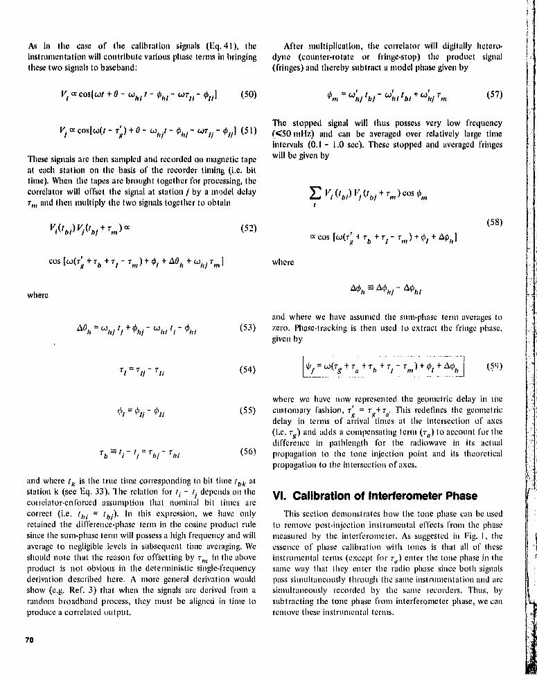
As in the case of the calibration signals (Eq.41), theinstrumentation will contribute various phase terms in bringing
these two signals to baseband:
After multiplication, the correlator will digitally hetero•dyne (counter-rotate or fringe-stop) the product signal
(fringes) and thereby subtract a model phase given by
11 a cos(wt +0 - wet t - 0111 - WTIt - oil ] (50)
V/ a cos(w(t - 7,g) + 0 - w►t/t - - wTt/ - O1/ ] (5I )
These signals are then sampled and recorded oil tapeat each station oil basis of the recorder tinting (i.e. bittime). When the tapes are brought together for processing, the
correlator will offset the signal at station j by a model delay
Trt, and then multiply the two signals together to obtain
O►n- W l,/tb/-Wl, ltbl+w ►qTm (57)
The stopped signal will thus possess very low frequency(<50 midi) and call averaged over relatively large timeintervals (0.1 - LO sec). These stopped and averaged fringeswill be given by
E1/1 (till ) V/ (tbj + Trrt) CUs Om
t
VMbl) V/(tb/ + T»,) a (52)CC COs (CJ(T i Tb + Tl - Trrt ) + chl + ^^'Ir ]
(5g)
COS (W(T9 + Tb + Tt - Ttr, ) + Of + DO ►, + W►t/ Tin ]
where
where
AN — AN/ - AN t
A011 wit/ t/ + Ob/ - will t i - oil
1 (53)
Tt = T►/ - T1! (54)
01 = 01/ - Oil (55)
Tb = t1 - t1 = Tbj - Tb1 (SG)
and where tk is the true time corresponding to bit time t bh atstation k (see Eq. 33). 1t ►e relation for t 1 - t1 depends on thecot reiator-en forced assumption that nominal bit times arecorrect (i.e. t 11 = i ll/). In this expression, we have onlyretained the difference-phase term in the cosine product rule
since the sum-phase term will possess a high frequency ; ► nd will
average to negligible levels in subsequent time averaging. We
should note that the reason for offsetting by Trr, in the above
product is not obvious in the deterministic single-frequency
derivation described here. A more general derivation wouldshow (e.g. Ref. 3) that when the signals are derived from a
random broadband process, they must be aligned in time to
produce a correlated output.
and where we have assumed the sum-phase term averages tozero. I'thase-tracking is then used to extract the fringe phase,
given by
=W(T^' + T
tt +'rh t+T T its
)+0I +A h 09,
where we have now represented the geometric delay in thecustomary fashion, T' = r + T . This redefines the geometricdelay in terms of arrival times at the intersection of axes(i.e. Tv ) and adds a compensating term (T„) to account for thedifference in pathlength for the radiowavc in its actual
propagation to the tone injection point and its theoreticalpropagation to the intersection of axes.
VI. Calibration of Interferometer PhaseThis section demonstrates how the tone phase
call used
to remove post-injection instrumental effects from the phase
measured by the interferometer. As suggested in Fig. I, the
essence of phase calibration with tones is that all of theseinstrumental terms (except for T„) enter the tone phase in the
same way that they enter the radio phase since both signalspass simultaneously through the same instrumentation and aresimultaneously recorded by the same recorders. Thus, bysubtracting the tone phase from interferometer phase, we can
remove these instrumental terms.
70

Phase calibration will be applied as follows, For eachstation, tone phase is extracted from the stopped tones givenby Eq. 15 (for example, by computing the inverse tangent ofthe ratio of real and imaginary parts). If we difference tiremeasured tone phase between stations, we obtain
01(w) = Oo1(w) - A¢j(w) (60)
TBiVS -TBWS - Ta +Tu +Tin (06)
Station calibration will provide measurements of the cabledelay T„ and intersection-of-axis delay T. so that they callremoved. The model delay TM is very accurately known, ofcourse, and can be removed exactly. Thus, we finally obtainthe desired quantity — a measured delay containing onlygeometric delay and clock offset:
which, according to Eq. 46, is given theoretically bywhich is given theoretically by
Ot(w) = CJ(Tb + v J - Ird + 01 + A01, (61)
where
Tt = T t' - Ttl
We have assurned here that the calibration phase at a givenfrequency w call obtained by interpolation (or some otherprocess) from the measured phases of the tones. Further, weneglect small doppler-shift effects, which produce frequencyshifts of the order of a hundredth of a 'bandwidth but can beaccounted for. When this calibration phase is subtracted fromthe fringe phase (Eq. 59), we obtain
^ (w) _ Of' - or (62)
which is given theoretically by
0(w)=w(T9 +TC +ra- Tit - T ,n ) (63)
where we have used Eq. 42 to show explicitly the clock.synchronization offset TC and the cable delay TU , We have nowobtained a measurement of interferometer phase that is free ofthe instrumental terms calibrated by tone phase,
Once the interferometer phase has been corrected with tonephase, one can readily obtain the delay by the bandwidthsynth,sis (BWS) technique of taking the difference betweenthe phases at frequencies wa and cob:
T' kcia) - O(wb)
(64)B IVS W - Wa b
which is given theoretically by
TB{VS Tg + T + 7 - Tu - T in (65)
T BWS _ T + Ti, (67)
The clock offset T. is the only remaining instrumental tern.This term represents the synchronization offset betweenstation clocks (T,j T^!) and pertains to the clock referencepoints, established by the definition and removal of the cabledelays, T«.
(We should note here that the aforementioned DSNcalibrator system will have the capability of compensatingon-site for the cable delay up to the tone generator b:rapplying a calibrated advance to the phase leaving the cable,stabilizer. In this case, T„ in earlier equations would be equalto the small delay through the tone generator up to theinjection point.)
As indicated previously, certain conditions must be met forthis calibration analysis to be valid. First, the model for theheterodyne phase must be identical in the model phases usedfor fringe-stopping and tone-stopping. The calibrator signalmust possess a low fractional power level. Tone frequenciesmust be chosen to handle phase variations across each channelpassband, if such variations are present at a significant level.
In the calibration process described above, a subtle pointhas been neglected. Only the fractional part (in cycles) of boththe interferometer phase and tone phase can be detenmined
when please is extracted after counter-rotation. The integer.cycle part of phase can not be determined by this processalone. Thus, when tone phase is subtracted from inter-tbromete; phase, the subtraction actually denotes removal ofthe fractional part of instrumental phase. We can ignore allinteger cycle errors at this point since we realize that there areinteger cycle ambiguities due to delay modeling that must beresolved later in the BWS process. The BWS process onlyrequires as input precise values for the fractional part of phase,free of unwanted instrumental phase (fractional part). Tileinteger-cycle part (due to Tg and T,) is then added in arecursive process to be described in a later report. The outputis a delay Measurement free of post-injection instrumental
71
effects. It is a peculiarity of this technique that, even thoughdelay and interferometer phase can be ultimately calibratedabsolutely with regard to instrumental effects, instrumentalphase, including integer cycles, is never absolutely measured.
VII. Remaining WorkSome important issues related to system calibration remain
to be considered. for lack of adequate information concerning
system characteristics (e.g., phase ripple and variability), thireport has made no effort to assess the accuracy with whiclsystem calibrations can be carried out. This is obviouslycrucial question that should be addressed as soon as possibleSuch . , t accuracy analysis would have to consider the approximations, if any, that are imposed by practical consideration!during implementation and will be intimately connected withthe determination of the optimum number of tones and powerlevel.
r'
References
1. A. E. E. Rogers, "A Receiver Phase and Group Delay Calibrator f'or Use in Very LongBaseline Interferometry," Haystack Observatory Technical Note 1975.6.
2. J. L. Fanselow, "The Use of a Phase Calibrator in VLBI to Remove Receiving SystemPhase Shifts," JPL IOM 315.2.01 1 (in internal document), Oct. 1976.
3. J. B. Thomas, "An Analysis of Long Baseline Radio Interferometry," JPL USNProgress Report 32-1526, Vol. V (1971).
ORIG11,4AL PAGE 1bOF POOR QUAWT
72

x
CALIBRATIONSIGNAL(DELAY T)
HETERODYNE SIGNAL*h = "ht + Oh
.. ^.
^C = we (t + TC - Tu )
T^GENERATOR
ltit = 4/t+o
PHA% OF SIGNAL
-(t + T` - TV)(IN OR
wt +e
AMPLIFIER, 1(
DELAY Tl _/
`
FILTER #-SHIFT ¢
(TONE AT w)
(RADIO SIGNAL AT ^)
(1) 41 = 41In - 1 - 0,
(2) 02=0In- "I-01 -*h
SAMPLER ANDRECOR--
(OUT) 4Wt(tbi) = Oin (ti) - -li - 0. - *h
WHERE tbi = ti + c - Tr
TIMING SIGNAL(DELAY r, RELATIVE TO P)
P_CABLESTABILIYXR
CLOCK REFERENCEPOINT
OC = WC (t + C)
FREQUENCY STANDARD
Fig. 1. Simplified illustration of VL81 instrumentation
VW
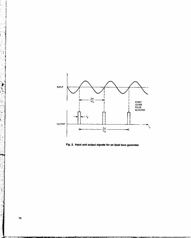
INPUT
-C I EVERY
OTHERPULSE
BLANKED
— ► rP
1 1
OUTPUT —^f
fw
—^oP•
^' P
Fig. 2. Input and output signals for an Ideal tone generator
74

DSN Progress Report 42 . 44
January and February 1978
N78-24221
An Analysis of Viking S-X Doppler Measurementsof Solar Wind Columnar Content Fluctuations
P. S. CallahanTracking Systems and Applications Section
More than 320 passes of Viking S Doppler data have been used to investigatecolumnar content fluctuations in the solar wind from 19 August, 1976 to 28 February,1977 These data are used to estimate the power spectrum and radial dependenceof solar wind density fluctuations. It is found that: (1) the electron density fluctuationsdecline with heliocentric distance as r-1-8 r 0.1; (2) the power spectrum depends oilfluctuation frequency as v-2.5 t 0.2, These results are used to predict range change as afunction of time scale and sun-earth-probe angle. Changes of interest for advancednavigation techniques are found to be likely.
I. IntroductionThere is continuing interest in the errors introduced into
radio metric tracking by the solar wind (SW) plasma. In orderto estimate these errors a large amount of Viking SA Dopplerdata measuring the change in electron columnar content hasbeen analyzed. Because the density fluctuations (DF) are of arandom nature the analysis has been done in terms of thepower spectrum and the changes in spectral amplitude withheliocentric distance extracted.
A long term goal for the DSN is a predictive model of radiometric data quality. This analysis is a major first step inbuilding that model as it provides the large-scale radial andtime variations of the SW plasma. It remains to compare theresiduals from these large-scale models to solar surface andother SW data to develop the detailed predictive model.
A preliminary report of the present analysis (but with onlyhalf the amount of data) was given in Ref. I. The major
differences between the findings there are (1) a revision of thespectral index from -3.0 to -2.5; and (2) a deletion of thediscussion of sunspot cycle effects. It has become clear that alonger time base of measurements will be needed to discusssunspot cycle effects.
The data coverage for this analysis is described in Sec-tion II. The analysis procedures are outlined in Section III.Section IV gives the results and discusses the implications forradio metric data.
II. Data CoverageThe data coverage for this analysis is shown in,Table 1. The
data are given in the groups in which they were averaged todetermine the radial dependence of the power spectrum. Thedates are in the format YYMMDDHH (year, month, day, hourat beginning of pass). Superior conjunction was taken to be1976 November 25,'00 hours.
75
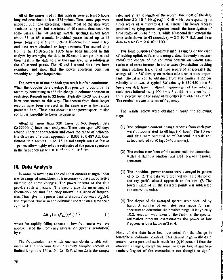
All of the passes used in this analysis were at least 5 hourslong and contained at least 275 points. Thus, some gaps wereallowed, but none exceeding 1 hour. Most of the data were1-minute samples, but stretches of 10-second data occur insome passes. The net average sample spacings ranged fromabout 55 to 65 seconds. Individual passes lasted up to 12hours. Near and after conjunction 10-second and some 1 sec-ond data were obtained in large amounts. Ten second datafrom 8 to 15 December 1976 have been included in thisanalysis by averaging the data to 30-second sample times andthen treating the data to give the same spectral resolution asthe 60 second passes. The 10 and I second data have beenexamined and show that the power spectrum continuessmoothly to higher frequencies.
The coverage of one or both spacecraft is often continuous.When the doppler data overlap, it is possible to continue therecord by continuing to add the change in columnar content ateach step. Records up to 32 hours (typically 15 .20 hours) havebeen constructed in this way. The spectra from these longerrecords have been averaged in the same way as the resultspresented here. These data show that the power spectrum alsocontinues smoothly to lower frequencies.
Altogether more than 320 passes of S-X Doppler data(';b 3000 hrs) have been analyzed. These data span ±95 daysaround superior conjunction and cover the range of heliocen-tric distances of closest approach of 0.031 to 0.487 AU. Con-tinuous data records up to 32 hr and sample rates as fast as1 per sec allow highly reliable estimates of the power spectrumin the frequency range 1 X 10- 4 to 2 X 10- 1 I-Iz.
III. Data AnalysisIn order to investigate the columnar content changes under
a wide range of conditions, it is necessary to have an objectivemeasure of these changes. The power spectra of the dataprovide such a measure. The spectra give the mean squaredfluctuation per unit frequency interval in a range of frequen-cies. Thus, given the power density at some frequency, Po f(v),the expected change in the columnar content on a time scaletl = I /v is
AI(tt)= (Pot(v)*V) 112 (1)
where for rapidly falling spectra at low frequencies we haveapproximated the frequency interval Av (spect al resolution)by v.
The frequencies over which one can obtain reliable esti-mates of the spectrum from discretely sampled records oflimited length are 1/4 At > v > 10/T, where At is the sample
rate, and T is the length of the record. For most of the dataused here 3 X 10 -4 Hz <, v., 4 X 10- 3 Hz, corresponding totimes scales of 4 minutes q6 tr <, 1 hour. The longer recordsproduced by tying passes together permit the investigation oftime scales of up to 3 (tours, while 10-second data extend thetime scale down to 40 seconds (v 2 X 10' 2 Hz), and 1-secdata to 4 sec (v 2 X 10' 1 Hz).
For some purposes (near-simultaneous ranging or the errorof making uplink calibrations using a downlink-only measure-ment) the change of the columnar content on various timascales is of most interest. In other cases (two-station trackingor single station tracking of two separated spacecraft) thechange of the SW density on various cale sizes is more impor-tant. The latter can be obtained from tite former if ttte SWvelocity is known. A typical SW velocity is 350.450 kill s- ► .Since our data have no direct measurement of the velocity,scale sizes inferred using 400 km s- r could be in error by upto 50 percent sir ;e the range of velocities is ^300 .700 km s- ► .The results here are in terns of frequency.
The results below were obtained through the followingsteps:
(1) The columnar content change records from each passwere autocorrelated to 60 lags (^-1 hour). The 10 sec-ond data were summed to ^-30-second intervals andautocorrelated to 80 lags (^-40 minutes).
(2) The cosine transform of the autocorrelation, smoothedwith the Harming window, was used to give the powerspectrum.
(3) The individual power spectra were averaged in groupsof 5 to 12. The data were grouped by the distance ofthe ray path's closest approach to the sun, Q. Thelowest value of all the averaged points was subtractedto remove the noise.
(4) The slopes of the averaged spectra were obtained byhand. A number of estimates were made for eachspectrum to determine the possible range. It is typically±0.2. Account was taken of the fact that the spectralestimation program overestimates the power at lowfrequencies by a factor of 2 to 4.
None of the data have been corrected for the change inionospheric columnar content. This change is generally .x,1.5meters over a pass and so is much less (<,10 percent) than theobserved changes, except for some passes in August and Sep-tember. Neglect of this correction is not thought to signifi-
76

cantly affect any of the final results. Care was taken, especiallyfor data taken very near the sun, to insure that slipped cycleswere not added to the columnar content change. Apparentcolumnar content changes greater than 2nt/min were never
allowed and in most cases tighter limits were imposed.
fit to the power spectrum analysis, the individualand long records were examined for rats variation about themean, peak-to-peak change, maximum rate of change, andcharacter (slope, single or multiple "humps," and time scale ofsignificant change) of the change, The numerical indices are allclosely related to the power spectrum. The character of thechange allows some investigation of changes oil longer timescales than call done formally with the power spectrum.
IV. Results and DiscussionFrom the general character of the columnar content
changes, especially those seen on the long (tied) passes, onecan see that the power spectra extend to low enough frequen-cies to pick up most of the important changes. Occasionally,there are slopes or "humps" with time scales of 8-12 hours,but these occur only about once per month. At the fastestsample rates, the character of the columnar content is verysimilar, though of reduced amplitude. Thus, the data from thepower spectra provide a fairly complete and realistic descrip-tion of the columnar content changes for time scales from 2seconds to several hours.
The spectral index range for each averaged spectrum isgiven in the last column of Table 1. The indices were estimatedby hand on plots of the averaged spectra. The average andstandard deviation of the upper and lower estimates are respec-tively Q„ = 2.63 ± 0.18, PL = 2.40 t 0.16. The value Q = 2.5 t0.2 will be adopted for the spectral index of columnar contentfluctuations. It is in good agreement with Ref . 2 and 3 andother recent work on SWDF. Examination of averaged spectraof data records in which passes were tied together to give totalrecord lengths of 20.30 fir show that this spectral index ismaintained down to v ^?5 1 X 10- 4 Hz. As discussed above thespectral estimation program overestimates the power at lowfrequencies. This effect is important, (approximately a factorof 2) at 3 X 10- 4 Hz for single pass records. Thus, for reliableresults the scaling law v' 2.5 should only be applied to P(F2 =6 X 10⁻⁴ Hz) data in Table 1.
Data sampled at once per second and once pei 10 sec wereused to investigate the high frequency portion of the spec-trum. It was found that at the highest frequencies, 1 X 10- 2 '<'v < 2 X 10- t , the spectrum flattened somewhat to 2.1.E 04,2.3. Below v a5 1 X 10- 2 Hz the spectral index remained at Q
2.5. Three sets of I sec. data (of 6 obtained) showed
discrete spectral features at frequencies of about 1.5 X 10- ►Hr,. The periodic (period En 7 sec) disturbances lasted for aboutI (tour fit case. The spectral amplitude Indicates columnarcontent changes of about 9 X 10 9 ctn-2 w 8 X 10" 4 m(1) ofone-way S-band range change. The explanation of the featureshas not been found.
In Fig. I, the averaged power density 3 X 10-° 4 IIz is plotted
against Q, the distance of the ray path's closest approach tothe sun. The line through the points has slope 2.6. Note thatthe Mariner points generally lie above the Viking points, Thepoints at large Q may be biased upward by the ionosphere.These data overestimate the true spectral amplitude by afactor of 2.
To investigate the radial dependence more quantitatively, acomputer program was used to find the RMS deviation about aseriez of models characterized by a radial exponent, y and anellipticity e. The ellipticity was included because the solarcorona is known to be reduced near the poles at sunspot cycleminimum. The model used was
P cal d ° Pors (41/0.1 AU)t3+2ti) (1 + e Sin (fat))2
(2)
where Q is the distance of closest approach (column 5 of Table1) and Lat is the heliographic latitude of tine point of closestapproach (column 6 of Table 1). The parameters which pro-duce the smallest RMS of the scaled spectral estimates abouttheir average were y = -0.2 t 0 . 1 and e = 0 . 6 t 0.6. The datashow no strong preference for any value of e, but do clearlyshow that y is less than 0.
A decline of the spectral amplitudes of Q-2.6 implies (foran approximately constant radial SW velocity) that SWDFdecline as Sir « r- 1 - 8±0 - 1 . This result is also found in ananalysis of Doppler Noise data (Ref 3 and 4). It implies thatthe relative density cltaages become larger with radius, (since ndeclines at least as fast as r' 2 ), although this conclusion maybe modified somewhat by including the acceleration of the SWnear (r — 3 to 30 Ro = 0.015 to 0.15 AU) the sun.
The data in Table I are well-summarized by the function
P(v,Q) = (4.0 t 2.0) X 1030 Q
)- 2.6±0.1
O. I AU
(_ V ) -2.5±0.2
4c1-414 Z 1
3 X 10'(3)
n
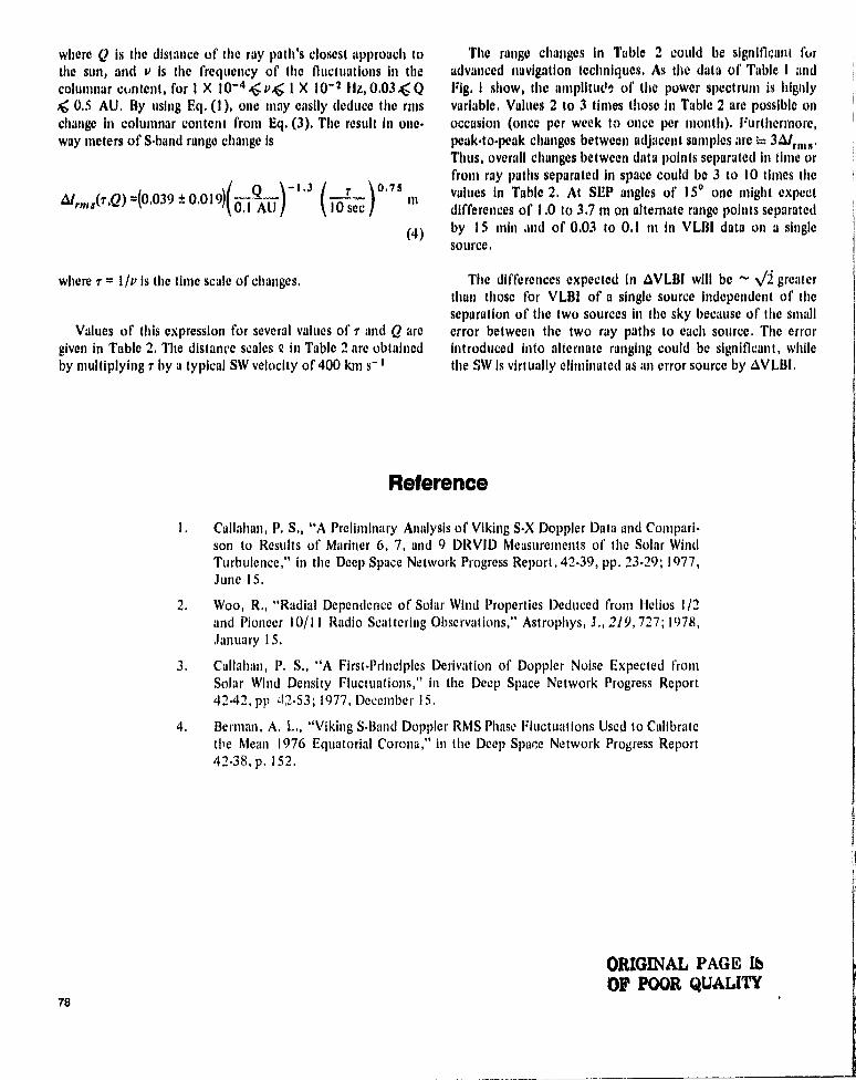
where Q is the distance of the ray path's closest approach tothe sun, and v is the frequency of the fluctuations IIIcolumnar content, for I X 10-44V4 I X 10 ° 2 IIz, 0.03 4 Q< 0.5 AU. By using Eq. (I), one may easily deduce the rmschange III content from Eq. (3), The result in one•way meters of S-band range change is
Alrms(r+Q)'"0.039 t 0.019)(0,1—Q I.J
AUr e.75
In10 sec
(4)
where r = 1 /v is the time scale of changes.
Values of this expression for several values of r and Q aregiven in Table 2. The distance scales ¢ III 2 are obtainedby multiplying r by a typical SW velocity of 400 km s-1
The range changes III 2 could be significant foradvanced navigation techniques. As the data of Table I andFig. I show, the amplitucte of the power spectrum is ltignlyvariable. Values 2 to 3 times those hi Table 2 are possible onoccasion (once per week to once per month). furthermore,peak-to-peak changes between adjacent samples are '= 3A/r1111VThus, overall changes between data points separated in time orfrom ray paths separated in space could be 3 to 10 times thevalues III 2. At SEP angles of 15 0 one might expectdifferences of 1.0 to 3.7 in alternate range points separatedby 15 min and of 0.03 to 0.1 in VLSI data on a singlesource.
The differences expected In AVLBI will be N N/2 greaterthan those for VLBI of a single source independent of theseparation of the two sources in the sky because of the smallerror between the two ray paths to each source, The errorintroduced into alternate ranging could be significant, whilethe SW is virtually eliminated as nn error source by OVLBL
Reference
I . Callahan, P. S., "A Preliminary Analysis of Viking S•X Doppler Data and Compari.son to Results of Mariner 6, 7, and 9 DRVID Measurements of the Solar WindTurbulence," in the Deep Space Network Progress Report, 42.39, pp. 23 .29; 1977,June 15.
2. Woo, R„ "Radial Dependence of Solar Wind Properties Deduced from Ifelios 1/2and Pioneer 10/11 Radio Scattering Observations," Astrophys, J., 219,727; 1978,January 15.
3. Callahan, P. S., "A First-Principles Derivation of Doppler Noise Expected fromSolar Wind Density fluctuations," in the Deep Space Network Progress Report4242, pp, .12-53; 1977, December 15,
4. Berman, A, L., "Viking S•Band Doppler RMS Phase fluctuations Used to Calibratethe Mean 1976 Equatorial Corona," i ►t the Deep Spare Network Progress Report42.35, p. 152.
ORIGINAL PAGE IbOF POOR QUALITY
78

Tayie 1. Averaged sp "s of Ming S-X doppiel dOb'
$O. Q Avg Avg ObsObs Days from Sup. Conjunction P(Fl), Scaled for p(F2), Scaled forFirst Date Last Date Avg SC (O.iAC) Lat P (F1) a
P (F2) b First Last Avg Radial Radial + Lat Radial Radial + Lat
760132116. 760820to. t0. 30. 4.670 3.o .137.30 .124.29 -9S.33 -90.33 -94.03 .4046939 .3660.30 .3707.29 .3320929 2.55-2 .6576082708. 76090100. 11. 30. 4.590 3.4 .768929 .718928 -89.67 -85.00 -87.33 .2044930 .1846930 .1062929 .1662929 2.7 -2.97 60 9 0117. 76090016. tu. 30. 4.300 3.8 .164930 .180.29 -04.29 -79.33 -01.61 .3637930 .3315 930 .3992929.3630929 2.5-2.;7bn90708. 76091016. 6. 30. 4.070 4.1 .142930 .i1S929 -78.67 -75.33 -77.00 :.2760930 .2433 930 .2235929 .2052929 2-5-2-77b090916. 76091522. 12. 27. 3.830 4.4 .690929 .649928 -76.33 -70.00 -73,21 .1159930 .1071930 .1090929 •1000929 2-3-2-676091700. 76092121. 11. 27. 3.500 4.8 .446930 .452929 -69.00 -64.12 -66.56 .6035930 .5627936 .6116929 .5703929 2.3-2.5576101806. 76102721. 8. 30. 1.090 6.2 .229931 .323930 -37.67 -28.13 -32.90 .SZ09*30 .5194930 .7615929 .7326929 2.5-2.75701020;1. 76103111. e. 27. 1.090 6.2 .136931 .103938 -3S.S4 -24.54 -30.04 .2370930 .2276930 .1705924 .1726 929 2.3-2.776110100. 76111320. 9. 30. .460 S.4 .536931 .506930 -25.00 -11.17 -17.58 .3452.30 .3071930 .3070929 .2099929 2.4-2.6+6110121. 76110721. 7. 77, 1.070 S.9 .609931 .638930 -23.12 -17.12 -20.12 .4791930 .4578930 .S922929 .4796929 2.35-2.67+76112619. 76120,20. 1. do. .266 -a2.9 .113933 .127.32 1.79 7.63 4.61 .3749930 .5244930 .4214929 .5094929 2.25-2.3576;20800. 7612;522, 6. 20. .908 -12.1 .187932 .67 7930 13.06 20.92 16.06 .9947930 .1092931 .3594929 .3953929 2.6-22-87 bl2311 9. 77010503. 0. 30. 1.910 -10.2 .153931 .214930 36.79 41.12 38.96 .4639930 .5092930 .6768929 .7122929 2.6-2.8"77010416. 77010901. S. 30. 2.040 -10.0 .226931 .20S930 40.67 45.04 42.05 .6371930 .6769930 .7493929 .7954929 2.6-3-07 7910518. 77010803. S. 27. 2.000 -10.0 .570930 .600929 41.75 44.12 42.94 .2161930 .2264930 .3033929 .3170929 2-3-2-47 7 011100. 77011205. S. 27. 2.260 -9.7 .451930 .SAS*" 41.00 48.21 47.60 .2211930 .4300930 .2491929 .2S9a929 2.4 -2.777011216. 77011516. S. 30. 2.3bo - 9.6 .121930 .11a929 46.75 51.75' Seas .6356929 .6600929 .SG4S*a8 .6109920 2.35-2.7.7011823. 77012014. 5. 30. 2.o20 -9.2 .357930 .311929S4.06 S6.S9 SS.77 .2411 930 .2479930 .2100.29 .a1609a9 2.3 -2.a^77013122. 77020818. 8. ?7. 3.330 -8.0 .134931 .204929 67.92 7S.7S 11.83 .1609931 .1610931 .3306929 •3300929 2.355-2.677021518. 7702231S. 6. 27. 3.870 -6.6 .630930 .510949 02. 7S 90.63 86.69 .100S931 .1050931 .0021929 •0696929 2.1 -2.37702?200. 77022618. 7. V. 4.070 -6.3 .135930 .4778.29 69.00 95.75 92.37 .2624930 .2530930 .5403929 .5269 929 2 .1 2.44
a) Fl-3z10-%tb) F2-6=104Hz
The scaled spectral estimates have been scaled by (Q/0.1 AU )2.6 and/or 0 + 0.6 sin(Lat) )2 and them divided by the avereps of then factors(19.46 and 1.19) for the whole data set.
vto

Table 2. Alan, (r, 0) in one-way 5•band motors.f • r x 400 km /soc
?Wc) = 3000 1000 100 30 10 3Min) = 1.2+F, 4+5 4+4 1.2+4 4 +3 1.2+1
Q(AU) SL P Glrnt^ (nt)
.05 2.9 6.86 3.01 .535 .217 .0952 .0386
.10 5.7 2.79 1.22 .217 .0881 .0386 .0157115 8.6 1,64 .721 .128 ,0520 .0228 0092.20 11.3 1.13 ,496 .0883 .0358 .0157 ,0064
.25 14.5 .846 .371 ,0660 .0268 .0117 .0048
.30 17,5 .668 .293 .0521 .0211 .0093 .0038
.40 23.6 .459 .201 .0358 .0145 .0064 .0026
.50 30,0 .344 .151 .0268 .0109 .0048 .0019
Y AGE 10
80
& Y

Q, AU
Fig. 1. Averaged spectral amplitudes
®T®
^®Cgl
®AND 7 (1969)
DRVID DATA® /®® MARINER 9 (1971)
DRVID DATA
® VIKING AS-X DOPPLER DATA
® ® VIKING BS-X DOPPLER DATA
®® ® Q+ VIKING A AND BS-X DOPPLER DATA
®® () VIKING A AND B10-s S-X DOPPLER DATA
100 10-1
10-2 10-3
1033
1032
1031
^Nx
YEU
uY0
xM
dd 1030
1028
1029
V 81

DSN Progress Report 42.44
January and February 1978
N78-24222
A Method for Measuring Group Time Delay Througha Feed Horn
T. Y. Otoshi, R. B. Lyon, and M. FrancoRadio Frequency and Microwave Subsystems Section
A technique is described for measurement of time delay through a feed horn. Tiletechnique consists of measuring the time delay between the input and output ports oftwo identical horns separated by a known airpath distance. Ground multipath signals,which normally produce errors in this type of measurement, were identified andeliminated by using a time domain technique. Experimental results at 2113 MHz showedgood agreement with calculated values.
I. IntroductionGround station delays for 64•m antenna Deep Space Sta-
tions (DSS) are currently being calibrated by the TranslatorMethod. As described in References 1 and 2, the major portionof the ground station delay is measured e'uring pre- and post-track calibrations by this method. The remaining (smaller)portion of station delay is calculated and assumed to be timeand frequency invariant. One of the more difficult com-ponents for which delays are calculated is a complex feed hornassembly. The current feed horn assembly used in the S-BandPolarization Diversity (SPD) Cone used on 64-m antennasconsists of orthomode transducers, quarter wave plates, modegenerator, and a corrugated horn. Calculated delay values forthese components have been reported in Reference 3. Themonopulse feed horn assembly used in DSN 26-m antennasystems is even more complex and no simple method is cur-rently known to the authors for calculating delays of mono-pulse feeds. The current use of dish-mounted zero delay de-vices (Ref. 1) for ranging has made it unnecessary to determine
the delay of the monopulse feed. However, it may becomeimportant to determine 26-m antenna monopulse feed horndelays in the near future for such projects as the VLBI TimeSync Experiment and VLBI Validation Project.
This article presents a method which can be used to experi-mentally determine the delay through a feed horn assembly.The technique was used on simple standard gain horns, but canbe extended to complex feeds.
IL Test SetupThe method to be described is very similar to the antenna
gain measurement method discussed by Silver (Ref. 4) andBeatty (Ref. 5). The method consists of using an antennarange where two horns (or antennas) are separated by a knownphysical distance R as shown in Fig. 1. Figure 2 shows theactual test setup on the antenna range located on the SouthEnd of the JPL Mesa Facility. The standard gain horns are
62

mounted on two antenna towers, one of which is rotatable andcan be moved axially on a rail in the direction of the mainbeam. The second tower Is stationary but permits a mountedhom to be adjusted in a vertical direction. Both horns weremounted at a height of 5.55-m above the ground and 1-mabove the top of tine roof of Mesa Building 212. The hornsbeing tested are Scientific Atlanta Model (12 . 1.7) pyramidalhorns. The horns were separated at distances varying from152.4 cm (5 ft) to 1676.4 cm (55 A) in 152.4 cm (5 ft)Increments. The smallest and largest separation distances cor-respond to 1.6D 2 /A and 17.5D 2 /A, respectively, where D Is thewidest opening of the horn equal to 36.88 cm (14.52 inch)and A is the free space wavelength of the test frequency of2113 MHz.
The basic instrument used to measure delay was a ScientificAtlanta Fault Locator Model 1691 shown in Fig. 3. Thisinstrument was developed to be portable for field use and isnormally used as a high resolution time domain reflectometerto locate discontinuities (faults) in microwave antenna trans-mission lines. For the results of this article, this instrumentwas temporarily modified to measure transmission time delay.The absolute accuracy of the modified instrument is estimatedto be better than ±2 ns and the resolution is about t0.2 ns. Themain advantage of this instrument is in its time domain logicwhereby the time delay of the primary (desired) signal can beisolated and measured separately from the effects of otherundesired signals such as from ground multipath.
Figure 4 shows typical X-Y recording of this instrument forhorn separation distances of 152.4 cm (5 ft) and x04.8 em (10ft).* The recordings show only primary signals because multi-path signals were at least 35 dB down from the main signalamplitude in the particular test setup used. The basic measure-ment technique is described as follows. As indicated by theblock diagram of the test set-up shown In Fig. 1, measure-ment of the time delay is made of the total system whichincludes the delays of the two horns, airpath, cables, amplifierand the Fault Locator instrument. Then a reference measure-ment is taken by disconnecting the cables at the input andoutput of the coax-to-waveguide transitions and then connect-ing the cables together with a coaxial adapter or pad insertedbetween them. Subtraction of this reference measurementfrom the test measurement values results in the delays of onlythe two horns plus waveguide transitions plus airpath. Afterfurther subtraction of (1) the airpath delays, (2) the delays ofthe waveguide-to-coax transitions, and (3) making a small cor-rection for coaxial adapters used, then one arrives at the delaysof the two horns only if the two horns are identical, the delayof a single horn is obtained by dividing the result by 2.
*The use of the Fault Locator in a transmission mode rather than thereflectometer mode required that the indicated instrument readings bemultiplied by 2 as shown in the table iu Fig. 4.
Tile airpath delays are easily calculable from precise meas-urements of the physical separation distance R between thehorn apertures using a plumb bob and a steel tape measure.The delays of the two waveguide transitions are determined bymeasuring them separately at the same test frequency by useof a network analyzer.
III. Test ResultsTable 1 shows test results of measurements made at 2113
MHz. It can be seen that the horn delay measured at thelargest separation I7.SD 2 /X does not differ from the measuredv ae at the smallest separation 1.6D 2 /X by more than 0.41 ns.At very close distc,,ices, multiple reflections between hornscannot be isolated by the Fault Locator. Figure 5 shows thetheoretical calculated delay for a single horn at 2113 MHz.This calculated delay of 1.39 ns is based on the theoreticalgroup velocities in the constant and tapered section of thehorn at 2113 MHz. It can be seen that the calculated andmeasured delays in Table 1 are in agreement to within ±03 ns.
The entire set of measurements was again repeated withabsorbers placed on the ground midway between the horns ateach separation distance. A slight (but non-significant) im-provement in agreement was obtained between theoretical andmeasured values. It was concluded that absorbers would notgenerally be needed for most test setups.
Although the Fault Locator instrument is not Intended to beused for accurate gain measurements, relative amplitude dataaccurate to ±0.5 dB is simultaneously available and can beused to provide a good cross check on the experimental setup.Amplitude data obtained from recordings such as the oneshown in Fig. 4, were used to calculate horn gain. For thevarious separation distances shown in Table 1, the measuredhorn gains agreed to within 1 dB of the theoretical value of15.95 dB at 2113 MHz.
IV. Conclusions and Future ApplicationA technique has been presented for the measurement of
time delays of a feed horn. The technique presented in thisarticle involves the measurement of the time delay of apyramidal standard gain horn. This technique can be extendedto make measurements of corrugated standard gain horns,spacecraft antennas, and most non-dispersive types of complexfeed assemblies used in the DSN. Two identical feeds are notrequired if the delay of a simpler horn of the same polarizationhas already been determined.
The measurement technique is not necessarily restricted tothe use of a Fault Locator (such as described in this article)provided that it is already known that the antenna range is free
83

from multipath errors. In such a case, a network analyzer canbe used and possibly give more accurate time delay measure-nrents over frequency intervals (spanned bandwidths) of about20 to 40 MHz. However it most cases, the sources of groundmultipath and multiple reflection are generally not known and
special time consuming techniques must be employed tominimize or identify their effects. The Fault Locator timedomain Instrument provides a simple method for quicklyidentifying and making a direct measurement of the time delayof only the desired primary signal to accuracies of about ti ns.
Acknowledgement
The modification of the Fault Locator was suggested and accomplished by A. RayHowland, JPL consultant and President of the Howland Company at Atlanta, Georgia.
References
1. Kumarek, T., and Otoshi, T., "Terminology of Ranging Measurements and DSSCalibrations," in the Deep Space Network Progress Report 42.36, pp. 3540, JetPropulsion Laboratory, Pasadena, Ca., Dec. 15, 1976.
2. Otoshi, T. Y. et al, "Calibration of Block 4 Translator Path Delays at DSS 14 and CTA21," DSN Progress Report 42-37, pp. 188. 197, Feb. 15, 1977.
3. Otoshi, T. Y., Wallace, K. B., and Lyon, R. B., "Dual Coupler Configuration at DSS 14for the Voyager Era," DSN Progress Report 42.42, pp. 184-195, Dec. 15, 1977.
4. Silver, S., "Microwave Antenna Theory and Design," Radiation Laboratory Series,Vol. 12 McGraw Hill, 1949, pp, 582-585.
5. Beatty, R. W., "Discussion of Errors in Gain Measurements of Standard Electro-magnetic Horns," NBS Technical Note 351, National Bureau of Standards, March1967.
84

Table 1. Scientific-Atlanta Model 12 .1.7 Standard Gain HornDelay measurement results at 2.113 t9Ma
Horn separation O ® © ® 0n - nWaveguide
Airpath Net transition Two SingleRX delay measured pair horn horn
R, R, D' rR, dclay,a delay, delay,b delay,ft cm ns ns ns ns ns
55 1676.4 17.5 55.92 60,39 1.44 3,03 1.5250 1524.0 15,9 %84 55.11 1.44 2.83 1.4245 1371.6 14.3 45.75 50.02 1.44 2.83 1.4240 1219.2 12.8 40.67 44.73 1.44 2.62 1.3135 1066.8 11.2 35.58 39.45 1,44 2.43 1.2230 914.4 9.6 30.50 34.97 1.44 3.03 1.5225 762.0 8.0 25.42 29.48 1.44 2.62 1.3120 609.6 6.4 20.33 24.40 1.44 2.63 1.3215 457.2 4.8 15.25 19.11 1.44 2.42 1.2110 304,8 3.2 10.17 14.03 1.44 2.42 1.21
5 152.4 1.6 5,08 8.74 1,44 2.22 1.11
a Nct delay results from subtracting Fault Locator reference readingfrom test reading in units of feet and converting the result into trans-mission delay in units of nanoseconds,
bDclay of two horns = column © data - (column (D + columndata).
as
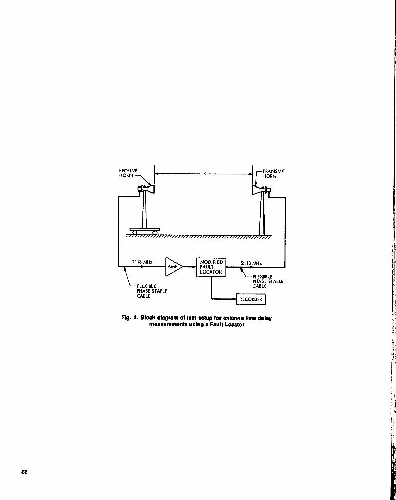
RECEIVE R TRANSMITHORN THORN
2113 MHz MODIFIED 2113 MHzAMP FAULT
LOCATORFLEXIBLEPHASE STABLE
- FLEXIBLE CABLEPHASE STABLECABLE
RECORDER
Fig. 1. Block diagram of test setup for antenna time delaymeasurements ucing a Fault Locator
86

Fig. 2. Test Setup at JPL Antenna Range Facility. Horns are 152.4 cm (5 ft) apart
71,,.,
Fig. I Scientific Atlanta Fault Locator Model 1891 and Recorder
ORIGINAL PAGE Ibof POOR QUALM
87

X - 110.3
REFERENCE
-25
X a 114.6
NOTE: SINCE THE FAULT LOCATORREADS OUT IN UNIT OF FT,IT IS NOT MEANINGFUL TOCONVERT X AXIS VALUES TOMETERS
50
100 150INSTRUMENT READING X, ft
isLi9t
•15Q
50
30200 250
R Z 152.4 em (5 ft)
X = 117.
R = 304.8 cm (10 ft)
COMPUTATIONS
INSTRUMENT TRANSMISSION DIFFERENTIALREADING, ft DISTANCE, ft DISTANCE, ft
110.3 220.6 0.0114.6 229.2 8.6117.2 234.4 13.8
Fig. 4. Sample recording of transmission distance measumment using Fault Locator
88

L10.92 cm
T
36.88 cm
1 X. dx
l i cg of [X. (X)] 2 - X02
WAVEGUIDE , cm Q , cm t nsSECTION c i fli'
CONSTANT 21.84 10.08 0.44WR430 SECTION
TAPERED MORN 21,84 -o- 26.49 0.95SECTION
TOTAL 1.39
Fig. S. Calculated time delay of standard gain pyramidal hom(Scientific Atlanta Model 12-1.7) at 2113 MHz
89

DSN Progress Report 42.44 January and February 1978
S78-24223
An Analysis of Alternate Symbol Inversion for ImprovedSymbol Synchronization in Convolutionally
Coded SystemsL. D, Baumert and R, J, McEliece
Communications Systems Res4arch Section
H. van TilborgTechnological University, Eindhoven, The Netherlands
lrr the current N SSA Planetary Fragrant Fllghtjt;rvund Data System Standard, it isproposed that alternate symbols of the output of a convolutional encoder be inverted inorder to guarantee the symbol synchronizer a certain richness of symbol transition.
/n this paper we analyze this technique; in particular we characterize those convolu-tional codes with the property that even if alternate symbols are inverted, arbitrarily longtransition free symbol streams may occur, For codes which do not exhibit this patho-logical behavior, we give an upper bound on the largest possible transition free run.
I. IntroductionMany modern digital communication systems derive symbol
synchronization from the data itself rather than from a sepa-rate synchronization channel, A common type of symbolsynchronizer, and one that has become a NASA standard, isone that includes a clock whose phase and frequency aregoverned by timing estimates derived from the received data.The performance of this kind of symbol synchronizer dependsin part on the "richness" of symbol transitions in the receiveddata. An unusually long sequence of all 0's or all 1's, forexample, could cause the local clock to lose synchronization,and so also data, temporarily.
If the data were uncoded, one possible method of increas.ing the transition density would perhaps be to add the se-
gijence .. • 10101010 • .. to the data stream, i,e„ by inverting,dternate symbols. The new data stream would then contain along transition-free string only if the original data streamcontained a long alf, -.rnat!ng string. Presumably a long alternat-ing string is less likely than a long constant string, and so thismethod would probably have the deaired effect.
If the data is encoded prior to transmission, one could againtry to increase the transition density by inverting alternatesymbols, and indeed this symbol inversion is now part ofNASA's data system standards (Ref. 3). And whereas foruncoded data one can only assert that symbol inversion willtend to increase the transition density, for convolutionallyencoded data a much stronger statement can be made: Pro-vided the code does not suffer from a certain improbableproperty, there is an absolute upper bound one can place on
90

die length of the largest possible transition-free symbol runfront the encoder, independent of the data being encoded, Forexample, the NASA standard rate 1/2 constraint length 7 hasmaximum run 14; the rate 113, constraint length 7 has maxi•mum run 12.
In this paper we shall give a general approach to theproblem of finding the largest possible encoded output of theform ' ' ' 10101010 ' ' ' from any convolutional code, in See-lion 2 we will classify all codes which admit all run ofthis type; in Section 3 we will give ;m upper bound oillargest runs for codes which do not admit all run; InSection 4 we work some specific examples; and in the Appen•dix we collect some known results about convolutional codeswhich we need to derive our results,
Finally, a word about notation is needed. The convolu-tional encoders of concern operate on umary sequences of theform
rr = (..., a r , (te, a ,. I ..)
which, theoretically at least, extend infinitely In both direr-tions. The index refers to discrete time intervals. In practice,
however, each sequence "starts" at some finite time; i.e., thereis an index s such that t <s implies a ► = 0. The codewordsproduced by the encoder are of the same type; indeed someare also of finite length (a t = 0 for t > tn). Using x as a place
holder it is sometimes convenient to write
a a at Ct
a1 XI
..w g
We also use certain algebraic properties of these formal power
series, e.g., xr + xr+ r + . ' • = x r /( I + x),
II. Convolutional Codes with an InfiniteRun of ,Alternating Symbols
Theorem 1. Let C be an (►t, k) convolutional code overGF(2) with. basic generator matrix G. Then t contains acodeword with an infinite run of alternating symbols if andonly if there exists a linear combination v = [v i , ' ' ' , v„ 1 ofthe rows of G such that
10, 1...., 0, 11 or [ I , 0, • • •, 1, 01
modulo I + x, it
even
I
I I , X, - - -, X. I or fix, I, I,xImodulo I + x it odd
Prtx► f. We prove sufficiency first. When is Is even considerthe codeword produced by the Inputs X, ,n a t11 +x applied tocacti of the generators gt , where v - L argt . After an initialtransient the output will be v r (l ), v 3 (I ), ' ' •, v„(I ) and sincev t(I) M vt(x) modulo I +x the result follows. For it odd notethat vt(x) Fj x modulo I + x 2 means that the still) of its evencoefficients is 0 and the Burn of its odd coefficients is 1,whereas the situation is reversed for v►(x) P I modulo 1 +x2.Thus after an initial transient the Input sequences Xt o a t/ 1 +x 2 will produce an Infinite run of alternating symbols.
We now prove necessity. When it is even all run ofalternating symbols results f,om the juxtaposition of ii-tuplesof the f`U rm 10... 1 0 or 01...01. For definiteness, assume theformer occurs. `Then, if a codeword of C contains such aninfinite run, there exists a codeword a and input sequencesX 1 . ' - Xk , none starting earlier than t = 0, such that
X n b'n +.,+Xkgk =h+ +x 11,0,..., 1,0) s>0
Ilere g► is the 0 11 row of G and It is an ► t•tuple of polynomials(of degrees <s) which describes the initial segment of c, SinceG is a basic encoder, there exists it for the module of►t•tuples of polynomials over G1,12) which is of the form
(9 1 , ' ' ' ,gk' g0 n' ' ' '+g„ ). Let (g/1 ) be the dual basis, i.e,, the
g11 are n•tuples of polynomials such Ovit. gi • gig = 0 unlessand gt 1 • gt = 1. Taking inner products
oil sides of the
equation yields
CXl=It.g^ + 2L I'1,0,... 1,01
•gl ~A/ t
1 +x
where Al is a polynomial and el = 0 or I . Thus X, gn + • +Xk gk Is
k^Al gl + Cl+x ^ = h+ I +8r [1 0 ... 1.01
/ter
Multiplying through) I +x and reducing modulo 1 +x yields
Eel gl =[1,0,. ,. ,1,01 modulo I+x
91
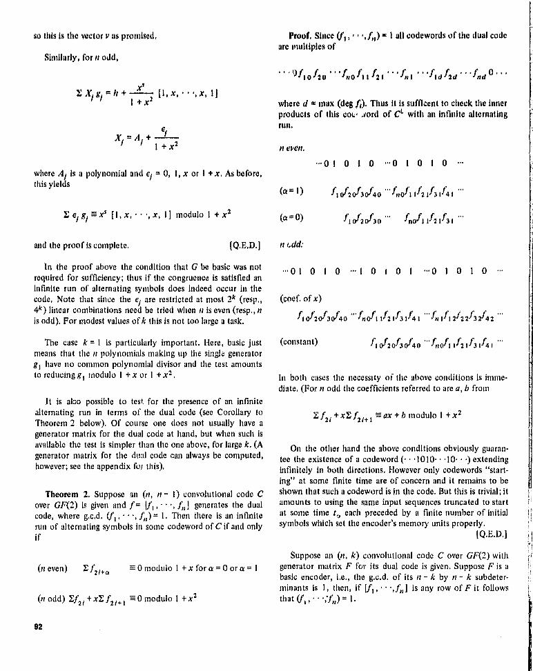
so this Is the vector v as promised, Proof. Since (fl , , f„) I all codewords of the dual codeare Multiples of
Similarly, for it odd,
X2: X/
gI =lr+ x1 +x2
[1,x,.. " x, IJ
X=A+ Et
1 +X2
where Al is a polynomial and el = 0, 1, x or I +x. As before,this yields
E ct g, = x` [ 1, x, • • , x, I ] modulo l + x2
mid the proof is complete. [Q.E.D.]
In the proof above the condition that G be basic was notrequired for sufficiency; thus if the congruence is satisfied aninfinite run of alternating symbols does indeed occur in thecode, Dote that since the et are restricted at most 2 k (resp.,0) linear combinations need be tried when it even (resp., itis odd). For modest values of k this is not too large a task.
The case k = I is particularly important. Mere, basic justmeans that the it polynomials making up the sft:ac generatorg i have no common polynomial divisor and the test amountsto reducing g 1 modulo I + x or 1 + x2.
It is aloo possible to test for the presence of an infinitealternating run in terms of the dual code (see Corollary toTheorem 2 below). Of course one does not usually have agenerator matrix for the dual code at hand, but when such isavailable the test is simpler than the one above, for large k. (Agenerator matrix for the dual code can always be computed,however; see the appendix for this).
Theorem 2. Suppose an (n, it - 1) convolutional code Cover GF(2) is given and f = (J I , • • •, J;,] generates the dualcode, where g.c.d. (f I , • • •, f„) = 1. Then there is an infiniterun of alternating symbols in some codeword of C if and onlyif
(►t even) E f2 0 modulo I + x for a = 0 or a = 1
(it odd) Ef2t + xE J2 t,} I = 0 modulo I +X2
. . ,Oflo f20 ... fnO flI f2l ...41 ... f1a f2d ... fnd0...
where d = max (deg ft). Titus it is sufficent to check the innerproducts of this co y• .vord of CL with an infinite alternatingrun.
it even.
^• 0 1 0 1 0 ... 0 1 0 1 0 •••
(Ci =1) f10f20f30f40 •••fit0fl1f2lf31fa1 •..
(a=0) f10t20f30 fnOfllf Al .+
it
••• 01 0 1 0 ••• 1 0 1 0 1 ••• 0 1 0 1 0 •••
(coef. of x)
fl A A A0 ... fn0' 1 lf2lf3 ifa 1 ..,fn If12/22f32fa2 ...
(constant) fl A A 044 0 ...fnofl If2l f31 441 ...
In both cases the necessity of the above conditions is imme-diate. (For it odd the coefficients referred to are a, b from
Tf21+xEf2t+l -ax+b modulo 1 +x2
Oil other hand the above conditions obviously guaran-tee the existence of a codeword (• • • 1010• • • 10• • •) extendinginfinitely in both directions. However only codewords "start-ing” at some finite time are of concern and it remains to beshown that such a codeword is in the code. But this is trivial; itamounts to using the same input sequences truncated to startat some time t. each preceded by a finite number of initialsymbols which set the encoder's memory units properly.
[Q.E.D.]
Suppose an (n, k) convolutional code C over GF(2) withgenerator matrix F for its dual code is given. Suppose F is abasic encoder, i.e., the g.c.d. of its it - k by it - k subdeter-minants is 1, then, if UI , •, J;, ] is any row of F it followsthat ((t , ...,'f„) = 1.
92

Let C, (i - 1, - - •, it - k) be the (►l, n - 1) convolutional codedual to the ith row of F. Clearly
C contains an infinite run of alternating symbols then themaximum run of alternating symbols in any codeword of Chas length L = s + n - 2 when n is ( , 7r-n or when n is odd and
n-k
c n C,r= l
and the maximum run of alternating symbols n any codewordof C has length L = L(C) < min L(Q,
Corollary. When n is odd an (►r, k) convolutional code Cover GF(2) contains a codeword with an infinite run of alter-nating symbols if and only if every row of a basic generatormatrix F for CL satisfies the congruences of Theorem 2. Whenn is even it is further necessary that this be true for the samevalue of a (0 or 1).
Note. Suppose n is even and L(CI) = L(Cl) _ - with a 0 1for C, and a :* 0 for Ci . Add row f to row 1 i F; this gives anequivalent basic encoder which has L(Ci) < -.
III. Bounds For Finite Runs of AlternatingSymbols
If no codeword contains an infinite run of alternatingsymbols the question arises as to the maximum length L ofsuch a finite run. It is easy to give a bound for L in terms ofthe generators for the dual code. From this bound it is possibleto derive another bound (in general, weaker) which has theadvantage that it can be applied directly without knowledge ofthe dual (see the Corollary to Theorem 3, below). In Section 4these bounds are applied to some specific examples.
Suppose [fl , - - j;,] is a generator matrix for an (n, 1)convolutional code C over GF(2) with d = max (deg fj), then
f1of20 . ' . fit A If2I ' ' ' fn - - * flAd ... find
is its associated bit pattern. Let s be the number of symbolsoccurring between the first and last nonzero symbols fjj inclu-sively. If (fl , - - -, fn ) = 1, s is the minimum length of anynonzero codeword of Cand
n(d- 1) + 2 < s < n(d + 1)
Theorem 3. Let C be an (n, n - 1) convolutional code overGF(2) with generator matrix for its dual code given by
V1 , - - -,fn], where (fl , - - -,f,,) = 1. Suppose no codeword of
h(x) = E f2i + x E f2t+l E I + x modulo 1 + x2
If it is odd and h(x) = I or x modulo 1 +x2 the maximum runof alternating symbols has length L = s + 2n - 2.
Combining this with the limits given above fe, s yields
nd n(d + 2) - 2 n even or n odd,h(x) = 1 + x
<L <
n(d + 1) n(d + 3) - 2 n odd, h(x)1 or x
Proof. S l ippose n is even. Then from Theorem 2 aboveE f2i = 1 f2i+l = 1 modulo 1 +x. If there were an alternatingrun of length > s + n - 1 it would have s consecutive symbolswhich would have inner product zero with the bit pattern ofthe f's. This contradicts E f2 i ° E f2 t+ 1 E 1, so L < s + n - 2.On the other hand consider an alternating run of length s + n.Change the first and last of these symbols; the inner productswill be correct provided that they match up with the symbols1, , , • , s and it 1, - • - , n + s. Clearly this run can beextended to the right and the left to form a codeword of C; itis merely a matter of selecting symbols I ± in so that the innerproducts are zero. Such a codeword could conceivably extendinfinitely in both directions; however using the same argumentas at the end of Theorem 2 it follows that there is a finitecodeword with an alternating run of this length.
If it odd then, from Theorem 2, h(x) EO 0 modulo 1 + x.2.
If h(x) = 1 + x the proof above applies, so L = s + it - 2. Ifh(x) = 1 or x then one of the inner products is zero but theother is not (see the display shown in the proof of Theo-rem 2). If there were a run of length > s + 2n - I there wouldhave to be a run of s consecutive symbols where the innerproduct was zero. Oil side or the other of these s symbolsthere would have to be it symbols from the alternatingrun of size s + 2n - 1. These it symbols together with s - it
the original s symbols would also have to have inner productzero contrary to the hypothesis,
So L < s + 2n - 2. As above a finite codeword of C can beconstructed containing an alternating run of length L = s + 2n- 2. It is merely necessary that positions n, • • - , it + s - 1 ofthis run have inner product zero with the bit pattern of the f's.
[Q.E.D.]
93

Recall from the previous section the codes C, ]( ►r, it - I )convolutional codes dual to the rows of F, where F was it basicgenerator matrix for CL ] and the obvious property
n-k
C= (1 c,► = t
front which it follows that the maximum run of alternatingsymbols in any codeword of C has length L = L(C) < ►nirL(Cj). Suppose L(CI) is finite for at least one value of i. Thenif d is the maximum degree of any element in the i ll' row of Fit follows that
n(d + 2) - 2 n even
L(C) < L(C,) 6
n(d + 3) - 2 it odd
Corollary. Suppose an (n, k) convolutional code C overGF(2) is given with ba.i., generator matrix G. Let p be themaximum degree of the k X k subdeterminants of G. Theneither L = L(C) = - or
n(p + 2) - 2 it even
L ^
n(p + 3) - 2 it odd
Proof. Under these conditions Cl has a generator matrix F(a so-called minimal encoder for CI) all of whose entries are ofdegree < p. Thus the result follows immediately except whenit even and L(Q _ — for 1 = 1, - - , , it k. Here if L is finite,a finite bound for it can be determined by replacing row 1 of Fin turn by the sum of row i and row j, for% 1, • • -, it - k 00i). Of course, in general, all this work will not be required butthe point is that such transformations do not increase themaximum degree of the elements of the dual encoder and sothe bound given above is valid here also.
IV. Some ExamplesConsider the (3, 2) code C generated by the encoder G
0 x+I x+1
(mod I + x2)
1 I x
Note that the sum of its rows is congruent to 11, x, I ] modulo1 + x2 thus, by Theorem 1, C contains a codeword with aninfinite run of alternating symbols. As mentioned in Section 2this conclusion is valid even though G is not a basic encoder (x+ x 2 divides Its 2 X 2 subdetertninants). Applying Theorem 2to the dual encoder F= [xs +x3 +x 2 +X, x 3 +X 2 + 1,x4 +X+ I] note that (ft , f2 , f3 ) = 1 and that f2 + Xf► +xf3 =X 6 +X 5 + X4 + x2 + x + I = 0 modulo 1 + x2 so that again theexistence of a codeword in C with all run of alternat-ing symbols is assured. Cl does not contain such a codewordsince Fis a basic encoder and F= [1 +x, x, x] modulo 1 +X2.
As a second example consider the (4, 1) code C withgenerator F' of its dual code given by
X x3+X+1 x+1 x2+x+I
X 2 +X + 1 X3 + ] X3 X2 + 1
x 2 X2 +X + 1 x2 X3 + l
I 1 0 1 a=0
1 0 1 0 a = 0, 1
1 1 1 0 Ja = I
Thus each row of F' satisfies the congruences of Theorem 2for some value of a. But row 1 satisfies the congruence onlyfor a = 0 and row 3 only for a = 1. Thus C does not contain acodeword with an infinite run of alternating symbols. In factsince the sum of rows 1 and 3 of F' has degree d = 3 it followsthat the maximum run of alternating symbols in any codewordof C is bounded above by n(d + 2) -2 = 18. A basic generatorfor Cis [I +x2 +X4 +x 5 +X6 +X7 +x8,X3 +x4 +XS + X9,x+X7 +X8 ,X +X2 +x3 +X 6 +X7 +XS +X9] thus µ = 9 andthe Corollary to Theorem 3 gives only the weaker bound n(p +2) 2 = /,2.
Up to this point the distinction (mentioned in the appen-x3 + x x3 + 1 X4 +X 2 + x + 1 dix) between the dual generators F and F' has been over-
___ looked. Actually it is F' that is used in the proofs of Theo-rems 2 and 3. There is no problem with this because either F
X 2 X3 + x + l x3 +X2 + 1 and F' both satisfy the congruences of Theorem 2 or they
sa
0PAGU TY
11,1 p^ . QUA LI
OF,

both do not, Similarly in Theorem 3 h(x) La I +x for Fif andonly if h(x) s I + x for F'. However if the actual value of s isto be used to establish a bound the bit patterns of F'should beexamined as s can differ for corresponding rows of F and F'.In the case at stand the sum of rows 1 and 3 of F' has s = 14;soLSs+n - 2 = 16.
So if X4 = 1 + x2 + x3 (= 10110 . . .) and X2 = X + x2 +X3 +X4 with X i = X3 = 0, the codeword generated by G is
00011111 01010101 01010101 01010101 010111...
In the example above the Corollary to Theorem 3 was alittle disappointing in that it gave a bound of 42 whereas morecareful examination yielded L < 16. (Even 16 may be teohigh; a cursory examination of the bit p0tern associated withthe basic generator for C given above indicates that 13 may bethe answer). When k = it 1 it is clear from Theorem 3 thatencoders do exist for which the bound given by the Corollaryis tight, In general there are minimal encoders whose codeshave no infinite alternating run but do possess codewords withfinite alternating runs of length tip + k + 1 which comparesreasonably well with the bounds given by the Corollary. E.g.,consider the (it, k) convolutional encoder
I 0'
G =-
0 ... 0 pgpq..
where I is an identity matrix of order k - 1 and 0' is a k - 1 byit - k + 1 matrix of zeros.
Here p = p(x) = 1 +x +xµ and for n even q = q(x) = I +x2+ xt' (µ > 3) while for it odd q(x) = 1 + x 3 + xµ (p > 4). G isobviously basic and minimal. Further Theorem I guaranteesthat no codeword generated by G contains an infinite run ofalternating symbols. That G generates a codeword with a runof alternating symbols of length tip + k + 1 can be confirmedby selecting the inputs X t , • • • ,Xk properly. E.g., let it = 8, k= 4 and p = 3 then the bit pattern associated with the bottomrow of G is
00011111 00010101 00001010 00011111
which starting with Its 8th symbol has an alternating run oflength 29 = 8 - 3 + 5. Obviously X, , - ' - , Xk- i can always beadjusted tn fill in the first k - I symbols of each block of itsymbols in the proper fashion. So the Input Xk is the criticalone. For n even, k even and p odd Xk = I + x2 + x4 + • . . +xµ- I + xu . Similar formulas exist for the other cases-when it isodd these vary with p modulo 4,
As final examples consider the NASA Planetary Standardencoders of rates 1/2 and 113 (Ref. 3). Here G = 1911 921 orf91 192,931 With g, = I +x 2 +x 3 +xs +x6 , 92 = 1 tx tx 2 +X3 + x6 , 93 = 1 + x + x 2 + x4 + x6 . Then both are basicminimal encoders which do not possess infinite alternatingruns in any codeword as Theorem I easily shows. (Note that[9 1 , 93 , 921 and 1921 93, 9t do possess such runs, thus ifinfinite alternating runs are to be avoided the outputs in [gt,92 , 931 must be interleaved properly). For the rate 1/2 codethe Corollary of Theorem 3 yields L < 2 - 8 - 2 = 14 andTlicorcin 3 itself guarantees the existence of finite codewordswith alternating runs of this length, since s = 14 in this case.The rate 1/3 code has a dual generator F' given by
X 1 +x 2 +x 3 1 +x +x2 +x3 h(x) = 1 +x
F'
I +x 3x31 +x+x2h(x) =0
Apply Theorem 3 to the first row of F. Here s = 1 I so L < s +n - 2 = 12. A finite codeword with an alternating run of length12 is generated from G by tine input X i = 1 +x +x 2 +x4 +x7(_ • • • 01 11010010 . • •); so this bound is achieved.
95

Appendix
Convolutional Encoders
Proofs of most of the results mentioned here may be foundin Forney (Ref. 1). Computations are restricted to GF(2);however everything is easily generalized to any finite field.
A k X it G of polynomials gil determines a rate k/n(k < n) ennvolutional encoder with input sequences X! (i =1, - • - , k) and output sequences Yl Q = 1, - • -, n), where
kYI Xi gil
provided that G is of rank k. These output sequences Yl areinterleaved to produce a single codeword
Yll 21 ' ' * r.i 12 22..
n2 ...
The collection of all such codewords (.e., the "rov space" ofG) Is the rate k/n convolutional code generated by G. Such anencoder may be realized by k shift registers the ith of whichcontains vi memory units where vi = maxl(deg gil); vi is calledthe constraint length of the ith register. This is said to be theobvious realization of the encoder G and thus requires v = E vimemory units in all (v is the overall constraint length of therealization).
Two convolutional encoders are equivalent if they generatethe same code. An encoder is called basic if there is nopolynomial it (deg It a 1) which divides all the k X k subdeter-minants of G. Basic encoders do not suffer from catastrophicerror propagation and thus they are preferred over others.Fortunately every code can be generated by some basicencoder, Le., there exists a basic encoder equivalent to anygiven encoder G.
In general a basic encoder that has maximum degree pamong its k X k subdeterminants requires at least µ memoryunits for its implementation. Sometimes it requires more.When µ is obviously sufficient, i.e, when µ = E vi , the encoderis said to be a minimal encoder. Since equivalent basicencoders have the same value of µ, a minimal encoder requiresas few memory units as any equivalent basic encoder. In fact, aminimal encoder requires as few memory units as any equiva-lent encoder, basic or not. Again, every encoder is equivalentto some minimal encoder. So, theoretically at least, there is noloss in assuming that any particular code at hand is generated
by a minimal encoder. (Finding a minimal encoder equivalentto a given encoder can be a computational chore however; seebelow). It is a direct consequence of the minimality conditionthat any linear combination of the generators of a minimalconvolutional encoder has degree greater than or equal to thedegrees of all the generators occurring in the combination.This implies that equivalent minimal encoders not only havethe same overall constraint length v = E vi , but that they alsohave the same number of generators of each degree. Le., theset of degrees vi (i = 1, - - • , k with multiplicities counted) isan invariant of minimal encoders under equivalence. Closelyrelated to these last two comments Is a property of minimalencoders called the predictable degree property which allowseasy ennumeration of the short codewords generated by aminimal encoder, see Ref. 1.
Associated with any (n, k) convolutional code C is its dualcode 6. CL is the (n, n - k) convolutional code which consistsof all sequences orthogonal to every codeword of C. If C isgenerated by a minimal encoder with overall constraint lengthv then CL can also be generated by a minimal encoder of thesame overall constraint length.
If [g i , , • •, gn ] is a generator matrix for the (n, 1)code C and if Efigi = 0 for polynomials fl , • • -, f, it isalgebraically convenient to consider V1 ,, - • • ,f] as a row of agenerator matrix F for C L . But if one considers the codewordsthe coefficients of the ft's must be reversed. For example, let it= 2; then one codeword of C is
.. . 0g io g20 giI g2i g i2 g22 .. .
This codeword is orthogonal to the symbol sequences
... flof2o0... R=0
... fllf2ifiof2o0-•• Q=1
since the respective inner products are the coefficient of x 2 in
Efigi = 0. Thus each f in F should be replaced by xa f(1 /x)where a is the maximum degree of any element of F. An
96

equivalent generator matrix F' is given by x'' ► f( U.0 where vi isthe maximum degree of any clement in row i of E If F is aminimal encoder then so is F'. The sequence (vi ) of maximumdegrees of cite rows is the same for F and F', thus they havethe saute overall constraint length also. Thus for most purposesF call be taken to be the generator matrix of the dual code Cl.
Every generator matrix G has all factor Jecompo.sition G - AI'B. Here A and B are square matrices of deter-minant I with polynomial elements. A is k X k and B is it X n,Pis a k X it diagonal matrix whose diagonal elements yr (I =I, • - -, k) are nonzero polynomials. The y 1 are called theinvariant factors of G and yr divides yi , t . Over GF(2) anencoder is basic if and only if yk = 1. This decomposition of Gcall produced by elementary row and column operations oilG; see, for example, Gantmacher (Ref. 2). Now the first krows of B constitute a basic encoder equivalent to G. Further-more B- n exists and has polynomial elements. If FT denotesthe last it k cctlunuts of ,B- t , then F is a n- k X npolynomial matrix which is a basic encoder for the dual codeCL.
Thus given any encoder G it is possible to find an equiva-lent basic encoder by computing the invariant factor decompo-sition. However simpler methods often suffice. If G is notbasic, i.e., if the greatest common divisor of the k X ksubdeterminants of G is a polynomial h of degree > I, let 0 beany irreducible polynomial dividing h. Then some linear conyb;nation of the rows of G is divisible by ^. By performing arow reduction of G modulo tG one determines a transforma-tion matrix T of determinant 1 such that TG has a rowdivisible by ;P. Divide this row by 0; this produces an encoder
equivalent to G with h replaced by hl/ . Eventually thisprocess terminates in all equivalent to G with h = Ii.e., all basic encoder.
Similarly, if G Is basic but not minimal the matrix of p;n ► 'order terms of G will have rank less than k, thus a rowreduction of this matrix leads to a transformation 7' of deter-minant I such that TG has smaller overall constraint lengththan G. Clearly, after at most L pi - N of these steps a minimalencoder equivalent to G will be produced.
An alternate method of finding generators for the dual codealso exists. After all, any it - k linearly independent vectorsorthogonal to G will form such a generator matrix, so thefollowing process can be used to produce them one at a time.Suppose an (n, k) encoder G is given. Since G has rank k somek X k subdeternninant is not zero. Let H be the matrix formedfrom these k columns plus one other. Then H has dimension kX k + I and is of rank k. Consider the k + I X k + I matrix II'whose first k rows are H and whose k + 1 51 row is row I of H.Expanding IH'I in terms of this last row shows that the vectorof cofactors is orthogonal to every row of H, since IH'1 = 0.Thus using this vector of cofactors to specify k + I compo-nents and setting the other components equal to zero we havea generator for Cite dual, Adjoin this generator to G and repeatthe process until it - k generators have been found. These itk generators will generate the dual code. Note that after j rowshave been added to G it will have rank k + j so the processdoes not break down. Further, in the special case where k = it- 1, the single generator for the dual code will be basic if Gwas. (In general this will not be the case for k < it - Ihowever).
Acknowledgement
The authors wish to thank M. K. Simon and J. G. Smith for bringing this problem totheir attention and for suggesting several possible approaches.
References
1. G. D. Forney, Jr., "Convolutional Codes 1: Algebraic Structure", IEEE Trans. Inform.77reory, Vol !T -16, November 1970, pp. 720 .738 (See also correction: same journal,May 1971, page 360).
2. F. R. Gantmacher, The 77reory of Matr ces, Chelsea, New York, 1959.
3. NASA Planetary Program Flight/Ground Data Systenv Standards. Revision 5, Jime 1,1977. National Aeronautics and Space Administration, Washington, D.C.
97
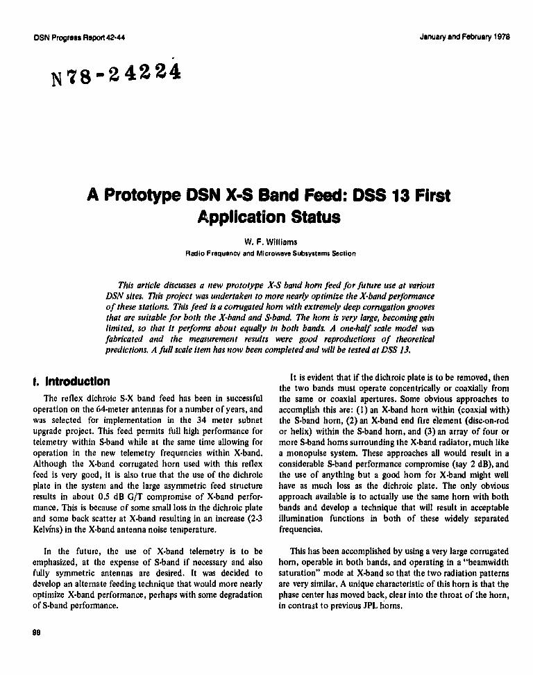
DSN Progress Report 42.44
January and February 1978
NP1g-24224
A Prototype DSN X-S Band Feed: DSS 13 FirstApplication Status
W. F. WilliamsRadio Frequency and Microwave Subsystems Section
This article discusses a new prototype X-S band horn feed for future use at variousDSN sites. This project was undertaken to more nearly optimize the X band performanceof these stations. This feed is a corrugated horn with extremely deep corrugation groovesthat are suitable for both the X-band and S-band. The hom is very large, becoming gainlimited, so that It performs about equally in both bands. A one-half scale model wasfabricated and the measurement results were good reproductions of theoreticalpredictions. A full scale item has now been completed and will be tested at DSS 13.
i. IntroductionThe reflex dichroic S-X band feed has been in successful
operation on the 64-meter antennas for a number of years, andwas selected for implementation in the 34 meter subnetupgrade project. This feed permits full high performance fortelemetry within S-band while at the same time allowing foroperation in the new telemetry frequencies within X-band.Although the X-band corrugated horn used with this reflexfeed is very good, it is also true that the use of the dichroicplate in the system and the large asymmetric feed structureresults in about 0.5 dB G/T compromise of X-band perfor-mance. This is because of some small loss in the dichroic plateand some back scatter at X-band resulting in an increase (2-3Kelvins) in the X-band antenna noise temperature.
In the future, the use of X-band telemetry is to beemphasized, at the expense of S-band if necessary and alsofully symmetric antennas are desired. It was decided todevelop an alternate feeding technique that would more nearlyoptimize X-band performance, perhaps with some degradationof S-band performance.
It is evident that if the dichroic plate is to be removed, thenthe two bands must operate concentrically or coaxially fromthe same or coaxial apertures. Some obvious approaches toaccomplish this are: (1) an X-band horn within (coaxial with)the S-band horn, (2) an X-band end fire element (disc-on-rodor helix) within the S-band horn, and (3) an array of four ormore S-band horns surrounding the X-band radiator, much likea monopulse system. These approaches all would result in aconsiderable S-band performance compromise (say 2 dB), andthe use of anything but a good horn for X-band might wellhave as much loss as the dichroic plate. The only obviousapproach available is to actually use the same horn with bothbands and develop a technique that will result in acceptableillumination functions in both of these widely separatedfrequencies.
This has been accomplished by using a very large corrugatedhorn, operable in both bands, and operating in a "beamwidthsaturation" mode at X•band so that the two radiation patternsare very similar. A unique characteristic of this horn is that thephase center has moved back, clear into the throat of the horn,in contrast to previous JPL horns.
98
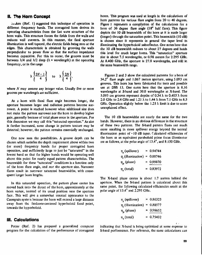
II. n1 o Hom Concept
aZaken (Ref. 1) suggested this technique of operation indifferent frequency bands. The corrugated horn derives itsoperating characteristics from the fast wave structure of thehorn walls. This structure forces the flews front the walls andreduces wall currents. In this manner, the final apertureillumination is well tapered, the electric fields being zero at theedges. This characteristic is obtained by grooving the wallsperpendicular to power flow so that the surface impedancebecomes capacitive, For this to occur, the grooves must bebetween X/4 and X/2 deep (X - wavelength) at the operatingfrequency, or in the range
1
2N- I I to X 2N4 4 '
where N may assume any integer value. Usually five or moregrooves per wavelength are sufficient.
As a horn with fixed flare angle becomes longer, theaperture becomes larger and radiation patterns become nar-rower, A point is reached however when additional size doesnot make the pattern narrower nor the horn to develop highergain, generally because of total phase error in the aperture. Forthis discussion we may call this "saturated operation," As sizeis further increased, some change in pattern texture may bedetected; however, the pattern remains essentially unchanged.
One now sees the possibilities. A groove depth can bechosen which satisfies the depth requirement above within two(or more) frequency bands for proper corrugated hornoperation, and sufficiently large to just be "saturated" in thelowest band so that the higher bands would be operating wellabove this point for nearly equal pattern characteristics. Thebeamwidth for these "saturated" conditions is a function onlyof the horn flare angle, and not the aperture size. Narrowerflares result in narrower saturated beamwidths, with conse-quent longer horn lengths.
In this saturated operation, the pattern phase center hasmoved back into the throat of the horn, approximately at thehorn vertex, instead of its usual position near the apertureface. This will give a somewhat unusual appearance to theCassegrain syste • n because the horn will extend a large distanceaway from the feedcone-centered hyperboloid focal point,towards the hyperboloid.
III. Calculations
horns. This program was used at length in the calculations ofhorn patterns for various flare angles from 20 to 40 degrees.Figure i represents a compilation of the calculations for ahorn of 36 degree flare angle (I r half flare). This figuredepicts the 10 dB beantwidth of the horn as it is made larger(longer) through the saturation point. This bearnwidth (10 dB)Is chosen since it represents in general the taper level inilluminating the hyperboloid subreflector. One notes here thatthe 10 dB beamwidth reduces to about 27 degrees and holdsthis level for much larger horns, This "saturation" aperturesize is about 7.5 wavelengths, or 0.98 meters for 2.295 GHz.At 8.400 GHz, the aperture Is 27.8 wavelengths, and still inthe same beamwidth range.
Figures 2 and 3 show the calculated patterns for a horn of34,2 0 flare angle and 1.067 meters aperture, using 5.093 cmgrooves. This horn has been fabricated for tests and possibleuse at DSS 13. One notes here that the aperture Is 8.16wavelengths at S-band and 30,0 wavelengths at X-band. The5.093 cnt grooves represent depths of 0.34 X to 0.403 X from2.0 GHz to 2.4 GHz and 1.21 X to 1.44 X from 7.1 GHz to 8,5GHz. Operation slightly below the 1.25 X limit is due to someunexplained effect.
The 10 dB beamwidths are nearly the same for tite twobands. However, there is an obvious difference in the structureof these two patterns. The S-band pattern flares out muchmore resulting in more spillover energy beyond the normalillumination point of -10 dB taper. !'alculated efficiencies ofthe horn as an equivalent paraboloid prime focus illumin;itorare as follows, at the polar angle of 13,4 0 , and 8.150 GHz,
ri,, (spillover) = 0.94744
rtr (illumination) = 0,88746
77 (phase) = 0.99870
tl l (total) = 0.83972
The X-band phase center is about 1.7 meters behind theaperture. When the S-band pattern is calculated about thissame point, the following calculated efficiencies result at thepolar angle of 13.4 0 and 2.295 GHz.
ns (spillover) = 0.86323
of (illumination) = 0.88577
rip (phase) = 0.98652
rlr (total) = 0.75432
Potter (Ref. 2) has prepared a generalized computer indicating that X-band is being optimized at some expense to
program for the calculation of the performance of corrugated S-band performance. For reference, the same calculations can
99

be made using the present DSN corrugated horns as used in anequivalent paraboloid system. Those results are:
n, (spillover) = 091454ni (illumination) = 0,89114tip (phase) = 0.99836
nr (total) = 0.8^ 1365
This shows the new feed, as applied in a conventionalparaboloid/hyperboloid system gaits 2.6% at X-band andlosses 5.9% at Shand, as a direct substitute.
Probably one of the most valuable and unexpected resultsfrom this type of horn is the complete lack of any sort ofsidelobe. Note that the level scale is for a 60 dB range, and atX-band the main lobe reduces to this level and does notreappear. This makes the horn very attractive in the proposeddual reflector antenna shaping applications since it willimprove spillover efficiency even more and possibly aid in thefurther reduction of total antenna noise.
IV. The Hag Beane Model
Figure 4 is a photograph of the one half scale model thatwas constructed and measured during this development, Thismodel had a 34.2° flare angle, a 53.34 cm aperture, and 2.548cm grooves. Measurements were then made throughout theappropriate frequencies to verify predicted performance.Figures 5 and 6 are these measured patterns at two frequen-cies, 16 .3 CHz and 4 .4 CHz. These measurements indicate anexcellent agreement with theory. The 10 d6 beamwidths areabout the same and as expected, sidelobes do not exist.
A full scale version is being constructed for tests andpossible other uses at DSS 13, such as VLBI. Figure 7 depictsthis installation at DSS 13, indicating the relative hornpositions. This figure indicates, as was mentioned above, thatthe new X -S horn will extend much farther toward thehyperboloid from its feed cone location than the presentinstallation.
References
1. E. J. Jeuken and V. J. Vokurka, "Multi-Frequency Band Corrugated Conical HornAntenna," 1973 European Microwave Conference Proceedings, Vol. 2, Sept. 4-7,1973, Brussels University, Brussels, Belgium.
2. P. D. Potter, "Efficient Antenna Systems: A New Computer Program for the Designand Analysis of High Performance Conical Feedhorns," JPL Technical Report32. 1526, Vol. XIII, pp. 92. 107, Feb. 15, 1973.
100
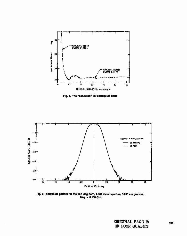
i40— I
I GROOVE DEPTHEQUAL 0.340 )+
35 - II
30 , GROOVE DEPTHEQUAL 1.3191.
0 10 20 30 40 50 60
APERTURE DIAMETER, wovolongtlr
Fig. 1. The "astursted" 38' corrugated hom
0
-10
AZIMUTH ANGLE - 0-20 (E THETA)
(E PHI)
-30W
r-5WK
-50
-60-80 -60 -40 -20 0 20 40 60 80
POLAR ANGLE, dog
Fig. 2. Amplitude pattem for the 17.1 deg hom, 1.087 meter aperture, 8.093 cm grooves,freq.. 8.160 0Hs
I
3
n
ORIGINAL PAGE lb 101OF POOR QUALITY

S
►OLAS ANGLE, dell
Fig. 3. Amplitude patlem for the 17.1 deg horn, 1.067 mater aperture, 5 063 cm grooves,". - 2.200 rjHz
10
vr
20
1
SW
N
4C
120 v0 60 30 0 30 60 90 120
ANGLE, dell
Fig. 4. The he" scale modal
Fig. S. Aftesured pattern of a (34.2)17.1 deg horn, 59.34 cmaperture, 2.546 cm grooves, freq. - 16.3 GMt M-plans
102

AN EXIS'S-BANS.
EXISTINGFEED CONE
HYPERSOLOIDFOCUS WITHIN
- • -W X-sORN
EXISTING FEEDCONE PLUS NEWEXTENSION
la
20
SWas
40
120 90 60 30 0 30 60 90 120ANGLE, dog
Fig, 8. Measured pattern of a (34.2)17.1 dog horn, 53,34 cmaperture, 2.548 cm grooves, freq. = 4.400 DHa H•plans
5,791 m TOPARAbOLOIFOCUS
1,716m
5.182m
PARABOLOID VERTEX
Fig. 7. Comparison of DSS 131nslallations
103

DSN Progress Report 42.44
January and February 1978
N
LAASP 100-m Antenna Wind Perdormance StudiesR. Levy and M. S. Katow
DSN Engineering Section
Structural design procedures are described for the LAASP antenna system to meetperformance requirements under gravity and wind loading. A computational method isshown for the evaluation of performance in response to wind loading. Cumulativeprobability distribution curves for wind loading gain reductions for 100-m-diameterantennas are developed to compare a relatively heavy baseline reflector backup structurewith two lighter-weight stnnetures; all have equivalent, acceptable performance for gravityloading.
I. hitroductionDesign studies for the Large Antenna Station Project
(LAASP) paraboloidal antenna structures are undertaken toderive cost and performance tradeoffs associated with a num-ber of configuration alternatives. Both cost and performancecan be characterized by any of a number of quantitativemeasures, while configuration alternatives also are conceptu-ally limitless. Consequently, to expedite timely completion ofany study, some restrictions on the scope are essential. Never-theless, within a framework of practical and reasonable restric-tions, it is feasible to develop significant parametric studyinformation for a comprehensive range of antenna structuredesigns within a given diameter class.
Within the context of the present discussion, cost will bemeasured by the structure weight. It is well known that weightis an imperfect measure of structure cost when a wide varietyof configurations with diverse fabrication, material, and instal-lation requirements are contemplated. However, when alterna-tive configurations are similar in concept, structure weight is aconvenient and acceptable cost measure. Performance will be
measured by the antenna radio frequency (RF) gain reduction,which depends upon the structural deformations caused bygravity and wind loading.
Gravity loading, which is always present on antenna struc-tures, is deterministic and well understood. Wind loading isstatistical, and the assessment of related response is morecomplex. Depending upon the location, wind can have a sig-nificant effect upon performance. Other loadings such asthermal, shock, and earthquake are primarily stochastic, diffi-cult to quantify, and of relatively short duration. These load-ings can be treated as constraints on the design to maintainstructure integrity and survivability but are not included forevaluation of operating performance.
Configuration studies will be limited to be within oneparticular reflector class: The traditional structural format ofradial rib trusses braced by circumferential hoop ring trusses.Within this format class, nevertheless, there are many possiblevariations of the geometrical arrangement, such as proportions,numbers and spacing of trusses, and the configuration of theexternal supporting structures. Several of these variations are
104
examined early in the present study but, for brevity, thedesigns to be described here will include only the preferentialgeometry as previously developed.
Here the emphasis will be placed upon the relationshipsbetween weight and performance for wind loading. The calcu.lationai procedure and results obtained will be described for aproposed 100-m-diameter antenna reflector system Illustratedin Fig. 1. This system is intended to operate at the X-bandfrequency of 8.5 Gliz. Cumulative probability distributioncurves of gain reduction for wind loading will be shown forthree alternative reflector designs for this system. Thesedesigns have the same geometry and differ only in the crosssectional areas of the bars chosen for the reflector backupstructure. They represent a baseline design and two lightervariations with weight reductions of up to 3070, All threedesigns are constrained to have equivalent performance in theabsence of wind loading. The maximum gain reduction due togravity loading is less than 107o of the total gain reductionfrom all sources. Those consist of manufacturing and surfacealignment errors and subreflector and quadripod blockage.
II. Sources of Gain ReductionTable I is a summary of the sources of gain reduction that
have been considered for gravity or wind loading. Two cate-gories are identified; the deformation-type category includespathlength phase errors of the radiofrequency (RF) beam; thebeam-deformation-type category covers pointing misalignmentlosses of the main beam with respect to the target.
Referring to the table, backup structure contribution iscomputed with respect to the paraboloid that best fits thedeflected surface. Surface panel contributions are also con-sidered with respect to a best-fitting surface. The subreflectoroffsets are the axial and lateral mismatches of the subreflectorposition from the focal point of the best-fitting paraboloid.For computational purposes, these offsets can be converted toequivalent additional backup structure deformations (Ref. 1).For gravity loading, which is repeatable and calibratable, thesubreflector can be repositioned to the actual focal point, andthus the offsets produce no gain reduction. Subreflector stir-face deflections are another source of deformation-type losses.However, these will be disregarded because appropriate designcan make them small.
The wind speeds are represented by the conventional modelof a slowly varying, quasi-steady component and a super-imposed gust turbulence. Beam deviation error that resultsfrom the steady component of the wind speed is corrected bya programmed pattern search that removes these low-frequency pointing errors. We make a conservative assumption,however, that the pattern search is too slow to overcome the
gust effects, so that gust loading always produces gain reduc-lions through beam deviations. The pointing errors from grav-ity loading can be overcome by calibration that compensatesthe input command signal. The servo loop error occurs becausethe servo system is not fully effective in compensating for thehigher-frequency components of the gust disturbance toque.The ability of the servo system to compensate depends uponthe servo loop transfer function in conjunction with the windgust spectrum. Calculations for typical antenna systems showthat from 75% to 90% of the angular errors detected at theencoders can be removed by compensation. To be conserva-tive, calculations here assume compensation of only 75% ofthese error magnitudes.
Ill. Reflector Design Synthesisthe baseline reflector backup structure design was devel-
oped by an evolutionary process. Although the JPUDEAScomputer program (Ref. 2) was used as a pivotal design tool toperform analysis and optimization of member cross-sectionalarea selection, no software was available to optimize thegeometrical proportions for this structure. Consequently theseproportions were developed from a sequence of trial variationsof the geometry. The variations were tested by analysis andmember area redesign within the IDEAS program to assesstheir ultimate potential.
The ordinarily laborious and time-consuming task of pre-paring the extensive data card sets required for structuralcomputer analysis was expedited by a program that auto-matically generated these cards for each variation. This pro-grain almost all of the card images needed to describereflector backup structures of the conventional radial rib trussand rLcumferential hoop type of construction. The sequenceof trial geometry generation and subsequent testing entailsgeneration and processing of an extensive data bank; neverthe-less, it is executed rapidly. Furthermore, only a limitedamount of effort by the engineer is needed. His participation isrequired primarily for decision-making to guide the operationsand to select from among the many options available to him,with only a small requirement for time to be spent on clericaltasks.
"lie root mean square (rms) pathlength deviation of thereflector surface front best-fitting paraboloid was selectedas the performance measure for design evaluation. The goalwas to achieve a reasonable balance between response togravity loading and response to wind loading. For the gravityloading, the objective response was the average of the rmsvalues over the elevation angle range weighted by trackingmission probabilities (Ref. 3) associated with the elevationangles A criterion wind-loading case was established to repre-sent the condition of the antenna at the 60-deg elevation angle
105
with a rear wind at an ,arbitrary reference speed of 13.4 in/see(30 inph). Previous experience with similar antennas indicatedthat this wind orientation was likely to be the most severe.During all of the redesign Iterations, member area selectionswere subjected to constraints on stress and buckling for thegravity loading, for the criterion wind loading, and for addi-tional wind loadings that represented the most severe opera-tional wind (31,3 in/sec) and the survival wind (44.7 m/sec).
The geometry evolved for the baseline design resulted In anearly homologous response (Ref, 4) for gravity loading r td avery good surface rnas (0.69 min) for the criterion wind load-ing, Two lighter-weight variations of the basic design weredeveloped by permitting a degeneration of performance forthe criterion wind loading but at the same time retaining tilestress and buckling constraints for all loads and by invoking anew constraint that maintained the performance for the grav-ity loading. The weight of the backup structure and counter-weight for the baseline design was 1210 tons, and the lighterdesigns produced reductions of 200 and 335 tons with thewind criterion loading rms values of 0.86 mm and 0.93 mmrespectively.
The alidade comprises a much less complex analyticalmodel than the reflector. The few data cards required foranalysis and redesign were hand-generated. The final geometryalso entailed evolutionary proportioning to achieve a favorablearrangement. Analysis and member redesign were performedby the IDEAS program using an option invoked to maximizestiffness with respect to pointing accuracy for wind loading.Only one alidade design was developed, and this is used tosupport all three of the backup structures.
The alidade model was eventually converted for analysis bythe NASTRAN program (Ref. 5). This was done for the con-venience of having a direct output of specific internal rotationangles related to the servo loop wind gust error. The NAS-TRAIN program analysis included the bending stiffness of thealidade bars, which is presently not possible within the IDEASprogram. Nevertheless, responses from the two programsagreed closely, indicating that the bending rigidity is notsignificant.
IV. Computational Model for WindLoading Gain Reduction
A multidimensional four-component statistical model wasused for computation of gain reduction due to wind loading.The four random components were (1) V, the mean windspeed; (2) v, a superimposed gust turbulence; (3) AZ, theazimuth of the wind relative to the antenna pointing direction;(4) EL, the elevation of the antenna relative to the horizon.
The mean speed has slow variations that comprise periodiccomponents measured by hours or days, Statistics of tite meanspeed obtained for the same site (Goldstone, California) as theproposed 100-in antenna have been tabulated in Ref. 6.
The gust speed was described by the conventional model,which represents the gusts as gaussian, with zero mean andstandard deviation a,, proportional to the mean speed; e.g.,
a,, = CV (1)
The tabulated mean speeds are based upon observations ata 46-m (150-ft) height above ground. For convenience, themean speeds here are also considered at the same height.Estimating the surface drag coefficient at 0.006 for the pro-posed terrain and using the computed power law coefficientI speed variations with height equal to 0.1405 (Ref. 6), wefind C = 0.1533.
Gusts are the dynamic component of the wind speed.Spectral decompositions according to conventional models(Refs. 7, 8) show that the predominant fluctuations arecharacterized by periods in the order of several seconds tominutes. The natural frequency of the antenna-reflectorsystern of Fig. 1 will be at least I Hz for the slowest naturalmode. The response of such a system to both the meanspeed and the gust speed is essentially the same as for staticload application. Consequently the structural response can becomputed as a static response to total wind loading V where
V= V+v (2)
Wind tunnel test data on antenna reflector and alidadecomponents (Refs. 9, 10) were used to canvert from windspeeds to pressure loadings on the proposed reflector andalidade structures. Wind tunnel tests are a logical and reason-able basis for deriving the pressures and forces for the meancomponents of the wind speeds. Nevertheless, it is recog-nized that using the same type of conversion for gust effectsis a major assumption and simplification of this model. Thegust speeds actually have a three-dimensional spatial correla-tion for which theoretical models require further develop-ment. A possible approach to providing a better estimate ofthe gust loading is available through computer simulation(Ref. 11). However, it was estimated that the application ofthis approach would have entailed a major additional compu-tational effort and also more wind tunnel test data than iscurrently available. Nevertheless, despite the simplified repre-sentation for gust loading, the present work employs thesame formulation to compare alternative designs and shouldfurnish a reaso ►lable basis for comparison.
106
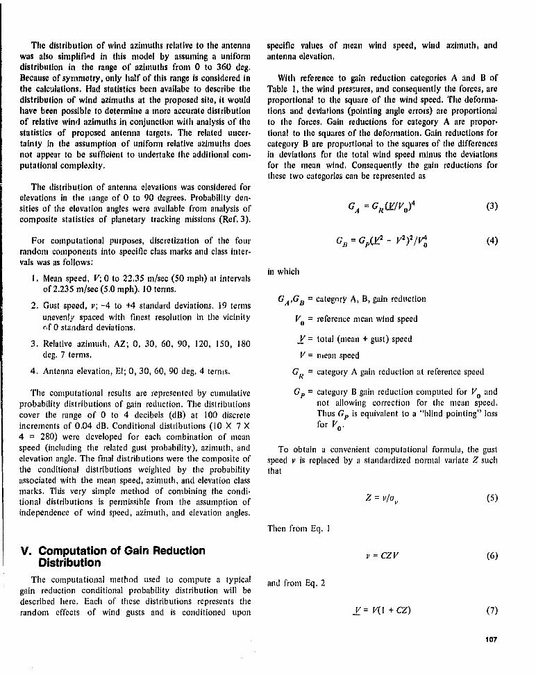
The distribution of wind azimuths relative to the antennawas also simplified in this model by assuming a uniformdistribution in the range of azimuths from 0 to 360 deg.Because of symmetry, only half of this range Is considered inthe calculations. [lad statistics been availabe to describe thedistribution of wind azimuths at the proposed site, it wouldhave been possible to determine a more accurate distributionof relative wind azimuths in conjunction with analysis of thestatistics of proposed antenna targets. The related uncer-tainty in the assumption of uniform relative azimuths doesnot appear to be sufficient to undertake the additional conn-putational complexity.
The distribution of antenna elevations was considered forelevations in the ► tinge of 0 to 90 degrees, Probability den-sities of the elevation angles were available from analysis ofcomposite statistics of planetary tracking missions (Ref. 3).
For computational purposes, discretization of the fourrandom components into specific class marks and class inter-vals was as follows:
I . Mean speed, V; 0 to 22.35 m/sec (50 ►npli) at intervalsof 2.235 in/see (5.0 mph). 10 terms.
2. Gust speed, v; '-4 to +4 standard deviations. 19 termsunevenly spaced with finest resolution in the vicinityr,f 0 standard deviations.
3. Relative azinnudi, AZ; 0, 30, 60, 90, 120, 150, 180deg. 7 terms.
4. Antenna elevation, El; 0, 30, 60, 90 deg. 4 terms.
The conputational results are represented by cumulativeprobability distributions of gain reduction. The distributionscover the range of 0 to 4 decibels (dB) at 100 discreteincrements of 0.04 dB. Conditional dist ributions (10 X 7 X4 = 280) were developed for each combination of meanspeed (including the related gust probability), azinnuth, andelevation angle. The final distributions were the composite ofthe conditional distributions weighted by the probabilityassociated with the mean speed, azinnuth, and elevation classmarks. Tlus very simple method of combining the condi-tional distributions is permissible from the assumption ofindependence of wind speed, azimuth, and elevation angles.
V. Computation of Gain ReductionDistribution
The computational method used to compute a typicalgain reduction conditional probability distribution will bedescribed here. Each of these distributions represents therandom effects of wind gusts and is conditioned upon
specific values of mean wind speed, wind azimuth, andantenna elevation.
With reference to gain reduction categories A and B ofTable 1, the wind pressures, and consequently the forces, areproportional to the square of the wind speed. The deforma-tions and deviations (pointing angle errors) are proportionalto the forces, Gain reductions for category A are propor-tional to the squares of the deformation. Gain reductions forcategory B are propurtional to the squares of the differencesin deviations for the total wind speed minus the deviationsfor the mean wind. Consequently the gain reductions forthese two categories call represented as
GA = GR (V/ Vo)4 (3)
GB = Gp(O - VZ )Z / a (4)
in which
GA ,GR = category A, B, gain reduction
Vo = reference mean wind speed
V = total (mean + gust) speed
V = niean speed
G = category A gain reduction at reference speed
GP = category B gain reduction computed for Vo andnot allowing correction for the mean speed.Thus Gp is equivalent to a "blind pointing" lossfor Vo.
To obtain a convenient computational formula, the gustspeed v is replaced by a standardized normal variate 7. suchthat
Z = ),/a t'(5)
Then from Eq. I
V = CZV (6)
and from Eq. 2
V = V(I + CZ) (7)
107

From these relationships, Eqs. 3 and 4 can be combinedso that the total gain reduction GT , which is the sum of GAand GR , call expressed as
bers of the alidade is also developed from wind tunnel data.For both reflector and alidade, sets of loads are developed tocorrespond with the discretization of wind azimuth andantenna elevation.
Gr = (GRfR + Gpfp) - wvo)4 (8)
where
fR = I + 4 CZ + 6(CZ)2 + 4(CZ)3 + (CZ)4(9)
fP = 4(CZ)' + 4(CZ)a + (CZ)4 (10)
The conditional distribution for gain redaction, F(GT),can then be obtained from Eq. 8, using the relationships ofEgs.9 and 10, Although the procedure is automated withina digital computer program, equivalent operations can beillustrated graphically with respect to Fig. 2 as follows,
Q
Compute GT for a set of values of Z in therange (-4, +4) and plot GT vs Z, as in Fig. 2a.
Q
As a selected value of gain reduction GTl , tutuintersections of GTr with the curve in QI .
0,® Project the intersections down to the curve inFig. 2b. Tlus curve is constructed to be thestaneiiard normal cumulative probability distribu-tion of Z. Read the ordinates where the projec-tions intersect the curve.
i^ The value of the distribution of gain reductionat GTr is the difference in the ordinates readfrom the curve of Fig. 2b,
A Computational ProcedureFigure 3 contains a schematic diagram of the complete
computational procedures used to derive the gain reductiondistribution for wind loading. The following notes apply totite labeled blocks of the figure:
Block 1. Wind tunnel pressure distribution data forspecific relative wind attitudes with respect to the antennaare converted to the force data required as input for reflec-tor analysis. The forces are represented by the three Carte-sian coordinates at each node and are derived from the inter-polated wind pressures, the surface area tributary to thenode, and the components of the unit vector normal to thesurface. Development of force data, except for the inter-polation, is automated. Wind loading on the structural menr
Block Z The reflector is analyzed by the IDEAS programto supply the responses to the wind loadings, The program isused here for analysis only, by specifying no redesign cycles.
Block 3. The alidade is analyzed by the NASTRAN pro.gram to find the response for the wind loadings. Wind reac-tions of the reflector on the alidade are included,
Block 4. Computation of pathlength deviations from thebest-fitting paraboloid are automated within IDEAS.
Block S. Gain reductions for subreflector offsets are cal-culated by hand, using results from the reflector analysis.
Block 6. Reflector contributions to the pointing errorsare automated within a separate computer program. Resultsare assembled within a matrix (4 elevations X 7 azimuths).
Block 7 Alidade contributions to pointing error and toservo loop are hand-computed (presently) and assembledwithin matrices.
Block 8. The category A (deformation-type) gain reduc-tions are combined by hand calculation. These individual G terms (Eq. 3) are assembled within a matrix.
Block 9. A compute program derives a matrix containingthe GP terms (Eq. 4). In the preceding blocks, the alidadeand reflector pointing deviations have been computed withseparate components for the elevation and cross-elevationaxes. Vector addition is required to combine the separatecomponents.
Block 10. The G. and GP matrices are input. A com-puter program develops conditional distributions for gainloss, described previously, for all 280 combinations of meanwind speed, wind azimuth, and antenna elevation,
Block 11. The computer program of Block 10 appliesprobability weighting factors for mean speed, wind azimuth,and antenna elevation to the conditional distributions andassembles the composite distribution of gain reduction forwind loading.
VII. Results and ConclusionsFigure 4 shows the distribution of gain reduction for
wind loading for the baseline 100-m antenna system and the
108

two alternative designs with lighter refle.tor backup struc.tures. As stated previously, all desivsis provide equivalenthigh performance for gravity loading.
average, the table shows this design to be only 0.04 dBworse than the baseline.
For ready reference, Fig. 4 tabulates reductions at a fewselected percentiles of 'he distribution. It can be noted, forexample, that ti,e reduction in weight of 335 tons for thelightest structure is achieved with a reduction in performanceof 0.37 dB (8% loss in efficiency) at the 98th percentile, andwith much smaller reduction at lower percentiles. On the
Whether or not the lightest design shown, or possibly adesign lighter than any of these, will be adopted must beconsidered in view of the performance requirements for theentire system. Tracking mission requirements and desiredreliability in conjunction with other sources of gain reduc-tion must be integrated within this type of evaluation.
References
1. Katow, M. S., "Evaluating Computed Distortions of Parabolic Reflectors," Mech-anical Engineering in Radar Symposium, Nov. 8-10, 1977, Washington D.C.
2. Levy, R., "Computer-Aided Design of Antenna Structures and Components," Com-puters and Structures, Vol. 6, pp. 419428, Pergamon Press, 1976.
3. Levy. R., "Antenna Bias Rigging for Performance Objective," Mechanical Engineer-ing in Radar Symposium, Nov. 8. 10, 1977, Washington D.C.
4. Von Hoerner, S. "Homologous Deformations of Tiltable Telescopes," J. StructDiv., Proc. ASCE 93(ST-5), Proc. Paper 5529, pp. 461.485.
5. Tile NASTRAN User's Manual, NASA SP-222(01), C. W. McCormick, editor, May1973.
6. Levy, R., and McGinness, H., Wind Power Prediction Models, JPL TM 33-802, JetPropulsion Laboratory, Pasadena, California, Nov. 1976.
7. Davenport, A. G., "The Spectrum of Horizontal Gustiness Near the Ground inHigh Winds," Quarterly Journal of tite Royal Meteorological Society, London, Vol.87, Aug. 1961, pp. 194-211.
8. Hino, M., "Spectrum of Guscy Wind," Pr.)ceedings of the Third Conference onWind Effects on Buildings and Structures, Tokyo, Japan, Sept. 6 . 11, 1971, pp.69-78.
9. Fox, N. L., Load Distributions on the Surface of Paraboloidal Reflector Antennas,Internal Memorandum JPL-CP 4, Jet Propulsion Laboratory, Pasadena, California,July 1962 (JPL internal document).
10.Blaylock, R. B., Aerodynamic Coefficients for "A Model of A Paraboloidal-Reflector, " Internal Memorandum JPL-CP6, Jet Propulsion Laboratory, Pasadena,California, May 1964 (JPL internal document).
11.Shinozuka, M. S., and Levy, R., "Digital Generation of Alongwind VelocityField," J. Engineering Mechanics Div., Proc. ASCE 103 (EM4), Proc. Paper 13159,Aug. 1977, pp. 689.700.
109

Table 1. Gravity and wind loading contributions togain reduction
Wind loadingGravitySource loading° Steady Gust
wind wind
A. Deformation typeBackup structuredeflection Contr Contr Contr
Surface paneldeflection Contr Contr Contr
Subreflectoroffsets Comp Contr Contr
B. Beam deviation typeBackup structurepointing error Calib Corr Contr
Alidade pointingerror Calib Corr Contr
Servo loop error None None Contr
aContr — Contributes to gain reductionComp — Compensated by subreflector repositioningCalib — Calibration used to modify the commanded positionCorr — Corrected by programmed pattern search
ORIGINAL; PAGE 15OP POOR +QUALITY
110

^l
c
t Mrp
r-
SIDE ELEVATION
REAR ELEVATION
Fig. 1. Configuration of 1004"larneter arden 11 system
JJ

2
2.0
^ 1.s
^ 1.0® G^
0.5 GTiz)
(a)GTaz(E90)
I1.0
U.
0.5—st
j F (GTi)I I
-4 -2 0 2 4
(b) CUMULATIVE (NORMAL)DISTRIBUTION OF z
Fig. 2. Development of cumulative distribution of Or
112

t 4
CONVERT WINDTUNNEL DATA TO RMS PATHLENGTH a t0STRUCTURE LOADING ANALYSIS
STATISTICAL ANALYSTSCOMBINE RMS OF GAIN REDUCTION2
PRATHSNOTHR
REFLECTOR LOADING CALCULATESUBREFLECTOR
CALCULATION LOOPSALL ELEVATIONS
RESPONSE ANALYSIS OFFSETS ALL AZIMUTHSALL STEADY SPEEDSGUST RANGE
CALCULATEREFLECTOR 9 11POINTING ERRORS
W PROBABILITY DISTRIBUTIONVECTOR OF GAIN REDUCTIONS 9 ADDITION
Z ALIDADE LOADING ALCALIDADE TE
32SRESPONSE ANALYSIS POINTING ERRORS
ZOPTIONAL RECYCLE
END
Fig. 3. Computational procedure
99.9BASELINE DESIGN
99 290 TONS LIGHTER98
ES335 TONS LIGHTER
90
r 6OFGAIN REDUCTIONS AT PERCENTILES
c OF DISTRIBUTION, dB
85% 90% 95% 98% AVG30 BASELINE .05 .09 .18 .53 108
O -200 T .07 .13 .29 .73 .101l -335 T .08 .14 .37 .90 .12
10
0.01r ,0.1 0.5 1.0 5.0
WIND LOADING GAIN REDUCTION, dB, AT 8.45 GHc
Fig. 4. Gain reduction for 100•m design variations
113

DSN Progress Report 42.44
January and February 1978
A Public-Key Cryptosystem Based On AlgebraicCoding Theory
R. J. McElieceCommunications Systems Research Section
Using the fact that a fast decoding algorithm exists for a general Goppa code, while nosuch exists for a general linear code, we construct a public-key cryptosystem whichappears quite secure while at the same time allowing extremely rapid data rates. This kindof cryptosystem is ideal for use in multi-user communication networks, such as thoseenvisioned by NASA for the distribution of space-acquired data
I. IntroductionRecently, Diffie and Hellman (Ref. 3) introduced the
notion of a public-key cryptosystem in which communicationsecurity is achieved without the need of periodic distributionof a secret key to the sender and receiver. This property makessuch systems ideal for use in multi-user communicationnetworks, such as those envisioned by NASA for the distribu-tion of space-acquired data (Ref. 4). Later, Rivest, Shamir andAdleman (Ref. 7) explicitly exhibited such a system, usingfacts from number theory, and Merkle and Diffie (Ref. 6)exhibited one based on the known difficulty of the integer-packing "knapsack" problem. In this paper we propose apublic key cryptosystem which is based on the theory ofalgebraic codes.
II. Description of the SystemWe base our system on the existence of Goppa codes. For
the full theory of such codes the reader is referred to (Ref. 5,Chapter 8), but here we summarize the needed facts.
Corresponding to each irreducible polynomial of degree tover GF(2'"), there exists a binary irreducible Goppa code oflength n = 2', dimension k> n - tm, capable of correctingany pattern of t or fewer errors. Moreover, there exists a fastalgorithm for decoding these codes. [Algorithm due toPatterson. See Ref. 5, problem 8.18. The running time iso(nt)] .
Suppose the system designer picks a desirable value of nand t, and then randomly selects an irreducible polynomial ofdegree t over GF(21"). Since the probability that a randomlychosen polynomial of degree t is irreducible is about l Jt, andsince there is a fast algorithm for testing irreducibility (seeRef. 1, Chapter 6), this selection would be easy to do. Next,the system designer produces a k X n generator matrix G forthe code, which could be in canonical, for example row-reduced echelon, form.
Having generated G, the system designer now "scrambles"G by selecting a random dense k X k nonsingular matrix S, anda random n X n permutation matrix P. He then computes
114

G'xSGP, which generates a linear code with the same rate andniinhmum distance as the code generated by G. We call G' thepublic generator matrix, since It will be made known to theoutside world.
The system designer then publishes the following dataencryption algorithm, which Is to be used by anyone desiringto communicate to film In a secure fashion,
Algorithm E
Lot the data to be encrypted be divided Into k•bit blocks. Ifu Is such a block, transmit the vector x = u G' + z, where G' isthe public generator matrix, and z is a locally generatedrandom vector of length n and weight t.
Having received x, the system designer can recoverefficiently by using the following decryption algorithm:
Algorithm D
Compute x' = xP" I , where P-1 is the Inverse of thepermutation matrix A x' will then be a codeword in theGoppa code previously chosin. Using Patterson's algorithm,one then computes u S = u'. Finally, u is computed byus=1.
III. Discussion
It Is clear that algorithms D and C can be Implementedquite simply. What remains to be studied Is the security of thesystem, What we need to determine, essentially, Is howdifficult it will be for an eavesdropper who knows G' andintercepts x to determine u. It appears that allhas two basic attacks to try; first, to try to recover G from G'and so to be able to use Patterson's algorithm. Second, hemight attempt to recover u from x without learning G.
The first attack seems hopeless if it and t are large enoughbecause there are so many possibilities for G, not to mentionthe possibilities for S and P.
The second attack seems perhaps more promising but citebasic problem to be solved is that of decoding a more or lessarbitrary (it, k) linear code In the presence of t errors. In arecent paper . Berlekamp, McElIece, and van Til )org (Ref. 2)proved that the general decoding problem for linear codes isNP — complete, so one certainly expects that if the codeparameters are large enough, that this attack too will beinfeasible.
In particular, suppose we chose n= 1024 = 2 10 , t = 50;then there will be about 10 149 possible Goppa polynomials,
and at. astronomical number of choices for S and A Thedimension of ttte code will be about k,- 1024.50-10. 524,Bence, a brute•force approach to decoding based oilIng x to each codeword has a work factor of about 2524 n10 1 58 ; and a brute-fo rce approach based on coset leaders has awork factor of about 2500 K 10 151 . q more promising attackIs to select k of the it coordinates randomly in hope that noneof lice k are in error, and based on this assumption, tocalculate u. The probability of no error, however, Is about
and the amount of work involved In solving the k simultaneousequations in k unknown is about V. lience, before finding uusing this attack one expects a work factor of
/ kka^'1
tt'
For it 1024, k = 524, t = 50 this is about 1019 261
Of course, the above discussion proves nothing about otherpotential methods but it does suggest that tLls public keysystem Is quite secure. One final remark: The algorithms E andD are very easy to implement using digital logic, andcommunicatior rates near 106 bits/second or more would befeasible. The number•theorctic system proposed by Rivest,et al. (Ref. 7) does not appear to be Implententable at suchspeeds,
Finally we note that the decryption algorithm described inthis article cannot be used as an encryption algorithm forproducing unforgeable "signatures," This is because algo-rithm D will almost surely fail to produce any output at allunless its Input is a vector within Hamming distance t of somecodeword; and only a very small fraction of the 2 11 possiblebinary vectors of length it have this property. For example, ifit = 1024, k 524, there are
1524u
('1024) = 2808.41
kcsoky
vectors within distance 50 of a codeword. Thus, the probabll-ity that a randomly selected length 1024 vector can bedecoded successfully is only about 2 . 2 15.5 9
115

References
1. Berlekamp, E. R„ Algebraic Coding Theory, New York, McGraw-dill, 1968.
2. Berlekan►p, B. R., McEllece, R. J., and van Tilburg, l-I., "On the Inherent Intractibilityof Certain Coding Problems," IEEE Trans. inform. Theory. IT-24 (1975), In press.
3. Diffie, W., and Heilman, M., "Now Directions in Cryptography," IEEE Trans, Inform,Theory, IT-22 (1976), pp. 644.654.
4. Kurzhals, P. R., "New Directions In Space Electronics," Astronautics and Aeronautics,Feb. 1977, pp. 32.41.
5, McEliece, R. J„ 77►e Theory of /nfornratlon and Coding, (Vol, 3 of The p"ncyclopedlaof Mathematics and its Applications.) Reading, Mass., Addison-Wesley, 1977,
6. Merkle, R, C., and Hellman, M, E,, "Hiding Information and Receipts in Trap-DoorKnapsacks," paper presented at IEEE International Symposium on InformationTheory, Cornell University, October, 1977.
7. Rivest, R. L., Shamir, A., and Adleman, L., "A Method for Obtaining DigitalSignatures and Public-key Cryptosystems," Communications of the ACM 21 (1978),pp, 120.126.
116

DSN Progress Repo" 42 .44 January and February 1978
N78- 2422'Y
Tracking Loop and Modulation Format Considerationsfor High Rate Telemetry
J. R. LeshCommunications Systems Research Section
Tracking loops and modulation formats for DSN telemetry rates in the tens ofmegasymbols per second region are considered. It is shown that for high rate telemetry,subcarriers should not be used and suppressed carrier modulation should be used. It isthen shown that the current DSN receivers can be used for tracking suppressed carriersignals with only minor modifications and that normal doppler tracking operations areunaffected by such changes. Finally, we show that the existing DSN, augmented by amegasymbol telemetry demodulator assembly can be used to process simultaneous highrate telemetry and ranging signals using an interplex modulation format which results insignificant advantages to both telemetry and ranging.
1. Introduction
The DSN emerged at a time when weak signals and low datarates dominated. As a result, residual carrier phase modulationschemes with phase locked loops tracking the residual carriercomponent were employed. However, over the years techno-logical advances in antennas, transmitters and signal processinghave caused a marked increase in the available signal powerand hence the achievable data rates. In fact essentially all ofthe current or near future deep space missions are alreadyoperating at or near the upper limit of the current DSN datarate capability.
The DSN, under the auspices of advanced systems, is cur-rently involved in new high rate telemetry system designswhich will push the DSN data rate capability into the tens ofmegabits per second region. Such telemetry reception capabili-ties would greatly enhance future missions such as VenusOrbiting Imaging Radar (VOIR) by greatly improving the
attainable mapping resolution. However when designing anysuch system one should re-examine the assumptions uponwhich the earlier low rate system was based to see how many,or even if any, of them apply to the present problem. Forexample one should ask if subcarriers should still be used or ifit is still necessary to retain a residual carrier for the purposeof tracking. In this paper we will examine the implications ofsuch questions as well as assess the impacts of proposed newconcepts on the current DSN.
II. Are Subciarriers Needed?
When the DSN operated at 8 bps using residual carriermodulation it was necessary to place the data modulation onsubcarriers. This was necessary since without the subcarriermost of the data power would fall within the bandwidth of,and be tracked out by, the carrier phase locked loop. Also, atlow data rates a carrier tracking loop is usually much closer to
117

threshold so that any additional disturbance In loop can bequite serious,
At the higher data rates the p ►ctur- is quite different, Inorder to mwport the higher data rate., one must have moresignal power. Thus the signal (and hence carrier power) tonoise density ratio is verb much larger, This results in a greatlyimproved carrier loop SNR. Also, the data signal srectruni isbroad so that the part which is contained in the loop band-width (when subcarriers are not used) appears as white noise.Its effect is averaged out and degrades the tracking loopperformance very little. This suggests that subcarriers are notneeded in high data rate systems.
A much stronger statement can be made when consideringthe disadvantages of subcarriers. Consider a telemetry systemwhich is to operate at 25 Mbps. Assume also that subcarriersare to be used. Tile DSN atandard is for the subcarrier to be asquare wave and have a frequency at least 1.5 times the datarate. Thus, a 37,5 MHz subcarrier is required. However, inorder to keep the SNR degradation down to a tolerable level itis necessary to process a sufficient number of subcarrier har-monics; say to the fifth harmonic. In this example the result-ing bandwidth is ±188 MHz oil side of the carrier and islarger than the current bandwidth allocation of 100 MHz atX-band. Therefore we see that subcarriers cannot be used atthe higher data rates.
data dependent self noise resulting from the fact that no sub•carrier was used, Since the data rate is high the energy of (liedata dependent interference will be si,read over a wide band-width and hence over the tracking loop bandwidth will appearas a white noise. Tile equivalent two-sided spectral densityNI(0) of this interference is given by:
A 2 T sine 0 NNI(0) = A 2 sin e 0 7;4 s N _°= R No
0
where 7. is the symbol time duration, No is the one-sidedthermal noise spectral density and R is (lie symbol SNR.Then, if m- compute the loop signal to noise ratio p l, we havethat
A 2 cost 0 A2 cos2 0 ResidualP11
2B (NQ +RN `NVo(l +2R) Carrier
t,(2 0
where /3t, is the one-sided loop bandwidth. We see that theloop SNR call expressed as the product of the total signalpower to noise In the loop bandwidth ratio and a degradationfactor:
_ cos2 0 )a 1 + 2R
Ili. Is Residual Carrier Needed?We saw in the last section that subcarriers should be elimi-
nated in high rate systems. We will now consider the desira-bility of using residual carrier modulation.
Consider first a residual carrier signal of the form:
X(t) = -,/2- A cos [wo t - OD(t)] + n(t)
where A is the signal amplitude, coo is the carrier angularfrequency, 0 the modulation angle (0 <90°), D(t) is thebinary data modulation (no subcarrier), and n(t) is whitegaussian noise. When this signal is tracked by a phase lockedloop having a tracking error of 0, the resulting please detectoroutput C(t) is (assuming 0 is small):
C(t) = A (cos 0)0 + A sin 0 D(t) + n ► (t)
where n ► (t) is the equivalent white gaussian noise at baseband.We note that the first term of C(t) represents the phase errorsignal for tracking purposes, whereas the second term is the
representing thn effects of modulation format and self-noiseinterference, Note that if a subcarrier had been used the 2Rterm would have disappeared leaving the familiar result for thepresent phase locked loop performance.
We are interested in evaluating the degradation factor Q fortypical high rate applications. Table I lists the value of Q forseveral values of SNR and for the case where 0 = 80°. Alsoshown in this table is a breakdown of the value of R into thecontributing factors of self-interference and modulation loss.
From Table l we see that the penalty for using residualcarrier is from 20 to 30 dB, 15 dB o" which comes from themodulation loss.
Consider now a suppressed carrier signal of the form:
X(t) = ,/2- A D(t) cos wo t + n(t)
where n(t) is narrow band white gaussian noise. Let X(t) beapplied to a Costas type tracking loop of the kind shown in
118

Fig, 1, Assume that the tracking reference signal has a phaseerror of 0 radians as shown in the figure, The outputs of thearm filters X,(t) and XS(t) are given by:
XC(t) _ -,/—a A D(t) cos 0 + ne(t)
The tracking loop SNR Is then found to be:
a2 A4P1,
t
(oA\
2 2 1
and
Xp) _ - %/_aA D(t) sin 0 + ns(t)
Here a represents the fraction of the data signal spectrumwhich is passed by the arm filters and ►ts(t) and n,(t) are thelow pass quadrature noise terms, each with spectral densityN012 and one-sided bandwidth B. If the arm filters are idealthen:
2 sine (rrBTs)a = 7r Si(2rrBTs) - irBTs
which depends oil symbol time-bandwidth product, Typi-cal values for a are given in Table 2.
To produce an error control signal the cross product of X,and XS is taken. The resulting error signal is (assuming 0 issmall)
E(t) = aA 2 0 + ^/a AD(t) [nc(t) sin 0 - ►ts(t) cos 01
+ ns(t) nc (t) = aA 2 0 + N t (t) + N2(t)
The first teen represents the phase tracking signal whereas thesecond and third terns represent the data interference andthermal disturbance respectively. The null spectral density of.N t (t) is:
aA2NoSN 1 (0) _
1)
Whereas the corresponding result for N 2 (t) is:
N'BSOO) _
RaeA 2 BT, (Suppressed
NoBL I + Ra CarrierBTs
Note that as in the case of residual carrier the loop SNR forthe suppressed carrier system is the product of A 2 1NOBL andthe degradation term
RaeBT
=T Ra
1 + BT
However, in this case the degradation factor depends oilthe symbol SNR as well as the BT, product. (a is also afunction of BT,,.)
Table 3 lists the values of /3' for several values of R and BT,products,
Comparison of Table 3 with Table 1 shows that a signifi-cant improvement in tracking SNR results from suppressedcarrier operation. For example, at BT, = 2, the case of mostpractical interest, the su ppressed carrier loop enjoys a 15 to 30dB advantage over the residual carrier scheme.
IV. Is a New Receiver Needed?To convert from residual to suppressed carrier modulation
may be desirable from a technical performance standpoint butmay not be economically feasible if a complete new receiver isneeded. Fortunately it is possible to use the existing receiversfor tracking suppressed carrier signals with only a slight modi-fication. Figure 2a shows a block diagram of the block IVreceiver. Similar results can be easily extended to the block IIIreceiver if desired. The receiver transforms the recc`ved signalthrough a series of intermediate frequency conversions to anIF signal compatible with the final IF phase detector. Thephase detector output is then filtered and used to control theVCO.
119

Consider now the block diagram shown in Fig, 2b. Thisshows how a megasymbol telemetry demodulator can be usedalong with the block IV receiver in a suppressed carrier mode,The receiver still makes the IF conversions as it did in theprevious figure. However, the control of the VCO is accom-plished now by the loop filter in the demodulator whichoperates front 55 MHz IF. (This IF was selected since ithas enough bandwidth to support megasymbol telemetry,) Theonly change to the receiver necessary for this configuration isthe addition of the switch at the input to the VCO.
V. What About Doppler and Ranging?Referring again to Fig. 2 we see that the receiver supplied
signal to the doppler extraction equipment comes from thereceiver VCO output. Since this VCO is common to both theresidual and suppressed carrier configurations then no changeis necessary in the hardware in order to maintain the dopplertracking capability. Actually the doppler tracking ability willbe enhanced by the fact that the loop SNR will be greater,thus reducing the doppler jitter. There is, however, one minorimpact to the doppler processing software as a result of goingto suppressed carrier 7lie present systems occasionally experi-ence tracking cy;.ie slips which result in phase jumps of ±360degrees. In suppressed carrier systems there are two stabletracking lock points so that 1/2 cycle slips are possible. These,however, should be quite infrequent due to the improvedtracking.
With regard to ranging we note first that at present, telem-etry and ranging signals are sent in effectively a frequencydivision multiplexed format, This is accomplished by allowingthe telenlewe : ignal to occupy the lower region of the modula-tion spectrum and placing the ranging signal In the upperregion. Actually, in more recent years the increasing telemetryrates have resulted in a significant degree of spectral overlap ofthese signals.
For suppressed carrier modulation this multiplexing meth-od is not desirable, for two reasons; first of all the telemetrysignal spectrum is quite broad and will most likely occupy allof the receiver IF bandwidth; second for suppressed carriermodulation this modulating signal would result in a trans-mitted signal with a nonuniform envelope which is undesirablefrom a power amplification standpoint. There is, however, analternate method by which these two signals can be multi-plexed which (I)eliminates interference between the telem-etry and ranging signals, (2) allows complete freedom fiting both the telemetry and ranging signal rates/ frequencies(provided each one separately does not exceed the available IFbandwidth), and (3) allows processing with current DSNequipment. The technique simply involves modulating onecomponent of a carrier with the telemetry signal and modulat-
Ing a quadrature component of the carrier with the rangingsignals. Both modulations a,e suppressed carrier in nature andthe resulting signals are then summed using amplitudes appro-priate for the necessary telemetry and ranging SNR require-ments. Figure 3 shows the structure of the carrier modulator.
That this signal has the properties stated above call seenquite easily. Interference resulting front overlap iseliminated since the ranging and telemetry signals are in phasequadrature and can be easily isolated using a coherent receiver(even when their spectra overlap). Since they are isolated byphase then the presence of one d(-s not in any way restrictthe use of the other. Finally, with regard to processing, wenote that the telemetry can be demodulated in the megabit-demodulator assembly as shown in Fig. 2b. Likewise the rang•ing signal could be demodulated oil other arm of themegabit-demodulator assembly. Unfortunately, this wouldresult in a baseband ranging signal for which the DSN does nothave a detector. However, recall that the receiver IF chain isstill very much intact. As a result, the ranging signal can beprocessed from the 10 MHz IF in exactly the same way it is atpresent by simply ensuring that the reference in the PlanetaryRanging Assembly (PRA) or MU II ranging machines areadjusted for the appropriate phase. Tlus can easily be accom-plished by a pretrack calibration.
The modulation scheme described above is really not a newscheme. It was originally developed at JPL as a suppressedcarrier version of interplex modulation (Refs. 1 and 2). Itsutility has been demonstrated on MVM-73 (in the residualcarrier mode) and more recently has been used in the sup-pressed carrier mode on the Space Shuttle under the name ofunbalanced quadraphase. It was demonstrated for MVM-73that interplex modulation involving two telemetry signalscould be processed by the existing DSN by proper phasing ofthe reference signals. Likewise, the interplex modulation oftelemetry and ranging call processed by the DSN withproper phasing. Finally, the suppressed carrier tracking config-uration of Fig. 2b is also appropriate for tracking the sup-pressed carrier versions of interplex modulation (Refs. 1, 3 and4).
VI. ConclusionsWe have shown that to go to high data rates it is necessary
to eliminate the use of subcarriers. We then demonstrated thata significant advantage in tracking loop SNR would result forchanging from residual to suppressed carrier modulation. Thisgain in loop SNR is extremely desirable since it allows one tobroaden the tracking loop bandwidth and hence simplifies theoperational activities needed for signal acquisition withoutsacrificing tracking performance. Also a stronger loop SNR
120
means that the tracking loop Is much less likely to be knockedout of lock by external RFI and results in imprr:cd navigation,by means of reduced doppler jitter.
We next demonstrated that the current block 1V receivers(or the block III receivers) could still be used in conjunctionwith the megasymbol demodulator assembly to track sup-pressed carrier signals. We next found that the doppler system
was quite insensitive to the change to suppressed carrier withthe only impact being the possibility of half cycle slips occurr-ing, as well as full cycle slips. Finally we found that simulta.neous telemetry and ranging, although Impractical in thepresent format at high telemetry rates, could be easily handledby an unbalanced quadraphase signal format and that theresulting signal could be quite adequately processed by theexisting DSN if simply augmented by the megasymbol demod-ulator assembly.
References
1. Butman, S., and Timor, U., "Suppressed Carrier Tracking for Two Channel PhaseModulated Telemetry" in Proceedings of the 1970 National Electronics Conference,pp. 758.761, 1970.
2. Butman, S., and Timor, U., "Interplex — An Efficient Multichannel PSK/PM Telem-etry System", IEEE Transactions on Communications, Volume COM-20, No. 3, June1972, pp. 415.419.
3. Levitt, B. K., Lesh, J. R., and Springett, J. C., "Shuttle/TDRSS Ku-Band TelemetryStudy: Final Report" JPL internal report No. 900 .742, Jet Propulsion Laboratory,Pasadena, California, April 5, 1976.
4. Lech, J. R., "Costas Loop Tracking of Unbalanced QPSK Signals" submitted forpresentation at the IEEE International Conference on Communications," Toronto,Canada, June 1978.
121

Table 1. Loop SNR degradation factor for residual carrier and9-Sir
R, dB 0, dB 1 dB1+2R' Cost 0, dB
0 -20.0 4.8 -15.2
4 -23.0 -7.8 -15.2
10 -28.4 -13.2 -15.2
Table 2. Data power fractlon a
BT,, 1 2 3 4 S
a .903 .950 .966 .97S .980
Table 3. Loop SNR degradation factor for suppressedcarrier tracking
dBR, dB
BT = 1 BTS = 2 BT = 3 BT = 4 BT =5r
0 -3.68 -5.14 -6.28 -7.19 -7.94
4 -2.03 -2.87 -3.65 -4.31 4.90
10 -0.90 -1.05 -1.32 -1.60 -1.88
122

Fig. 1. Coates tracking loop
10 MHzIF
270 MHz 45 MHz 10.1 MHzREF
REF
REF
fMH, 55 MHz 10 MHz IF AMP IF AMP
VCO ANDFREQUENCYMULTIPLIERS
Fig. 2a. Simplified block IV recalver block diagram
INPUTSIGNAL
TO DOPPLERSYSTEM
LOOPFILTER
100 kHzIF AMP
100 kHzREF
123
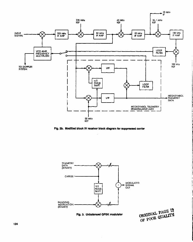
INPUTSIGNAL
325 MHzIF AMP
55 MHzIF AMP 1
0 MHz AMP
100 kHzIF AMP
10 MHz'- IF
270 MHz 45 MHz 10.1 MHzREF
REF
REF
VCO AND LOOPFREQUENCY FILTERMULTIPLIERS
100 kHzTO DOPPLER LPF I REFSYSTEM
n/2
PHASE LOOPISHIFT
FILTER
MEGASYMBOL
LPF TELEMETRYI I DATA
L MEGASYMBOL TELEMETRYDEMODULATOR ASSY
{__1
55 MHzREF
Fig. 2b. Modified block IV receiver block diagram for suppressed carrier
TELEMETRYDATA(BINARY)
CARRIER
RANGINGMODULATION(BINARY)
MODULATEDSIGNALOUT
Fig. 3. Unbalanced QPSK modulator Op^^
F^ PN QU
124

DSN Progress Report 42.44
January and February 1976
N"78-24228
Development Support — DSS 13 S-X UnattendedSystems Development
E. B. JacksonRadio Frequency and Microwave Subsystems Section
AT DSS 13 (the Venus Station), the subsystems necessary for telemetry receptionfrom spacecraft have been placed under the control of an on-station supervisorycomputer (Station Controller) and various subsystem controllers, with control inputsoriginating from Network Operations Control Center (NOCC) at JPL, and monitor inputsfrom the various Station Subsystems available to the NOCC Operator. The controlledsubsystems at DSS 13 include the Antenna and Servo, Microwave Configuration, Block111 Receiver, and Subcarrier Demodulator Assembly.
System concepts, overall system description, computer controlled subsystemcapabilities, and system testing are discussed. Testing, with control being exercised fromNOCC at JPL, has been performed on both Helios and Voyager spacecraft. The testprogram is continuing.
1. System Concepts
The goal of the DSS 13 S-X Unattended Systems Develop-ment program is to demonstrate the capability to performspacecraft tracking without the necessity for operator inputsat the station performing the tracking. Data are being collectedand will be analyzed so as to obtain a measure of the costeffectiveness of station automation, including such factors aspossible increased antenna user time availability and impact onstation MTBF which may result from the added automaticequipment. Operation of the station is exercised from a re-mote location, such as Network Operations Control Center(NOCC) at JPL, using an overall supervisory computer (StationController), controlling subsystem microprocessors for each ofthe controlled subsystems. This supervisory computer and thesubsystem microprocessors are located at the station. Control
inputs from the operator at the remote location are minimaland communications with the Station Controller are via aHigh-Speed Data Line.
For the initial capability, it was decided to constrain theautomatic capability to that required for the reception ofspacecraft downlink telemetry, including Subcarrier Demodu-lation. (The remainder of the telemetry capability at a DSNStation is already computer controlled and could be maderemote controlled with relatively minor development effort.)The subsystems chosen for modification at DSS 13 are theAntenna and Servo, Microwave Configuration, Block III Re-ceiver and the Subcarrier Demodulator Assembly (SDA). Theoutput of the DSS 13 SDA is transmitted to another DSNstation at Goldstone for processing through the Symbol
125

Synchronizer Assembly (SSA) and Telemetry ProcessorAssembly (TPA). Subsequent transmission of telemetry datato NOCC is as now done,
These subsystems at DSS 13 have now been placed undercomputer control with capabilities which permit completeoperation of these subsystems from a CRT Terminal located inNOCC, Bldg 230, at JPL. A block diagram of the systemconfiguration Is shown in figure 1. The subsystem automaticcontrol capabilities are described below.
II. System Description
A. Station ControllerThe Station Controller, the supervisory computer in this
system, is in 8080 based, JPL built, microprocessor, whichcommunicates with the controlled subsystem controllers via astandard DSN star switch. All automatically controlled Sub.systems, with the exception of the Antenna Controller, utilizea similar version of this 8080 based microprocessor. All com.munication between the NOCC Operator and the controlledsubsystems is via the Station Controller, which accepta con-figuration, predict, and operational mode selection inputs, Atthe direction of the NOCC Operator, the Station Controlleralso controls the acquisition process.
B. 26-m Antenna and ServoStarting with firm power on, but disconnec ,ed from the
Servo Subsystem, the Antenna Controller, a MODCG, tP ii/25Minicomputer, can automatically apply servo operating power,verify correct operation of the electrical and hydraulic com-ponents, and either move the antenna to any desired positionor track any desired target using operator supplied pointingangle predicts. All movements are made in High-Speed Modewith controlled acceleration, at programmed speeds, until theantenna is at its desired pointing angle. The computer thenautomatically switches to Low-Speed Mode and tracks thecomputed target path. Several environmental and servo opera•tional parameters are monitored continuously by the com-puter to ensure correct functioning. Table 1 "Servo ControlCapabilities," Table 2 "Servo Parameters Monitored," andTable 3 "Antenna Movement Modes" list the automatic moni-tor and control capabilities of this subsystem.
This automated capability may be exercised either locally,using a TermInet as the computer 1/0 device, or remotely,using the CRT Operator Terminal in NOCC. in the latter case,the input is to the Station Controller and it directs andcontrols the actions taken by the Antenna Controller,
C. Block IiI ReceiverThe Receiver Control Computer can control the receiver
local oscillator frequency and provides Initial conditions forthe receiver tracking loop filter, Acquisition of the spacecraftdownlink frequency is automatically accomplished by openinglire receiver tracking loop, sweeping the local oscillator to diccorrect frequency, detecting the presence of the downlink.activating the tracking loop, stopping the sweep and phase.locking to the downihrk carrier In a manner analogous to theactions taken manually by a skilled operator. The initial fre-quency, rate of sweep, acquisition time, start, and width of thesweep window are initially specified by the operator based onpublished predictions used by all I)SN stations. These "pre.dict" data are loaded into Cite Receiver Controller via theStation Controller.
D. Microwave ConfigurationThe configuration of the various microwave elements con•
twined in the Cassegrain fecdcone and antenna mounted elec-tronics room is controlled by the positioning of three wave-guide switches, two located in the fecdcone and one located Inthe antenna electronics roorn. The positioning of theseswitches is under the control of the Microwave ConfigurationController and is specified by configuration Information pro-vided to the Microwave Configuration Controller by the NOCCOperator, through the Station Controller. Any possible switchposition can be selected, based on configurations required bythe track to be performed, e.g., "Transmitter Dipex" or "LowNoise Listen Only" modes.
E. Subcarrier Demodulator Assembly (SDA)All of the front panel controllable, operational parameters
of the Subcarrier Demodulator Assembly, whose selection isnecessary for spacecraft subcarrier acquisition, are under thecontrol of the SDA Controller. Table 4, "Controllable SDAParameters," tabulates these parameters and their ranges. Thevalue or position of these parameters is specified by the NOCCOperator to the Station Controller, which their theSDA Controller to effect selection. At the appropriate time,the Station Controller directs the SDA Controller to effectautomatic acquisition of the spacecraft subcarrier.
III. System OperationThere are four modes through which the Unattended
Operations Control will sequence to acquire spacecraft teleme-try.
A. Station Controller InitializationWhen the Station Controller Microprocessor is first initial-
ized, it automatically enters a sequence wherein a diagnostic
126

routine checks that the Input and output ports, and litecontroller memory are fi nctionh ►g correctly. The Controllerthen prompts lite operator on input commands required toenrer the next node.
8. Controlled Subsystem InitializationIn this mode, selected by the Operator, each of the con-
trolled subsystems is initit.lized, which includes verifying thecommunications link through the Star , Switch, verifyingmeniory operability, and verifying input and output ports.Successful completion of this mode substantiates, Insofar assoftware diagnostics can determine, that the control micro•processors are functioning and are ready to accept configura•tion and predict data. The Station Controller then autonnati•sally enters the next mode.
C. Controlled Subsystem ConfigurationIn this mode, the Station Controller will accept, front tine
Operator, the configuration and predict information peculiarto the spacecraft to be tracked. This obviously Includes an•tonna pointing, receiver operating frequency, microwaveswitch positions, and SDA data rate, bandwidth, and sub-carrier frequency. Upon request, the Station Controller willdisplay to the Operator the possible choices for each con-trolled subsystem. Upon completion of the input configura-tion and predict information, lite Operator loads the varioussubsystems by instructing the Station Controller to "TRANS-FER" the entered Information. The Station Controller thenautomatically enters the next modo.
D. Controlled Subsystem OperateOnce in this mode, the Station Controller will respond to
an Operator Input command to "OPERATE," and the acquisi-tion sequence begins.
IV. Acquisition SequencingUpon receipt of the message "ON POINT" front the 26-in
Antenna Controller, the Station Controller automatically In•structs the Block III Receiver Controller to continence acquisi-tion of the spacecraft downlink carrier. Upon receipt of themessage "RECEIVER IN LOCK," the Station Controller auto•niatically instructs the SDA Controller to commence acquisi•tion of the telemetry subcarrier. When the SDA completesacquisition of the telorne:ry subcarrior, it transmits lite Ines.sage "SDA IN LOCK" to the Station Controller and theacquisition sequence Is complete, The base band spectrumoutput front the DSS 13 SDA is routed, via rite microwavelink, to another DSN station at Goldstone for symbol synchro-nization and decoding and transmission via IISDL to NOCC atbldg. 230, JPL. The NOCC Operator (DSN Controller), byobserving the Station Controller generated messages displayedon his CRT Control Terminal, can monitor subsequent porfor-tnance on his standard display, just as he would with any otherDSN station,
V. system TestingCommencing on I December 1977, the system its described
above has been tested using Helios and Voyager spacecrafttelemetry as test signals. Both DSS I I and DSS 12 have beenused as the DSN station with which telemetry processing Isaccomplished. Complete single point control, as describedherein, Its, von yet been donionstrated as the 26-ni AntennaController integration into the system is not yet completed.However, control, configuration, and predict loading of allother controlled subsystems have been repeatedly dennon-strated successfully front with no operator input tothese systems being accomplished locally at DSS 13.
Complete single point control, as described in this article, isanticipated to be demonstrated in the first week of March1978, A description of the System Software will be reportedin a later DSN Sununary.
127
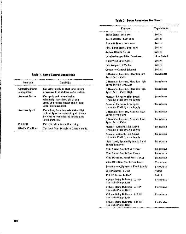
Table 2. Servo Para~* Monitored
Function Type Monitor
Table 1. Servo Control Capabilities
Function Capability
Operating Power Can either apply to start servo systemManagentmt or remove to shut down servo system,Antenna Brakes Can apply and release brakes
selectively, on either axis, or canapply and release master brake (bothaxes si ►nultancously),
Antenna Speed Can select, for either axis, either highor Low Speed as required by differencebetween antenna desired position andactual position,
PIe•iinlit Can override a prc•Ihnil warning.Disable Condition Can -m-set from Disable to Operate mode,
Brake Status, both axes SwitchSpeed selected, both axes SwitchPru»Iinhit Status, both axes SwitchFinal Limit Status, both axes SwitchSystem Disable Status SwitchLubrication Available, Gearboxes Flow SwitchRight Wrap-III) of Cables SwitchLoft Wrap-up of Cables SwitchComputer Control Selected SwitchDifferential Pressure, Elevation► Low TransducerSpeed Servo ValveDifferential P!cssurc, Elevadon High TransslucelSpeed Servo Valve, LeftDifferential Pressure, Elevation High TransducerSpeed Servo Valve, RightPressure, Elevation Iligh Speed TransducerHydraulic Fluid System SupplyPressure, Elevation Low Speed Transducerhydraulic Fluid System SupplyDifferential Pressure, Azimuth Iligh TransducerSpeed Servo ValveDifferential Pressure, Azimuth Low TransducerSpeed Servo ValvePressure, Azimuth Iligh Speed Transducerhydraulic Fluid System Supply
Pressure, Azimuth Low Speed TransducerIly6faulic Fluid System SupplyFluid Level, System Hydraulic Fluid TransducerSupply ReservoirWind Speed, South West Tower TransducerWind Speed, South East Tower TransducerWind Direction, South West Tower TransducerWind Direction, South Bast Tower TransducerTent peraItire, Hydraulie Fluid Supply Transducer75 HP Starter In-Use? Switch125 IIP Starter In-Use? SwitchVolume Being Delivered, 75 IIP TransducerIlydraulie Puntp, LeftVolume Being Delivered, 75 HP TransducerIydraulic Pump, RightVolume Being Delivered, 125 IIP TransducerHydraulic Purnp, LeftVolume Being Delivered, 125 IIP TransducerHydraulic Pump, Right
128
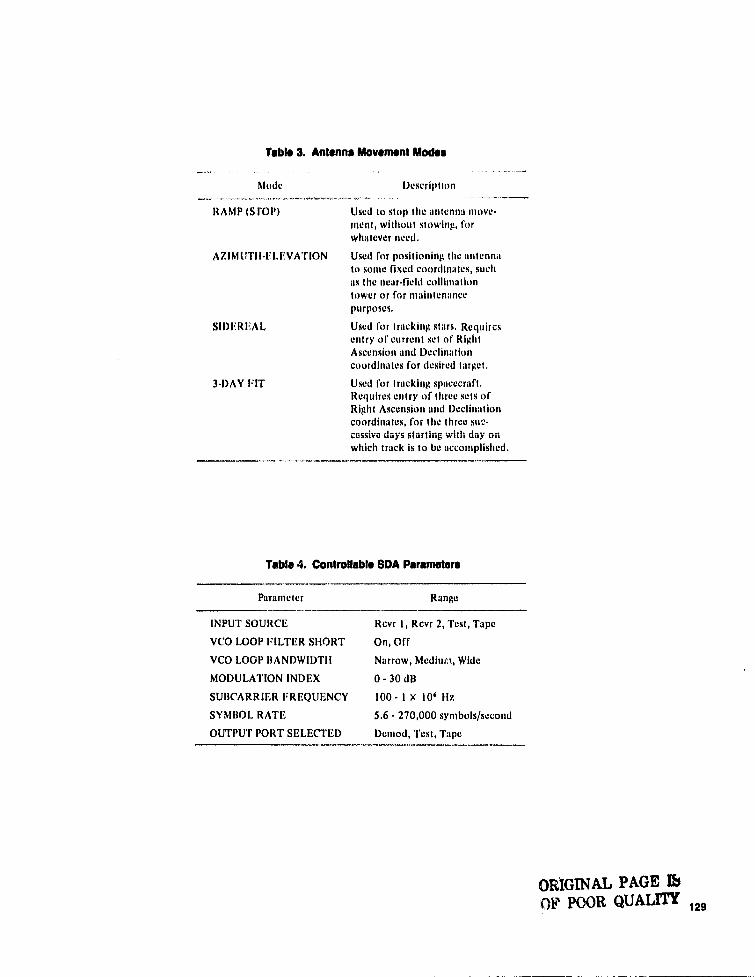
Table 3. Antenna Movement Modes
Mode
RAMP (5rOP)
A71MUT11-FLFVATION
SIDFRFAL
3-DAY FIT
Description
Used to stop file antellf a move-ment, without stowing, forwhatever need.Used for positioning the antennato some fixed coordinates, suchas file near-ficid collimationtower or for maintenancepurposes.Used for tracking stars. Requiresentry of current set of RightAscension and Declinationcoordinates for desired target,Used for tracking spacecraft.Requires entry of three sets ofRight Ascension and Declinationcoordinates, for file three suc-cessive days starting with day onwhich track is to be accomplished.
Table A. Controllable SDA Parameters
Parameter Range
INPUT SOURCEVCO LOOP FILTER SHORTVCO LOOP BANDWIDTHMODULATION INDEXSUBCARRIER FREQUENCYSYMBOL RATEOUTPUT PORT SELECTED
Rcvr 1, Rcvr 2, Test, TapeOn, OffNarrow, Medioari, Wide0-30 dB100 - I X 106 Hr.5.6 - 270,000 symbols/secondDemod, Test, Tape
ORIGINAL PAGE Ib(.)F POOR QUALITY 129
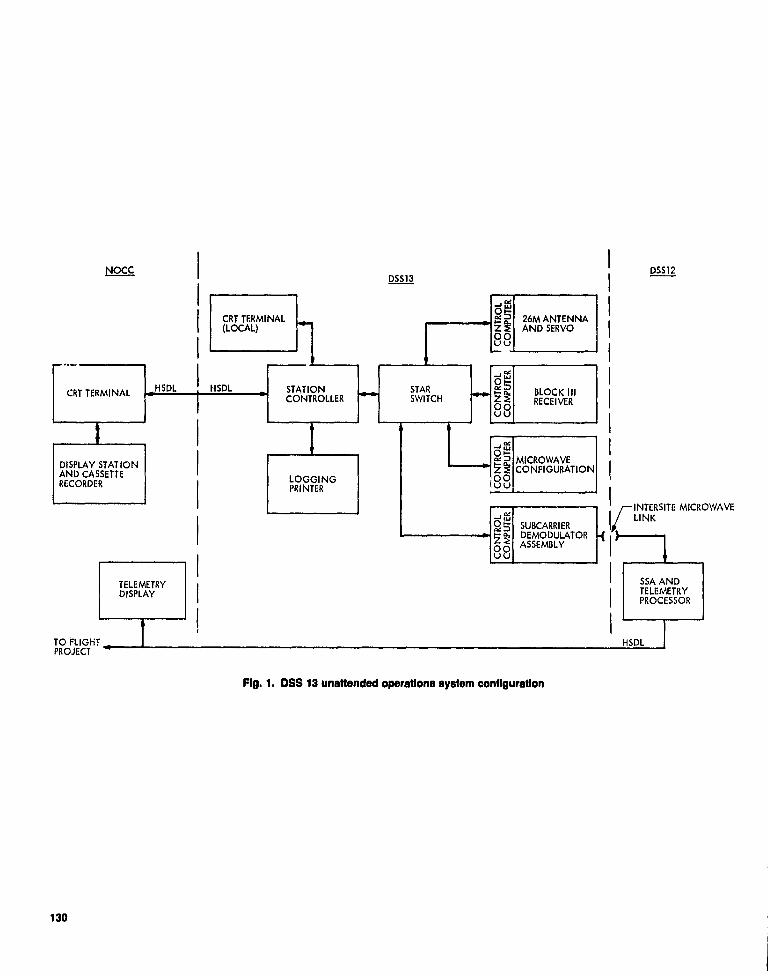
MICROWAVE
NOCC I
D5513i DSS12
rnujc%.I
Fig. I. OSS 13 unattended operations system configuration
130

DSN Progress Report 42.44
January and February 1878
N78 -24229
The DSN Standard Real-Time LanguageR. L. Schwartz, G. L. Fisher, and R. C. Tausworthe
DSN Data Systems Section
A set of requirements for tine Deep Space Network Standard Real-Time Language hasbeen recently drafted This language will be a modern high-order programming languagewell-suited to the special needs of real-time programs developed for use in the Deep SpaceStations and Network Operations and Control Center. Nearly all DSN real-time program-ming has, in the past, been done using assembly language. The implementation of astandard high-order language is being planned in order to promote tine development ofreal-time programs with higher reliability, increased programmer productivity, languagecommonality, flexibility, and re-use potential, and to provide a means for reducing thecurrent life-cycle costs of DSN software.
I. IntroductionThe DSN real-time software includes tracking and data
acquisition software and mission support software. These pro-grams, typically driven by high-speed data interrupts, haverigid input/output format requirements and must interfacewith special-purpose external hardware.
Because of the serious time constraints imposed by thehigh-speed interrupts, and the strong dependencies on externaldata formats, these programs have in the past been written, forthe most part, in assembly language. This practice has pro-duced software with a high development and maintenancecost. As the hardware base has evolved over a period of years,and as different missions have imposed their differing con-straints on the software, large existing programs have had to bealmost completely redeveloped without substantial supportfrom the earlier software.
The DSN system environment has in the past included anumber of different small- to medium-size computers, withwidely divergent characteristics. This diversified type of envi-ronment is expected to extend also into the foreseeable future.Future DSN capabilities, for example, are planned to includethe use of single-chip microprocessors as part of the standardDSN set of Control and Computation Modules (CCMs).
A standard higher-order language specifically suited to thetype of real-time programs developed by the DSN is needed topromote higher reliability, increased programmer productivity,language commonality, flexibility, and provide a means forreducing the current life-cycle cost of DSN software. A set ofrequirements for such a Deep Space Network standard real-time language has been recently drafted. This article summa-rizes that draft material. Work is continuing on refinements tothese requirements, and completion of the language specifica-tion is scheduled for the end of this fiscal year.
131

11. Brief History of Language Design forReliable Software
The development of higher-level computer programminglanguages is motivated by the desire to increase programmerproductivity and make the process of programming indepen-dent of the particular machine used. The rapidly changingcomputer hardware, together with a rapidly expanding domainof problems to be handled by means of a digital computer,necessitates the viewing of a programming language as a vehiclefor the expression of the problem in abstract terms, obviatinga detailed machine-level specification of the algorithm. Thus, aprogramming language forms an interface between its users,who are concerned primarily with the ease of expression of aproblem in abstract terms, and the instruction set on a partic-ular real machine.
As the class of problems to be solved increases in scope andcomplexity, likewise does the necessary complexity of expres-sion within the programming language. The ability of a userto understand and accurately communicate his intentionsthrough the programming language necessarily becomes moredifficult, yet at the same time becomes more crucial. Theprogramming language must accept the burden of providing avehicle for the expression of the problem in a conceptuallyclear manner in order to promote programmer understandingof what he has created.
This need has been recognized within the last decade, withvarious approaches being taken. After an early period, inwhich the development of extended assembly languages, suchas FORTRAN, (Ref. 1) paralleled the development of com-puter architecture, the need for greater abstractions from thebasic machine was recognized. The introduction of such lan-guages as ALGOL 60 (Ref. 2) and LISP (Ref. 3) signalled thebeginning of an age of higher-level languages primarily orientedtoward the user. An attempt was made to formally express thesemantics of these languages without reference to the concretemachine. This attempt at formalization of the semantics of aprogramming language was carried further by PL/1 (Ref. 4)and ALGOL 68 (Ref. 5) in very different manners. Bothlanguages sought to increase the flexibility and universality ofthe language. ALGOL 68 chose to follow a course of greaterorthogonality (using as few rules as possible, minimizing thenumber of special cases) and generalization of structure, lead-ing to almost unbounded power being given to the bewilderedprogrammer. PL/1 chose to increase the power of the languagethrough a large set of constructs and specialized rules that thebewildered programmer needed to be aware of in order toexpress his or her problem.
Soon, a realization of the high cost of software productionled to a methodology emphasizing a structured approach tothe development of computer programs. This methodology
initiated, among its supporters, a shift away from languagessuch as ALGOL 68 and PL/1, in favor of simpler languageswith features encouraging more disciplined programming.
The programming language PASCAL (Ref. 6) was the earli-est and perhaps the most successful of the languages to bedesigned at this time. PASCAL contains a minimum number offlow-of-control constructs, no default declarations or auto-matic type conversions, and a clear, concise syntax. PASCALsought to treat language semantics in a manner that wouldallow both a precise implementation specification and a de-scription of a formal (logical) system in which properties ofthe program could be derived (Ref. 7).
Various other languages, such as ALPHARD (Ref. 8),EUCLID (Ref. 9), GYPSY (Ref, 10), MADCAP-S (Ref. 11),STRUGGLE' (Ref. 12), and ALPO' (Ref. 13) have generallyfollowed the same ideas of semantic description used byPASCAL, but each has proposed somewhat different sets oflanguage features to increase program reliability, provability,power, etc.
The prolife,ation of programming languages and the result-ing program incompatibilities which have occurred in the lastfive to ten years have spurred various large users of softwaretoward the tevelopment of a standard programming language(cf. Ref. 14). The British government adopted the CORAL 66(Ref. 15) programming language as its standard in 1975, theGerman government is now completing their standardizationon the language PEARL (Ref. 16), and the French governmentis currently working on defining a French standard language.The U.S. Department of Defense has recently completed astudy to define the requirements of a DOD standard real-timehigher-order language (Refs. 17, 18), to be used in all defensesystem applications. The language, to be called DOD-1 (withPASCAL as its base language), is scheduled to be rigorouslydefined and a test translator for it implemented by early 1979.The DSN has patterned its draft requirements, summarizedhere, after the DOD requirements.
III. Goals for the DSN Standard Real-TimeLanguage
This section lists and discusses a set of general goals to yemet by the DSN standard real-time language. These are pre-sented in their approximate order of importance.
A. Life Cycle Cost EffectivQness
The overriding goal of using the DSN standard higher-orderlanguage is to reduce the life cycle cost of DSN software,
r These languages have not been implemented.
132

including initial development cost, maintenance and operationcost over the system lifetime, and costs associated with retiringa program (de-implementation), if any.
A great deal of each new DSN software system develop.ment is a repetition of programming processes that have beenwritten before. Yet, many DSN systems are started fromscratch with little benefit from this previous work, other tharwhat an individual programmer might remember (raving been apart of the previous project. Higher-order languages are pre-ferred, of course, and used when possible, but the assemblylanguage of the host machine Is usually necessary at present.Even with the "same" higher-order language, differing dialectsand local computer system alterations make it almost impos-sible to sustain a truly powerful production environment.
The DSN standard higher-order real-time language willremain stable (except under DSN Engineering Change ControlBoard direction) to ensure efficient reutilization of once-written software. Such stability will also tend to minimize tirecost of sustaining an effective production environment.
S. ReliabilityReal-time programs in the DSN control critical real-time
processes in which there is a potentially severe penalty forfaulty operation. DSN Software therefore must strive towardtotal reliability. The DSN standard real-time programminglanguage will support a programming environment which fos-ters the creation of well-structumd, readable, understandable,testable, manageable programs. Such characteristics in a pro-gram are known to promote program reliability through fewerdesign faults, decreased scope of error, and increased ease infault detection, location, and repair.
C. EfficiencyFor programs that demand it, the object code generated by
the language translator must be efficient at run-time, mainly interms of speed of execution, but also in terms of storagerequirements. The handling of high-speed telemetry interrupts,for example, necessitates rapid response and processing speeds.The DSN real-time language must therefore provide users ameans to optimize time-critical portions of their programswhen necessary. Since such optimization is likely to be verymachine-dependent, the real-time language must permit usersto access low level features of the host machine in a way notconflicting with other goals of the language.
D. MaintainabilityDSN programs written in any language must be maintain-
able. Recent industry studies (Ref. 19) and DSN qualitativestudies have shown that program maintenance accounts forsome 60% of the life-cycle costs of large programs.
Programs are made maintainable by modular construction,functional organization, localized scoping of data connections,simple control structures, tite absence of special default fea.tures, easily understandable higher-level language constructs,and a stable, controlled programming environment. Addition-ally, maintainability relates to the availability of diagnostictools and measurement aids which support the calibration,alteration, fault detection, fault isolation and location, andrepair of the program. The DSN real-time language will formthe kernel of a unified total programming system which willaccommodate all of these needs.
E. stabilityThe programming environment within which software is
developed needs to be stable in order to provide reasonableassurances of the long-term reliability, validity, maintain-ability, and reusability of DSN Software. The programmingsystem must have evolutionary potentials and avenues forchange, lest it become inadequate for future missions. How-ever, such evolution must be at a controlled, cost-effectivepace.
The DSN standard real time language and its processordesigns will be owned, implemented, and maintained by theDSN. Alterations will only be permitted as directed by DSNEngineering Change Control Board 2 action. Such changes willinvariably require assessment of impacts, costs, and benefitsprior to the implementation of new or altered features.
F. TrainingTine time required to learn the DSN standard real time
language should be relatively short. In relation to this goal, theDSN standard real time language is required to be similar Incertain ways with other languages being used in the DSN(principally MBASICtm (Refs. 20, 21)). The features of theDSN language are meant to be English-like and self-descriptive.Nevertheless, the features will be well documented, with anaccurate description of the language semantics oriented towardthe understanding level of its users.
G. TransportabilityDue to the range and diversity of programmable hardware
in the DSN, reusability of software item; relies on portabilityof program parts and trans ferabi,;ity of personnel skills amongthe various machines used. Even among real-time programswith device and machine dependencies, there are a greatnumber of operations, human and program, common amongdifferent software efforts on the different machines. Tile stan-dard language will provide a means to isolate those portions ofreal-time programs which do and do not have an inherent
2or other JPL or NASA responsible authority.
133

machine dependence, so that significant portions of programsmay be reused as needed in other DSN applications.
Briefly, the overall requirements to be satisfied by thelanguage ark':
The standard language will also increase tine transportabilityof programmer knowledge and skill. `Cite DSN standard real-time language is intended to allow each programmer to applyhis or her skills among all machines and other t ,, -Zt:s being donein ti ► e DSN.
IV.General Philosophy of RequirementsTine DSN standard read-time language is intended to be a
small, efficient, real-time-oriented, state-of-the-art, modernprogramming language for the DSN which can be adapted, viaits extensible nature, to be useful for the entire spectrum ofDSN real-time applications over the wide range of hardwarecharacteristics projected for future use. The "smallness" of thelanguage is meant to accommodate generality of expressionwhile creating efficient programs using an affordable compiler(a few man-years per implementation).
The DSN real-time operational environment differs in im-portant ways from macwtic to machine, and the needed fea-tures of DSN programs vary, depending on the particularmachine and subsystem. Because of this, those facilitiesthat can be better programmed as subsystemn-dependent orhardware-dependent subroutines or macros have not been In-cluded in the real-time language requirements. The languagetherefore will have only very basic built-in input/output facili-ties, no specific nioehanisnis for parallel processing (other thaninterlocks), no eo-routine syntax, and no built-in data types orconstructs to handle the special and diversified hardware char-acteristics found in the present DSN hardware. All of thesespecial characteristics will, however, be acconnnodatable bymacros and subroutines written in the language which, bymeans of standard libraries, can be shared by groups of users.
A general principle thai has been used in the formulation ofthe requirements is that the choice of syntax and semanticsshould follow the principle of "least astonishment." That is,there is probably a flaw in the language design if the "averageprogrammer" is astonished to learn about some aspect of thelanguage. The language is meant to appear sensible both to theaverage skilled programmer and the language specialist alike.
V. Language RequirementsThe specific requirements of the language have been asscnr
bled in keeping with the general goals and requirements philos-ophy outlined above.
(1) Statement-oriented.
(2) Supports top-down structured development ofprograms
(3) Strongly typed with full compile-time type checking
(4) Extensible, supporting data abstraction by means of adata definition facility
(S) Multi-layered language with several levels of defini-tional power
(6) Able to control non-standard external devices
(7) Allows separate compilation of program segmentswith full interface verification prior to execution
(8) Part of a total programming environment
(9) Conipilable on DSN standard minicomputers
(10) Generates code for DSN standard minicomputers andCCM's
hi this section we describe the salient features of tine languagewhich revolve around the data definition facility: its role insupporting data abstraction, its expanded definitional power,and its use in controlling real-time processes. We also brieflyintroduce the concept of a total programming environment forlanguage support. Subsequent DSN progress Report articleswill describe these and other aspects of the language in moredetail.
A. User Data Definition FacilityThe DSN standard real-time language supports data abstrac-
tion by allowing the user to define new data types and opera-tions within programs. New data types are defined by specify-ing the class of data objects comprising the type and the set ofoperations applicable to that class. The definition of the classof objects and operations oil objects is done by using thecomposition of previously defined data types and controlstructures, which, if required, call augmented by the use ofa medium-level, Moser-to-machine-language layer described insection B below.
Once defined, these abstract data types inay be used as onewould use a built-in type; one may declare identifiers rangingover the data type, then operate on the data by means of thedefined operations. By allowing access to the new object onlyby means of the pre-defined operators, an encapsulation of thedata definition supporting the abstraction occurs, therebyguaranteeing the integrity of the object being defined; that is,no unauthorized modification of the representation mayoccur.
134

The number of specialized capabilities needed for a com-mon language for all DSN real-time programming tasks is largeand diverse. fit cases, there is no consensus as to theform these capabilities should take in a programming language.No higher-order language can build in all the features u.ZfW toa broad spectrum of applications, or which would anticipatefuture applications and requirements, or even provide a univer-sally "best" capability in support of a single application area.Assembly language has had to serve as the main language toolfor most existing DSN (and other) real-time programs becauseno higher order language has been available that can accommo-date both the very low-level programming constructs as well ashigher-order abstractions.
To require that a language be implemented which has onlythose primitives in the language required to handle currentDSN applications is to build in obsolescence. Rather, the DSNreal-time language must be robust in order to survive evolvinghardware and software requirements. It must contain all thepower necessary to satisfy current applications, yet, at thesame time, contain the ability to extend that power to newand different application tasks.
A language with facilities for defining data and operationsrestricted to that data offers the capability to add newapplication-oriented structures and to use new programmingtechniques and mechanisms through descriptions written en-tirely within the language. It accommodates communicationwith non-standard external devices and diverse operating envi-ronments. The DSN standard real-time language definitionswill have the appearance and costs of features which are builtinto the language while actually being catalogued as accessibleapplication packages.
No single programming language call all the goals setforth earlier; but the DSN language, with its data and opera-tion definition facilities, can adapt to meet changing require;ments in a variety of areas while yet remaining very stableitself, thereby promoting efficiency, maintainability, reusabil-ity, etc.
S. Multi-Layered LanguageThe implementation of an abstract data type via the DSN
standard real-tine language data definition facility will bepermitted to have more expressive power than will be allowedin the rest of the user program. Inside a data definitionstructure, the pointer data type may be used in order toimplement the representation of linked structures or otherdata objects requiring the use of a pointer. Additional lower-level language features available only within the data definitionfacility include 1) a medium-level language layer which iscloser to the machine language of the host computer, 2) calls
to routines coded in other supported languages, and 3) operat-ing system calls. Each of these capabilities is particularlyimportant to support efficient control of real-time processes.
The medium-level, closer-to-the-machine-language layer willprovide a nnachine-dependent method of accommodating thoseportions of DSN real-time programs which must absolutelyhave access to specific machine architecture or bit and bytelevel manipulations. The layer will consist of the normal high-level control constructs, a set of special machine-level datatypes (such as bit and byte), and a series of built-in functionswhich provide a one-to-one correspondence to the instructionspresent oil base machine. This medium-level language layerwill thus provide machine-level access together with the high-level structuring tools present in high-level languages. A specialmachine-specific medium-level language will be required foreach implementation.
Such a median-level language concept is not new; it beganwith the medium-level language PL/360 (Ref. 22) developedby Niklaus Wirth for the IBM 360 in 1972. Since then, similarlanguages have been developed for many machines, followingthe style of PL/360.
The layered-language capability can be used, for example,to define a USN standard (but not built-in) library data typecalled, say HIGH —SPEED DATA BLOCK, with data-accessing operations coded using the medium-level layer tounpack and retrieve the information as well as allocate anddeallocate blocks as necessary.
C. Real-time Input/Output ControlThe DSN standard real-tine language will support control
of real-time processes, both through generalized input/outputoperations and the use of its data definition facilities. Thelanguage will also provide in interlock construct as a primitivemechanism for programming data definitions used for synchro-nization of parallel and concurrent processes.
A large part of many DSN real-tine programs is directlyconcerned with awkward or application-tailored input andoutput equipment, which have curious input/output instruc-tions and special status words, and which deal with data inelaborate non-standard, machine-dependent formats, none ofwhich can be clothed in the comfortable abstractions of ahigh-level programming language. As mentioned earlier, it isnot possible for a single standard higher-level real-time lan-guage to contain efficient real-tine constructs which are suffi-ciently general to be able to liandle all, or even part, of theperipheral device interfaces likely to be seen in the DSNreal-time environment.
136

Accordingly, any communication with external deviceswhich Is not possible via the built-in input/output constructsin tine DSN standard real-time language call liandled bymeans of the data definition facility. The programmer will beable to define all data type and operations whichhandle tine necessary protocols and perform all tine necessarycommunications. Inside the data definition structure, the pro-grammer will have the use of` the pointer data type, themedium-level language layer, calls to routines coded fitsupported languages, and operating system requests,
D. The Total Programming Environment
The DSN standard real-time language will not necessarilyri;quire that the object machine have an operating system, Thelanguage implementations initially will be suitable for pro-gramming both the DSN standard minicomputer and the Con-trol and Computation Modules (microprocessors), The lan-guage translator is currently planned for Implementation cmthe DSN standard minicomputer, with a crass-compilationcapability for compiling programs targeted for the Control andComputation Modules, There is no requirement for self-hosting on the CCMS.
The mere availability of .I language processor byitself is not sufficient to satisfy the goals which have been setforth earlier. The time is past in which a modern language canbe considered apart from the programming system ill itresides. The presence of synergistic tools to support programdevelopment is an essential factor in the cost-effective fabrica-tion of programs of the complexity found in DSN tasks. Forthese reasons, and following tine precedents of ECL (Ref, 23)and MBASIC"", the DSN real-tine language will require aprogramming system designed specifically for (lie language.Among the elements of this programming system are (I) anintelligent text-editor, with features designed to aid in thecoding of programs written ill language; (2) an intelligentlinkage-editor (collection program) with facilities for resolvingsnore of the module interfaces than just addresses; (3) a run-timesupport system that includes an intelligent, interactive test-
probe capability; (A) an interactive mode of program develop-ment testing, with some emulation of the real-time environment;(S) a monitor capability which will provide performancemeasurement information, such as the total number of objectcode instructions, the machine cycle times required to supporteach of the statements in the standard language, the statementexecution frequency counts, and the tine-sampling statisticscollected at run-time (either in interpretive or compiled-modeoperation). Such performance measurements lead to program-mer awareness of the time and storage characteristics of Iriscode, and call improve or optimize source code asrequired to meet applications constraints.
VI. ConclusionThe requirements reported in this article are, at this writing,
in a preliminary state, Completion of tine requirements and theendorsement of these by both programmatic and implennenta-tion organizations is required before the actual language andprocessor design activities begin. Liaison with institutiorta' andflight-support computing efforts in their current quest for aJPL-wide standard real-time language may also be expected toinfluence the final set of requirements. (The current belief isthat the DSN standard real-tinnc language call a kernelsubset of the JPL standard real-tine language, for the middle-to-large class of machines).
The authors do not mean to imply by this article that a newlanguage must be invented to fulfill the requirements suuuna-rized here. However, since no higher-order languages currentlyimplemented on DSN machines have been deenned adequatefor USN tasks (as borne out by the almost total reliance onassembly language), it seems fairly certain that. whatever lan-guage is ultimately chosen (existing, adapted, or invented), theprocessor for that language will have to be designed, docu-mented to USN standards, and implemented. Current planscall for the completion of the DSN real-linnc languag; oilMODCOMP-11 by the end of FY-80 and on the CCM's by theend of FY-81.
136

References
1. Engel, Jr„ F., et aL, "Draft Proposed ANS FORTRAN," ACM SIGPLAN Notices,
11(3), March 1976.
2. Naur, P. (ed.), "Revised Report on the Algorithmic Language ALGOL 60," Comm.
ACAI 6, pp. 1 . 17, 1963.
3. McCarthey, et al., LISP 1.5 Programmer's Manual, MIT Press, Cambridge, Mass.,1966.
4. IBM, "PL/I Language Specification," Form GY33.6003 .2, White Plaits, Now Yark.
5. van Wijogaarden, et al., "Revised Report on the Algorithmic Language ALGOL 68,"Acta btforrnatica 5, 1-3, January 1976 (also appeared in SIGPLAN Notices).
6, Wirth, N., "The Programming Language PASCAL," Acta Informatica I, Vol, 1, pp.35 .63, 1971.
7. Hoare, C.A.R., N. Wirth, "An Axiomatic Definition of the Programming LanguagePASCA.L," Aeta Informatica 2, pp. 335 .355, i973.
8, Wulf, W, A., R. L, London, M. Shaw, "Abstraction and V"rification in ALPHARD:Introduction to Language and Methodology," Computer Science Department,Carnegie Mellon University, June 1976.
9. Lampson, B. W., J. J. Horning, R. L. London, J. G. Mitchel, G. V. Popek, "Report onthe Programming; Language Euclid," ACM SIGPLAN Notices, 12(2), February 1977.
10. Ambler, A. L., et al., "Gypsy: A Language for Specification and Implementation ofVerifiable Programs," Report ICSCA-CMP-2, University of Texas at Austin, January1977.
11, Lauterback, C., C. Lucena, B. Moszkowski, "Oil Use of MADCAP for the Devel-opment of Correct Programs," Computer Science Department, Internal Mentoran-do m 132, UCLA, September 1974.
12. Berry, D. M., L. C hirica, Z. Erlich, C. Lucena, E. Walton, "STRUGGLE" StructuredGeneralized Goto-less Language," Internal Memo 147, Computer Science Depart.ntent, UCLA, 1974.
13. Dembinski, P., G. Inglas, R. Schwartz, J, Takemura, "ALPO: A Language That'sProof Oriented," in R. Uzgalis (ed.), Four Languages; Experiments in ComputerLanguage Design, UCLA-ENG-7544, Computer Science Department, UCLA, July1975,
14. American National Standards Institute Inc., reports of periodic meetings of tinecommittee in charge of Programming languages for tine Control of Industrial Pro-cesses, ISO/TC97/SC5/WG 1.
15. Official Definition of CORAL 66, Inter Establishment Committee oilApplications, ISBN 0 11 4702217, Lon6n, 1970.
16. PEARL Status as of October 1976, ANSI Committee Report ISO/TC97/SC5/WGIN21, October 1976.
17. Fisher, D. A., "A Common Programming Language for the Department of Defense,Background and Technical Requirements," institute for Defense Analysis, NTISDistribution 77 .000275, June ;976.
137

18. "Department of Defense Requirements for High Order Computer ProgrammingLanguages a- Revised Ironman," July 1977 (appearing in ACM SICPLAN Notices12(12), December 1977).
19. Ross, D., "Homilies for Bumble Standards," Comm. ACM 9(11), pp. 1 . 14, 1976,
20, MBAS1C Fundamentals, Vol. I, Jet Propulsion Laboratory Internal Document900.752, February 1974.
21, AIBASJC, Vol. Z Appendices, Jet Propulsion Laboratory, Internal Document900752, February 1974.
22. Wirth, N., "PL360-A Programming Language for the 360 Computers," Journal of theACM, Vol, IS, No. 1, pp. 37.74.
23. Wegbreit, B., et al., "The ECL Programming System," Proc. AMPS 39, pp. 253.262,1971.
138

DSN Prolym R*W 42.44
Jamiary and February 1978
On Decoding of Reed-Solomon Codes Over GF(32) andGF(64) Using the TransformTechniques of Winograd'
1. S. ReedDepartment of Electrical Engineering
University of Southern California
T. K. Truong and B. BenjauthritTDA Engineering
A new algorithm for computing a transform over GF(2"), where if = 5, 6, Is developedto encode and decode Reed-Solomon (RS) codes of length 2" - 1, Such an RS decoder Isconsiderably faster than the conventional transform decoder over GF(2").
1. Introduction
Fast real-valued transforms over the group (Z Z )" were developed first by Green (Ref. 1) to decode the (32,6) Reed-Muller code(Ref. 2) used by JPL in the Mariner and Viking space probes. Recently Gore (Ref. 3) extended Mandeibaum's methods (Ref. 4)for decoding Reed-Salomon codes. He proposed to decode RS codes with a finite field transform over GF(2"), where if is aninteger. Michelson (Ref. 5) implemented Mandelbaum's algorithm and showed that the decoder, using the transform over GF(2"),requires substantially fewer multiplications than a standard decoder (Refs. 6 .8). The disadvantage of his transform method overGF(2") is that the transform length is an odd number, so that the most efficient FFT algorithm cannot be used.
In this paper, a new algorithm based on the methods of Winograd (Refs. 9, 10) is developed to compute a transform overGF(2") for n = 5, 6. This transform algorithm over GF(2") for if = 5, 6 requires fewer multiplications than the conventional fasttransform algorithm described by Gentleman (Ref. I I). The algorithm is presented in detail in this paper only for the cases n = 5,6. This algorithm for RS codes over GF(2"), where n = 2'", has been treated previously by the authors using similar procedures(Ref. 12).
'This work was supported in part by the U.S. Air Force Office of Scientific Research under Grant AFOSR-75.279$.
139

It. Cyclic ConvolutionsThe following algorithm for the cyclic convolution of two sequences is based on Ideas due to Winagrad (Refs. 9, 10). Ut
GF(2") be the Galois Acid of 2" elements, Observe first that If X(u) n x0 + x 1 14', Y(u) n yo + y r u' for nr n I, 2, be twopolynomials over GRr), then the product T' (u) * X(u)Y(u) Is computed as follows:
T'(u) 0 X(u) Y(u) a CO " I "m + C2 Ua m
(1)
where co . x0 - yo , cr _ (xo + x ) • (yo + y t ) + x0 - yo + x r o y r , and c2 n x r • y r . Evidently there are exactly threemultiplications required to compute 11).
It is well known (Ref. 9) that if
n—tX(u) _ IE Xkuk
kn O
and
n -rY(U) = 1: ykuk
kc;A
are (n - I )-th degree polynomials, then the cyclic convolution of the coefficients of X(u) and Y(u) is given by the coefficients of
n^1T(u) = X(u) Y(u) Zkak mod (t/" ^ 1).
k=0
Now factor the polynomial V - 1 over GF(2") into irreducible relatively prime factors, i.e.,
kU" - 1 = n gl(u),
/= r
where (gl(u), g1(u)) = 1 for 10 /.
Then T(u) mod gr(u) for i = 1, 2, ... , k can be computed, using Eq. (1). To evaluate T(u) from these residues the Chineseremainder theorem is used. To show this, consider first the cyclic convolution of 3 elements. This is given in matrix form asfollows:
Y0 40 a a2 x0
y r - a t a 2 110 X (.:
Y2 a2 a0 a r x2
140

whore Yt, ap x, cGF(2") for i = Q, 1, 2. The above convolution is obtained from the coefficients of
T(u) _ (a2 +ao a+a,u2 )-(x2 +x, a+.vou~) mod (u+ 1x,12 +u+1) (3)
where (,1 + 1) and (u2 + u + 1) are the irreducible factors of it - 1 over CF(2).
To compute (3), let m(u) _ (u + 1)(u 2 + u + 1) = m,(u) m2 (U) = m,(u) M,(t1) = m2 (,1) M2(u). The system of congruencesAu) = T,(u) mod mr(u) for i = 1, 2 is given by
T,(u)'(a2 +aou+a, u2 ) • (x2 +x,u+xou 2 )mod (u- 1)=(a2 +ao +ad - (x2 + xi + xa)
and
T2 04) = (a2 +aeu +a, it 2 ) • (x2 + x,u +xo ,1 2 ) mod (u2 +14 + 1)
=_ [(a2 + a, ) + (ao + a, ) u] - [(x2 + xo ) + (x, + xo) u] mod (0 + u + 1)
By (1), T2 (u) is given by
T2 (U) (02+ad•(x2+xe)+[(a2+a1+ao+a,) '(x2+xo+x1+xo)+(a2+a,)'(x2+xo)
+(ao +a l ) • (x, +xo)] u +(ao +a,) • (x, +xo) u2
(a2 +a,) •(x 2 + xo ) + (ao + a,) • (x , + xo) + [(a2 + ad - (x2 + x i )
+(a2 + a,)(x2 +xo)] a mod (u2 + u + 1)
Evidently 3 multiplies Pre actually needed to compute T2 (u). By Chinese remainder theorem for polynomials (Ref. 13), T(u)can be reconstituted from T, (u) and T2 (u)by
T(u) = T, (u) M, (u) Ar,'(u) + T2 (u) M2 (u) M2 ' (u) mod u 3 - 1 (4)
where M,- '(u) uniquely satisfies the congruence
111,00 M^ 1 (u) = I mod m(u) for i = 1, 2.
These equations are satisfied by M i 1 (u) = 1 and M. 1 (it) = u. Hence
T(u) = (a2 + ao +a 1) • (x2 + x, + xo ) + (a2 + ad • (x2 + x,) + (a2 + a, ) • (x2 + xo ) + [(a2 + ao + a, ) • (x2 + x
i + xo )
+(a2 +a,)' (x2 +xo)+(ao+a,) • (x, +xe )] u+ [(a2 +ao +a,) • (x2 +x, +xo) + (ao +a ,)' (xi +xo)
141
ORIGINAL PAGE^
OF P00

+(a 2 +ad • (x 2 +x1)1 u2
= Yo +Y,u +Y 2 11 2 mod (u 3 - 1)
where
Yo =(a2 +ao +a,) • (x2 + x, + xo) + (a2 +a0) • (x2 +x ,)+(a2 + a,)' (x2 +xo)
Y =(a2 +QO +71)(x2 +x, tx0) + (a2 +a,) *(X2 +xo)+(ap +a I), (x , + x0 ) (5)
Y2 =(a2 +a0 t a 1 ) • (x2 +x 1 +x0) + (00 +a t ) • (x , +xo) + (a2 +ao) • (x2 +x,)
If one lets
►►10 = (a2 +ao 'ad' (x2 +x1 +x0)
►►r, = (02 + ao ) • (x2 + x, )
(6)►n 2 = (a2 +a,) • (x2 +xo)
M 3 = (ao +a,) • (x, +xo)
Then (5) becomes
YO = 710 +M I + ►112
Y, = MO + m2 + ►113
Y2 = MO + i►1 3 + ►►1,
From (6) the total number of multiplications needed to perform (2) is exactly 4. Now consider cyclic convolutions of 5elements of GF(2 11 ). Again such a convolution can be represented in matrix form as
1'o ao a l a 2 a 3 a4 X Y, a, a2 a 3 a4 ao x,
Y2 = a2 a 3 a4 a0 a, x2 (7)
Y3 a3 a4 ao a, a2 x3
Y4 a4 a0 a, a2 a 3 x4
142

where yr, a1 , x i e GF(211 ) for i = 0, 1, 2, 3, 4. Tito matrix in (7) is a S X 5 cyclic matrix. This matrix equation can be obtained alsoas the set of coefficients of
(a4 + aou + a1U2 + a2 143 + a3U4 )(x4 + x3 U + X2 U2 + X i U 3 + x0144 ) mod (u s - 1),
where 0 - 1 factors into two irreducible factors over GF(2) as follows,
u s - 1 =(u +1)(144+143+U2+U +1),
Let m(u) = (u + 1)(144 + U3 + 142 + U + 1) = m 1 (a) m 2 (U) = M1(U) M 1 (u) = m 2 (U) M2(u). The system of congruences 7(u)T,(u) mod mXu) for 1 = 1, 2 for this case is given by
T1 (U) (a4 + aou + a l U2 +a 2 U
3 +a3U4 ) • (X4 + X 3 U + X2U2 + X I U 3 + X0U4)
(a4 + '70 +a 1 +
a2 +a 3) ' (k'4 + X 3 + X2 + X 1 + x0 ) mod (u - 1) (8a)
and
72(14) =(a4 +aou+a l U2 +a2 U 3 +a 3U 4) • (X4 +x 3 14 +x2142
+ X I U 3 +X0U4)
[(a4 + a 3 ) + (ao + a 3 ) U + (a 1 + a 3 ) U2 + (a2 + a3 ) U3]
[(X4 + X0 ) + (X 3 + X0 ) 11 + (X2 + x0 ) 142
+(X I +Xo)U 3 j mod (114 +11 3 +U2 +U+ 1)
(8b)
In order to compute (8b), let Co = (a4 + a3), C 1 = (ao + a3), C2 = (a l + a 3), C3 = (a2 + a3), do = (X4 + xo), d1 = (X3 + XO),d2 = (x2 + xo), d3 = (XO + x 1 ). Thus,
T2 (u) = [C0 + C C U + C2 11 2 + C3u31 • [do + d,u + d2 U2 + d3u31 mod (U4 + U 3 + U2 + u + 1) (8c)
Now in (8c) let
Q11) = [C0 + C I U + C 2 U 2 +C 3 U 31 ' [do + d 1 u + d2 U2 + d3U3j
_ [(Co + C l u) + u2(C2 +C 3 u) [(do + d 1 U) + U2(d2 + d3U)]
ORIGINAL PAGE Ib 143
OF POOR QUALITY

Next set Ao = (co + c i u), A I = (e2 + c 3 u), Bo = (do + d i u), H l = ((12 + d3 u). Then
C(u) = (A o + u 2 A t ) - (Bo + a 2 Br)
By (1) C(u) is given by
COO = CO + CI 1t 2 + C2 u4
where
CO = A o • Bo = (co + c l u) • (do + d u)
C2 = A I • B, = (C2 + c311) • (d2 + d3u)
C, =D I - Co - C2
where D i is defined to be
D, = (A o +A i ) • (130 +L I)
= [(co + c 2 ) + (CI +
c3) uI . [(do + d2) + (d i +d 3) u)
To compute Co , C2 , D I , use (1) again to obtain,
Co = (co + c i a) • (do + d I u)
Co= •do+((co+cl)• (do + d l ) - codo -c l d i )u+c, •dlu2,
C2 = (C2 + C311) • (d2 + d3u)
C2 - d2 + ((C2 + C 3 ) • (d2 + d3) - CZ • d2 - c3 • d3) it + 03 • d3112,
and
DI = [(co + c 2 ) + (Cl + c 3 ) uI • [(do + d2 ) + (d, + d3 ) rrj
= (C0 + c2 ) • (dO + (12 ) + ((CO + C2 + C l + C 3 ) • ( do 1 [12 + d i + d 3)
- (C0 + c2)(dO + d2) - (Cl + c 3 ) (d , + d3)) u + (C I + C 3 ) • (d, + d3 ) U2
144
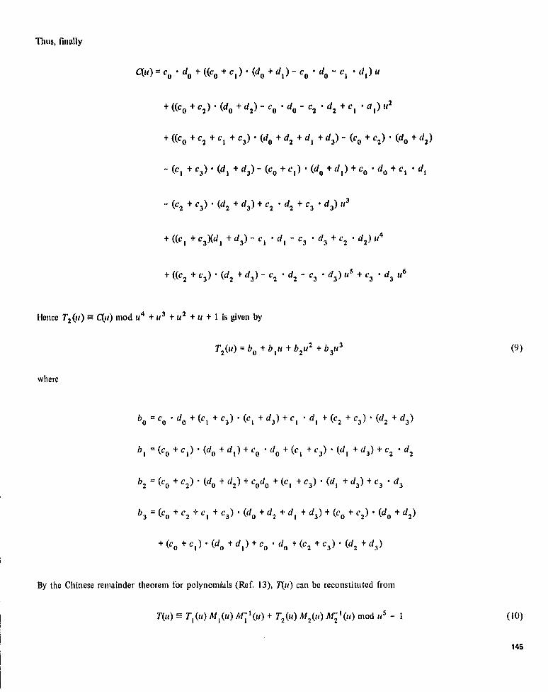
Thus, finally
Qu )=Co-do+ &0+cl)- (do + d l ) -co -do -c l - (Q u
+ ((co + c2 ) - (do + d2 ) - co - do - c2 - d2 +c, -u l ) 1t2
+ ((CD + C2 + C 1 + C 3) - (do + d2 + d l +d 3 ) - (CO + c2 ) - (do + d2)
- (Cl +C3)- (dl +d3)- (co +c l )- (do + dl) +co -do +c l -dl
- (C2 + C 3 ) - (d2 + d3 ) + C2 • d2 + C3 - d3) u3
+ ((C I + C3 )(d,+ d3) - C l - d, - C 3 - d3 + C2 - d2) it
+ ((C2 + C 3 ) - (d2 + d 3 ) - C2 - d2 - C3 - d3 ) It s + c3 - d3 116
Hence T2 (u) = C(u) mod u 4 + 14 3 + it + It 1 is given by
T2 (u) = b O + b l u + b 211 2 + b31t3
(9)
where
bo = Co - do + (Cl + C3 ) - (C l + d3 ) + C l - d l + (c2 + C3 ) - (d2 + d3)
b l = (co +c l )- (do + d l ) +co - do +(c l + C 3) - (d l +d3)+ C2 -d2
b2 = (co + C Z ) - (do + d2 ) + Ce do + (c l + C 3 ) - (d l + d3 ) + C 3 - d3
b 3 = (CO + C2 + C l + C 3 ) - (do + d2 + d l +d 3) + (C O + C Z ) - (do + d2)
+ (co + C l ) - (do + d l ) + co - do + (C-2 C 3 ) - (d2 + d3)
By the Chinese remainder theorem for polynomials (Ref. 13), Au) can be reconstituted from
T(u) = T l (u) M l (u) M l 1 (u) + T2 (u) MZ (u) M2 1 (u) mod it s - 1 (10)
145
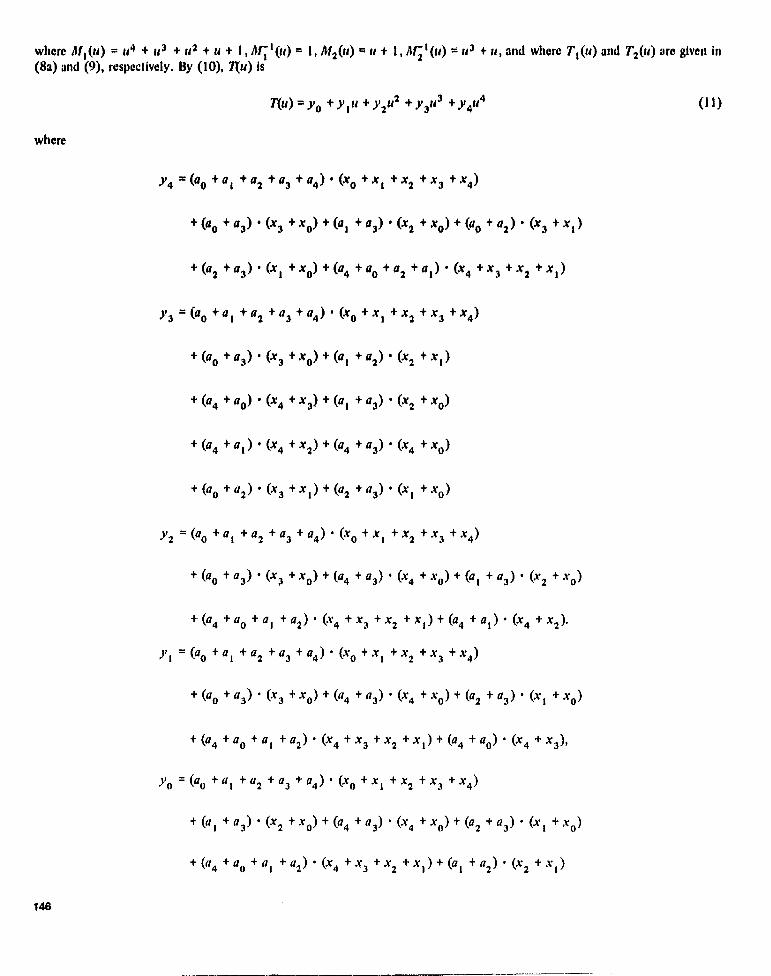
where At, (U) = 0 + 11 3 + 12 + u + I, AT I (a) = 1, Al2(11) =,I+ 1, A Z I (U) = 1 3 +u, and where T, (it) and T2 (u) are given in(8a) and (9), respectively. By (10), Au) is
7(U) =yO +y r u + Y2 U2 +y3U3 +y4U4
(11)
where
Y4 = (aO + a, + a2 + a3 + a4) - (Xp + X + X2 + X3 + x4)
+ (aO + a 3) • (X3 + XO) + (a l + a3) - (X2 + Xo) + (ao + a2) • (X 3 + X, )
+(a2+a.)-(xr + XO) +(a4+aO+a2+a,)•(x4+X3 +x2+x,)
)'3 = (aO +a, + a2 + a3 + a4 ) • (XO + X, + x2 + X 3 + X4)
+ (aO + a3 ) • (X 3 + XO) + (al + a2 ) - (X2 + X, )
+ (a4 + aO) • (X4 + X) + (a t + a3) - (X2 + XO)
+ (a4 + ad • (X 4 + X 2 ) + (a4 + a 3 ) - (X4 + XO)
+ (aO +a2 ) • (X 3 +X,) + (a2 +a3 ) - (XI + XO)
Y2 = (aO +a, + a2 + a3 + a4 ) • (XO + x, + X2 + x3 + X4)
+ (aO + a 3) • (X 3 + Xe) + (a4 +a 3) • (X4 + XO ) + (a , + a 3 ) • (X2 + XO)
+ (a4 + aO + a, +a 2) • (x4 + X 3 + X2 + X, ) + (a4 + a, ) • (X4 + X2)'
J1 1 _ (aO +a, +a 2 + a 3 + a4 ) • (XO + XI + X2 + X 3 + x4)
+ (aO +a3) • (X 3 +XO ) + (a4 +a3 ) • (X4 + XO ) + (a2 +a 3) • (XI + XO)
+(a4 +aO +a, +a2 ) • (X4 +X3 +X2 +X ,) + (a4 + ad - (X4 +X3),
yo = (ao + a, + a2 + a3 + a4 ) • (x0 + x, + x2 + X 3 + X4)
+ (a, + a3) • (X 2 + X O) + ( 74 + a 3) • (X4 + Xo) + (a2 + a 3 ) • (X r + xp)
+(a4 +aO +a, +a2) • (X4 +X3 +X2 +Xr)+(al +a2 ) • (X2 +Xr)
146

If one lets
n10 = 00 + a t + a 2 + a 3 + a4) • (x0 + x t + X2 + X 3 + x4)
m t = (ao + a 3 ) • (x3 + x0)
m2 = (a, +a 3) • (X2 + Xp)
m3 = (ao + a2 ) ' (x 3 + x t )
m4 = (a2 + a 3 ) • (X i + Xp)
(12a)
At 5 = (a4 +a0 +a2 +a t ) • (x4 +X3 +x 2 +Xd
M6 = (at +
a2 ) • (x2 +.XI)
m7 =(a4+ad'(x4+x3)
M8 = (a4 + a t ) • (x4 + x2 )
mN = (a4 + a 3 ) • (x4 + xo)
Then, (11) becomes
YO = m0 + m2 + m9 + m4 + m 5 + m6
Y, = mo + MI + m9 + m4 + m 5 + m7
Y2 =m 0 +ml +m9 +m2 +m 5 +ma (12b)
Y3 = M O + M I + m6 + m7 + m2 + M6 + m9 + m3 + Ina
V4 = nt0 +n: 1 +m 2 +m 3 +m4 +m5
Hence, by (12), the total number of multiplications required to perform (7) is 10.
Theorem 1 below, due to Winograd (Ref. 10), will be needed in the following. ORIGINAL PAGE IS
OF, POOR QUALITY 147

7heore►n 1: Let a and b be relatively prime positive integers and A be the cyclic ab X ab matrix, given by
A(x,y)= f(xty mod a-b), 0<x,y<ab.
If n is a permutation of the set of integers (0, 1, ... , ab - 1), let
B(x, y) = A (n(x), n(y))•
Then there exists a permutation n such that, if B is partitioned into b X b submatrices, each submatrix is cyclic and thesubmatrices form an a X a cyclic matrix.
In order to compute transforms of length 2" - 1 over GF(2") for n = 5 it will be necessary to compute a convolution of 15values over GF(2"). Such a cyclic convolution call be expressed in matrix form as a 15 X 15 cyclic matrix: Thepermutation n in Theorem 1 for this 15 X 15 cyclic matrix is given by
a- r0 1 2 3 4 5 6 7 8 9 10 11 12 13 1410 6 12 3 9 10 1 7 13 4 5 11 2 8 14J
With this rr the rows and columns of a 15 X 15 cyclic matrix can be partitioned into blocks of 5 X 5 cyclic matrices, suchthat each block forms a 3 X 3 cyclic matrix. This 15-point cyclic convolution in cyclic matrix form of 5 X 5 blocks is asfollows:
Eo ABC
Yo
El= B C A
Y (13)
EZC A B
Yz
where
YO
)16
Eo - y»
Y3
Y9
Y10
y,
' E 1 — }'7
Y13
)'4
Y5
yll
E _ ++ 3 32 +
Y8
Y14
148

a0 a6 a12 a3 a9
26 a12 a3 a9 ao
A a 12 a3 a9 ao a6
a 3 a9ao ab
a12
a9 ao aba12
a3
a10 a!a7 a13 a4
a l a 7a13 a4 a10
b a7 a13 a4 alo al
a13a4 alo al
a7
a4 a10 ala7 a13
a 5 all a2 a8 al 4 x0
a ll a2 ae ala as x6
^' = a 2 as ala a s al l Yo - x12
as a14 as all a2 X3
al4 a5 all a2 a8 X9
x l o x5
xi x11
Y1 = x7 Y2 = x2
X13 XS
x4xi4
149
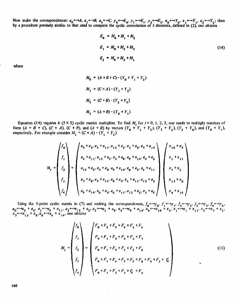
Now make the correspondences; ao *-+A, a, 4-+B, a2 +-*C' yo+--+G o, Y 1 +-►E t , y +-+E 2' x0*-► Yo, x 1 4 0 YI , xz t-► Yz ; thenby a procedure precisely similar to that used to compute the cyclic, convolution of 3 elements, defined in (2), one obtains
Eo '0 NO + MI + M2
E 3' + M2 + 11f3 (14)
E2 = Mo + M3 + MI
where
MO = (A + B + C) • (Yo + Y I +Y2)
M I = (C+A) • (Y I + Y2)
M2 = (C+B) ' (Y2 +Yo)
M3 = (A+B) • (Yo +YI)
Equation (14) requires 4 (5 X 5) cyclic matrix multiplies. To find Mf for 1 = 0, 1, 2, 3, one needs to multiply matrices ofform (A + B + C), (C + A), (C + I?), and (A + B) by vectors ( Yo + YI + Y2 ), ( Yl + Y2 ), ( Y2 + Yo ), and ( Yo + YI),respectively. For example consider MI = (C + A) - (Y I + Y2)
fo ^ ao +a s' a6 +a l 1' a 12 +a2, a3 +a 8, a9 +a 14 x 10 +xs
fl a6 +a II I a 12 +a2' a3 +a8' a9 +a 14' a 0 +a 5 'xI +x i I
Afl = f2 = a12 +a2, a3 + a8. a9 +a14' ao +a s , a6 +a l I x7 +x2
f3 a 3 +a8' a9 +a 14' ao +a s' a6 +a III a 12 +a2 x13 +x8
44 a9+a14' ao+as,a6 +a , V a 12 +a2'a3 +ae x4 4. x 14
Using the 5-point cyclic matrix in (7) and making the correspondences, fo `—'yo' fl `—'J'1' f2')'2' f3'3'3' f4`—'J'4'ao *-+ao + a5' a,+-+a6 + all' a2 +"'*a 12 +a 2' a3 *—*a3 + a8 , a4+—*a9 + a14' xo +- ►x l o + x s , x 1 4--►x 1 +.x 11 , x 2 HY7 + x2,x3 +—'+x 13 + x8,x4+---►x4 + x 14 , one obtains
fo Fo + F2 +F9 +F 4 + Fs + F6
f, FO + F, + F9 + F4 + Fs + F7
MI = J. - Fo +F I +F9 +F2 +Fs +Fs (15)
f3 Fo + F + F6 + F7 + 12 + F8 + F9 + F3 + r
J'4 Fo+F I +FZ +F3 +F +Fs
150

where
Fo 2' +aS +a6 +a l i +a 12 + a2 +a3 +aa +a9 +a14)
0 (x lo +XS +Xl +XI I +x7 +x2 +x 13 + X a +X4 +X14),
Fl .
(ao +as +a3 +aa) ' ( "l3 +Xe +X lo +XS)►
F2 " 06 +al 1 +a3 +ad • (X 7 +X2 +x lo +XS),
F3 , (ao +as +a1, +a2)' (X I +X 11 +x 13 +xa),
F4 ' (a 12 +a2 +a 3 +ae ) ' (xlo +x s +X I +x11),
Fs = (40 +a s +a6 +all +a12 +a2 +a9 +a14)
• (XI + "I I +X 7 +X2 +X 13 + x8 F X 4 +x14)
F6 = (06 +a 11 +a 12 +a2 ) • (X I +x 1 I +X7 +X2)
F7 $ (oo +as +a9 +a14) ' (X 13 +X 8 + X4 +X14)
F8 = 06 +a 11 +ag +a14) • (X 7 +x2 +X4 +x14)
F9 = 03 +ag +79 +a 14 )' (Xto +x s + x4 +X14)
Equation (15) requires 10 multiplies. In a similar manner each of the matrices MO' M2 , Ma can be obtained using 10multiplications. Thus by (14) the total number of multiplications needed to compute (13) is 40.
111. A New Algorithm for Computing a Transform over GF`2 n) of 2n —1 Points for n = 5, 6
Let GF(2") be the finite field of 2" elements. Assume that N is an integer that divides 2" - 1. Next, let the element-yeGF(2") generate the cyclic subgroup of N elements, GN = (y, y2 , ... , -y" = I ), in the multiplicative group of GF(2"). Thetransform over this subgroup GN is defined by
N-1A, = E a t-11 for G <j <N- 1
i=0ORIGINAL PAGE lbr P POOR QUALITY
where at eGF(2"). Rewrite this in matrix form as
A = W' a, (16)
161
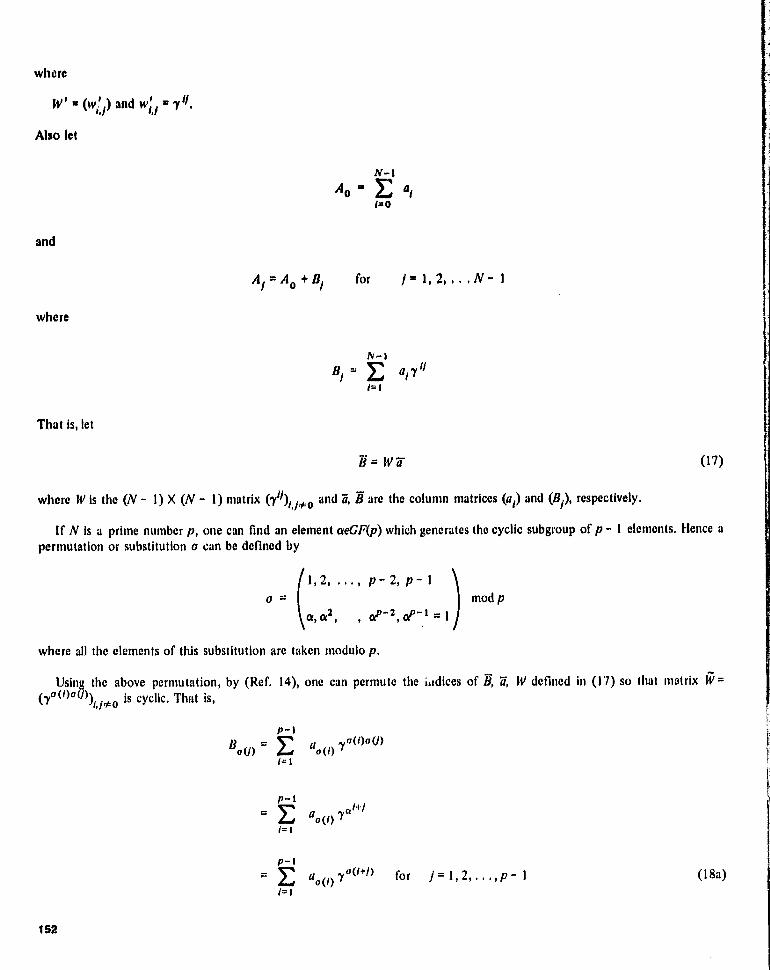
where
W, ' (W!, /) and W , : 'Y
I^"
Also let
N-1A O - F,
Im 0
and
At= AO t B, for / - 1, 2, ... N- 1
where
N-iB, aJ !1
I^ 1
That is, let
B=Wa (17)
where W is the (N - 1) X (N - 1) matrix (7')J j,,o and a, B are the column matrices (al) and (B,), respectively.
If N is a prime number p, one can find an element aeCF(p) which generates the cyclic subgroup of p - I elements. Hence apermutation or substitution o can be defined by
1, 2, ..., p- 2, p- 1Cr _ mod p
a, 012 , 01P "2, Op- t = 1
where all the elements of this substitution are taken modulo p.
Using the above permutation, by (Ref. 14), one can permute the indices of B, a, W defined in (17) so that matrix 17v=(ro(!)o(/)) is cyclic. That is,
P-1nMa(i)
BoU) ao(J)1'!- t
!=1
p-t_
a,(J)
yv(!+j) for j = 1, 2, ..., p - 1
(l8a)
!= t
152

This is reexpressed in matrix form as
9- Pa,
(18b)
where
A . (sp(i)), W " Eyo(r+r>)r,I a,
and c7 = (a,(r)).
By (182), no(/)
h a cyclic convolution of aoM
and y' (1) for J- 1, 2, • -, p I.
Let p - I - pr • pz • • • pr be the factorization of p- 1 into primes, If one lets ar - pr • pz • • p,_ t and b = p,, byTheorem I the cyclic matrix can be partitioned Into b2 - prm atrices of size a t X ar. Next let ar - all X bz, where as M pt
• • p,_z and bz = Pr- r. If az is not a prime, then a X a, cyclic matrix can be partitioned into bz matrices of size aZ X as.In general, a j = ar+t X bj+t , where b j+t is a prime. If art y 0 1, then each a ► X ar cyclic matrix can be partitioned Into b2 r
matrices of size aj+t X aj+i• Otherwise, the procedure terminates. If the number of multiplications used to compute thecyclic convolution of pj points is mr for t- 1, 2, • • •, r, then Winograd ha, shown (Ref. 10) that the number ofmultiplications needed to compute a (p - 1)-point cyclic convolution is equal to N s m I - ntz . • • ►nr.
Let N = NrN2 . , . Nk , where (Ni, Ni) = I for i O j. Using the Chinese remainder theorem for integers it is shown byWinograd in Refs, 9, 10 that the transform matrix W' defined in (16) can be transformer into the direct product of W,, Wz,... , Wk, where Wj' is the matrix of an Ni-point transform. Assume that » ► j is the number of multiplications needed toperform an Nr-point transform over GF(2") for I= 1, 2, , , . , k. Then, the number of multiplications required to compute anN-point transform is m, ►nz • .. Mk'
A. Transform over QF(25 ) of 31 PointeConsider the finite field GF(2 5 ). Since N = 2 5 - 1 = 31 is a prime p, the cyclic convolution algorithm developed in the
previous section can be used to calculate the transform of 15 points over GF(2 5 ). 1'or N = 31, the permutation a is given by
(1 2 3 4 5 6 7 8 9 10 11 12 13 14 15 16 17 18 19 20U= 3 9 27 19 26 16 17 20 29 25 13 8 24 10 30 28 22 4 12 5
21 22 23 24 25 26 27 28 29 30 ,nod 3115 14 11 2 6 18 23 7 21 l )
Let y be a 31-st root of unity in GF(2 5 ). Using the above permutation, one can pennute the indices of 13, a, W defined in
(17) so that the matrix, {V = (y°(t+J>)j * ois cyclic for I= 1, 2, ... , 30 and j = 1, 2, ... , 30. By Theorem 1, the cyclic matrixW can be first partitioned into 5 X 5 blocks as follows:
W=(A,AC,...)
153

In terms of this matrix the convolution (18b) Is given by
Tl A B C D E F S1
T2 B C A E F D S2
T3 C A B F D E S3s
T4 D E F A B C S4
Ts E F D B C A Ss
T6 F D E C A B S6
b3 b13 bls b25
b 17 b22 b23 b14
Tl b24 T2 - bl 1 T3 b27 ' T4 b7
b 12 b21 b29 b19
b6 b26 b30 bas
6 18 616y9720 7 10 y 5 7Is
69 be y20 710 7 B7 i y9
Ts = b20 T6 = b4 A = y 10 y s y l8 y9 y2
b l0 62 7s 7 1s 79 720 710
b s b 7 i 79720 y 10 y5
y8 y472 ylIt
y14 y7y19 y25 y28
y4 y271 7 16 y8 y7 y 19 y2s y2s 714
B = 72 y l 716 78y4 , C= 7 19 y2s y28 y 14 y7
7 1 y16 78 74y2 y25 y28 7 14 77 y19
y 16 ye y4 7271 y28 7 14 y7 y19 y25
where
(19)
154
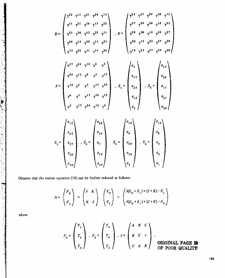
T 2 7 1 121 y26 y 13
7 11 721 y26 y 13 y22
D= 721 y26 y13 y22 7 11
726 113It
7 11 y21
713 y22 7 11 „/21 726
717 y24 7 12 76 73
724 y12 16 73 117
F= y12 Ity3 1 17 y24
y6 13 y17 72a 112
73 1 17 724 7 12 y6
a ls a28\
U23 a14
S 3 - a27 , 4 = a7
a29 a19
a30 ^a,s
123 727 1297
30 ,Y is
y27 729 y30 1 1s y23
E= y29 730 7 1sIt
727
730 yls 723 y27 129
It723 727 129 730
1
a3 a13
a ll a22
$ I = a24 , S2 = al l
a12 a21
a6 a26
a 18 a16+
a9 a8
Ss = a20 S6 = a4
a 10 a2
a s a1
Observe that the matrix equation (19) can be further reduced as follows:
F0 J K EO J(E0 +E I )+(J+K) • EI
F I K J E J(E0+EI)+Q+K)•E0
where
TI T4 A B C
F0 = T2 F2 = Ts J= B C A
ORIGINAL PAGE ICI
T3 T6 c A BOF POOR QUALM
155

t►►►d
f) !, F
A f, F f)
F f) E
Now let
1), (her ► l: ► ) • 1
112 ti (,1 i, A) • E, ('O)
(^, ; (J ,1,
K) ' FO
"hen f<<, UI .r, l' ' , f t let + /f,► , Thus, 3(15 \ 15) cyclic matrix multiplies ; ► rc licecss;► ry t ►i perl'urm ('_O), By it
proced ► t► e precisely sin ► ilar to that used to con ► putc the 15 \ 15 cyclic convolution ill tho number of multiplications
needed to compute let ill is 40. h ► a similar manner, each of the uuatrices 11 2 ; ► nd (?,► in (20) cull be ohtained with .10
multiplications. Thus, the total uumher of uulliipli.athus needed to perform ( 1 1)) is 3 \ .10 a 1.10,
B. Transform aver GF(2 6) of 63 Points
Since ;A' %; 2" 1 63 N, • iV 2 7 • Q^ by Winograd's algorithm one nerd, to compute ,tit Iransi', ilm over
GF(Y') for X,- 7 or The algonitluns 1'or con ► putinl; those Innnsliirills over GF(w") tiro ph,,cn ► tit A. let integer ifor O^i (13 lie represented by a pair (i t , i.) (i mod 3, i mad 5), Since 7 ;u ► d 1) ate relatively prin ► e, by the t'hiurse
remainder theorem,
i i t • 36 - 1, it • 28 mod 63
(2i)
is the required representation"
I.et 7 lie the 63rd root of unity ill Also let 7n 7" mod 2 and j1 77 mod 2 be the 7th and Oth roots al' unite
in (;F(? r`), respectivel), The 63rd point Ir ;IIIA,61m over ("b'(2 11 ) ill and i, is
h ,iji
q
rA rtt
L1 L '^1^ ItlI ^y
li t .i^1 , I p t i rl t
titn
rt j (^^)
156

702
712
/2
72
y42
y2
y6
772
782
y02
y2x
y42
y62
7a2
712
72
72
77
812/2 for /, = 0 9 l , 2, ... , 6
rrll U2 ) w rE a(,,,, 2 ) 72
and j2 = 0, 1, 2, ... , 82
where
or in matrix notation
(al U2 )) = Iv2' "rWhere
7Q2
702
702
y02
{V 02 y2
y02
y02
702
'Y2
u o 0 o u 0y2 y2 y2 y2 y2 72
It ly4 y 5 y6 y7 y8
2 2 2 2 2 2
6 8 I 3 5 7It y2 y2 y2 y2 y2
It y 3 y6 y0 y3
It2 2 2 2 2
3 72 6 1 572 y2 y2 y2 72 y2
72 72 72 72 72 72
7n 72 72 72 72 72
72 y2 72 72 72 72
72 7; 72 72 72 72
(l(11 0)
ay, .1)
a ( 1 1 ,2 )
a(11.3)
QtI _
a(i1.4)
a ( iI .5)
ay, (, )
a(i I .7)
ay1.8)
OEIGIN AY. pAC=^157
& YOUK ^U

Thus, (22) becomes
6Al = ly IVzar forj l = 0, 1,2,...,6
I 11=0 1
or
A 0 tV211'2
►V2 IV2 IV2 W2 IV2 a0 I
AI
IV'2 {V17 12 l
1V' y22 1 W' y32 1IV' y4
2 1{V' y52! tV' y62 1 Q ►
A2
IV'2
IV'y22 1
{V'ya2 1
IV'yG2 1
W'y 12 ►
IV' •y32 1
W'y s2 1
a2
A3
= IV'2
IV'y 32 1
IV'yG2 1
11121,y22 1
IV' y 52 1
Iv 1 7 12 1
tV'y42 1
a3
4W2' IV' ,r4
2 1{V'ry l
2 1IV' y 5
2 1IV' y22 1
W' yG2 1
IV'y3IV2' ,y3 a 4
A s {V2 1V2')'i1V2y 1
It'2y1 I 12^111
^2 y1It
^2 y1 as
AG
{V'2
IV'y62 1
W' y 52 1
IV'y42 1
N)' y32 1
IV' y22 1 IV '2 1 G
Now by (21), one obtains A o in terms of A A, as
A (o,o)
A
A (o 1)
A28
A (o 2) A 5
A (0,3)
A21
A o - A(o.M) A49
A (0,5) A 14
A (o,G) A42
A (o 7) A7
A (0,8) A35
158

Similarly
A, =
A(110)A36 A(2,0) A9
A (1.1) Ar A(2,r) A37
A(r,2)A29 A(2,2) A2
A(r.3) A57 A(2,3) A30
A,1,4) A22 72 = A(2 4) = A58
A(115)Aso A(2,5) A23
A(1,6) Al5A(2,6) A51
A (1,7) A43 A(2,7) A16
A (1,8) A8 A(2,8) A44
,
A 3 =
A(3,0)A45 A(4,0) A18
A(3,1) A10 A(4,1) A46
A(3,2)A38 A(4,2) All
A (3 3) A3 A(4,3) A39
A (; 4) = A31 A4 = A(a 4) = A4
A(3,5)A 5 A(4,5) A32
A (3,6) A24 A(4,6) A60
A(3,7)A52 A(4,7) A25
A(3,8)A17 A(4,8) A53
159

A s = I
TO
A(510) A54 A(6,0) A27
A(5'1)A19
A(6,1)Ass
A(5'2)A47
A(6,2)A20
A(5'3)A 12 A(6,3) A48
A(5,4) A40 ' W6 - A(6,4) - A13
A(5'S)As A(6,5) A41
A(5,6)A33 A(6,6) A6
A (s,7) A61 `4(6,7) A34
A (s 8) A26A(6,6) A62
a0a36 a9
a28 a1 a37
a 56 a29 a2
a21 a57 a30
a49 al _ a22 a2 = a58
a14 a50 a23
a42 (115 a51
a7 a43 al6
a35 1 a8 a44
160
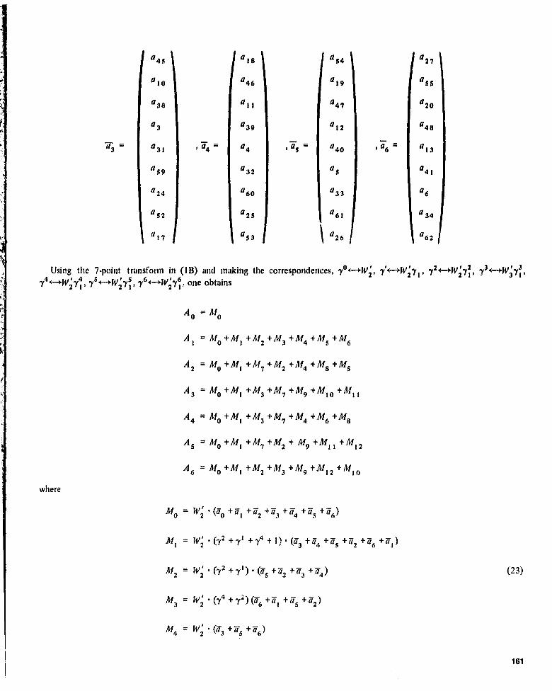
a45
a10
a36
73 a5 = ' 76
f a,4
a19
a47
a12
a40
a5
a33
061
a26
a27
a55
a20
a46
a13
a41
a6
a34
a 62 I
' 74 =
a3
a31
a59
a24
a52
a17
a1B
a46
ail
039
a4
a32
a60
a 25
a53
Using the 7-point transform ill and making the correspondences, yo4--►W21, y'_Wly" y2_—►W2y2, y3^W;yl,
y44—►WZ- ysF—► W2 y^, y6 ^— 'W2 y^, one obtains
A o = Afo
A, = All) +1112 +,113 +M4 +M 5 +M6
A 2 = MO +M 1 +11(7 +M2 +A14 +1116 +M5
A 3 = M0 +M1 +M3 +A17 +M9 +M10 +M 11
A4 = NO +M 1 +M3 +M7 +M4 +M6 +M6
A 5 = MO +M l +M7 +1112 + M9 +Af1 1 +M12
A 6 = MO +M 1 +M2 +M3 +M9 +11112 +M10
where
Mo = WZ • (17o +^- +(r2 +p3+-4+U5+Q6)
Al l = W2 • (y2 +y1+y4 + 1) • (a3 + a4 + 'IS +Q2+q6 +ll1)
M2 = 1V2 • (y2 +y l ) • (Q5 +n2 +cr3 +a4 ) (23)
M3 = WZ • (y4 +yl)(p6 +al +a5 +a2)
A14 = WZ • (a3 +Q 5 +Q6)
161

Ms = W, • (y2 + ys +yt +y6)• (us +,T,)
M6 = IVZ • (y4 +,y3 + ,y2 + ys ) • (a6 +u" S)
W2 • (y4 +y t ) • (,T6 +W1 + 3 +u4 )M7 =
Ma = Wz • (y4 +'Y' + y t + y6) • (i76 + a3 )
z (T4 +712 + ^tM9 = W )
Mto = Wz • (y4 + r3 +y2 +y s ) • (Qj +p2)
Af t = Wz•(y4 +y3 +yt+y6) •(3t +a4)
Mt 2 = Wz • (72 + yl + yt +,y6) • (°2 +Q4)
Observe that all thirteen matrix multiplies in (23) are 9-point convolutions of exactly the same form as (88). Thus onemay compute M for j = 0, 1, 2, 3, ... , 12 in (23) with a procedure similar to that used to compute the convolution definedby (813). Thus, L number of multiplications for computing M, for j = 0, 1, 2, ... , 12 is 16, excluding multiplications by y°.Hence, the total number of multiplications needed is 13 X 16 = 208.
IV. Comparison of New Algorithm with Gentleman's AlgorithmIf N = 2" - 1 = Nt - N2 .. • NA, where (N!, Nj) = I for i 96 j, Gentleman shows in References 5 and I 1 that an N-point
transform of such an N requires N(Nt +N2 + . • . + Nk - k + 1) multiplications, including multiplications by unity. Thepresent algorithm for computing the (2" - I)-point transform for n = 5, 6 and Gentleman's algorithm are compared in Table 1.The number of multiplications needed to perform these algorithms is given in both cases. Evidently for n = 5 and 6 the newalgorithm for computing the (2" - I)-point transform requires considerably fewer multiplications than Gentleman's algorithm.
V. Transform Decoder for Reed-Solomon CodesIt is shown in References 12 and 15 that RS codes can be decoded with a fast transform algorithm over Gft") and
continued fractions. There it was shown that the transform over GF(p") where p is a prime and n is an integer can be used tocompute the syndrome and error magnitudes. It follows from References 5 and 16 that the number of multiplicationsrequired to perform the syndrome and error magnitude calculations for the standard decoder is approximately (N- 1) (d- 1)+ t2 , where N is the block length of the RS code in GF(2"), d = 2t + 1 is the minimum distance of the code and t is thenumber of'allowable errors. (Note that the performance of the conventional decoder is dependent on the number of allowableerrors.)
For (31, 15) and (63, 33) RS codes, the number of multiplications needed to compute the syndrome and the errormagnitudes is given in Table 2. The new algorithm, Gentleman's algorithm, and the standard algorithm are compared inTable 2 in terms of the number of multiplications needed to compute the syndrome and the error magnitudes for decodingthese RS codes.
ORIGINAL, PAGE Ib162 OF POOR QUALITY
(23)
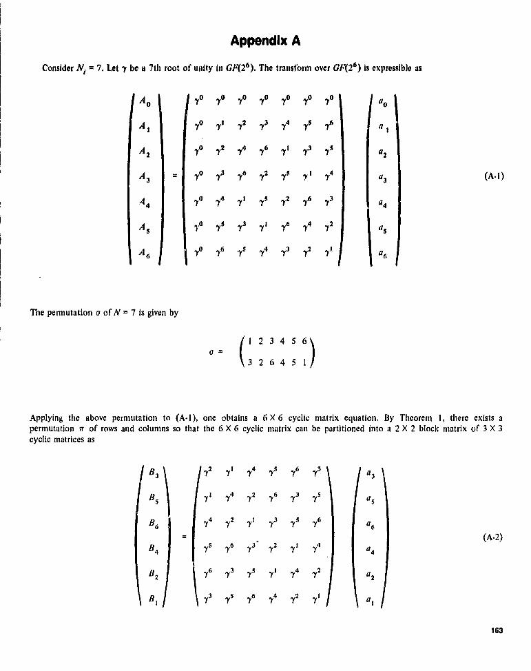
Appendix A
Consider Nr = 7. Let y be a 7(h root of unity in G!(2 6 ). The transform over G1,126 ) is expressible as
70 7o yo 70 70 7o yoa
7o yt72
y3 y4 ys76
a t
7a,y2
74,y6
lyt It 75 a2
70 It76 72
75 y' y4 a3
70 74yr 7s y2 ItIt a4
}0 7 5 y3 y' It 74,y2
as
yo y6 7174
y3y2 yA
a6
AO
IAt
Az
A3 I =
A4
As
A 6 i
(A-1)
The permutation a of N = 7 is given by
1 2 3 4 5 Gx—
3 2 6 4 5 1
Applying the above permutation to (A-1), one obtains a 6 X 6 cyclic matrix equation. By Theorem 1, there exists apermutation n of rows and columns so that the 6 X 6 cyclic matrix can be partitioned into a 2 X 2 block matrix of 3 X 3cyclic matrices as
B3 y2 ylIt
y5 y6 y3 a3
B5 yl y4 y2 y6 y3 y5 a5
B6 y4 y2 yI It y5 y6 a6
B4 y5 y6 y3 y2 ylIt
a4
B2 y6 y3 y 5 y l y4 y2a2
B, y3 y5 y6 y4 y2 y' a,
(A-2)
163

or
El A B Xt
Ez B A (X2
(XI +X2)- A+(B-A)-X2_
(XI +X2 ) - A +(B-A) - XI
D+E
D+F
where
D=(X I +X2)-A,E=(B-A)-X2,F=(B-A)-XI.
Since A and B are cyclic matrices, it is evident that the matrix B - A is also a cyclic matrix. In (A-2), D is defined as
d0 y2 It y4 Y0
D =d = y I y4 y2 Y
d2 y4 y2 y I Y2
where
Y° = a3 + a4 , Y I = as + a2 , and Y2 = a6 + a I .
Using the 3-point cyclic convolution in (2) and making the correspondences, 70 —+72, a I `^yI - a2+--*74, X0 ( OYoex f —► Y I , x2 4 ) Y2 , Y0*—+d° , Y 1 --►d 1 , y 2 '—'d2 , one obtains
('Y4 +y2+'YI) -(a3+a4 +as+a2 +a6+al.) +(y4 +y2)
d° •(a6+al+a2 +as)+(y4 +yl)•(a, +al+a3+a4)
(y4 +y2 +y I ) - (a3 +a4 +as +a2 +a, +a,) +(y4 +yl)D = d l = (A -3)
- (a6 + a I +a3 +a4 ) +(y2 +y I ) (as +a2 +a3 +a4)
(y4 +yl +y2 ) - (a3 +74 +a s +a 2 +a6 +a l ) + (12 +yl)d2
• (as +a2 +a3 +a4 ) t (y4 + y2 ) - (a, + al +as +a2)
164

Similarly,
eo y2 + f f I + y6 y4 + y3 a4
E = e 1 y1 +y6 y4 +y3 y2 +ys a2
e2 y4 +y3 y2 +ys y +y6 at
(y4 +y3 +y2 +ys + y t +y6 ) • (a4 +a2 +a I )+(,y4 +y3 +y2 +y l ) • (a I +a2 )+(y4 +y3 + y t +y6)•(a,+a4)
_ (y4+y3+V2+ ys+yt +y6).(a4+a2+a,)+(y4+y'+yt +y6).(a,+a4)+(y2+yI+yt +y6)•(a2+ad
^(y4 +y3 +y2 +ys +yt +y6 )' (a4 +a2 +a t) + (y2 +ys +yt + y6)' (a2 +a4) + (y4 +y3 +y2 +yl)' (a t + u2)
(A-4)
and
fo y2 + ys yt + y6 y4 + y3 a3
F = f, = -j + y6 y4 + y3 y2 + ys as
f2 y4 +y3 y2 +,ys yt + '16 a6
(y4 +y3 + y2 +ys i y +y6)' (a3 +a s +a6) +(y4 +y 3 +y2 +ys) • (46 +as )+(y4 + y3 +y t +y6 ) ' (a6 +a3)
(y4 +,y3 + y2 + ys + yt + y6 ) • (a3 +as +a6 ) + (y4 + y3 + j 4. • (a(, a s ) + (y4 + y 3 + y t + y6 ) ' (as +a3)
(y4 + ,y3 + y2 + ys + -1 1 + y6 ) (a 3 + a s + a6 ) + (y2 + ys + y t + y6 ) • (as + a3 ) + (y4 + y3 + y2 + ,y5) ' (a6 + as)
(A•5)
Each of the Eqs. (A•3), (A4), and (A-5) requires 4 multiplies.
Let
mp = I . (ao +a t +a2 + a3 +a4 +as +a6)
m t = (y2 +y t +y4 + I) (a3 't a4 +a, +a 2 +a6 +at)
m2 = (y2 +y t ) • (a, +a2 +a 3 +a,,)
K1 3 = (y4 + y2 ) • (a6 +a, +as +a 2) ORIvINAL PAGE Ib
OF POOR QUALMfit - 1 . (a3 +a s +a6)
165

m s . (y2 + ys + ,y I + y6 ) - (as +a3)
nlb = (y4 +y3 +y2 +ys ) - (ab +as)
M7 _ (y4 + y') • (ab +a t +a3 +a4)
mg - (y4 + ya + y' + y°) - (a, +a3)
M9 = I ' (74 +72 +a,)
►nlo - (Y4 + Y 3 +Y' + Ys ) - (al +a2)
in _ (Y4 +Y3 +y l + yb ) • (a t +a4)
M12 = (Y2 +y s +y l +ye ) • (a2 +a4)
Thus, by(A-1), (A-2), (A-3), (A4), and (A-5), one obtains
Ao = No
A I = m0 +til l +n12 +m3 + ►► 1 4 +ins +in6
A 2 = m0 t in + ►n 7 +in 2 + tit 4 +m a + tit
S
A 3 = m0 +til l + ►n 3 +m7 +m9 +nt10 + ►►111 (A-6)
A 4 = n10 +m l +nt 3 +in k +in4 +m 6 + ►n8
A s = n10 + tit l + n1 7 +in2 + ►n9 +m l 1 +n112
A6 m0 +m l +m 2 t ►n 3 +m9 +in 12 +m to
Thus, by (A-G), one observes that the number of multiplications needed to perform a 7-point transform over GF(2 7 ) is 13,including the multiplications by unit yo = 1.
Consider Nj = 3 2 . Let y be the 9th root of unity. Since 1, 2, 4, 5, 7, 8 are relatively prime to 9, the permutation v isdefined by
I, 2, 4, 5, 7, $a = (A-7)
2, 4, 8, 7, 5, 1
166

Rearranging the rows and columns of IV defined in (17) in such a manner that the elements of matrix with indices relativelyprime to 9 form a block, one has
yi i y i 2 y1 4 y i s y t 7 y1 6 y i 3 IV"' I ' at
y2 . 1 y2 . 2 y2-4 y2'5 y2 . 7 y2 . 8 y2-3 1,2-6 a 2
y4-1 y4.2 y4-4It
y4-7 y4-8 y4.3 It a4
y5 . 1 ,Y5 . 2 yP4 yS . S yS 7 y5 . 8 75-3 75.6 a 5
It y7,2 It ,Y 7.$ Y7.7 y7.8 y7,3 y7,6 a7
Y8.1 y8 , 2 78-4 y$ . $ y8-7 y8-8 y8 3 y8 6 a s
y3 . 1 y3 . 2 y3-4 y3 . 5 , 73 . 7 y3-8 73-3 y3,6a3
y6-1 y6-2 y6 .4 y6 ,5 16-7 y6 . 8 76 . 3 76 . 6 '' 06
I b1
b2
b4
b5
b7
ba
b3
I b6
(A-g)
Applying the permutation defined In (A-7) to the indices of the upper left 6 X 6 matrix of (A-n), one obtains
Y2 y4 y8 y7 y5 yi y2 a2
Y4 yK y7 y5 y 1 y2 y4 a4
Ys y7 y5 T y2 It
y8 as
Y7 y5 y 1 y2 y4 y8 y7 a7
YS y1 y2 y4 y8 y7 y5a3
Y ' y2 y4 y8 y7 y5 71a 1
By Theorem 1, the above matrix can be partitioned into a 2 X 2 block matrix of 3 X 3 cyclic blocks as
Y2. It y7 y5 y8 y2
a2
Y5 y1 y7 y4 y8 y2 y5a5
Y8 y' It y i y2 y5 y8 aA
Y7 y5 y8 y 2 y4 y1 y7 a7
Y4 y8 y2 y 5 y ' y7 y4a4
Y 1 y2 y 5 y8 y7 y4 yIal
ORIGINAL PAGE 19
nF PAR, QUALrm
(A -q)
167

Now if one makes the correspondences, y^«--►^A , fti , ryA,^+ry 7 , y a +^ y s , yr► —►y4 , ya4—+7z, B 3 4—+Yz , Ns^°► Ys,
B6 +-.+YI, Be +—+Y70 B2 *—+Y4, B t u--OY t , a3 +-+a, a s 4-- a,, a6 +-ro py, a4+--•aV 7,+-+a4, a,+^—+a I in (A•2), then by aprocedure similar to that used to compute the matrfx defined in (A'2), one obtains
Yt i Ol t +m2 + ►11 3 + 111 4 +m 5 +m6
Y4 : n1t +m 7 +1112 +1114 +"18 + 111 5
Y2 = ni t +111 3 +In d + its 9 +m 10 +mt t
Y7 = m l +t►13 +m7 +I114 +m6 +/na
YS : m t +m 7 +m2 +m9 '1'"111 + ►►112
Ya = HI +"1 2 +"1 3 +m9 +111 12 +"ito
where
nil = (y4 +yl + (a2 +a^ +as +a4 +as +al)
"1 2 = (y4 +y l )' (as +a4 +a2 +a7)
m3 = (-y' + y4 ) ' (a.+al+a5+a4)
m4 = 1 ' (a2 + as + ad
m5 = (14 +y5 + ,y l +-y8 )' (a5 +a2)
m6 = (y7 +y2 +y4 + y5) • (a8 +as)
(A• 10)M,, = (y' + y l ) • (a8 +a t +a2 +a,1)
"18 = (77 + y2 + y l + y8 ) ' (a8 +a2)
M9 = 1 ' (a7 +a4 +al)
"1 10 = (y'+y2+y4 4' y') ,(ai + a4)
►nll = (y7 +yz +yl +ye)' (al +77)
►"12 = (y`' +ys
+yl +y8)' (a4 +a7)
168

From (A-10), we know that the number of multiplications required to perform (32) is 10 excluding multiplications by yo
The last two columns of the matrix Icfir .ed in (A-8) can be obtained by computing the following 2 X 2 cyclic matrix
Xt 3 76 a3 y3 (a3 + ad + (1'3 + Y6 ) a6
(A•11)X2 76 73 a6 73 (a3 +ad +(,y3
+,y6)a3
The las, : - aws of the matrix defined in (A-8) can be obtained by computing the following cyclic matrix
Z ty3 y6 at +a4 +a7
_ (A-12)Z2 If y3 (a2 + as +a8)
y3 (at +a4 +77 +a2 +a s +as)
+(y3 +,y6) (a2 +a s +a.)
y3 (ai +a4 +a7 +a2 +a s +as)+(y3 +y6)(a t +a4 +a7)
Note that the number of ,nultiplications used to perform (A-11) or (A - 12) is 3. Thus, the algorithm for computing the 9-pointtransform is
bo = I - (ap +at +a2 +a3 +a4 +a s +a6 +a7 +a,)
b t = Y t +X t + I - ao
b 2 = Y2 +X2 +1 -ao
b3 = Z t +Z2 +I •a3+I - a 6 + I -ao
b4 '2 +X t + I • ao (A-13)
b s = Y5 +X2 +1 -ao
b6 = Z2+Zt+1 -a3 + 1 •a6 +1 -ao
b 7 = Y^ +X ^ +1 • ao ORIGIN ^vA11TY_ OF POOR
bs = Y8+X2+I -ao
From (A-13), the total number of multiplications needed to perform a 9-point transform is 16, excluding multiplications bythe ;.snit yo = 1.
169

Acknowledgement
The a.: Mors wish to thank Dr. N. A. Renzetti, Manager of Track!rrg and DataAcquisition Engineering, and the members of the Advanced Engineering Group in flanorganization at the Jet Propulsion Laboratory for their early support, suggestions, andencouragemer , , of the research which led to this paper.
References
1, R. R. Green, "Analysis of a Serial Orthogonal Decoder," Space Programs Summary37-53, Vol. 111, 1968, pp. 185.187.
2. I. S. Reed, "A Class of Multiple-Error-Correcting Codes and the DecodingScheme," IRE Trans., PGIT-4, 1954, pp. 38-49.
3. W. C. Gore, "transmitting Binary Symbols with Reed-Solomon Code," JohnsHopkins EE Report No. 73 .5, April 1973.
4. D. Mandelbaum, "On Decoding Reed-Solomon Codes," IEEE Trans. on Inform.Theory, Vol. IT-17, No. 6, pp. 707 .712, November 1971.
5. A. Michelson, "A New Decoder for the Reed-Solomon Codes Using a FastTransform Technique," Systems Engineering Technical Memorandum, No. 52,Electronic Systems Group Eastern Division GTE Sylvania, August 1975.
6. W. W. Peterson, "Error-Correcting Codes," MIT Press, Cambridge. Mass., 1961, pp.168.169.
7. S. Lin, "An Introduction to Error-Correcting Codes," Englewood Cliffs, N. J.,Prentice-Hall, 1970.
8. J. Odenwalder, et al., "Hybrid Coding Systems Study Final Report," LinkabitCorp., NASA CR 114,486, Sept. 1972.
9. S. Winograd, "On Computing the Discrete Fourier Transform," hoc. Nat. Acad.Sci. USA, 1976, 73, pp. 1005.1006.
10. S. Winograd, "On Computing the Discrete Fourier Transform," Research Report,Math. Science Dept., IBM Thomas J. Watson Research Center, Yorktown Heights,New York, 10592.
11. W. M. Gentleman, "Matrix Multiplication and Fast Fourier Transforms," BellSystem Technical Journal, 1968, pp. 1099.1103.
12. 1. S. Reed, T. K. Truong, and B. Benjauthrit, "Transform Decoding of Reed-Solomon Codes over GF(2 2 ") Using the Techniques of Winograd," Submitted toIEEE Trans. on Inform Theory.
13. E. R. Berlekamp, Algebraic Coding Theory, New York, McGraw Hall, 1968.
i4. 1. S. Reed and T. K. Truong, "Fast Mersenne Prime Transforms for DigitalFilters," to be published in the Proceedings of IEEE.
15. 1. S. Reed, R. A. Scholtz, T. K. Truong, and L. R. Welch, "The Fast Decoding ofReed-Solomon Codes Using Fermat Theoretic Transforms and Continued Frac-tions," to be published in IEEE Trans. Inform Theory.
16. G. D. Forney, "On Decoding BCH Codes," IEEE, Transactions on InformationTheory, 1T-11, October 1965.
170
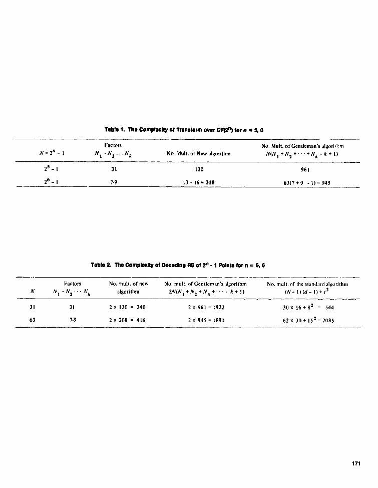
Table 1. The Complexity of Transform over QF(2n) for n = 6, e
Factors No. Mult. of Gentleman's algori+?:m
N = 2" -1 N t • N2 ... N No Ault. of New algorithm N(NI + N2 +---+N k - k + 1)
25 -1 31 120 961
26 -1 7.9 13.16=208 63(7+9 -1)=945
Table 2. The Complexity of Decoding RS of 2 n - 1 Points for n = 6, 6
Factors No. mult. of new No. mult. of Gentleman's algorithm No. must. of the standard algorithmN NI • N2 • • . N algorithm 2N(NI + N2 + N3 + • • • - k + 1) (N - 1) (d - 1) + r2
31 31 2 x 120 = 240 2 x 961 = 1922 30 x 16 + 8 2= 544
63 7.9 2 x 208 = 416 2 x 945 = 1890 62 x 30 + 15 2 = 2085
171

DSN Propreii Report 42.44
January and February 1978
N78_24231
Electron Density and Doppler RMS PhaseFluctuation In the Inner Corona
A. L. BermanTDA Engineering Office
Previous work has developed a self-consistent set of solar wind descriptors for theextended corona (S r. ¢ r < 1 AU). In this article, observations of the radial dependenceof electron density and RMS phase fluctuation are used to construct a similar andsymmetrical set of descriptors for the vastly different regime of the inner corona(r,, < r < S r.). The article concludes that the applicability of symmetrical coronaldescriptors for 5oth the inner and extended corona argues forcefully for the basic validityof the desrrip,-ion.
I. Introduction where
In a previous article (Ref. I), extensive work by J. V.Hollweg (Refs. 2 through 4) was shown to provide a frame-work in which observations of the radial dependence of phasefluctuation and electron density in the extended corona(Sr,, < r< I AU) could be combined with various assumptionsand conservation of particle flow to produce an internallyconsistent set of solar wind descriptors. These are reproducedfrom Ref. I for the extended corona as follows:
0(a) a a 1.3
N(r)ai-2.3
L t(r) at r
m = RMS phase fluctuation
Ne = electron density
Lt = transverse fluctuation scale
n = electron density fluctuation
c = ratio of electron density fluctuation to (mean) den.lity
v = radial component of the solar wind velocity
n(r) a 2.3 a = signal closest approach distance
0'P4^R QUA0V
172
nlA^ = e; e * e(r) r = radial distance
v(r) a r0.3 ro = solar radius
4 AGE I^

It should be noted that the value for 0(a) assumes a signalpath ,ntegration of about the signal closest approachpoint; au; !o the finite limits of the Earth and the spacecraft,the observed radial dependence of actual data will always besomewhat steeper than a-1.3.
The inner corona (here to be defined as ro <rF 5r.) formsa sharply distinct regime ("solar vind acceleration region")front extended corona in regard to the radial dependenceof electron density, solar wind radial velocity, etc., and henceprovides an excellent opportunity for validating the extendedcorona description. It is therefore the purpose of this article toexplore the relationship of the various coronal descriptors ofthe inner corona. Experimental observations of phase fluctua-tion and electron density in the inner corona will be shown toprovide a self-consistent set of coronal descriptors which issymmetrical with those of the extended corona. The fact thatthe same description prevails in both (vastly distinct) coronalregimes is interpreted as compelling evidence for the validityof the description.
11. Phase Fluctuation Observations In theInner Corona
The equatorial electron density model derived by Bermanand Wackley (Refs. 5 through 7) from Viking Doppler noiseand concurrent measurements of dual frequency (S minus X)range is:
2.39 X 10 81.67 X 10⁶N
6(r) = — + , electrons/cm3
r r 2.30
r = radial distance, solar radii
The doppler noise model ("ISEDC"; Ref. 5) which is the(signal path integrated) equivalent of the above electron den-sity model is:
%i)s]ISEDC, Hz =A0 Q
1 3o F(a'R)+ A t(sin a) (sin
F(a, Q) = 1 -0.05
(Q - 1T/2 + a)
3 - (a _ it/2)3
G
..0.00275 (R - rr/2 + a)5 - (a - it/2)5
( R
where
a = Sun-Earth-probe (SEP) angle, radians
0 = Earth-Sun-probe (ESP) angle, radians
A0 = 1.182 X 10⁻³
A I =4.75 X 10⁻¹⁰
For the above models, the electron density terms becomeequal valued at approximately r . 4r, while the correspondingDoppler noise terms become equal valued at approximately
r a 3rn . Doppler noise observations in the region r < 4rm arenaturally quite sparse; however 20 pass average Doppler valueshave been accumulated for this inner corona) region fromvarious Solar Conjunctions of Helios 1, Helios 2, and Viking.The method of computing "pass average" values is described indetail in Ref. 8. In deriving the ISEDC model, a three param-eter (essentially simultaneous) least squares minimisation wasperformed. The three parameters solved for were the innercorona term coefficient (A t ), and the extended corona termcoefficient (Ao) and radial index (-1.30). Figure 1 presentsthe inner corona data as compared to the inner corona term,the extended corona term, and the combined ISEDC model.The data in the region r < 4ro are clearly seen to respond tothe (integrated) inner coronal electron density term (aa-5).Figure 2 presents the correlation between the data and theISEDC model. Again the correlation is seen to be quite strong.The data in Figures I and 2 provide forceful evidence that0(a) a a- 5 in the inner corona.
111. Electron Density Observations In theInner Corona
'fhe radial dependence of electron density in the innercorona has been determined by eclipse photometry methods(van de Hulst, Ref. 9, Saito, Ref. 10, and Blackwell, Ref. 11)and via spacecraft range delays (Mulileman, Mariner G, Ref. 12,Edenhofer, Helios 2, Ref. 13), in general these experimentshave obtained consistent results which indicate a radiallydependent electron 6ensity in the inner corona of the form Ne(r) o: r 6 . Using the relationship derived by Hollweg (Ref. 2),one has for the assumption of a linear transverse scale' :
02(a) o
I r2 dr ac (a- 5) 2
a (r6 )2 -a
' The dependence with closest approach distance (a) is obtained bynoting the integral:
r
J m ra dr
1r2 -a2
is transformed via the substitution:
r = a (cos x)-tto:
In/2aa
(cos x) dx
ORIGINAL PAGE Ib
or POOR QU A TY
173

Assuming conservation of particle flow in the corona (Cuper-man and flarten, Ref. 14):
This set of coronal descriptors is compared to those for theextended corona in Table 1.
Ne(r)v(r)r2 = K
and the proportionality between electron density and electrondensity fluctuation (e = n/Ne ), ore obtains an inner corona setof self-consistent descriptors symmetrical to those for theextended corona:
O(a) a, a-s
Ne(r) a r 6
L r(r) a r
n(r) a 6
n/Ne = e; e 0 e(r)
Y(r) = r4
IV. Discussion and Conclusions
Previously, observations of the radial dependence of phasafluctuation and electron density in the extended corona wereseen to be consistent with the concept of a linear transversefluctuation scale. The fact that a vastly different regime existsin the inner :orona provides a powerful test bed to check thevalidity of the extended corona description. Observations ofdoppler noise and electron density in the inner corona, whencombined with the assumption of a linear transverse fluctua-tion scale and conservation of particle flow, are seen to beself-consistent and symmetrical with the extended corona!description. It is hereby concluded that experimental observa-tions in both the inner and extended corona provide compel-ling evidence for:
(1) The existence of a linear transverse fluctuation scale.
(2) The existence of proportionality between RMS phasefluctuation and integrated electron density.
174
References
I. Berman, A. L., "Electron Density in the Extended Corona: Two Views," bt 77reDeep Space Network Progress Report 4'-41, Jet Propulsion Laboratory, Pasadena,California, October 15, 1977.
2. Hollweg, J, V., "A Statistical Ray Analysis of the Scattering of Radio Waves by theSolar Corona," in Tire Astronomical Journal, Volume 73, Number 10, Part 1,December 1968.
3. Iloliweg, J. V., and Ilarr:ngton, J. V., "Properties of Solar Wind Turbulence Deducedby Radio Astronomical Measurements," in Tire Journal of Geophysical Research,Space Ph ysics, Volume 73, Number 23, December I, 1968.
4. HoUweg, J. V., "Angular Broadening of Radio Sources by Solar Wind 'Turbulence,"in The Journal of Geophysical Research, Space Physics, Volume 75, Number 19,July I, 1970.
5. Berman, A. L., and Wackley, J. A., "Viking S-Band Doppler RMS Phase FluctuationsUsed to Calibrate the Mean 1976 Equatorial Corona," in The Deep Space NetworkProgress Report 43-38, Jet Propulsion Laboratory, Pasadena, California, April 15,1977.
6. Berman, A. L., Wackley, J. A., Rockwell, S. T., and Kwan, M., "Viking DopplerNoise used to Determine the Radial Dependence of Electron Density in the ExtendedCorona," in The Deep Space Network Progress Report 42-38, Jet Propulsion Labora-tory, Pasadena, California, April 15, 1977.
7. Berman, A. L., "Proportionality Between Doppler Noise and Integrated Signal PathElectron Density Validated by Differenced S-X Range," in 77re Deep Space ,NetworkProgress Report 42 .38, Jet Propulsion Laboratory, Pasadena, California, April 15,1977.
8. Berman, A. L., "Phase Fluctuation Spectra — New Radio Science Information toBecome Available in the DSN Tracking System, Mark III .77," in The Deep SpaceNetwork Progress Report 42-40, Jet Propulsion Laboratory, Pasadena, California,August 15, 1977.
9, van de lfulst, If. C., "The Electron Density of the Solar Corona," Bulletin of theAstronomical Institutes of The Netherlan(Is, V011.1111e XI, Number 410, February 2,1950.
10. Saito, K., "A Non-Spherical Axisynunetric Model of The Solar K Corona of TheMinimum Type," Annals of The Tokyo Astronomical Observator y , University ofTokyo, Second Series, Volume XII, Number 2, Mitaka, Tokyo, 1970.
11. Anderson, J. D., Esposito, P. B., Martin, W. L., Thornton, C. L., and Muhleman,U.O., "Experimental Test of General Relativity Using Time Delay Data fromMariner 6 and Mariner 7," in The Astroph),sical Journal, Volume 200, August I5,1975.
12. Muhleman, D. O., Esposit y , P. B., and Anderson, J. D., "The Electron Density Profileof the Outer Corona and f ile Interplanetary Medium from Mariner 6 and Mariner 7Time Delay Measurements." 77teAstropirysicalJournal, 211, February I, 1977.
13, Ed,mhoter, P., Esposito, P. B., Hansen, R. T., Hansen, S. F., Lueneburg, E., Martin,W. L., and Zygieibaunt. A. I., "Time Delay Occultation Data of the Ilelios Space-
175

crafts and Preliminary Analysis for Probing the Solar Corona," in the Journal ofGeophysics 42, 1977.
14. Cuperman, S.. and harten, A., "Some Physical Implications of Recent Solar WindMeasurements" in Solar Wind, edited by Sonett, C. P., Coleman, P. J. Jr., and Wilcox,J. M., National Aeronautics and Space Administration, Wriadngton, D. C., 1972.
176

Table 1. Coronal desorlpilons for the Inner andextended oorons
Parameter Inner corona Extended corona(rm q6rC5rm ) (3r, IAU)
o(a) a a 5.0 a-1.3
NP (r) a r- r 2.3
Lr(r) a r r
n(r) a 6.0 r-2.3
n/NP z C. e* e(r) e; a* P (r)
1,(r) a r4.0 ro.3
ORIGINAL PAGE 11OF POOR QUALM
177

O
,
0
o
, m. .A o
2.0
2
00
1.0
COMBINED DOPPLERNOISE MODEL(ISEDC) REF. 5)
10.0
O5.0
3.19 x 10'3 J ,\(SIN 0)1.3 \\\
4.75 x 10 10 O
(SIN a) 5
D HELIOS 10 HELIOS 2O VIKING
0.1 L 1 . 1
1 2 5 10r, SOLAR RADII
Fig. 1. Doppler noise ve radial distance in the Inner corons
WJaa00
0.5
0.2
O
178
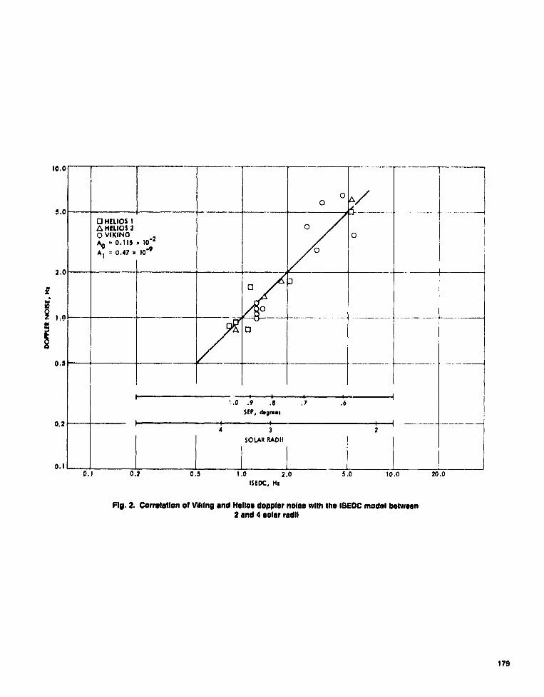
10.
O
q HELIOS iA HELIOS 2O VIKINGSA0 - 0.115 ), .9
A l -0.17x 10⁹
2.
W
oaZ 1,0
0.5
.0 .9 .8 .7SEP, degrees
0.2 h 11 3
SOLAR RADII
0.10.1 0.2 0.3 1.0 2.0
ISEDC, H:
O
Fig. 2. Correlation of Viking and Hellos doppler nolse with the 18EDC model between2 and 4 solar radii
179

08N Progreaa ROW 42.44 January and February 1878
N78®24232
The DSS Radio Science Subsystem—Rea l-TimeBandwidth Reduction and Wideband Recording of
Radio Science DataA. L. Berman
TOA Engineering Office
New radio science experiment requirements levied by the Pioneer Venus Protecthave resulted in the development of a multimission radio science subs ystem at the64-m subnet. Major functional capabilities of the DSS Radio Science Subsystem I Cj
are real-time bandwidth reduction and wideband recording of radio science das, sarticle provides a functional description of the key characteristics, requirements, andoperation of the DRS.
I. IntroductionThe Pioneer Venus Mission, with launches scheduled in
May 1978 (Pioneer Venus Orb:s^°i) and August 1978 (Pio-neer Venus Multiprobe) has two radio science experimentswith major impact c,, The Deep Space Network (DSN). InDecember 1978 the Pioneer Venus Multiprobe MissionSpacecraft will encounter the planet Venus, and at that time,the Differential Long Baseline Interferometry (DLBI) experi-ment will attempt to measure wind velocities in the at-mosphere of Venus as four probes descend through theatmosphere (Ref. 1). Also starting in December 1978, thePioneer. Venus Orbiter will undergo daily occultations byVenus for a period of approximately three months. In addi-tion, a smaller period of occultations occurs in May 1979.
As the Pioneer Venus Mission planning evolved, it becameclear that the DLBI experiment would require that the sig-nals from the four descending probes and the (spacecraft)
bus be received on one high phase stability, wideband (-2MHz) open loop receiver, and that the output of this re-ce iver be recorded on a high precision, very high rate re-corder. In addition, it was also clear that costs associatedwith processing approximately 100 S- and X-band occulta-tions of the Pioneer Venus orbiter by previously used tech-niques would be quite burdensome (Ref. 2). To reduce thesecosts, the idea was conceived of driving the open loop receiverfirst local oscillator with the predicted (atmospherically re-fracted) frequency, so that only a very narrow open loopreceiver output bandwidth would need to be recorded. Sinceprocessing costs are approximately linear wah recordedbandwidth, this procee. ure would be expected to result insubstantial savings.
As a result of these new radio science experiment require-ments, it became apparent that it would be appropriate forthe DSN to create a Radio Science System (Ref. 3). The
180

equipment at the 64-meter subnet which will perform the"real-time bandwidth reduction"' and the wideband record-ing was combined to form the DSS Radio Science Subsystem(DRS). This article describes in detail the functional operationof the DSS Radio Science Subsystem. It should be empha.sized that although the initial implementation of the DRS isgeared toward the Pioneer Venus mission, the DRS providesmultimission radio science capabilities, an.t will be exten-sively utilized in fulfillment of the radio science require•ments of other projects, such as Viking, Voyager, Galileo,etc.
11. Functional Description of the DSS RadioScience Subsystem
A. DefinitionThe DSS Radio Science Subsystem, a dedicated and integral
element of the DSN Radio Science System, performs thefollowing functions:
(1) Receives programmed oscillator (PO) frequency predic-tions and uses an error detection algorithm to verifycorrectness of predictions transmission.
(2) Reduces required open-loop receiver bandwidth viaautomatic control of a programmed oscillator whichcenters the open-loop receiver about the predicted fre-quency profile.
(3) Digitizes and formats for high-speed data line (HSDL)transmission the narrowband open-loop receiver dataand programmed oscillator data (radio science data).
(4) Digitizes and records wideband open-loop receiverdata and associated timing information (widebandradio science data) on magnetic tape.
DSS Radio Science Subsystem functions and interfaces arepresented in Fig. 1, while Fig. 2 presents functions and dataPow.
B. Key CharacteristicsThe key characteristics of the DSS Radio Science Sub-
system are listed below for functions of the Occultation DataAssembly (ODA) and the Digital Recording Assembly (DRA).
1. Real-time bandwidth reduction (ODA) key characteris-tics.
(1) Hardware and software compatibility with DSN MarkIII configuration.
'The expression "real-time bandwidth reduction" is here defined as theprocess of driving the open loop receiver local oscillator with fre-quency predictions, and subsequently filtering, digitizing, and record-ing a narrow bandwidth containing the (mixed) signal.
(2) Programmed oscillator frequency predictions receptionvia HSDL; transmission verification by an error detec-tion algorithm.
(3) Frequency predictions conversion to frequency ratesfor automatic control of programmed oscillator thatdrives S. and X-band open-loop receivers.
(4) Availability of four analog-to-digital (A-D) conversionchannels capable of being configured to digitize open-loop receiver data in the following channel vs maxi-mum sample rate combinations:
(a) One channel at 80 k samples/second
(b) Two channels at 40 k samples/second
(c) Four channels at 20 k samples/second
(d) One channel at 60 k samples/second; one channelat 20 k samples/second
(5) Availability of 8-bit quantization level of digitizedopen400p receiver data for the maximum rate; 12-bitlevel othc wise.
(6) Temporary storage of radio science data on magnetictape at the DSS for subsequent transmission to theNOCC via HSDL.
2. Wideband recording (DRA) key charam-cristics.
(1) Hardware compatability with DSN Mark 111 configura-tion.
(2) A-D conversion of wideband open-loop receiver datawith 3-bit quantization.
(3) Provision for 18-bit parallel user input interface.
(4) Provision for data recording at any discrete rate be-tween 175 k bits/second and 50 M bits/second.
(5) Provision for data recording on magnetic tape atnominal tape speeds of 19.05, 38.1, 76.2, 152.4, and304.8 cm centimeters/second.
(6) Provision for time-tagging of recorded data to onemicrosecond or better resolution.
(7) Provision for full reproduce capability (shared betweentwo transports).
(8) Provision for tape copying capability.
(9) Provision for 18-bit parallel user output interface.
(10) Eighty-minute record capability at 76.2 centimeters/second (12.5 M bits/second).
(11) Internal monitoring of recording performance.
(12) Provision for final output in analog form for monitoringpurposes.
161

C. Functional Operation1. Real-tiime bandwidth reduction. Frequency predictions
that include planetary atmospheric effects are generated bythe Network Control (NC) Support Subsystem PREDIK soft-ware program. Transmitted in the form of S-band frequenciesat the programmed oscillator (FO) level, they reach the DRSvia HSDL and are verified for correctness of transmission by anerror detection algorithm before storage for subseoiient use.
When initialized, the Occultation Data Assembly convertsthe time-tagged frequencies to frequency rate commands forthe programmed oscillator control assembly; the programmedoscillator functions to drive narrowband S- and X-band open-loop receivers. Narrowband open-loop receiver data are re-ceived by the DRS, digitized, formatted, and stored on mag-netic tape. Concurrently the programmed oscillator frequencyis counted by the DRS, formatted, and stored on magnetictape. Similarly, the ODA frequency rates to the ProgrammedOscillator Control Assembly (POCA) and POCA frequencycommands to the PO are received by the DRS, formatted, andstored on magnetic tape.
During DRS operation, manual inputs are made via the DSSMonitor & Control Subsystem (DMC), and, similarly, the DRSis monitored from the DMC.
The digitized open-loop receiver data and the various pro-grammed oscillator frequency data are transmitted from theDSS to the NOCC via HSDL in nonreal time or via tapeshipment. Users gain access to the radio science data viaIntermediate Data Records (IDR) written by the Ground Com-munications Facility (G%--F) Data Records Subsystem. Figure 3presents a functional block diagram of the Occultation DataAssembly.
2. Wideband recording. Wideband open-loop receiver datafrom the Multimission Open-Loop Receiver (MMR), whichmay contain multiple probe signals and receiver calibrationtones, are received by the Digital Recording Assembly. Thesedata are digitized at a quantization level of 3 bits and arerecorded on 18 tracks of magnetic tape at a nominal tapespeed of 76.2 centimeters/second (12 M bits/second). Concur-rently, timing information' received from the Frequency andTiming Subsystem (FTS) is recorded on two additional tracks.During recording, performance is monitored internally withinthe DRA.
The DRA simultaneously records on two separate trans-ports. Subsequent to these recordings, duplicate copies may beproduced on the DRA. The recorded wideband tapes aresubsequently shipped to the Compatibility Test Area (CTA21) Radio Science Subsystem via Network Information Con-trol (NIC).
111. Functional Requirements of the DSSRadio Science Subsystem
A. Functional Requirements for Real-TimeBandwidth Reduction
1. Programmed oscillator frequency predictions. The ODAshall accept via HSDL and store programmed oscillator fre-quency predictions in the form of time tagged S-band frequen-cies at the programmed oscillator level (-46 MHz).
2. Prediction error detection. The ODA shall include anerror detection algorithm in conjunction with the NC SupportSubsystem PREDIK softw=are program. This shall be for thepurpose of verifying prediction consistency from generationthrough the ODA.
3. Programmed oscillator frequency control. The ODAshall convert time-tagged frequency predicticn q to frequencyrates, and provide the results to the Programmed Oscilla!o,Control Assembly (POCA) for programmed oscillator controlof narrowband S- and X-band open-loop receivers.
4. Signal presence and ODA operation verification. TheODA shall provide a reconstructed analog receiver signal to theSpectral Signal Indicator for real-time verification of signalpresence in the receiver bandwidth and verification of ODAoperation.
S. Occultation data processing and storage. The ODA shallreceive, digitize, and store time-tagged narrowband S- andX-band open-luop receiver output. The following are missionperiod requirements:
(1) Pioneer Venus Orbiter
Channels: 1 S-band, 1 X-bandBandwidths: I kHz S-band, 3 I.Hz X-band
5 kHz S-band, 15 kHz X-bandQuantization: 8-bit
(2) Pioneer Venus Orbiter (solar corona)
Channels: 1 S-band, 1 X-bandBandwidths: 1000 Hz S- and X-band
500 Hz S- and X-band1 36 Nz S- and X-band
Quantization: 8-bit
(3) Voyager (first Jupiter encounter)
Channels: 1 S-band, I X-bandBandwidths: 2.5 kHz S-band, 7.5 kHz X-band
10 kHz S-band, 301 kHz X-handQuantization: 8-bit
182
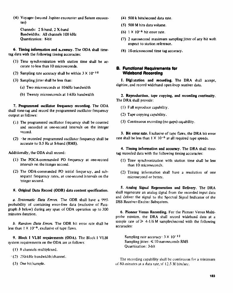
(4) Voyager (second Jupiter encounter and Saturn encoun.ter)
Channels: 2 S-band, 2 X-bandBandwidths: All channels 100 kHzQuantization: 8-bit
6. Timing information and accuracy. The ODA shall time.tag data with the following timing accuracies:
(1) Time synchronization with station time shall be ac-curate to less than 10 microseconds.
(2) Sampling rate accuracy shall be within 3 X 10- 10
(3) Sampling jitter shall be less than:
(a)Two microseconds at 10-kHz bandwidth
(b) Twenty microseconds at 1-kHz bandwidth
7. Programmed oscillator frequency recording. The ODAshall time-tag and record the programmed oscillator frequencyoutput as follows:
(i) The programmed oscillator frequency shall be countedand recorded at one-second intervals on the integer-econd.
(2) , he recorded programmed oscillator frequency shall beaccurate to 0.5 Hz at S-band (RMS).
Additionally, the ODA shall record:
(1) The POCA-commanded PO frequency at one-secondintervals on the integer second.
(2) The ODA-commanded PO initial frequency, and sub-sequent frequency rates, at one-second intervals on theinteger second.
8. Original Data Record (ODR) data content specification.
a. Svstematic Data Errors. The ODR shall have a 99%probability of containing error-free data (exclusive of Para-graph b below) during any span of ODA operation up to 300minutes duration.
b. Random Data Errors. The ODR bit error rate shall beless than I X 10- 6 , exclusive of tape flaws.
9. Block I VLBI requirements (ODA). The Block I VLBIsystem requirements on the ODA are as follows:
( I ) 8 channels multiplexed., (2) 250-kHz bandwidth/channel.
(3) One bit/sample.
(4) 500 k bits/second data rate.(5) 500 M bits data volume.
(6) 1 X 10-6 bit error rate.
(7) 2 nanosecond maximum sampling jitter of any bit withrespect to station reference.
(8) 10-microsecond time tag accuracy.
B. Functional Requirements forWideband Recording
1. Digitization and recording. The DRA shall accept,digitize, and record wideband open-loop receiver data.
2. Reproduction, tape copying, and recording continuity.The DRA shall provide:
(I) Full reproduce capability.
(2) Tape copying capability.
(3) Continuous recording (no gaps) capability.
3. Bit error rate. Exclusive of tape flaws, the DRA bit errorrate shall be less than I X 10- 6 at all required tape speeds.
4. Timing information and accuracy. The DRA shall time-tag recorded data with the following timing accuracies:
(1) Time synchronization with station time shall be lessthan 10 microseconds.
(2) Timing information shall have a resolution of onemicrosecond or better.
5. Analog Signal Regeneration and Delivery. The DRAshall regenerate an analog signal from the recorded input dataand deliver the signal to the Spectral Signal Indicator of theDSS Receiver-Exciter Subsystem.
6. Pioneer Venus Recording. For the Pioneer Venus Multi-probe mission, the DRA shall record wideband data at asample rate of> 4 . 1/6 M samples/second with the followingaccuracies:
Sampling rate accuracy: 3 X 10' 12
Sampling jitter: E 10 nanoseconds RMSQuantization: 3-bit
The recording capability shall be continuous for a minimurno1 80 minutes at a data rate,.)f 12.5 M bits/sec.
183

7. Block If VLBI Requirements (DRA). Block II VLBIsystem requirements on the DRA are as follows:
(1) 8 channels.
(2) 2-MHz bandwidth/channel.
(3) 1 bit/sample.
(4) 32 M bits/second data rate.
(5) 10 11 bits data volume.
(6) 1 X 10-6 bit error rate.
(7) 2 nanosecond maximum sampling jitter of any bit withrespect to station reference.
(8) 5-microsecond time tag accuracy.
IV. DRS Planned Implementation ScheduleThe planned implementation dates for the various DRS
capabilities are presented below:
Digital Recording Assembly
DSS 14 . . . . . . . . . . . . . . . . . Feb. I5, 1978DSS 43 . . . . . . . . . . . . . . . . . Feb. 15, IY78DSS 63 .. . . .. .. ... . . . .. . Feb. 15, 1979
DSS Radio Science Subsystem
DSS 14 . . . . . . . . . . . . . . . . . . July 1, 1978DSS 43 .. . . . . .. . .. . . .. . . . July 1, 1978DSS 63 (ODA only) .. .. . .. .. . . Dec. 1, 1978
Programmed Osciliatoi Monitor
DSS 14 .. . . . . . ... . . ... . . . Oct. 1, 1978DSS 43 . . . . . . . . . . . . . . . . . . Oct. 1, 1978DSS 63 . . . . . . . . . . . . . . . . . . Dec. 1, 1978
Very Narrow Bandwidth Capability
DSS 63 . . . . . . . . . . . . . . . . . . Dec. 1, 1978DSS 14 . . .. . . .. . .. . .. . . . April 1, 1979DSS 43 . . .. . . . . . . . . . . . . . A pril 1, 1979
Four-channel Capability (Saturn Ring Experiment)
DSS 14 . . . . . . . . . . . . . . . . . April 1, 1979DSS 43 .. . .. . . . ... . . .. . . April 1, 1979DSS 63 . . . . . . . . . . . . . . . . . April 1, 1979
Spectral Signal Indicator Display Processing
DSS 14 . . . . . . . . . . . . . . . . . . July 1, 1979DSS 43 . . . . . . . . . . . . . . . . . . July I, 1979DSS 63 . . . . . . . . . . . . . . . . . . July 1, i979
DMC Interface
DSS 14 . . . . . . . . . . . . . . . . . . July I, 1979DSS 43 . . . . . . . . . . . . . . . . . . July 1, 1979DSS 63 . . . . . . . . . . . . . . . . . . July 1, 1979
Wideband Interface
DSS 14 . . . . . . . . . . . .. . . . . . July 1, 1979DSS 43 . . . . . . . . . . . . . . . . . . July 1, 1979DSS 63 . . . . . . . . . . . . . . . . . . July 1, 1979
References
I. Berman, A. L., and Molinder, J. I., "The CTA 21 Radio Science Subsystem —Non-Real-Time Bandwidth Reduction of Wideband Radio Science Data," in The DeepSpace Network Progress Report 42-41, Jet Propulsion Laboratory, Pasadena, Cali-fornia, October 15, 1977.
2. Berman, A. L., "Planetary Atmosphere Modeling and Predictions" in Tire Deep SpaceNetwork Progress Report 42-42, Jet Propulsion Laboratory, Pasadena, California,December 15, 1977.
3. Mulhall, B. D. L., "DSN Radio Science System Description and Requirements" in TheDeep Space Network Progress Report 42-39, Jet Propulsion Laboratory, Pasadena,California, June 15, 1977.
tea 01 114 At PAGE IS
OF

DSS SUBSYSTEM DSN-JPL SUBSYSTEMINTERFACES INTERFACES
FUNCTIONS
• RECEIVES PROGRAMMED OSCILLATOR FREQUENCY PREDICTIONSCONFIGURATION
DSS MONITOR AND CONTROL • USES ERROR DETECTION ALGORITHM TO CHECK PREDICTION& CONTROL CONSISTANCY FROM NC SUPPORT SUBSYS i EM TO DSSSUBSYSTEM SUBSYSTEM STATUS RADIO SCIENCE SUBSYSTEM
AND ALARMS
• CONVERTS PROGRAMMED OSCILLATOR FREQUENCYPREDICTIONS TO FREQUENCY RATES FOR CONTROL OF
DSSPROGRAMMED OSCILLATOR
RECEIVER-NARROWBAND OPEN-LOOP RADIO GCF DATA
EXCITERRECEIVER DATA, PROGRAM- • DIGITIZES NARROWBAND OPEN-LOOP RECEIVER DATA AND SCIENCE RECORDSMED OSCILLATOR DATA STORES ON MAGNETIC TAPE DATA SUBSYSTEMSUBSYSTEM
• FORMATS AND TRANSMITS DIGITIZED TIME-TAGGEDNARROWBAND OPEN-LOOP RECEIVER DATA AND PROGRAMMED
DSS OSCILLATOR DATA ( RADIO SCIENCE DATA) VIA HSD INRECEIVER- ANALOG SIGNAL TO NONREAL TIMEEXCITER SPECTRAL SIGNAL
SUBSYSTEM INDICATOR• DIGITIZES AND RECORDS WIDEBAND OPEN-LOOP RECEIVER
DATA AND ASSOCIATED TIMING INFORMATION (WIDEBANDRADIO SCIENCE DATA) ON MAGNETIC TAPE
DSSRECEIVER- PROGRAMMED OSCILLATOR• PROVIDES CONFIGURATION AND STATUS DATA
PROGRAMMED OSCILLATOR KEXCITER FREQUENCY CONTROL FREQUENCY PREDICTIONS SUPPORT
SUBSYSTEM• PROVIDES ANALOG SIGNAL TO SPECTRAL S!;NAL INDICATOR SUBSYSTEM
TO VERIFY SIGNAL PRESENCE IN THE ORS RECORDED DATA
DSS CTA 21 RADIORECEIVER- WIDEBAND OPEN-LOOP WIDEBA!W) RADIO SCIENCESCIENCEEXCITER RECEIVER DATA DATA VIA NIC •
SUBSYSTEM SUBSYSTEM
ucc FREQUENCY& TIMING TIMING INFORMATION
*NETWORK INFORMATION CONTROLSUBSYSTEM
Rg. 1. DSS RI) db Sdom Subsystmn fundk ns and
coN
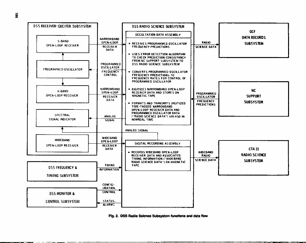
mCD
DSS RECEIVER- EXCITER SUBSYSTEM DSS RADIO SCIENCE SUBSYSTEMGCF
OCCULTATION DATA ASSEMBLYDATA RECORDS
• RECEIVES PROGRAMMED OSCILLATORS-BAND
NARROWBANDOPEN-LOOP RADIO SUBSYSTEMRECEIVEROPEN-LOOP RECEIVER FREQUENCY PREDICTIONS SCIENCE DATADATA
• USES ERROR DETECTION ALGORITHMTO CHECK PREDICTION CONSISTANCYFROM NC SUPPORT SUBSYSTEM TO
PROGRAMMED DSS RADIO SCIENCE SUBSYSTEMOSCILLATORPROGRAMMED OSCILLATORFREQUENCY • CONVERTS PROGRAMMED OSCILLATORCONTROL FREQUENCY PREDICTIONS TO
FREQUENCY RATES FOR CONTROL OFPROGRAMMED OSCILLATOR
NARROWBAND • DIGITIZES NARROWBAND OPEN-LOOP NCX-BAND OPEN-LOOP RECEIVER DATA AND STC41ES ON PROGRAMMEDRECEIVEROPEN-LOOP RECEIVER MAGNETIC TAPE OSCILLATOR SUPPORTDATA
• FORMATS AND TRANSMITS DIGITIZED FREQUENCY SUBSYSTEMPREDICTIONSTIME-TAGGED NARROWBANDOPEN-LOOP RECEIVER DATA ANDPROGRAMMED OSCILLATOR DATA
SPECTRAL ANALOG ("RADIO SCIENCE DATA"1 VIA HSD INSIGNAL INDICATOR NONREAL TIMESIGNAL
ANALOG SIGNAL
WIDE BANDWIDE BAND OPEN-LOOP DIGITAL RECORDING ASSEMBLYOPEN-LOOP RECEIVER RECEIVERDATA CTA 21
• RECORDS WIDEBAND OPEN-LOOP WDEBANDRECEIVER DATA AND ASSOCIATED RADIO RADIO SCIENCETIMING INFORMATION(" WDEBAND SCIENCE DATA SUBSYSTEMRADIO SCIENCE DATA ") ON MAGNETIC
TIMING TAPEDSS FREQUENCY & INFORMATION
TIMING SUBSYSTEM
CONFIG-URATION,
DSS MONITOR &CONTROL
CONTROL SUBSYSTEM STATUS,ALARM
F19- 2 DW Radio S &ftystem ftffwUons aW cl^ft tt w

PROGRAMMED
OSCILLATOR
OCCULTATION
CONVERTER
SUBASSEMBLY I TER110MINET I
X-BAND
OPEN-LOOP
RECEIVER
AID
CONVERTER
MODCOMP
11125
COMPUTER DISK
DIA
CONVERTER
^d
"d
49'3C^3 COUNTER
NC SUPPORTHSDL SUBSYSTEM
PREDIK
HSDLGCF DATA
RECORDS
SUBSYSTEM
SPECTRAL
SIGNAL
INDICATOR
PROGRAMMEDOSCILLATORCONTROL
ASSEMBLY
OCCULTATION DATA ASSEMBLY
AID GCF
CONVERTER --- --- DATA RECORDSSUBSYSTEM
COMP TAPE
RECEIVER -EXCITER
SUBSYSTEM
S-BAND
OPEN-LOOP
RECEIVER
* SHIPPED Vu NH;
Fig. & Occuttetlon Dale Amy fundWW bbr&
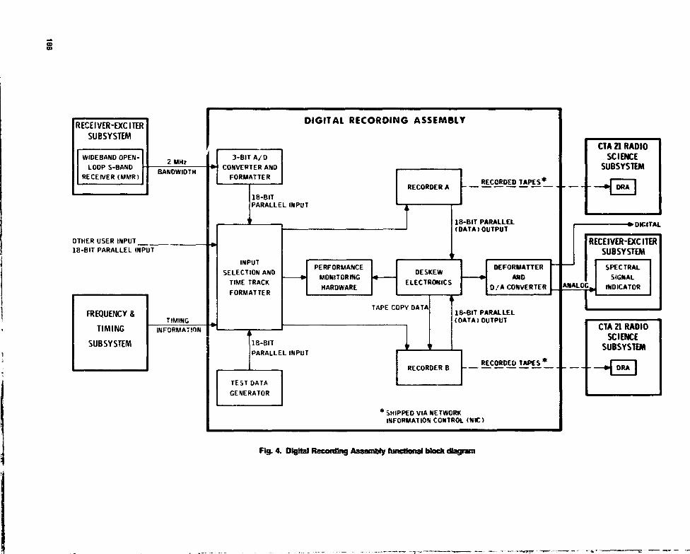
INPUTSELECTION ANDTIME TRACK
FORMATTER
INFORMATION
PERFORMANCEDESKEW
MONITORINGELECTRONICS
HARDWARE
TAPE COPY DATA
DEFORMATTER
AND
D/A CONVERTER
18-BIT PARALLEL(OATA)OUTPUT
18-BITPARALLELINPUT
rmco
RECEIVER-EXCITER DIGITAL RECORDING ASSEMBLY
SUBSYSTEM
WIDEBAND OPEN- 2 MHz 3-8IT A/DLOOP S-BAND
BANDWIDTHCONVERTER AND
RECEIVER(MMR) FORMATTERRECORDED TAPES*
RECORDER A - - - - - - -
18-BITPARALLELINPUT
18-817 PARALLEL(DATA)OUTPUT
OTHER USER INPUT18-BIT PARALLEL INPUT
FREQUENCY &
TIMING
SUBSYSTEM
RECORDER B ^-- RECORDED TAPES
TEST DATA
GENERATOR
SHIPPED VIA NETWORKINFORMATION CONTROL (NIC)
Fig. 4- D " Amy t
CTA 21 RADIOSCIENCE
SUBSYSTEM
DRA
---0 DIGITAL
RECEIVER-D(CITER
SUBSYSTEM
SPECTRAL
SIGNALINDICATOR
CTA 21 RADIOSCIENCE
SUBSYSTEM
ORA

0SN PMWGU ROW 42.44
January and February 1078
N78°24233
Soler Wind Density Fluctuation and the Experiment toDetect Gravitational Waves In Ultraprecise
Doppler DataA. L. Berman
TDA Engineering Office
The experiment to detect gravitational waves in ultrap►ectse Doppler data requires atotal system (DSN Tracking System, spacecraft transponder, and media) fractionalfrequency fluctuation of approximately 1 X 10- 11 for averaging times greater than1000 seconds. At such levels, solar wind density fluctuation loons as a very difficulteiror source.
This article presents a detailed examination of solar wind electron (columnar)density fluctuation as it applies to the experiment to detect gravitational waves inultraprecise doppler data, Expected two-way S-band fractional frequency fluctuation (dueto solar wind density fluctuation) at a 1000-second averaging time is considered to beapproximately 3 X 10- 13, while the optimum two-way X-band (X-band uplink anddownlink) performance is predicted to be (also at a 1000-second averaging time)approximately I X 10' 14 . The article concludes that both two-way S-band and X-bandwill be required (simultaneously) so that the predicted two -way X-band performance(_10- 14) can be improved to a (defined) media goal of 3 X 10 16 via two-way dualfrequency calibration of solar wind induced density fluctuation.
I. IntroductionIn order to utflize two-wa} ultraprecise doppler data in
the attempt to detect and measure various parameters of(hypothesized) gravitational waves (Refs. i and 2), one re-quires a total measurement system fractional frequency fluc-tuation on the order of 10' t s , over the averaging times ofinterest (approximately 50 to 5000 seconds). Major elementsincluded in the total measurement system are:
(1) USN Tracking System.
(2) Media (electron density fluctuation).
(3) Spacecraft transponder.
Since there are multiple elements in the DSN TrackingSystem which independently influence total system perfor-mance, a fractional frequency fluctuation goal of 3 X 10- 16
189

for each (independent) element will be adopted. At the pre-sent time, the two-way' S-band media (solar wind density)fractional frequency fluctuation performance appears to heapproximately 3 X 10- 1 3 (averaging times > 1000 seconds),or 3 orders of magnitude short of the desired 3 X 10- 16level. The steps which need to be taken (higher frequencyband capability, dual frequency band capability) within theDSN Tracking System and oil spacecraft to significantlyreduce media effects may begin to rival those necessary toput the DSN Tracking System on all fractional fre-quency fluctuation basis of less than 10 -1 -5 . Given the int•portance of solar wind density fluctuation in the usage ofultraprecise doppler data for the detection and measurementof gravitational waves, one requires accurate solar wind den•sity fluctuation data for the design and implementation ofsuch an ultraprecise doppler based gravitational wave detec-tion experiment. It is the purpose of this article to presentand analyze treasured solar wind electron density flu tuationperformance, appropriately formatted as fractional frequencyfluctuation. Extensive two-way S-band doppler noise statis-tics acquired from a variety of spacecraft during 1975 and1976 (Refs. 3 through 8) are used to construct average solarwind density fractional frequency fluctuation performance.
II. Solar Wind Density FractionalFrequency Fluctuation Performance
Two-way S-band doppler noise results obtain^d with theViking spacecraft can be summarized (Refs. 5 and 6) as follows:
rof(r)
0] 0'2 9
) = 1.182 X 10⁻³ Q F(a, Q) l J(sin a)t ,s r
where:
o^r) = doppler noise, Hz
a = Sun-Earth-Probe angle, radians
0 = Earth-Sun-Probe angle, radians
r = doppler sample int ;val, seconds
Ra, R) = I - 0.05 (0 - rrl'- + 0) 3 - (a - n /2)3
I a
' For the remainder of this article, "two-way" will specifically :onnote"two-way (coherent) tracking mode, both uplink and downlink at thestated frequency",
190
- 0.00275 ; (Q._°.. 02 + 05 - (a - rrl-)s
The algorith11 2 used to calculate doppler noise (essen-tially) filters out fluctuation frequencies (v) lower than vowhere (Ref. 8):
vo x (30r)-'
Assuming a similar filtering out of (relatively) low frequencyfluctuations in possible gravitational wave data reductionalgorithms3 , the (given) doppler noise expression callrather directly applied to the gravitational wave Detectionproblem, with doppler sample interval approximately equalto averaging tittle.
Selecting if case of the spacecraft -Earth lineperpendicular to the Sun-Earth line (with the spacecraft atinfinity), so (hat:
a = 90°
Q = goo
the doppler noise expression reduces to:
I3
L10J
0,29rr (r) = 1.60 X 10 , liz
which yields a fractional frequency fluctuation (of(r)/1) fortwo-way S-band (uplink and downlink) of':
of*(r)lf'= 2.28 X 10-' 2 r-0.29
Scaling by (3111) 2 , one obtains the equivalent expected two.way X•band performance:
o f(r)lf = 1.70 X 10-'3 r-0'29
2 A "running" standard deviation computed from a least squares linearcurve fit to 15 samples of actual minus predicted (average) dopplerfrequency.
The design and implementation of algorithms to reduce and detectgravitational waves in ultraprecise doppler data will lie it major part ofthe experiment.
ORIGINAL PAGE ISOF POOR QUALITY

Figures I and 2 present average two-way S- and X-band frac-tional frequency fluctuation versus doppler sample interval.
Considering averaging periods of approximately 3 hours("pass average"), Refs. 3, 4, and 6 found the average onestandard deviation of (pass -average) duppler noise (o ) abouta mean geometric value (6,,) established over several monthsof data to be (expressed in terms of 10logtn(on161,)):
a(op /01,) - 1.92 dB (-36%, +56%)
This value is applied as limits to the average fractional fre-quency fluctuation data presented in Figures I through 4.
111. Additional Factors In the Reduction ofSolar Wind Density Fluctuation
Fxpected levels of fractional frequency fluctuation can hereduced somewhat by consideration of three additional cir-cumstances:
( I ) Density variations with solar cycle.
(2) Columnar density minimization in the antisolar direc-!ion (p = 0°).
(3) Columnar density fluctuation to (mean) density ratiominimization in the antisolar direction.
These conditions are briefly discussed below.
A. Density variations with solar CycleIt is shown in Ref. 9 that the ratio of density and density
fluctuation between solar cycle maximum and mini ►ntnn (forSolar Cycle 20) was approximately 0.65 (value at n ► aximun ►divided by value at minimum). The data used to derive theresults of Section II were obtained at Solar Cycle minimum,hence one tr,ight expect to find at the next Solar Cycle (21)maximum (1979- 198 1) a reduction in average fractional fre-quency fluctuation by approximately 0,65.
B. Columnar Density Minimization in the AntieolerDirection (R = 00)
The antisolar direction provide the minimum columnardensity and hence (Ref. 7) the minimum columnar densityfluctuation also. The columnar density reduction betweenthe standard geometry chosen in Section II:
a = 90°
0 _ O0°
and the antisolar direction:
a = 180°
p-0°
Is approximately (assuming an r-` 2 density falloff forr> I AU):
/rr
and hence the density fluctuation can be expected to hereduced by a similar amount. Combination of this reductionwith that from Subsection A yields a total reduction by afactor of 0.414. Figures 3 and 4 present the two-way S- andX-band average fractional frequency fluctuation for theseconditions,
C. Columnar Density Fluctuation to (Mean) DensityRatio Minimization in the Antieolar Direction
Although columnar density (and hence columnar densityfluctuation) is minimized in the antisolar direction, theremay be a further reduction in the columnar density fluctua-tion because of a reduction in the columnar density fluctua-tion to (mcan) density ratio (defined as c', in Ref. 7). Quitesimply, in the a = 90° case, density enhancements propagatingradially cross the signal path perpendicularly near I AU(region of maximum density) with attendant (solar wind)velocities of approximately 440 krn/second, as in Figure 5,As the antisolar direction is approached, the density en-hancement propagation paths line up with signal path, andhence the density enhancements can be expected to moveacross the signal path with greatly reduced velocity (i.e.,shifting the columnar fluctuation spectrum to lower fre-quencies).
The ground tracking system (with Rubidium frequencystandard) duppler noise level for 60-second sample intervaldata is approximately (Ref. 5):
3 X 10_ 3 Hz
while the solar wind density S-band frequency fluctuation inthe antisolar direction is expected to he:
X 10 -_3 Hz
It would therefore not have been previously possible totest this hypothesis (of a further reduction of density fluc-
181

tuation in the andsolar direction). However, with the currenthydrogen maser frequency standard implementation at the64-m subnet and the attendant large reduction in the groundtracking system noise level, it may now be possible to easilytest this hypothesis.
Iv. ConclusionsIwo-way X-band (uplink and downlink), under even the
most optimum conditions, results in a fractional frequencyfluctuation of no better than 10-14 for averaging periods ofat least 1000 seconds. To achieve the goal of 3 X 10° 16, itis here considered that solar wind density fluctuation willhave to be further removed via dual frequency calibration. Itmay be possible to achieve the 1-1/2 orders of magnitude
Improvement from the two-way X-band performance level(_ 10- 14) to the desired level (3 X 10- 16 ) via use of artadditional S-band downlink (only) in combination with two.way X-band; in this regard, Wu, at W. (Fief. 10), have de-veloped sophisticated techniques for calibration of r-,linkrange when dual frequency is only available on the down.link. Hots aver, to more adequately guarantee the requiredimprovement (to 3 X 10- 16) and to substantially reducedata reduction costs (i.e., by not requiring complex calibra-tion algorithms such as the Wu uplink calibration technique)associated with the experiment, it seems reasonable to addi-tionally require two-way S-band. It is thus here concludedthat the implementation of a viable gravitational wave detec.tion experiment based on ultraprecise doppler data will re-quire simultaneous two-way X-band and two-way S-bandcapability.
192

References
1. Thome, K. S., and Braginsky, V. B., "Gravitational-Wave Bursts from Nuclei ofDistant Galaxies and Quasars: Proposal for Detection Using Doppler Tracking ofInterplanetary Spacecraft," in The Astrophysical Journal, Volume 204: LI-L6,February 15, 1976.
2. Estabrook, F. B., and Wahlquist, H. D., "Response of Doppler Spacecraft Trackingto Gravitational Radiation," in Genera/ Relativity and Gravitation, Volume 6,No. 5, 1975.
3. Berman, A. L., and Wackley, J. A., "Doppler Noise Considered as a Function ofthe Signal Path Integration of Electron Density," in The Deep Space NetworkProgress Report 42-33. Jet Propulsion Laboratory, Pasadena, California, 15 June1976.
4. Berman, A. L., Wackley, J. A., Rockwell, S. T., "The 1976 Helios and PioneerSolar Conjunctions — Continuing Corroboration of the Link Between DopplerNoise and Integrated Signal Path Electron Density," in The Deep Space NetworkProgress Report 42.36, Jet Propulsion Laboratory, Pasadena, California, 15 Decem-ber 1976.
5. Berman, A. L., "A Comprehensive Two-Way Doppler Noise Model for Near-Real-Time Validation of Doppler Data," in The Deep Space Network Progress Report42-37, Jet Propulsion Laboratory, Pasadena, California, February 15, 1977.
6. Berman, A. L., Wackley, J. A., "Viking S-Band Doppler RMS Phase Fluctuations Usedto Calibrate the Mean 1976 Equatorial Corona," in The Deep Space NetworkProgress Report 42-38, Jet Propulsion Laboratory, Pasadena, California, 15 April1977.
7. Berman, A. L., "Proportionality Between Doppler Noise and Integrated Signal PathFle.:tron Density Validated by Differenced S-X Range," in Tire Deep Space Net-work Progress Report 42-38, Jet Propulsion Laboratory, Pasadena, California,April 15, 1977.
8. Berman, A. L., "Phase Fluctuation Spectra: New Radio Science Information toBecome Available in the DSN Tracking System Mark 111 .77," in The Deep SpaceNetwork Progress Report 42-40, Jet Propulsion Laboratory, Pasadena, California,August 15, 1977.
9. Berman, A. L., "Deep Space Telecommunications and the Solar Cycle: A Reap-praisal," in The Deep Space Network Progress Report 42-43, Jet PropulsionLaboratory, Pasadena, California, February 15, 1978.
10. Wu, S. C., and Winr, , . B., "A Technique to Determine Uplink Range CalibrationDue to Charged Particles," in The Deep Space Network Progress Report 4241, JetPropulsion Laboratory, Pasadena, California, October 15, 1977.
ORIGINAL PAGE IbOF POOR QUALITY
193

10-1'10 -1IOU 101 10` 10'
wM
bv' 10-12
a
10-i:
a
10-11
°
°
SUN-EARTH-PROBE ANGLE (a) 900
SOLAR CYCLE RATIO = 0,65
AVERAGE VALUE
1 o DEVIATION (+56'1., -36'/.)I
104
DOPPLER SAMPLE INTERVAL, r (SECONDS)
Fig, 1, Two-way 8-bend plasma fluctuation at solar cycle minimum
10-12
SUN-EARTH-PROBE ANGLE (a) 900
SOLAR CYCLE RATIO = 0.65
AVERAGE VALUE
--^ 10- DEVIATION (+56/, -36ry)
H10-13
10-14
o.
10-1'10-110° 101 10` 10'
DOPPLER SAMPLE INTERVAL, T (SECONDS)
Fig. 2. Two-way X-bend plasma fluctuation at solar cycle minimum
104
194

10-11
o- 12
a ^ ^
10-13
SUN-EARTH-PROBE ANGLE (a)= 1800
d SOLAR CYCLE RATIO= 0.65AVERAGE VALUE
1 o DEVIATION (+56'h, -36%110-14
10 -1 100 101 10 2 10 3 104
DOPPLER SAMPLE INTERVAL, T (SECONDS)
Fig. 3. Two-way S-band plasma fluctuation at Solar cycle maximum
10-' `1
a
bM 10-• 3
10 4
SUN-EARTH-PROBE ANGLE W=) = 1800SOLAR CYCLE RATIO= 0.65 ^.
AVERAGE VALUE
— 1 o DEVIATION (+56%, -361/6)10-
10 0101 102 103
4
DOPPLER SAMPLE INTERVAL, T (SECONDS)
Fig. 4. Two-way X-band plasma fluctuation at solar cycle maximum
ORIGINAL PAGE I5
OF POOR QUAUVM19S

a • 180"
OBE ANGLE
NCEMENTS"
Fig. S. Possible reduction In the (columnar) density fluctuation/density ratio In theantieolar direction
196

D8N Progress Report 42 .44 January and February 1978
N78-24234
Solar Wind Turbulence Models Evaluated via Observationsof Doppler RMS Phase Fluctuation and Spectral
Broadening In the Inner CoronaA. L. Berman
TDA Engineering Office
The modelling of doppler noise (RMS phase fluctuation) has en)oyed considerablesuccess via the experimentally observed proportionality between doppler noise andIntegrated electron density. Recently, theoretically derived models for doppler noise havebeen proposed These models are broadly characterized as representing proportionalitybetween doppler RMS phase fluctuation (m) and particle flux. Under the assumptions ofconservation of particle flux in the solar wind and proportionality between electrondensity and electron density fluctuation, these models yield a doppler noise dependenceupon signal closest approach point (a) of.-
0 a a-I.S
Doppler noise observations in the inner corona (r. < a < Sro) are shown toconclusively demonstrate that doppler noise is proportional to integrated electron density(^-a- S ), and not a-' ,5 , as predicted by •he particle flux models. Similarly, spectralbroadening in the inner corona is seen to be proportional to integrated density. Thearticle concludes that the particle flux models are in disagreement with the experimentalobservations of doppler noise to date, end hence are a rlikely to be representative ofactual solar wind processes.
I. IntroductionBerman and Wackley (1976, Ref. 1) have experimentally
demonstrated that doppler noise (RMS phase fluctuation) isproportional to signal path integrated electron density.Recently, other investigators have derived theoretical expres-sions for the radial dependence of doppler noise. Callahan(Ref. 2) has derived such an expression for doppler noise, andWoo (Ref. 3) has both derived such an expression for and
analyzed doppler noise ("Doppler Scintillation"). These inde-pendent efforts have resulted in somewhat similar models,which can be broadly characterized in terms of the depen-dence of doppler RMS phase fluctuation (0) upon signal closestapproach point (a) as:
0 a particle flux • a0. s
197

applying the conservation of particle flux in th_ solar wind andassuming proportional i ty between electron density and elec-tron density fluctuation, one directly obtains:
0a(a- 2).ao.5=a-1.5
This article examines the performance of these models(hereafter to be referred to as the "particle flux models") inrespect to the experimental observations of doppler noise inboth the extended corona (5ro <r< IAU; ro = solar radius,r = radial distance) and inner corona (ro < r,< Sr.) ), andconcludes that the particle flux models are incompatible withthe experimental observations to date. At the same time, thesedoppler noise observations continue to st y .igly support theproportionality between doppler noise and integrated electrondensity (hereafter to be referred to as the "integrates' densitymodel") as espoused by Berman and Wackley.
II. The Particle Flux ModelsEvaluation of Eq. (24) from Callahan (Ref. 2) yields for the
primary term:
0 a n(a)v(a)ao.s
where:
n = electron density fluctuation
v = solar wind radial velocity
If one assumes the conservation of particle flow in the solarwind (Cuperman and Harten, Ref. 4):
K = Nr(r)v(r)r2
where:
N, = electron density
in combination with the common assumption of proportion-ality between electron density and electron densityfluctuation:
N^(r) a n(r)
one directly obtains for doppler noise
0CXW2),ao.5=a-1.5
Simplification of Eq. ('4) from Woo (Ref. 3) yields fordoppler noise:
0 a n(a)lv(a)) s" ao.s
Considering vSf6 At% v (as Ref. 3 does) and assuming conserva-tion of particle flow and proportionality between electrondensity and electron density fluctuation, one immediatelyobtains:
0 as- t.s
By far the most interesting feature of these particle fluxmodels is their absolute insensitivity to the radial dependenceof (integrated) electron density! It is precisely this feature ofthe particle flux models which allows a straightforwardevaluation via comparison to experimental observations ofdoppler noise in the vastly different regimes of the inner andextended corona. Briefly stated, the radial dependence ofelectron density is well known to change from r 6 to r 2.3in the transition from the inner to the extended corona. Theparticle flux models predict that doppler noise will not"detect" this abrupt change in electron density; correspond-ingly, the integrated density model predicts that doppler noisewill exactly mirror the sharp change in electron density.
111. Model Evaluation In theExtended Corona
To date, the only highly precise and mathematicallyobjective determination of the radial dependence of dopplernoise in the extended corona is Berman, Ref. S. This studyfound the radial index to be - 1.30 (a- 1.30), which corre-sponds to a (--, -) integration c..)f r-2.30. Since the averageradial dependence of electron density in the extended coronafound by a variety of experimenters is approximately r-2.3(Ref. 6), the results of Ref. 5 strongly support the integrateddensity model. Figure I (from Ref. 5) shows the results of asimultaneous two parameter least squares minimization to the(extended corona) coefficient and radial index. Althoughobservations of doppler noise in the extended corona asportrayed in Fig. 1 clearly favor the integrated density modelover the particle flux models, the difference between a t •30and a- 1 - 5 is not large in absolute terms, and hence theextended corona results cannot be considered dramaticallyconclusive. Fortunately, the inner corona, with its abrupt shift
198

in the radial dependence of electron density, allows no suchambiguity. The data must conclusively favor one model overthe other.
IW Model Evaluation In the Inner CoronaInner corona electron density observations via both eclipse
photometry methods (van de Hulst, Ref. 7; Saito, Ref. S; andBlackwell, Ref. 9) and spacecraft range delay measurements(Muhlenian (Mariner 6) Ref, 10; Edenhofer (1-lelios 2),Ref. 11) show an extremely sharp change in electron densityradial dependence at approximately r = 4ro . The correspond-ing breakpoint for signal path integrated electron density isapproximately a = 3re. Since the particle flux models areindependent of electron density, one would expect no changeit the doppler noise radial dependence at a = 3ro . Figure 2presents doppler noise observations for the region 2r, <,a<,<,6ro ; included in Fig. 2 is the integrated density model ofBerman (ISEDC) and the particle flux model of Callahan.There is no question but that experimental observations ofdoppler noise in the inner corona "sense" the sharp increase ofintegrated electron density at a - 3ro. To this author it is aninescapable conclusion that the particle flux models simply donot correctly predict experimental observations of dopplernoise, and hence their derivations cannot be consideredrepresentative of actual solar wind processes.
V. Spectral Broadening In the Inner CoronaWoo (Ref. 12) has derived a model for the spectral broadening
(B) of a monochromatic spacecraft signal which is quite similarto the particle flux model of Ref. 3 (actually 0 = B 5/6 fromRef. 3). Therefore, just as for doppler noise, spectral broaden-ing observations in the inner corona should not (according toRef. 12) detect the onset of the inner corona electron densityenhancement. To date, Rockwell (Ref. 13) has performed theonly highly precise and mathematically objective study ofspectral broadening radial dependence in the inner corona.Reference 13 achieved excellen! results in fitting spectral
broadening data via use of a model resembling integratedelectron density. Figure 3 presents the data from Ref. 13;included in Fig.3 are the individual "inner corona" and"extended corona" components from Rockwell's model. Theimportant point is that the two components become equalvalued at a x 3ro , and hence spectral broadening data "sense"the change in electron density exactly as does doppler noise(and quite significantly, at the same radial distance). The clearfact that spectral broadening data are in good agreement withintegrated electron density in the inner corona provides a mostpowerful refutation of the particle flux modelf for both RMSphase fluctuation and spectral broadening.
A Conclusions and DiscussionRecent attempts to theoretically derive the parametric form
of doppler noise have produced ("particle flux") models whichare independent of (integrated) electron density. The innercorona, with its vastly distinct electron density regimes,provides a most powerful test bed to assess the validity of theparticle flux models. Experimental observations of dopplernoise in the inner corona dramatically respond to the abruptchange in electron density regimes, and hence it must beconcluded that the particle flux models do not model actualsolar wind processes. Similarly, observationsspectral broad-ening in the inner corona mirror the doppler noise observa-tions, and hence provide even further fortification of thenegative evaluation of the particle flux models. It is anins ,orable conclusiot, of this article that both RMS phasefluctuation and spectt:A broadening are proportional to inte-grated electron density, and not, as has been suggested,particle flux.
The importance of this conclusion should not be over-looked. With proportionality to integrated electron density,doppler noise represents a most powerful experimental toolfor obtaining the radial dependence of' both electron densityand solar wind radial velocity; were the particle flux modelscorrect, then doppler noise would be far less useful as a radioscience data type.
199

References
I. Berman, A. L., and Wackley, J. A., "Doppler Noise Considered as a Function of theSignal Path Integration of Electron Density," in The Deep Space Network ProgressReport 42.33, Jet Propulsion Laboratory, Pasadena, California, 15 June 1976.
2. Callahan, P. S., "A First-Principles Derivation of Doppler Noise Expected From SolarWind Density Fluctuations," in The Deep Space Network Progress Report 42.42, JetPropulsion Laboratory, Pasadena, California, December 15, 1977.
3. Woo, R., "Radial Dependence of Solar Wind Properties Deduced from Helios 1/2 andPioneer 10/11 Radio Scattering Observations," in The Astrophysical Journal, 219,January 15, 1978.
4. Cuperman, S., and Harten, A., "Some Physical Implications of Recent Solar WindMeasurements," in Solar Wind, edited by Sonett, C. P., Coleman, P. J. Jr., andWilcox, J. M., National Aeronautics and Space Administration, Washington, D.C.,1972.
5. Berman, A. L., Wackley, J. A., Rockwell, S. T., and Kwan, M., "Viking DopplerNoise Used to Determine the Radial Dependence of Electron Density in theExtended Corona," in The Deep Space Network Progress Report 42-38, JetPropulsion Laboratory, Pasadena, California, 15 April 1977.
6. Berman, A. L., "Electron Density in the Extended Corona: Two Views," in TheDeep Space Network Progress Report 42-41, Jet Propulsion Laboratory, Pasadena,California, October 15, 1977.
7. van de Hulst, J. C., "The Electron Density of the Solar Corona," Bulletin of theAstronomical Institutes of The Netherlands, Volume XI, Number 410, February 2,1950.
8. Saito, K., "A Non-Spherical Axisymmetric Model of the Sol-r K Corona of theMinimum Type," Annals of The Tokyo Astronomical Observatory, University ofTokyo, Second Series, Volume XII, Number 2, Mitaka, Tokyo, 1970.
9. Anderson, J. D., Esposito, P. B., Martin, W. L., Thornton, C. L., and Muhleman,D. 0., "Experimental Test of General Relativity Using Time Delay Data fromMariner 6 and Mariner 7," in The Astrophysical Journal, Volume 200, August 15,1975.
10, Muhleman, D. 0., Esposito, P. B., and Anderson, J. D., "The Electron Density Profileof the Outer Corona and the Interplanetary Medium from Mariner 6 and Mariner 7Time Delay Measurements," The Astrophysical Journal, 211, February 1, 1977.
11. Edenhofer, P., Esposito, P. B., Hansen, R. T., Hansen, S. F., Lueneburg, E., Martin,W. L., and Zygielbaum, A. 1., "Time Delay Occultation Data of the HeliosSpacecrafts and Preliminary Analysis for Probing the Solar Corona," in the Journalof Geophysics 42, 1977.
12, Woo, R., Yang, F., and Ishimaru, A., "Structure of Density Fluctuations Near theSun Ded`sced from Pioneer-6 Spectral Broadening Measurements," in The Astro-physical Journal, Vol. 210, No. 2, December 1, 1976.
13. Rockwell, S. T., "An Empirical Spectral Bandwidth Model for Superior Con-junction," in The Deep Space Network Progress Report 42 .43, Jet PropulsionLaboratory, Pasadena, California, 15 February 1978.
200

W
1.0
OO
0.5
10.0
5.0
2.0
0.2
1.6700 C - RADIAL INDEX(,-I- C
COEFFICIENTAO mobervod (I)
a = RMS OF LOGARITHMIC RESIDUALS (10 (on 10model (I)
1.6500
^ 1.6400 F
1.6300
1.6200
0
5.081" 1 ' S o
(CALLAHAN -REF. 2)
Op 4.75 x 10
-109.19 x 10⁻⁵
(SIN a)5(SIN o)1.3
(ISEDC DOPPLER NOISE
MODEL; REF. 5)
ooCD
O
D HELIOS 1O HELIOS 2O VIKING
a = SUN-EARTH-PROBE ANGLE
1.6100 1 1 I 1 1 I 1 _ ,1
.102 .106 .110 .114 .118 .122 .126 .) O
A0 x 102
Fig. 1. Viking 5-Band Doppler noise fit In the extended corona
0.1
1 2 5 10
r, SOLAR RADII
Fig. 2. Doppler noise models In the inner corona
201

oao r'—T'(DATA FROM ROCKWELLREFERENCE 13)
x-99
-lax 10-3 __(SIN a) 1
10^
4.2x 1094.2x1Q3(SIN a) 5 + (SIN a) 1.77
a ° SUN-EARTH-PROBE ANGLE
10—`
1 ` •1 0 :.
1 ^ • •i1 `.•
0.1
0 5 10 's [0
r/r0
Fig. 3. Spectral broadening data In the Inner corona
202

DSN Pr Wn6 Repot 42 .44 January and Fetxuary 1976
On the Suitability of Viking Differenced Rangeto the Determination of Relative Z-Distance
F. B. WinnNavigation Systems Section
Radiometric differenced range residuals (10 Viking orbiting spacecraft observations)have been used to evaluate the current Deep Space Net adopted relative Z distancebetween Deep Space Station 43 and Deep Space Station 14. The Ap noise is approxi-mately twice the predicted noise: ao p is 3.4 in relative to a mean of -1 m. This scatter inthe Ap is most likely due to media calibration uncertainties and Deep Space Net hardwarenoise.
These 10 Ap residuals yield art estimated Z distance between DSS 43 and DSS 14 of7351803.6 m. The standard deviation of that estimate is 10.1 in,
I. IntroductionRadiotnetric differenced range residuals (10 Viking orbiting
spacecraft observations) have been used to evaluate the currentDeep Space Net adopted relative Z distance between DeepSpace Station 43 and Deep Space Station 14, The Deep SpaceNet 'adopted Z coordinates' for Deep Space Stations are aproduct of the Goddard Space Flight Center. The adoptedDSS 43 -DSS 14 relative Z distance is 7.351807 X 10 6 m. JPLhas assigned a 15-in standard deviation to these Z_ coordinates.These 10 Viking differenced range observations, Op, 4o notreveal a relative Z error of statistical significance: the AZcorrection equals 113 the computed ooz. The relative Z cor-rection is -3.4 m and the sigma is 10.1 m. Although this isencouraging, it is not definitive. This range sample is so smallthat systematic effects due to AZ, Deep Space Station longi-tude, and spacecraft declination errors may not have emergedabove the range noiie.
The Ap noise is approximately twice the predicted noise:ao p is 3.4 in relative to a mean of -1 m. This scatter in the Apis most likely due to media calibration uncertainties and DeepSpace Net hardware noise. Additionally, the influences of AZ,Deep Space Station longitude, and spacecraft declinationerrors on Ap are discussed.
II. The Differenced Range Data Set fromthe DSS 43—DSS 14 Baeeline
Near simultaneous range measurements were obtained fromthe DSS 43- DSS 14 baseline (Ref. ?, Ref. 3): seven at anS•band frequency and three at an X-band frequency. The USNacquired these observations from Viking-Mars orbiting space-craft front January to April 1977 in a dual-station rangingdemonstration. Usually only minutes separated the measure-ments of different DSSs (Figs. 1 -6).
203

The positions and velocities of a spacecraft in the solarsystem are estimated usually by a least squares, differentialcorrection technique (Orbit Determination Program, Ref. 4).The Doppler shift experienced by round-trip radio transmis-sion from the earth to the spacecraft and back is the primeobservable used In the least squares technique. A part of theprocedure computes the difference between the observedrange and the range computed from numerical integrations ofrite equations of motion of all the significant solar systembodies.
When compressed range residuals are computed from theraw range residuals (Fig. 1-6) and differenced, the compresseddifferenced range residuals do not show any systematic signa•tures In time (Fig. 7) or as a function of declination (Fig. 8).In these figures, a label of'S' or'X' indicates the frequency ofthe observation and the bar specified the one-sigma dispersionof each Op value. As previously stated, the dispersion of thecombined 'S' and 'X' frequency cp is 3.4 in a mean of-1 m. Alone 'S' band Ap has a o00 = 2.6
in a mean of
-1 m.
III. Additional Australia—GoldstoneBaseline Data
Besides these 10 Ap observations, 4 additional Ap observa-tions were ol-tained from 3 different Canberra—Goldstonebaselines: one from the DSS 42—DSS 14 baseline on 31January; two from the DSS 43—DSS I I baseline on 31 Janu-ary and 16 February; and one from the DSS 42—DSS 11baseline on 16 February.
Geodetic surveys within the Goldstone DSN complex havedetermined the relative Z(OZ) for the short baselines to <1 m(a). The same is true for the DSS of the Canberra complex.Thus, all long baselines between the Canberra and Goldstonecomplexes should have a nearly common AZ error. Although aplot of all 14 Ap points for the Canberra—Goldstone baselinesis consistent with this view, the noise level is so high (a oP =4.1 m) that little weight is given to this observation. Todramatize the noise level of this data, Fig. 9 exhibits what thesignature in Ap from an error in AZ (equal to 18 m, 3 timeswhat the Voyager project specified as acceptable, Ref. 5) lookslike.
IV. Error Analysis for OpThis scatter in the Ap values is most likely due to the
'media' calibration uncertainties (plasma, ionospheric ion, andatmospheric refraction calibration uncertainties) and DSN
ranging system hardware perturbations. It can be shown thatAp scatter Bern in Fig.9 does not stem from geometricalparameters, such as: relative Z distance (AZ)-, Mars declination(b); DSS distance off the earth's spin axis (r,); or, DSS longi-tude errors. Consider the following discussion.
The topocentric range from a DSS to a distant spacecraftmay be approximated (Ref. 6) by
p(t) = R(t) - Z sin b(t) - rj cos b(t) cos (wt - a(t) + AJ
where
p(t) - the topocentric range at time 't'
R(t) - geocentric range
Z n distance of DSS from earth's equator
b - spacecraft declination
r, - distance of DSS from earth's spin axis
w n earth rotation rate
A = DSS longitudea - spacecraft right ascension
For differenced range from two DSS, which aretime synchronized
P2 - p i _ (Z I - Z2 ) sin b
- (r,z - rJ ) cos b (cos (wt - (k) {cos X2 - cos A I )
+ sin (wt - o) (sin A i - sin A2)j
The errors in the differenced range per unit error in 17, Ab,ar,, and A are then
F = sin be(AZ)
F("p) _ AZ cos 8 + Ars sin b [cos (wt - a) {cos X 2 - cos X i }C(AS)
+ sin (wt - (d) {sin A I - sin A 2 )J
204
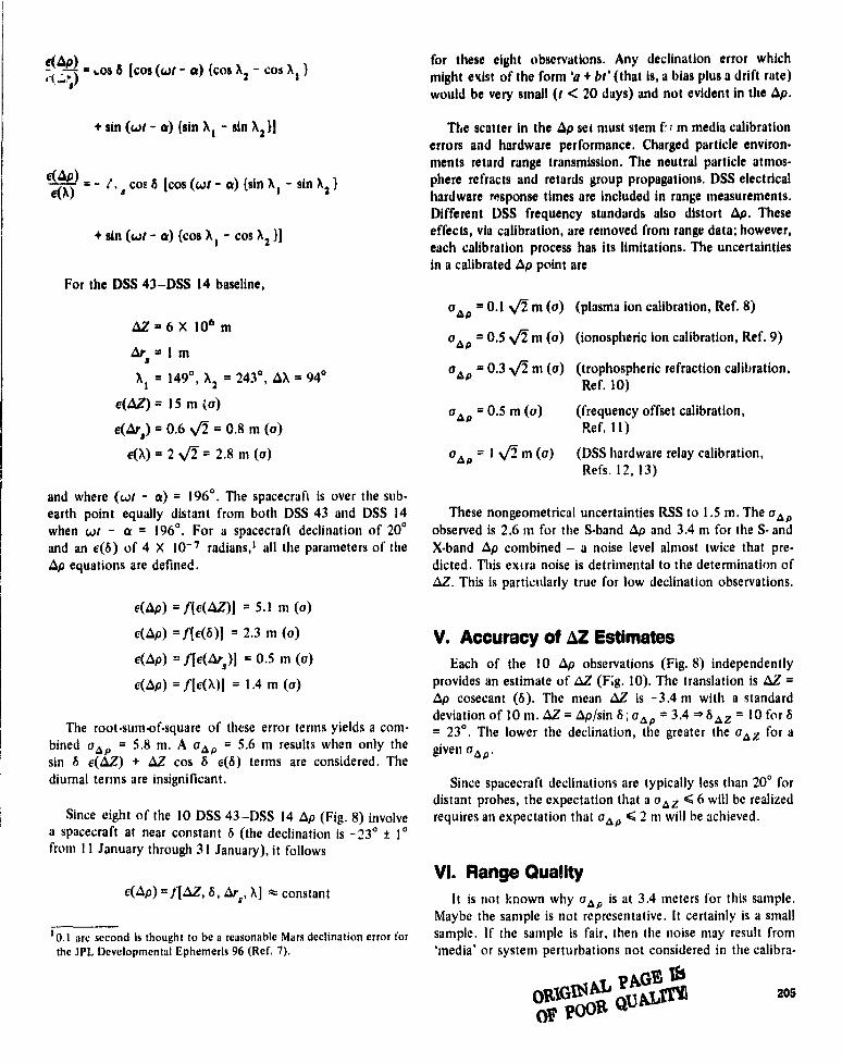
O^ _ -.05 b (cos (Wt - a) (cos X 2 - cos A t )for these eight observations. Any declination error whichmight exist of the form 'a + bt' (that is, a bias plus a drift rate)would be very small ( t < 20 days) and not evident in the Ap.
+ sin (Wt - a) (sin A t - sin X2 )]
4 a - !, a COE b [Cos (Wt - a) (sin A l - sin X2 )
+ sin (Wt - a) (cos A t - cos A2 )]
For the DSS 43—DSS 14 baseline,
AZ = 6 X 10⁶ m
ar =ImsX t = 149 0 , X2 = 2430 , AX = 940
c(AZ) = 15 m (a)
e(Ars) = 0.6 f = 0.8 m (a)
e(X)=2NF2=2.8m(a)
and where (Wt - a) = 1960 . The spacecraft is over the sub-earth point equally distant front DSS 43 and DSS 14when Wt - or 1960 . For a spacecraft declination of 200and an e(b) of 4 X 10⁻⁷ radians,' all the parameters of theAp equations are defined.
e(AP) = ACW)] = 5.1 in (a)
c(OP) = fle(b)] = 2.3 m (a)
c(Ap) = f[e(A?^)j = 0.5 in
e(OP) = fle(X)l = 1.4 m (a)
The root -sutnof-square of these error terms yields a com-bined oo p = 5.8 m. A cro p = 5.6 in when only thesin b c(AZ) + LZ cos b c(b) terms are considered. Thediurnal terms are insignificant.
Since eight of the 10 DSS 43—DSS 14 Ap (Fig. 8) involvea spacecraft at near constant b (the declination is -23 0 t 10froth I 1 January through 31 January), it follows
OAP) = f[AZ, b , ArS , X] ^Zz constant
' 0.I are second is thought to be a reasonable Mars declination error forthe JPL Developmental Ephemeris 96 (Ref. 7).
The scatter in the Ap set must stem P, in calibrationerrors and hardware performance. Charged particle environ-ments retard range transmission. The neutral particle atmos-phere refracts and retards group propagations. DSS electricalhardware r"ponse times are included in range measurements.Different DSS frequency standards also distort Op. Theseeffects, via calibration, are removed from range data; however,each calibration process has its limitations. The uncertaintiesin a calibrated Ap point are
aop = 0.1 f in (plasma ion calibration, Ref. 8)
aop = 0.5 f m (a) (ionospheric ion calibration, Ref. 9)
aop = 0.3 N/2- m (a) (trophospheric refraction calibration,Ref. 10)
oop = 0.5 m (a) (frequency offset calibration,Ref. 11)
oop = 1 \/2 m (a) (DSS hardware relay calibration,Refs. 12, 13)
These nongeometrical uncertainties RSS to 1.5 m. The aopobserved is 2.6 m for the S-band Ap and 3.4 in the S- andX-band Ap combined — a noise level almost twice that pre-dicted. This extra noise is detrimental to the determination ofAZ. This is particularly true for low declination observations.
V. Accuracy of OZ EstimatesEach of the 10 Ap observations (Fig. 8) independently
provides an estimate of oZ (Fig. 10). The translation is VZ =Ap cosecant (b). The mean 6Z is -3.4 in a standarddeviation of 10 m. AZ = Ap/sin b; ao p = 3.4 - boZ = 10 for b= 230 . The lower the declination, the greater the a0Z for agiven aop.
Since spacecraft declinations are typically less than 20° fordistant probes, the expectation that a ao Z < 6 will be realizedrequires an expectation that ao p < 2 m will be achieved.
VI. Range QualityIt is not known why ao p is at 3.4 meters for this sample.
Maybe the sample is not representative. It certainly is a smallsample. If the sample is fair, then the noise may result from'media' or system perturbations not considered in the calibra-
pAGU lbaosOFI
0 pooR QUA
tion process. The media' calibrations do not appear a likelyexplanation. Charged particle calibrations for radiometricrange and Doppler have been compared front such indepen-dent sources as Faraday polarimeter measurements (Ref. 9), S-and X-band dispersive Doppler and range measurements(Ref. 10), and S- and X-band DRVID measurements and foundconsistent to a few lentils of meters. Similarly, troposphericrefraction calibrations consistently yield conventional trackingdata modelled to the 2 to 3 decimeter level. This is true evenfor observations below a 1O0 elevation angle (Ref. 10).
More Ap data will provide the base needed to characterizethe dependence of Ap oil and c(b).
Differenced range data is being acquired from the Voyagerspacecraft while the spacecraft are in heliocentric cruise.Although only tour observations have been processed at thistime, the Voyager Ap appear even noisier than those ofViking. DSN and Voyager personnel are currently investigating
the DSS fundamental calibration procedures in all toreduce the differenced range noise.
Vli. Conalfueions
DSN radiometric differenced range has been used to differ-entially correct the DSS 43- DSS 14 baseline relative Z dis-tance. A correction of -3 in is indicated. However, the stan-dard deviation of that correction is 10 in. Thr prior relative Zsigma was 15 nt. The Voyager project requires a sigma of G in.
The 10 in sigma on relative Z stems from the differencedrange noise (oo p = 3.4 in), the low t.^clination angles for thespacecraft used (S < 25 O ), and transmission media calibrations.
For 6 < 200 , the Ap must have a oo p < 2 in if relative Zdeterminations to standard deviations of less than six metersare to be realized.
206

References
I. Kirsh, J, G.. "A Glohal Station Coordinate Solution Based Upon Camera and LaserData CSFC 1973," presented at the First International Symposium (for) the Useof Artificial Satellites for Geodesy and Geodymamics, Athens, Greece, May 14 21,1973-
2. Christensen, C. S., Green, I). W., Siegel, Ii. L., and Winn, F. B., "Dual StationRanging Demonstrations," EM 314 . 141, Jet Propulsion laboratory, Pasadena, Cali f.,October 27, 1977 (JPL internal document).
3. Siegel, II, L_., Christensen, C. S„ Green, D. W., and Winn 1. B., "On AchievingSufficient Dual Station Range Accuracy for Deep Space Navigation it Zero Declina-tion," presented at AAS/AIAA Astrudynamics Specialist Conference, Jackson Hole,Wyoming, September 7 c), 1977.
4. Moyer, T. C., Alathernatica/ Formulration of the Double Precision Orbit Determina-tion Program (DPODP), TR 32-1527, Jet Propulsion Laboratory, Pasadena, Calif., 15May 1971.
5, Support Instntmentation Requirements Document. NASA, 111) 618-501, NationalAeronautics and Space Administration, Washington, D.C., June 1, 1976, pg. 2116 2.
6. Curkendall, D. W., and Ondrasik, V. J., "Analytic Methods of Orbit Determination,"AAS/AIAA Astrodynamics Conference, Vail, Colorado, July 16 18. 1973.
7. Standish, E. M., etal., R1. De ► elopment Ephemeris Numhe►• 96, TR 32 . 1603, ,letPropulsion Laboratory, Pasadena, Calif., February 29, 1976.
8. Callahan, P. S., "Expected Range and Doppler Differences fur Two•Siation Track-ing," 10M .315.1 . 134, Jet Propulsion laboratory, Pasadena, Calif.. May !6, 1977(Jil l, internal document).
9. Yip, K. W., Winn. F. B., Reid, M. S., and Stelzried. C. T., "Decimeter Modeling ulIonospheric Columnar Electron Content at S-Band Frequencies, ,, I'M 391-620 .letPropulsion Laboratory, Pasadena. Calif., February 7, 1975 (JPL internal document).
10. Madrid, G. A., et , al., t racking S rvsw ►n ; t nalvtic C'alihrcttion Aetiw.'ries for the AlarinerAlars 1971 Alission, Technical Report 32 . 1 SS7, Jet Propulsion Laboratory, Pasadena.Calif., March 1, 1974.
11. Chao, C. C., "Preliminary Report of Differenced Doppler Determination of StationFrequency Offset for Ranging Demonstration," IOM .314.7 . 102, Jet PropulsionLaboratory, Pasadena, Calif., July 28, 1977 (JPL internal document).
12. Spradfin, G. L., "DSS Range Delay Calibrations: Cu rrent Performance Level," DeepSpace Network Progress Repo ►•! 4'-30, pp. 138, Jet Propulsion Laboratory. Pasa-dena, Calif., Ocioher 1976.
13. Koch, 11. E., Chao, C. C., Winn, F. B., and Yip, K. W., "Conditioning of MVM'73Radio-Tracking Data," presented :it AIAA Mechanics and Control of Flight Confer-ence, August 5 c), 1974.
207
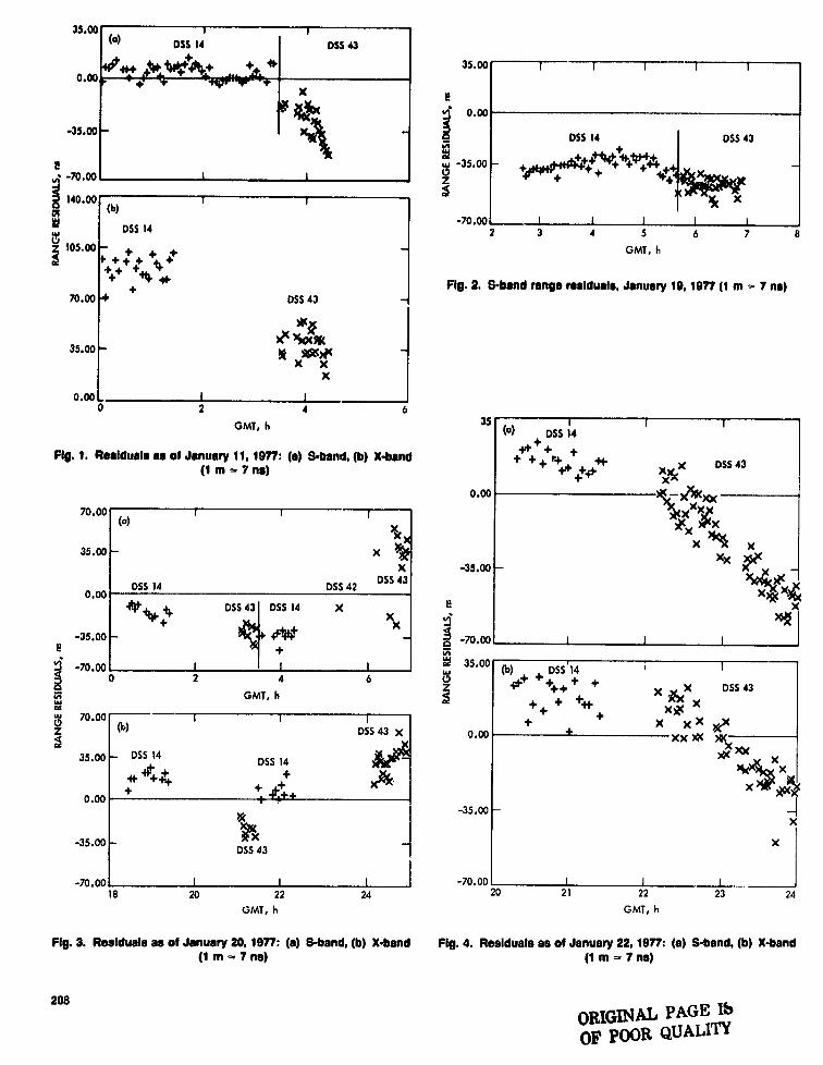
(0) DSS 14 DSS 43
0.00 + m.N+ 1;;4+ + 35.00
X r
> ^ 0.00
-33.00- 1K. DSS 14 DSS 43
1! Lw -35.00 + +; +llm} +• -70.00 g " + #+
140.00 (b)
-70.00
Uy DSS 14 2 3 4 5 6 7 8z 105.00 GMT, h
++ + #+++++ +4k
+ Fig. 2. &bend range residuals, January 19, 1977 (1 m > 7 no)70.00 DSS 43
Wif
35.00 Ust
X
0.00 LI 1
0 2 4 6
GMT, h 35 (°) DSS 144+++ +Fig. 1. Residuals as of January 11, 1977: (a) S-band, (b) X-band + ++ r++ + x x DSS 43(I m - 7 no)
0.00
X X XX70.00 (o) x
^xxXXxX )10^ ,,x
35.00 X
xx X)x -35.00
X)x X4
0.00DSS 14 DSS 42 DSS 43
* DSS 43 DSS 14 X t?X
-35.00 + ^+'^+ -70.00X
c + vi
9a
V) GMT, h g +++ + +9! ++ + * X% X
-70.00 0 2 4 6
^ 35.00 (b) + + DSS 14
70.00
Z DSS 43
o.00 xx sac Vs+ + x xx 0
x *XX
roc35.00
XX
X
0.00-35.00 -I
X
-35.00
X
-70.00 -70.0018 20 22 24 20 21 22 23 24
GMT, h GMT, h
Fig. 3. Residuals as of January 20,1977: (a) S-band, (b) X-band Fig. 4. Residuals as of January 22, 1977: (a) S-band, (b) X-band
(1 m - 7 no) (1 m - 7 ns)
208
ORIGINAL PAGE Ib
OF POOR QUALITY
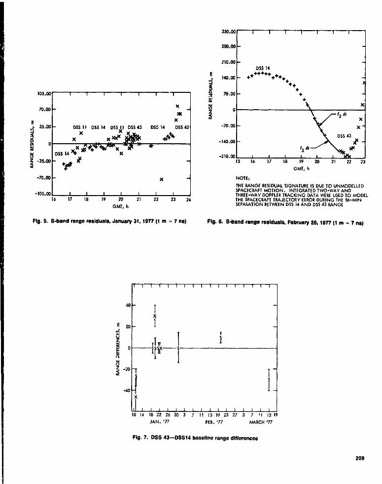
,uv 1 1 1 T
,00
00DSS 14
00 ++++++++++++
++
00 ++
\ f2 dlX
00 X
DSS 4300
f3 d1 1^C
15 16 17 18 19 20 21 22 23
350
280
210
t'140
70WOC
V
-70
-140
-210
00x _)x
X00 DSS 11 DSS 14 DSS X11 DSS 43 DSS 14 DSS 42
X
X
X wxOX
0
XDSS 14 xF X #+ XX00 + ,+ R"
00 I X
00
16 17 18 19 20 21 22 23 24
GMT, h
Fig. S. S-bend range residuals, January 31, 1977 (1 m — 7 no)
GMT, h
NOTE:
THE RANGE RESIDUAL SIGNATURE IS DUE TO UNMODELLEDSPACECRAFT MOTION. INTEGRATED TWO-WAY ANDTHREE-WAY DOPPLER TRACKING DATA WERE USED TO MODELTHE SPACECRAFT TRAJECTORY ERROR DURING THE 56-MINSEPAkAT1ON BETWEEN DSS 14 AND DSS 43 RANGE
Fig. O. S-band range residuals, February 20, 1977 (1 m - 7 no)
105
70,
35
-70,
-105.
40
20NU
0
nW0d
-20
1X1
T
I
10 14 18 22 26 30 3 7 11 15 19 23 27 3 7 1 1 15 19
JAN. '77 FEB. '77 MARCH '77
Fig. 7. DSS 43—OSS14 baseline range differences
209

0
5 Jx1
Ts1
0
S 1S
.5 1x
10
Ead
10
8
6
4
2
Ea 04
2
-40 -30 -20 -10 0DECLINATION, dog
Fig. 8. Jp as a function of declination
142_,1
4
43-11
1x1 -OZ sln842-14
AZ ° 18 mTS1
4p3-11Y
T
6
e x+ AZ sin 8 ;
AZ-18m0
-40 -30 -20 -10 0
DECLINATION, dog
Fig. 9. All %p from Canberra—Goldstone Baselines
-23 -22 -21 -20 -19 -18 -17 -16 -15 -14 -13DECLINATION, dog
Fig. 10..1Z estimates for DSS 43—DSS 14 baseline
1614 T
1
12 1
8
4
E 0N -44
-8
-12
-16
-20
210

DSN Progress Report 42.44 January and February 1978
N78-24236
CCIR Papers on Telecommunications forDeep Space Research
N. F. deGroot
Telecommunications Systems Section
Three papers on telecommunications for deep space research have been adopted by.Study Group 2 of the International Radio Consultative Committee (CCIR). In this article,we present the paper that considers the sharing of radio frequency bands between deepspace research and other radio service.
I. IntroductionStudy Group 2 of the International Radio Consultative
Committee (CCIR) is concerned with the technical aspects oftelecommunications for space research and radio astronomy.Three JPL papers on deep space research were submitted bythe United States for consideration at a meeting held inGeneva during September, 1977. The papers were adopted andare:
Doc. 2/296 Telecommunication Requirements for Mannedand Unmanned Deep Space Research
Doc. 2/269 Preferred Frequency Bands for Deep SpaceResearch Using Manned and UnmannedSpacecraft
Doc. 2/279 Protection Criteria and Sharing ConsiderationsRelating to Deep Space Research
The first of these papers was included in the September-October 1977 issue of the Deep Space Network ProgressReport. Also in that report was a description of the role ofCCIR papers in the establishment of worldwide regulationsthat determine the use of the radio frequency spectrum.
The paper on preferred frequency bands was included inthe November-December 1977 issue.
This article presents the third paper, which considers inter-ference protection and hand sharing with other users.
211

Documents
Doc. 2/279-ECCIR Study Groups
23 September 1977
Period 1974-1978Original; English
UNITED STATES OF AMERICA
Draft New REPORTePROTECTION CRITERIA AND SHARING CONSIDERATIONS
RELATING TO DEEP SPACE RESEARCHrat Quest on Rev.
1. Introduction
This report considers the sharing of frequency bands in the range 140 GHzbetween deep space research stations and stations of other services. Deep space earthand space station protection criteria are discussed. Potential interference is considered,and conclusions are drawn about the feasibility of sharing.
The 1-20 GHz range includes current allocations applicable to deep space researchand some of the frequencies desired for future operational use. Preferred frequencies aregiven in Doc. 2/ 168. U.S. earth and space station characteristics are given in Doc. 2/167.
2. Earth station factors pertinent to sharin
The principal earth station parameters which pertain to interference and sharing aretransmitter power, antenna gain and pointing, receiver sensitivity (including noise tempera-ture) and bandwidth. Typical values of theme parameters are given in Doc, 2/167. Thissection of the report considers some aspects of antenna pointing, and develops protectioncriteria for receivers at deep space earth stations. The section finishes with remarks aboutcoordination. Consideration of transmitter power are given in a later section.
2.1 Intersections of satellite orbits and antenna beams from deep space earth stations.
The locations of the US deep space earth stations are given in Doc. 2/167. Thestations are spaced approximately equally in longitude (120° apart) with two stations in thenorthern hemisphere, and the third in the southern hemisphere. Spacecraft in deep spacecurrently remain in or near the plane of the ecliptic, which is tilted at 23-1/2° from theEarth's equatorial plane. The daily rotatioh of the Earth causes the antenna beam of at leastone earth station to intersect the equatorial plane and hence the geostationary orbit whentracking a given spacecraft. The earth station may be subjected to interference from satel-lites within the antenna beam and operating in or near the allocated deep space bands.
Satellites that are not geoetationary can pass through the one or more deep spacetracking teams each day. Details of visibility statistics and in-beam duration times are con-tained in draft Report AH/2.
In the future the United States plans to deliver deep space probes into o ,.-bits out ofthe plane of the ecliptic. These missions will also result in some earth station trackingbeams passing through the orbits of both geoetationary and non-geoetationary satellites.
2.2 Susceptibility of deep space earth station receivers to interference
A deep space telecommunication system is typically a phase-sensitive system. Theearth station receiver utilizes phase-locked loops for carrier tracking and da a recovery.CW or noiselike interference in these loops can result either In degradation or loss of track-ing and data. Report 544 contains information on the effects of interference In phase-lockedloops. Report 545 presents information on the degradation of telemetering performancecaused by interference.
4, Proposed replacement for Report AL/2
212
PAGE IbORIGINALOF POOR QUALI'

_2.
2.2. l CW signal interference
2.2. 1. 1 Receiver capture. The changing Doppler shift of a received desired signal can causethe receiver pass band to move past a fixed frequency unwanted CW signal. Depending uponrate of motion and the amplitude of the unwanted signal, the receiver may lock to the inter.fering signal if R, the ratio of the CW signal power to the desired signal power, satisfies therelation:
R> df(i)
ofn
where df is the rate of frequency change in Hz/s and fn 1s the loop natural frequency in Hz.
An interfering CW signal that is 10 dB above a strong signal and is moving throughthe receiver passband at 100 Hz/s would cause the receiver to luck to the interfering signal.At a lower rate of movement, the required interfering signal level is proportionately loweruntil at a signal-to-interference ratio greater than one, the interfering signal will no longercapture the receiver, even if the movement rate is zero. Undesired CW signals not strongenough to cause receiver capture may cause interference to carrier tracking.
L.2. 1.2 Carrier tracking degradation. An interfering CW signal can induce a phase modula-tion on the desired carrier signal when the frequency separation between the two signals iscomparable to or less than the phase locked loop bandwidth. A maximum acceptable phasemodulation of loo amplitude results from an interference-to-carrier power ratio of -15 dB.The design margin for carrier tracking is typically 10 dB with reference to the noise powerin the carrier tracking loop bandwidth. For maximum acceptable carrier tracking degrada-tion, the power in a CW interfering signal that may be within the phase locked loop bandwidthmust not be greater than the amount shown in Table I.
TABLE I
CW interference with carrier tracking
Frequency Noise in 1 Hz Loop Minimum Carrier Power Maximum CW Interference
(GHz) (dBW) (dBW) (dBW)
2.3 -216.6 -206.6 -221.6
8.5 -215.0 -205.0 -220.0
15.0 -213.4 -203.4 -218.4
2.2.1.3 Telemetering degradation. Telemetering degradation is defined as the amount bywhich the signal-to-noise ratio must be increased to make the bit error rate, when an inter-fering signal is present, equal to what it would be if the interfering signal was absent. Themaximum allowable degradation for deep space telemetering is 1 dB. For coded telemeter-ing with a threshold signal-to-noise ratio of 2.3 dB, CW interference 6.8 dB below t': noisepower will result in 1 dB degradation. For ur,coded telemetering with a threshold signal-to-noise ratio of 4.8 dB, CW interference 5 .iti below the noise will result in I dB degradation.The noise power is proportional to the data bandwidth and the receiver noise spectral density.Examples of allowable level of CW interference are shown in Table II.
213

.3.
TABLE It
CW Interference with telemetering
Frequency Noise Power in Data Interference-to- Noise Maximum CW
(GUN)Data (bits/s) Bandwidth (dBW) Ratio for i dB Interference
Degradation (ciB) (dBW)
2.3 40, uncoiled -200.6 -5.0 -205.6
8.4 40, coded -200.0 -6.6 -206.8115k, coded -164.4 -6.8 -171.2
15.0 40, coded -197.4 -6.8 -204.2115k, coded -162.8 -6.8 -169.6
2.2.2 Wideband interference
Wideband signals or noise that reduce the signal-to-noise ratio affect both the car-rier tracking and the data channels. In the case of the telemetering channel, the spectraldensity of the interfering signal must be at least 5.9 dB below the spectral density of thereceiver noise in order not to degrade the threshold performance by more than 1 dB. Maxi-mum levels of wideband interference are shown in Table III.
TABLE III
Wideband interference with telemetering
Frequency Noise Spectral Density Interference-to- NoiseMaximum Wideband
Interference(GUIZ) (dB(W/Hz)) Ratio (dB) (dB(W/l-lz))
2.3
8.415.0
-216.6
-215.0
-213.4
.5.9
-5.9-5.9
-222.5
-220.9
-219.3
2.2.3 Interference to maser operation
Mixing of signals with the idler frequency of the maser pump can cause interferenceand saturation in the receiver pasaband. There are many frequencies at which such mixingcan occur, all of which are far removed from the normal frequency of reception. Table IVgives possible interference frequencies for the two frequency bards currently used for recep-tion at deep space research earth stations.
Interfering signals must be above -120 dBW in the idler bandwidth (which is verybroad) at the maser input to be significant.
TABLE IV
Frequencies at which interference may be caused by mixing in the maser
Receiver frequency band 2 290 - 2 300 MHz 8 400 - 8 500 MHz
Maser pump frequency 12.7 Gliz 11).3 and 24.0 Gl-lz
Interference frequencies 15.0 G11z 32.4 GHz10.4 27.87.5 15.65.2 10.9
2.2.4 Adjacent channel receiver saturation
The -ryogenically cooled maser of the deep space receiver has a bandpass of approximately 50 Mliz. Adjacent channel signals, if received at total power levels greater than
214
ORIGIN' PAGEOF POUR QUAL1a
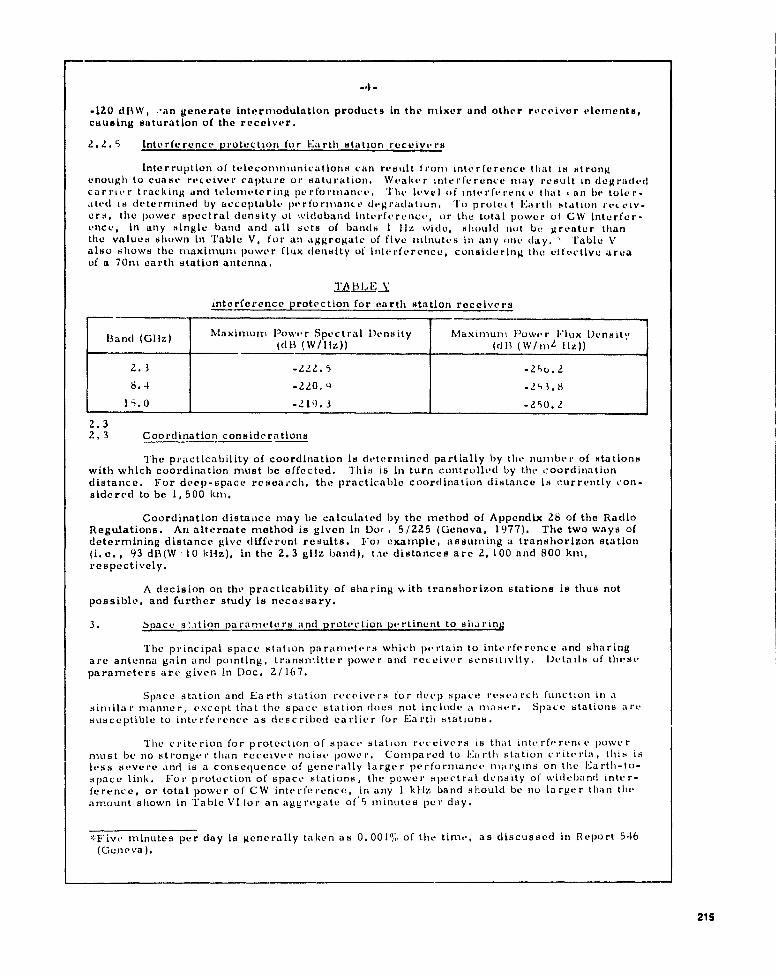
.4.
-120 d13W, . , an generate intermodulation products In the mixer and other receiver elements,causing saturation of the receiver.
2.2.5 Interference protection for Earth station receivers
Interruption of telecommunications can result from interference that is strongenough to cuase receiver capture or saturation. Weaker trite rference may result in degradedcarrier tracking and telemetering performance. The level of interference that can be toler-ated is determined by acceptable performance degradation. To protect Earth station receiv-ers, the power spectral density of wideband interference, or the total power of CW interfer-encc, in any single band and all sets of bands 1 liz wide, should nut bat greater thanthe values shown In Table V, for an aggregate of five minutes In any .rite day. fable Valso shows tilt , maximum power flux density of interference, considering the effective +:treatof a 70m earth station antenna.
TA t3L ? Vinterference protection for earth station receivers
Band (Gliz) Maximum flower Spectral Density Maximum Flower Flux Densityldli (W/110) (dB (W/n, 2 llz))
2.3 -222.5 -256.28.4 -220.9 -2113.8
75.0 -210.3 -250.2
2.32, 3 Coordination considerations
The practicability of coordination is determined partially by the number of stationswith which coordination must be effected. This is in turn controlled by the coordinationdistance. For deep-space research, the practicable coordination distance is currently con-sidered to be 1, 500 kni.
Coordination distance may be calculated by the method of Appendix 28 of the RadioRegulations. An alternate method is given in Doc- . 5/225 (Geneva, 1977). The two ways ofdetermining distance give different results. For example, assuming a transhorizon station(I. e., 93 dB(W r 10 kliz.), in the 2.3 gHz band), t,te distances are 2, 100 and 800 km,respectively.
A decision on the practicability of sharing with transhoriron stations Is thus notpossible, and further study is necessary.
Space s'.rtion parameters and protection pertinent to sharing
The principal space station parameters which pertain to interference and sharingare antenna gain and pointing, transmitter power and receiver sensitivity. Details of theseparameters are given in Doc. 2/167.
Space station and Earth station receivers for deep space research function in asimilar manner, except that the space station does not include a maser. Space stations aresusceptible to interference as described earlier for Earth stations.
The criterion for protection of space station receivers is that interference powermust be no stronger than receiver noise power. Compared to Earth station criteria, this ieless severe and is a consequence of generally larger performance niargins on the Earth-to-space link. For protection of space stations, the power spectral density of wideband inter-ference, or total power of CW interference, in any 1 kiiz band should be no larger than theamount shown in Table Vlfor an aggregate of 5 minutes per day.
,: , Five minutes per day is generally taken as 0.001°,, of the time, as discussed in Report 546(Geneva).
215

-5-
TABLE VIInterference krotection for mace station receivers
Frequency (Gliz) Maximum Interference Level (dB(W/kllz))
2.1 -170.8
7.2 -16,0.615.0 -168.1
Space station e. I. r, p, is normally reduced while near Earth, minimizing the poten-tial for interference to other stations.
4. Sharing considerations
The following paragraphs consider the possibility of interference between deupspace research stations and those of other services. There are 8 possibilities to be con-sidered, as shown in Table VII.
Table VII and the following paragraphs consider the possibility of interference,inthe deep space research Earth-to-space bands.
TABLE VIIPotential Interference in Earth-to-space bands
Source Receiver
Earth station Terrestrial stationEarth station Near Earth satellite
Terrestrial station Earth stationTerrestrial station S; ;.:e station
Space station Terrestrial stationSpace station Near Earth satellite
Near Earth satellite Earth stationNear Earth satellite Space station
4.1 Potential interference to terrestrial receivers from earth station transmitters
The normal maximum total power for current U.S. earth stations is 50 dBW. Fora typical minimum elevation angle of 10 degrees, the e. i.r. p. directed towards the horizondoes not exceed 57 dB(W /4 khlz), assuming the reference earth station antenna radiationpattern of Recommendation AA/2. For spacecraft emergencies, the maximum total powermay be increased to 56 d13W, giving not more than 63 dB(W/4 kHz ► at the horizon. Thesevalues of e. I. r. p. meet the requirements of RR 47OF.
Aircraft stations within line-of-sight of a deep-space earth station will encountertotal power 'lux densities as shown in Figure 1. For an aircraft altitude of 12 km, themaximum line-of-sight distance to an earth station is 391 km and the total power flux densityat the aircraft can never be lower than -83 dB(W/m ), again assuming the antenna pattern ofRecommendation AA/2. Depending on distance and earth station antenna direction, the air-craft station may experience much higher flux densities and interference levels. Coordina-tion with airborne stations is generally not practicable.
216
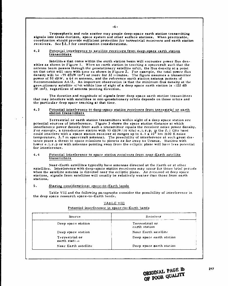
.6-
Tropospheric and rain scatter may couple deep-space earth station transmittingsignals Into trans - horizon, space system and other surface stations. When practicable,coordination should provide sufficient protection for terrestrial receivers and earth stationreceivers. See 12.3 for coordination considerations.
4. Z Potential Inte rference to satellite receivers from deep -space earth station
tranrn_3Ttar-r
Satellites that come within the earth station beam will encounter power flux den-sities as shown In Figure I. When an earth station is tracking a spacecraft such that theantenna beam passes through the geostationary satellite orbit, the flux density at a pointon that orbit will vary with time as shown in Figure 2. For example, the total power fluxdensity will be -95 dB (W /m 4 ) or more for 32 minutes. the figure assumes a transmitterpower of 50 dBW, a 64 mt antenna, and the reference earth station antenna pattern ofRecommendation AA/2. An lmportsnt observation is that the minimum flux density at thegeostationary satellite obit within line of sight of a deep space earth station is -122 d13(W /m2 ), regardless of antenna pointing direction.
The duration and magnitude of signals from deep space earth station transmittersthat may interfere with satellites in non-geostationary orbits depends on those orbits andthe particular deep space tracking at that time.
4.3 Potential interfer ence to deep-space station receivers from terr estria! or earthstation transmitters --
Terrestrial or earth station transmitters within sight of a deep space station arepotential sources of interference. Figure 3 shows the space station distance at whichinterference power density from such a transmitter equals the receiver noise power density.For example, a transhorizon station with 93 dB(W / 10 kllz) e. I. r, p. ip the 2. 1 Gliz bandcould interfere with a space station receiver at ranges up to 4. 1 x 10 km (600 Knoisetemperature, 3.7 m spacecraft antenna). The possibility of interference at such great dis-tance poses a threat to space missions to planets as far away as Uranus. Stations withlower e. 1. r. p or with antennae pointing away from the ecliptic plane will have less potentialfor Interference.
4.4 Potential interference to space station receivers from n ear-Earth satellitetransmitters
Near-Earth satellites typically have antennae directed at the Earth or at othersatellites. Interference with deep-space station receivers may occur fur those brief periodswhen the satellite antenna is directed near the ecliptic plane. Ae received at deep spacestations, signals from satellites will usually be relatively weaker than those from earthstations.
5. Sharing considerations: space-to-Earth bands
Table VIII and the following paragraphs consider the possibility of interference inthe deep space research space-to-Earth bands.
TABLE VIII
Potential interference in space-to - Earth bands
Source Receiver IJJ1
Deep space station Terrestrial orearth station
Deep space station Near Earth satelliteTerrestrial or Deep space earth stationearth stati.,uNear Earth satellite Deep space earth station
PAGE Ib217
OPSGjN^' UAIdTY07 'POOR 0
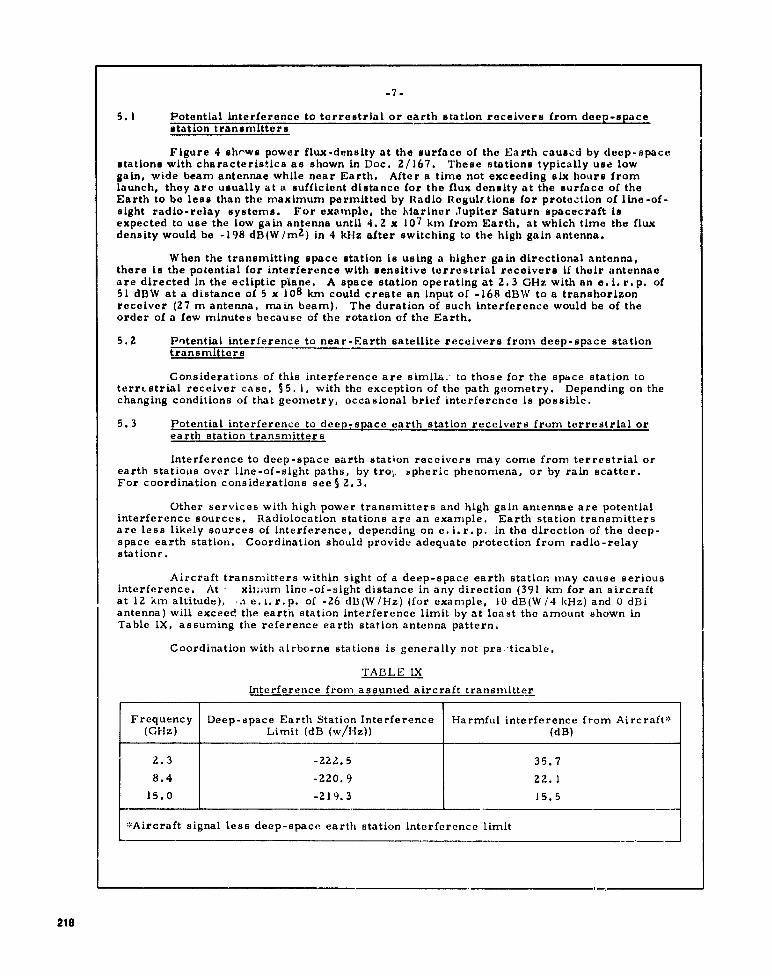
-7-
5. 1 Potential Interference to terrestrial or earth station receivers from deep-spacestation transmitters
Figure 4 shows power flux-density at the surface of the Earth caused by deep-spacestations with characteristics as shown in Doc. 2/167. These stations typically use lowgain, wide beam antennae while near Earth. After a time not exceeding six hours fromlaunch, they are usually at a sufficient distance for the flux density at the surface of theEarth to be less than the maximum permitted by Radio Regulations for protection of line-of-sight radio-relay systems. For example, the Mariner Jupiter Saturn spacecraft isexpected to use the low gain antenna until 4.2 x 10 7 km from Earth, at which time the fluxdensity would be -198 dB(W /m2 ) in 4 kHz after switching to the high gain antenna.
When the transmitting space station Is using a higher gain directional antenna,there is the potential for interference with sensitive terrestrial receivers if their antennaeare directed in the ecliptic plane. A space station operating at 2. 3 GHz with an e. I. r. p. of51 dBW at a distance of 5 x 10 8 km could create an input of -168 dBW to a transhorizonreceiver (27 m antenna, main beam). The duration of such interference would be of theorder of a few minutes because of the rotation of the Earth.
5.2 Potential interference to near-Earth satellite receivers from deep-space stationtransmitters
Considerations of this interference are simila.- to those for the space station toterrestrial receiver case, §5. 1, with the exception of the path geometry. Depending on thechanging conditions of that geometry, occasional brief interference is possible.
5.3 Potential interference to deep-space earth station receivers from terrestrial orearth station transmitters
Interference to deep-space earth station receivers may come from terrestrial orearth stations over line-of-sight paths, by tro t. Spheric phenomena, or by rain scatter.For coordination considerations see § 2. 3.
Other services with high power transmitters and high gain antennae are potentialinterference sources. Radiolocation stations are an example. Earth station transmittersare less likely sources of interference, depending on e, I. r. p. in the direction of the deep-space earth station. Coordination should provide adequate protection from radio-relaystations.
Aircraft transmitters within sight of a deep-space earth station may cause seriousinterference. At - xinjum line-of-sight distance in any direction (391 krn for an aircraftat 12 km altitude), a e. t. r. p, of -26 dB(W /Hz) (for example, 10 dB(W /4 kHz) and 0 dBiantenna) will exceed the earth station interference limit by at least the amount shown inTable IX, assuming the reference earth station antenna pattern.
Coordination with airborne stations is generally not pra,•ticable.
TABLE IX
Interference from assumed aircraft transmitter
Frequency(GI-1z)
Deep-space Earth Station InterferenceLimit (dB (w/Hz))
Harmful interference from Aircraft,(dB)
2.3 -222.5 35.7
8.4 -220.9 22.1
15.0 -219.3 15.5
*Aircraft signal less deep-space earth station interference limit
218

-8-
5.4 Potential interference to deep-space earth station receivers from near Earthsatellite transmitters
An analysis of the case for satellites in highly eccentric orbits may be found inReport AJ/2. It is concluded there that sharing is not feasible. This conclusion is alsovalid for satellites in circular and moderately eccentric orbits.
6. Discussion
Sharing with stations that are within line-of-sight (LOS) of deep-space earth stationsis not feasible. Stations within LOS will create excessive interference to receivers of deep-space earth stations, or will be exposed to excessive interference from transmitters ofthese stations. Aeronautical mobile stations and near-Earth satellites frequently comewithin LOS of deep-space earth stations.
Sharing of deep-space Earth-to-space bands with stations utilizing high averagee. I. r, p. is not feasible because of potential interference to stations in deep space. It iscurrently considered that stations with an e. I. r. p. that is more than 30 dB below theImplemented or planned e. 1. r. p, for space research earth stations do not pose a significantpr y 1 tem. From the data in 2/167, this means an average e. i. r. p, no gre y, r than 82 dBWat L And 7 GHz. The deep-space earth station e. I. r. p. for other frequencies is not nowknown.
7. Conclusion
Criteria and considerations presented in this Report lead to the followingconclusions:
7. 1 Sharing of Earth-to-space bands
Deep-space research cannot share Earth-to-space bands with.:
(a) receiving aeronautical mobile stations,
(b) receiving satellite stations, and
(c) transmitting terrestrial stations and earth stations utilizing high averagee. i. r, p. , for example, transmitting transhorizon stations, and transmitting fixed-satelliteearth stations.
When coordination is practicable, sharing is feasible with other stations of allservices. in some cases, coordination distane may be unacceptably great.
7.2 Sharing of space-to-Earth bands
Deep-space research cannot share apace-to-Earth bands with:
(a) transmitting aeronautical mobile stations, and
(b) transmitting satellite stations.
When coordination ib practicable, sharing is feasible with other stations of allservices. In some cases, coordination distance3 may be unacceptably great.
The matter of unacceptably long coordination distance requires further study.
219
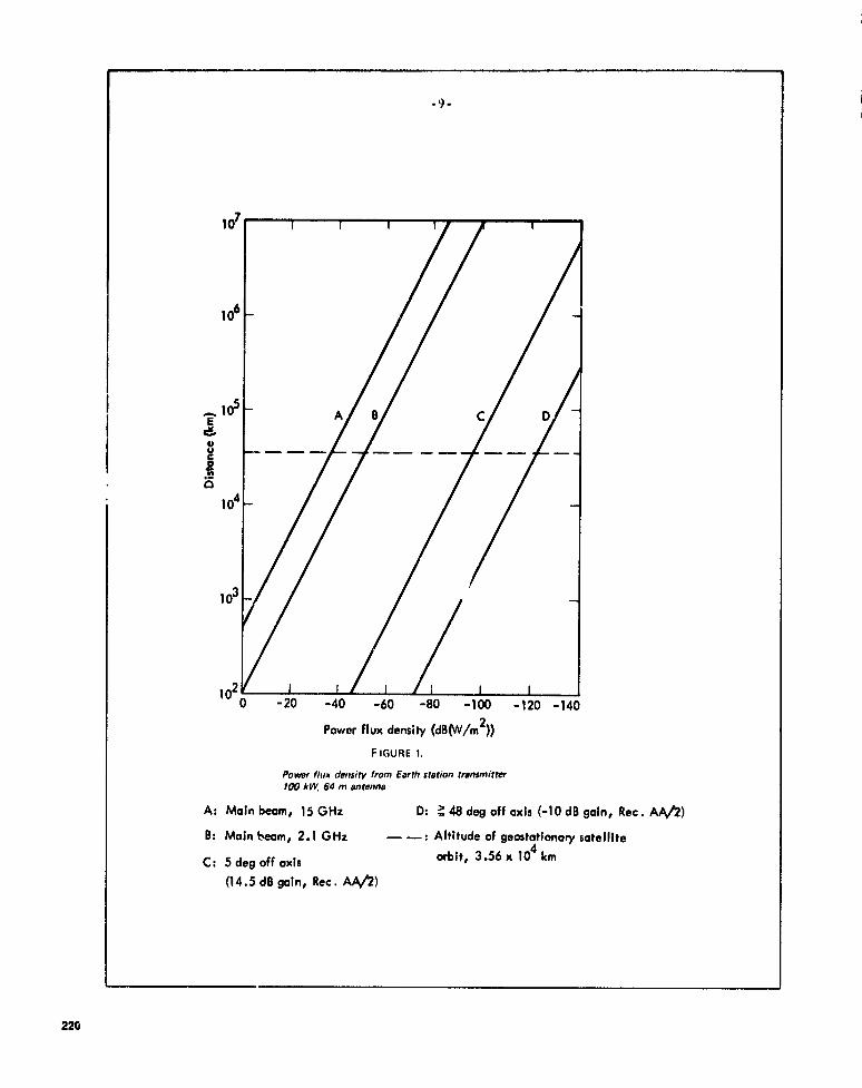
710
106
E 105
A B C D
veu
G104
103
102 0 -20 -40 -60 -80 -100 -120 -140
Power flux density (dB(W/m2))FIGURE 1.
Power flux density from Earth station transmitter100 kW, 64 m antenna
A: Main beam, 15 GHz D: a 48 deg off axis (-10 dB gain, Rec. AA/2)B: Main beam, 2.1 GHz — —: Altitude of geostationary satellite
C: 5 deg off axis orbit, 3.56 x 10⁴ km
(14.5 dB gain, Rec. AA/2)
-9-
220

b
Ln
rr
-40
.: -50N
mZ' -60
v>.r -70
O -80
x-40
O
-100EE
-110c^ o
0 10 20 30 40 50 60 70 60
Cumulative time at or above minimumpower flux density (minutes)
F GURE 2.
Duration of potendaf interference to geostationawsatellite intersecting beam axis from Earth stationwith 100 kW transmitter and 64 m antenna
2.1 GHz
--- . 15 GHz
NNJ

1010
106
109
105
-r-r
D
-
C
B
A
0 10 20 3
Space station urn c^n^u yu.n ^uu^f
FIGURE 3.Space station distance from terrestrial transnutter forinterference power equal to receiver noise power
A: 15 GHz relay transmitter, 55 dB(W/10 kHz); -168 dB(W/kHz) receiver noise powerB: 7.2 GHz relay transmitter, 55 dB(W/10 kHz); -170 dB(W/kHz) receiver noise powerC: 2.1 GHz relay transmitter, 55 dB(W/10 kHz); -171 dB(W/kHz) receiver noise powerD: 2.1 GHz transhorizon transmitter, 93 dB(W/10 kHz); -171 dB(W/kHz) receiver noise powerd: Space station range of 1 astronomical unit, 1.5 x 10 8 km
Evuc
vc00
wUS
d108
107
222
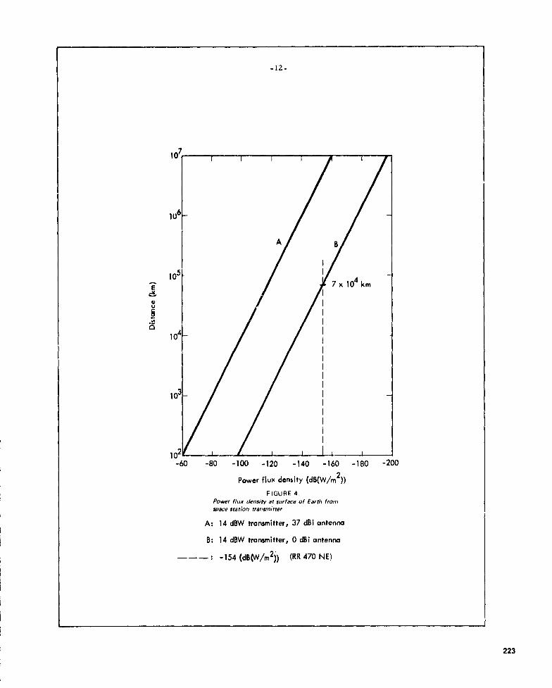
-12-
107
106
A B
105—
I
I104 km1 7x
Uu Ie IN
104
I^
I
I
j03—
I
I
I
I
I
I
I
102
I
I
-60 -80 -100 -120 -140 -160 -180 -200
Power flux density (dB(W/m2))
FIGURE 4.Power flux density at surface of Earth fromspace station !ransmirter
A: 14 dBW transmitter, 37 dBi antenna
B: 14 dBW transmitter, 0 dBi antenna
-- -154 (dB (W/m 2)) (RR 470 NE)
223

v L"^
DSN Progress Report 42-44 January and February 19713
N7g-2423'7
Development of a Unified Criterion forSolar Collector Selection
F. L. LansingDSN Engineering Section
To assist in making engineering or management decisions, tills article explores thepossibility of building a single selection criterion to distinguish between different solarcollector subsystems for a specific application or between different complete solar-powered systems. The development of two analogous criteria are discussed. Tire criteriacombines both performance and unit area costs, and presents the dollar per unit powerand the dollar per unit energy produced from a solar plant. Tvplcal values for currentfocusing and nonfocusing solar collectors were included to support tite discussion. Thefirst phase development shows that the criteria evaluation is in need of more dataabout the annual ' dynamic behavior of the collector subsystem only, under titetransient site-specific parameters such as solar flux, wind, and ambient temperature.
i. IntroductionIt is a fact that the last decade has witnessed a great deal
of research and development in nonfossil fuel energy sourcesto find a solution to the energy shortage problem. Manyindustrial organizations, academic institutes and researchlaboratories including the let Propulsion Laboratory, havestarted energy research and conservation programs Solarenergy as one of the nondepletable sources has been underthorough investigation, and the solar collector component, asan entity, has occupied a major part of that investigation.
The above competitive efforts blossomed many collectorconcepts. Some concepts are still on paper while others areahead in production phase. No bounds or standards are setto unify the parameters of module geometry, physicaldimensions, weight, operating temperatures, optical proper-
ties of coatings or glazing, insulation thicknesses, heat lossrates, etc. Consequently, large collections of information anddata regarding performance and cost of many "good" solarcollectors were established. The differences in cost andperformance are wide not only between collectors of differ-ent categories but also between collectors of the samecategory. Collector manufacturers enlarge this difference gapand support their own product selection rationale to obtaineither high performance using expensive high grade materialsor to sacrifice performance for a low cost product.
For a given application, the selection of the solar col-lector, whether it is a focusing or a nonfocusing type, affectsthe overall installation, operation and maintenance cost. Forengineering or management decisions, the question thateventually will rise is which collector possesses the "best"score? The comparative adjective "best" means in engineer-
224
ORIGINAL PAGE 1bOF 1,001t QUAUM

ing terms the one that not only scores highest in fulfilling itspurpose at the required operating conditions with the leastcost but also scores highest in reliability, durability, low risk,nonhazardous and low maintenance problems. Any costmethodology such as a life cycle cost analysis, a cost/benefitpayback period analysis, or a cash flow analysis, may beused to support the selection rationale.
In the present article, the development of a single col-lector criterion combining performance and unit cost isexplored to be used as a figure of merit. The otheroperational parameters of risk, maintenance, and reliabilityare not included for two reasons; ( 1) there is not enoughdata accumulated about collector failures, maintenance anddurability to judge a newly developed solar collector, and(2) reliability and maintenance figures of merit using theprobability theory are addressed elsewhere in detail andcould be added to the total selection of analysis once acost/performance criterion is established.
The main objectives of this study are set to (1) provide ameans to distinguish between different solar collectors orintegrated solar -powered systems for a given applicationcombining only performance and unit cost, (2) reduce oreliminate the need for costly site-specific experimental testsonce a good performance model is established at another sitewith different weather spectrum and (3) assist engineeringand/or management in making decisions in system evaluationand cost effectiveness.
11. Collectors for Electric Power GenerationIn comparing focusing collectors (such as parabolic
troughs, parabolic dishes, fresnel lenses, etc.) with nonfocus-ing types (such as flatplate collectors) for electric powergeneration, the points in favor and against each type are asfollows;
(1) Focusing collectors tend to have, in general, highercollection efficiency than nonfocusing types. This is causedby the reduction in heat losses as a result of small concentra-tion areas which is much less than the increase in heat lossescaused by high temperatures attained.
(2) Nonfocusing collectors have the ability to harness thediffuse radiation while focusing types do not have. Diffuseradiation can be as much as 20% of the total incident fluxon clear days. This ratio goes vr, on cloudy days. On theother hand, nonfocusing collectors are generally nontrackingand the radiation cosine losses due to their fixed obliqueorientation (cosine the angle of incidence) exceeds the gainof the extra diffuse part. The result is a less peak and
accumulated radiation intensity for clear days than trackingfocusing collectors. The situation is reversed on cloudy days.However, it appears that this extra diffuse part plays aninsignificant role in collection efficiency increase since non-focusing collectors have generally higher efficiency as statedin item (1).
(3) Although tracking in focusing collectors is essentialand adds an extra cost to the power plant, it is desirable inmaintaining a constant collector efficiency for longer periodsover the day. This is in contrast with nontracking nonfocus-ing types that possess an undesirable steep rate of efficiencydecrease with operating temperature.
The above points indicate that collectors with high perfor-mance are accompanied by high cost and vice versa. Theneed for a selection methodology then follows as an essentialtool for comparison of the various types.
The cost of a solar-electric power plant is greatly influ-enced by the overall conversion from solar-to-electric effi-ciency. If conversion is done via thermal power cycles, theefficiency is simply the product of collection efficiencytimes the power cycle thermal efficiency as shown in Fig. 1.
The efficiency trends shown in Fig.I for both thecollector and the power cycle are general for any type ofeach. The collection efficiency always decreases with increas-ing operating temperature due to higher thermal losses andcan reach zero when the incident radiation equals the lossesat point B. The power cycle efficiency, on the other hand,increases with the operating temperature and starts fromzero at ambient t, mperaturc, point A. The overall conversionefficiency will be zero at both points A and B and alwayspossesses a maximum value in between A and B. Theoptimum operating temperature corresponding to maximumoverall conversion efficiency should be the system designpoint.
Ill. Derivation of Maximum Solar/ElectricConversion Efficiency
The performance of solar collectors is generally the samewhether they are focusing or nonfocusing types. The -nstan-taneous collector efficiency (E^) can be expressed approxi-mately by the linear form
T- ToEC = a t - b t f (1)
226

where
/ ffi solar intensity per unit collector area
Toambient temperature
a tcollector constant representing its opticalefficiency
b t
collector constant representing its thermal losscoefficient
T = Plate (receiver) temperature of the collector
Equation (1) can be put in the compact linear form:
EC = a 2 - 11 T(2)
where a2 and b2 are collector constants given by
TOa2 = at + br
(-1)
It
hr
The constants a 2 , b 2 are considered collector "character-istic" constants to differentiate between shapes, geometry,optical and thermal properties for a given ambient tempera•ture and solar intensity.
On the other hand, the thermal efficiency of power cyclescall expressed ir, general as a fraction of the correspond-ing Carnot's cycle working between the same source/sinktemperature limits. This fraction is a function of manyconditions, such as type of cycle, type of working fluid,pressure and temperature ranges, etc.
The ratio (N) of real power cycle efficiency to Carnot'sworking between the same temperature Ifmits, ranges inpractice from 0.4 to 0.6 at full load. Accordingly, thethermal ,efficiency of a real power cycle working between ahot surface temperature T and an ambient temperature To isapproximated by
T
0)Ee = X ^I - (4)
The overall conversion froth solar to electric efficiency(Eo ) then follows as
Eo = EC X E
or by combining Eqs. (2) and (4)
TEo - A (a 2 - b 2 T) I - r /
(5)
The overall conversion efficiency from Eq. (5) can be zeroat two positions:
(1) Where the collector efficiency is zero at a maximumtemperature:
a
TB = n2. (point B on Fig. I )
2
(2) At a temperature TA = To , or when he engineeffi gy• -ency is zero at ambient temperature (point A onFig. 1).
Assuming that the parameters a 2 , b2 , and X areunchanged with the collector temperature, the )verall con-version efficiency will possess a maximum value Eo,max atthe optimum temperature T„pt given by differentiation as
T„p t = V°2 To b 2 (6)
T 2
T pr )
Equations (5) and (7) show that at the optimum operat-ing temperature
a
E,, _ ^ - Ep (R)
This means that if the value of (a 2 ) is equal to (X) theoptimum temperature (To pr ) will be file intersection pointI the engine efficiency and collector efficiency curves.The location of the optimum temperature will be lower thanthe intersection temperature or higher depending on whetherthe value of (a2 /X) is larger or smaller than I, respectively.
226

The optimum operating temperature for the combinedcollector-engine system as calculated from Eq. (6) is depen-dent on the slope (h 2 ) and ordinate intersection (a 2 ) of thecollector efficiency line. Smaller slopes and larger ordinateintersection produce higher overall conversion efficiency
E0.m.x and higher optimum temperature. This explains whyfocusing collectors are offering a superior performance com-pared to nonfocusing types.
IV. First Selection Criterion forSolar-Electric Plant ($/kWe)
From an engineering viewpoint, a solar-electric plantshould he combining good perfoi.nance (presented by themaximum overall conversion efficiency) and low cost tocompete with conventional fossil-fuel or nuclear powerplants. Before rating different collectors or different energyconversion systems, the following parameters and assump.tions will be fixed for all candidates under investigation:
(1) Operating temperature will be the optimum valuecorresponding to the maximum overall conversionefficiency.
(2) Site and location with its topography and geographyis the same to each candidate.
(3) Weather spectrum, ambient temperature, humidity,wind speed, and direction are the same to eachcandidate.
(4) Cloud cover, thickness, height, dispersion, rnd fre-quency of appearance are the same to each candidate.
(5) Clear day solar insolation spectrum is the same for allcandidates. Even though focusing and nonfocusingcollectors receive different proportions of direct,diffuse, and ground reflected parts, the conversionefficiency is assumed to be independent of theintensity of input energy. In other words, each col-lector will be scored and judged according to itsability to collect and transfer to the working fluid thesolar energy which was harnessed.
(6) Maintenance and operation costs (M&O) will beassumed in direct proportionality to the unit collectorcost ($/111 2 ). This means that expensive collectors willhave larger M&O costs than inexpensive ones. Theseannual costs will constitute a fixed percentage (oforder 10 for example) of the installation cost.
The collection surface area can be calculated from thesimple equation:
2 electric power output (kWe)collector area (m ) solar radiation intensity (kWt/nt 2 ) X
overall solar-electric conversionefficiency (EO,max l
(9)
The electric power output in the numerator and the solarradiation intensity in the denominator should be computedduring the same time Interval. The latter could be a 15-minpeak, a daily average, a monthly average, a seasonal averageor a yearly average. The overall solar-electric conversionefficiency is determined by using Eq. (7), with fixed solarradiation and ambient conditions.
Th.- installation cost in dollars of the whole solar powerplant including energy collection, conversion, storage, andtransport subsystems can be divided by the total collectionarea (in m 2 ) to yield a unit installation cost in ($/m 2 ). Theoperation and maintenance cost when added as a fixedpercentage of the installation cost will facilitate the compari-son, so that we need only to speak about the unit plantcost.
The total plant (or collector) cost per kW, output canthus be given by:
unit plant (or collector) cost
plant (or collector) $/kWe = ($/m2)solar radiation intensity (kWt/na g )X overall solar-electric conversionefficiency (E0,1nax)
(10)
Equation (10) applies to any solar-electric plant whetherit is an indirect thermal-electric conversion via power cyclesor a direct solar-electric conversion such as photovoltaiccells. Also, Eq. (10) can be used in comparing collectorsonly for solar-electric application by using the unit collectorcost $/tm 2 instead of the unit plant cost ( $/m2).
A common reference value of the solar radiation intensityis one "sun" defined as a peak intensity of I kWt/m 2 (0.1W/cm 2 or 317 Btu/11 ft 2 ) at solar noon. For trackingcollectors, the intensity of i kWt/m 2 is considered a suitableincident radiation reference. But for nontracking collectors, aradiation reference of 0.8 kWt/m 2 will be chosen as a
227

radiation reference to account for the cosine of the angle ofincidence losses. Under these radiation references, the cost ofany solar-electric plant (or collector) per electric kilowatt atthe bus bar can be given b y substituting in Equation (10).For solar-electric power plants with tracking solar collectors,
unit plant (or collector)
total plant (or collector cost) $/kWe . cost $/moverall conversion effi-ciency (Eo,m.x)
(I la)
For solar-electric power plants with nontracking solar collec-tors,
unit plant (or collector)
total plant (or collector) cost $/kWe = cost $/rn20.8 X overall conversionefficiency (Eo,maa)
(I lb)
Equations (I I a, b) present the first figure of merit($/kWe) which differentiates between the different solar-electric conversion systems combining both performance andcost. Other figures of merit representing maintainability, risk,durability, etc., can be added to complete the selectioncriteria.
Table I lists typical results for some current solar collec-tors. The instantaneous efficiency curves are plotted asshown in Fig. 2 versus the average collector temperature. Theheat engine efficiency working at 50% of Carrot's betweenthe collector temperature and ambient temperature 25°C(77°F) is also plotted for reference. Some cost and effi-ciency data were abstracted from Refs. I through 12.
Equations (6) and (7) are used to calculate the optimumoperating temperature and the maximum overall conversionefficiency, respectively. The unit collector cost ($/m2)figures were either abstracted from manufacturer data orestimated from past experience. Equations ( I I a, b) are usedto estimate the $/kWe figures as given in Table I. Themaximum overall conversion efficiencies were in good agree-ment with some of the values reported in Refs. 13 and 14using other derivations.
It is apparent from Table 1 that focusing collectors withtheir high temperature capability, in spite of their high cost,are favored for solar-electric conversion. However, the rate of
228
decreasing costs by mass production in focusing and non-focusing types can change the selection procedure. Table 2for example, shows how the competition between solarcollectors can be tough. The three hypothetical solar collec.tors presented in Table 2 have different optimum perfor-mance figures as presented by 3%, 87o, and 16% conversionefficiency and different unit cost as given by $60, $200, andS400/0. According to Eq. (11), the collector cost alone perWe output is the same for all of them and equals$2500/kWe which appears to make the selection process notdecisive. The first collector could be a typical flat platecollector as evidenced in Table 1. Also, the second collectorcould be a low performance parabolic trough, and the thirdcollector could be a paraboloid, dish or a heliostat powertower collector. Furthermore, if the rest of t,te subsystemssuch as energy transport, conversion, and storage subsystems,excluding the collector subsystem, cost the same whenproducing I Me, then the choice will still be narroweddown to that collector which requires the least land area forthe given output. Table 2 shows that collection areas rangefrom 6 to 42 m 2 /kWe for the above cases depending on theoverall conversion efficiency as given in Eq. (9). This collec-tion area should further allow for shadowing effects, modulespacing, etc., which means larger land areas and moreinstallation cost. For these nondecisive cases, knowledge ofcollector performance over longer periods of time is veryimportant, which leads to the second analogous criterion inthe next section.
V. Second Selection Criterion forSoler-Electric Plenty ($/kWhe)
The unit plant (or collector) cost in $/kWe derived in thelast section cannot stand alone as the sole criterion forcomparing different types of collectors. The "$/kWe" figurehas been derived based on "instantaneous" collector effi-ciencies measured at noon time with a fixed value of solarinsolation and assuming a quasi-steady-state operation(I kWt /m 2 for tracking collectors or 0.8 kWt/n1 2 for non-tracking types). In practice, solar collectors do not actuallyoperate at their steady-state conditions since they are subjectto many site-specific time varying; variables such as solarflux, ambient temperatures and wind speed.
A collector response time, defined as the time taken toreach 9910 of its steady-state temperature under a stepchange of the solar flux, is known to vary from a fewminutes to about one hour according to the collectorthermal capacitance. It appears, therefore, that a criterionbased on a performance measure integrated (or accumulated)over a day, a month, or a year period would be moresuitable in comparing different solar-electric power plants
ORPAGE Its
^G^AL(
GUAL^1F poo?'

encompassing these transient conditions. The unit energycost (S/kWhe) produced by a solar-electric plant with perfor-mance integrated over one year could act as a secondselection criterion to represent the effects of the dynamicand site-specific performance. Th y derivation of this criterioncan be simplified as follows: C S A c XCc XR (14)
fraction of the collector subsystem cost. Also, the annualmaintenance and operation cost will be assumed in propor-tion to the total installation cost. Consequently, Eq. (13)could be rewritten as
Let the annual electrical energy generated from a solar•electric power p!.tnt (W*) in kWhe be given by
W* n 10 XA C XE, XE,,* XE,,* XE,*r 02a)
or
W* - IXA C X.Eo (12b)
where
1* - accumulated annual solar flux, kWht/year
A C = collectors area, m2
El = accumulated annual collection efficiency
Ee* = annual engine efficiency
Es = annual storage subsystem efficiency
ET = annual energy transport subsystem efficiency
Eo = annual overall solar-electric efficiency
The annual cost (C) in dollars could be calculated usingthe cost recovery factor (CRF) of the borrowed money in alifetime mortgage plan as
collector subsystem cost+ storage subsystem cost
annual cost (C) _ + energy conservation subsystem cost+ energy transport subsystem cost
X [cost recovery factor (CRn]
+ annual maintenance and operationcost
(13)
In most applications, the energy storage, transport, andconversion subsystems cost will be assumed to be a fixed
where Cc is the collector cost per unit area (S/m 2 ), and R isthe ratio of the total annual cost to the total collector cost.For example, if the collectors lifetime is taken as 20 yearsand the interest rate on the borrowed money is 8%. the(CRF) will be 0.10185 S/yr With approximately a 4:1 ratiobetween total installation to collector cost, the ratio R is
found to be around 0.4.
The cost per unit electrical energy output then follows bycombining Eqs. (12b) and (14) as
C CCW*
cost/kWhe = =1*
• E:
(I 5)0
For example, if a paraboloid solar collector is built with450 S/m 2 , a ratio of R of 0.4, an annual overall solar-electric conversion of 0. 18, and an accumulated annualinsolation of 3126 kWht/m 2 (a daily average direct normalflux of 8.7576 kWht/m 2 such as that measured at Goldstonearea, California) the cost per kWhe produced would beapproximately 0.31 dollars.
The cost/kWhe viiterion expressed mathematically in Eq.(15) indicates that in order to generate low cost electricalenergy, the parameters, Cc. R, P and Eo should be inharmony with each other and not separately optimized. Forinstance, if a fiat plate collector, having a unit cost of 60$/m 2 , an annual conversion efficiency of 0.03 and an annualsolar flux of 2604 kWht/m 2 , is compared with the aboveparaboloid dish example with the same ratio of R of 0.4, thecost of energy produced would be 0.307 dollars/kWhe whichis approximately the same for both types. The first collector(paraboloid dish) has a high unit cost (C,), receives highsolar flux as a result of tracking, and has a high conversionefficiency because of its high operation temperature. Thesecond collector is completely opposite to the first, but bothproduce energy with the same cost. The final selection inthis case should be guided by other factors such as durabil-ity, maintainability, land areas, visibility etc.
The second criterion shows clearly the important need ofaccurate site-specific transient analyses to predict the annualconversion efficiency (Eo) of different solar-electricsystemsto support the first criterion. which is not site-specific.
229

VI. Solar-Cooling ApplicationTo use the solar energy as a driving force for cooling
devices, several well-known concepts can be coupled with aheat source, Shown fit 3 are the coefficient of perfor-mance trends versus the collection fluid temperature leavingthe collector subsystem for sonic of the above concepts,Superimposed on Fig, 3 is the general behavior of thecollector efficiency. The overall coefficient of performance(OCOI') is defined as the ratio between the refrigerationeffect (Q,) and the incident solar flux (Q r ) as illustrated inFig. 3. T5us
For tracking solar collectors (intensity - I M/nt 2 ):
total plant unit plant (or collector) cost $ /m2(collector) = 3.516 Xcost $/Ton overall coefficient of performance
(OCOP)ui o z fromsolar-refrigeration effect
(I8a)
For nontracking solar collectors (at intensity of 0.8 Mt /nO )
total plantunit lane (or collector) cost $/10
(collector) = 4.4 X overall ateflicient of perfonnartceQ^ Q^ Q= cost $/Ton
OCOP a Q3 = 03 X Q2 (16) (OCOP).., frontQ IQz Qt solar-refrigeration effect
or(I8h)
collector cooling[OCOP] subsystem X subsystem (17)
efficiency COP
The overall system performance possesses always a maxi-mum value at an optimum temperature in between theambient temperature (A) (where the coefficient of perfor-mance of the cooling subsystem is zero) and the equilibriumcollector temperature (B) (where the collector thermal lossesare equal to the incident solar flux). The point of ntaxintuntOCOP should be the selected design point, and is usuallydetermined by curve plotting instead of analyticalexpressions.
Similar to the discussion presented in Section IV, the unitpower cost ($/kWe) for solar-electric application will bereplaced here by the unit power cost ($/Tons of refrigera-tion' ) for solar-cooling devices. The overall solar-electricconversion efficiency (f'o , max) will also be replaced by theoverall-solar-cooling effect coefficient of performanceWON ax . All other parameters bear the same meaning.
The first criterion, presented in Equations (Ila, b) forsolar-electric conversion, could be rewritten then for solar-driven refrigeration devices as follows:
'One ton of refrigera:ion = 12000 Btu/h = 3.516 M cooling energy
230
Also, for the second criterion, the cost per unit "cooling"energy or $/(Ton-h) could be derived by the saute procedureused for solar-electric plants. Analogous to Eq. 15, the($/Ton-h) could be written as:
3.510- Rcost
11)
l* • (OCO/')*
where MOP)* is the accumulated annual overall coefficientof performance (from solar flux-to-refrigeration effect). Allthe other parameters heal same meaning as before.Again, the transient response to the fluctuating solar flux,
ambient conditions and wind speed, etc., are very necessaryin order to estimate the annual performance before com.paring different refrigeration schemes.
VII. Soler-Heating ApplicationFor this particular application, the first criterion does not
apply and only the second one does. The estimated unit costof thermal energy collected ($/kWht) is the key numberneeded for comparison with other conventional heatingdevices such as fuel-fired boilers, electric heaters, or heatpumps. Analogous to Eq. (15), the ( $(kWht) is written forsolar heating as
C -Runit energy cost $/kwht = —` (20)
1* E*
where 1s'fr is the combined annual efficiency of the collectorsand storage subsystems. All other parameters bear the saute
CIRIGINAL PAGE: 1D
op POOR QUALITY

meaning as used before. Only in solar heating applications,the value of the operating fluid temperature has to bespecified in adv ace before calculating EN. For example, ifthe solar heating application is for space heating Cher. the EHwould be estimated with the candidate collectors produc'nga uniform temperature of 49°C (120°F), which is enough forthis application. For domestic hot water use, a temperatureranging from 60 to 82°C (140 to 180°F) is adequate, andshall be used for estimating EH*. This means that theevaluation of EO is assumed to be done at a single value ofcollector temperature, for all competing collectors, irrespec-tive of the possible ranges of higher temperature beyond thisvalue that each collector can reach. Therefore, each collectorwill be judged on how much annual energy was collectedfrom the sun and transferred to the end point at a prespeci-f►ed heating temperature. Once more, for heating application,the collectors transient behavior and their sensitivity totime-varying input data, is of great value to any comparisonprocess.
VIII. Summary
The following points summarize the present study:
(1) To make a good engineering or management decision
as to which collector or solar-conversion deviceshould be used in a given solar application, twoanalogous selection criteria are presented. The firstcriterion gives the unit cost per unit power produced,based on instantaneous solar radiation or noon-timeflux. The ($/kWe) for solar-electric application andthe ($/Ton) for solar-refrigeration devices, are twoexamples of the first criterion. The second criteriongives the unit cost per unit energy accumulated (orintegrated) over a year period and taking into consid-eration the fluctuating nature of the solar flux,ambient temperature, wind speed and the thermalcapacitance of the collector itself. The ($/kWhe) forsolar-electric conversion, the ($/Ton • h) for solar-refrigeration conversion and the ($/kWht) for solar-heating are examples of the second criterion.
(2) The first criterion was tested for solar-thermal-electricconversion and for 13 types of available collectors(Table 1). The ($/kWe) figure was found lowestamong tracking and focusing collectors and highestamong flat-plate, nonfocusing, nontracking collectors.However, the need for transient performance data forthe second criterion ($/kWhe) is found very essentialbefore a final selection process can be made.
231
References
I. Simon, F., Solar Collector Performance Evaluation with the NASA-Lewis Solar-Simulator -Results for an All-(;lass-Evacuated Tubular Selectivel y-Coated Collectorwith a Diffuse Reflector, NASA TMX-71695. NASA Lewis Research Center,Cleveland, Ohio. April I, 1975.
2. Ari Rabl, Optical and Thermal Properties of Compound Parabolic Concentrators,Argonne National Lab, Argonne, Illinois, February 1975.
3. Performance Stuc/v of the Compound Parabolic Concentrator Solar Collector,report prepared by Environmental Consulting Services Inc., Boulder, Colorado, foithe Argonne National Laboratory, September 1974.
4. Corning 7bbular Evacuated Collector, Conning Glass Works, Lighting ProductsDivision, Corning, New York, January 1975.
5. Simon, F., Rat-Plate Solar-Collector Performance Evaluation with a Solar Simula-tor as a Basis for Collector Selection and rerfimnance 11redktionn, NASA TMX-71793, NASA Lewis Research Center, Cleveland, Ohio.
6. Kleinkauf, W., Kohne, R., Lindner, F. and Simon, M., "A Solar Power Plant in the10 KWe Range with Focusing Collectors", International Aerospace Abstracts byTechnical Information Service of AIAA, paper No. A76 .45995, American Instituteof Astronautics and Aeronautics, New York, New York, March 1976.
7. Ramsey, J. W., Sparrow, E. M., and Eckert, E. R. G., "Solar Thermal ElectricPower Generation Lying a System of Distrihuted Parabolic Trough Collectors", inInternational Aerospace Abstracts issued by Technical Information Service AIAA,paper No. A75 .47511, American Institute of Astronautics and Aeronautics, NewYork, New York, August 1975.
8. Solar Energy Program Semiannual Review Report, Sandia Laboratories, Albuquer-que, New Mexico, July 1976.
9. Northrop Collector, Northrup Incorporated, 302 Nichols Drive, Hutchins, Texas,1975.
10.Shimada, K., Swerdling, M., Terrestrial Solar Thermonic L'nergv ConversionSvsterns Concept, JPL Technical Memorandum 33-744, Jet Propulsion Laboratory,Pasadena, California, November 1975.
11. Lansing, F., and Dorman, J., "High Efficiency Solar Concentrator," Deep SpaceNetwork Progress Report 42-35, Jet Propulsion Laboratory, Pasadena, California.October 1976, pp. 99--109.
12.Anderson, D. E., and Stickley, R. A., "A Line Focus Segmented Mirror Concen-trator", SPIE Vol. 85 Optics in Solar E nergv Utilization 11, 1976 pp. 121-- 127.
13.Athey, R. E., "Evaluation of the Flat Plate Solar Collector System for ElectricPower Generation", Solar Energy, Vol. 18, 1976, pp 143-147.
14.Barber, R. E., "Solar Powered Organic Rankine Cycle Engines — Characteristicsand Cost", IIill Intersociety Energy Conversion Engineering Conference, IECEC,Vol. 2, 1976, pp. 1151--1156, Society of Automotive Engineers, Nev. , York.
232
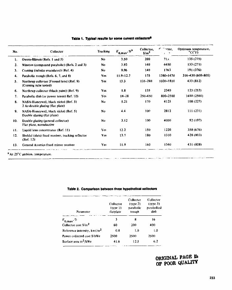
Table 1. Typical results for some current collectors
No. Collector Tracking %aO,max
Collect r,$/rrt
r ^1Pr, Optimum temperature,
1. Owens-Illinois (Refs. i and 5) No 3.50 200 71.). 135 (275)
2. Winston (compound parabolic) (Refs. 2 and 3) No 3.93 140 4450 133 (271)
3. Croning (tubular evaculated) (Ref. 4) No 9.96 140 1763 191 (376)
4. Parabolic trough (Ref's. 6, 7, and 8) Yes 11.9-12.7 175 1380-1470 316430 (600-805)
S. Northrup collecior (Fresnel lens) (Ref. 9) Yes 13.3 135-240 1020-1810 433 (812)(Corning tube tested)
6. Northrup collector (black paint) (Ref. 9) Yes 5.8 135 2340 123 (253)
7. Parabolic dish (or power tower) Ref. 10) Yes 18-28 250450 800-2500 1400 (2560)
8. NASA-Honeywell, black nickel (Ref. 5) No 5.21 170 4125 108 (227)2 Ar-double glazing (flat plate)
9. NASA-Honeywell, black nickel (Ref. 5) No 4.4 100 2812 111 (231)Double glazing (flat plate)
10. Double glazing (general collector) No 3.12 100 4000 92(197)Flat plate, nonselective
i I. Liquid fens concentrator (Ref. i l) Yes 12.2 ISO 1220 358 (676)
12. Sheldal (slats) fixed receiver, tracking reflector Yes 13.7 ISO 1310 428 (803)(Ref. 12)
13. General Atomics fixed mirror receiver Yes 11.9 160 1340 431 (808)
a At 25°C antbien, temperature.
Table 2. Comparison between three hypothetical collectors
Collector CollectorCollector (type 2) (type 3)(type 1) parabolic paraboliod
Parameter tlatplate trough dish
6 0,max' % 3 8 16Collector cost $/m 2 60 200 400Reference intensity, kwt/m 2 0.8 1.0 1.0Power collected cost $/kWe 2500 2500 2500Surface area m 2 /kWe 41.6 12.5 6.2
ORIGINAL PAGE IbOF POOR QUALITY
233

THFRMALfFFICIfNCY
ANY ENGINE(PRESENTED AS AFRACTION OFCAN NOT'S)
--AMBIENT ANY COLLECTORTEMPERATURE (APPROXIMATED
AS A ST. LINE)
MAX OVERALL / ^.+ a te` COMBINEDCONVERSIONEFFICIENCY
- " SYSTEMDESIGNPOINT
q0 A COLLECTOR TEMPERATURE
/ SOLAR _
\ . .% ENERGY ""'^" THERMAL
COLLFCTOR FEGINE ELECTRIC
( EFFICIENCYCONVERSIONFFICENCYONVERSION
fEFFICIENCY ( EFFIC ENCY E
J
Fig. t. Optimization of solar thermal -olectric convention
,,.—CORNING (EVAC TABULAR) *AMBIENT TEMP 25•C (77°F)
.—NASA-;:CNFYWELL 2AR FLAT PLATE *SOLAR INSOLATION 0.79 kW m2(250 Blu h tt2)
I GENERAL-ELECTRICy DOUBLE GLAZING, FLAT PLATE
WINSTON (COMPOUND PARABOLIC)OWENSALLINOISE
^— NASA -HONEYWELL (5)
1.0
0.9
0.8
0.7
w
v: 0.6Ww
0.5
ux 0.4H
0.3
0.2
0.1
0
NORTHRUP (1)
/---PARABOLIC (3)
LIQUIDLENS
PARABOLIC (2)\— PARABOLIC (1)
TYPICALHEATENGINE(50% OF CARNOTS)
1500 1 600 700 800 900 1000 1100 1200 1300
COLLECTOR TEMPERATURE, °R ( • F # 460)l 1 1 1 l I
0 25 100 200 300 400
COLLECTOR TEMPERATURE, °C
Fig. 2. Performance curves for some current solar collectors
234
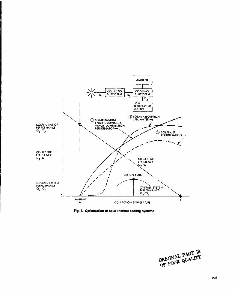
I AMBIENT I
\I / COLLECTOR COOLINGSUBSYSTEM SUBSYSTEM/0 QI Q2
Q3
LO WTEMPERATURESOURCE
02 SOLAR ABSORPTIONIQ SOLAR E (LiBr/WAT
COEFFICIENT OF ENGINEE
DRIVI NG AVAPOR-COMPRESSION
PERFORMANCE REFRIGERATOR—•^Q ,Q3 2 0 SOLAR-JETREFRIGERATION
COLLECTOREFFICIENCYQ2 Q I f COLLECTOR
EFFICIENCYJG/ Q2/QI
/ DESIGN POINT
OVERALL SYSTEMPERFORMANCEQ3. QI
/ OVERALL SYSTEM/ / PERFORMANCE
O ^_ , Q3 /Q I
AMBIENT BA COLLECTION TEMPERATURE
Fig. 3. Optimization of solar-thermal cooling systems
AL PAGE 1b
0 LIGT 4 GUp•L1'1KO
235

DSN Progreaa Report 42-44
January and February 1978
Implementation of Automated Fault Isolation TestPrograms for Maximum Likelihood Convolutional
Decoder (MCD) MaintenanceM. E. Alberda
DSN Data Systems Section
This article describes the automated fault isolation test programs that have beendeveloped to support rapid tum-around factory (or depot) level maintenance of theMaximum Likelihood Convolutional Decoder (MCD). Functional requirements anddetailed design characteristics are described, along with a summary of the evaluationand testing completed so far.
I. IntroductionTest programs, run on a computerized Logic Card tester,
have been developed to support rapid turn-around factory(or depot) level maintenance for the MCD, which is cur-rently being installed throughout the DSN as a part of theTelemetry Subsystem. The' MCD requirements and designcharacteristics are described in a previous DSN Report(Ref. 1).
These programs were entirely developed based on the useof existing design test equipment and support software inorder to realize maximum economy with minimum develop-ment time, and at the same tame achieve excellent overallfault isolation capability and extensive computer generateddocumentation.
One program for each of the two MCD plug-in circuitcards has been developed. In size and complexity, the MCDInterface Board contains 59 Integrated Circuits (IC's) widethe Decoder Board contains 92 IC's.
These programs were developed specifically to support aF.aranteed maximum repair time of 30 calendar days, at the
repair facility, regardless of the nature or extent of thefailure (e;_epting, of course, unforeseen catastrophic caseswhere a whole circuit board would have to be replaced).Also, a condition was added that if the expected repaireffort, to be accomplished on a "time-and-material" costbasis, exceeded a predetermined threshold level, then the 30day maximum period was to begin after .receiving formalauthorization to proceed with the repair effort from JPL.
In acceptance testing, the Interface Board program cor-rectly identified 92% of the random customer selected faultsmanually inserted, while the Decoder Board program cor-rectly identified 98% of the faults inserted (50 faults perboard).
II. Specific Functional RequirementsThe definition of the required performance characteristics
for these programs is contained in the JPL TechnicalRequirements Document (Ref. 2).
The salient functional requirements, and the factors usedin their selection, are discussed briefly below.
236

A. Logic TesterThe Mirco Model 530 Tester was selected as the test unit
to be used for the following reasons:
(1) Readily available (a standard catalog item).
(2) Reasonable cost.
(3) Rapid processing speed (200 KHz. Instruction rate).
(4) Ease of Maintenance and Operation.
(5) Availability of powerful support software, i.e., theFLASH (Fault Location And Simulation Hybrid)Simulator (Ref. 6), which offers greatly reduced pro-gramming time, improved testing comprehensiveness,and also provides computer generated programdocumentation.
B. Fault Isolation CapabilityEach test program was required to be capable of identi-
fying a circuit fault to within one IC (as a design goal) butin any event to within a group of not more than ten IC's, asan upper limit design goal.
The TRD also specified that, of the total number offaults simulated by FLASH (which includes shorts, opens,grounds, etc. for all circuit nodes on the board) at least 85%shall be correctly identified by each program.
Furthermore, all undetected (or incorrectly identified)faults were required to be isolatable using the availablemanual procedures called "Scope Trace" and/or "Time-Nodal-Test" transition counting.
C. Program Acceptance Test Procedure (PATP)A specific PATP was required for each program. These
procedures each contained a requirement that fifty (50)random customer selected faults (grounds) be inserted oneach known good board, one fault at a time, and the testprograms should correctly identify at least 85% of theseknown faults.
III. Design ApproachThe basic approach used for this development effort was
selected based on an awareness of commonly used digitaltest techniques and test equipment, including various typesof test stimuli generation (psuedo-random, manually gener.ated, etc.).
The utilization of FLASH was selected because of itsability to methodically and rapidly simulate all possible
faults, of all types, by use of its software modeling capabil-ity. This was considered to be far more complete, andeconomical, than other approaches involving more conven-tional manual techniques, of test stimuli generation andhardware testing (destructive and non-destructive).
Additionally, FLASH offered the advantages of reduceddevelopment time and effort, since it was fully developedand checked out, and had been successfully used on severalprevious test program developments of a similar type.FLASH offered the most complete and effective approachknown, it was felt, because in addition to the primaryautomated mode of operation, it provided the data necessaryfor the two manual back-up modes called SCOPE TRACEand Time-Nodal-Test (TNT) Counts. By use of these back-upmodes, fully non-ambiguous fault isolation can be achieved,involving minimal time, effort and operator skill.
IV. Design DescriptionA brief description of the Tester hardware and of the test
software development, documentation and utilization is pre-sented below. Detailed descriptions covering these subjectsare provided in Refs. 3 through 10. The Tester and the testsoftware are designed to evaluate circuit beards which con-tain all digital (i.e. 2-level) circuit devices.
A. Tester DescriptionThe Tester used is the Mirco Model 530. This unit is
portable, totally self-contained, includes all operator controlsand displays on its top surface, and the boards to be testedmount directly to it via customized Interface Adaptor con-nection units, one for each of the two board types to betested and one to be used with the Tester itself in itsSelf-Test mode.
The physical characteristics for this unit are listed below.
(1) Input Power — 270 Watts (115 V.A.C., 60 Hz)
(2) Size — 22.86 cm high58.42 cm wide40.64 cm deep
(3) Weight — 24.9 kilograms
(4) Operating Environment — 10°C (50°F) to 49°C(1200 F), with 10 — 90% relative humidity.
(5) Operator Panel — See Figure 1 (for more detail, seeRef. 8).
The Tester contains a microprogrammed test processor toexecute the stored test program and to monitor and evaluatethe test results. The processor instructions are implemented
237
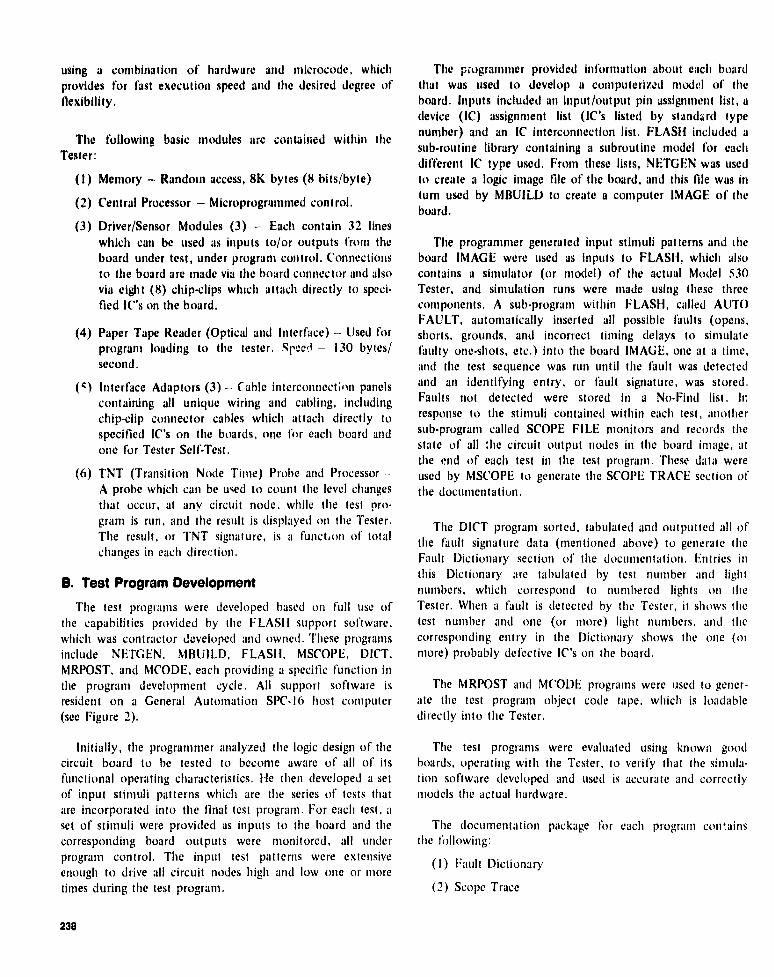
using a combination of hardware and microcode, whichprovides for fast execution speed and the desired degree offlexibility.
The following basic modules arc contained within theTester:
(1) Memory — Random access, 8K bytes (8 bits/byte)
(2) Central Processor — Microprogrammed control.
(3) Driver/Sensor Modules (3) - Each contain 32 lineswhich can be used as inputs to/or outputs frontboard under test, under program control. Connectionsto the board are made via the board connector and alsovia eight (8) chip-clips which attach directly to speci-fied IC's oil board.
(4) Paper Tape Reader (Optical and Interface) — Used forprogram loading to the tester. geed — 130 bytes/second.
( S ) Interface Adaptors (3) — Cable interconnection panelscontaining all unique wiring and cabling, includingchip-clip connector cables which attach directly tospecified IC's on the boards, one for each board andone for Tester Self-Test.
(G) TNT (Transition Node Time) Probe and Processor —A probe which can be used to count the level changesthat occur, at anv circuit node, while the test p ro-gram is run, and the result is displayed oil Tester.The result, or TNT signature, is a function of totalchanges in each direction.
B. Test Program DevelopmentThe test programs were developed based oil use of
the capabilities provided by the FLASH support software,which was contractor developed and owned. These programsinclude NETGEN, MBUILD, FLASH, MSCOPE, DICT,MRPOST, and MCODE, cacti providing a specific function inthe program development cycle. Ali support software isresident on a General Automation SPC-16 host computer(see Figure 2).
Initially, the programmer analyzed the logic design of thecircuit board to be tested to become aware of all of itsfunctional operating characteristics. He then developed a setof input stimuli patterns which are the series of tests thatare incorporated into the final test program. For each test, aset of stimuli were provided as inputs to the board and thecorresponding board outputs were monitored, all underprogram control. The input test patterns were extensiveenough to drive all circuit nodes high and low one or moretimes during the test program.
The p;ogratnmer provided information about each boardthat was used to develop a computerized model of theboard. Inputs included an input/output pin assignment list, adevice (IC) assignment list (IC's listed by standard typenumber) and an IC interconnection list. FLASH included asubroutine library containing a subroutine model for eachdifferent IC type used. Front lists, NETGEN was usedto create a logic image file of the board, and this rile was inturn used by MBUILD to create a computer IMAGE of theboard.
The programmer generated input stimuli patterns and theboard IMAGE were used as inputs to FLASH, which alsocontains a simulator (or model) of the actual Model 530Tester, and simulation runs were made using these threecomponents. A sub-program within FLASH, called AUTOFAULT, automatically inserted all possible faults (opens,shorts, grounds, and incorrect timing delays to simulatefaulty one-shots, etc.) into the board IMAGE, one at a time,and the test sequence was run until the fault was detectedand all entry, or fault signature, was stored.Faults not detected were stored in a No-Find list. Ir.response to the stimuli contained within each test, anothersub-program called SCOPE FILE monitors and records thestate of all ;he circuit output nodes in the board image, atthe end of cacti test in the test program. These data wereused by MSCOPE to generate the SCOPE TRACE section ofthe dOCUrrrentatiun.
The DICT program sorted, tabulated and outputted all ofthe fault signature data (mentioned above) to generate theFault Dictionary section of' the documentation. Entries inthis Dictionary are tabulated by test number and lightnumbers, which correspond to numbered lights oilTester. When a fault is detected by the Tester, it shows thetest number and one (or more) light numbers, and thecorresponding entry in the Dictionary shows the one (ormore) probably defective IC's oil board.
The MRPOST and MCODE programs were used to gener-ate the test program object code tape. which is loadabledirectly into the Tester.
The test programs were evaluated using known goodboards, operating with the Tester, to verify that the simula-tion software developed and used is accurate and correctlymodels the actual hardware.
The documentation package for each program containsthe following:
(1) Fault Dictionary
(2) Scope Trace
238

(3) No-Find List
(4) Source and Object Programs Listings
(5) Interface Adaptor Wire Ust
(6) TNT Counts — for all circuit nodes.
(7) Statistics Summary Sheet (See Figures 3 and 4)
The Statistics sheet shows the comprehensiveness, orpercentage of total faults found, and also the fault isolationachieved, or percentage of isolation to one, vs. two or more,IC's. As indicated, 93% comprehensiveness was achieved forthe MCD Interface board and 94.9% for the Decoder board.Thus most faults (93 — 95%) will he detected oil firstrun of the test program. Run time is less than 0.2 second foreach program. For resolving undetected faults, or for improv-ing fault isolation (if needed), two approaches are available.One is to evaluate each fault in the No-Find list, and bysearching the Scope-Trace table, find a test where the subjectcircuit node should have .hanged state, then monitor thisnode with a separate oscilloscope and probe to determinewhether or not the node is changing as shown by the ScopeTrace. The other approach is to use the TNT probe, with theTester, to count transitions at various suspect circuit nodes,based on general knowledge of the boars operation and onthe known symptoms of the malfunctions. Correct countshave been tabulated for all circuit nodes for each board.Many nodes can be checked in a short time because totalrun time is so short. Each repaired MCD will be re-testedusing the MCD Acceptance Test Procedure (Ref. 1) to verifyoperational readiness.
V. Testing and EvaluationThe testing done so far consists of the Program Accept-
ance Tests wluch were completed at the end of the develop-ment cycle. As indicated above, fifty random faults(grounds) per board were selected by the customer andinserted, one at a time, on each board and the appropriate
test program was run on the Tester, after the board hadbeen mounted to the Tester via its Interface Adaptor.
(1) Interface Board46 of 50 faults were detected and correctly identi•tied, giving an accuracy of 92%n. Of the 4 remainingfaults, 3 were detected as test failures by the pro-gram, but the program did not identify the actuallocation of the faults by IC number and pillThe program failed to detect the other fault andshowed a PASS condition.
(2) Decoder Board49 of 50 faults were detected and correctly identi-fied. giving an accuracy of 98%. The oue remainingfault was detected by the program, but not correctlyidentified to the actual location.
The back-up fault r tctection and isolation proceduresusing Scope Trace and TNT counting were not evaluated atthe time of the Accepta ► ,ce tests, but will be exercised andevaluated in the near furtre 'These procedures will be usedto verify the fault location, as indicated by the FaultDictionary, following a normal run of the test program. Inthis way faults will be positively identified before any IC'sare replaced.
Through Dec. 1977, there have been two MCD unitsrepaired at the factory, us ing these programs, and their use wasentirely satisfactory. Additional performance data will beaccumulated as these p rograms continue to be used for MCDrepairs, in supporting the 33 MCD units which have beendelivered to the USN, since the last delivery from the factoryin April 1976.
VI. ConclusionThe entire development of these programs proceeded as
initially planned, on schedule and within budget, and thefinal performance quality exceeded the fixed, and the designgoal, requirements specified in the TRD.
239

References
1. Alberda, M. E., "Implementation of a Maximum Likelihood Convolutional De-coder in the DSN", in The Deep Space Network Progress Report 42 .37, pp.176. 183, Jet Propulsion Laboratory, Pasadena, Calif., Feb. 15, 1977,
2, Alberda, M. E., Technical Requirements Document for MCD Maintenance TestPrograms, JPL TRD 338.339, Rev. A, Sept. 1976 (JPL Internal Document).
3. MCD Test Software Operations Manual, Linkabit Corp., March 1977, JPL Tech.Manual No. TM14005 (JPL Internal Document).
4. MCD Decoder Board (UUT 6803) Teat Document, Mirco, Feb. 1977, JPL Tech.Manual No. TM14006 (JPL Internal Document).
5. MCD Interface Board (UUT 3023) Test Document, Mirco, Jan. 1977, JPL Tech.Manual No. TM 1400 i (JPL Internal Document),
6. Programming Manual. FLASH Test Generation Software. SPC-16, Release 1.0,Mirco, Jan. 1975, JPL 'fech. Manual No. TM14008 (JPL Internal Document).
7. Mirco 5Un Series Logic Circuit Tester, Programmer's Manual, No. 500•P-506, Jan.1975, JPL Tech. Mam , ..l No. TM14009 (JPL Internal Document).
8. Mirco 500 Series Logic Circuit Tester, Operator's Manual, Mirco No. 5000.511,Jan. 1975. JPL Tech. Manual No. TM 14011 (JPL Internal Document).
9. Mirco 500 Tester Schematics and PWB Drawings, Mirco Manual No. 500-DWG-51 1,Jar.. 1975, JPL Tech. Manual No, TM14010 (JPL Internal Document).
10.Wco 500 Series Logic Tester, Maintenance Manual, Mirco No. 500•MD•512, Jan.1975, JPL Tech, Manual No. TM 14012 (JPL Internal Document).
ORIGINAL PAGE 1bOF POOR QUAD
240

O
PR
q
f.
7 O 13'0 r►" Cq
KPO
:v::
OAUX
Iaa••s700
B::IIIIIa s :::::::: a# :
... =. ^^ qO 1 r,00lim-o
nn q0Aua 13
? a:a a e . q O 0
aae o^$^$ $: ae•o+^a•sjss•o + ^a u11Ct 0013JOHOR 0 Slav O
••ee•• •o ooe++ +++ +++aa ^
S
Fig. t. Operator control test parst A diagram
ORIGINAL PAGE M
OF POOR QUALM
241

MANUALLY MANUALLYGENERATED GENERATED
BOARD INPUT STIMULI
IMAGE IN MIRTESTLANGUAGE
BUILDPROGRAM
SIMULATORPROGRAM
OUTPUTCHANGE LISTS
INITIALIZATIONCHECK
SCOPE TRACE POST110CESSOR
FAULTSIMULATION
Fig. 2. Use of flesh test generation software
242
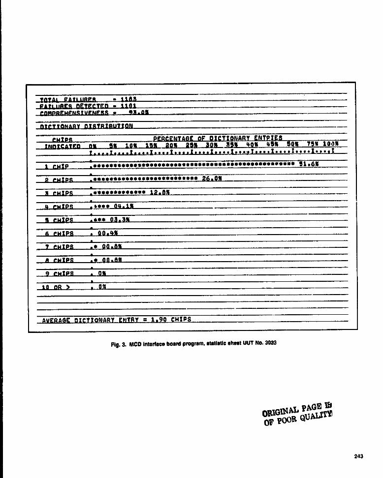
TATM ^A1Ll1R@iR • LiA3
.^1tl.ijrRa fl—TECTIEo .11011
SiCTTOm ARY ntSTRIALITLON -_
i wIP irrwrr^rrrrrrrrrrrrrrrrrrrrrrrrrrrrrrrrrrrrrrrrrrr 01.6!1
wlrm rrrrrrrrsrrrrrrrrrrrrrrerr 26.011
3 rwlpA rrrrrrrrrrr*r 12.A11
4 SHIPS .ersr Oy.ifU
s CHIPS . rrr 03.31E
6 CHIPS 00."
9 CHIPS . r OO.Afi -
® HIPS .• 805S
9 CHIPS 091
----10 C ^ all
AVERAGE DICTIONARY ENTRY a 1.90 CMIPS
Fig. 3. MCD Interface board program, statistic sheet UUT No. 3083
pRIG1N^' PAGElb
OF ?OOR QU ALTM
243

__23 a eCATI Ilar—q nETFGTEn " P %A:2
IST)jrhlrAA - 94_ glob
DICXT3 t ARY pICTRtBl1T ON
CMIAS FERCENTAAE OF DICTIONARY ENTRIES=Atg)=rATFn AA RN to!l Ism 20% as 3 % 35% 404 45% 00% 7398 100%
L- -I- -t- - •L...i....i....I.... ^...I....I....I....i....i
tF1LP r••+ s*+s sssrti^ sss *+rrsss** rs*s*ssse. *+rs.s *rs*oaws^ *s 68.0%
2 rM T RA 17.82
— 3 CMIPC 03.6%
!4 rWPPC .ts ei.44b
b t^IP4 .* ei.2sa
® tF1IP R ne.2^x —
9_CIATIM
Le OR it 00.2%
AvERACE nICTIONARY ENTRY = 1.70 CHIPS
Fig. 4. MCD decoder board program, statistic sheet UUT No. 8803
244

DSN Progrm Rdporl 42-44
January and February 1978
N78-24239
Performance of Solar-Powered Vapor-Jet RefrigerationSystems with Selected working Fluids
V. W. Chai and F. L. LansingDSN Engineering Section
The performance of the solar-powered vapor Jet refrigeration scheme is compared withfire selected working fluids: R-11, R-12, R-113, Butane and Water These fluids wereselected among those able to suit both a power cych! and a refrigeration cycle. The resultsindicated that water has the highest coefficient of performance and differs by a widemargin compared to the other compound organic• fluids at all boiler and evaporatortemperatures considered.
I. IntroductionOne of the objectives of the on-going DSN Energy Con-
servation Project at the Deep Space Communication Complex(GDSCC), Goldstone, California, is to reduce the purchasedenergy by using alternate nondepletable sources such as solarenergy. Heating, v°ntilation, and air-conditioning (HVAC)systems consume about 30 percent of the total energy con-sumption and their coupling with solar energy presents apotential saving. It has been shown earlier (Ref. I) that thesolar-powered vapor-jet refrigeration system (Fig. 1) possessesan overall coefficient of performance comparable with thatobtained from solar-absorption systems or solar-poweredRankine turbo-compressor systems. However, little has beendone in the literature to explore the potential use of solar-jetrefrigeration systems. and it is the intent of this article to helpshed some light on the subject. Conceptually, the solar-jetrefrigeration. scheme as sketched in Fig. 1 is similar to solar-powered Rankine turbo-compressor scheme in which aRankine-power cycle drives a vapor-compression refrigerationcycle. The former scheme uses a nozzle-diffuser ejector for the
expansion-compression processes instead of the combinedturbine compressor unit used in the latter scheme.
Another important difference between the two schemes isthat the ejector scheme can only operate with a single typeFluid while the turbine-compressor scheme can work with dualfluid loops. Consequently, it is very important to carefullyselect the working fluid which best obtains not only a highpower cycle efficiency, but a high coefficient of performance(COP) for the refrigeration cycle also. Other than water as theworking fluid (Ref. 1), Anderson (Ref. 2) used butane gaswhile Kakabaev and Davletov (Ref. 3) used freon refrigerant12 in their jet refrigeration studies. Neither stated the rationalebehind using the chosen chemical as the working fluid.
in the literature, various working fluids for Rankine powercycle alone or refrigeration cycles alone have been studiedextensively (Ref. 4, 5, 7). However, the selection of fluids tosuit both a power cycle and a refrigeration cycle has not beenexplored enough, despite the recent interest in solar Rankineturbo-compressor refrigeration systems.
245

Criteria for Working Fluid SelectionThere are literally hundreds of organic compounds that can
be used as working fluids. Some are only suitable for powercycles which require chemical stability at high boiler tempera-ture while others are only suitable for refrigeration cycles thatoperate at very low temperature ranges without freezing.Before selecting the candidate fluids that have properties suit-able to both a power cycle and a refrigeration cycle to be usedin the solar jet refrigeration system analysis, it is worthwhile toconsider the selection criteria. The fluid thermal behaviorwhich maximizes the system coefficient of performance (COP)an ,l satisfies these criteria will be selected. The selection crite-ria are listed as follows:
First, the availability of' the fluid and the associated cost. Afluid which may result in a very high performance, but haslimited resources or is scarcely found would mean a high costfur the system.
Second, candidate fluids should have a relatively high criti-cal temperature and pressure which raises the high limit for theboiler temperature. A boiler temperature of 93.3°C (200°F)for example, means that many fluids having low criticaltemperatures such as refrigerant-13 (T critical = 29°C) wouldbe operating at supercritical conditions. Supercritical opera-tion requires a careful nozzle/diffuser design. The boiler toevaporator pressure ratio will also affect the nozzle design. Forexample, for superheated steam, if the back pressure is lowerthan 54.6 percent of the boiler stagnation pressure, the nuzzlemust be convergent-divergent with supersonic flow. Without aproper nozzle/diffuser design. under-expansion or over-expansion will occur, which decreases the isentropic effi-ciency.
Third, thermal and chemical stability under cycling be-tween hot and cold regions is an(,ther criterion controlling thehighest bi.;iler temperature fur longer operation.
Fourth, for sate operation candidate fluids should be com-patible with surrounding materials such as copper, iron, rubberseals, etc.
Fifth, fluids should not have excessive boiler pressures ortoo low condensing pressures. F,)r a particular boiler tempera-ture, the saturation pressure should not be too High, to preventleakage problems, and eliminate the need for heavy compo-nents. Also, condenser or evaporator pressures should not betoo low in order to avoid air leakage into the system. Thecondenser to evaporator pressure ratio should be within allow-able limits to assist in an efficient diffuser design.
Sixth, the slope of the vapor saturation curve on thetemperature-entropy diagram should be as steep as possible.
This slope defines the exit conditions of the expansion andcompression processes, and consequently affects the flow ratesof the system. For isentropic expansion or compression, withfluid having a negative slope, exit conditions will be wet vaporat tire end of the expansion process and superheated vapor atthe end of the compression process as shown in Fig. 2a.Conversely, for a positive slope vapor saturation curve asshown in Fig. 2b, the opposite conditions take place. It istherefore preferable to use a fluid having a steep slope for itsvapor saturation curve. The slope should not be greatlydeviated front vertical to avoid extreme conditions.
Seventh, include other operational safety criteria suchtoxicity, flammability, and chemical reactions with air orwater. Finally, the candidate fluid should have high heattransfer coefficient within the temperature range of operation.This property reduces the heat transfer area required for thesolar collector, condenser and evaporator heat exchangers.
III. Selected Working FluidsBased on the above criteria mentioned, five fluids are
chosen for investigation, and their properties are listed inTable I. These selected fluids are known to be suitable inother solar-powered air-conditioning schemes. Stearn refrig-eration is a well known technology and it has been widely usedin industry for some time before the use of mechanically-driven vapor-compression refrigeration. Water has its wellknown advantages. However, it is limited to temperaturesabove its freezing temperature. Also, evaporator operation.with water, at low temperature and pressure has resulted inhigh specific volumes which required bulky equipment. Refrig-erant-12 was used later in the freon ejector solar cooler re-ported by Kakabaev and Davletov (Ref. 3). With a boilertemperature ranging front to 80T. a condenser tempera-ture at 38 00 and an evaporation temperature of 18 0C. the
coefficient of performance (COP) ranged from 0.3 to 0.7depending oil cooling load and the mass flow ratio be-tween the high pressure vapor into the nozzle and the lowpressure vapor from the evaporator. Accordingly. IZ-12 isselected in this work as a prospective candidate to be com-pared with water.
Giancardi, Mender, Blecher and Ilall (Ref. 6) used refrig-erant-1 1 in their turbo-compressor mot. A COP of about 1.0was achieved with turb`.rre inlet temperature of 115.55°C(240 0 F). Refrigerant-1 I resulted in not only a high COP butalso proved itself adequate in both power cycle and ref -rigera-tion cycle combination. Therefore, R-1I is selectee.' in thisstudy as another candidate fluid to be added to the above list.
Barber Wet'. 4) used both refrigerant-1 2 and refrigerant-I 13for the dual fluid solar-powered Rankine turbocompressor
246
cycle. Refrigerant-113 is often considered as a power cyclefluid (Ref. 5) for its high critical temperature. Refrigerant-I 13is then added to the list since it has also a high thermalstability at temperatures up to 500°C.
Finally, after Anderson (Ref. 2), butane is considered acandidate fluid for the study. With butane, the performancewas shown in Reference 2 to be comparable with that of theRankine turbocompressor system and the ejector system canoperate at lower supply temperatures than that for solarabsorption system.
IV. Performance Comparison With theSelected Working Fluids
The five working fluid candidates namely; water, R- 11,R-12, R-113 and Butane are tried each in a jet refrigerationcycle under identical evaporator, condenser and boilertemperatures. The objectives were set to determine the trendof the cycle coefficient of verformance with (I) various boilertemperatures keeping all other parameters the same and(2) various evaporator temperatures keeping all other param-eters the same.
The isentropic efficiency for each of the nozzle and thediffuser is kept unchanged in the study. Since the condensertemperature can vary only with the type of cooling nediurnwhether it is air or water, and ambient conditions, the con-denser temperature was considered a fixed parameter notaffecting the final fluid choice. Oil other hand, the boilertemperature is considered an important parameter since it iscontrolled by the maximum stable temperature the fluid canhandle. The evaporator temperature is also important since itis controlled by the fluid freezing temperature.
The results of the parametrization study are plotted inFigures 3 and 4 using the fluid thermodynamic properties inReference 8 and the nomogram methodology previously re-ported ip Reference 1. Figure 3 shows the coefficient of per-formance (COP) versus the evaporator temperature for the fiveworking fluids with all other parameters fixed. Since watercannot operate below 0°C, the evaporator temperature rangewas taken between 4.44°C (40°F) and 15.56°C (60 0 F). FromFig. 3, the higher the evaporator temperature, the higher theCOP which is ail result derived from the idealCarnot's performance.
It is also evident from Fig. 3 that the COP for fluids R-I I,R-12, R-I 13 and Butane lie within a narrow band much lowerthan that for water. For example, at 10°C (50°F) evaporatortemperature. the COP for the organic fluids tested varied front0.4 to R-i 1 to 0.47 for R-113 compared to 0.85 for water at
the same conditions: a result which makes water a fluid withexcellent performance,
In Fig. 4, the COP results were plotted with fixed evapora-tor temperature versus the boiler temperature. Boiler tempera-tures were ch... .en between 80°C (176'F) and 1 10°C (2300F)to suit most low cost flat-plate collectors. Theoretically for theCarnot refrigeration cycle, the COP increases with increasingthe high source temperature (boiling temperature) and thetrends in Fig.4 for water follow the theoretical trend. How-ever, for refrigerant-I I and refrigerant-I 13, the COP reaches amaximum at about 95°C with COP at about 0.35 for R-I 13and 0.32 for R-12. For refrigerant-12 the COP increases withincreasing boiler temperature, but its relatively low criticaltemperature ( — I 100 C) prevents it from operating at highertemperature values.
Also from Fig. 4, steam has the highest COP among thefluids selected, which is contributed mainly by its large latentheat of vaporization. On the other hand, steam required bulkycomponents to handle the large volumes of flow since it has avery large specific volume compared to organic compounds atthe same temperature.
V. Summary and FindingsFrom this study, the following findings can be drawn:
The performance of the solar-powered vapor-jet refrigera-tior,. sL;henie was tested with five selected working fluids:.R-i I, R-12, R-i 13, Butane and water, using the nomogrammethodology constructed earlier in Reference I.
The proper selection of the working fluid is subject tomany selection criteria such as ( I ) fluid availability and lowcost, (2) high critical temperature (3) thermal and chemicalstability under hot/cold cycling (4) compatibility withother surrounding materials (5) low saturation pressures,(6) steep slope of vapor-saturation curve oil
diagram (7) nonflanmaability, toxicity properties,and (8) high heat transfer coefficient.
3. All five working fluids selected have an increasing trend ofCOP with the evaporator temperature. The increasing trendcould be reasoned by the similar Carnot's behavior. How-ever, the resulting COP had two distinct bands separated bya large margin: water performance in one side and all theother organic compounds in a narrow band. Water wasshown superior than the other organic fluids with a (COP)almost double the value obtained from the other fluids.
4. With the boiler temperature as a parameter, refrigerantsR-1 i and R 13 reached a maximum (COP) value at about95°C but water and R-12 had a monotonic trend. Again.
247
the water (COP) was superior compared to other organiccompounds. The large latent heat of vaporization that thewater possesses in addition to the odd-shaped and smallvapor curve slopes that the organic compounds have on thetemperature-entropy diagram contributed to the water per-formance superiority.
Although water, as a fluid, has the disadvantage of largespecific volume at low temperatures which tend to increasethe component size, besides its low freezing temperaturewhich requires careful handling and design, it is foreseenthat water will be selected as the only candidate in futurestudies of solar-powered vapor-jet refrigeration schemes.
References
I. Lansing, F. L., Chai, V. W., "A Thermodynamic Analysis of a Solar-powered JetRefrigeration System". DSN Progress Report 42-41, Jet Propulsion Laboratory,Oct. 15, 1977, pp. 209.217.
2. Anderson, H., "Assessment of Solar Powered Vapor Jet Air-conditioning System".Presented at 1975 International Solar Energy Congress and Exposition (ISES) held atUCLA, Los Angeles, California, p 408.
3. Kakabaev, A., Davletov, A., "A Freon Ejector Solar Cooler". Geliotekhn:ka, vol. 2,No. 5, pp. 42 .48, 1966.
4. Barber, R. E., "Solar Air Conditioning System Using Rankine Power Cycles — Designand Test Results of Prototype Three Ton Unit". Institute of Environmental Science,1975, pp. 170.179.
5. Miller, D. R., "Rankine Cycle Working Fluids for Solar-to-electrical Energy Conver-sion". Final report for Sandia Laboratory, Albuquerque, New Mexico, January, 1974.
6. Biancardi, F. R., Meader, M. D., Blecher, W. A., and Hall, J. B., "Design and Operationof Solar-powered Turbocom pressor Air-conditioning and Heating System" IECEC '75Record, pp. 186.194.
7. Allen, R. A., Stiel, L. I., "Working Fluids for Solar Rankine Heat Pumps". SolarEnergy Heat Pump Systems for Heating and Cooling Buildings. ERDA Doc. coo-2560-1, 1975, pp. 98-105.
8. ASHRAE Handbook of Fundamentals, American Society of Heating, Refrigeratingand Air Conditioning Engineers, Inc., New York, New York 1972.
ORIGINAL PAGE IS
OF POOR, QUALM248

Table I. Sonve properties of the selected fl%:lds
I 2 1 Specific Flauuuablc urSelected Critical Critical Molecular Boiler CUI1dOnxef I'.V:IIh)i:11OI' Volume a! l`\pIUxIVCWorking Temperature Pressure Weight Pressure Pressure ,Pressure
Condenser units in airFluids Cc) (atm) (gill /gill-n ► Ole) tn
(ahn) loon) (atm)'Tem perature
(Ill'/kg)l" by volume)
Sleanl 374 218 18.02 .78 .034 .0008 12.80 non Ilannnabie
Refrigerant-11 198 43.2 137.38 6.97 1.10 .48 .098 non•Ilanunable
Refrigerant- 12 112 40.6 120.93 29.26 6.73 3.51 .014 noll-fl:un Ina tile
Refrigerant-113 214 33.7 187.39 3.72 .47 .18 .208 non-flammable
Butane 152 37.46 58.13 13.25 2.53 1.20 .085 1.6 to 6.5
I Boiler Temperature 93.3°('(2(10"1)2 Condenser Temperature 26.67°('(811°1:)3 Fvaporalor Temperature 4.44'('(40" F)
249
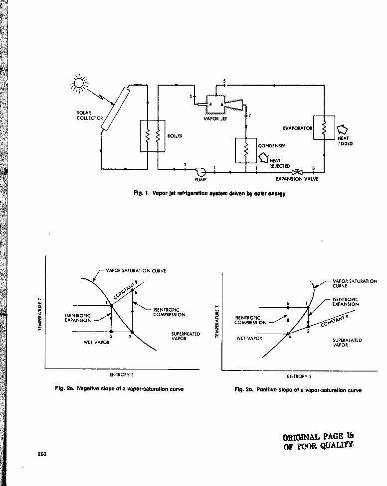
s
SaeCOLI
HEAT'DDED
W
PUMP EXPANSION VALVE
Fig. 1. Vapor het refrigeration system driven by solar energy
VAPOR SATURATION CURVE
VAPOR SATURATIONCURVE
bCO ISENTROPIC
_ I b I EXPANSIONISENTROPIC W
ISENTROPIC COMPRESSION ISENTROPIC r1t?EXPANSION ° COMPRESSION CONStP
SUPERHEATED 2
WET VAPOR 1 ° VAPOR '' WET VAPOR ° SUPERHEATEDVAPOR
ENTROPY S ENTROPY S
Fig. 2a. Negative slope of a vapor -saturation curve Fig. 2b. Positive slope of a vapor -saturation curve
ORIGINAL PAGE lbOF PrV)R QUALM
250
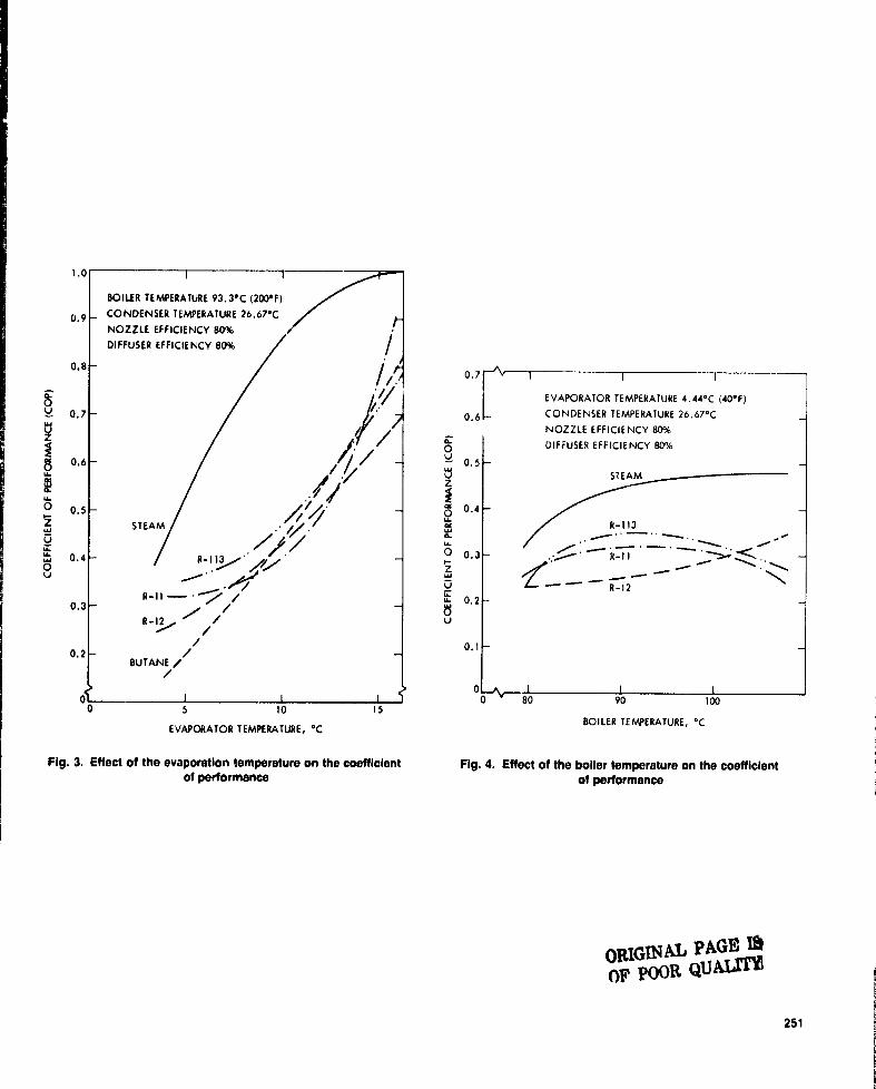
OVW
ffi
O
LL
0
I,0 I-I
BOILER TEMPERATURE 93.3-C (200-F)0 . 9 CONDENSER TEMPERATURE 26.67-C
NOZZLE EFFICIENCY 80%DIFFUSER EFFICIENCY 80%
0.8
0.7
l0.6
0.5 STEAM
0.4 R-113
R-11 — • ^ /0.3-/
0.2 /BUTANE
5 10 15
EVAPORATOR TEMPERATURE, -C
Fig. 3. Effect of the evaporation temperature on the coefficientof performance
0.7 "—j— —
EVAPORATOR TEMPERATURE 4.44-C (40-F)
0.6 CONDENSER TEMPERATURE 26.67-CNOZZLE EFFICIENCY 80%
00 DIFFUSER EFFICIENCY 80%v 0.5
ZSTEAM
I0
0,4
R-113
O 0.3
Zu L — -- — R-12
0.2
U
0.1
0 ' 80 90 100
BOILER TEMPERATURE, -C
Fig. 4. Effect of the boiler temperature on the coefficientof performance
ORIGINAL PAGE^OF POOR
251

DSN Progress Report 42.44
January and February 1978
N78_24240
Voyager Neer Simultaneous Ranging 'TransfersG. L. Spradlin
Deep Space Network Operations Section
During testing of near simultaneous ranging technique~, a major shortcoming of thestandard USN uplink transfer procedure was uncovered. Use of the standard procedureresulted in loss of phase coherence between received and reference range codes for theround trip light time fbIlowing a transfer. It is the intent of this article to report on thephilosoph ►v behind, and the operational procedure developed for ►tear simultaneous rangetransfers, a new uplink transfer procedure that will enable the DSN to generate goodrange data during the interval fro ►n transmitter off to loss of the coherent downlink.
I. IntroductionA unfortunate geometry, zero declination, will exist at
Saturn encounter for both Voyagers. This geometry will make
it impossible to solve for the spacecraft's declination by fitting
doppler data as is normally done in the orbit determination
process. An alternative technique for deriving the spacecraft's
declination is by use of range data taken near simultaneously
from stations at widely separated latitudes, and triangulating
to solve for the needed declination angle. This dependence
upon range data will require that highly accurate range mea-
surements and range delay calibration information be available
to the navigators and radio scientists. It has been towards this
end that countless hours have been (and continue to be) spent
proving and refining network ranging procedures and analyti-
cal techniques for data quality verification.
Periodic tests of the near simultaneous ranging (NSR) tech-
nique were conducted during late 1976 and early 1977. The
purpose of these tests was to verify that the range accuracy
requirements for Voyager navigation could be met, and also to
develop the operational procedures that would be imposed on
the DSN by this new data collection scheme. The results of
these tests are the subject of Reference I .
As a result of analysis of the data collected during the near
simultaneous ranging tests (and noted in Ref. 1), it was dis-
covered that standard USN procedures for station-to-station
uplink handovers had resulted in loss of range code phase
coherence, and hence !oss of range data during the round trip
light time following a handover. It was suggested that phase
compensatory tuning might be utilized by the network to
solve this problem, and prevent the loss of range data after
uplink handovers,
in support of the ne. r simultaneous range data collection
effort, the DSN has accepted the phase compensatory tuning
recommerdatimi, and developed operational procedures for
carrying it out. The remainder of this article describes this
plan, and l:iesents the operational procedure that the network
will be utilizing in support of the near simultaneous ranging
effort.
II. NSR Transfer PhilosophyEvery two weeks, once a month per spacecraft, the Voyager
Project is planning to gather navigation and radio science data
(S-band doppler and range data, and X-band doppler and range
252

when available) by means of a "tracking cycle". The trackingcycle consists of four consecutive 64•n ►eter antenna tracksbeginning with DSS 43 and ending with DSS 43. It should benoted, however, that an attempt to collect NSR data may bemade whenever two DSS% are scheduled simultaneously totrack a single Voyager spacecraft; this includes colocated sta-tions, and stations of the same general view period (64-meterand/or 26-meter antennas).
The data of prime importance during the tracking cycles (orother simultaneous tracking periods) are the NSR data. Duringthese overlaps, attempts will be made to maximize the returnof high quality two- and three-way doppler and NSR measure-ments. Since two stations cannot concurrently have sustaineduplinks with a single spacecraft, collection of the NSR datawill require that numerous uplink transfers be made during theoverlaps to provide data redundancy and hence daiaconfidence.
These numerous transfers present more of a problem forthe network than a cursory glance might reveal. The "stan-dard" DSN transfer, where: (I ) the incoming DSS and theoutgoing DSS both tune to the spacecraft's receiver VCOcenter frequency, XA, (adjusted for one-way doppler and lighttime); (2) the incoming DSS turns on its transmitter and theoutgoing DSS turns its off two seconds later, and (3) the DSSsboth tune to their respective Track Synthesizer Frequencies(TSFS) and remain there until the end of the track or the nexttransfer, cannot generally be used for uplink transfers whileNSR data are being generated. This tuning pattern, whileadequate to transfer the uplink, will change the phase relation-ship of the ground reference and received range codes, and willthus result in the loss of' range data from the outgoing DSS forthe round trip light time. To avoid this loss of NSR data, analternate tuning procedure has been developed.
The new transfer procedure that has resulted from analysisof the problem will, upon completion of all required tuning,restore both the frequency and code phase relationshipsrequired for good ranging throughout the round trip light timefollowing an uplink transfer. The only data loss is that duringthe period of the tuning. This transfer procedure, dubbed theNSR transfer, takes advantage of the programming and preci-sion tuning capabilities of the Programmed Oscillator ControlAssembly (POCA) available at the 64-meter DSSs. The proce-dure calls for both incoming and outgoing DSSs tc executeprecision symmetrical tuning patterns between specified limits,at fixed rates, and at specific times. Figure I graphicallydepicts a NSR transfer and its related events.
In Fig. I, it can be seen that the transfer procedure requiresutilization of four ramps to achieve the desired symmetricaltuning pattern. All ramps are dime at the same rate, 5 IIz/sec
(POCA); the initial direction of the first ramp is dependentupon whether XA is above or below TSF. The distance tuned,OHZ, is simply
AHZ = XA - TSF
Since the XA is a doppler dependent frequency, it con•stantly changes. Therefore the AHZ for any given transfer timewill be different. That is, sometimes a sweep of +30 HZ will berequired, or +2.1 HZ or -12.4 FIZ, etc, It is for this reason thatthe upper and lower limit registers of the POCA are used;otherwise, new rates and ramp start (lines would have to bedetermined for each transfer to account for the differentdistances to be tuned, and to retain the desired symmetry. Asfour frequencies are needed for POCA limits: TSF + DMZ,TSF, TSF - AHZ. TSF, and they must be encountered in thissequence, it will be necessary to reload each POCA limit onceduring the transfer sequence, Nominal times for these updateshave been indicated at transfer + 1 min. 20 sec., and at transfer+ 2 min. 40 sec.
In Fig. I, ULI and LLI represent the initial upper andlower limits respectively. (Note: if AHZ is a negative numberthe first sweep will be in the direction of a lower frequencyand U.l.) UL2 and LL2 represent the updated POCA limits.The Ts and Rs represent the contents of the four POCArate/time registers with all rates at either plus or minus5 I-lz/sec. (POCA) (as appropriate) and times as follows:
TO = Time of transfer minus I minuteTI = Time of transfer plus I minuteT2 = Timc of transfer plus 2 minutesT3 = Time of transfer plus 4 minutes
T'he total time to execute the entire transfer and tuningpattern is approximately 5 minutes with the time changing bya few seconds depending upon the magnitude of O1IZ.
Other events indicated are the actual transfer tittle, it d theincoming and outgoing range modulation on/off times. Trans-nutter oil the incoming DSS is at the even minute followedby transmitter off two seconds later at the outgoing DSS.Transfer time is defined as the time of transmitter on at theincoming station. Range data prior to the first ramp start timemay be of value; therefore, range modulation at the outgoingstation will not be turned off until a convenient time after thestart of tuning (range modulation off at transfer -20 sec, nom•inally ). Similarly, range modulation at the incoming DSS is notapplied until tutting is complete (nominally, range modulationon :.t transfer + 4 min. 10 sec.).
253

Clearly, the NSR transfer requires the use of a POCA. Wheutransfers are required for the collection of NSR data where aPOCA is not available a "standard" transfer is to be executed.Or, in the unique case of DSS 12 and DSS 14, a TSF transfer isto be used. (DSS 12 and DSS 14 are unique in that they areeach equipped with a ranging subsystem unlike USSs 42/43and 61/63 where ranging systems are shared, also USSs 12 and14 are close enough that tuning for transfer is unnecessary,i.e., almost identical doppler shifts.)
While it is unfortunate that the network must adapt to anew transfer procedure in support of NSR data collection, itshould be noted that development of a fixed procedure hasbeen one of the design goals in an effort to make the requiredadaptation as painless as possible.
The uplink tuning rate selected, 240liz/sev (S-hand), iscompatible with Voyager Telecommunications provided signallevel estimates for Jupiter Encounter (and beyond), Groundreceiver tuning will be avoided by:
(I ) Selection of the 30 . 1Iz-wide bandwidth at the Block IVReceive r• Exciter Subsystem, and,
(2) 'Zeroing the Static Phase Error (SPE) of tine teceiversprior to beginning the NSR transfer sequence.
111. (ASR Transfer Procedure
To aid in the transfer of information, a new transfer mes-sage, the NSR TRANSFER MESSAGE (Fig. 2) has been de-signed. This form provides all needed information (frequenciesand event times) for buff ► in.on ► ing and outgoing stations. Theblanks on the NSR TRANSFER MESSAGE are to be filled inby the Network Operations Control Team (NOCT), To assistin completing the form, all calculator program hasbeen written that, given the inputs necessary for a "standard"transfer, will convert thew to (also, output) NSR transferinformation required to complete the form. Section IV pro-vides an example of how tl ► e prograrn and transfer message areto be utilized.
The same considerations utilized for deternnii,mr, moptimal tuning strategy were also used in determining it
strategy. It is not anticipated that ranging parameters willbe altered prior to encounter. Arrangements have been madeto provide these inputs through the Sequence of Events (SOL).A line item will be provided that will warn of an approachingoverlap period, and provide some general reminders includingthe necessary range parameters. It is of paramount importancethat the Planetary Ranging Assembly (PRA) not be inter-rupted during the overlap period; this is regardless of thetransmitter or range modulation status. Any and all inputs.
such as a round-trip light time (RTLT) update, must be madeprior to the critical data collection period.
The SOL items will include, in addition to the abovementioned ranging parameters:
( I ) A statement that announces the beginning of the NSRdata collection period, and provides initial conditions.
(2) A wanting of an approaching period of NSR transfersthat should be a trigger to the NOCI oil thenecessary NSR TRANSFER MESSAGE(:.).
13) A statement to commence multiple NSR transfers, theGMT of this statement should coincide with the firsttransfer.
(4) A statement that announces the end of a NSR transferperiod.
The following items should be remembered as they .'rectlyimpact the NSR data:
( I ) Frequent uplink transfers will result in frequent dop•pler mode (two-way vs, three-way) changes; the NOCTroust be careful that the correct node is indicated toavoid extensive data editing.
(2) The good/bad doppler switch (manual) should be set toIndicate had doppler data during uplink tuning, andone RTLT later when the tuning is received in thedownlink. This will again eliminate the need for dataediting.
(3) The dop pler sample rate should be set to one sampleper ten seconds during all trans fer periods, It should beleft at one sample per tell continuously at64-niter DSSs throughout the tracking cycle.
(4) NSR transfers should be performed oil min-ute centers:
(a) Beginning at tell elevation (64-nnetet antes•nas) or at the indicated SOL start time whichever islater,
(b) At the midpoint of the DSS 43163 overlap •mtilthe overlap exceeds approximately two hours(three NSR transfers).
(c) And an odd number of NSR transfersalwaYs mustIle completer) (3, 5 etc.),
(d ) And no more than five transfers are to be at-tempted during 64-meter overlaps. More transfersmay be requested during DSS 12/14 NSR datacollection periods. The maximum number maylater be reduced t o three transfers during 64-meteroverlaps.
254

In addition to providing the NOCT with the aforenten-tioned IIN 0810 program, a program copy will be provided toeach 64•nitter DSS, This should help expedite the transfer ofNSR transfer information. It is not necessary for tacit DSS tohave the XA and TSF of the other involved DSS, Zeros may beentered in the program for inputs relative to the other station;this will not affect the NSR transfer information output forthe station utilizing the program. It is further suggested thatthe DSSs adopt the NSR TRANSFER MESSAGE form as arecording medii-11
IV. Example
A SOE item that indicates the beginning of a NSR multipletransfer period has been noted. At a convenient time, about anhour prior to the noted SOE item the NSR TRANSFERMESSAGE for the first transfer is prepared. This first transfertime is to be 235000; this is somewhat later than the eventtime of the SOF, but is the first predicts data point availableafter ten degrees (10°) of elevation angle has been reached.DSS 14 is outgoing and is currently at a TSF of 44028500 Hz.Thr transfer will be to DSS 43 whose TSF will also be44028500 Hz. From the tracking predicts the respective trans-fer time (23:50:00) XAs are found to be:
XA (14) = 44028546.1 FIz
XA (43) = 44028490.9 fiz
Now load the NSR TRANSFER .'ROGRAM into the III'9810 calculator, and simply enter the data r.quested by theprogram (Fig, 3) as lollows:
(I ) "XFER GMT -" enter the transfer time, 23:50:00
(2) "OUTGOING TSF =" enter DSS 14's TSF, 44028500
(3) "OUTGOING XA enter DSS 14's XA, 44028546.7
(4) "INCOMING 1 SF enter DSS 43's TSF, 44028500
(5) "INCOMING XA enter DSS 43's XA, 44028490.9
(6) The NSR TRANSFER MESSAGE is now filled outfrom the program output, ,ind then either read or faxedor both to the involved DSSs. The DSSs should bereminded of the notes at the bottom of the fonts (Fig.4) as they are important to the successful completionof the NSR transfer.
Once the program card becomes available at the 64-meterDSSs, it may prove most expeditious to simply verify that theOSSs have arrived at the same frequencies as those computedby the NOCT. Each DSS will have available its own TSF andXA, but not those of the ether involved DSS; therefore,comparison of results will be limited to only those items thatdirectly apply to that DSS.
Reference
I. It L. Siegel, C. S. Christensen, D. W. Green, F. R. Winn, "On Achieving SufficientDual Station Range Axuracy for Deep Space Navigation at Zero Declination,"AIAA/AAS Astrodynamic Specialists Conference, Jackson Hole, Wyoming, September7.9, 1977.
255

R3
TIME (MIN) — 1 1 2 3
Z—^—T—
TRANSFER --41^ UPDATE POCA
RANGE MOD OFF LIMIT(OUTGOING) "'iUPDATE POCA RANGE MOD ONLIMIT (INCOMING)
ULI TIRo 2 1
AHZ T2 UL2 —^
TSF i
TO LL IAHZ
R2r- LL2
NOTES: ^— T3I . pHs = XA (OF TRANSFER) - TSF, COMPUTED TO ONE TENTH H:2. ALL TUNING RATES ARE 5 Ha/sec, THE SIGN ON RO 6 R3 IS THE
SAME AS THAT OF AHaTHE SIGN ON RI 6 R2 IS OPPOSITE
THAT OF AH:3. ULI = POCA INITIAL UPPER LIMIT FREQUENCY = TSF +(AHa)4. LLI = POCA INITIAL LOWER LIMIT FREQUENCY = TSF = UL25. LL2 = TSF - (AH:)6. TO = TIME OF TRANSFER - 1 min7. TI = TIME OF TRANSFER + 1 minB. T2 = TIME OF TRANSFER + 2 min9. T3 = TIME OF TRANSFER + 4 min
10. PRA MUST NOT BE INTERRUPTED REGARDLESS TRANSMITTER OR RANGE MOD STATUS11. DOPPLER SAMPLE INTERVAL - 10 sac12. RECEIVER BANDWIDTHS SET 30 H:-WIDE, NO TUNING AT TRANSFER REQUIRED13. TRANSFERS TO OCCUR ON 35 min CENTERS
Fig. 1. NSR transfer and related events
TSF
258
r
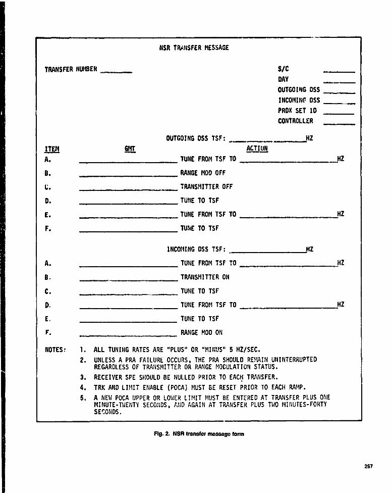
NSR TRANSFER MESSAGE
TRANSFER NUMBER
S/C
DAY
OUTGOING DSS
INCOMING DSS
PRDX SET 1D
CONTROLLER
OUTGOING DSS TSF: HZ
ITE14 GMT ACTION
A. TUNE FROM TSF TO ^HZ
B. RANGE MOD OFF
G. TRANSMITTER OFF
D. TUNE TO TSF
E. TUNE FROM TSF TO HZ
F. TUBE TO TSF
INCO14ING DSS TSF: HZ
A. TUNE FROM TSF TO HZ
B. TRANSMITTER ON
C. TUNE TO TSF
D. TUNE FROM TSF TO HZ
E. TUNE TO TSF
F. RANGE MOD ON
NOTES: 1. ALL TUNING RATES ARE "PLUS" OR "MINUS" 5 HZ/SEC.
2. UNLESS A PRA FAILURE OCCURS, THE PRA SHOULD REMAIN UNINTERRUPTEDREGARDLESS OF TRANSMITTER OR RANGE MODULATION STATUS.
3. RECEIVER SPE SHOULD BE NULLED PRIOR TO EACH TRANSFER.
4. TRK AND LIMIT ENABLE (POCA) MUST BE RESET PRIOR TO EACH RAMP.
5. A NEW POCA UPPER OR LOWER LIMIT MUST BE ENTERED AT TRANSFER PLUS ONEMINUTE-TWENTY SECONDS, AIiD AGAIN AT TRANSFER PLUS TWO MINUTES-FORTYSECONDS.
Fig. 2. NSR transfer message form
257

TPANSF E - PPOGF'RI-I
XFER GMT=235000.0
OUTGOINi: T,.--.F=
44028500.0*OUTGOING
44028541.7*INCOMINC TSF=
44020500,0*INCOMING -'.'Fi=
44028490.9*
OUTGOING DSSITEMS 1`4 THF'U F
234900.044028546.7
234940.0
235002.0
235100. 0
2-13, 5200. 04406:,4 5'3• 3
I N 01 l- 1 11 11: TiITEMS A THRI-1 F
2'^.: 4 9 C-1 0 . 04 4 9 0 • 9
2..'5 C, 0 0 . C,
351 C1 11. Cl
04 . C, C., 5 0 9 . 1
2 "*0 .1 A cl . 0
2 51 .1 1 0 . C1
Fig. 3. Example of program output ORIGINAL PAGE LbOF POOR QUALI=
258
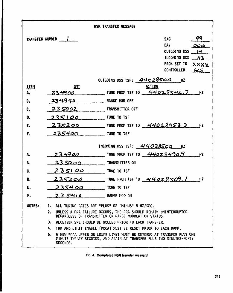
NSR TRANSFER MESSAGE
TRANSFER NUMBER I_ S/C 99DAY O o p
OUTGOING DSS .__c,-4INCOMING DSS 1
PRDX SET ID -Y-AxyCONTROLLER &S
OUTGOING DSS TSF: 1q4g021?5'00 HZ
ITE14 GMT ACTION
A. Z3 6J9 Q0 TUNE FROM TSF TO ±f Al 0 Z $ -45ti (a . 7 HZ
B. 23 -49 4 0 RANGE MOD OFF
C. 2 3 Sly dL TRANSMITTER OFF
0. 2 3 S' / O Q _ TUNE TO TSF
E. 7. .352 O0 TUNE FROM TSF TO A1 .400 AI S3.3 HZ
F. a3 S"'E Oti TUNE TO TSF
INCOMING DSS TSF: -'102-80CZ HZ
A. y9 00 TUNE FROM TSF TO "O2 9±j'jQ.9_ HZ
B. 2-3 50 O 0 TRANSMITTER ON
C. 2- 3 $'1 O G) TUNE TO TSF
D. Z .52 0 TUNE FROM TSF TO e4 DZ- 9,TQ!j. / HZ
E. 2,35'SI 00 TUNE TO TSF
F. ,. 3 Ste! I a RANGE MOD ON
NOTES: 1. ALL TUNING RATES ARE "PLUS" OR "MINUS" 5 HZ/SEC.
2. UNLESS A PRA FAILURE OCCURS, THE PRA SHOULD REMAIN UNINTERRUPTEDREGARDLESS OF TRANSMITTER OR RANGE MODULATION STATUS.
3. RECEIVER SPE SHOULD BE NULLED PRIOR TO EACH TRANSFER.
4. TRK AND LI11IT ENABLE (POCA) MUST BE RESET PRIOR TO EACH RAMP.
5. A NEW POCA UPPER OR LO.-IER LIMIT BUST BE ENTERED AT TRANSFER PLUS ONEMINUTE-TWENTY SECONDS, AND AGAIN AT TRANSFER PLUS TWO MINUTES-FORTYSECONDS.
Fig. 4. Completed NSR transfer message
259

DSN Progreuy ROW 42-44
January and February 1978
S78-24241
Some Data Relationships Among Diverse Areasof the DSN and JPL
R. M. SmithDSN Support Section
A logical-level data model is used to represent real-world relationships among diverseareas of the Deep Space Network (DSN) and mm-DSN areas. The possibility for reductionofdata redundancy is addressed.
I. Introduction
Section 377 (Deep Space Network Support) maintains anoperational database containing data for managing equipmentused H, Deep Space Network operations. The types of datamaintained are: description, identification, location and sev-eral kinds of status including data on failures, modificationsand shipments. During the past few years, work conducted onthe database has revealed and emphasized the existence ofrelationships in the data domain among diverse elements of theDSN and JPL.
II.Data Relationships
This article presents a cursory analysis of sonic of the datarelationships that exist among various DSN (and JPL, non-DSN) activities. The data elements used in this article arerepresentative of existing real-world attributes. Data elementsets, representing existing real-world entities, are presented inthis article in the form of third-normal-form relations (definedin Ref. I ). The relations and data elements are not necessarilyused as-is in existing databases, rather the intent of theserepreseniaiions is to show the existence of real relationships inthe data domain; hence the possibility for communication and
coordination among the databases of apparently diverseorganizations. The lists of data elements and relations are notexhaustive.
Seven separate functions in the DSN and two non-DSNfunctions are represented by collections of relations toillustrate interrelationships within and beyond the bounds ofthe DSN.
Table I lists all the data elements used in this article anddefines each, as used in the article. Tables 2 through 10 depictrelations applicable to the functions indicated by the tabletitles. Each table may be viewed as a separate, limited logicaldatabase or the entire collection may be viewed as representa-tive of a larger, global logical database.
Within each table call seen one or more data elementsused repeatedly, as common keys, among the relations. Thesecommon keys provide logical links among relations. Were theserelations properly established in a database, a user could makeuse of the existence of the common keys to produce usefulinformation. For instance, using relations 3 and 27 with CONNUMBER as a common key a user could determine thelocation of an item of equipment with a specific JPL Property
260

Number or he could obtain a listing of all property-controlled from LOCATION in relation 3. Casual inspection will revealequipment at a given location. other, similar relationships.
Similar logical links exist among tables (therefore, betweenJPL activities). For instance, CON NUMBER is common toTables 2, 6 and 7; JPL DWG is common to Tables 2, 3, 7 and 4(where DOCUMENT is equivalent to JPL DWG). As a finalexample of the existence of logical links: If the relations wereintegrated in a database, the location of all equipmentauthorized under a given ADP (Automatic Data Processing)Plan could be determined; using ADP ID as an access key inrelation 98; using PO NUMBER as a common key betweenrelations 98 and 1; using CON NUMBER as a common keybetween relations I and 3; deriving resultant location data
III. Redundancies
It is interesting to note the amount of redundancy thatexists throughout Tables 2 through 10. By integrating a,* 99 ofthe relations in Tables 2 through 10, 26 duplicate relationsmay be deleted. An additional 7 relations may be removedbecause of the existence of multiple inferred relationships.This amounts to approximately 33 percent reduction inredundancy as a result of integrating the diverse data sets. Thisis probably typical of the degree of reduction that could beachieved in an actual integration.
Reference
1. Date, C. J., An Introduction to Database Systems, Addison-Wesley PublishingCompany, Inc., Reading, Mass., 1975.
261

Tabu 1. OWlnfttons of data stsmsnta uasd to tables 2 Utrftgh 10
DATA ELEMENT NAME DATA ELEMENT DEFINITION
1—ACCEPTANCE2—AC,ro DATE.3—ADDRESS4—ALP ID
—APPLIC FAC@,—CATEGORY
7—C-DE
:3 — CERT S TATUS9—C ER T _ 1_ E JEC T
1 0—COE REC DATE11 — COE ': HIP DATE12—CUE1'3 — CON NUMBER14 — CW' T15 — E16 — DATE FUNCTIONAL17°DATE18—DELEGATION19—DESCRIPTION20—DESIGN FINISH21 — DE:: ' T FAC22- DI:SCPEPAP4CY2:3—DIZPO`_ITION24—DOCUMENT25. — P! IE DATE26 —EC COST27 —EC EXCEPTION28 — EC TATU':2'3 — EC I:u—ECO1—ECP
'32 —EMP NUMBER—Eh1F ORGRN I ZRT I ON
:34 -'ES:T DES. FINISH—EST FAB FINISH
PEE. — FAB F I N I SH{' — PAC' COMP DATE
— FAC EST COMP39 — FAC PEC DATE4 u — FAC I L I T'('41 —FRIL DATE42 —FRIL TIME43—ICE44— I N Z.P DATE45— INSP NUMBER46 — IN:_P =TAT1,15
ACCEPTANCE STATUS OF EGO FIRST INSTALLATIONDATE ON WHICH PROPERTY WAS ACQUIRED BY •JPLADDRE"S OF P MANUFACTURERADP FLAN IDENTIFICATIONFACILITY TO WHICH AN ENGINEERING CHANGE I, APPLICABLEUSAGE CATEGORY OF EQUIPMENTCOGNI^ANr DEVELOPMENT ENGINEEREMPLOYEE PA TRAINING ' JRTUSSUBJECT IN WHICH AN EMPLOYEE IS CERTIFIEDDATE OFI WHICH A COE RECEIVED AN ECO KITDRTE ON WHICH A COE HIPPED AN ECO KITCOGNI ZANT OPERATION': ENGINEERD:=N EQUIPMENT CONTROL NUMBERC O: T OF AN ITEMCOGNItANT :_USTAINING ENGINEERDATE ON WHICH MODIFIED EQUIPMENT I`_ FUNCTIONALDATE OF AN EVENT OF' CONDITIONFACILITY TO WHICH E! )! i I PMENT MR I NTENRNCE I DELEGATEDDESCRIPTION OF AN ITEMDATE THAT ECO DESIGN 1`-7,FACILITY TO WHICH AN ITEM I:_: BEING SHIPPEDDISC.REPRNC 'r' DIS'CO'-.-ERED DURING INSPECTIONFINAL D I _ F'O : I T I ON OF MATERIAL AFTER INSPECTIONCONTPOLLING IDENTIFICATION OF R DOCUMENTDATE ON WHICH AN EVENT OR CONDITION IS: DUEE:TIMATED TOTAL COST TO IMPLEMENT AN ECOE'CEPTION TO AN ECq FIRST IN:-TALLRTIONEC. T8T1_1^; OF AN ITEM OF EPI J I PMENTENGINEERING CHANGE III=TFSUCTIONENG I PEERING, CHANGE ORDERENGINEERING CHANGE REQUESTJPL EMPLOYEE NUMBERNUMERIC DIVI_^ION—SECTION IDENTIFIERESTIMATED ECO DESIGN F I tI I .=• H DATEE'_TIMATED ECO FABRICATION FINISH DATEDATE THAT ECO FABRICATION IS FINISHEDDATE OF ECO COMPLETION AT A FACILITY
DATE OF ECO COMPLETION T A FACILITYDATE OF ECO k' I T RECEIPT AT R FACILITY D:: PI q PEPRT I ONAL OR :_!IPPORT FACILITYDATE OF E01JIPMENT FAILURETIME OF EQUIPMENT FAILUREIMPLEMENTATION COORDINATION ENGINEERDATE ON WHICH AN INS=PECTION WAS COMPLETEDUN i QUE NUMBER AS :S I GNED TO FIN I N .PECT I ON ACTIVITY: TATU'S. OF AN INSPECTION
262
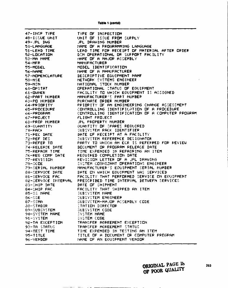
Table 1 (eontd)
47— INSF TYPE TYPE OF IN:sPECTION48-1 UE UNIT UNIT OF IS`UE FROM SUPPLY49—JPL DIAG JPL DRAWING NUMBER50—LANGUAGE (NAME OF A PROGRAMMII •NG LANGUAGE51 —LEAD TIME LEAD TIME FOR RECEIPT OF MATERIAL AFTER ORDER52—LOCATION D'''N OPERATIONAL OR '^IJF PORT FACILITY53 — MA NAME HRME OF A MAJOR A SEMBLY54—MFR MANUFACTURER55—MODEL MODEL IDENTIFICATION56—NAME NHME OF A MANUFACTURER57 —NOMENCLATURE DESC•RIPTIVE EQUIPMENT NAME58—MSE NETWORK `'Y`'TEMS ENGINEEF59-14: N NATIONAL 'Z100< NUMBER60—OPSTAT OPERATIONAL STATUS OF EQUIPMENT61 — OWNER FACILITY TO ldH I C'H EQUIPMENT IS A:^:= I GNED62—PART NUMBER MANIIFACTURER't PART NUMBER6.—PO NUMBER PURCHASE ORDER NUMBER64—PRIORITY PRIORITY OF AN ENGINEERING CHANGE A •:=ES:=MENT65—PROCEDUPE CONTROLLING I DENT I F I f_' OT I ON OF A PROCEIIURE66—PROGRAM CONTROLLING IDENTIFICATION OF A COMPUTER PROGRAM67 — PROJECT ~LIGHT PROJECT68 — PROF' NI_IMFER JPL PROPERTY NUMBER69 —I L1#4NT I TY I:aUANT I TY OF PARES REOU 1 RED
fl — PA0.. . 1_I$' ''i':=.TEM PACK: IDENTIFIER
71 —PEC DATE DATE OF PEC'EIPT AT A FACILITY'72—REF DE _.: UE:' :Y:S TEM REFERENCE DES IGNSTOR7'3 —REFER TO PARTY TO WHICH AN ECR IS REFERRED FOR REVIEW74—RELEA1E DATE DOCUMENT OR PROGRAM RELEASE DATE75—REPAIR TIME TIME EXPENDEDIN REPAIRING AN ITEM76 —REQ COMP DATE REOUIRED COMPLETION DATE77—REV IS ION REVICION LETTER OF A JPL DRAB ► ING713— C OE SYSTEM COGNIZANT OPERATION'S': ENGINEER79— :7-:ER I AL BUMPER MANIIFAC TURER''S ECdI11 PMENT ER I AL NUMBER
80 — SERVICE DATE DATE Ct'i WHICH EQUIPMENT WAS, :DERV I CED
:31 — '2.7:, ERV I C:E FAC FACILITY THAT PERFORMED SERVICE ON EQUIPMENT:32—=.ERVICE INTERVAL PPES'CRIBED TIME INTERVAL BET41EFN '=ERVII:E:=•
83— '=HIP DATE DATE OF '=HIPMENT:34 — :=SHIP FRCS FACILITY THAT SHIPPED AN ITEM85 — : NAME UK 't"Z,..TEM (NAME?6—:^:•E _ I JB'= `r'=TEM ENGINEER87—''::' M l_IB:='`i"TEM—MA_IOR A:=::EMBLY CODE_; —STADIR TATION DIRFCTOR:39 — :=11 B`SY :_, TEM =.IIE:=''~STEM CODE90— SY':STEM NAME =''i":TEM NAME'; 1 —:=-''r' ::TEM =•'r':ZTEM CODE92—TA EXCEPTION TRANSFER AGREEMENT E.CEPTION9:3—TA STATUS TPAN1"FEP RGREEMENT STATIJ=
94—TEST TIME TIME EXPENDEII IN TESTING AN ITEM
95— TITLE TITLE OF A DOCUMENT OR COMPUTER PROGRAM96 — VENDOR NAME OF AN EQUIPMENT VENIIOR
ORIGINAL PAGE IS 263
OF POOR QUALITY
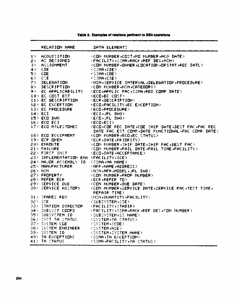
Table 2. Examples of relations ped1no t to DIN operations
RELATION NAME DRTA ELEMENTS
1 ) ACOU I S I T ION -1:014 NUMBER rCOST +PO fiLiMBER +ACC, DATE,-^) A^ DESIGNED 1:FACILIT'Y+=: MFrRACM'+REF DES +non)3) AS I GNMENT (,CON NLIMBER +OIJNER +LOC.RT I OP; +OF'S TRT oR.EC: DATC )4) CPE i"_,MRPCDE)c) COE (' '.MA•COE6) 111 * E (vrMA+CSE)( DLEGATION <N•N+.SERVICE INTERVAL+DELEGATION+PROCEDURE)8) DESCRIPTION i.CON Ni_1i4BER+N'tN+CFTEGORY)9) EC APPL I ►=ABILITY i EC L1 +AF'PL I C FAC t S.SMA rRECi COMP DATE,10) EC. COST EST (ECO ► EC COST)11) EC DESCRIPTION ^ECR+DEICRIPTION)12) EC EXCEPTION (.ECO+FAC:ILIT%'+EC EXC EPTION)13) EC PROCEDURE (.ECOPPROC•EDURE)14) ECI i'EC I+JPL DIJG)
15 ECO Dlllb i:E ►-0+•JF'L D616)16 ECO EC I (:ECO+EC I )17.E ECO MILE:{TONE: (ECOrCOE REC DATE %COE -HIP DHTE+DE'ST FRC+FAC. REC.
DRTE FRC. EST COMP r DFTE FI_INC T I OVAL r FAC COMP DATE)18) ECO EG U I PMENT (CON NUMBER +EC O .EC :STATIJ'_ )19.1 ECF OPEN iECRrDATEoPFIORITY)21.0 ENROLITE (; ►:ON NUMBER rS: HIP DATE oSHIP FAC rL ► E:ST FAC )21) FAILURE f'CON NUMBER+FAIL DATErFAIL TIMErFACILITY)22) FIR:=T Ili_.T (.ECO+PRTE-ACCEPTANCE),^:?) IMPLEMENTATION EN ►: (FRCILITY+ICE)24) MAJOR A: ' EMBLY ID ( :_ MA r MF NAME)25*- MANUFACTURER i MFR +NRME PADDRE`:c )26) N':N .'Pi_N P MFR+MODELP.JPL DAIG)27) PROPERTY ICON NUMBER+PROP NUMBER)28) REFER EC•R is ECR +REFER TO)29) :SERVICE DUE (CON NUMBER+DUE DATE)3(Y> SERVIC.E HI::TORY <CON NUMBER+:_.ERVICE DATEr'S•.ERVICE FACrTE`T TIMEr
REPAIR TIME)1 ) :.FARE:= FrE ► ;^ is Fl 11 r ^^UFNT I T1' +FAC I L I T1'
W.''' ::.E33) ::TATION DIRECTOR i:FACILITYr7 TAD IP.
34;x =IJf..','_T COORD FRCILIT`,'+ "MMrk'ACk rFEF DE r ►"'ON NUMBER)35) BUT? _Y':5 TE'M ID _UB:=Y':S:TEM r: _ NAME)3r.i :.Y"_T TR STRTlY C_`f'_TEM+TA =.TATIJ:;):3 `_•'i'_TEM CGE TEMr:=COE)38.'! "Y:=TEM ENGINEER i':Y'=TEMrN E)
'_.`r'^ TEM ID NAME )40) TA EXCEPTION: (:_:::MA +TA E:,CEPT I ON )4 1 :! TA :S THTIJ := <.'_.: MA +FF1r I L 1 T' •r r TA _ TATIJ': i
264

Tabb 3. Bxamptss of rotations pertinent to DAN engineering chs.M, lagerne"t
RELATION NAME DATA ELEMENT
42) EC APPLICABILITY (ECOPAPPLIC FACoSSMA•REQ CC"`' DATE)4:?) EC COST EST (ECO+EC CO_T)44) EC DESCRIPTION (,EC:P.PCO .JECT + DESCPIPTICH o PEi? CnMP DOiTE)45) EC EXCEPTIONS rECO•FACILI1Y9EC EXCEPTION)46) ECO MILEST0.4E - ECO.COE REC DATE+COE :HIP IATE+DEST FAC rFAC : REC DATE+
FAC EST COMPrDATE FUNCTIONAL%FAC COMP DATE)47) EC PROCEDIWE (ECO PPROCEDURE)48) EC =r. 1J S Y;. TEM ECR 9 SUIPSY TEM )49) ECI ,EC1 r.JPL DWG)50) ECO D41G k ECOP.JPL DI,IG,51) ECO EC I ! EC O +EC I )52) ECO FOPECAST ( EC.O+E:'T DE IGN FINI: H+E'^'T FHB F11`41 :11115:3) ECO KIT (ECO+DESIGH FINI' HrFAB FINISH)54) EAR OPEN (ECR GATE+PRIORITY)55) FIRST INZT 'ECO+DATE^ACO.EPTANCE)56) REFER ECP (ECP+REFER TO)
Table 4. Examples of relations pertinent to DSN maintenanceand operation documentation
PELATION NAME DATA ELEMENTS
57) CO,^."T D000MENTP REV I'y:ION9C0: T),58) RELEASE DATE DOCUMENT * REV I_ ION •RELEASE DRTE)59) TITLE -;DOCUMENT+TITLE)
Table S. Examples of ref Aloas pertinent to the DSNprogram library
RELATION NAME DATA ELEMENT:_
60) APPLICABILITY (. PROGRAM 9SSMA)
61", PROGRAM ID
^+POGRAMrLANGUAGEgTITLE)62) RELEA=E PATE
<' PPOGPAM %PELEW"E DATE)63".4 TA STATI_IZ PROGRAM P TA 1--'
. TATLI , DATE
265

Table & Examples of relations pertinent to DON logletfas
RELATION NAME DATA ELEMENTS
64) CC:T ,N'MrCOST)65) IDENTIFICATION (HZN.MFPvMODELPPART NUMBER•NOMENCLATURE)66> LEAD TIME (W149LEAD TIME)671 LOCATICI '+ ;CON NUMSER91-OCATION)66) SERVICE DELEGATION (NSNPDELEGATI0f1)69) SOUPCE (NSN•VENDOR)70) UNIT OF ISSUE (NS,N+IS'SUE UNIT)
Table T. Examples of relations pertinent to DON worbmanshlp gnu 09
RELATION NAME DATA ELEMENTS
71) DI.CREPANCY (IN:F NUMBEP9DI1CFEPANC:Y)72) ECO INSPECTION (INSP NUMBERPECOoIN'F STATUS)73) EMP CEPT STATUS r'. EMP NUMBEP.C:EPT STATU S + C:ERT ` UFJECT')74) EOU I PMENT ID o. C ON NUMBER •MFR +MODEL .NOMENCLATUIR E • vEP I RL NUMBER)75) EQUIPMENT DbIG ICON NUMBER o JPL DWG)76) IN PELT DATE INSP NUMBER+DI'POSITION•DATE:'-77) IN:=PECTION (,'CON NUMBER+INSP DATE +LOCAT ION vINSP NUMBERPIN P TYPE)78) 'SUSI.YSTEM APPLIC (INSP N1-1MEEP.SUE'1Y: TEM)
Table 8. Examples of relations pertinent to DON subsystemstatus and assignments
PELATION NAME DM TA ELEMENT:
1: DE. r•' : MArCDE)80) I-,:0E r,.^ _,MA.COF)81) IMPLEMENTATION ENG (:FAC•ILITY+IC:E')82) MAJOR f SSEMBL Y ID 1::::;'MA vMA NAME)
E S. UP :_ Y .7 T E M • .: E )84:) :_•TATION DIRECTOR i:FFr-,ILIT `('•'.TADIP)8 5) • TEM I D ^:: ':LIB _:Y:_ TEM . S _ NAME)$i, > Y:.T TA •TPT1.1:5. ; '_'i'': TEM . TA STAT ►J:7) :' Y'S.TEM COE 'r:TEMr':C'OE)88) :"i':::TEM ENGINEER !' Y_•TEM9N':E)_'', :'r' TEM I L ('='i''STEM rSY' TEM NAME:)90 ", TA EXCEPTIONS CS SMS o Thi EXCEPTION)91' s TA _ TATL':. ^:_ ::MA +FMC. I L I TY !, TA STATL► S )
266 'itIGID4AL Y X61E 1^
OF Pool,QUA

Table 0. tlxamples of relations pertinent to JPL propwy oontrol
PELATION NAME DATA ELEMENT;
?:: , ACQU I S I T I ON , PROF NUMBEF .COST +AC Q LATE 9PO NUMBER)9 .3) EMP FE: PON _ I B I L I TY ( PROP NUMBEF . EMP NL ►MBER )94 , EMPLOYEE ORG (EMP NUMBEF.EMF ORGANIZATION)9S; ECUIP SERIAL (PROP NUMBEF91•ERIAL NUMBER)96) EQUIPMENT ID e PPOP NUMBEF .MFF.MODEL +t4CMENCLI'+TURE97) LOCATION (PROP NUMBEP ►LOCATION)
Table 10. Exempts of relations pertinent to the management of automatic data processing equipment
RELATION NAME DATA ELEMENTS
98) ALP PLAN < ADP I D +PO NUMBER)99) LOCATION 'PO NUMBER+PROP NUMBEF+MFRoMODEL+LOCFTION)
267

DSN Progreoe ReW 42-44
January and February 1978
N78=24242
A New, Nearly Free, Clock Synchronization TechniqueW. H. I lietzke
DSN Operations Section
A new, near real-time, method for intercomplex clr. i, synchronization is proposed.The method consists of transmitting a symmetric frequency ramp to a spacecraft anddetermining the time at which the received ramp (in doppler residuals) occurs atoverlapping stations. Adjusted preliminary data suggest that the accuracy of the methodmay be better than 0.7 microseconds. The method requires no additional hardware andcart be done during nonnal tracks. Other, perhaps more accurate, variations of themethod are under investigation.
I. Introduction
Interstation clock synchronization is extremely importantin both spacecraft navigation and in the ultimate accuracy ofscientific data obtained from the spacecraft. Several methodsof clock synchronization are either in use or have been pro-posed. Most precise methods utilize radio signals from extra-terrestrial objects — either originating there (Very Long Base-line Interferometry) or bounced from them (Moon Bounce).There are several contributors to the ultimate accuracy of thesynchronization which all such methods have in common.These are: 1) station location uncertainty, 2) atmosphericdelays, and 3) electronic (station) delays. The new methodproposed below is no exception. These three factors, however,can be measured to an accuracy which translates to less than10 ns synchronization uncertainty.
Currently the DSN synchronizes its clocks via the "MoonBounce" method. The ultimate accuracy of this method isapproximately 5 microseconds. This system requires additionalantennas and related hardware, an operator at each site, thegeneration of special "Moon Bounce" predicts, and the datamust be collected and reduced. The method proposed below
can accomplish clock synchronization to a similar (and evenbetter) accuracy, using existing data outputs — but it does notrequire special antennas, predicts, or additional operators.Also, real-time programs can be written to compute certainparameters which will reduce analysis time and give ultimatelynear-real-time synchronization. A variation of the method canalso be utilized for Very Long Baseline Interferometry (VLBI)clock synchronization. This will be discussed later.
11. Description of Method
The method consists of transmitting a symmetric sawtoothfrequency ramp to a spacecraft. This ramp can be identical tothose currently employed for Pioneer ramp ranging. The trans-mit time should be such that the ramp is received approxi-mately in the middle of the overlap interval of two DSS whoseclock off-sets are to be determined Both DSS must be lockedto the signal throughout the duration of the ramp.
The ramp, unmodeled in predicts, will appear inverted inthe doppler residuals. This will be the data base for thesynchronization. Doppler residuals are computed by the Real
268
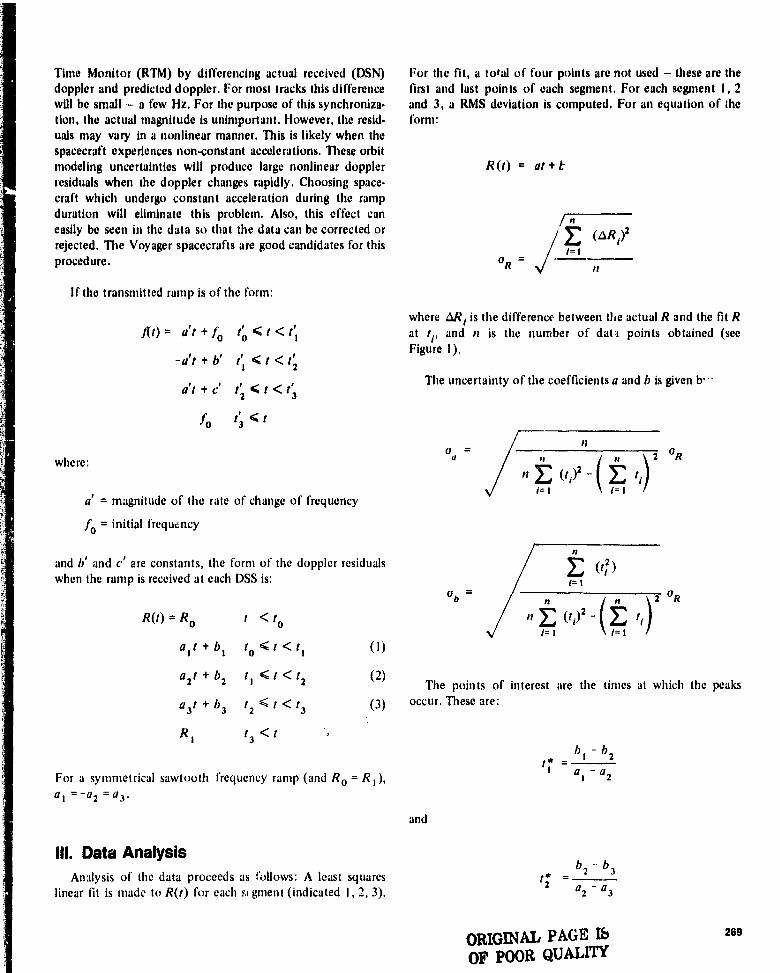
For the fit, a to tal of four points are not used — these are thefirst and last points of each segment. For each segment I, 2and 3, a RMS deviation is computed. For an equation of theform:
Time Monitor (RTM) by differencing actual received (USN)doppler and predicted doppler. For most tracks this differencewill be small — a few Hz. For the purpose of this synchroniza-tion, the actual magnitude is unimportant. However, the resid-uals may vary in a nonlinear manner. This is likely when thespacecraft experiences non-constant accelerations. These orbitmodeling uncertainties will produce large nonlinear dopplerresiduals when the doppler changes rapidly. Choosing space-craft which undergo constant acceleration during the rampduration will eliminate this problem. Also, this effect caneasily be seen in the data so that the data can be corrected orrejected. The Voyager spacecrafts are good candidates for thisprocedure.
If the transmitted ramp is of the form:
J(t) = d r + Jo to < t < t,
-dt+b' t^ 6t<tz
a't + c' t2 6 t < t3
fo t3 < t
where:
a' = magnitude of the rate of change of frequency
f = initial frequency
and b' and c' are constants, the form of the doppler residualswhen the ramp is received at each DSS is:
R(t) = Ro t < to
a l t+b lto <t<t i(1)
al t + b2 t I < t < t2 (2)
a 3 t + b3 t2 < t < t 3 (3)
R I t3 < t
For a symmetrical sawtooth frequency ramp (and R o = R I ),a 1 = _
a2 = a3.
and
R(t) = at+t
_ nas n n 12 OR
!- 1 ! I
t* = bl
b2
1 a1 - a2
!= IOR
i
where AR, is the difference between the actual R and the fit Rat t! , and n is the number of data points obtained (seeFigure 1).
The uncertainty of the coefficients a and b is given b•••
(t2 )
Qb
n( n
2 OR
r- I != I
The points of interest are the times at which the peaksoccur. These are:
Ill. Data AnalysisAnalysis of the data proceeds as ''ollows: A least squares
linear fit is made to R(t) for each si gment (indicated I, 2, 3).
t* _ b2 " b3z a2 - a3
ORIGINAL PAGE Ib 269
OF POOR QUALITY

The accuracy with which these times are known is given by
o _ (°2 +02 1 2
r l bIb2 a l - a2
_2+ b2 I
(
02 +
02 )1/2
(a ► - a2)2 a
n2
and a similar equation for orz. The equation can be put in aform containing OR and it (the number of data points for eachsegment) by approximating the sums in the oQ and obequations by integrals
^1► -+ ftdt; Etr _ft2dt.
The result -- for a sawtooth frequency ramp with a 20 minuteperiod — is:
°R 3.67 2°r l (a, - a 2 ) it /2 11
(b, - 62
aI - a2
As can be seen from the equation, a large slope will reducethe uncertainty in ti. Thus, using X-band will improve theaccuracy of t* by a factor of about 4.8 over S-band. Althoughchoosing large it (short sample times) will increase the ORsomewhat, since °; is proportional to n- 1/2, large it reducethe uncertainty of t* (approximately as n- 0.2 ). For example,1 second data will reduce the uncertainty in t* by a factor ofabout 1.6 over 10 second data.
For large t ► , the uncertainty in t* is approximately:
2.45 ;b I - b 2 I
° ► 1 (a ► - a2)2 n1/2 °R
2 1/2
+ (2.45)2
Thus, minitnizing bt is also important. No attempt was madebelow to minimize b ► , b 2 or It but this is easily done.
I have gone through this analysis using ramp ranging datafor Pioneer 10, taken at DSS 14 on DOY 209 (1977). Theexciter VCO was increased at a rate of 2.083 Hz/sec. (This ratecan be increased somewhat in future tests, without fear oflosing lock on the ramp's return.) The received S-band slope is
2201 X 48 X 2.083) + Co ^5 108.6.
The constant Co is a term involving the spacecraft motion. Theresults of the analysis are shown in Table 1, below, for 10second data, and Table 2 shows the uncertainty of the time ofthe peaks.
For this day, the "Doppler Noise" (computed for 60second data) was 0.007. This is high, noise levels of 0.003 arethe rule and values slightly tower can be obtained using aHydrogen maser. Titus, an improvement by a factor of 2 isexpe,;ttd for °; for standard data. This translates tospecification of the event (the peak) to 0 X49 ps at each station(1 second X-band data) resulting in a clock offset measure-ment accuracy of 0.7 ps (excluding other correction
uncertainties).
All of the above calculations may be incorporated into theRTM - including a check of the doppler residuals to auto-matically activate the subroutine when a ramp occurs. Whatremains then is to apply corrections to the measured clockoffset for I) the difference in signal path length (divided byC), 2) the difference in electronic delays, and 3) the differencein atmospheric delays.
As mentioned previously, this method is compatible withVLBl. Several schemes call used to correlate the data, andthese are under investigation.
The advantage of this system will be a reduction of dataprocessing time with considerable cost savings rather than animprovement of accuracy over the currently proposed VLBIclock sync method. This is possible because the spacecraft canbe considered a coherent point source - thus, circumventingsome correlation problems associated with the transversecoherence length of stellar radio sources. (This will allowsimilar accuracies with less data.) The signal level will be highand the time change of the frequency call computed beforethe fact. This last point will allow the use of more narrowreceiver bandwidths, driven by prograi. -liable local oscillators.
270

Table 1. Ton second data
Region a i (Ilz/Sec) b i Olz) aR (X t0-3 a (X 10-6) ab (X 10-4
1 -108.60002 329.0453 7.59 5.06 0.835
2 108.60002 -65484.6439 9.61 0.436 4.71
3 -108.60002 130636,9870 10.02 6.68 70.4
Table 2. Uncertainty of the time of the peaks
Peak ,i f* ( 10 sec. S-band) 0: (1 sec. S-band) a t* (I sec. X-band)
t t 7.42 ms 4.67 jAs 0.97 us
2 33.8 )AS 21.3 µs 4.4 µss
ORIGINAL PAGH 18nr POOR QUALM
271

DOPPLER RESIDUALS FORSTANDARD TRACK
R(t) _._.. __....._...._..... , _.. _..._._.._..
f
pet)1 I . r^•^^... .., ..
f
DOPPLER RESIDUALSFOR RECEIVED RAMP
♦^°3
R(t)°2
/ f
^2f = 0 (FOR FIT)
FIT TO DATA WITHPARAMETERS SHOWNFOR EACH REGION
Fig. t. Typical doppler residual plots
272

DSN Progress Report 42.44
January and February 1978
N178-24243
Tracking Operations During the Voyager 2 Launch PhaseJ. A. Wackley and G, L. Spradlin
DSN Operations Section
Tine Voyager 2 launch phase tracking operational procedures were carefully studiedand consenatively designed to accommodate an y launch contingency. This launch phasewas marked b y the first use of the Goldstone complex, including the 64 ureter antenna, astine initial acquisition location. The following report details the pre-launch planning forand subsequent analysis of'tracking operations during the Voyager 2 launch phase.
I. IntroductionOn August 20, 1977 at 14:29:44,27 Greenwich Mean Time
(GMT), Voyager 2 lifted off' from the Kennedy Space Center
signaling the somewhat unsure start of the Voyager mission.
The purpose of this mission is to study the regions of Jupiter,
Saturn, and possibly Uranus, as well as the interplanetary
media.
To begin this investigation, Voyager 2 was launched at an
azimuth of 124.09 degrees aboard a Titan 3E/Centaur DI Tlaunch vehicle with insertion into the trans-Jupiter orbit
occurring over Southeast Asia. The geometry of the parking
orbit and subsequent Jupiter transfer orbit was such that the
Goldstone Deep Space Communications Complex, specifically
Deep Space Station (DSS) 12, became the prime initial
acquisition station. This launch marked the first use of a
Goldstone station for the initial acquisition as well as the first
use of a 64 meter station during the initial pass.
This report details the pre-launch planning for the initial
acquisition pass and presents an analysis of the events of that
pass.
II. Trajectory ConsiderationsThe open window launch trajectory for 20 August pre-
sented angle and frequency rates which were comparable to
other recent parking orbit ascent launches (Ref. 1). Specifi-
cally, these rates were:
Hour Angle (HA) = -0.049 degrees/second
One Way Doppler (D1) = +82.6 Hz/second
X n -• 68 Hz/second (S-Band)
The trajectory for Voyager 2 also had the following
characteristics:
(1) Tile am ie and frequency rates were highest at open
window of any particular launch date
(2) Th.: highest maximum elevation angle was achieved for
open window launch
(3) The declination of the spacecraft was very high (410)
and would remain so for many weeks after launch
273

Of tl%. ^e three items, only the high declination angle requiredsper. , tl planning which is detailed in Section VII.
Figure I stereographically illustrates the initial pass overDSS 12 while Figure 2 depicts the elevation angle during thispass. Additionally, Figure 2 serves as a timeline for significanttracking events that occurred during the pass.
An important facet in the design of an initial acquisitionstrategy is the effect of an anorninal launch in the spacecrafttrajectory. To this end, 3a launch trajectories were providedby the Voyager Navigation team. Examination of thesetrajectories yielded the following 3o uncertainties in thetracking parameters at the rise of DSS 12:
3a Hour Angle = 0.31 degrees
3a DI = 3001Iz (S-Band)
3o D2 = 600 Hz (S-Band)
3a XA = 182 liz (S-Band)
These figures are somewhat smaller than those encountered itother recent launch phases. For example, for the Helios 2launch (Ref. 2) th° 3a uncertainties were:
3a Hour Angle = 1.15 degrees
3a DI = 3500 liz (S-Band)
3a XA = 1632 Hz (S-Band)
These data were, however, somewhat incomplete in that thereexist many different possibilities for non-standard trajectorieswhich could result in (possibly) larger errors. In light of thisand in order to insure complete success, the initial acquisitionstrategy was developed from air conservativeapproach.
111. Tracking Subsystem Software
This launch, unlike any other launch, was to be supportedusing a plethora of newly implemented software as well asmuch new hardware. Since the last (Helios 2) launch, newAntenna Pointing Subsystem (APS) and Planetary RangingAssembly (PRA) software had been implemented, the trackingprediction software had been extensively changed, the MetricData Assemble (MDA) and its associated software had beennewly implemented and the Block III Network SupportController (NSC) had come into use. As this software andequipment underwent extensive pre-launch testing, many flawsand failures were discovered, in fact, every one of the abovementioned components underwent some degree of modifica-tion during the last few months before launch.
A. Tracking Predictions
In Mardi of 1977, the DSN tracking prediction system wascompletely changed. The previous system relied wholly ontopocentric trajectory data in the form of a polynomialcoefficient tape (PCT) generated by the project navigationteam. This PCT was then evaluated by the PREDIK softwareto produce tracking predictions.
The new (and currently used) aystem requires as input aprobe ephemeris tape (PET) containing the probe trajectory interms of a central body. The PET then becomes the input tothe Fast Phi-factor Generator Program ( FPGP) which trans-lates these data t ,h topocentric observables and generates thePCT input to PREDIK.
[if course of generating the many predicts sets requiredto characterize the launch trajectories, it was found that FPGPcould not quickly or accurately produce launch phase predic-tions. These problems obviously caused concern that FPGPcou l d riot be used at all during the launch phase of Voyager.To improve the running time of FPGP there were extensivechang%s to the program files. These changes resulted in theelimination of two tapes and much operator intervention. Thisstreamlining allowed the running time to be reduced signifi-cantly.
It was also discovered that FPGP tended to over fit whenthe observables were undergoing a high rate of change. Tocorrect this situation FPGP was moAned to allow user controlof the minimum span duration thereby diminishing thetendency toward overfitting.
In later testing (in fact, within three weeks of launch), itwas found that the time from launch (TFL) option did notfunction correctly. While copies of the predicts produced atJPL had the prope! time field, those received at the stationsdid not. Since this was an important launch phase predictsoption, (see Section IV) the cause of the problem (one line ofthe program had been inadvertently omitted) was quicklyisolated and corrected.
The NSC is the L5 computer used to generate and transmittracking and telemetry predictions as well as other productssuch as the sequence of events and schedule. During pre-launchtesting it was found that the NSC software used in theconstruction of transmission files would not accept theVoyager spacecraft identifiers. It was also discovered duringthe testing cycle that the Metric Data Assembly (MDA) wouldnot permit reception of a single pass of predictions. During thelaunch phase predictions are, of course, generated oil singlepass basis. Both programs were quickly modified to correctthese anomalies.
274

Thus, after a less than encouraging start, the predictionsystem was Gnally ready for launch support with less thanthree weeks to spare.
S. APS 11 Drive Tape VerificationWith the implementation of the APS 11 software in early
1976, the format of the antenna drive tape was changedthereby nullifying the drive tape verification software. Thisleft only a check sum computation for verification of the drivetape. It was believed that this method of verification waswholly inadequate for support during this critical phase. Theoriginal APS drive tape verification program was thereforequickly modified and brought into operational usage justweeks before the Voyager 2 launch.
C. Planetary Ranging AssemblyIn late May analysis of ranging data from DSS 12 revealed a
one second error in the range acquisition (To ) time as reportedby the MDS version of the Planetary Ranging Assembly (PRA)software. Like the other previously discussed problems, thisone was quickly corrected and the PRA was made ready forlaunch support.
IV. Angle Drive StrategyThe angle drive strategy for the Voyager 2 was essentially
the same strategy successfully used during previous launchesand was based upon the following considerations:
(1) It was desired that the uplink be acquired shortly afterrise,
(2) Usage of a drive tape was required during the one-wayto two-way transition,
(3) Acquisition of early (near earth) auto track data wasdesired, and
(4) It was desired to lock the receiver coupled to theS-Band Cassegrain antenna as well as the S-handAceuisiticn Aid Antenna (SAA) connected receiverprior to initiation of the uplink sweep.
It was planned that at least four and possibly live drivetapes would be generated to assure the station of the bestavailable Jrive tape. The antenna drive strategy then became:
(1) At launch minus seven days (or L-24 hours it' thelaunch date slipped) open, mid and close window drivetapes were to be generated. These tapes would be inTFL format and would be used as back ups for drivetapes to be produced during the final countdown. Touse these tapes, a time offset (At) equal to the actuallift-off time would be entered into the APS. Which tape
to use would be specified by the Tracking NetworkOperations Analyst (NOA).
(2) At L-105 minutes a new drive tape with times in GMTformat would be generated. It had been determinedpreviously that (based upon an analysis of angle rates)the SCM antenna beam width would tolerate an errorof up to three seconds in lift-off time before it wouldbecome extremely difficult to lock the receivers. TheL-105 minute predicts would then be prime if launchwas within three seconds of expected.
(3) At L4 minutes, a contingency predicts set based upona lift-off plus three second trajectory would be gener-ated. It' lift-oft' was more than three seconds late, thesepredicts would be transmitted to the station for use inpunching a drive tape.
(4) Finally, if none of the previously mentioned drive tapeswere adequate, a prediction set based oil actuallift-off time would be generated as soon as that timebecame known. A drive tape based on these predictionswould become prime.
Fallowing the uplink acquisition, as early as practicable theantenna drive mode would be changed to auto track. Thisswitch would be done in three steps: the signal on the SAAreceiver would be peaked using offsets to the latest availabledrive tape, auto track would then be accomplished on the SAA,and finally, auto track would be accomplished on the SCM.
V. Initial Uplink AcquisitionThe Voyager initial uplink acquisition had been designed
with the following criteria in mind:
(1) The uplink should be acquired at the earliest prac-ticable time based on station capabilities and spacecrafttrajectory constraints,
(2) The uplink acquisition sweep should span a frequencyrange and be at a rate that best guarantees acquisitionon the first sweep, and
(3) The uplink acquisition should be complete in time tohave all stations (particularly DSS 14) ready to receivethe critical 7.2 kbps telemetry data.
The following uncertainty information pertaining to theuplink was made available by the Voyager project:
3o Trajectory 192 1 l (S-Band)
3a Measurement 1000 1 l (S-Band)
3a Receiver "Random Walk" 2000 1 l (S-Band)
3a SAC Temperature — 1500 fix (S-Band)
275

Combining the above, one arrives at a total 3o uncertainty (1) Transmitter connected to the S-Band Acquisition midof: Antenna (SAA) and set to radiate at 10 kw.
3o Total — 2700 Ilz (S-Band)
or — 28 Hz (VCO)
This uncertainty was extremely small with respect to uncer-tainties for previous missions (for instance 3o foi Viking was5300 Hz), therefore, to be extrem, ' onservative (and henceallow for any sort of abnormal I, .,ch vehicle or spacecraftperformance) and since there was no real impact on tuningduration, the previously described 3o uncertainty was morethan tripled resulting in a sweep of approximately XA t9600 It (S- Band)or XA :t 100 Hz (VCO).
The Voyager spacecraft receiver tuning rates are boundedby:
60 Hz/sec < tuning rate < 1000 Hz/sec (S-Band)(or 0.6 Hz/sec < tuning rate < 10 Flz/sec (VCO))
under the strong signal (-100 dBm) conditions that were to beencountered during the initial pass. For the initial acquisition asweep rate of 3 Hz/sec (VCO; or 288 Hz/sec at S-Band level)was selected because:
(1) The rate was well above the push limit of the receiverand thus would result in a successful acquisition.
(2) Should it become necessary to manually tune theexcites, ii was believed that the station could notaccurately tune at a higher rate than the chosen rate.
(3) A rate of 288 Hz/sec (S-Band) would result in aneffective (Doppler rates considered) tuning rate ofapproximately 238 Hz/sec at the spacecraft receiver.This rate was very nearly the geometric mean of theupper and lower sweep rate limits (245 Hz/sec).
The sweep was to start at lift-off plus 78 minutes,approximately 5 minutes after the spacecraft would have risen.This allowed sufficient time for the necessary sideband/sidelobe searches before starting the uplink acquisition.
Finally, the sweep was to consist of a single upleg in thedirection of the change of XA, with the ending frequencybecoming the TSF for the remainder of the pass. This wasadvantageous in that no additional tuning to reduce staticphase error (SPE) would be required during the remainder ofthe pass.
Incorporating the preceding information, the general uplinkacquisition procedure was:
(2) Transmitter on at start of uplink sweep minus 20seconds.
(3) Radiometric data to be flagged two way at start ofsweep minus 10 seconds. (This would enable the NOCTto know when (and if) two-way lock was achieved andwhether lock was on the main carrier or a sideband.)
(4) Sweep to start at L+78 minutes or approximately 5minutes after spacecraft rise.
(5) Sweep to cover at least XA t 100 Hz (VCO) at a rate of3 Hr./sec (VCO).
(6) Sweep duration to be approximately 80 seconds.
If the first sweep failed a contingency sweep encompassinga region 50 percent larger (XA t 150 Hz (VCO)) than theoriginal sweep would be performed, starting 2 minutes and 30seconds after completion of the first sweep. The contingencysweep wo!dd consist of a downleg and an upleg followed by asweep back to TSF executed continuously with no pausesbetween legs. (Of course, if two-way was achieved anytimeduring the contingency sweep the station was to stop tuning,lock the receivers and then tune directly to TSF.) The tuninginstructions for both sweeps were to be provided to DSS 12w.-i) before lift-off via a sweep message similar to that shownin Fib. 3.
VI. Ranging
Range data collection for Voyager was to begin shortlyafter the initial acquisition at DSS 12. Additionally, plans weremade to transfer the uplink from DSS 12 to DSS 14 so thatranging could continue for as long as possible.
Originally, it had been planned that the ranging would bedone with eighteen component acquisitions interspersed withten component acquisitions. After the risks inherent inchanging range parameters (i.e., possibly significant losses ofdata) were pointed out to the Voyager project, it was decidedto pipeline fifteen component ranging acquisitions separatedby three differenced range versus integrated doppler (DRVID)measurements.
The following parameters were to be used:
(1) T I = 59 seconds
(2) T2 = 2 seconds
(3) T3 = 60 seconds
(4) TO= 3CCEE
276
(5) RTLT . 0 seconds
(6) Number of components a 15
(7) Carrier Suppression n 3 dB
VII. Downlink Acqulshlon at DS6 62Because of tha high declination (41 0 ) of the Voyager 2
trajectory, it was found that DSS 62 would be unable toacquire the spacecraft downlink until the spacecraft reachedan elevation of approximately 160 , this being the minimumelevation at which the antenna could be pointed at thisdeclination. On the first pass, this constraint would cause amore than fifty minute gap between the end of track at DSS44 and the start of track at DSS 62. However, because of thestrong signal levels expected during that time, it w iuld bepossible to narrow the gap considerably using the SAA. Fromavailable information, the threshold of the SAA was computedto be:
-164.4 dBm in the 48 Hz RF Bandwidth-170.4 dBm in the 12 Hz RF Bandwidth
The signal level at the time of DSS 44 set was expected tobe at least -161.4 dBm. Thus, there would be from three tonine decibels of downlink margin. From (very old!) SAAantenna patterns it was found that the angular offsets necessaryto reduce the signal level to threshold were:
^-8° for threshold in the 48 liz RF Bandwidth
— 15° for threshold in the 12 Hz RF Bandwidth
These offsets translated (assuming sidereal angle rates) to anincrease of front to 61 minutes in the view period of DSS62. Thus, the obvious conclusion was that, by judicious use ofthe receiver, the downlink could be acquired using the broad(16°) beam of the SAA and at a much lower elevation thanthat at which the main antenna could even point, therebyreducing the gap in the tracking of the spacecraft and possiblyeliminating it completely. The extended coverage is stereo.graphically illustrated in Fig. 4.
It was decided to attempt io close the downlink gap (thegap in the uplink would be tolerated) using the followingprocedure:
(1) Two sets of predicts would be generated for DSS 62.Otte set, to be used for driving the antem,.., would havethe actual horizon mask. The other set would have azero degree elevation horizon and would be used tocompute frequencies for the SAA receiver sweep.
(2) DSS 62 would drive to the specified rise point (asdefined by the antenna limits) at least by the time thatthe spacecraft would reach zero degrees elevation.
(3) At the time of the earliest possible acquisition, DSS 62personnel would slowly sweep the receiver in the 12 HzRF bandwidth and attempt to acquire the downlink.
(4) When the spacecraft reached the rise point the SCMreceiver would be locked and normal tracking, includ.ing an uplink acquisition, would begin.
The coverage gap would continue for several weeks afterlaunch but, unfortunately, this use of the SAA would berestricted to (because of signal level constraints) the first pass.
VIII. Post Launch Analysis
A. Tracking Predictions
1. Prediction Generation. Minutes before the scheduled14:25:00 GMT liftoff time the Voyager 2 countdown wentinto a hold that was to last four minutes and 44 seconds. Thisdelay made it imperative that tracking predictions based onthe actual lift-off time be generated and made available to theinitial acquisition stations prior to spacecraft rise, approxi-mately 70 minutes after launch.
Because of the suddenness with which the hold wasinitiated and terminated, there was much confusion aboutwhat the actual lift-off time was to be. This confusion resultedin the required lift-off PET being delivered approximatelyfifteen minutog after lift-off.
Thanks in large part to the pre-launch streamlining (SectionIIIA), predicts were available approximately twenty minutesbefore the expected spacecraft rise.
2. Prediction Accuracy. The accuracy of the launch phasepredictions (as measured by pseudo-residuals) was very good.The pseudo-residuals, computed in near real-time by differ-encing radiometric data with the lift-off tracking predictions inthe NOCC Tracking Real Time Monitor (RTM), had thefollowing average values during the early portions of thelaunch pass at DSS 12:
AHA -a -0.085 degrees
OD2 25 -130 Hz (S-Band)
OXA a5 8.9 Hz (VCO)
These differences may be compared to the 3a uncertaintiespresented in Sections 11 and V:
3a OHA 25 0.309 degrees
3a OD2 2- 588 liz (S-Band)
3a AXA 2! 30 I-iz (VCO)
277
As can bo seen, all residuals were well within the 3ouncertainties. The small (lour Angle residual was especiallysignificant in that it facilitated the spacecraft acquisition atDSS 14 by being less titan the beamwidth of the 64 meterantenna.
The two way doppler residual continued to increasethroughout the pass attaining a value of approximately -169Iiz (S-Band) late fit pass at DSS 12.
The value of the OXA was very small considering the manypossible sources of error, both trajectory and temperature. The3o uncertainty provided by Voyager telecom was thus shownto be very accurate.
S. Initial Downlink AcquisitionThe initial downlink acquisition at DSS 12 proceeded very
smoothly with acquisition occurring at 15:41:31 GMT orapproximately one minute before the expected spacecraft risetime, As can be seen in Figure 5, Cite receiver was sweptthrough a very wide (approximately 12 Kllz) range of fre-quencies apparently centered at the downlink frequencyexpected at spacecraft rise and commencing well beforerise.
The early acquisition is due to the fact that because of thehigh declination angle, spacecraft rise was dictated by theantenna mechanical limits (see Figure 1) rather than the localhorizon. Thus, it was possible for the SAA to "see" thespacecraft below the antenna limits. Additionally, because ofthe high signal levels present during this phase it wab possibleto lock the SCM receiver as the spacecraft passed through thesidelobes of the SCM antenna resulting fit approxi•mately 40 seconds earlier than planned.
C. Initial 'Two-Way Acquisition at D88 12Shortly after lift-off an apparent problem with the space-
craft inertial reference unit gyros was detected by the project.Because of the nature of the problem (the attitude controlcomputer had changed gyro pairs several times), projectrequested that the DSN acquire the uplink at the earliestpossible time to allow fot emergency commanding, if itbecame necessary Since the initial uplink sweep had alreadybeen designed to start at the earliest possible time (see SectionV) it was decided not to depart from the current (familiar)plan.
The uplink acquisition parameters provided to DSS 12were:
(1) Transmitter on: 15:47:40 GMT
(2) Transmitter power: 10 KW
(3) Frequency: 22014140.0 Hz (VCO)
(4) Start tuning: 15:48:00 GMT
(5) Tuning rate: 180 Hz/min (VCO)
(6) Tune to: 22014380.0 11z (VCO)
A comparison of the instructed sweep with the sweepactually perforated at DSS 12 is shown in Figure 6. As can beseen, the sweep was performed excellently and closelyfollowed the expected tuning pattern.
The spacecraft receiver was acquired at 15:48:36 GMT,within 10 seconds of the expected time.
The acquisition of the two way downlink did not,unfortunately, proceed as smoothly as that of the uplink. Thereceiver was quickly reiocked (in about 3 seconds) to thecoherent downlink. It was soon noticed that the doppler resid-uals were larger than expected (almost six times the 3o magni-tude) and changing very quickly (see Table I and Figure 7).
At 15:49:57 GMT, receiver lock was broken and a sidebandsearch performed. Upon reacquisition of the downlink thedoppler residuals showed that the receiver had again locked toa spurious signal. This time, however, the doppler residualsindicated a positive bias but with the same magnitude as thosecalculated before the sideband search. Additionally, the signalwas very noisy with doppler noise averaging more than I I Hz.
At approximately 16:00:00 GMT, DSS 12 was Instructedto perform yet another sideband search. During this search thereceiver was swept through a frequency range of approxi-mately 170 KHz (S-Band level) around the expected carrier.When the receiver was relocked at 16:00:30 GMT, the carrierwas finally acquired as indicated by a doppler residual ofapproximately -130 Hz and doppler noise of approximately0.030 Hz.
The cause of the spurious signals has not been preciselydeterntuted. H+ • never, it Is believed that since:
( I) No other station experienced the same problem
(2) The spurious signals were spaced evenly (approximately4 KHz) on both sides of the expected carrier frequency
(3) Tito station reported that they returned to the originalfrequency after the sideband search
the spurious signals may have been an artifact of the effect ofthe high signal level on the DSS 12 receiver.
278
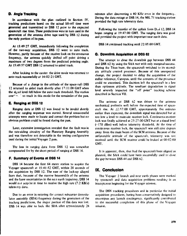
D. Angle Tracking
In accordance with the plan outlined in Section IV,tracking predictions based on the actual lift-off time weregenerated and transmitted to DSS 12 prior to the expectedspacecraft rise time. These predictions were in turn used in litegeneration of the antenna drive tape used by DSS 12 duringthe early portion of its pass.
At 15:49 :27 GMT, immediately following the completionof the two-way acquisition, DSS 12 went to auto track.However, partly because of the receiver lock on the erroneousfrequency, the antenna quickly drifted off point driving amaximum of two degrees from the predicted pointing angle.At 15:49:57 GMT DSS 12 returned to aided track.
After locking to the carrier. the drive mode was returned toauto track successfully at 16:02:21 GMT.
Because of a change in the attitude of the spacecraft DSS12 returned to aided track shortly after 17:11:00 GMT whenthe s16.0 level fell below the auto track threshold. The stationcont' - ' to track in this mode for the remainder of the pass.
E. Ranging at OSS 12
Ranging data at DSS 12 was found to be invalid shortlyafter the ranging sequence was started. Several unsuccessfulattempts were made to locate and correct the problem but noobvious problem could be found during the pass.
Later, extensive investigation revealed that the fault was inthe rate-aiding circuitry of the Planetary Ranging Assemblyand was therefore not detectable in the testing configurationused during the initial Voyager 2 pass.
The loss in ranging data front DSS 12 was somewhatcompensated for by the short period of ranging at DSS 14,
F. Summary of Events at DSS 14DSS 14 became ttte first 64 meter station to acquire the
Voyager spacecraft at 15:41:52 GMT, within 20 seconds ofthe acquisition by DSS 12. The case of the lock-up allayedfears that, because of the narrow bearnwidth of the antennaand the laree uncertainties in the necr earth trajectory, DSS 14would not acquire fit to receive the high rate (7.2 KB/s)telent try data.
Due to an error in entering the correct subcarrier demodu.lator assembly (SDA) frequency during the generation of thetracking predictions, the major portion of this data was lost.DSS 14 was able to lock the SUA after arnroxintately 28
minutes after discovering a 40 Atli error in the frequency.During tine data outage at DSS 14, the Mil. 71 trucking stationprovided the high rate telemetry data.
Following the transfer of tine uplink from D:..; 12, DSS 14began ranging at 19:47:00 GMT. 'The ranging data was goodmid provided the project with important near oath data.
DSS 14 continued tracking until 22:05:00 GMT.
®. Downlink Acquisition at DSS 62The attempt to close tine downlink gap between DSS 44
and DSS 62 by using the SAA met with only marginal success.During the Titan burn, the spacecraft switched to its second•ary attitude control processor. Because of this unexpectedchange, the project decided to delay the acquisition of thestellar reference, Canopus, until the contents of the processorcould oe examined. This decision left the spacecraft in a lessthan optimum attitude. The resultant degradation in signallevel severely impacted the "off point" tracking sche ►nedescribed in Section VII.
The antenna at DSS 62 was driven to the antennamechanical prelinnits well before the expected time of space-craft rise. At 12:57:00 GMT, approxhnately five minutesearlier than expected, the downlink signal was detected but attoo low a level to nnainwin receiver lock. Continuous receiverlock was finally achieved at 23:27:00 GMT but at a sigtial level(-170 dDnt) well below telemetry threshold. At the time ofcontinuous receiver lock, the spacecraft was still nine degreesaway front the main beans of the SCM antenna. Because of theunfavorable attitude of the spacecraft, telemetry was notreceived until the SCM receiver could be locked at 00:02:00GMT.
It is apparent, then, that had the spacecraft been aligned asplanned, the SAA could have been successfully used to closethe gap between DSS 44 and DSS 62.
IX. ConclusionThe Voyager 2 launch and near earth phases were marked
by spacecraft and data acquisition problems resulting in aninauspicious beginning for the Voyager mission.
The DSN tracking procedures and in particular the initialacquisition procedures, having been conservatively designed toencompass any launch contingency, significantly contributedto the successful completion of this phase of the Voyagermission.
279

References
1. Berman, A.L. and J.A. Wackley, "Tracking Operations During the Viking I LaunchPhase," in The Deep Space Network Progress Report, 42 .30, pp. 273 .290, JetPropulsion Laboratory, Pasadena, Calif., December 15, 1975.
2. Bright, L.E., "Tracking Operations During the Hellos 2 Launch Phase," in The DeepSpace Network Progress Report, 42 .32, pp. 277.295, Jet Propulsion Laboratory,Pasadena, Calif., April 15, 1976.
280
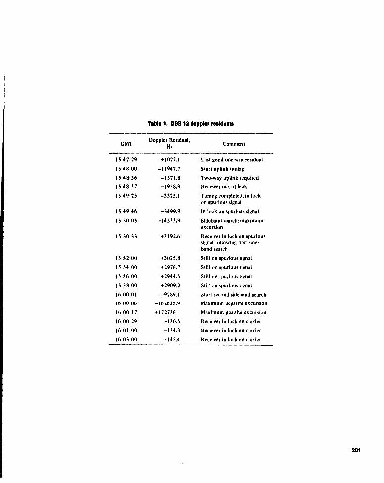
Table 1. 098 12 doppler residuals
Doppler Residual,GMT Hz Comment
15:47:29 +1077.1 Last good one-way residual
15:48:00 —11947.7 Start uplink tuning
15:48:36 —1571.8 Two-way uplink acquired
15:48:37 —1958.9 Receiver out of lock
15:49:25 —3325.1 Tuning completed; in lockon spurious signal
15:49:46 —3499.9 In lock on spurious signal
15:50:05 —14533.9 Sideband search; maximumexcursion
15:50:33 +3192.6 Receiver in lock on spurioussignal following first side-band search
15:52:00 +3025.8 Still on spurious signal
15:54:00 +2976.7 Still on spurious signal
15:56:00 +2944.5 Still on -purious signal
15:58:00 +2909.2 Still on spurious signal
16:00:01 —9789.1 Start second sideband search
16:00:06 —162635.9 Maximum negative excursion
16:00:17 +172736 Maximum positive excursion
16:00:29 —130.5 Receiver in lock on carrier
16:01:00 —134.3 Receiver in lock on carrier
16:03:00 —145.4 Receiver in lock on carrier
281
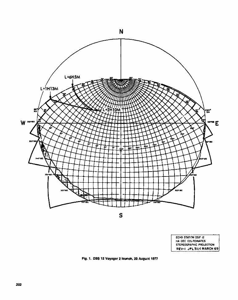
W `E
N
S
ECHO STATIIN DSIF 12HA-DEC CO(RDINATESSTEREOGRAPHIC PROJECTIONREV-1 JPL3114 MARCH 69
Fig. 1. DSS 12 Voyager 2 launch, 20 August 1977
282

00
AD
tvig is if
I 'd ce)
5c--RANGE mOD OFF
^mo'A^;17')9 34RANGING BAD FECEI /Ep
16 10- or, 01-T OF LOCKIT{31i 72
ALJOTRACK R;^E CC--- I V- U
'-CC r
16-1,24417 19 2-EE
CAk;;.j E ? ACCURE0SiDESAND SEAPCH 02 16 00- 303016
is
RA-4,GING BAD
I a 41-%
FANGE MOD OFF"IE 42-26
TAPE MYA15 SG 1C SiD£z^ SEARCH •I
3C
NRAGE h&00 of"Ak;Tr-rRACK15 49 4j
2c rmO-"A ACoujpED LOCKED ON SPUPICruS SIGNAL
t,
Z ---15-4P 36 IS48 39,
O
TRA JTTENS"R Of.47 t.',
T-PANSFFP TO
DSS 141945.02
SFACUCUFT SET210- 341le
L ;D --.. OF SsrN^L20- i; le
slnEL15aE LOCKT5 4: 1'.
;'Ecr I 11FE; I ra LOCK,SPACECRAFT PISE
e-1 31
15-00 11- or, 17 OG i a-00 19 orj 2r- Tj 21 -00
GAT 21. AJC-4-57 17-7
Fig. 2- SpWea-aft elevation at OW 12, V"MW 2 btoUh
poco
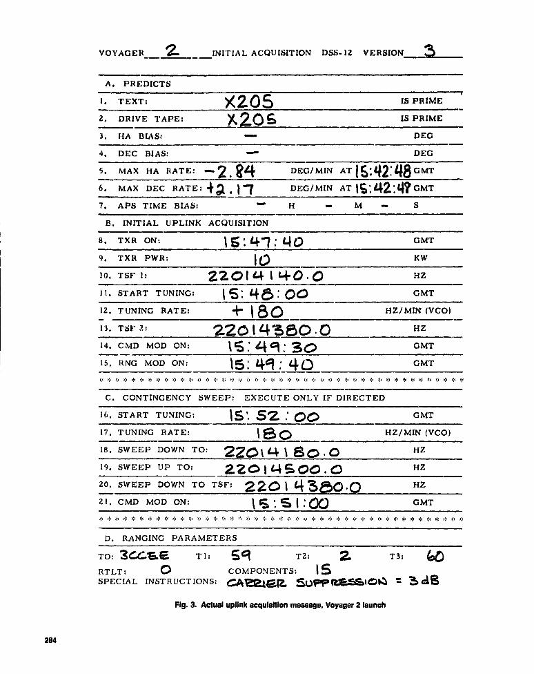
VOYAGER__ 2'INITIAL ACQUISITION DSS•12 VERSION 3_
A. PREDICTS
I. TEXT: X205 IS PRIME
2. DRIVE TAPE: X 2-O 5 IS PRIME
3. HA BIAS: DEC
4. DEC BIAS: DEG
5. MAX HA RATE: - 2. DEC / MIN AT 16:42:48 GMT
6. MAX DEC RATE: +a - 1 ^ DEG/MIN AT 15;f.^2;L^^GMT
7. APS TIME BIAS: "" H M -- S
B. INITIAL UPLINK ACQUISITION
8. TXR ON: ' S. 47: L4 0 GMT
9. TXR PWR: 1 0 KW
10. TSF 1: 220 1 4 1 40 . 0 HZ
11. START TUNING: 1 15 : '48: 00 GMT
12. TUNING RATE: + I aO HZ/MIN (VCO)
13. TSF Z: 2201 4S50 -0 HZ14. C MD MOD ON: IS: 4^ 9 : 30 GMT
15. RNG MOD ON: ' S : 419: 4 Q GMT
r:c >',: * , * * * >;^ 0.1 e4 >;< r',i r >;: :;t , >'a ..°,a $s Y,: tt , >.' >" do qr is >•c, e" i^' e., $" Y" * ^"
C. CONTINGENCY SWEEP: EXECUTE ONLY IF DIRECTED
16. START TUNING: IS , 52 : O0 GMT
17. TUNING RATE: 0 HZ/MIN (VCO)
18. SWEEP DOWN TO: 22014180.0 HZ
19. SWEEP UP TO: 220 I (4 Cam. OO - Q HZ
20. SWEEP DOWN TO TSF: 2-20 1 '4 `' SCE ,U HZ
21. CMD MOD ON: { 5 S ( GMT
:F * ;4 ':' >:: * >,, $a e,, ':' o:: is .:: Y,; o; >^: r:< o:: a r:^ >:a Y,c ., $a >4 gt ;4 ^k Y,t $a Y,a ^t >;a oV
D. RANGING PARAMETERS
TO: U4S66. T l:
RTLT: 0SPECIAL INSTRUCTIONS:
S q T2: 2
COMPONENTS: 5CAMSM SuPp-.SIOIJ
T3:
= d^
Fig. 3. Actual uplink acquisition message, Voyager 2 launch
284

Nswat apt
Na42
EXPECTED SAARECEIVER LOCK23:02:30
;.,.-ANTENNAFINAL LIMIT
!:
,
n• ntc
^to•.1
^1n•e!'1
,eo • nrc I
I
190-42 180-42
S
CEBREROUS STATION OSIF 62MA—DEC AND AZ — EL COORDINATESSTEREOGRAPMIC PROJECTION
JPL 3151 SEPT 67
Fig. 4. OSS 62 Voyager 2 launch, 21 August 1977
ORIGINAL PAGE Ib
DID' POOR QUALITY 28S

NCCa)
12000 --_^_.. _— — - -- ^ _ _ _ -_-T---r^__^
10000 -- --- .^-I
I
98000
96000 ---^----^ •
x94094000 - — ^• Y_ • •
z__—. _—T . - • -----
x . •
Z 92000 • ! • i• SPACECRAFT RISE (PREDICTED)O • • •
•15:42:36
w i }••+a 90000 __
o • j
3 •• RECEIVER IN LOCK(SCM)Z88000 - • - ------ ^.__ ----- -------- 15:41:57O •• •
•
• RECEIVER IN LOCK (SAA)86000 --_ +_ ---= - L 15:41:31
PREDICTED IWAY DOPPLER
-__ONE !84000 ---- - _. +- ------ --.I - --
82000i
1540 30 15:41:00 15:41-30 15:42700 15:42:30 15:43:00GMT
Fig. S. Initial domfink acquisition at DW 12, VayaW 2 launch
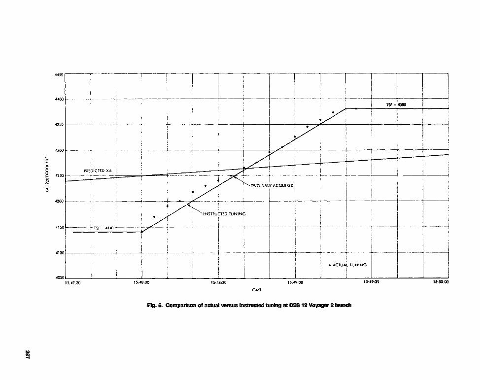
15:47:30 15:48:00 15-48:30 1549-00 15-49:30 15-5Q:00
4450
4400
4350
4300
4250
4200
4150
4100
4050
GMT
Fig. 6. Comparison of actual versus instructed turdng at DSS 12 Voyager 2 launch
NCIA4
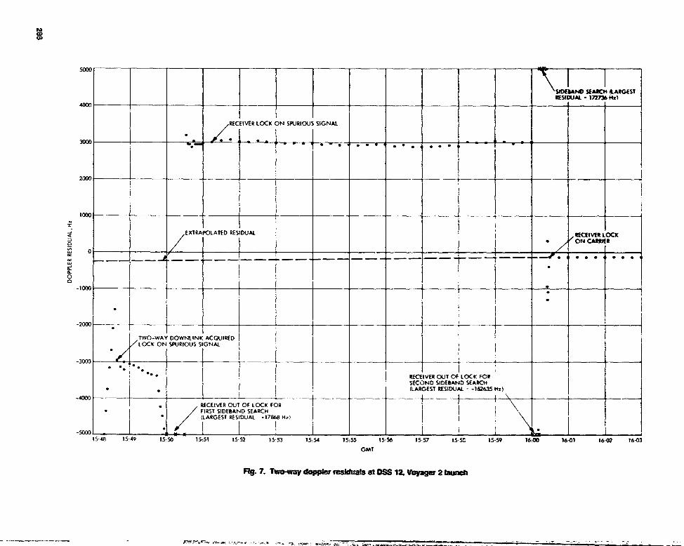
NCDco
15:55 15:56 15757 15-Z 15.59 16:00 16:01 16:02 16-03GMT
Rg. 7. Two-way dOPPW fftWkAllb at WS 12. VoyaW 2 bunch
1000xa0N
Q
J6dOin
-1000
-4000
-3000
-2000
-500015:d8 15:49 15:50 15:51 1552 15:53 1554
400(
200(
500(
300(
SIDAAIm SEARCH {LARGESTRESIDUAL = 172796 Hz)
•
RECEIVER1
LOCK ON SPURIOUSi
SIGNAL
EXTRAPOLATED RESIDUAL RECEIVER LOCK• ON CARRIER
•
•••
•TWO-WAYLOCK ON
DOWNLINKSPURIOUS SIGNAL
ACQUIREDj
1 i
iRECEIVER OUT OF LOCK FORiSECOND SIDEBAND SEARCH
• • (LARGEST RESIDUAL - -162635 Hz)li
•• RECEIVER OUT OF LOCK FOR
/ FIRST SEARCHI(LARGEST
EST US DUAL -17868 Hz)
1 ; I

DSN Prglraaa ROW 42.44 January and F"ary 1978
"'79-2 4244
An Effective Procurement and FinancialManagement Reporting System
J. B. Rozek and F. R. MaioccoDeep Space Network Support Section
This article describes the existing computerized Goldstone Procurement and Financial(GPF) management data base system. Sample management analysis reports are includedand discussed along with estimated cost swings and anticipated benefits of the computer-lzed system. In general, the system structure and procedures contained In this article arerelevant to any company's financial and procurement data acquisition and informationhandling system. Test data are used throughout this report to demonstrate the capabilityof tht GPF system of programs.
I. IntroductionThe general view of the existing computerized GPF Data
Management System is shown in Fig. I and discussed inRef. (1). Figure I briefly indicates that the GPF user has thecapability to input pertinent data to the data base and receivevarious GPF reports via a remote computer terminal. Allinformation handling, updating, sorting, searching of files,storage and report generation is performed by the computer.The table, report, and figure numbers noted in Fig. I pertainto the respective items in this article.
Several major files are required to accommodate the GPFdata and to provide the essential statistics for a requestedmanagement report. The pertinent files are a Purchase File,Cost Center File (COC), Budget File, Vendor File, JPL File,Stock Issue File (SIS) and Disbursement File (DISB). Therecord structure of these respective flies are shown in Tables Ito 7 and sample computer status codes for Purchase Requisi-tions (PR) an y_' Purchase Orders (PO) are listed irk Table 8.
The developed system of programs (file generator, updatingand report writers) is user oriented. Prompting information forthe user is available to minimize development of an extensiveuser training program and permits front-end editing to improvedata base integrity.
The subsequent sections of this article discuss the manage-ment application programs. Initially nine application programswere developed for monitoring procurement and financial mat-ters at Goldstone; and they are:
(1) GDSCC Procurement Accomplishment Report:
Part 1: Purchase Requisition ReportPart 11: Purchase Order Report.
(2) Commitment Category Summary Report.
(3) Business Subcontracting Report:
Part I: Small Business ReportPart ll: Large Business Report.
289

(4) Purchase Requisition Status Report.
(5) Monthly Specified Account Report.
(6) Monthly Specified Cost Center Report.
(7) Specified Account Budget Report.
(8) Specified Cost Center Budget Report.
(9) An All Account Budget Report.
These report programs satisfy the requirements of Ref. (1),and utilization of these reports by the managers/users insuresthat they will gain better visibility in procurement and finan-cial matters of their particular cost center, account, and/orbudget.
Description of Report Writer ProgramsThe first four reports noted above essentially are workload
related and sununarize the activity performed by the GPFgroup during a particular reporting period. The remaining fivereports (numbers 5 through 9) are financial type reports inthat monies are related to specific accounts, cost centers, andbudgets.
A. The GDSCC Procurement AccomplishmentReport
This two-part report contains PR and PO information inreference to PRs received, outstanding PRs. POs processed andoutstanding POs for any specified period of time.
The following detail information is provided to the user forthe specified reporting period.
1. Part l: Purchase Requisition Report (Fig. 2).
(1) The total number of PRs received in a given monthwith further breakdown by PR Number and Status(routine, urgent, etc.)
(2) The total number of outstanding PRs with furtherbreakdown by PR number and Status (routine, urgent,etc.)
(3) The committed dollar value per outstanding PR
PRs that have committed dollar values of $0.00 indi-cate° as a minimum that the PR is either cancelled orthe received PR became a PO or at the time of dataentry the dollar value of the outstanding PR wasunknown.
(4) The total committed dollar value.
This report briefly informs the user of input trans-actions to the GPF unit and identifies additional work-
loud for both the procuring agent and the data entryclerk. A cursory view of Fig. 2 informs the user, forexample, that three urgent Pits are outstanding andeight outstanding Pits were written prior to the report•ing period under investigation. Should an outstandingPR have no dollar value listed, further investigatic. ► bythe user is required in order to determine the accuracyof the estimated total committed dollar value. Manage-ment inay view that a significant number of outstand.ing PRs indicate potential problems in workload, per-sonnel or training, and thus institute policies andprocedures to improve organizational efficiency.
2. Part II: Purchase Order Report (Figs. 3 and 4).
a. Purchase orders released (1,1g. 3). This part of the reportidentifies the total number of I'Os written in a given month. hhighlights a ft!rther subcategorization by status to five (5)classes of Purchase Orders per management's request (Routine,Urgent, Blanket Contract, Subcontract, and Petty Cash). Itidentifies a portion of the procuring agent's work load, theindividual dollar value per 110 and the total dollar value han.died per reporting period.
b. Outstanding Purchase orders (Fig. 4). This portion of thereport identifies the total number of outstanding POs perreporting period, the identical subcategorization by status asdescribed above, the individual dollar value per PO and thetotal obligated dollar value per reporting period.
The buyer should follow up on POs where dollar values aremissing in order to insure proper data base updating. This isessential for accurate financial reports.
Reviewing Figs. 2 and 3, the manager/user can assess theGPF work unit's efficiency by creating an efficiency ratio(outputs to inputs), i.e., POs processed to PRs received oroutstanding. A closer review of Figs. 3 and 4 indicates thatthree (3) Purchase Orders (222222. 338620, 888888) werewritten in March '76 and closed out. Therefore they do notappear on the outstanding PO report.
S. The Commitment Category SummeryReport (Fig. S)
This report contains procurement commitments in variousdollar value categories. The following detail information isprovided to the user:
(1) The number and dollar value of transactions valuedfrom $0 — 500.
(2) The number and dollar value of transactions valuedfrom $501 — 1,000.
290

(3) The number and dollar value of transactions valued 2. Port 11: Large Husinesis Subcontracting Repor t (Fig. 7).from $1,001 2,500.
(4) The 110 number, PO date, Vendor name and dollar a. Contracts under $10,000. The number of contracts and
value of the respective contract valued from $2,501 r total dollar value under $10,000 awarded to large businesses
10,000,
with a further breakdown by Purchase Order number, Vendorname and the respective dollar an ►ount are identified.
(5) The W number, PO date, Vendor name and dollarvalue of the respective contract valued from $10,00125,000.
(6) The PO number, PO date, Vendor nano and dollarvalue of the respective contract valued from $15,001100,000.
(7) The 110 number, PO date, Vendor name and dollarvalue of the respective contract valued over $100,000,
(8) The total obligated dollar value per reporting period,
The sample printout also indicates to the user that thereexists in the data base possible erroneous vendor codes forcertain PO numbers. This part of the printout is an editing clueto the user that either (1)the Vendor file must be updated toinclude the noted vendor codes or (') the vendor cod_ for theparticular PO number identified must be corrected. lienceonce these corrections are made an accurate report can then berecreated.
C. The Business Subcontracting Report(Figs. 8 and 9)
This two-part report reflects the number of contracts andtheir dollar value above and below +10,000 with respect tolarge and small businesses. The category of a business, large orsmall, is determined before data is entered into the VendorFile (see Table 4). This report satisfies a NASA requirementfor the GDSCC Contractor.
The following information is provided to the user
1. Part I: Small Business Subcontracting Report (Fig. 6).
a. Contacts tinder $10,000. The number of contracts andtotal dollar value under $10,000 awarded to small businesseswith a further breakdown by Purchase Order number. Vendorname and the respective dollar amount are identified.
6. Contracts carer $10,000. The number of contracts andtotal dollar value over $10.000 awarded to small businesseswith a further breakdown by Purchase Order number. Vendorname, and the respective dollar amount are identified.
The total number of contracts and the total dollar valueawarded to small businesses are summarized at the end of thispart of the report.
h. Contracts over $10,000. The number of contracts andtotal dollar value over $10,000 awarded to large businesseswith a further bre • kdown by Purchase Order number, Vendorname and the respective dollar amount are identified.
The following summary items are tabulated at the end ofPart II of this report.
(1) The total number of contracts and the total dollarvalue awarded to large businesses.
(2) The combined total number of contracts and the over-all total dollar value awarded in the reporting period toboth small and large businesses.
(3) The percentage of total contracts awarded to smallbusinesses.
(4) The percentage of total contracts awarded to largebusinesses.
(5) The percentage of total dollar amount awarded to smallbusinesses.
(6) Tt,e percentage of total dollar amount awarded to largebusinesses. Notice the similar data base error messagefor the user (ste comment in Subsection B).
D. Purchase Requisition Status Report (Fig. 8)
This rerort gives the status of a specific PIt as documentedin the data base. The following information is provided to theuser:
The number of items on the specified I'll and tl ► e costcenter involved. The PR Status Report is divided intothree parts. It is possible, depending on the number ofitems and the procurement status of each item on thePit, that any combination of the following three parts ofthis printout can occur.
Part I: If no purchase Order has been written for a particular line item then this portion of the printout identifies I'lldata such as: the total cost, the item's status (routine, urgent,etc.), quantity requested, date Purchase Requisition was re-ceived and the account involved.
Part 2: It' a Purchase Order was written for a particular lineitenn but the item has not been received, this portion identifies
291
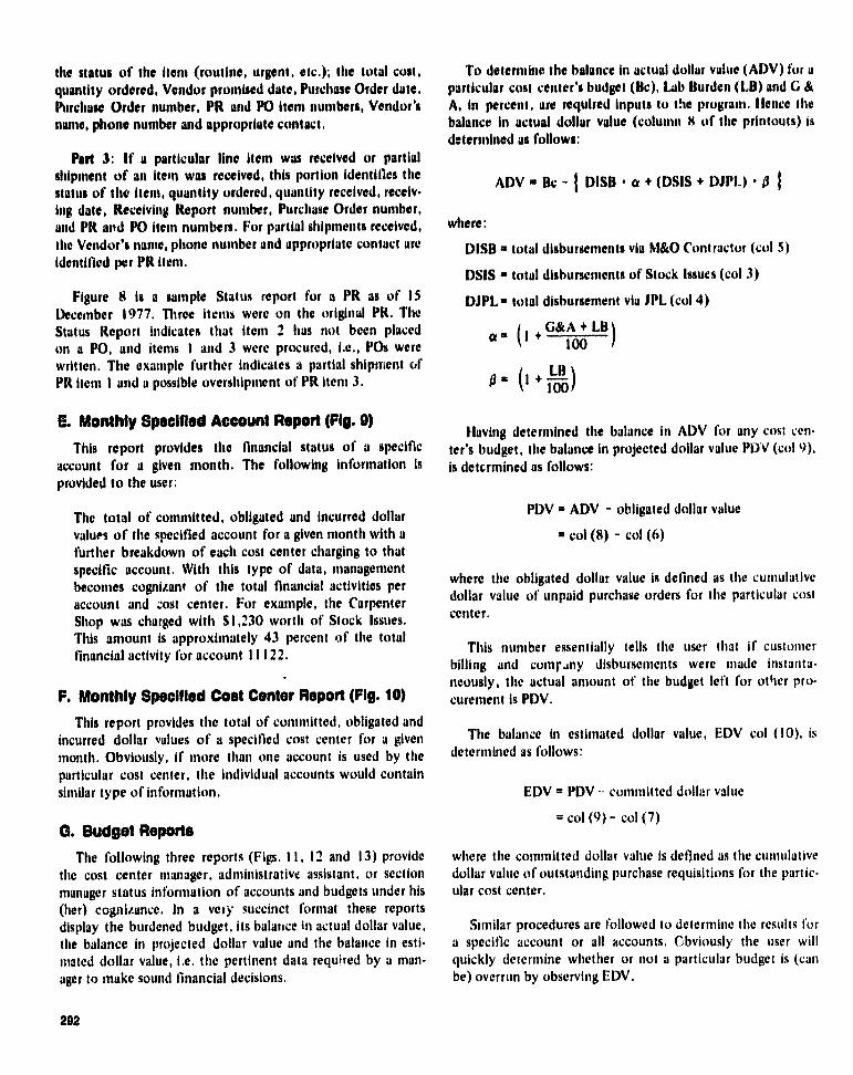
the status of the item (routine, urgent, etc.); the total cost,quantity ordered, Vendor promised date, Purchase Order date,Purchase Order number, PR and PO item ► numbers, Vendor'sname, phone number and appropriate contact.
Part 3: If a particular line item was received or partialshipment of an item was received, this portion identifies thestatus of the item, quantity ordered, quantity received, receiv.ing date, Receiving Report number, Purchase Order number,and PR and PO item numbers, For partial shipments received,the Vendor's name, phone number and appropriate contact areidentified per PR item.
Figure 8 is a sample Status report for a PR as of ISDecember 1977. Three items were on the original PR. TheStatus Report indicates that item 2 has not been placedon a PO, and items I and 3 were procured, i.e., POs werewritten. The example further indicates a partial shipment ofPR item 1 and a possible overshipntent of PR item 3.
S. Monthly Specified Account Report (Fig. ®)
This report provides the financial status of a specificaccount for a given month. The following information Isprovided to the user:
The total of committed, obligated and incurred dollarvalues of the specified account for a given month with afurther breakdown of each cost center charging to thatspecific account. With this type of data, managementbecomes cognizant of the total financial activities peraccount and cost center. For example, the CarpenterShop was charged with $ 1,230 worth of Stock Issues.This amount is approximately 43 percent of the totalfinancial activity for account 11122.
F. Monthly Specified Cost Center Report (Fig. 10)This report provides the total of committed, obligated and
incurred dollar values of a specified cost center for a givenmonth. Obviously, if more than one account is used by theparticular cost center, the individual accounts would containsimilar type of information.
G. Budget ReportsThe following three reports (Figs. 11, 12 and 13) provide
the cost center manager, administrative assistant, or sectionmanager status information of accounts and budgets under his(her) cognizance. In a very succinct format these reportsdisplay the burdened budget, its balance in actual dollar value,the balance in projected dollar value and the balance in esti•mated dollar value, i.e. the pertinent data required by a man-ager to snake sound financial decisions.
To determine the balance in actual dollar value (ADV) for aparticular cost center's budget (Be), Ub Burden (LB) and G &A, in percent, are required Inputs to the program. Hence thebalance in actual dollar value (column 8 of the printouts) isdetermined as follows:
ADV n Be - ; DISH • a + (DSIS + DJPI.) • p 1
where:
DISH ^ total disbursements via M&O Contractor (col S)
DSIS - total disbursements of Stock Issues (col 3)
DJPL- total disbursement via JPL (col 4)
P - ( I + ILA)
Having determined the balance in ADV for any cost cen-ter's budget, the balance in projected dollar value PU'V (col 9),is determined as follows:
PDV - ADV - obligated dollar value
- col (8) - col (G)
where the obligated dollar value is defined as the cumulativedollar value of unpaid purchase orders for the particular costcenter.
This number essentially tells the user that if customerbilling and coniriny disbursements were made instanta-neously, the actual amount of the budget left for other pro-curement is PDV.
The balance in estimated dollar value, EDV col (10), isdetermined as follows:
EDV = PDV committed dollar value
= col (9) - col (7)
where the committed dollar value is defined as the cumulativedollar value of outstanding purchase requisitions for the partic-ular cost center.
Similar procedures are followed to determine the results fora specific account or all accounts. Obviously the user willquickly determine whether or not a particular budget is (canbe) overrun by observing EDV.
292

1. The Specified Account Budget Report (Fig. 11). Thisrepf,rt provides the financial condition of a specified-accountin reference to its budget.
At the end of the report, the cost enters are identified forthe benefit of the user.
The following detail information is provided to the user foreach cost center charging to the specific account:
Cos y.renter Identification Code
Burden Budget
Incurred Dollar Value
Stock Issue (SIS) dollar value
JPL Purchase dollar value
Disbursement charges
Obligated Dollar value
Committed Dollar value
BalanceActual Balance of the cost center budget
Projected Balance of the cost center budget
Estimated Balance of the cost center budget
Having printed the above information per cost center, thefollowing summary information is provided to the user for thespecified account.
Total Burden Budget
Total Stock Issue (SIS) dollar value
Total JPL Purchase dollar value
Total Disbursement charges
Total Obligated dollar value
Total Committed dollar value
Total Actual Balance of the account budget
Total Projected Balance of the account budget
Total Estimated Balance of the account budget
For example, one will note that 10 percent (133,576 actual$ value.) of the total budget for account 1 11322 was spent asof the report date. Approximately 4.8 percent of 133,576 wasused for SIS, 1.3 percent for JPL disbursements, and 3.5percent for M&O Contractor disbursements. The carpentershop spent 40 percent of its budget (3 months into fiscal year)while the Repro shop only disbursed four percent of itsbudget.
2.The Specified Cost Center Budget Report (Fig. 12). Thisreport identifies the financial condition of a specified CostCenter in reference to its budget. The following detail informa-tion is provided to the user:
Account Number(s)
Burden Budget per account
Incurred Dollar Value
Total Stock Issue (SIS) dollar value
Total Ift Purchase dollar value
Total Disbursement (DISB) charges
Total Obligated dollar value
Total Committed dollar value
Balance
Total Actual Balance of the account budget
Total Projected Balance of the account budget
Total Estimated Balance of the account budget
3.All Accounts Budget Report (Fig. 13). This report sum-marizes the financial condition of all accounts in reference totheir respective budgets for which GDSCC Procurement/Financial Planning is responsible. This report will be exten-sively used during budget iterations and financial planning atGoldstone.
The following information is provided to the user byaccounts:
Cost Center Identification Code
Burden Budget
Incurred Dollar Value
Stock Issue (SIS) dollar value
JPL Purchase dollar value
Disbursement charges
Obligated dol'ar value
Committed dollar value
Balance
Actual Balance of the cost center budget
Projected Balance of the cost center budget
Estimated Balance of the cost center budget
ORIGINAL PAGE, Ib 293
OF POOR QUALITY

Summarized at the end of each account's printout is thefollowing account information:
Total Burden Budget
Total Stock Issue (SIS) dollar value
Total JPL Purchase dollar value
Total Disbursement charges
Total Obligated dollar value
Total Committed dollar value
Total Actual Balan ..e of the account budget
Total Projected Balance of the account budget
Total Estimated Balance of the account budget
This report is a true reflection of the budgets from thebeginning of the fiscal year to date. To assist the user inappropriate financial planning decisions, a printout of out-standing PRs and POs are available at the user's request, seeFigs. 14 and 15. Similar backup information is available to theuser upon ter►nination of reports 5 and 7. To reiterate, thepurpose of such backup printouts is to assist the Sectionmanager, cost center supervisor or administrative assistant intheir financial management decision making process. Obvi-ously the above reports, Figs. 11, 12 and 13, give the overviewof a particular budget — i.e. overspent, underspent, or bal-anced. The utility of these backup printouts are left to ;ireGPF financial and management users to establish.
(1/2MM) to prepare an average financial/procurement report.This time includes file searching, sorting, data acquisition, dataverification, processing and report preparation. The burdenedhourly rate for M&O Contractor ntanhours is approximately$14.42/hr. Eight reports are required four (4) (lines a year andthe average cost per report is $1154. The annual preparationcost for these eight GPF financial reports, four times per year,is approximately $37k.
Average report preparation time in the current automatedGPF data base system and the computerized Facility Manage-ment System is four to five minutes. 't he maximum cost of areport generated in the Facility Management System accordingto users was $50. Assuming that the average cost per report inthe GPF data base does not ex eed $50 then the estimatedcost of preparing the identical reports four times a year is$1600 (approximately $2k per year). The $35k or equivalentmanhour savings due to computer generated reports can thenbe applied to other necessary tasks.
From a marginal cost analysis point of view, the net annualdollar savings are shown below.
$ 80k Manpower Reduction — Annual cost savings
+35k Est. Annual Report Preparation cost savings($37k-$2k)
$115k Subtotal Annual Savings
-15k Additional Annual Cost for ComputerServices
$100k Est. Net Annual Savings
III. Estimated Preliminary Savings andAnticipated Benefits
The manual procurement and financial data managementsystem as documented in Ref. (I), consisted of '- JPL person-nel and 4 Contractor personnel. Discussions with GDSCC'sAdministrative Assistant reveals that plans for conversion tothe computerized GPF data base system has resulted in anrrnpower reduction of one JPL and one Contractor typeeffective FY 78. Reduction was in Senior type personnel.Estimated annual burdened manpower savings is $80k which isbased on $50k per JPL MY and $30k per M&O ContractorMY.
Operations costs for the GPF unit, however, must increaseby approximately $12k per year to account for computerservices oil Univac 1 108 system plus an additional $3k peryear for Software maintenance and support.
It was determined during FY 77 by GPF Contractor man-agement that it teak approximately two people one week
In noninflated dollars this estimated net savings is equivalentto $1.0 million over a ten-year life time of the system. Actualdevelopment costs of this computerized data base system isapproximately $90k. The software package is operational andhas been demonstrated during the past year. For the GPFSystem to be operational, certain essential data files must begenerated and the PR files updated as required. It is estimatedthat initial cost to create the basic files for a viable GPF database is less than $10k. Hence, indications are that the com-puterized GPF data management system will pay for itself' inless than one year once the decision has been made to proceedwith final implementation.
Notably, there are other benefits at present which cannotbe quantified monetarily. These anticipated benefits are asfollows:
(1) Basically nonexisting computational errors.
(2) An inherently reliable data base.
294

(3) Timely and pertinent procurement and financial infor- viously available in the GPF manual data managementmation for management decir; om system.
(4) Expanded Anancial reporting ^;apabii.ties not pre-(S) Improved control and visibility of budget and accounts
data.
Reference
Maiocco, F. R. and J. H. Roxek, "An Approach to Improve Management Visibility
Within the Procurement and Financial Group at Goldstone," in Tire Deep SpareNetwork Progress Report 42-35, pp. 171 . 179, Jet propulsion Laboratory, Pasadena,California, October 15, 1976.
295

Table 9. Budget record layout
Table I. Purchase Requlaltlon, purchase order and Item Array Field FormatReceiving Repo" record layout name size
Array Field Cost centers COC 4 A/NItem size Format Cost center name CCN 22 Aname Account
sACC 3 N
Accounts
ACC 5 N Budget° FYB 8 N
Cost center COC 4 A/N Budget entry dates 6 ABudget revision dBudget ate° BRD 4 APurchase requisition number PRN 6 N Cost cantor status CCS 1 APurchase requisition date PRD 6 N
Purchase requisition receiving date RED 6 ,yQuantity requested° QRE 7 N °Stored data of record items can be updated.Unit of measurement
sUNM 2 A —
Item number ITE 2 NUnit price
sUPR 10 N
Status° STA 1 A/NRevision REV I NPurchase order number
sPON 6 N
Purchase order date POD 6 NVendor promise date VPD 6 NVendor code VEN 4 A/N Table 4. Vendor record layoutQuantity ordered° QOR 7 NUnit of measurement
sUMO 2 A Array Field
Purchase order item number ITM 2 N Item name sizeFormat
Purchase order unit prices UPO 10 NReceiving report number RRN 6 N Vendor code
sVC 4 A/N
Receiving date RCD 6 N Vendor names
VN 36 AQuantity received QRC 7 N Address° VA 36 A/NUnit of measurement UMR 2 A Zip code° VZ 5 N
--. Vendor sizes
VS I A°Stored date of record items can be updated. Vendor ratings VR 2 A/N
_ Vendor phone number' VP 10 NVendor contact
sVCT 15 A
°Stored data of record items can be updated.
Table 2. Cost center record layout
Item size FormatArmy Table 6. JPL record layoutCost center
sCOC 4 AN
Cost center namesCCN 22 A Array Field
AccountsACC 5 N Item name size Format
Cost center statusaCCS 1 AAccount ACC 5 N
'Stored data of record items can be updated. Cost center COC 4 A/NDollar amount DOL 9 NDate of entry DOE 6 A
ORIGIN" PAGE Ili
296
OF POOR QUALITY
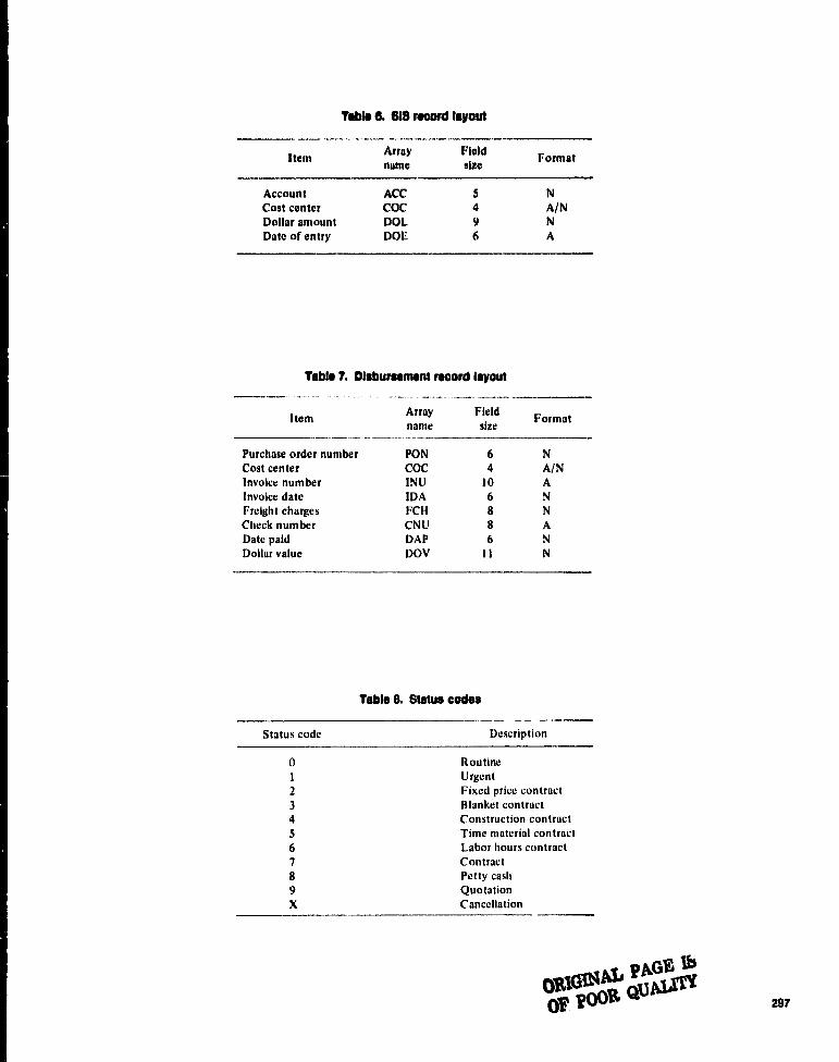
Table & SIB record layout
Item Arrayname
Fieldsize
Format
Account ACC 5 N
Cost center COC 4 A/NDollar amount DOL 9 NDate of entry DOE 6 A
Table 9. Disbursement record layout
ItemArray Field
Formatname size
Purchase order number PON 6 NCost center COC 4 A/NInvoice number INU 10 AInvoice date IDA 6 NFreight charges FCH 8 NCheck number CNU 8 ADate paid DAP 6 NDollar value DOV 11 N
Table 8. Status codes
Status code Description
0 Routine1 Urgent2 Fixed price contract3 Blanket contract4 Construction contract5 Time material contract6 Labor (tours contract7 Contract8 Petty cash
9 (quotationX Cancellation
oRic^^ vGAi TYpF ^4Ug' 297

L
----I
Fig. 1. An overall profile of the automated GDSCC financial/procurement system
298
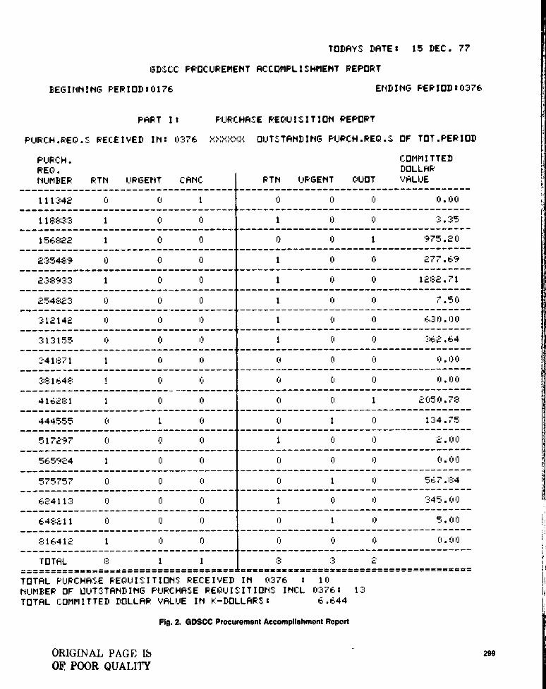
TODAY.S DATE t 15 DEC. 77
GDSCC: PROCUREMENT ACCOMPLISHMENT REPORT
BEGINNING PERIOD=0176 ENDING PERIDDt0376
PART It PURCHASE REQUISITION REPORT
PURCH .RECD . : RECEIVED IN: 0376 r;> :; ; ^,XX OUTSTANDING PURCH . REQ . S OF TOT .PERIOD
PURCH . COMMITTED
REQ. DOLLARNUMBER RTN URGENT CANC: RTN URGENT CAJOT
---------------------------------------VALUE
111342------------------------------
0 0------1
------0 0
---------------------------------------11 11.1111
11 8833------------------------------
1 0 11 1 0 0 3 .35
156)32c 1-------------------------------
0-----'
0 0 0---------------------------------------
---------------------------------------1 975.20
2:35489 (1
------------------------------------0 0 1 0 0
---------------------------------------277.693
23$93 3------------------------------
1 0------rl
-1 0
---------------------------------------0 1 x:. 7 1
25482:3 11
------------------------------0
-----
1.1 1 0 [I 7. 5 11
:312142 0 Il II 1 11 0---------------------------'------------
6.:;11.00
_) 1 ::-., 155 I I------------------------------------
I I 11 1 rl 1)---------------------------------------
j6.` . 6.4
'•41 ;:; 7 1 1-------------------------------------
I1 II I,1 I1 I1 0.00
'%; 154$ 1 II 0 0 0 1) rl . 1) 11
416281 1 0 0 rl rl 1 a 051) . 78
444555 it------------------------------------
1 0 1.1 1---------------------------------
---------------------------------------rl 1: : 4.75
------51 7297 rl
------------------------------11
------
0 1 11
---------------------------------------rl 2.00
565924 1
------------------------------------Cl 0 rl 0 0 11 . ),10
5 5757 it------------------------------------
r1 0 r1 1------------------•---------------------
---------------------------------------rl 5E.7. 84
624113 rl------------------------------------
0 1) 1 rl 0
----------------------------------------=,45.011
64&---'11 0------------------------------
ii------r1
------0 1
---------------------------------------1) 5. 00
;16.412------------------------
1------
II 0 0 rl 0 1) .11 11
TOTAL 1 1 _ _ 2
TOTAL PURCHASE REQUISITIONS RECEIVED IN 0376 10NUMBER OF OUTSTANDING PURCHASE REQUISITIONS I NCL 0376: 13TOTAL COMMITTED DOLLAR VALUE IN K:-DOLLARS: 6.644
Fig. 2. GDSCC Procurement Accomplishment Report
ORIGINAL PAGE IS 299
OF POOR QUALITY

PART III PURCHASE ORDER REPORT
As PURCHASE ORDERS RELEASED (WRITTEN) INt 0376
PURCH. SUBTOTALORDER BLANK SUB. $ PETTY S VALUENUMBER
----RTH---
UPGT----
CONTR-------
VALUE------
CONTR--------
VALUE------
CASH-------
VALUE------
RELEASED-----------------222222 0 1 0 0 0 0 0 0
------30.12
---------338620
---1
----0
----
-------0
-------
------0
------
--------0
-------
-----0
------
--------0
--------0
------
------------37.50
---------339966
---0 0 0 0 1 10276 0 0
------------10275.60
449928 0 0 0-------------
0-------
0------
1 243 243.12---------
666229---
0----
0 1 11060 0 0--------
0------
0------------11060.00
---------882 051
---------
---0
---
----0
----
-------0
-------
------0
------
--------1--------
-----158
-----
--------0--------
------0
------
------------158.16
---------888888 1 0 0 0 0 0 0 0
---29.25
TOTAL 2 1 1 11060 2 10434 1 243
TOTAL NBR.OF PURCHASE ORDERS: RELEASED DURING 0376 7SUBTOTAL DOLLAR VALUE RELEASED IN K—DOLLARS 21.834
Fig. 3. Purchase Order Report
300

Bt OUTSTANDING FURCHASE ORDERS OF TOTAL PERIOD
PURC'H. OBLIGATEDORDER BLANK S SUB. $ PETTY DOLLARNUMBER RTN URGT CONTR VALUE CONTR VALUE CASH VALUE VALUE
128434 0 1 0 0-
0 0-------------
0 0 2.54-
22224:3
---------------------
1 Aw ------------
0 0 0 0-------------
0 0-----------
149.40
261888 1 0 0 0 0 0 0 0------------- 64.6$---------------
_:36i+66----
---0
---
-----A
----
-------------0 0
-------.------
-------------1 10276-------------
0 0------------------
10275.60-----------------
449928 0 1]----
0 0-------------
0 u---
-1 24'3
------------- 243.12---------------------
523-42---
1 0 0 f1----------
0 0 0 A 429.24---------
666229---
0----
0-------------
1 11000-------------
0 0--------------
0 0------------11060.00
---------666441
---------
----1
---
----0
----
-------------0 0-------------
-------------0 0-------------
--------------0 i1
-------------
------------67.20
------------8v2051 0 0 0 1 156 0 0 158.16
TOTAL
of4 1 1 11060 2 104:34 --------------1 24:3
i
------------
NUMBER. OF OUTSTANDING PURCHASE ORDERS INCL 0376 9TOTAL OBLIGATED DOLLAR VALUE IN K—DOLLAR': 22.450
Fig. 4. Outstanding Purchase Order Report
301

TODAY S DATE: 02 NOV. 77
BEGINNING PERIODtOI75
ENDING PERIOD10376
COMMITMENT CATEGORY SUMMARY REPORT
s 0 - 50 0
FLIP[ H . PIJPC H . NU MBER S AMOUNT
ORDER ORDER OF TRAM: IN1 •ILIMBER DATE %vENDOP NAME AC T I0r1 k-,
-----------------------------------------•--------------------------------------7 .474
% 11)9A111 - 250il11(1
PUPC H . P PC H . NUMBER 1. AMOUNT
ORDER ORDER OF TRAM'.- INNUMEER DATE VENDOR NAME ACTION: V-I10LLAR:i•
-------------------------------------------------------------------------------__;'^'=^r_,r, ?2 _76 AACCO ANUFLA ^= TING 1 ►^•c'r'
--------------------------------------------•-----•------------------------------to-#,c2'+ =,277E, A-1 ►--,L:: CTG:.TNG ll.ilr,il
TOTAL OBLIGATED DOLLAR V ALLIE IN k — I► OLLAF': PER REPORTING PERIOD: ^ 1 1 U
— --,lOTE---
THE F q LLOIJ I NG VENDOF' COI+E ! :_ DOE'-, ( D[]') NOT E, ,. I `= T IN 'v'ENDOR—FILE
'',Ehl ,OR CODE PO NUMBER-----------------------------
Allll_1 52:,742H I I I1 = 44'^'a ^'r_^
B 059 G r, I::-,. r:8
Fig. S. Commitment Category Summary Report
PAGE L^ORIGP R, Qt3
OF.
302
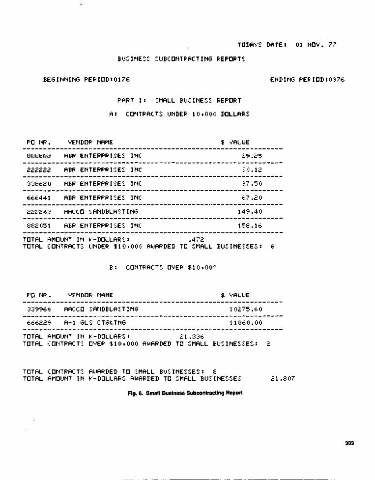
TODAYC DATE 01 NOV. 77
BEGINNING PEPIOD10176 ENDING PERIOD110376
PART Is `-! MALL FUZ.INESS REPORT
R: CONTRACT:-.-,: UNDER 109000 DOLLARS
PC lip . VENDOR NAME--------------------------^-------------------------------------
S VALUE
O88888 HER ENTERPRISES INC 29.25
222222 HER EMTEPPRICES INC--------------------------~---------------------------~--------
_______________________________________________________________30.12
338620 HER EMTERPRI^ES IMCI 37.5V---------~--------------------------------------------~--------
666441 HER EMTERF'R%3EZr INC: 67.20---------------------------------------------------~-----------222243 HH[[O SANDBLASTING 149.40
---------------------------------------------------------------882051 HER EMTEPPRISE1 INC 158.16
---------------------------------------------------------------TOTAL AMOUNT IN V—DOLLRRS: .472TOTAL CONTRR[TC UNDER SI8"0O0 AWARDED TO ^'_--.MHLL DU57-%MESSE2: 6
P: COMTRACY3 OVER S109000
PO MR. VENDOR NAME S VALUE---------------------------------------------------------------
339966 HH[CO CHMDELHST%M6 10275.60_______________________________________________________________
666229 A-1 6L:7. [T6&TNG 11060.00_______________________________________________________________TOTAL AMOUNT IN N—DOLLRRS» 21.3301:TOTAL [OMTR0CTC OVER S10,000 AWARDED TO 'SMALL 0UC1MES3ES: 2
TOTAL COMTRF4[T7_, AWARDED TO CMHLL BUSINESSES: 8TOTAL AMOUNT IN K—DOLLARS 86,18RDED TO :SMALL BUSINESZES 21.807
^^6. Small Business Subcontracting Report

PAPT III LARGE FUSINES:S REPORT
At CONTRACTS UNDER 10+000 DOLLARS
PO NR. VENDOR NAME $ VALUE---------------------------------------------------------------128934 NAT CASH REf S TR 2.54
--------- ------------------------------------------------------TOTAL AMOUNT IN K-DOLLARSt .00:BTOTAL CONTRACTS. UNDER 4109000 AWARDED TO LARGE FUSINESSESt 1
Ft CONTRACTS OVER S10+000
---NOTE---
NO CONTRACTS OVER S10000 AWARDED TO LARGE FUtiINESSES DUPING REPORTING PERIOD
TOTAL C.ONTRAC:TS: AWARDED TO LARGE F;U:: INESS.ES t 1TOTAL AMOUNT IN K-DOLLARS.' AlAARDED TO LARGE BUSINESSES .00:3TOTAL CONTRAC-TS AWARDED IN REPORTING PERIOD: 9TOTAL AMOUNT IN K-DOLLARS. AldARDEI, IN REPORTING, PERIOD 21.810
88.89 PEPC'ENT OF TOTAL AWARDS !dLi4T TO SMALL BUSINES:S.ES'11.11 PERCENT OF TOTAL AIJARDS WENT TO LARGE BUSINESSES99.99 PERCENT OF TOTAL AMOUNT INK—DOLLARS WENT TO ::MALL BU INESSES
.01 FEPCEHT OF TOTAL AMOUNT IN V —DOLLAR:. WENT TO LARGE F-WINE_SES'
---NOTE---
THE FOLLOWING ',VENDOR CODE (S,) DOE'-(DO) NOT EXIST IN VENDOR—FILE
VENDOR CODE PO NUMBER
A 1:10 3 52'3742ACIA3 449928S A59 261888
Fig. 7. Large Business Subcontracting Report
304
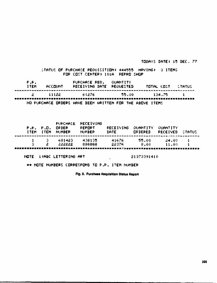
P.R.ITEM
13
sssssssss.
P.O.ITEM
2sessss
TODAYS DATE: 15 DEC. 77
:: TATUS OF PURCHASE REQUISITION: 444555 HAV I NG t 3 ITEMSFOR COST CENTER: 101A REPRO SHOP
P.R. PURCHASE REQ. QUANTITYITEM ACCOUNT RECEIVING DATE REQUESTED TOTAL COST TATUS
--------------------------------------------------------------------------2 11122 e1276 °5.00 134.75 1
ssssssssssssssssssassassssssasssssssssssessssssssssssssssssssssassssssssssNO PURCHASE ORDERS HAVE BEEN WRITTEN FOR THE ABOVE ITEMS
PURCHASEORDERNUMBER
0:,31423222222
sssessssss
RECEIVINGREPORT RECEIVING QUANTITY QUANTITYNUMBER DATE ORDERED PECEIVED STATUS
4:_,81:35 41676 55.00 24.00 1-198888 2237E., 8.00 11 . (19 1
sees:assesseassssss:'ss:esssssszssssssssssssesesssas
NOTE I:ABC LETTERING ART 21373:391410
•• NOTE NUMBERS CORRESPOND TO P.R. ITEM NUMBER
Fig. 8. Purcheee Requisition Status Report
305

TODAY; DATE: 16 DEC. 77
FINANCIAL REPOP'T OF ACCOUNT: 111 22 FOP MONTH OF MAP. 76
CO _;T COMMIT OEL I iG . INCURRED S VALUE TOTAL
CNTP COST CENTER NAME `EVALUE %VALUE ^t'. 13 JPL L I S. SVAL! IE
100A PHOTO LAF 0-------------------------------------------------------------------------------
290 269 0 0 559
1U1A REPRO SHOP 1315----•--------------------------------------------------------------------------
41 0 0 0 116
3i 32A CARPENTER SHOP 1:
-------------------------------------------------------------------------------0 12311.) 0 0 12 3 t^
408A MACHINE SHOP--•., --------------------------------------------------------
'3 0 515:3
--------------------A 0 « r'.
412K COMPLEX SUPPLY 0--------------------------------------------------------------------------------
-------------------------------------------------------------------------------0 :367 1s ij -e- 0--
TOTAL 138 3:,1 2419 0 0 28-.3,3ssssssssssssssssssssssssssssse srsseesasssacs:ssesssssssssssssessscsessescssrsess
Fig. 6. Monthly Specified Account Report
1'OL,A`r'.: DATE: 14 OCT.
FIN144CIA1- PEPOPT FOR CO,:'T CENTEP: 40i-P ! MFCHINE :-HONFOP MONTH OF: MAP. ?'-,
COMMIT. OT:LIG IN0jPPED 1, 'Y1ALLIE TO *14LAC. 0 OI NT S'; ALIJE f Vt;Ll- #E : I _ JF'L III . E- . I'v'AUJ[
aao6eaoe^n:aeo.-ose=-ce^a-ne. nc:o_o_ae.a..eoeeone =-= e....ee.arex=en =eeee=
Fig. 10. Monthly Specified Cost Center Report
ORIGINAL PAGE IbOF POOR QUALITY
306

TODAYS DATEt 16 DEC. 77
BUDGET REPORT FOR ACCOUNTt 11122
COST BUPDErlED INCURRED $ VALUECHTR BUD*ET--------------------------------------
SIB JPL DISB.
1008 8500 330 109 22
101A 6000--------------------------------------
0 89 123
3328 12000 2585 1167 563
408A 19500---------------------------------------
3122 221 4019
412K 102000--------------------------------------
367 132 0
TOTAL 148000--------------------------------------
6404 1718 4727smsssaesmsasssssssssssssssssmssssssssss
BALANCEOBLIG. COMM. ACTUAL PROJEC. ESTIM.$VALUE $VALUE $VALUE $VALUE $VALUE--------
517------
8 7988-----------------
7471------746.E
--------568
------412 5760
-----------------------5192 4780
0 0 7194 7194 7194--------
67--------
------711
------11187
-----------------------11120 10409
0--------
7------
1''1447-----------------------
-----------------101447 101440
------1152 1138 133576 132424 131286
1008 PHOTO LAB1018 REPRO SHOP3328 CARPENTER. SHOP408A MACHINE SHOP412K COMPLEX SUPPLY
Fig. 11. Specified Account Budget Report
TODAYS! DATE: 14 OCT. 77
BiiDGET REPORT FOR i:Q:S:T CENTEF: 408A(MAJ.:HINE 'HOF
'E,HLHN-'EBURDENED INCURRED S W FILUE OBL I 13 . COMM. HC T+JRL PPO.JE':. E.* > T I M .
FKCT . BUDGET : I _AFL D I 'E . 'f VALUE 'f,`,'FIL.UE S s HLI ^ i ^
_ E 'f.: ML JE 'f.:'HI_ JE
1112:: 2'^^OU =^12c c:tl 4G2'3 ^7 i4c^ lll^r lllc:!^ 1:141-
Fig. 12. Specclied Coat Center Budget Report
PAGE lbPRIG ^ QUALITY
®F307

TODAYS DATE: 16 DEC. 77
BUDGED REPORT FOR RCCOUMTt 33119
BALANCECOST BURDENED INCURRED $ VALUE OBLIG. COMM. ACTUAL PROJEC. ESTIM.CNTR BUDGET SIS JPL DISB.
--------------------------------- -----$WALUE $VALUE
------$VALUE-----------------------
$VALUE $VALUE
309D 140U0 0 450 0--------11060 2051 13501 2441 394
TOTAL-------------------------------- ------
14000 0 450 0--------11060
------2051 13501
-----------------2441
------390
mmsammsamssssss sssmasssmmsssssasssssas amsassssamssms sssmmsssmsaassssssassss
:309D COM.CENTER
T7DA`i'S DATE: 16 DEC. 77
BUDGET REPORT FOR ACCOUNT: 45215
=sss==n=nos: __
COST BURDENED INCURRED $ VALUECNTR BUDGET Z, I ZJPL D 11--------------------------------------2:3:3A 1 0000 0 0 0--------------------------------------TOTAL 10400 0 0 0nsoscssnnssnnso=ssscsssnss=ns=nss=nsso
BALANCEPROJEC .$VALUE
9997rf
9997^sasa=sss
E=TIM.$VALUE
'x997
9997osson-==
OBLIG. COMM. ACTUAL$VALUE $VALUE $VALUE
.J rj 10Ci00
2:3:3A FOOD SERVICE
TODAY :=: DATE: 16 DEC. 77
BUDGET REPORT FOR ACCOUNT: 55666
BALANCEACTUAL PROJEC. ES'TIM.$VALUE $VALUE $VALUE-----------------------
2604 2600 2032-----------------------
2644 2600 24:32
C:OS'T BURDENED INCURRED $ VALUECNTR LUDGET I JPL D I SI B .---------------------------------------9766) 2600 0 0 0--------------------------------------TOTAL 2604 4 0 0csonoss0000n-noonoss-s0000=n-nnnsnno-=
97614 CUSTODIAL
Fig. 13. All Acc
OBLIG. COMM.$VALUE $VALUE--------------
0 50- 8--------------
0 568
aunt Budget Report
308

OUTSTANDING PURCHASE REQUISITIONf'AS OF 16 DEC.. 77
COST TOTALCENTER ACCOUNT PR.NUMFER PR.DATE
----------------------------------------------------------STATUS $VALUE
100A 11122 25462:' 12276 O 7.50
10OP 22:341----------------------------------------------------------
a389:: _ :318-76 0 1282.71
101A 11122----------------------------------------------------------
2:3548-9 12376 0 277.69
101A 11122----------------------------------------------------------
444555----------------------------------------------------------
1-18-76 1 134.75
1Q1:'= 11122 312142 11176 0 62;0.00
309I1 _-3119-----------------------------------------------------------
416221----------------------------------------------------------
:2376 9 2050.78-
4ORA 11122 118-11:''?:3 :-31276 0 _ . 5
4088 11122----------------------------------------------------------
31'.155 12376 ii x',2.64
4O8-A 11122----------------------------------------------------------
62411:_ 22376 0 :45.00
4 09D 66622-----------------------------------------------------------
----------------------------------------------------------156122 =2376 9 1;1 115.2 (1
412K: 1 1122 517297 11276 0 2 .01)
412K: 11122----------------------------------------------------------
648-211 11676 1 5.1.10
976b1 55666----------------------------------------------------------
575757 22=76 1 567.:4===ccco=-=c==c=ccocc=a=.=coc=cc===as=ccoc= c.-=c== ==a=c==cc
Fig. 14. Outstanding PR Report
ORIGINAL PAGE ISOF POOR pU AI TY
309

OUT'- THMDQMG PUR[HHZE OPDEVEH^ OF 16 DE[. 77
[O:-- T TOTAL[ENTEP H{[OUMT PO.MUMEEP PO.DATE THTU.- %VHLUE
IVVH 11122----------------------------------------------------------
222243 21476 V 149.4V
1(ICIA 11122----------------------------------------------------------
26 4.69
1V0H 11122---------------------------------------------'------------
449928 32376 8 243.12
1018 11122----------------------------------------------------------
522742 2t976 0 429.24
1V1H 11122__________________________________________________________
----------------------------------------------------------681423 41676 1 74.58
233H 45219 21376 1 2.54
309D 33119----------------------------------------------------------
----------------------------------------------------------666229 32776 3 1I0t.0.(f0
4 08 11122 666441 2t276 0 67.20
409D 66622__________________________________________________________
339966 32376 5 10275.60
41'19 D 66622----------------------------------------------------------
==========================================================051 32376 5 158.16
IF YOU WH-H ADDITIONAL INFORMATION ABOUTH ^PE[lFl[ PUP[HNCE FEQU%CITlOM--PLEH:--7 E LOAD--
377#6PF.PP—^THT—PP6M
Fig. 15. Outstanding PO Report