THE DISPLAY OF INFORMATION AND HOUSEHOLD INVESTMENT

BEHAVIOR

MAYA O. SHATON*

FEDERAL RESERVE BOARD OF GOVERNORS

JULY 29, 2015

ABSTRACT

I show that household investment decisions depend on the manner in which information is

displayed by exploiting a regulatory change which prohibited the display of past returns for

any period shorter than twelve months. In this setting, the information displayed was altered

but the information households could access remained the same. Using a differences-in-

differences design, I find that the shock to information display caused a reduction in the sen-

sitivity of fund flows to short-term returns, a decline in overall trade volume, and increased

asset allocation toward riskier funds. These results are consistent with models of limited at-

tention and myopic loss aversion. To further explore the concept of salience, I propose a dis-

tinction between relative and absolute salience and find evidence consistent with the latter.

Overall, my findings indicate that small changes in the manner in which past performance in-

formation is displayed can have large effects on household investment behavior and potential-

ly influence households’ accumulated wealth at retirement.

* Federal Reserve Board, 20th and C Street, Washington DC 20551. Tel: 202-815-6609. Email: maya.o.shaton@frb.gov.

I am grateful to Nicholas Barberis, Shlomo Benartzi, Cary Frydman, Stefano Giglio, Samuel Hartzmark, Tarek Has-

san, Roie Hauser, Emir Kamenica, Eugene Kandel, Juhani Linnainmaa, Yevgeny Mugerman, Adair Morse, Lubos

Pastor, Jacopo Ponticelli, Amit Seru, Luxi Shen, Kelly Shue, Richard Thaler, Pietro Veronesi, Robert Vishny, Avi

Wohl, Wei Wu and participants at the Whitebox Advisors Graduate Student Conference at Yale, Annual USC Mar-

shall Ph.D. Conference in Finance, LBS 14th Trans-Atlantic Doctoral Conference, Fama-Miller Corporate Finance

Reading Group and the University of Chicago Booth School of Business Finance Workshop, Tel-Aviv University Fi-

nance Seminar, IDC Finance Seminar, EIEF Seminar, Bocconi University Finance Seminar, for many helpful com-

ments. For sharing their data and help, I thank the Capital Market, Insurance, and Savings Department at the Israeli

Minister of Finance, the Investment Department at Israel Securities Authority and Praedicta. I am grateful to Noa

Keysar from the MOF and Yosef Shachnovsky from Praedicta for their help with the data. The views expressed in

this paper are those of the author and do not necessarily reflect the views of the Federal Reserve Bank Board of Gov-

ernors or the Federal Reserve System. All errors are my own.

1. Introduction

In recent decades, households around the world have started playing a more active role in their

retirement savings decisions. Although plans differ, depending on the country and the legal sys-

tem, the shift in investment responsibility to employees is common across many countries. This

shift has prompted a rising interest in both the Economics and Psychology literature on how

individuals make or should make their investments decisions. As retirement savings decisions are

among the key financial decisions individuals make during their lifetimes and may have macro

effects, understanding them is important from a public policy perspective as well.

Traditionally, economic models assume that once information is presented to investors,

they make their decisions based on that information regardless of the exact form it takes.1 None-

theless, a growing literature examining individual choice has found evidence that the manner in

which information is displayed affects individual decision-making.2 For the most part these tests

were conducted in the laboratory or as part of field experiments. Although these controlled set-

tings possess distinct advantages, whether information display will have large effects on real-

world investment behavior remains unclear. At the same time, any tests conducted outside of

controlled settings are typically confounded with a variety of real-world factors making it hard

to disentangle the impact of information display. For example the attainable information set

often varies with information display.

In this paper, I explore how changes to information display affect household trading be-

havior and asset allocation for retirement savings. I exploit a natural experiment in the Israeli

retirement-savings market and show that the manner in which information is displayed has a

strong impact on how the population of investors allocates their retirement savings. In particu-

1 Throughout the paper I distinguish between available and attainable information. I denote as available information the raw information agents observe (the information that “falls from the sky”). Attainable/Accessible information refers to the whole information set to which investors have access. 2 Among others, see Benartzi and Thaler (1999); Thaler, Tversky, Kahneman and Schwartz (1997), Barberis and Huang (2001), Hirshleifer and Teoh (2003), Barber and Odean (2008), Bordalo, Gennaioli and Shleifer (2012), and Beshears, Choi, Laibson, and Madrian (2014). Also see Barberis (2012) for a summary of past studies.

1

lar, starting in 2010, the regulator of Israel’s long-term savings-market prohibited the display of

retirement funds’ returns for any period shorter than twelve months. Previously, 1-month re-

turns were prominently displayed on a monthly basis as a measure of funds’ performance. Fol-

lowing the regulation, the 12-month return is presented to households every month. Households

could also access returns for any horizon longer than twelve months. Although the display of

returns changed, the information set accessible to households did not. Households could still eas-

ily extract the 1-month return from reported information.3 Hence this new regulation represents

a shock to the salience of information rather than a change to the information set accessible to

investors. What makes this a very useful event to study is twofold. First, it is a real-world in-

vestment setting where the manner in which information is displayed changed while the accessi-

ble information set remained constant. Second, I use Israeli mutual funds, which were not sub-

ject to the regulatory change, as my control group.4 More specifically, to control for concurrent

time trends that may have affected trading behavior, I use a differences-in-differences research

design in which retirement and mutual funds are the treated and non-treated groups respective-

ly. Although not identical, I show that the two groups of funds have parallel trends, and thus

mutual funds can serve as the control group in my research design.

My data set combines public data displayed to investors and confidential data collected

by the long-term savings-market regulator. Additionally, I collect performance data for retire-

ment and mutual funds from their monthly reports. This unique dataset permits me to exam-

ine whether and how changes to information display affect households’ investment decisions.

Although the accessible information set remains the same following the new regulation, I find

that households consistently modify their investment behavior. In particular, my results indicate

3 𝑟𝑟𝑡𝑡−1 = 𝑟𝑟𝑡𝑡−13,𝑡𝑡−1+1𝑟𝑟𝑡𝑡−13,𝑡𝑡−2+1 − 1, where rt-1 denotes the lagged one-month return. 𝑟𝑟𝑡𝑡−13,𝑡𝑡−1 denotes the 13-month return from

period t-13 to period t-1, and 𝑟𝑟𝑡𝑡−13,𝑡𝑡−2 denotes the 12-month return from period t-13 to t-2. Both the 12-month and the 13-month returns are still available to households following the regulation. 4 Israeli mutual funds are under the purview of a different regulator, and thus were not subject to the regulation.

2

household behavior is consistent with investors exhibiting limited attention and myopic loss

aversion.

First, I test whether fund flows become less sensitive to past 1-month returns following

the policy change. This test is motivated by Kahneman (1973), who shows that individuals have

limits on the amount of information they can attend to and process. Consequently households

will not use all available information when making investment decisions. Instead households pay

attention to salient or “attention grabbing” information. That is, individuals’ actions are a func-

tion of their attention which in its turn is a function of information’s salience (Plous, 1993). The

regulatory change constitutes a shock to the salience of retirement funds’ past performance in-

formation. By prohibiting the display of 1-month return the regulator rendered these less salient

to households. I show that retirement fund flows were sensitive to past 1-month returns prior to

the regulation. This finding suggests past 1-month returns prior to the salience shock influenced

households’ investment decisions. However, fund flow sensitivity to past 1-month returns signifi-

cantly decreases following the new regulation. In fact, my estimation suggests this sensitivity is

approximately zero after the shock to 1-month returns’ salience.

To better understand how the salience shock influenced households’ attention allocation,

and consequently their behavior, I proceed to examine retirement funds’ trade volumes. Trading

volume represents an observable measure of investors’ attention allocation (Barber and Odean,

2008). Lim and Teoh (2010) explain investors are more likely to trade when they are paying at-

tention to their investments. Accordingly, they consider higher trade volume as resulting from

investors’ attention allocation. My dataset includes all inflows and outflows for the treated and

control funds; thus, I can observe the level of trading for every period. Using the standard dif-

ferences-in-differences specification, I find that trading volume decreased by 30% compared to

the control group following the regulatory change.

The change in performance display is also related to households’ perception of losses. Typi-

cally, losses are more prominent when returns are observed at shorter horizons, e.g., 1-month

3

horizon versus 12-month horizon. Given that empirically 12-month returns tend to be smoother

than 1-month returns if the regulatory change influenced how salient losses are to households, it

may potentially have affected households’ perception of retirement funds’ risk profile. Conse-

quently, we would expect that households invest in riskier funds, conditional on returns, follow-

ing the regulation. I find that net flows into riskier retirement funds increased significantly fol-

lowing the regulation compared to the control group. I show that this net effect primarily results

from a significant increase in flows into riskier retirement funds rather than a decrease in flows

out of these funds. My results are economically significant as well. I find that a one-standard-

deviation shock in a fund’s risk profile, measured by volatility, increases monthly inflows into

such funds by approximately 20%, and decreases the flows out of such funds by approximately

10%. I find similar economic magnitudes using equity exposure as my risk measure; however, in

this case, the estimate for the outflows is not statistically significant.

Finally, I test how the change in information display affected the way fund flows react to 12-

month returns. Theoretically, it is not obvious whether households will react more or less to 12-

month returns after the policy change. This is because evidence from the psychology and neuro-

science literature suggests salience can be decomposed into relative and absolute.5 Absolute sali-

ence refers to salience that arises from some inherent features of the object examined compared

to the rest of the environment. For example, Osberger and Maeder (2001) suggest that some

colors, such as red, draw our attention more than others. In the context of this paper, 12-month

returns are smoother and less flashy than 1-month returns, and are thus less salient in absolute

terms than the 1-month returns. The absolute salience hypothesis predicts households may pay

less attention to their investments in general following the policy change, so the sensitivity of

fund flow to past 12-month returns would decrease.

5 See Mangun (2012) for examples in which such a distinction was made in neuroscience. Jennings and Zeigler (1970) use a similar distinction in a political science study. Manzini and Mariotti (2014) use a similar distinction when mod-eling attention games. According to them: “an attention game with absolute salience is one in which an alternative can decide its own probability of being noticed independently of the salience choices by the other alternatives... When salience is not absolute it is relative”.

4

Relative salience refers to the aspect of salience that depends on how salient the alternatives

examined are. For instance, following the regulatory change, 12-month return is the new default

performance measure, and is thus more salient relative to 1-month return. The relative salience

hypothesis predicts that household may pay more attention to the 12-month return, so the sen-

sitivity of fund flow to past 12-month returns would increase following the policy change. To

test these alternative predictions, I modify the first specification to include the 12-month re-

turns. I find that retirement funds’ flow sensitivity to past 12-month returns significantly de-

creased following the regulatory change compared to the control group. This empirical evidence

is consistent with the notion of absolute salience and suggests households allocate less attention

to their retirement funds’ past performance following the regulatory change.

This paper builds on the literature exploring households’ financial decisions (Campbell,

2006). In particular, it adds to a body of empirical work indicating the importance of infor-

mation display, limited attention and salience on household-behavior. Hirshleifer and Teoh

(2003) show investors attend more to salient items in financial statements. Barber and Odean

(2008) demonstrate that individual investors are more likely to buy rather than sell attention-

grabbing stocks. Bordalo, Gennaioli and Shleifer (2012) present a model of how information sali-

ence affects individual choices under risk. Phillips, Pukthuanthong, and Rau (2014) find that

investors react in a similar way to stale and new information incorporated in mutual funds’

holding period returns. My paper shows that limited attention and salience could have a strong

effect in the context of retirement-savings investment. In particular, I present empirical evidence

that a regulated change in the display of retirement funds’ past performance can significantly

affect households’ trade volume and risk-portfolio allocation. To illustrate the possible magni-

tude of such an impact, I compute a series of simple back-of-the-envelope calculations. I find

that the estimated change to retirement-savings allocation is associated with an increase of 10%

to 20% in total accumulated wealth at retirement for the average 30-year-old household.

5

My paper also relates to the literature discussing how the manner in which information

is displayed influences investors’ perception of losses and consequently their allocation into risky

assets. Past studies have examined how mental accounting and loss aversion affect investor-

behavior (e.g., Thaler et al., 1997; Barberis and Huang, 2001). Benartzi and Thaler (1995) de-

note this combination as myopic loss aversion. A person who declines multiple plays of a simple

mixed gamble to win x and lose y, but accepts it when shown the distribution of outcomes over

the entire set of multiple draws, displays myopic loss aversion. Benartzi and Thaler (1999) pro-

vide experimental evidence suggesting subjects exhibit myopic loss aversion in their retirement

savings.6 Beshears, Choi, Laibson, and Madrian (2014) use a field-experiment to test these earli-

er laboratory experimental results but do not find evidence for myopic loss aversion in their set-

ting. In contrast to previous papers, I estimate the effect of the display of longer-horizon re-

turns using a natural experiment. In line with earlier laboratory experiments, I find that house-

holds increase their allocation into riskier funds when shown longer-horizon returns. To the best

of my knowledge, this paper is the first to provide empirical support for myopic loss aversion

using real-world investment data.

In this paper, I do not claim households act sub-optimally prior to or following the regu-

lation. However, past studies suggest cognitive biases drive investors to engage in wealth-

destroying (e.g., Odean, 1999; Barber, Odean and Zheng, 2000; Frazzini and Lamont, 2008). If

one accepts that behavioral biases have such adverse effects, understanding how information

display can potentially remedy such biases is important from a regulatory perspective. Moreo-

ver, regulating the display of information is relatively benign compared to alternative regulatory

interventions. Specifically, it is less costly compared to other regulatory interventions, such as

financial education (Bertrand and Morse, 2011) and does not generally impose significant costs

6 These studies examined the impact of information aggregation along various dimensions (frequency of information or portfolio level versus asset level information) and found that subjects are more willing to invest in risky assets with positive returns if only the aggregate returns are reported to them. Anagol and Gamble (2013) provide a summary of these various experiments.

6

on agents who do not suffer from any biases in the first place (Camerer et al., 2003; Jolls and

Sunstein, 2006). Third, failure to recognize the effect of the display of information on investors

might lead to granting unwarranted power to the party disclosing information. My results sug-

gest that unsophisticated investors could possibly be manipulated by the mere display of infor-

mation. Discussions surrounding transparency and disclosure requirements are generally cen-

tered on the extent of information given to investors. The results of this paper suggest that the

manner in which information is displayed to investors should be part of such discussions as well.

The rest of the paper is organized as follows: Section 2 describes the institutional back-

ground for the change in regulation and the data. Section 3 describes the empirical methodolo-

gy. In Section 4, I present my results. Section 5 presents a series of robustness tests and Section

6 concludes.

2. Background and Data

2.1 The Israeli Financial Market

In this paper I examine two types of Israeli funds: retirement funds and mutual funds. Specifi-

cally, retirement funds used in this paper are Israeli provident funds (I will refer to these as re-

tirement funds throughout the paper). These retirement funds are a hybrid vehicle combining

features of mutual and pension funds and are used for retirement-savings investment. I limit my

sample to Allowance and Compensation funds. These funds are similar to 401K funds in the

United States; that is, they provide a vehicle for tax efficient retirement savings. However, un-

like 401k plans in the United States, in Israel all investors, employed or self-employed, can in-

vest in any retirement fund and are not restricted to a set offered by their employer. Israeli mu-

tual funds are open-ended mutual funds and are very similar investment vehicle to mutual funds

7

in the United States. It is important to note that in Israel retirement and mutual are two sepa-

rate entities.7

A notable difference between retirement and mutual funds is their respective tax treat-

ment. Retirement funds present several tax benefits that mutual funds do not. The tax treat-

ment of retirement funds is complex, and the specifics depend on the particular circumstances of

each household. Broadly, income invested in retirement funds could entitle households to certain

tax deductions and tax credits. 8 Additionally, households could be exempt from capital gains

tax at redemption if savings are withdrawn in accordance with the regulations.9 Investments in

retirement funds are not liquid and are generally subjected to a 35% tax penalty if withdrawn

early. By contrast, investments in mutual funds are liquid and can be redeemed at any time.

However, such investments are subject to capital gains tax. 10 Mutual funds do offer some tax

advantages. Namely, capital gains tax is due only when the investment in the fund is redeemed

and capital gains can be offset against any capital losses. Although the tax advantages are

greater for retirement funds than mutual funds, these advantages are only applicable up to a

certain level of investment. Above such a level, the benefits significantly decrease. In Section 3, I

elaborate more on the possible repercussions of the different tax treatment for my research de-

sign.

For historical reasons, retirement funds and mutual funds are supervised by different

regulators.11 This distinction in regulatory oversight is key for the empirical strategy I propose

in this paper. Retirement funds are regulated by the Israeli Minister of Finance (MOF). Specifi-

7 In the United States, a mutual fund could have both 401K shares and non-401K shares in the same fund. 8 The level of tax benefits depends, among other things, on: the time the investment was made, income level, em-ployment status, percentage of income saved every month, mean household income and other resources. An important determinant of tax benefits is the income level: the higher the income, the lower are the tax advantages relative to it. 9 The specific form of withdrawal at retirement depends on the time the investment was made and additional sources of income at retirement. Broadly, investment can be withdrawn either as a pension allowance or as a lump sum. Ad-ditionally, in the past, investments could be withdrawn without penalty after a period of 15 years. 10 During the sample period, the capital gains tax was 20% for individuals. Also, certain mutual funds pay taxes at the fund level, and thus investors are exempt from capital gains tax at redemption. However, the number of these funds is small in the sample, and most mutual funds’ tax treatment is as described in this section. 11 Ben Basset (2007) provides background and detailed analysis of the different regulators in the Israeli market.

8

cally, these funds are under the purview of the Capital Markets, Insurance and Savings Division

(CMISD) at the MOF. Retirement funds report monthly their performance to the regulator.

Households can access these data on the MOF’s website – Gemel-Net. 12 Via that website,

households can access performance information for all retirement funds, whether they invested

in them or not. Mutual funds are regulated by the Israeli Securities Authority (ISA). The ISA

oversees the securities sector in Israel, and its range of operations is similar to the SEC in the

United States. The Tel-Aviv Stock Exchange (TASE) is responsible for clearing transactions in

mutual funds. Data on performance and features of mutual funds can be found on the TASE’s

website. Similar to retirement funds, mutual funds are also required to submit monthly reports

to the regulator. These reports are available via the TASE and the ISA websites.

2.2 The Regulation

As described above, households can observe retirement funds’ performance on the MOF’s web-

site, Gemel-Net. Until the end of 2009, the default performance measure displayed on this web-

site was the past 1-month return. In March 2009, the MOF proposed a new regulation prohibit-

ing the display of retirement funds’ returns for any period shorter than twelve months. The in-

tent of this regulation was to allow investors to examine fund’s investment policy over a longer

horizon. The regulator further explained, “These changes are in line with the MOF’s view that

performance of long-term savings vehicles should be measured over a long horizon. Thus it is

important to provide returns’ data for periods greater than 12 months.”

The regulatory change came into effect in January 2010. However, the display of returns

on the Gemel-Net website had already changed in the last quarter of 2009.13 From this point in

time forward, 1-month returns were no longer displayed and 12-month returns became the de-

12 The MOF launched the Gemel-Net website in 2004 and described it as a tool “to allow investors to make informed choices regarding their retirement savings.” The website serves as a reliable source of information regarding retire-ment funds. 13 In this paper, I will use the actual month of the change in display of returns on the Gemel-Net website as the date of the regulation. My results are robust to alternatively defining the date as the date the regulation came into effect.

9

fault performance measure. Figure 1 displays screenshots of the Gemel-Net website prior to

(Panel A) and following the regulation (Panel B).13F

14 The red rectangles emphasize the change in

the manner in which information is displayed to households. We can see in Panel A that prior

to the regulatory change, the default reporting period was one month. Still, households could

deviate from the default and request to see past returns for any longer horizon. Panel B shows

that following the regulation, the default performance horizon changed to twelve months.

Households could still deviate from the default; however, following the regulation they are re-

stricted to a minimum 12-month horizon. Figure 1 shows that the data available to households

following the regulatory change are sufficient to extract the 1-month return. For instance, an

investor can download from the website the 13-month return from period t-13 to period t-1 and

the 12-month return from period t-13 to period t-2. The 1-month return would then equal

𝑟𝑟𝑡𝑡−1 = 𝑟𝑟𝑡𝑡−13,𝑡𝑡−1 +1𝑟𝑟𝑡𝑡−13,𝑡𝑡−2+1 − 1, where 𝑟𝑟𝑡𝑡−1 denotes the lagged one-month return, rt−13,t−1 denotes the 13-

month return from period t-13 to period t-1, and rt−13,t−2 denotes the 12-month return from pe-

riod t-13 to t-2. Both the 12-month and the 13-month returns remain easily accessible to house-

holds following the regulation.

The new regulation pertained to returns displayed on the Gemel-Net website, retirement

funds’ websites, and any marketing materials. In this paper, I mainly refer to the Gemel-Net

website as the source of households’ information. The latter does not weaken my empirical re-

sults, as it reflects how information is displayed following the regulation on other venues as well.

For example, if households observed funds’ performance information on retirement funds’ web-

sites, following the regulation they would no longer be able to see past 1-month returns. In fact,

the regulation was highly enforced across different venues.15 The only exclusion to this regula-

tion is if any unrelated third party displays the information. However, from searches I conduct-

14 I replicated the screenshots and translated it to English as the website is in Hebrew. To emphasize how the new regulation modified the website I focus in this replication on the parts of the website which have changed. 15 I checked different retirement funds’ websites and found next to the display of performance information the follow-ing comment: (translated from Hebrew) “As per regulation we are prohibited from displaying any returns for a period shorter than 12 months.”

10

ed and discussions with government officials, in practice, retirement funds’ 1-month returns were

not widely displayed on public outlets following the regulation.16 Hence, the display of returns

on the Gemel-Net website generally echoes the display on other venues as well.

2.3 Data and Key Variables

The dataset used in this paper is composed of data on retirement funds and data on mutual

funds. Both the ISA and the MOF impose strict reporting requirements on funds. Therefore, the

regulatory change is accompanied by detailed and reliable data of movement of flows, returns,

assets under management, and risk measures. For retirement funds, my data include both pub-

licly available data from the MOF’s website, and confidential data collected by the regulator. As

part of their monthly report to the MOF, all retirement funds disclose flows coming into and

going out of the fund. These data are not publically available; however, I was able to receive

these confidential data from the MOF. To the best of my knowledge, these data have not been

released previously, thus creating an opportunity to explore a novel dataset.17 The mutual funds

dataset includes data provided by Praedicta, an Israeli data-vendor, which I supplemented with

data collected from TASE and ISA’s websites.18

The sample used in this paper is an unbalanced panel data consisting of month-year ob-

servations for the universe of Israeli retirement and mutual funds. Specifically, it includes 347

retirement funds and 1177 mutual funds on average in any given month.19 I exclude from the

dataset mutual funds designed for foreign residents solely, as these funds are less likely to repre-

sent the Israeli household. The sample period begins on January 2008 and ends on December

16 Exceptions would be some very specialized websites I found in searches (and even those were not available initial-ly), but given this paper discusses unsophisticated investors, it is unlikely that the majority would use such websites. 17 The data and results in this paper are presented in accordance to my agreement with the MOF. 18 Specifically, I manually collected the data for the year 2008 for the universe of mutual funds. For the rest of the sample period I relied on the data provided by Praedicta and manually added any missing observations from the ISA and TASE databases. 19 The data are adjusted for any mergers or acquisitions. Therefore, for both retirement and mutual funds the number of funds might vary through the sample period; however, I account for these changes in the data. Overall my dataset includes 424 different retirement funds and 1606 mutual funds. The minimum number of retirement funds in a given month is 317 and the maximum is 388. The minimum number of mutual funds in a given month is 1063 and the max-imum is 1273.

11

2011. The Israeli financial system went through various regulatory reforms in the last decade.

To ensure a similar institutional environment throughout the sample period, I restrict my sam-

ple to 24 months prior to and following the regulation.20 For certain variables, such as monthly

returns, my dataset goes back to 2005. I use these data to compute variables requiring longer

history, e.g., 12-month returns. The data include the following variables: 1-month return, 12-

month return, net fund flow, inflow, outflow, assets under management, volatility of past re-

turns, and equity exposure.

To measure households’ reaction to the regulatory change, I use monthly fund flows

which are actively initiated by households in both the treated and control groups. As noted in

past studies, these flows serve as valuable tools for studying households’ investment decisions.21

Net fund flow is defined as the difference between cashflow into and out of a given fund. One of

the main differences between retirement funds and mutual funds is the composition of their net

fund flow stream. In particular, retirement funds have two additional components: deposits and

withdrawals. Households, investing in retirement funds, deposit a percentage of their income in

the fund each month (𝐷𝐷𝐷𝐷𝐷𝐷𝐷𝐷𝐷𝐷𝐷𝐷𝑡𝑡𝑖𝑖,𝑡𝑡). Households can also withdraw their investment at retirement

age or earlier, but in the latter case they would generally be subjected to a tax penalty

(𝑊𝑊𝐷𝐷𝑡𝑡ℎ𝑑𝑑𝑟𝑟𝑑𝑑𝑑𝑑𝑑𝑑𝑙𝑙𝑖𝑖,𝑡𝑡 ). 22 The last component of retirement fund flow is transfers between funds.

Households can move their retirement savings across retirement funds easily and at a minimal

cost. Savings that are transferred to other retirement funds are not considered withdrawn, and

20 I restricted the sample to begin on January 2008, because this starting point provides a relatively constant legal environment for retirement funds and mutual funds. For example, tax benefits associated with retirement funds were changed at the end of 2007. Also, restrictions on the display of mutual funds past performance were instituted by the ISA in 2007. On January 2012, the capital gains tax increased from 20% to 25%; therefore, to keep the tax treatment relatively constant across the sample period, the last period of the sample is December 2011. 21 The mutual fund literature and the attention literature both use fund flows as measures for investors’ decisions. Chevalier and Ellison (1997) and Sirri and Tufano (1998) use net fund flows in the context of the flow performance relation. Zheng (1999) and Frazzini and Lamont (2008) use net fund flows to test the smart versus dumb money hy-potheses. Barber and Odean, 2008, and Hou, Peng, and Xiong, 2009, use trading volume to proxy for attention. 22 Withdrawals at retirement age can take the form of a one-time withdrawal or pension allowance. The permitted form of withdrawal depends on when the investment was made and the particular circumstances of each household. As noted above, in the past, investments could also be withdrawn without penalty after a period of 15 years; howev-er, this was changed in 2006.

12

thus are not subject to the early-withdrawal tax penalty, and all benefits associated with such

investment are maintained.23 These transfers can be decomposed into money flowing out of a

fund (𝑂𝑂𝑂𝑂𝑂𝑂𝑙𝑙𝐷𝐷𝑑𝑑𝑖𝑖,𝑡𝑡) and money flowing into a fund (𝐼𝐼𝐼𝐼𝑂𝑂𝑙𝑙𝐷𝐷𝑑𝑑𝑖𝑖,𝑡𝑡) . Whereas 𝐷𝐷𝐷𝐷𝐷𝐷𝐷𝐷𝐷𝐷𝐷𝐷𝑡𝑡𝑖𝑖,𝑡𝑡 and

𝑊𝑊𝐷𝐷𝑡𝑡ℎ𝑑𝑑𝑟𝑟𝑑𝑑𝑑𝑑𝑑𝑑𝑙𝑙𝑖𝑖,𝑡𝑡 typically stem from a prescribed rule,24 𝑂𝑂𝑂𝑂𝑡𝑡𝑂𝑂𝑙𝑙𝐷𝐷𝑑𝑑𝑖𝑖,𝑡𝑡 and 𝐼𝐼𝐼𝐼𝑂𝑂𝑙𝑙𝐷𝐷𝑑𝑑𝑖𝑖,𝑡𝑡 require house-

holds to actively change their investment allocation. The monthly deposits and withdrawals

equal zero for mutual funds, but otherwise net fund flow is defined similarly. Specifically, it is

the difference between investors-initiated flows into and out of a given fund.25

The different fund flow composition across the two types of funds could raise concern

over whether mutual funds can serve as the control group in my setting. Additionally, I use net

fund flow as a measure of households’ investment decisions. Thus, another concern that arises is

whether this measure should include deposits and withdrawals, as these typically are not active-

ly initiated by investors. To deal with these possible concerns, I propose removing

𝑊𝑊𝐷𝐷𝑡𝑡ℎ𝑑𝑑𝑟𝑟𝑑𝑑𝑑𝑑𝑑𝑑𝑙𝑙𝑖𝑖,𝑡𝑡 and 𝐷𝐷𝐷𝐷𝐷𝐷𝐷𝐷𝐷𝐷𝐷𝐷𝑡𝑡𝑖𝑖,𝑡𝑡 from retirement fund flow measure. Hence, I define net fund flow

as the difference between cashflow actively moved into and out of a given fund in period t:

𝐹𝐹𝐹𝐹𝑖𝑖,𝑡𝑡 = 𝐼𝐼𝐼𝐼𝑂𝑂𝑙𝑙𝐷𝐷𝑑𝑑𝑖𝑖,𝑡𝑡 − 𝑂𝑂𝑂𝑂𝑡𝑡𝑂𝑂𝑙𝑙𝐷𝐷𝑑𝑑𝑖𝑖,𝑡𝑡. In addition, to show that my results are not driven from my

choice of definition, I repeat my estimations using the actual net fund flow. 𝐹𝐹𝐹𝐹𝑉𝑉𝑖𝑖,𝑡𝑡 denotes this

second measure: 𝐹𝐹𝐹𝐹𝑉𝑉𝑖𝑖,𝑡𝑡 = �𝐼𝐼𝐼𝐼𝑂𝑂𝑙𝑙𝐷𝐷𝑑𝑑𝑖𝑖,𝑡𝑡 + 𝐷𝐷𝐷𝐷𝐷𝐷𝐷𝐷𝐷𝐷𝐷𝐷𝑡𝑡𝑖𝑖.𝑡𝑡� − �𝑂𝑂𝑂𝑂𝑡𝑡𝑂𝑂𝑙𝑙𝐷𝐷𝑑𝑑𝑖𝑖,𝑡𝑡 + 𝑊𝑊𝐷𝐷𝑡𝑡ℎ𝑑𝑑𝑟𝑟𝑑𝑑𝑑𝑑𝑑𝑑𝑙𝑙𝑖𝑖.𝑡𝑡� . Both 𝐹𝐹𝐹𝐹𝑖𝑖,𝑡𝑡

and 𝐹𝐹𝐹𝐹𝑉𝑉𝑖𝑖,𝑡𝑡 are measured in millions of New Israeli Shekel (NIS), the domestic currency. That is,

in my estimations below, the impact of a $100 flow into a fund that has $100 under manage-

23 I adjust this value for any transfers to other savings vehicles in the long-term savings market. Additional long-term savings instruments are pension funds and life insurance contracts. In the past few years, households were permitted to transfer their savings between retirement funds and these additional instruments. However, in my dataset, I find that the majority of transfers are between retirement funds. My data allow me to separate between these vehicles; however, the inclusion of these two additional instruments does not change my results as transfers to these were mi-nor during my sample period. 24 For instance, such a rule could be that 5% of one’s income is invested in its retirement fund every month. Another example is when a household reaches retirement age and starts receiving a pension allowance. A notable situation of withdrawals resulting from households’ actions is the case of early withdrawal. However, given the high penalty asso-ciated with it, it is reasonable to assume that such decisions are not driven by fund specific characteristics that would bias the results, but rather by some household-specific circumstances. 25 In the case of mutual funds, these flows will represent both transfers between funds and new money coming into the market. However, these flows are similar to transfers in retirement funds, because investors actively initiate them.

13

ment will equal the impact of a $100 flow into a fund with $1000 under management.26 There-

fore, I propose additional measures of net fund flow scaled by fund size. To prevent large chang-

es in the denominator from influencing my results, I approximate fund size by the average asset

under management during the sample period. 27 𝐹𝐹𝐹𝐹𝑆𝑆𝑖𝑖,𝑡𝑡 and 𝐹𝐹𝐹𝐹𝑉𝑉 𝑆𝑆(𝑖𝑖,𝑡𝑡) denote these scaled

measures of net fund flow.28 Following Spiegel and Zhang (2013) and Huang, Wei and Yan

(2007), in order to prevent potential impact of outliers resulting from data errors, I winsorize

the top and bottom 2% tails of the net fund flow data.29

𝑂𝑂𝑂𝑂𝑡𝑡𝑂𝑂𝑙𝑙𝐷𝐷𝑑𝑑𝑖𝑖,𝑡𝑡 and 𝐼𝐼𝐼𝐼𝑂𝑂𝑙𝑙𝐷𝐷𝑑𝑑𝑖𝑖,𝑡𝑡 represent flows that households actively initiate. Accordingly, I

define the volume of trading activity as the absolute sum of these two variables: 𝑇𝑇𝑟𝑟𝑑𝑑𝑑𝑑𝐷𝐷𝑖𝑖,𝑡𝑡 =

𝐼𝐼𝐼𝐼𝑂𝑂𝑙𝑙𝐷𝐷𝑑𝑑𝑖𝑖,𝑡𝑡 + 𝑂𝑂𝑂𝑂𝑡𝑡𝑂𝑂𝑙𝑙𝐷𝐷𝑑𝑑𝑖𝑖,𝑡𝑡. Same as for net fund flow, I scale trade volume by fund’s average asset

under management during the sample period. 𝑇𝑇𝑟𝑟𝑑𝑑𝑑𝑑𝐷𝐷𝑆𝑆𝑖𝑖,𝑡𝑡 denotes the scaled trade volume.

In the setting of the natural experiment used in this paper, households observe gross re-

turns. Accordingly, I use gross returns in my estimations. 𝑟𝑟𝑖𝑖,𝑡𝑡−1 denotes the lagged 1-month re-

turn and 𝑟𝑟𝑖𝑖,[𝑡𝑡−12,𝑡𝑡−1] denotes the 12-month return from period t-12 to period t-1. The return is

computed daily as the return on assets under management. Then the daily return is compound-

ed to 1-month return and 12-month return.30 Assets under management are reported by funds as

their value at the end of each month. I use assets under management at the end of the previous

26 At the same time, using fund flow scaled by fund size could lead to other concern. I expand on this in Section 4.1. 27 I obtain qualitatively similar results when I approximate fund size using asset under management at the beginning of the sample period. 28 In the mutual fund literature, net fund flows are typically approximated using the percentage growth in total net asset value in excess of return (see, e.g., Sirri and Tufano, 1998). However, my dataset includes data on fund flows; thus, I do not use this approximation. 29Huang, Wei, and Yan (2007) refer to errors associated with mutual fund mergers and splits in US mutual fund data. However, the same reasoning applies to Israeli mutual fund data as well. Therefore, to avoid any impact of data error on my results I winsorize my dataset. Nonetheless, my results are robust to this winsorization. 30 According to Israeli tax regulations retirement fund monthly return is computed in the following way: 𝑌𝑌𝑚𝑚𝑚𝑚𝑚𝑚𝑡𝑡ℎ = [(𝑌𝑌1 + 1) ∗ (𝑌𝑌2 + 1) ∗ …∗ (𝑌𝑌𝑚𝑚 + 1) − 1], where 𝑌𝑌1 …𝑌𝑌𝑛𝑛 are daily returns, and n is the number of business days in a given month. Daily returns are defined as: 𝑌𝑌𝑑𝑑𝑑𝑑𝑖𝑖𝑑𝑑𝑑𝑑 = �𝐴𝐴𝐴𝐴𝐴𝐴𝐴𝐴𝑡𝑡𝐴𝐴1−𝐻𝐻

𝐴𝐴𝐴𝐴𝐴𝐴𝐴𝐴𝑡𝑡0−𝑀𝑀 − 1�, where Assets0 equals the assets under management as of the end of the previous day; Assets1 equals the assets under management as of the end of the day of the compu-tation; H equals all cash that is deposited in the fund at the end of the day; and M equals the total amount of cash that was withdrawn from the fund throughout the day. 12-month returns are computed in the same way: 𝑌𝑌𝑑𝑑𝑚𝑚𝑚𝑚𝑎𝑎𝑑𝑑𝑑𝑑 =[(𝑌𝑌𝑚𝑚𝑚𝑚𝑚𝑚𝑡𝑡ℎ1 + 1) ∗ (𝑌𝑌𝑚𝑚𝑚𝑚𝑚𝑚𝑡𝑡ℎ2 + 1) ∗ … .∗ (𝑌𝑌𝑚𝑚𝑚𝑚𝑚𝑚𝑡𝑡ℎ12 + 1) − 1], where Ymonth,t equals the monthly return at period t. Mutual funds returns are computed in a similar way.

14

period to control for fund size in period t. 𝐴𝐴𝐴𝐴𝑀𝑀𝑖𝑖,𝑡𝑡−1 denotes the assets under management for a

given fund at the beginning of period t. I require that all observations have non-missing values

for 𝑟𝑟𝑖𝑖,𝑡𝑡−1 and 𝐴𝐴𝐴𝐴𝑀𝑀𝑖𝑖,𝑡𝑡−1. I further restrict my sample to observations with AUM values larger

than zero at the beginning of period t.

Table 1 reports the summary statistics for my sample. We can see that the typical re-

tirement fund size is greater than the typical mutual fund size. Specifically, the average retire-

ment fund has $116.7 million in AUM, whereas the average mutual fund has $30.3 million in

AUM. Additionally, we see that the average retirement fund trade volume is $1.9 million, while

the average mutual fund has a trade volume of $5.163. I address these differences below when

formulating my empirical design. The retirement and mutual fund industries are significant in

the Israeli capital market. 𝑇𝑇𝐷𝐷𝑡𝑡𝑑𝑑𝑙𝑙𝐴𝐴𝐴𝐴𝑀𝑀𝑡𝑡 denotes the aggregate AUM for all funds in my sample in

period t. During the sample period, the aggregate AUM for retirement funds is on average 150

NIS (approximately 40.5 billion USD) and the aggregate AUM for mutual funds is on average

134 billion NIS (approximately 36 billion USD). Together these markets represent approximate-

ly 35% of Israel’s GDP.31

Table 2 reports the different categories of retirement funds (Panel A) and mutual funds

(Panel B). Panel A shows that the majority of retirement funds are general funds. According to

Panel B, most mutual funds are fixed-income funds. 23% of mutual funds and 11% of retirement

funds are classified as equity funds. However, the broad definition of fund categories makes dis-

cerning fund investment policy by looking only at the categories difficult. For instance, a general

retirement fund could invest 30% or 1% in equity. Therefore, to better understand fund risk-

profile both regulators, the MOF and ISA, require funds to monthly report their equity exposure

starting 2008.32 Equity exposure is defined as the fraction of AUM held in equity and in deriva-

31 During the sample period 1 NIS equaled on average 0.27 USD. 32 The ISA, regulator of mutual funds, explained the reasoning for the regulation: “to help investors understand more about the portfolio of funds” (translated from Hebrew).

15

tives whose underlying asset is equity. This ratio is displayed to households on the MOF and

TASE’s websites for retirement and mutual funds, respectively. 𝐸𝐸𝐸𝐸𝑖𝑖,𝑡𝑡 denotes fund i equity ex-

posure in period t. It is important to note that fixed-income funds can be relatively safe, invest-

ing in government bonds, or more risky, investing in corporate bonds. Such risk will not be re-

flected in the equity exposure measure; therefore, to provide a cleaner measure of fund risk-

profile, I also use the volatility of past returns. To mirror the volatility displayed to households,

I compute the volatility using the previous thirty-six months 1-month returns. I denote this var-

iable as 𝑉𝑉𝐷𝐷𝑙𝑙𝑖𝑖,𝑡𝑡. Table 1 shows that 23% of the average retirement fund’s AUM are exposed to

equity, and its volatility measure equals 2.3%. Whereas 29% of the average mutual fund’s AUM

are exposed to equity and its volatility measure equals 2.5%. Therefore, although Table 2 could

suggest that the two groups of funds have very different investment policies, we see that on av-

erage their risk profiles are not as different.

3. Empirical Methodology

This paper exploits the regulatory change, described in the previous section, to identify how the

manner in which information is displayed impacts household investment behavior. Although this

effect could be important, identifying it outside of controlled experimental settings is challeng-

ing. First, it is difficult to find a natural setting where the display of information has changed

while the attainable information set remains constant. When both the attainable information set

and the display are changed simultaneously, disentangling any effect of the display of infor-

mation from the impact of the change in the information set becomes hard. Second, even if one

finds such a natural experiment, identifying the effect of a change to information display could

remain difficult given potential unobservable factors. For example, it is possible that unobserved

contemporaneous shocks to local market conditions affect household-behavior irrespective of any

changes to information display. Thus, claiming causality could prove to be complex.

16

The proposed research design overcomes these two challenges. First, I present a natural

experiment where the manner in which information is displayed has changed while the attaina-

ble information set remained constant. Specifically, the regulatory change prohibited the display

of retirement fund past 1-month returns and rendered the 12-month return the new default per-

formance measure. Still, households could extract the 1-month return from the attainable data.

Hence, the change to information display is not associated with changes to the attainable infor-

mation set. Accordingly, this setting provides a real-world investment environment that over-

comes the first identification challenge presented. Second, I use mutual funds, which were not

subject to the regulation, to control for unobserved omitted variables. In particular, I implement

a differences-in-differences (DD) methodology to isolate the causal effect of the change in infor-

mation display from any other confounding factors. If valid, this empirical design permits me to

overcome the second challenge presented. Although both groups of funds are similar investment

vehicles, as we saw in Table 1, they are not identical. Nevertheless, the proposed experimental

design is valid as long as the parallel trend assumption holds. That is, if both groups of funds

would display similar trends absent the regulatory change.

Using the proposed empirical strategy, I construct three main specifications, each analyz-

ing different possible impacts of the regulatory change. In particular, I implement the DD ap-

proach to estimate the effect of shocks to information display on: 1) fund flow sensitivity to past

performance, 2) trading volume, and 3) portfolio risk allocation. These specifications build upon

mutual funds serving as the control group. Therefore, before elaborating on those in Section 4,

for the remainder of this section, I discuss whether mutual funds are an appropriate control

group in my setting.

The key threat to the empirical design is a possible time-varying group-specific shock

that may coincide with the regulatory change to information display. However, I argue this

threat is limited in the context of this paper. To support my argument, I begin by discussing a

range of variables which could potentially give rise to this threat. In light of the novelty of my

17

dataset such discussion is valuable to clarify all relevant details. In Section 4, I address these

concerns when formulating my empirical tests.

As discussed in Section 2, retirement and mutual funds are subject to different tax

treatment. Namely, investment in a retirement fund is associated with various tax benefits if not

withdrawn early. Accordingly, the investment horizon would likely differ across these two types

of funds. Thus, a possible concern is that the two groups of funds undertake different invest-

ments on average and will be exposed to different market shocks throughout the sample period.

While this concern is compelling in theory, it is not prominent in the setting presented. In fact,

the majority of investment in retirement funds has already matured and is eligible to be with-

drawn without losing the associated tax benefits. Consequently, similar to mutual funds, retire-

ment funds’ AUM need to be relatively liquid.33 This last conjecture is supported in the empiri-

cal data. Figure 3 presents the distribution of AUM across different classes of investment for

the treatment and control group for the first period in my dataset. We can see that mutual

funds do invest a large percentage of their AUM in liquid assets such as cash and cash equiva-

lent. However, Figure 3 also reveals the composition of AUM is not as different as one could ex-

pect. These data suggest that on average, AUM composition does not expose retirement and

mutual funds to different market shocks throughout the sample period. This argument is further

supported by examining the average return of the two groups of funds. Table 1 shows that,

throughout the sample period, the average retirement and mutual funds presented similar 1-

month and 12-month returns. The average 1-month and 12-month returns for retirement funds

were 0.28% and 5.6%, respectively, whereas mutual funds’ average 1-month and 12-month re-

turns were 0.212% and 5.2%, respectively. Figure 2 presents the time series of the average 1-

month and 12-month returns for both types of funds. We can see these return series tend to

move together. The correlation between retirement and mutual funds’ average monthly returns

33 According to numerous reports, approximately 70% of retirement funds’ assets under management are eligible for withdrawal.

18

is 0.9827, and the correlation between their 12-month returns is 0.9893. This evidence provides

further support that retirement and mutual funds are impacted similarly by market conditions

during the sample period. Both the investment allocation of AUM and the achieved returns help

alleviate concerns that the different nature of the two types of funds is undermining the empiri-

cal design proposed.

Another potential concern is that heterogeneity in wealth and sophistication level of in-

vestors across the treated and control groups would expose the two to different time-varying

shocks. In contrast to the case in other countries, in Israel the investor populations in retirement

and mutual funds are relatively similar and tend to overlap.34 They are both retail investors and

they typically belong to the top half of the Israeli income distribution.35 In addition, the regula-

tory change was not accompanied by any institutional innovations that would induce changes to

the composition of investor populations during my sample period. Therefore, it is plausible to

assume that investors’ sophistication level remains constant throughout the sample period.

Thus, any possible difference in sophistication level across the treated and control groups would

likely be addressed by the DD approach.

Finally, graphical inspection of parallel trends indicates smooth pretrends and a clear

break for the treatment group following the regulatory change. Figure 5 plots the average trade

volume scaled by fund size for the treated and control groups. We can see that both groups

show parallel trends prior to the regulatory change. Following the regulatory change, retirement

funds’ trade volume drops while the trade volume of mutual funds continues to grow. Figure 5

demonstrates that the parallel trend assumption holds in the data, thus indicating the proposed

empirical design is valid.

34 This is based on information received from the regulator. Typically, mutual funds’ retail investors also hold retire-ment funds. While the opposite is not necessarily true, it is likely to occur. The latter is resulting from various rea-sons such as the different tax treatment along the income distribution. A contribution factor to this composition is that historically these retirement funds were used largely by wealthier self-employed individuals. 35 According to the Israeli Central Bureau of Statistics, in 2008 the average income for employees who save for re-tirement was three times larger than for employees who do not (approximately $3000 per month versus $1000 per month for employees who do not save. For reference the average income in Israel in 2008 was approximately $2200 per month).

19

4. Results

In this section, using the empirical design discussed above, I estimate how shocks to information

display impact household behavior. Past research has shown that attention is a limited resource.

Hence, households will not use all available information when making their investment deci-

sions.36 Instead, households pay attention to salient or “attention grabbing” information. That

is, households’ investment decisions depend on attention which is in turn a function of salience.

Accordingly, shocks to information salience would impact attention allocation and subsequently

household behavior. The regulatory change constitutes a shock to the salience of past returns

along several dimensions. First, it prohibited the display of past 1-month return which was

prominently displayed prior to it. Thus, the regulation rendered past 1-month returns less sali-

ent to households. Second, the regulatory change resulted in the past 12-month return becoming

the default performance measure. 12-month returns are inherently different from 1-month re-

turns. If this difference affects how salient information is to households, it could potentially im-

pact household behavior. I elaborate on this argument in Sections 4.3 and 4.4.

4.1 Shock to Salience and Fund Flow Sensitivity to Past Performance

I begin by examining how the regulatory shock to the salience of past 1-month returns impacts

households’ investment decisions. To measure how households react to the change in the display

of returns, I use the flow-performance relation from the mutual funds’ literature. Past research

has shown that investors use mutual funds’ past performance when making their investment-

decisions (Sirri and Tufano, 1998; Ippolito, 1992; Chevalier and Ellison, 1997). This return-

chasing behavior has been mainly documented using US mutual fund data, however similar find-

ings were observed across countries (Ferreira, Keswani, Miguel, and Ramos, 2012). Specifically,

in the Israeli context Ben-Rephael, Kandel and Wohl (2011) find evidence of return-chasing be-

36 For survey of this literature see Lim and Teoh (2010) and DellaVigna (2009).

20

havior in Israeli mutual funds, and Steinberg and Porat (2011) show similar behavior in Israeli

retirement funds using data prior to the regulatory change. Therefore, I combine the flow per-

formance relation with the empirical methodology discussed in Section 3 to estimate the effect of

the regulatory change on household return-chasing behavior.

The regulation prohibited the display of past 1-month returns which were prominent

previously. However, as noted earlier, households could still extract the 1-month return from the

accessible information set. That is, the regulation altered how salient past 1-month return is to

households, while not restricting households from this information. According to the decision-

making mechanism described above, a decline in salience of past 1-month returns could reduce

the attention allocated to these returns. The latter would in turn influence households’ invest-

ment decisions. As noted in Section 2, I use flows actively initiated by households as my main

measure of households’ investment decisions. The sensitivity of fund flow to past 1-month return

serves as my proxy for households’ attention. That is if households pay less attention to 1-

month return following the salience shock, fund flow sensitivity to past 1-month return would

decrease (Hypothesis 1). To empirically test this hypothesis, I propose the following DD specifi-

cation:

𝐹𝐹𝑂𝑂𝐼𝐼𝑑𝑑𝐹𝐹𝑙𝑙𝐷𝐷𝑑𝑑𝑖𝑖,𝑡𝑡 = 𝛽𝛽1𝑟𝑟𝑖𝑖,𝑡𝑡−1 + 𝛽𝛽2�𝑟𝑟𝑖𝑖,𝑡𝑡−1 × 𝑃𝑃𝐷𝐷𝐷𝐷𝑡𝑡𝑡𝑡� + 𝛽𝛽3�𝑟𝑟𝑖𝑖,𝑡𝑡−1 × 𝑅𝑅𝐹𝐹𝑖𝑖�

+ 𝛽𝛽4�𝑟𝑟𝑖𝑖,𝑡𝑡−1 × 𝑃𝑃𝐷𝐷𝐷𝐷𝑡𝑡𝑡𝑡 × 𝑅𝑅𝐹𝐹𝑖𝑖� + 𝛽𝛽5(𝑃𝑃𝐷𝐷𝐷𝐷𝑡𝑡𝑡𝑡 × 𝑅𝑅𝐹𝐹𝑖𝑖)

+ 𝐶𝐶𝐷𝐷𝐼𝐼𝑡𝑡𝑟𝑟𝐷𝐷𝑙𝑙𝐷𝐷 + 𝛼𝛼𝑖𝑖 + 𝛿𝛿𝑡𝑡 + 𝜖𝜖𝑖𝑖,𝑡𝑡,

(1)

where 𝐹𝐹𝑂𝑂𝐼𝐼𝑑𝑑𝐹𝐹𝑙𝑙𝐷𝐷𝑑𝑑𝑖𝑖,𝑡𝑡 denotes different measures of net fund flow in period t as described below.

The independent variables are lagged 1-month return 𝑟𝑟𝑖𝑖,𝑡𝑡−1, 𝑃𝑃𝐷𝐷𝐷𝐷𝑡𝑡𝑡𝑡, 𝑅𝑅𝐹𝐹𝑖𝑖, and interaction terms

between these variables. 𝑃𝑃𝐷𝐷𝐷𝐷𝑡𝑡𝑡𝑡 is an indicator variable which equals 1 if the observation is in a

period following the regulatory change, and 0 otherwise. 𝑅𝑅𝐹𝐹𝑖𝑖 is an indicator variable that equals

1 if fund i is a retirement fund, and 0 if it is a mutual fund. (𝑟𝑟𝑡𝑡−1 × 𝑃𝑃𝐷𝐷𝐷𝐷𝑡𝑡𝑡𝑡) is an interaction term

21

between lagged 1-month return and the indicator variable 𝑃𝑃𝐷𝐷𝐷𝐷𝑡𝑡𝑡𝑡. (𝑟𝑟𝑡𝑡−1 × 𝑅𝑅𝐹𝐹𝑖𝑖) is an interaction

term between lagged 1-month return and the indicator variable 𝑅𝑅𝐹𝐹𝑖𝑖. (𝑟𝑟𝑡𝑡−1 × 𝑃𝑃𝐷𝐷𝐷𝐷𝑡𝑡𝑡𝑡 × 𝑅𝑅𝐹𝐹𝑖𝑖) is an

interaction term between lagged 1-month return and the indicator variables 𝑃𝑃𝐷𝐷𝐷𝐷𝑡𝑡𝑡𝑡 and 𝑅𝑅𝐹𝐹𝑖𝑖 .

𝐶𝐶𝐷𝐷𝐼𝐼𝑡𝑡𝑟𝑟𝐷𝐷𝑙𝑙𝐷𝐷 denote in this specification solely a control for fund size. 𝛼𝛼𝑖𝑖 and 𝛿𝛿𝑡𝑡 are fund and

month-year fixed effects, respectively. 𝜀𝜀𝑖𝑖,𝑡𝑡 is the regression residual. The inclusion of control for

size and fund fixed effect help remedy concerns, noted earlier, that differences between the

treated and the control group would influence my results. Further, time fixed effects address

concerns that any periodic shock would undermine my estimated coefficients.

I estimate the regression in Eq.1 using different measures for net fund flow. As defined in

Section 2, 𝐹𝐹𝐹𝐹𝑖𝑖,𝑡𝑡 and 𝐹𝐹𝐹𝐹𝑉𝑉𝑖𝑖,𝑡𝑡 denote the NIS (dollar) value of net fund flow and 𝐹𝐹𝐹𝐹𝑆𝑆𝑖𝑖,𝑡𝑡 and

𝐹𝐹𝐹𝐹𝑉𝑉 𝑆𝑆𝑖𝑖,𝑡𝑡 denote fund flow scaled by fund size. Zheng (1999) uses dollar amount of fund flow ra-

ther than percentage values. He argues that dollar amount represents a better measure when

aggregating fund flow performance across funds from the perspective of investors. Typically, in

the mutual fund literature, net fund flow measures are scaled by fund size as discussed in Sec-

tion 2 (Sirri and Tufano, 1998). Spiegel and Zhang (2013) argue that this commonly used per-

centage flow measure fails to consider the effect of aggregate investor allocation when testing the

flow performance relation. Instead, they propose using growth in fund’s market share as the de-

pendent variable.37 To show that my results are robust, I estimate the specification in Eq.1 us-

ing different fund flow measures presented in the literature. 38 This could be valuable in the con-

text of this paper. As on the one hand, using dollar amount of fund flow could lead to unwar-

ranted impact of small funds, as noted in the example above. While on the other hand, aggrega-

tion concerns could undermine my results.

37 Following their methodology 𝑀𝑀𝑀𝑀𝑀𝑀𝑆𝑆𝑖𝑖,𝑡𝑡 denotes the growth in market share of fund i in period t measured times 10000: 𝑀𝑀𝑀𝑀𝑡𝑡𝑆𝑆𝑖𝑖,𝑡𝑡 = 𝐴𝐴𝐴𝐴𝑀𝑀𝑖𝑖,𝑡𝑡

𝑇𝑇𝑚𝑚𝑡𝑡𝑑𝑑𝑑𝑑𝐴𝐴𝐴𝐴𝑀𝑀𝑡𝑡− 𝐴𝐴𝐴𝐴𝑀𝑀𝑖𝑖,𝑡𝑡−1

𝑇𝑇𝑚𝑚𝑡𝑡𝑑𝑑𝑑𝑑𝐴𝐴𝐴𝐴𝑀𝑀𝑡𝑡−1.

38 When using growth in market share, the sensitivity of growth in market share to past 1-month return will serve as my proxy for households’ attention allocation.

22

Table 3 reports the estimates from the regressions of the form in Eq.1. The main coeffi-

cient of interest in this specification is 𝛽𝛽4. This coefficient identifies the causal impact of the

regulatory change on the proxy for households’ attention. In line with the presented hypothesis I

expect to find 𝛽𝛽4 < 0. Columns 1-5 report the coefficient estimates using the five measures of

net fund flow described above. For all five measures, I find that the estimator 𝛽𝛽4 is negative and

statistically significant. That is, retirement fund flow sensitivity to past 1-month return signifi-

cantly decreases compared to the control group following the salience shock. I find the same ef-

fect when using growth in market share as the dependent variable. The coefficient estimate for

𝛽𝛽4 equals -0.608 when 𝐹𝐹𝐹𝐹𝑖𝑖,𝑡𝑡 is the dependent variable and equals -0.407 when the dependent

variable is 𝐹𝐹𝐹𝐹𝑆𝑆𝑖𝑖,𝑡𝑡. That is, following the regulatory change a 1% increase in 1-month return

would lead to a decrease of 40 basis points in net fund flow as percentage of fund size compared

to the control group. Column 3 shows that a 1% increase in lagged 1-month return leads to a

decrease of 0.0574 basis points in retirement fund market share growth compared to the control

group following the regulatory change. These estimated values are economically significant, as

the mean value of 𝐹𝐹𝐹𝐹𝑆𝑆𝑖𝑖,𝑡𝑡 and 𝑀𝑀𝑀𝑀𝑡𝑡𝑆𝑆𝑖𝑖,𝑡𝑡 for retirement funds during this period equaled 0.85% and

0.069%, respectively. Interestingly, the first two columns show that the sensitivity of retirement

fund flow to past 1-month return is approximately zero following the regulatory change.39 This

finding suggests that households no longer use past 1-month returns when making their invest-

ment-decisions once these are no longer salient.

The validity of the specification presented in Eq.1 relies on two underlying assumptions.

The first is that households were using the informational content of past 1-month return prior

to the regulatory change. That is, net fund flows were sensitive to past 1-month returns when

these were salient to households. The net fund flow sensitivity to past 1-month returns for the

period prior to the regulation can be observed by looking at the estimators 𝛽𝛽2 and 𝛽𝛽3 . Accord-

39 Fund flow sensitivity to past 1-month return is approximately equal to the sum of 𝛽𝛽1,𝛽𝛽2,𝛽𝛽3, and 𝛽𝛽4.

23

ingly, we can see in Table 3, that fund flows were sensitive to past 1-month returns both in the

treated and control groups prior to the regulatory change.

The second assumption is that fund flow sensitivity for both the treated and control

groups follow parallel trends. Figure 4 provides a visual implementation of my research design.

Figure 4 Panel A presents the time trend of fund flow sensitivity for retirement and mutual

funds. Figure 5 Panel B presents the differences in fund flow sensitivity between the treated and

control groups. The change in this difference in fund flow sensitivity following the regulatory

change provides a DD estimator for the effect of salience shock on households’ attention alloca-

tion. Figure 4 Panel A shows an increase in mutual fund sensitivity to past performance follow-

ing the regulatory change. The latter could raise concern as to the validity of my empirical de-

sign. However, I argue this increase is consistent with the literature and does not undermine my

empirical results. In fact, previous studies have shown that fund flow sensitivity to past perfor-

mance is not constant over time. Karlsson, Loewenstein and Seppi (2009) find that investors

respond more to information regarding their investments when markets are rising (“Ostrich Ef-

fect”). Consistent with this earlier empirical evidence, Sicherman, Loewenstein, Seppi, and

Utkus (2014) show that logins into retirement accounts fall by 9.5% after market declines. Xei

(2011) finds that investors are significantly more sensitive to fund performance when the stock

market is high. Taken together, these findings suggest households would pay more attention to

their investment, whether in retirement or mutual funds, when markets are rising to high lev-

els.40 Israel’s stock market rose significantly in 2010. As we see in Figure 2, the 12-month return

reached its pre-2008 levels in 2010 and continued to increase. Accordingly, it is not surprising to

find that mutual fund flow sensitivity increased in the period following the regulation. This body

of work alongside the conditions in the Israeli market suggest that absent the regulation retire-

40 Additionally Glode, Hollifield, Kacperczyk, and Kogan (2012) show that mutual fund returns are predictable after periods of high market returns but not after periods of low market returns.

24

ment funds’ sensitivity to past 1-month return (blue with circles) would shift above that of mu-

tual funds (red with triangles).

The empirical evidence presented in this section show that households allocate signifi-

cantly less attention to past 1-month return following the salience shock. Although, this result

may seem intuitive, estimating the extent to which information salience and limited attention

influence households’ decisions is not a simple task, but at the same time could have important

economic implications, as I show in Sections 4.2 and 4.3. DellaVigna (2009) points to two cave-

ats inherent to any attempt at estimating a proxy for attention and salience. The first is that

measuring the salience of information often involves a subjective judgment. I will return to this

point in more details in Section 4.4 below. Nonetheless, in the context of past 1-month returns it

is rather clear that the regulatory change rendered these less salient.41 The second caveat is that

generally any model of limited attention can be rephrased as a model of cost in which less sali-

ent information displays higher costs. Still he argues that when information is publicly accessible

at low cost, as is the case in the context examined in this paper, a cost-model interpretation is

less plausible. I elaborate more on this point below. Even so, it appears prudent to assume that

the natural experiment setting I exploit in this section does not suffer from these two possible

concerns. Next, I explore further what are the implications of the decrease in households’ atten-

tion allocation I documented in this section.

4.2 Shock to Salience and Trade Volume

In the previous section, I presented empirical evidence suggesting households no longer pay as

much attention to past 1-month returns once these are no longer salient. To proxy for household

attention I used the sensitivity of fund flow to past 1-month return and found that it signifi-

cantly decreased following the regulatory change. Therefore, a natural next step is to explore

how this decrease in attention allocation influenced household investment behavior.

41 DellaVigna (2009) also argues that in such settings it is fairly clear when the level of information salience changes.

25

Trade volume has been used in previous studies to proxy for investor attention in nu-

merous settings.42 Since investors are more likely to trade when they are paying attention to

their investment, one expects high trading volume to be correlated with greater investor atten-

tion (Hou, Peng, and Xiong, 2008). As pointed out by Lim and Teoh (2010), in contrast to oth-

er measures of attention focusing on its determinants – such as salience – trade volume typically

is the result of investor attention, rather than its cause. Following this logic, the decrease in

household attention allocation, documented in the previous section, would result in a drop in

retirement fund trading volume (Hypothesis 2). To test this hypothesis I estimate the following

DD specifications:

𝑇𝑇𝑟𝑟𝑑𝑑𝑑𝑑𝐷𝐷𝑆𝑆𝑖𝑖,𝑡𝑡 = 𝛼𝛼𝑖𝑖 + 𝛿𝛿𝑡𝑡 + 𝛽𝛽1(𝑃𝑃𝐷𝐷𝐷𝐷𝑡𝑡𝑡𝑡 × 𝑅𝑅𝐹𝐹𝑖𝑖) + 𝐶𝐶𝐷𝐷𝐼𝐼𝑡𝑡𝑟𝑟𝐷𝐷𝑙𝑙𝐷𝐷 + 𝜀𝜀𝑖𝑖,𝑡𝑡

log�𝑇𝑇𝑟𝑟𝑑𝑑𝑑𝑑𝐷𝐷𝑆𝑆𝑖𝑖,𝑡𝑡� = 𝛼𝛼𝑖𝑖 + 𝛿𝛿𝑡𝑡 + 𝛽𝛽1(𝑃𝑃𝐷𝐷𝐷𝐷𝑡𝑡𝑡𝑡 × 𝑅𝑅𝐹𝐹𝑖𝑖) + 𝐶𝐶𝐷𝐷𝐼𝐼𝑡𝑡𝑟𝑟𝐷𝐷𝑙𝑙𝐷𝐷 + 𝜀𝜀𝑖𝑖,𝑡𝑡

(2.1)

(2.2)

where 𝑇𝑇𝑟𝑟𝑑𝑑𝑑𝑑𝐷𝐷𝑆𝑆𝑖𝑖,𝑡𝑡 is the absolute sum of all actively initiated flows into and out of fund i in period

t scaled by fund size. log�𝑇𝑇𝑟𝑟𝑑𝑑𝑑𝑑𝐷𝐷𝑆𝑆𝑖𝑖,𝑡𝑡� is the logarithm of 𝑇𝑇𝑟𝑟𝑑𝑑𝑑𝑑𝐷𝐷𝑆𝑆𝑖𝑖,𝑡𝑡. 𝑃𝑃𝐷𝐷𝐷𝐷𝑡𝑡𝑡𝑡 is an indicator variable

which equals 1 if the observation is in a period following the regulatory change and 0 otherwise.

𝑅𝑅𝐹𝐹𝑖𝑖 is an indicator variable which equals 1 if fund i is a retirement fund and 0 if it is a mutual

fund. The interaction term (𝑃𝑃𝐷𝐷𝐷𝐷𝑡𝑡𝑡𝑡 × 𝑅𝑅𝐹𝐹𝑖𝑖) equals 1 if fund i is a retirement fund and the obser-

vation occurred following the regulatory change. 𝐶𝐶𝐷𝐷𝐼𝐼𝑡𝑡𝑟𝑟𝐷𝐷𝑙𝑙𝐷𝐷 denote controls for fund size, lagged

1-month return, and the past 12-month return. 𝛼𝛼𝑖𝑖 and 𝛿𝛿𝑡𝑡 denote fund fixed effects and time

fixed effects, respectively. 𝜀𝜀𝑖𝑖,𝑡𝑡 is the regression residual. I use both log�𝑇𝑇𝑟𝑟𝑑𝑑𝑑𝑑𝐷𝐷𝑆𝑆𝑖𝑖,𝑡𝑡� and 𝑇𝑇𝑟𝑟𝑑𝑑𝑑𝑑𝐷𝐷𝑆𝑆𝑖𝑖,𝑡𝑡

in Eq. 2.1 and 2.2 as the logarithm form would exclude observations with zero trade volume.

Given that I am interested in how the regulatory change affected trading behavior from the

42 Lim and Teoh (2010) provide summary of such studies.

26

household perspective, using the non-scaled measure of trade volume 𝑇𝑇𝑟𝑟𝑑𝑑𝑑𝑑𝐷𝐷𝑖𝑖,𝑡𝑡 could be of value

as well.

The coefficient of interest in these specifications is 𝛽𝛽1, the coefficient on the interaction

term. This coefficient captures the causal effect of the shock to information salience on house-

hold trading behavior. Table 4 reports the coefficient estimates from the regressions presented in

Eq. 2.1 and 2.2. Consistent with the second hypothesis, for all specifications estimated I find

that the estimator 𝛽𝛽1 is negative and statistically significant. These values are economically sig-

nificant as well. The coefficient estimates indicate trading volume decreased by approximately

38% following the regulatory change. This empirical evidence suggests that shocks to infor-

mation salience can have a significant impact on household attention allocation and in turn on

their trading behavior.

4.3 Salience and Household Portfolio Risk Allocation

The regulatory change in performance display is also related to households’ perception of losses

and consequently their retirement investments portfolio allocation. So far in this paper I have

focused the discussion on the impact of the shock to the salience of past 1-month returns. The

regulatory change, however, also rendered 12-month return the new default performance meas-

ure displayed to households. Empirically 12-month returns tend to be smoother than 1-month

returns. This difference typically implies that losses are more prominent when returns are ob-

served at the 1-month horizon versus the 12-month horizon. Accordingly, if the regulatory

change influenced how salient losses are to households, it may potentially have impacted house-

holds’ perception of retirement funds’ risk profile. Consequently, we would expect households to

invest in riskier funds, conditional on returns, following the shock to information display (Hy-

pothesis 3). In particular, this would be the case if households exhibit myopic loss aversion. My-

opic loss aversion is the combination of mental accounting and loss aversion. A person who de-

clines multiple plays of a simple mixed gamble to win x and lose y, but accepts it when shown

27

the distribution of outcomes over the entire set of multiple draws, are said to display myopic

loss aversion (Benartzi and Thaler, 1995). In the setting of this paper, observing the 12-month

return rather than a series of 1-month returns corresponds to being shown the distribution of

outcomes instead of a series of gambles.

As noted in Section 2, fund classification does not fully reflect the risk profile of retire-

ment funds. Therefore, to assess funds’ risk profile, I defined two risk measures: volatility

�𝑉𝑉𝐷𝐷𝑙𝑙𝑖𝑖,𝑡𝑡� and equity exposure �𝐸𝐸𝐸𝐸𝑖𝑖,𝑡𝑡�. For both the control and treated groups, these measures

are reported monthly and easily accessible to households. Still, these measures raise concern that

any observed effect is been driven from changes to funds’ asset allocation in the period following

the regulation, rather than from changes in investors’ perception of fund risk level. To alleviate

such concerns, I propose to use the average equity exposure (𝐸𝐸𝐸𝐸𝑖𝑖) and the average volatility

(𝑉𝑉𝐷𝐷𝑙𝑙𝑖𝑖,𝑡𝑡) prior to the regulation to measure fund risk profile. These variables serve as proxies for

fund risk exposure but are uncorrelated with any periodic unobservable factors following the

regulation that could affect funds’ asset allocation. Using these measures, I proceed to test my

third hypothesis. I estimate the following specification:

𝐹𝐹𝐹𝐹𝑖𝑖,𝑡𝑡 = 𝛽𝛽1(𝑅𝑅𝐷𝐷𝐷𝐷𝑀𝑀𝑀𝑀𝐷𝐷𝑑𝑑𝐷𝐷𝑂𝑂𝑟𝑟𝐷𝐷𝑖𝑖 × 𝑃𝑃𝐷𝐷𝐷𝐷𝑡𝑡𝑡𝑡) + 𝛽𝛽2(𝑅𝑅𝐷𝐷𝐷𝐷𝑀𝑀 𝑀𝑀𝐷𝐷𝑑𝑑𝐷𝐷𝑂𝑂𝑟𝑟𝐷𝐷𝑖𝑖 × 𝑅𝑅𝐹𝐹𝑖𝑖)

+ 𝛽𝛽3(𝑅𝑅𝐷𝐷𝐷𝐷𝑀𝑀 𝑀𝑀𝐷𝐷𝑑𝑑𝐷𝐷𝑂𝑂𝑟𝑟𝐷𝐷𝑖𝑖 × 𝑃𝑃𝐷𝐷𝐷𝐷𝑡𝑡𝑡𝑡 × 𝑅𝑅𝐹𝐹𝑖𝑖) + 𝛽𝛽4(𝑃𝑃𝐷𝐷𝐷𝐷𝑡𝑡𝑡𝑡 × 𝑅𝑅𝐹𝐹𝑖𝑖)

+ 𝛼𝛼𝑖𝑖 + 𝛿𝛿𝑡𝑡 + 𝐶𝐶𝐷𝐷𝐼𝐼𝑡𝑡𝑟𝑟𝐷𝐷𝑙𝑙𝐷𝐷 + 𝜀𝜀𝑖𝑖,𝑡𝑡 ,

(3)

where the dependent variable is fund i’s net flow at month t. My independent variables are in-

teractions terms between the variables 𝑃𝑃𝐷𝐷𝐷𝐷𝑡𝑡𝑡𝑡, 𝑅𝑅𝐹𝐹𝑖𝑖 and 𝑅𝑅𝐷𝐷𝐷𝐷𝑀𝑀 𝑀𝑀𝐷𝐷𝑑𝑑𝐷𝐷𝑂𝑂𝑟𝑟𝐷𝐷𝑖𝑖. 𝑃𝑃𝐷𝐷𝐷𝐷𝑡𝑡𝑡𝑡 is an indicator var-

iable that equals 1 if the observation is in a period following the regulatory change, and 0 oth-

erwise. 𝑅𝑅𝐹𝐹𝑖𝑖 is an indicator variable which equals 1 if fund i is a retirement fund and 0 if it is a

mutual fund. 𝑅𝑅𝐷𝐷𝐷𝐷𝑀𝑀 𝑀𝑀𝐷𝐷𝑑𝑑𝐷𝐷𝑂𝑂𝑟𝑟𝐷𝐷𝑖𝑖 denotes the proposed measures of fund risk profile. 𝐶𝐶𝐷𝐷𝐼𝐼𝑡𝑡𝑟𝑟𝐷𝐷𝑙𝑙𝐷𝐷 de-

28

note controls for fund size, lagged 1-month return, and the past 12-month return. 𝛼𝛼𝑖𝑖 and 𝛿𝛿𝑡𝑡 de-

note fund fixed effects and month-year fixed effects, respectively. 𝜀𝜀𝑖𝑖,𝑡𝑡 is the regression residual.

The regression in Eq. 3 corresponds to the typical differences-in-differences-in-differences

specification with three levels of differences: 1) prior and following the regulatory change; 2) re-

tirement funds and mutual funds; and 3) risky funds and more solid funds. The main coefficient

of interest is the coefficient on the triple interaction term –𝛽𝛽3. This coefficient estimate repre-

sents the impact of the regulation on household flow allocation to riskier retirement funds. Table

5 presents evidence that households increase their flow allocation into riskier retirement funds

for both measures of fund risk profile and using different measures of net fund flow. The first

two columns of Table 5 report the coefficient estimates using 𝑉𝑉𝐷𝐷𝑙𝑙𝑖𝑖 as the risk measure. The last

two columns of Table 5 report the coefficient estimates using 𝐸𝐸𝐸𝐸𝑖𝑖 as the risk measure. I find

that the estimator 𝛽𝛽3 is positive and statistically significant across all columns. These empirical

results suggest households on average allocate more of their retirement savings portfolio into

riskier retirement funds following the regulatory change.

The dependent variables used in Table 5 are measures of net fund flow. Accordingly, the

results observed could stem from either a relative decrease in fund flowing out of risky retire-

ment funds, an increase in fund flowing into these funds, or a combination of both. My analysis

above hinted that the empirical findings observed are due to increase in household flow alloca-

tion into riskier funds. Nonetheless, a reduction in the level of investments flowing out of such

funds would still be in line with the prediction formulated in the beginning of this section. To

further explore this I repeat the estimation of the specification in Eq. 3 using log(𝑂𝑂𝑂𝑂𝑡𝑡𝑂𝑂𝑙𝑙𝐷𝐷𝑑𝑑𝑖𝑖,𝑡𝑡)

and log(𝐼𝐼𝐼𝐼𝑂𝑂𝑙𝑙𝐷𝐷𝑑𝑑𝑖𝑖,𝑡𝑡) and their respective scaled form as the dependent variables. Same as above,

the main coefficient of interest is 𝛽𝛽3, the coefficient on the triple interaction term.

Table 6 Panels A and B report the coefficient estimates using 𝑉𝑉𝐷𝐷𝑙𝑙𝑖𝑖 and 𝐸𝐸𝐸𝐸𝑖𝑖, respectively,

as measures of fund risk profile. Table 6 reveals that the estimated effect documented in Table 5

29

results primarily from a significant increase in flows into riskier retirement funds rather than a

decrease in flows out of these funds. The first two columns in Panels A and B use the logarithm

of inflows and the logarithm of inflows scaled as the dependent variable when estimating the

specification in Eq.3. I find that for both risk measures, the estimator 𝛽𝛽3 is significant and posi-

tive. Thus, suggesting the regulatory change prompted an increase in flows into riskier retire-

ment funds compared to the control group. The last two columns in Table 6 Panels A and B

report the coefficient estimates when the logarithm of outflows and the logarithm of outflows

scaled serve as the dependent variables in the estimation of Eq. 3. In this setting, I find that the

estimator 𝛽𝛽3 is negative, although it is only significant in the last column of Panel A. The sign

of this estimator corresponds to the predictions discussed above. Namely, following the regulato-

ry change there is a decrease in flows out of riskier retirement funds compared to the control

group.

The results in Table 6 are economically significant as well. Following the regulatory

change, a one-standard-deviation shock in retirement fund risk profile, measured by volatility,

increases monthly inflows into such a fund by approximately 20% and decreases the flows out of

such a fund by approximately 10%. I find similar economic magnitudes using equity exposure as

my risk measure; however, in this case, the estimate for the outflows is not statistically signifi-

cant. Note that the logarithm specification estimated in Table 6 excludes all observations whose

value is zero.43 The latter could account for any possible discrepancies between the estimates in

Tables 5 and 6, and should be considered when interpreting these results.

The empirical evidence presented in Tables 5 and 6 indicate that, conditional on past

performance, following the regulatory change households shift their retirement-savings portfolio

allocation into funds with higher exposure to equity and higher volatility. This effect is robust

to using either net fund flow or inflows to proxy for households’ investment decisions. These

43 Net fund flows include both positive and negative values; thus, a logarithmic model is not suitable there. However outflow and inflow data are positive and are skewed. The mean outflow in the sample equals 3.5, whereas the median equals 0.83 for retirement funds. Thus, a logarithmic empirical model seems plausible here.

30

empirical findings are consistent with households exhibiting myopic loss aversion. That is, the

regulatory change could be interpreted as a shock to the salience of retirement fund losses. In

accordance with this interpretation, my results suggest that household investment behavior is

influenced by such a shock, and thus by their perception of losses. As noted above, households

could still extract past 1-month returns from public information following the regulation. Hence,

re-enforcing the notion that household behavior, in the setting I examine, is not driven by any

informational content but rather by the manner in which such information is presented to them.

Such environment resembles laboratory settings used in earlier work to test myopic loss aver-

sion. Still a condition precedent for households to exhibit myopic loss aversion is that they are

loss averse. Loss aversion is the tendency to feel the pain of a loss more acutely than the pleas-

ure of an equal-sized gain. Kahneman and Tversky (1979) incorporate loss aversion as part of

prospect theory. In their model, investors are roughly twice as sensitive to perceived losses as to

gains. Therefore, to provide further support that myopic loss aversion is indeed consistent with

my findings, I test whether households are loss averse in my sample. Table 3 in the Appendix

reports my tests and the coefficient estimates. I show that households appear to be approxi-

mately twice as sensitive to losses as to gains in my retirement fund data. This evidence is con-

sistent with some households exhibiting loss aversion, and thus provides further empirical sup-

port for myopic loss aversion in the context of my paper.

The empirical results presented in this section are consistent with prior experimental ev-

idence suggesting that the display of longer-horizon returns, while maintaining the accessible

information set constant, could affect investor behavior. In the context of investment, in par-

ticular retirement-savings investment, understanding such mechanism underlying household be-

havior could have important public policy implications as well as a large impact on households’

total accumulated wealth at retirement. To illustrate the potential impact of changes in portfo-

lio risk allocation documented in this section, I computed a series of simple back-of-the-envelope

calculations. Using the typical portfolio allocation and conservative assumptions as to the

31

amount saved for retirement, I find that the policy change could possibly result in an increase of

10%-20% in total accumulated wealth at retirement for an average household.

4.4 Absolute and Relative Salience

The results presented in the previous section address one particular aspect of the difference be-

tween 1-month and 12-month returns – the prominence of losses. In this section, I explore how

the regulatory change which rendered 12-month return the new default performance measure

affected households’ attention allocation. As in Section 4.1, I use fund flow sensitivity to past

12-month return to proxy for household attention. However, in contrast to the setting in Section

4.1, the manner in which the regulatory change impacted household attention allocation is not

as clear.

Theoretically, it is not obvious whether households will react more or less to 12-month re-

turns after the policy change. Before expanding on this argument, I need to present another im-

portant factor determining household attention allocation which I have not addressed so far in

this paper – competing stimuli. While the attention function is increasing in salience, it is de-

creasing in competing stimuli. Competing stimuli encompass broadly any information or actions

that could distract households. In the financial context, DellaVigna and Pollet (2009) use the

concept of competing stimuli to explain why information from earnings announcements made on

Friday take longer to be incorporated into stock prices. They suggest that investors are more

distracted on Fridays, and thus less attention is allocated to these announcements. In this pa-

per, I focused on salience as a factor explaining household attention allocation, as the examined

regulatory change pertains to salience. The underlying assumption I made throughout my analy-

sis was that the average level of competing stimuli remains constant during my sample period.

In the context of this paper, such assumption is plausible as I am using the universe of Israeli

retirement and mutual funds. Therefore, whereas any particular household is likely to have more

distractions in some periods in life, one has no reason a priori to believe that competing stimuli

32

on average were significantly different prior to versus following the regulatory change. At the

same time, I should emphasize that I have not assumed households are not exposed to such dis-

tractions. I merely assumed that the set of such distractions remained constant on average

throughout the sample period. The notion of competing stimuli is important in order to under-

stand household reaction to past 12-month returns following the regulatory change.

Predicting household reaction to the regulatory change in information display is not ap-

parent in the context of 12-month returns, as I suggest the shock to information salience oper-

ates alongside two dimensions in this setting. This argument is based on evidence from the psy-

chology and neuroscience literature suggesting that salience can be decomposed into relative and

absolute.44 Absolute salience refers to salience which arises from some inherent features of the

object examined compared to the rest of the environment. For example, Osberger and Maeder

(2001) suggest some colors, such as red, attract more our attention than others. In the context

of this paper, 12-month returns are smoother and less flashy than 1-month returns, thus these

are less salient in absolute terms than the 1-month returns. That is, when considering the set of

stimuli competing for our attention, even in our everyday life, the less “attractive” nature of the

12-month returns would cause them to stand out less than the 1-month returns. Hence, the ab-

solute salience hypothesis predicts that households may pay less attention to their retirement

fund investments in general following the policy change, so the sensitivity of fund flow to past

12-month return would decrease.

Relative salience refers to the aspect of salience that depends on how salient the alternatives

examined are. For instance, following the regulatory change, 12-month return is the new default

performance measure, and is thus more salient relative to the 1-month return. The relative sali-

ence hypothesis predicts that household may pay more attention to the 12-month return, so the

44 See Mangun (2012) for examples in which such a distinction was made in neuroscience. Jennings and Zeigler (1970) address this distinction in a political science study. Manzini and Mariotti (2014) use a similar distinction when model-ing attention games. According to them, “An attention game with absolute salience is one in which an alternative can decide its own probability of being noticed independently of the salience choices by the other alternatives...When sali-ence is not absolute it is relative.”

33

sensitivity of fund flow to past 12-month returns would increase following the policy change. To

test these alternative predictions, I modify the specification presented in Eq. 1 to include the 12-

month returns:

𝐹𝐹𝑂𝑂𝐼𝐼𝑑𝑑𝐹𝐹𝑙𝑙𝐷𝐷𝑑𝑑𝑖𝑖,𝑡𝑡 = 𝛽𝛽1𝑟𝑟𝑖𝑖,𝑡𝑡−1 + 𝛽𝛽2�𝑟𝑟𝑖𝑖,𝑡𝑡−1 × 𝑃𝑃𝐷𝐷𝐷𝐷𝑡𝑡𝑡𝑡� + 𝛽𝛽3�𝑟𝑟𝑖𝑖,𝑡𝑡−1 × 𝑅𝑅𝐹𝐹𝑖𝑖�

+ 𝛽𝛽4�𝑟𝑟𝑖𝑖,𝑡𝑡−1 × 𝑃𝑃𝐷𝐷𝐷𝐷𝑡𝑡𝑡𝑡 × 𝑅𝑅𝐹𝐹𝑖𝑖� + 𝛽𝛽5𝑟𝑟𝑖𝑖,[𝑡𝑡−12,𝑡𝑡−1]

+ 𝛽𝛽6�𝑟𝑟𝑖𝑖,[𝑡𝑡−12,𝑡𝑡−1] × 𝑃𝑃𝐷𝐷𝐷𝐷𝑡𝑡𝑡𝑡� + 𝛽𝛽7�𝑟𝑟𝑖𝑖,[𝑡𝑡−12,𝑡𝑡−1] × 𝑅𝑅𝐹𝐹𝑖𝑖�

+ 𝛽𝛽8�𝑟𝑟𝑖𝑖,[𝑡𝑡−12,𝑡𝑡−1] × 𝑃𝑃𝐷𝐷𝐷𝐷𝑡𝑡𝑡𝑡 × 𝑅𝑅𝐹𝐹𝑖𝑖� + 𝛽𝛽9(𝑃𝑃𝐷𝐷𝐷𝐷𝑡𝑡𝑡𝑡 × 𝑅𝑅𝐹𝐹𝑖𝑖)

+ 𝛼𝛼𝑖𝑖 + 𝛿𝛿𝑡𝑡 + 𝜖𝜖𝑖𝑖,𝑡𝑡 ,

(4)

where 𝐹𝐹𝑂𝑂𝐼𝐼𝑑𝑑𝐹𝐹𝑙𝑙𝐷𝐷𝑑𝑑𝑖𝑖,𝑡𝑡 denotes the different measures of net fund flow described in Section 4.1. The

independent variables are: 𝑟𝑟𝑖𝑖,[𝑡𝑡−12𝑡𝑡−1] the return from period t-12 to period t-1, 𝑃𝑃𝐷𝐷𝐷𝐷𝑡𝑡𝑡𝑡, 𝑅𝑅𝐹𝐹𝑖𝑖, and

all interaction terms between these variables. 𝑃𝑃𝐷𝐷𝐷𝐷𝑡𝑡𝑡𝑡 is an indicator variable which equals 1 if the

observation is in a period following the regulatory change, and 0 otherwise. 𝑅𝑅𝐹𝐹𝑖𝑖 is an indicator

variable which equals 1 if fund i is a retirement fund, and 0 if it is a mutual fund. The remain-

ing variables are as described in Section 4.1.

The main coefficients of interest are 𝛽𝛽4 and 𝛽𝛽8 – the coefficients on the triple interaction

terms. These coefficient estimates identify the causal effect of the regulatory change on my prox-

ies for households’ attention. In line with the relative salience hypothesis, I expect to find that

𝛽𝛽4 < 0 and β8 > 0. Whereas the absolute salience hypothesis predicts that β4 < 0 and β8 < 0.

Table 7 reports the results from the estimation of Eq. 4. I find that the estimators β4

and β8 are both negative and statistically significant, for all measures of net fund flow and

growth in market share. These coefficient estimates suggest that following the policy change,

retirement fund flows are less sensitive to both past 1-month and 12-month returns. These find-

ings are consistent with the absolute salience hypothesis. Fund flow sensitivities serve as proxies

for households’ attention allocation. Accordingly, these results suggest households pay less at-

34

tention to both past 1-month and 12-month returns following the shock to the display of per-

formance information. Interestingly, I find that for all four measures of net fund flow, the sensi-

tivity of retirement fund flow to past 12-month return is approximately zero following the regu-

latory change.45 This finding, combined with its counterpart in Section 4.1, suggests households

no longer pay attention to past 1-month and 12-month returns, when making their retirement

savings decisions; hence, providing additional support for the absolute salience hypothesis.

Table 7 further reveals that retirement fund flows were sensitive to past 12-month re-

turns prior to the regulatory change. This observation may appear puzzling, however I suggest

it is rather intuitive once one considers attention as a scarce resource alongside possible meas-

urement error. At any given time, numerous distractions are competing for households’ atten-

tion. As noted in the beginning of this section, my analysis does not ignore these competing

stimuli, but rather I presume they remain constant across the sample period. Prior to the policy

change, the exciting, flashy 1-month returns prevailed over other distractions, and attracted

households’ attention to retirement funds. Once their attention “grabbed”, it is likely that

households sought additional information regarding their retirement investments before reallo-

cating their savings. For instance, they could have examined the past 12-month return.46 Ac-

cordingly, it is not surprising fund flows were sensitive to past 12-month returns prior to the

regulatory change. Still, it may seem confusing, that with the addition of the 12-month return

terms in Eq. 4, the estimator β3 is negative in the last two columns of Table 7. However, this

could possibly be due to measurement error. That is, if households’ investment-decisions get im-

plemented with a delay, or 1-month returns are reported with a lag, ri,t−1 would represent a

noisy proxy for the true 1-month return households observed when making their investment-

decisions. In such a case, the 12-month return could possibly be a better proxy for the return

households actually observed. Accordingly, measurement error alongside an attention-based ex-

45 Fund flow sensitivity to past 12-month return is approximately equal to the sum of 𝛽𝛽5, 𝛽𝛽6, 𝛽𝛽7, and 𝛽𝛽8. 46 Karlsson, Loewenstein, and Seppi (2009) argue that the most obvious external manifestation of attention is actively seeking additional information.

35

planation, could drive the estimated retirement fund flow sensitivity to past 12-month return

prior to the regulatory change.

The common thread through work studying limited attention is the understanding that

individuals do not use all available information when making their decisions, but rather focus on

information which is salient. However, Barberis, Shlefier, and Vishny (1998) point out that the

psychology literature does not provide a quantitative answer as to what kind of information is

salient. DellaVigna (2009) notes that lack of such a general criterion makes measuring infor-

mation salience challenging. Barber and Odean (2008) propose using news, extreme returns, and

unusual trading volume to proxy for salient events. Bordalo, Genniaoli and Shleifer (2012) argue

that in the context of their framework, relative magnitude of payoffs is a critical determinant of

salience. Stango and Zinman (2014) suggest attention could be driven by salience that works in

an associative way. Still, we do not have a clear understanding of the possible different aspects

of salience. In this section, building on evidence from other fields, I proposed a possible distinc-

tion between two dimensions of salience so to better understand the process underlying house-

holds’ investment-decisions. While this distinction may not be appropriate in all settings, the

empirical evidence presented in this section indicates this distinction could be merited and pos-

sibly investigated further.

5. Robustness Tests and Discussion

5.1 Cost

In section 4, I present multiple empirical tests to assess the impact of shocks to information dis-

play on household behavior. Section 4.3 excluded, the decision mechanism, at the base of the

majority of the empirical tests presented, does not impose any restriction on households prefer-

ences. In fact, it is consistent with expected utility theory, but could also be combined with oth-

er theories such as loss aversion, as discussed in Section 4.3. This comment is related to a

36

broader discussion addressing the attention literature. DellaVigna (2009) argues that empirical

work estimating attention is typically subjected to a caveat as it does not address whether inat-

tention is rational or not. He explains that any model of limited attention can be rephrased as a

model of cost. In such models, information which is less salient would be akin to higher costs.

However, he notes that when information is public and easily accessible, a cost-model interpre-

tation of any results is less plausible. In the setting examined in this paper, while the manner in

which information is displayed has changed, the accessible information set remained constant.

Namely, even after the regulatory change, households could still easily extract the past 1-month

return from public information. Thus, a cost-based interpretation of the empirical evidence pre-

sented in Section 4 is unlikely to be suitable in my setting.

The empirical findings presented in Section 4.4, further address possible concerns that

any effect observed is due to high cost rather than information salience. Prior to the regulatory

change 12-month returns were not the default performance measure presented to households.

Even so, the coefficient estimates reported in Table 7 suggest households considered these re-

turns when making their investment decisions. Following the regulatory change, the previous 12-

month return became the default performance measure displayed to households. A cost-based

model would likely consider 12-month returns as having a lower acquisition cost following the

regulation, or at least as not presenting higher acquisition cost for households. However, Table 7

reports that retirement fund flow sensitivity to past 12-month return significantly decreased fol-

lowing the regulation compared to the control group, and approximately equals zero. Suggesting

households no longer use the previous 12-month return when making their retirement fund in-

vestment decisions. These results would be difficult to reconcile with a simple cost-based model.

The latter indicates that, in the context of this paper, a cost-based interpretation of the ob-

served results is less plausible than the proposed attention-based interpretation.

37

5.2 Cross Sectional Correlation

To control for cross-sectional correlation between observations in a given period, I have included

time fixed effects in all the estimated DD specifications. However, these may not be sufficient.

According to Cameron and Miller (2015), clustering at the fund level and including time fixed

effects would be sufficient as long as the within-period clustering is due to the same shocks

across all observations. As discussed in Section 3, the treated and control groups are likely to be

impacted similarly by contemporaneous shocks to market conditions, thus it may be that time

fixed effects are sufficient. However, to show that my results are robust even if such assumption

does not hold, I repeat the estimation from Section 4 and cluster the errors at the fund and

month-year levels. Table 8 presents the results of these estimations and displays the t-statics

when standard errors are clustered at the fund and month-year levels. As Table 8 shows, the

majority of results are robust to this stricter standard.

Furthermore, 𝐹𝐹𝐹𝐹𝑖𝑖,𝑡𝑡 is the difference between money flowing into and money flowing out

of a given fund. Given that I focus only on flows that are actively initiated by households, on

average, these values should approximately equal zero in each period. Accordingly, time fixed

effects may not be necessary and may reduce power. Therefore, I repeat the estimations in

which the dependent variable is 𝐹𝐹𝐹𝐹𝑖𝑖,𝑡𝑡 without time fixed effects and using two-way clustering.

Table 9 reports the results of these estimations. Consistent with the results presented in Section

4, I find that fund flow sensitivity to past performance significantly decreases following the poli-

cy change compared to the control group.

5.3 Public Policy Tool

The findings presented in this section show that display of past performance information signifi-

cantly influences households’ investment decisions. These empirical results could have important

economic implications. They demonstrate how fairly low-cost changes in the display of past per-

38

formance information could have a relatively large impact on households. I should emphasize

that my paper does not address the question whether households’ decisions were optimal prior

to or following the regulatory change. But rather, I focus on unveiling the mechanism through

which information display could affect households’ investment decisions. Understanding such

mechanism could serve as an important public policy tool for regulators. To clarify possible us-

age of this policy tool, consider, for example, a regulator who is concerned with households’

trading volume. Section 4.2 shows that the manner in which past performance information is

displayed to households, could significantly influence their trading activity. Previous studies

suggest cognitive biases drive investors to engage in (wealth-destroying) excessive trading

(Odean, 1999; Barber and Odean, 2008). Therefore, if one believes that households trade too

much, at the detriment of their wealth, altering performance information display could be used

to influence such behavior. The use of information display as a policy tool is not limited to

households’ trading volume, Sections 4.1 and 4.4 suggest information display could influence

fund flow sensitivity to past performance. A large body of work in the mutual fund literature

has documented investors’ return-chasing behavior. The benefits and implications of such behav-

ior are debated in this literature and this paper does not address the optimality of investors’ re-

turn-chasing. However, as for trade volume, if one believes households engage in return-chasing

behavior at the detriment of their wealth, the results in this paper suggest changes to infor-

mation salience could serve as a tool to modify such behavior. Finally, Section 4.3 indicates that

information display could affect households’ retirement portfolio risk allocation. Accordingly, if

one believes that individuals’ portfolio risk allocation is the result of cognitive biases and is not

optimal. I show that the way past performance information is displayed to households could

serve as a tool to influence their investment-decisions. For example, if a regulator finds that

households under-invest in equities, relatively simple changes to the way information is dis-

played could significantly influence households’ investment-decisions. This last point relates my

paper to an emerging literature examining how manipulating salience can impact unsophisticat-

39

ed investor-behavior. Frydman and Rangel (2014) find that changing the salience of purchasing

prices can reduce investors’ tendency to exhibit the disposition effect. Using surveys, Stango and

Zinman (2014) find that when faced with overdraft-related questions, individuals are less likely

to incur overdraft fees. These studies suggest regulators can manipulate information display to

influence investors’ behavior. I contribute to this literature by providing real-world empirical

evidence of how a regulatory shock to information salience affected household behavior.

6. Conclusion

This paper examines whether and how the manner in which information is displayed influences

household retirement-investment decisions. Using a unique dataset combining confidential and

public data, I find that a shock to the salience of past performance information significantly im-

pacts household behavior. Empirically testing the impact of information display on households

in a real-world setting poses several challenges. Typically any change to manner in which infor-

mation is displayed is associated with changes to the attainable information set, thus making it

difficult to disentangle between the two. Even if one overcomes this first hurdle, identifying the

causal effect of information display from any other real-world confounding effects remains chal-

lenging. To overcome these concerns, I exploit a natural experiment from Israel in which the

regulator of the long-term savings market prohibited the display of funds’ returns for periods

shorter than 12 months. Prior to the regulatory change, past 1-month returns were prominently

displayed to households. Following the regulation, the past 12-month returns became the default

performance measure displayed. Notably, the regulation did not modify the information set

households could access. In fact, households could still easily extract past 1-month returns from

accessible information. Further, to remedy possible concerns that any estimated effect is result-

ing from unobservable factors, I use Israeli mutual funds as my control group. In Israel, mutual

funds are not under the purview of the same regulator as retirement funds; thus, the former

40

were not subject to the regulatory change. Accordingly, these funds can serve as the non-treated

group in my research design.

Using a differences-in-differences research design, I find that the shock to information

display caused a reduction in the sensitivity of fund flows to short-term returns, a decline in

overall trade volume, and increased asset allocation toward riskier funds. These empirical results

indicate that information salience and limited attention are important drivers of household-

behavior. Moreover, my findings suggest that different aspects of salience could be relevant

when examining how households allocate their attention. In particular, distinguishing between

relative and absolute salience could expand our understanding this concept. The documented

changes in portfolio risk allocation are consistent with households exhibiting myopic loss aver-

sion, and could have a significant impact on households’ total accumulated wealth at retirement.

The results presented in this paper could have important public policy implications.

First, the regulation I examine does not change the information set investors can access. Accord-

ingly, it is likely to be perceived as less paternalistic and possibly encounter less resistance, when

compared to a regulation which restricts the information set available. Second, it is a relatively

low cost regulation; however, as I show it could lead to a significant decrease in trade volume

and changes in households’ portfolio risk allocation. Third, it is key that policymakers

acknowledge that the way information is displayed can potentially have a strong impact on

household behavior. By disregarding such impact, regulators may be granting power to disclos-

ing entities unintentionally. This is especially important in markets where sophisticated players

display the information and unsophisticated investors receive the information, as the display of

information could be used to manipulate unsophisticated investors. I should note that while I

use a natural experiment from Israel, there are no reasons to assume that my findings are re-

stricted to this local market. In fact, the combination of high investor protection, strong finan-

cial supervision, and data availability render Israel a desirable environment to test various fi-

41

nancial and economic models. In particular, the setting exploited in this paper does not present

any unique features that could raise concerns as to the validity of my results in other markets.

Finally, in this paper, I focused on household behavior; a natural next step would be to

examine how fund managers’ behavior is influenced by changes to the manner in which infor-

mation is displayed. Such influence could result from both a direct effect of information salience

on managers’ behavior and indirect effect based on managers’ response to changes in household

investment behavior. Exploring the latter channel would be particularly interesting in light of

this paper’s findings.

42

APPENDIX

Figure A1. Trade volume time series trends. The figure replicates Figure 5 in the paper. In this version I have included both the retire-ment funds (“treated group”) and the mutual funds (“control group”) in the same figure. Same as above I find that both types of fundsfollow a similar trend before and after the regulation.

43

Table A.1Matching List for ISA and Morningstar Direct Global Broad Categories Groups

Table A.1 reports the matching list between the Israeli Securities Authority (ISA) mutual fund categories and Morningstar Direct GlobalBroad Category Group. I based my matching on the definitions provided by Morningstar Direct and the ISA. For each fund I collected thecategory assigned by the ISA and then matched the corresponding category assigned by Morningstar Direct. According to MorningstarDirect when a fund could be classified in two or more groups based on the ISA definition, the fund investment strategy is used to assignthe category. Accordingly the Global Broad Category Group classification reflects better funds’ investment style. I present the GlobalBroad Category Group in the paper to allow an easier comparison between the categories of retirement funds (treated group) and mutualfunds (control group).

ISA Category Global Broad Category Group

Government Bond CPI - Other AllocationGovernment Bond CPI - Medium Term ( 2 to 4 yrs) AllocationGovernment Bond General AllocationGovernment Bond CPI - Short Term (up to 2 yrs) AllocationGovernment Bond CPI - Long Term (over 4 yrs) AllocationForeign Residents Bonds AllocationStrategic (not Leveraged) AlternativeLeveraged High Exposure AlternativeLeveraged Other AlternativeEquity Overseas - Energy & Commodities CommoditiesEquity - Other Sector EquityEquity General EquityEquity Overseas - Asia EquityEquity Overseas - Emerging Markets EquityForeign Residents Equity EquityEquity Overseas - China EquityEquity - Tel Aviv YETER EquityEquity - Tel Aviv Other Index EquityEquity - Tel Aviv 75 EquityEquity Overseas - USA EquityEquity - Tel Aviv 100 EquityEquity - Energy & Commodities EquityEquity - Tel Aviv 25 EquityEquity Overseas - Europe EquityEquity Overseas - Other Sectors EquityFOF - Overseas Domiciled Equity EquityEquity Overseas General EquityEquity Overseas - Emerging Markets EquityFOF - Overseas Domiciled Equity EquityOverseas - Other EquityEquity - Real Estate EquityNIS Bond - Other Fixed IncomeBonds Overseas General Fixed IncomeBonds Domestic FX - Other Fixed IncomeBonds Overseas Dollar Fixed IncomeBonds Overseas Euro Fixed IncomeBonds General Fixed IncomeBonds Domestic - Corp & Convert Hi Risk Fixed IncomeFOF - Overseas Domiciled Bonds Fixed IncomeNIS Bond - Long Term (over 2 yrs) Fixed IncomeNIS Bond - Med Term (up to 2 yrs) Fixed IncomeNIS Bond General Fixed IncomeBonds Domestic - Tel Bond CPI Linked Fixed IncomeBonds Domestic - NIS Tel Bond Fixed IncomeBonds Domestic FX - Dollar Fixed Income

44

Bonds Domestic - Corp & Convert Other Fixed IncomeFOF - Israel Domiciled Bonds Fixed IncomeFlexible MiscellaneousFlexible MiscellaneousFlexible MiscellaneousFlexible MiscellaneousMoney Market NIS Money MarketMoney Market FX - USD Money MarketMoney Market FX - USD Money MarketNIS Bond - Short Term (upto 1 yr) Money Market

45

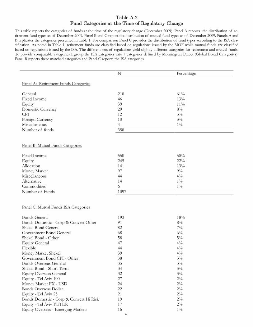
Table A.2Fund Categories at the Time of Regulatory Change

This table reports the categories of funds at the time of the regulatory change (December 2009). Panel A reports the distribution of re-tirement fund types as of December 2009. Panel B and C report the distribution of mutual fund types as of December 2009. Panels A andB replicates the categories presented in Table 1. For comparison Panel C provides the distribution of fund types according to the ISA clas-sification. As noted in Table 1, retirement funds are classified based on regulations issued by the MOF while mutual funds are classifiedbased on regulations issued by the ISA. The different sets of regulations yield slightly different categories for retirement and mutual funds.To provide comparable categories I group the ISA categories into 7 categories defined by Morningstar Direct (Global Broad Categories).Panel B reports these matched categories and Panel C reports the ISA categories.

N Percentage

Panel A: Retirement Funds Categories

General 218 61%Fixed Income 46 13%Equity 39 11%Domestic Currency 29 8%CPI 12 3%Foreign Currency 10 3%Miscellaneous 4 1%Number of funds 358

Panel B: Mutual Funds Categories

Fixed Income 550 50%Equity 245 22%Allocation 141 13%Money Market 97 9%Miscellaneous 44 4%Alternative 14 1%Commodities 6 1%Number of Funds 1097

Panel C: Mutual Funds ISA Categories

Bonds General 193 18%Bonds Domestic - Corp & Convert Other 91 8%Shekel Bond General 82 7%Government Bond General 68 6%Shekel Bond - Other 58 5%Equity General 47 4%Flexible 44 4%Money Market Shekel 39 4%Government Bond CPI - Other 38 3%Bonds Overseas General 35 3%Shekel Bond - Short Term 34 3%Equity Overseas General 32 3%Equity - Tel Aviv 100 27 2%Money Market FX - USD 24 2%Bonds Overseas Dollar 22 2%Equity - Tel Aviv 25 21 2%Bonds Domestic - Corp & Convert Hi Risk 19 2%Equity - Tel Aviv YETER 17 2%Equity Overseas - Emerging Markets 16 1%

46

Equity Overseas - Other Sectors 15 1%Government Bond CPI - Short Term 15 1%Equity Overseas - USA 13 1%Equity Overseas - Asia 11 1%Government Bond CPI - Medium Term 11 1%Equity - Real Estate 10 1%Shekel Bond - Long Term 10 1%Equity - Tel Aviv 75 9 1%Equity Overseas - Europe 9 1%Bonds Domestic - Tel Bond CPI Linked 8 1%Bonds Domestic FX - Dollar 8 1%Bonds Domestic FX - Other 8 1%Bonds Overseas Euro 7 1%Government Bond CPI - Long Term 7 1%Equity Overseas - China 6 1%Equity Overseas - Energy & Commodities 6 1%Shekel Bond - Med Term 6 1%Miscellaneous 31 3%Number of Funds 1097

47

Table A.3

Sensitivity to Losses vs. Gains

This table tests whether households are more sensitive to losses than to gains in their retirement funds. I estimate the regression of net

fund flow on lagged 1-month return . The dependent variable in Columns 1 and 3 is , the difference between flows actively ini-

tiated by households coming into and out of fund i in period t scaled by fund’s i average size. Columns 2 and 4 replace with ,

the difference between flows actively initiated by households coming into and out of fund i in period t measured in dollars. Columns 1 and 2 restrict the sample to observations with gains prior to the regulation (lagged 1-month return is positive). Columns 3 and 4 restrict the sample to retirement funds with losses prior to the regulation (lagged 1-month return is negative). The right-hand side variables are the lagged 1-month return, fund’s size, fund fixed effect and month-year fixed effects. Standard errors are robust and clustered at the fund lev-el. I report the t-statistics in brackets. *, **, and *** indicate significance at the 10%, 5%, and 1% levels, respectively.

Sensitivity to Gains Sensitivity to Losses

(1) (2) (3) (4)

0.185** 0.134** 0.284** 0.449***

[2.26] [2.20] [2.17] [3.59]

X X X X

4946 4946 2797 2797

48

REFERENCES

Anagol, S. and Gamble, K. J. (2013). Does Presenting Investment Results Asset by Asset Lower Risk Taking? Journal of Behavioral Finance 14(4), 276-300.

Barber B. and Odean T. (2008). All that glitters: the effect of attention and news on the buying behavior of individual and institutional investors. Review of Financial Studies 21, 785–818.

Barber, B. M., Odean T., and Zhu N. (2009). Systematic Noise. Journal of Financial Markets 12, 547–69.

Barberis, N. C. (2012). Thirty years of prospect theory in economics: A review and assess-ment (No. w18621). National Bureau of Economic Research.

Barberis, N. C., and Huang, M. (2001). Mental accounting, loss aversion, and individual stock returns. The Journal of Finance, 56(4), 1247-1292.

Benamar H. (2013). To See is To Know: Efficient Display of Market Data for Retail Investors. Working Paper.

Benartzi, S. and Thaler, R.H. (1995). Myopic loss aversion and the equity premium puzzle. Quarterly Journal of Economics 110, 73-92.

Benartzi, S. and Thaler, R.H. (1999). Risk aversion or myopia? Choices in repeated gambles and retirement investments. Management Science 45, 364-381.

Benartzi, S. and Thaler, R.H. (2004). Save More Tomorrow: Using Behavioral Economics to Increase Employee Savings. Journal of Political Economy 112, 164–187.

Ben Bassat, Avi. (2007). The authorities of agencies regulating capital markets in Israel and its independence. In Regulation of the Capital Market, ed. Avi Ben-Bassat, 21-74. Jerusa-lem: Israel Democracy Institute.

Ben-Rephael, A., Kandel, S., and Wohl, A. (2011). The price pressure of aggregate mutual fund flows. Journal of Financial and Quantitative Analysis,46(02), 585-603.

Beshears, J., Choi, J. J., Laibson, D., and Madrian, B. C. (2013). Simplification and sav-ing. Journal of economic behavior and organization 95, 130-145.

Beshears, J., Choi, J. J., Laibson, D., and Madrian, B. C. (2011). Does Aggregated Returns Dis-closure Increase Portfolio Risk-Taking? (No. w16868). National Bureau of Economic Re-search.

Bordalo, P., Gennaioli, N., and Shleifer, A. (2012). Salience theory of choice under risk. The Quarterly Journal of Economics 127(3), 1243-1285.

Borenstein, E., and Elkayam, D. (2014). The equity premium in a small open economy and an application to Israel. Economic Modelling, 43, 81-99.

49

Cameron, C., Gelbach, J., and Miller, D. (2011). Robust Inference with Multi-Way Clustering. Journal of Business and Economics Statistics 29 (2), 238–249.

Cameron, C., & Miller, D. (2015). A practitioner’s guide to cluster-robust inference. Journal of Human Resources, 50(2), 317-372.

Camerer, C., Issacharoff S., Loewenstein G., O’Donoghue T., and Rabin M. (2003). Regulation for Conservatives: Behavioral Economics and the Case for “Asymmetric Paternalism.” University of Pennsylvania Law Review 151, 1211–44.

Campbell, J. Y. (2006). Household finance. The Journal of Finance, 61(4), 1553-1604.

Chevalier, J. and Ellison, G. (1999). Are some mutual fund managers better than others? Cross-sectional patterns in behavior and performance. Journal of Finance 54, 875–899.

Fama, E. and MacBeth, J. (1973). Risk, return, and equilibrium: empirical tests. Journal of Po-litical Economy 71, 607–636.

Frazzini, A., Lamont, O., (2008). Dumb money: Mutual fund flows and the cross section of stock returns. Journal of Financial Economics 88, 299–322.

Frydman, C., and Rangel, A. (2013). Debiasing the disposition effect by reducing the saliency of information about a stock’s purchase prices. Working paper.

Gabaix X. (2014). A Sparsity-Based Model of Bounded Rationality. Quarterly Journal of Eco-nomics, 129(4), 1661-1710.

Gelasca, E. D., Tomasic, D., and Ebrahimi, T. (2005). Which colors best catch your eyes: a sub-jective study of color saliency. In First International Workshop on Video Processing and Quality Metrics for Consumer Electronics.

Glode, V., Hollifield, B., Kacperczyk, M., and Kogan, S. 2012. Time-Varying Predictability in Mutual Fund Returns. Working Paper, University of Pennsylvania.

Gruber, M. J., (1996). Another Puzzle: The Growth in Actively Managed Mutual Funds. Jour-nal of Finance 51, 783-810.

Hartzmark S.M. (2014). The Worst, the Best, Ignoring All the Rest: The Rank Effect and Trad-ing Behavior”. Review of Financial Studies, Forthcoming.

Hirshleifer, D. (2001). Investor psychology and asset pricing. The Journal of Finance, 56(4), 1533-1597.

Hirshleifer, D., and Teoh, S. H. (2003). Limited attention, information disclosure, and financial reporting. Journal of Accounting and Economics, 36(1), 337-386.

Hou, K., Peng, L., and Xiong Wei (2009). A tail of two anomalies: the implications of investor attention for price and earnings momentum. Working paper, Ohio State University.

Huang, J., Wei, K. D., andand Yan, H. (2007). Participation costs and the sensitivity of fund flows to past performance. The Journal of Finance, 62, 1273-1311.

50

Ippolito, R. (1992). Consumer reaction to measures of poor quality: evidence from the mutual fund industry. Journal of Law and Economics 35, 45-70.

International Monetary Fund, (2012). Israel: financial System Stability Assessment. IMF Coun-try Report No. 12/69.

Jennings M.K., and Zeigler H. (1970). The salience of American state politics. The American Political Science Review, 64, 523-535.

Jolls, C. and Sunstein C. (2006). Debiasing Through Law. Journal of Legal Studies 35, 199-241.

Kahneman, D. and Tversky, A. (1979). Prospect theory: An analysis of decision under risk. Econometrica 47, 263-291.

Kahneman, D. (1973). Attention and effort. Englewood Cliffs, NJ: Prentice-Hall.

Karlsson, N., G. Loewenstein, and D. Seppi. (2009). The “Ostrich Effect”: Selective attention to information. Journal of Risk and Uncertainty 38, 95-115.

Lim, S.S., S.H. Teoh. (2010). Limited attention. H. Kent Baker, John R. Nofsinger, eds., Behav-ioral Finance: Investors, Corporations, and Markets. John Wiley & Sons, 295–312.

Mangun, G. R. (Ed.). (2012). The neuroscience of attention: attentional control and selection. Oxford University Press.

Manzini, P., and Mariotti, M. (2014). Competing for attention: is the showiest also the best? University of St Andrews Discussion Paper No. 1403.

Odean, T. (1999). Do investors trade too much? American Economic Review 89, 1279-1298.

Osberger W. and Rohaly A.M. (2001). “Automatic detection of regions of interest in complex video sequences,” in Proceedings of Human Vision and Electronic Imaging, 361–372.

Petersen, M. (2009). Estimating Standard Errors in Finance Panel Data Sets: Comparing Ap-proaches. Review of Financial Studies 22, 435-480.

Phillips, B., Pukthuanthong, K., and Rau, P. R. (2014). Past performance may be an illusion: Performance, flows, and fees in mutual funds. Critical Finance Review, Forthcoming.

Plous, S. (1993). The Psychology of Judgment and Decision Making. Mcgraw-Hill Book Compa-ny.

Porath, Y. and Steinberg, N. (2013) Chasing Their Tails: Inflow Momentum and Yield Chasing among Provident Fund Investors in Israel. Bank of Israel Survey 86, 81-122 (in Hebrew).

Rabin, M. (2000). Risk aversion and expected‐utility theory: A calibration theorem. Economet-rica 68, 1281-1292.

Rabin, M., and Thaler, R. (2001). Anomalies: risk aversion. Journal of Economic perspectives, 219-232.

Samuelson, P.A. (1963). Risk and Uncertainty: A Fallacy of Large Numbers. Scientia 98, 108–113.

51

Sicherman, N., Loewenstein, G., Seppi, D., and Utkus, S. (2014). Financial inattention. Working Paper, Columbia University.

Sirri, E. and Tufano, P. (1998). Costly search and mutual fund flows. Journal of Finance 53, 1589–1622.

Stango, V., and Zinman, J. (2014). Limited and Varying Consumer Attention Evidence from Shocks to the Salience of Bank Overdraft Fees. Review of Financial Studies 27(4), 990-1030.

Thompson, S. B. (2011). Simple Formulas for Standard Errors that Cluster by Both Firm and Time. Journal of Financial Economics 99, 1-10.

Thaler, R. H., Tversky, A., Kahneman, D., and Schwartz, A. (1997). The effect of myopia and loss aversion on risk taking: an experimental test. Quarterly Journal of Economics 112, 647-661.

Thaler, R.H. and Sunstein C. (2008). Nudge: Improving Decisions About Health, Wealth, and Happiness. New Haven, Connecticut: Yale University Press.

Xie L. (2011). Time-varying mutual fund performance-flow sensitivity and managerial effort. Yale School of Management, Working paper.

52

Table I

Summary Statistics This table reports the summary statistics for the sample. The data span the period from January 2008 to December 2011, a total of 48 months. Panels A and B present the summary statistics for retirement funds (treated group) and mutual funds (control group) respectively. The variables presented are the mean across the sample period. 1-month return, 12-month return, and volatility are computed as value-weighted means. AUM is the average assets under management and Total AUM is the average of total assets under management for the sample period. Outflow denotes the average active flow of investments exiting funds for the sample period. Inflow denotes the average active flow of investments into funds for the sample period. All level variables are measured in millions of NIS (domestic currency) in my sample. For exposition purposes in this table I converted the averages into millions of USD. In the sample period 1 NIS was equal on average to 0.27 USD.

Mean SD Min Max

Panel A. Retirement Funds

1-Month Return (%) 0.283 2.365 -22.220 23.550 12-Month Return (%) 5.575 11.944 -55.850 147.317 AUM (mill $) 116.702 379.297 0.003 5544.819 Total AUM (mill $) 40554.410 2988.971 33112.580 44203.680 Outflow (mill $) 0.951 2.895 0 98.911 Inflow (mill $) 0.961 3.008 0 136.732 Trade (mill $) 1.911 4.421 0 138.399 Equity Exposure (%) 23.384 25.804 0 129.740 Volatility (%) 2.289 0.766 0.031 8.892

Panel B. Mutual Funds

1-month Return (%) 0.212 2.620 -85.060 90.686 12-month Return (%) 5.159 14.639 -99.954 258.045 AUM (mill $) 30.386 84.192 0.027 2617.297 Total AUM (mill $) 35998.770 5372.658 26392.380 43876.460 Outflow (mill $) 2.560 12.237 0 1177.502 Inflow (mill $) 2.603 15.160 0 685.976 Trade (mill $) 5.163 24.586 0 1274.302 Equity Exposure (%) 29.349 38.780 0 121.710 Volatility (%) 2.489 2.452 0.063 38.859

53

Table II

Fund Categories This table reports the categories of funds in my dataset. Panel A reports the average number and frequency of retire-ment fund types throughout the sample period. Retirement funds are divided into seven main categories: general, fixed income, equity, domestic currency, foreign currency, CPI and miscellaneous. These categories are based on the regulator (MOF) classification of retirement funds. The miscellaneous category includes funds that are not classified and funds classified as religious. Panel B reports the average number and frequency of mutual fund types throughout the sample period. Mutual funds are classified based on a different set of regulations by the ISA thus their categories are slightly different. To provide comparable categories I matched the ISA categories with Morningstar Direct Global Broad Cate-gories. Mutual funds are divided into seven main categories: fixed income, equity, allocation, money market, alternative, commodities, and miscellaneous. Panel B reports these matched categories. The methodology and corresponding ISA categories are described in the Appendix. This table I presents the average number and frequency of fund types across the 48 months of my sample period. The Appendix further provides a specific example of the distribution of fund types in the month of the regulatory change.

N Percentage

Panel A: Retirement Funds Categories

General 215 62% Fixed Income 42 12% Equity 38 11% Domestic Currency 27 8% CPI 11 3% Foreign Currency 10 3% Miscellaneous 4 1% Number of funds 347

Panel B: Mutual Funds Categories

Fixed Income 597 51% Equity 276 23% Allocation 140 12% Money Market 84 7% Miscellaneous 51 4% Alternative 21 2% Commodities 8 1% Number of Funds 1177

54

Table III

Fund Flow Sensitivity to Past Performance Table 3 reports the coefficient estimates from the regression of net fund flow on a set of interaction terms between 𝑃𝑃𝑃𝑃𝑃𝑃𝑡𝑡𝑡𝑡,𝑅𝑅𝐹𝐹𝑖𝑖, and 𝑟𝑟𝑖𝑖,𝑡𝑡−1 (pairwise and triple interactions). 𝐹𝐹𝐹𝐹𝑖𝑖,𝑡𝑡 denotes net fund flow measured as the difference between 𝐼𝐼𝐼𝐼𝐼𝐼𝐼𝐼𝑃𝑃𝑤𝑤𝑖𝑖,𝑡𝑡 and 𝑂𝑂𝑂𝑂𝑡𝑡𝐼𝐼𝐼𝐼𝑃𝑃𝑤𝑤𝑖𝑖,𝑡𝑡. 𝐹𝐹𝐹𝐹𝐹𝐹𝑖𝑖,𝑡𝑡 denotes net fund flow measured as the difference between (𝐼𝐼𝐼𝐼𝐼𝐼𝐼𝐼𝑃𝑃𝑤𝑤𝑖𝑖,𝑡𝑡 + 𝐷𝐷𝐷𝐷𝐷𝐷𝑃𝑃𝑃𝑃𝐷𝐷𝑡𝑡𝑖𝑖,𝑡𝑡) and (𝑂𝑂𝑂𝑂𝑡𝑡𝐼𝐼𝐼𝐼𝑃𝑃𝑤𝑤𝑖𝑖,𝑡𝑡 + 𝑊𝑊𝐷𝐷𝑡𝑡ℎ𝑑𝑑𝑟𝑟𝑑𝑑𝑤𝑤𝑑𝑑𝐼𝐼𝑖𝑖,𝑡𝑡). 𝑀𝑀𝑀𝑀𝑡𝑡𝑆𝑆𝑖𝑖,𝑡𝑡 denotes the change in the percentage market share held by fund i from period t-1 to period t times 100. 𝐹𝐹𝐹𝐹𝑆𝑆𝑖𝑖,𝑡𝑡 and 𝐹𝐹𝐹𝐹𝐹𝐹𝑆𝑆𝑖𝑖,𝑡𝑡 denote, respectively, 𝐹𝐹𝐹𝐹𝑖𝑖,𝑡𝑡 and 𝐹𝐹𝐹𝐹𝐹𝐹𝑖𝑖,𝑡𝑡 scaled by average fund size. 𝑟𝑟𝑖𝑖,𝑡𝑡−1 is the lagged 1-month return. 𝑃𝑃𝑃𝑃𝑃𝑃𝑡𝑡𝑡𝑡 is an indicator variable for whether the observation occurred after the regulation. 𝑅𝑅𝐹𝐹𝑖𝑖 is an indicator variable for whether the fund is a retirement fund. 𝐶𝐶𝑃𝑃𝐼𝐼𝑡𝑡𝑟𝑟𝑃𝑃𝐼𝐼𝑃𝑃 are controls for fund size, fund fixed effects and month-year fixed effects. Net fund flow data are winsorized at the upper and lower 2% level. The coefficients of interest are the coefficients on the triple interaction terms. Standard errors are robust and clustered at the fund level. I report the t-statistics in brackets. ***, **, and * denote the significance at 1%, 5%, and 10%, respectively.

(1) (2) (3) (4) (5)

𝐹𝐹𝐹𝐹𝑖𝑖,𝑡𝑡 𝐹𝐹𝐹𝐹𝐹𝐹𝑖𝑖𝑡𝑡 𝑀𝑀𝑀𝑀𝑡𝑡𝑆𝑆𝑖𝑖,𝑡𝑡 𝐹𝐹𝐹𝐹𝑆𝑆𝑖𝑖,𝑡𝑡 𝐹𝐹𝐹𝐹𝐹𝐹𝑆𝑆𝑖𝑖,𝑡𝑡

𝑃𝑃𝑃𝑃𝑃𝑃𝑡𝑡𝑡𝑡 × 𝑅𝑅𝐹𝐹𝑖𝑖 -0.774 -0.446 -0.0657 -0.817*** -0.811*** [-0.76] [-0.42] [-0.55] [-2.78] [-2.72]

𝑟𝑟𝑖𝑖,𝑡𝑡−1 0.239*** 0.233*** 0.0349*** 0.161*** 0.160*** [2.93] [2.85] [3.89] [5.41] [5.38]

𝑟𝑟𝑖𝑖,𝑡𝑡−1 × 𝑅𝑅𝐹𝐹𝑖𝑖 0.316** 0.479*** 0.0492*** -0.125*** -0.102*** [2.35] [3.02] [3.22] [-3.80] [-3.01]

𝑟𝑟𝑖𝑖,𝑡𝑡−1 × 𝑃𝑃𝑃𝑃𝑃𝑃𝑡𝑡𝑡𝑡 0.135 0.138 -0.00356 0.474*** 0.475*** [1.48] [1.51] [-0.40] [7.47] [7.48]

𝑟𝑟𝑖𝑖,𝑡𝑡−1 × 𝑃𝑃𝑃𝑃𝑃𝑃𝑡𝑡𝑡𝑡 × 𝑅𝑅𝐹𝐹𝑖𝑖 -0.608*** -0.713*** -0.0574*** -0.406*** -0.407*** [-4.45] [-4.70] [-3.54] [-5.09] [-5.07]

𝐶𝐶𝑃𝑃𝐼𝐼𝑡𝑡𝑟𝑟𝑃𝑃𝐼𝐼𝑃𝑃 X X X X X

𝑁𝑁 73074 73074 73074 73074 73074

55

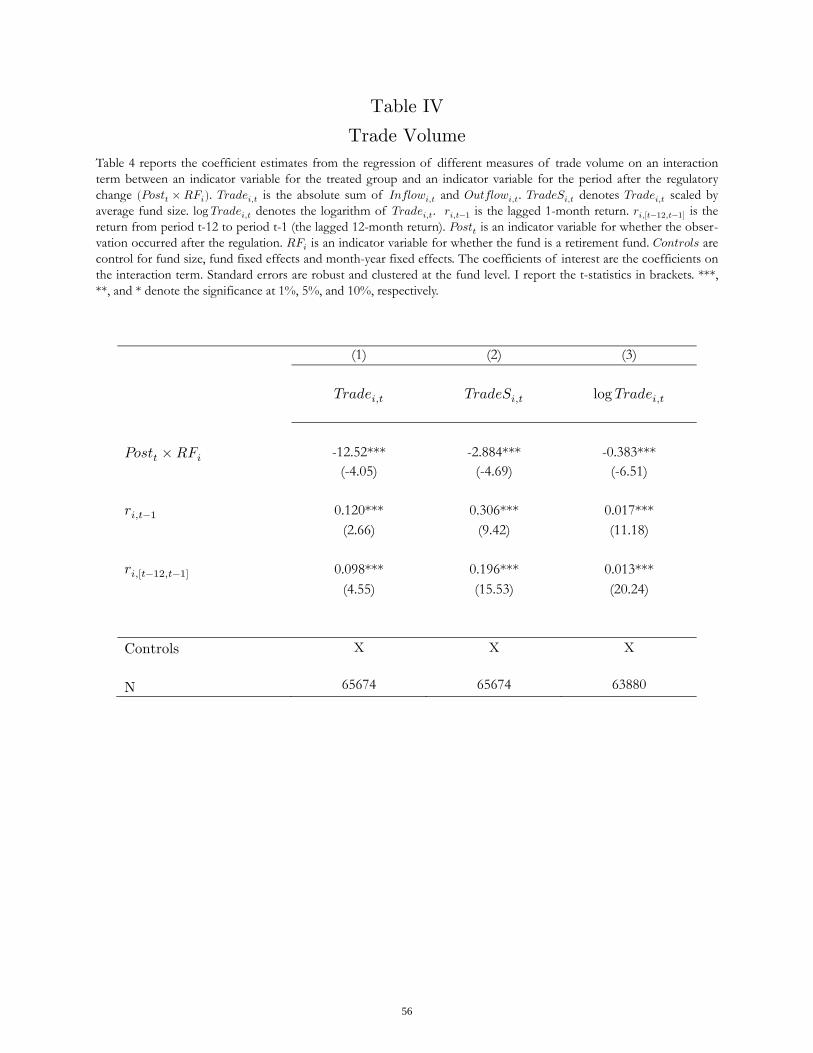
Table IV

Trade Volume

Table 4 reports the coefficient estimates from the regression of different measures of trade volume on an interaction term between an indicator variable for the treated group and an indicator variable for the period after the regulatory change (𝑃𝑜𝑠𝑡𝑡 × 𝑅𝐹𝑖). 𝑇𝑟𝑎𝑑𝑒𝑖,𝑡 is the absolute sum of 𝐼𝑛𝑓𝑙𝑜𝑤𝑖,𝑡 and 𝑂𝑢𝑡𝑓𝑙𝑜𝑤𝑖,𝑡. 𝑇𝑟𝑎𝑑𝑒𝑆𝑖,𝑡 denotes 𝑇𝑟𝑎𝑑𝑒𝑖,𝑡 scaled by average fund size. log 𝑇𝑟𝑎𝑑𝑒𝑖,𝑡 denotes the logarithm of 𝑇𝑟𝑎𝑑𝑒𝑖,𝑡. 𝑟𝑖,𝑡−1 is the lagged 1-month return. 𝑟𝑖,[𝑡−12,𝑡−1] is the return from period t-12 to period t-1 (the lagged 12-month return). 𝑃𝑜𝑠𝑡𝑡 is an indicator variable for whether the obser-vation occurred after the regulation. 𝑅𝐹𝑖 is an indicator variable for whether the fund is a retirement fund. 𝐶𝑜𝑛𝑡𝑟𝑜𝑙𝑠 are control for fund size, fund fixed effects and month-year fixed effects. The coefficients of interest are the coefficients on the interaction term. Standard errors are robust and clustered at the fund level. I report the t-statistics in brackets. ***, **, and * denote the significance at 1%, 5%, and 10%, respectively.

(1) (2) (3)

𝑇𝑟𝑎𝑑𝑒𝑖,𝑡 𝑇𝑟𝑎𝑑𝑒𝑆𝑖,𝑡 log 𝑇𝑟𝑎𝑑𝑒𝑖,𝑡

𝑃𝑜𝑠𝑡𝑡 × 𝑅𝐹𝑖 -12.52*** -2.884*** -0.383***(-4.05) (-4.69) (-6.51)

𝑟𝑖,𝑡−1 0.120*** 0.306*** 0.017***(2.66) (9.42) (11.18)

𝑟𝑖,[𝑡−12,𝑡−1] 0.098*** 0.196*** 0.013***(4.55) (15.53) (20.24)

Controls X X X

N 65674 65674 63880

56

Table V

Risk Allocation: Net Fund Flow This table reports the coefficient estimates from the regression of net fund flow on a set of interactions term using two different measures of fund risk profile. The dependent variable in Columns 1 and 3 is 𝐹𝐹𝐹𝐹𝑆𝑆𝑖𝑖,𝑡𝑡, the difference between flows actively initiated by households into and out of fund i in period t scaled by fund average size. Columns 2 and 4 replace 𝐹𝐹𝐹𝐹𝑆𝑆𝑖𝑖,𝑡𝑡 with 𝐹𝐹𝐹𝐹𝑖𝑖,𝑡𝑡, the difference between flows actively initiated by households into and out of fund i in period t measured in dollars. The two risk measures, fund’s volatility (𝐹𝐹𝑃𝑃𝐼𝐼𝑖𝑖) and fund’s equity exposure (𝐸𝐸𝐸𝐸𝑖𝑖), proxy for fund i risk profile. 𝐸𝐸𝐸𝐸𝑖𝑖 denotes fund’s i average equity exposure for the period prior to the regulation. Both retirement and mutual funds are required to report monthly their equity exposures starting 2008. Equity exposure is computed as the percentage of fund’s AUM invested in equities and equity derivatives. I collected the equity exposure data from the MOF and TASE websites. 𝐹𝐹𝑃𝑃𝐼𝐼𝑖𝑖 is an alternative proxy for fund i's risk profile. 𝐹𝐹𝑃𝑃𝐼𝐼𝑖𝑖 equals the average standard deviation of fund i’s monthly returns prior to the regulation. I compute the standard deviation mirroring the standard deviation measure presented to households. For each fund i in every period t, I compute the standard deviation of 1-month re-turns for the previous 36 months window. I then average these standard deviations for each fund i for the period prior to the regulation and report it as 𝐹𝐹𝑃𝑃𝐼𝐼𝑖𝑖. 𝑃𝑃𝑃𝑃𝑃𝑃𝑡𝑡𝑡𝑡 is an indicator variable for whether the observation occurred after the regula-tion. 𝑅𝑅𝐹𝐹𝑖𝑖 is an indicator variable for whether the fund is a retirement fund. My independent variables include all possible interaction terms between 𝑃𝑃𝑃𝑃𝑃𝑃𝑡𝑡𝑡𝑡,𝑅𝑅𝐹𝐹𝑖𝑖, and the risk measure used (pairwise and triple interactions). The main coefficient of interest is the coefficient on the triple interaction term (𝛽𝛽3). It represents the change in fund flow allocation to riskier retirement funds following the regulation compared to the control group. 𝐶𝐶𝑃𝑃𝐼𝐼𝑡𝑡𝑟𝑟𝑃𝑃𝐼𝐼𝑃𝑃 are controls for fund size, lagged 1-month return, past 12-month return, fund fixed effects and month-year fixed effects. Standard errors are robust and clustered at the fund level. I report the t-statistics in brackets. ***, **, and * denote the significance at 1%, 5%, and 10%, respectively.

(1) (2) (3) (4)

𝐹𝐹𝐹𝐹𝑆𝑆𝑖𝑖,𝑡𝑡 𝐹𝐹𝐹𝐹𝑖𝑖,𝑡𝑡 𝐹𝐹𝐹𝐹𝑆𝑆𝑖𝑖,𝑡𝑡 𝐹𝐹𝐹𝐹𝑖𝑖,𝑡𝑡

𝑃𝑃𝑃𝑃𝑃𝑃𝑡𝑡𝑡𝑡 × 𝑅𝑅𝐹𝐹𝑖𝑖 -0.0257*** -1.135 -0.0169*** -0.483

[-4.64] [-1.31] [-5.03] [-0.96]

𝑃𝑃𝑃𝑃𝑃𝑃𝑡𝑡𝑡𝑡 × 𝑅𝑅𝐷𝐷𝑃𝑃𝑀𝑀𝑀𝑀𝐷𝐷𝑑𝑑𝑃𝑃𝑂𝑂𝑟𝑟𝐷𝐷𝑖𝑖 -0.00225** 0.0762 -0.000179*** -0.0124***

[-2.55] [0.75] [-3.33] [-2.63]

𝑃𝑃𝑃𝑃𝑃𝑃𝑡𝑡𝑡𝑡 × 𝑅𝑅𝐷𝐷𝑃𝑃𝑀𝑀𝑀𝑀𝐷𝐷𝑑𝑑𝑃𝑃𝑂𝑂𝑟𝑟𝐷𝐷𝑖𝑖 × 𝑅𝑅𝐹𝐹𝑖𝑖 0.00572*** 0.772*** 0.000222*** 0.0317***

[3.27] [2.91] [2.60] [2.81]

𝑅𝑅𝐷𝐷𝑃𝑃𝑀𝑀 𝑀𝑀𝐷𝐷𝑑𝑑𝑃𝑃𝑂𝑂𝑟𝑟𝐷𝐷 𝑇𝑇𝑇𝑇𝐷𝐷𝐷𝐷 Volatility Volatility Equity Equity

𝐶𝐶𝑃𝑃𝐼𝐼𝑡𝑡𝑟𝑟𝑃𝑃𝐼𝐼𝑃𝑃 X X X X

𝑁𝑁 48483 48483 52527 52527

57

Table VI

Risk Allocation: Inflow vs. Outflow This table tests whether flows in and out of risky retirement funds changed following the regulation. Panel A uses 𝐹𝐹𝑃𝑃𝐼𝐼𝑖𝑖 as proxy for fund risk profile. Panel B replaces 𝐹𝐹𝑃𝑃𝐼𝐼𝑖𝑖 with 𝐸𝐸𝐸𝐸𝑖𝑖 as the proxy for fund risk profile. Both risk measures are as described in Table 5. The dependent variables in Columns 1 and 2 are, respectively, 𝐿𝐿𝑃𝑃𝐿𝐿�𝐼𝐼𝑁𝑁𝑆𝑆𝑖𝑖,𝑡𝑡�, the logarithm of flows into fund i in period t scaled and 𝐿𝐿𝑃𝑃𝐿𝐿�𝐼𝐼𝑁𝑁𝑖𝑖,𝑡𝑡�, the logarithm of flows into fund i in period t. The dependent variables in Columns 3 and 4 are, respectively, 𝐿𝐿𝑃𝑃𝐿𝐿�𝑂𝑂𝑂𝑂𝑇𝑇𝑆𝑆𝑖𝑖,𝑡𝑡�, the logarithm of flows out of fund i in period t scaled and 𝐿𝐿𝑃𝑃𝐿𝐿�𝑂𝑂𝑂𝑂𝑇𝑇𝑖𝑖,𝑡𝑡�, the logarithm of flows out of fund i in period t. 𝑃𝑃𝑃𝑃𝑃𝑃𝑡𝑡𝑡𝑡 is an indicator variable for whether the observation occurred after the regulation. 𝑅𝑅𝐹𝐹𝑖𝑖 is an indicator variable for whether the fund is a retirement fund. My independent variables include all possible interactions terms between 𝑃𝑃𝑃𝑃𝑃𝑃𝑡𝑡𝑡𝑡,𝑅𝑅𝐹𝐹𝑖𝑖, and the risk measure used (pairwise and triple inter-actions). The main coefficients of interest are the coefficients of the triple interaction terms. 𝐶𝐶𝑃𝑃𝐼𝐼𝑡𝑡𝑟𝑟𝑃𝑃𝐼𝐼𝑃𝑃 are controls for fund size, past 1-month return, past 12-month return, fund fixed effects and month-year fixed effects. Standard errors are robust and clustered at the fund level. I report the t-statistics in brackets. ***, **, and * denote the significance at 1%, 5%, and 10%, respectively.

Panel A: Volatility as risk measure

(1) (2) (3) (4)

Log�𝐼𝐼𝑁𝑁𝑆𝑆𝑖𝑖,𝑡𝑡� Log�𝐼𝐼𝑁𝑁𝑖𝑖,𝑡𝑡� Log�𝑂𝑂𝑂𝑂𝑇𝑇𝑆𝑆𝑖𝑖,𝑡𝑡� Log�𝑂𝑂𝑂𝑂𝑇𝑇𝑖𝑖,𝑡𝑡�

𝑃𝑃𝑃𝑃𝑃𝑃𝑡𝑡𝑡𝑡 × 𝑅𝑅𝐹𝐹𝑖𝑖 -0.0330*** -0.786*** -0.00638* -0.0194 [-6.61] [-4.79] [-1.95] [-0.18]

𝑃𝑃𝑃𝑃𝑃𝑃𝑡𝑡𝑡𝑡 × 𝐹𝐹𝑃𝑃𝐼𝐼𝑖𝑖 -0.00261*** -0.0517*** 0.000786 0.0468*** [-3.10] [-3.78] [1.16] [4.57]

𝑃𝑃𝑃𝑃𝑃𝑃𝑡𝑡𝑡𝑡 × 𝐹𝐹𝑃𝑃𝐼𝐼𝑖𝑖 × 𝑅𝑅𝐹𝐹𝑖𝑖 0.00537*** 0.152*** -0.000831 -0.0748* [3.03] [2.65] [-0.82] [-1.86]

𝐶𝐶𝑃𝑃𝐼𝐼𝑡𝑡𝑟𝑟𝑃𝑃𝐼𝐼𝑃𝑃 X X X X

𝑁𝑁 48483 44729 48483 46548

Panel B: Equity Exposure as risk measure

(1) (2) (3) (4)

Log�𝐼𝐼𝑁𝑁𝑆𝑆𝑖𝑖,𝑡𝑡� Log�𝐼𝐼𝑁𝑁𝑖𝑖,𝑡𝑡� Log�𝑂𝑂𝑂𝑂𝑇𝑇𝑆𝑆𝑖𝑖,𝑡𝑡� Log�𝑂𝑂𝑂𝑂𝑇𝑇𝑖𝑖,𝑡𝑡�

𝑃𝑃𝑃𝑃𝑃𝑃𝑡𝑡𝑡𝑡 × 𝑅𝑅𝐹𝐹𝑖𝑖 -0.0241*** -0.570*** -0.00802*** -0.153** [-6.70] [-4.95] [-2.81] [-2.00]

𝑃𝑃𝑃𝑃𝑃𝑃𝑡𝑡𝑡𝑡 × 𝐸𝐸𝐸𝐸𝑖𝑖 -0.0000956 -0.00186 0.0000782 0.00267*** [-1.64] [-1.57] [1.54] [3.12]

𝑃𝑃𝑃𝑃𝑃𝑃𝑡𝑡𝑡𝑡 × 𝐸𝐸𝐸𝐸𝑖𝑖 × 𝑅𝑅𝐹𝐹𝑖𝑖 0.000224** 0.00761** -0.0000252 -0.00231 [2.17] [2.39] [-0.36] [-1.12]

𝐶𝐶𝑃𝑃𝐼𝐼𝑡𝑡𝑟𝑟𝑃𝑃𝐼𝐼𝑃𝑃 X X X X 𝑁𝑁 52527 48649 52527 50463

58

Table VII

Absolute and Relative Salience Table 7 reports the coefficient estimate from the regression of net fund flow on two sets of interaction terms. The first includes all interactions between 𝑃𝑃𝑃𝑃𝑃𝑃𝑡𝑡𝑡𝑡, 𝑅𝑅𝐹𝐹𝑖𝑖, and 𝑟𝑟𝑖𝑖,𝑡𝑡−1 (pairwise and triple interactions). The second includes all interac-tions between 𝑃𝑃𝑃𝑃𝑃𝑃𝑡𝑡𝑡𝑡,𝑅𝑅𝐹𝐹𝑖𝑖, and 𝑟𝑟𝑖𝑖,[𝑡𝑡−12𝑡𝑡−1] (pairwise and triple interactions). 𝐹𝐹𝐹𝐹𝑖𝑖,𝑡𝑡 denotes net fund flow measured as the difference between 𝐼𝐼𝐼𝐼𝐼𝐼𝐼𝐼𝑃𝑃𝑤𝑤𝑖𝑖,𝑡𝑡 and 𝑂𝑂𝑂𝑂𝑡𝑡𝐼𝐼𝐼𝐼𝑃𝑃𝑤𝑤𝑖𝑖,𝑡𝑡. 𝐹𝐹𝐹𝐹𝐹𝐹𝑖𝑖,𝑡𝑡 denotes net fund flow measured as the difference between �𝐼𝐼𝐼𝐼𝐼𝐼𝐼𝐼𝑃𝑃𝑤𝑤𝑖𝑖,𝑡𝑡 + 𝐷𝐷𝐷𝐷𝐷𝐷𝑃𝑃𝑃𝑃𝐷𝐷𝑡𝑡𝑖𝑖,𝑡𝑡� and �𝑂𝑂𝑂𝑂𝑡𝑡𝐼𝐼𝐼𝐼𝑃𝑃𝑤𝑤𝑖𝑖,𝑡𝑡 + 𝑊𝑊𝐷𝐷𝑡𝑡ℎ𝑑𝑑𝑟𝑟𝑑𝑑𝑤𝑤𝑑𝑑𝐼𝐼𝑖𝑖,𝑡𝑡�. 𝑀𝑀𝑀𝑀𝑡𝑡𝑆𝑆𝑖𝑖,𝑡𝑡 denotes the change in the percentage market share held by fund i from period t-1 to period t times 100. 𝐹𝐹𝐹𝐹𝑆𝑆𝑖𝑖,𝑡𝑡 and 𝐹𝐹𝐹𝐹𝐹𝐹𝑆𝑆𝑖𝑖,𝑡𝑡 denote 𝐹𝐹𝐹𝐹𝑖𝑖,𝑡𝑡 and 𝐹𝐹𝐹𝐹𝐹𝐹𝑖𝑖,𝑡𝑡 scaled by fund size. 𝑟𝑟𝑖𝑖,𝑡𝑡−1 is the lagged 1-month return. 𝑟𝑟𝑖𝑖,[𝑡𝑡−12𝑡𝑡−1] is the return from period t-12 to period t-1 (the lagged 12-month return). 𝑃𝑃𝑃𝑃𝑃𝑃𝑡𝑡𝑡𝑡 is an indicator variable for whether the observation occurred after the regulation. 𝑅𝑅𝐹𝐹𝑖𝑖 is an indicator variable for whether the fund is a retirement fund. 𝐶𝐶𝑃𝑃𝐼𝐼𝑡𝑡𝑟𝑟𝑃𝑃𝐼𝐼𝑃𝑃 are control for fund size, fund fixed effects and month-year fixed ef-fects. For the treated group (retirement funds) I obtained the return data from the MOF website. I additionally conduct-ed tests to confirm the values used for the 12-month return conform to the values used for monthly returns. For the control group (mutual funds) I obtained the return data from Praedicta (an Israeli data vendor). Net fund flow data are winsorized at the upper and lower 2% level. The coefficients of interest are the coefficients on the triple interaction terms. Standard errors are robust and clustered at the fund level. I report the t-statistics in brackets. ***, **, and * denote the significance at 1%, 5%, and 10%, respectively.

(1) (2) (3) (4) (5) 𝐹𝐹𝐹𝐹𝑖𝑖,𝑡𝑡 𝐹𝐹𝐹𝐹𝐹𝐹𝑖𝑖𝑡𝑡 𝑀𝑀𝑀𝑀𝑡𝑡𝑆𝑆𝑖𝑖,𝑡𝑡 𝐹𝐹𝐹𝐹𝑆𝑆𝑖𝑖,𝑡𝑡 𝐹𝐹𝐹𝐹𝐹𝐹𝑆𝑆𝑖𝑖,𝑡𝑡

𝑃𝑃𝑃𝑃𝑃𝑃𝑡𝑡𝑡𝑡 × 𝑅𝑅𝐹𝐹𝑖𝑖 -0.417 -0.292 -0.112 -1.371*** -1.418*** [-0.36] [-0.25] [-0.84] [-4.03] [-4.06]

𝑟𝑟𝑖𝑖,𝑡𝑡−1 0.119** 0.114* 0.0252*** 0.121*** 0.120*** [2.01] [1.92] [4.00] [4.15] [4.13]

𝑟𝑟𝑖𝑖,𝑡𝑡−1 × 𝑅𝑅𝐹𝐹𝑖𝑖 0.115 0.286** 0.0296** -0.256*** -0.233*** [1.00] [1.99] [2.28] [-7.49] [-6.79]

𝑟𝑟𝑖𝑖,𝑡𝑡−1 × 𝑃𝑃𝑃𝑃𝑃𝑃𝑡𝑡𝑡𝑡 0.193*** 0.196*** -0.000860 0.418*** 0.419*** [2.63] [2.67] [-0.13] [7.56] [7.56]

𝑟𝑟𝑖𝑖,𝑡𝑡−1 × 𝑃𝑃𝑃𝑃𝑃𝑃𝑡𝑡𝑡𝑡 × 𝑅𝑅𝐹𝐹𝑖𝑖 -0.335*** -0.483*** -0.0367*** -0.189** -0.204*** [-2.80] [-3.38] [-2.58] [-2.52] [-2.71]

𝑟𝑟𝑖𝑖,[𝑡𝑡−12,𝑡𝑡−1] 0.0365* 0.0334* -0.00176 -0.000112 -0.000617 [1.86] [1.69] [-0.89] [-0.01] [-0.07]

𝑟𝑟𝑖𝑖,[𝑡𝑡−12,𝑡𝑡−1] × 𝑅𝑅𝐹𝐹𝑖𝑖 0.164*** 0.181*** 0.0147*** 0.154*** 0.156*** [4.11] [4.33] [2.79] [9.34] [9.10]

𝑟𝑟𝑖𝑖,[𝑡𝑡−12,𝑡𝑡−1] × 𝑃𝑃𝑃𝑃𝑃𝑃𝑡𝑡𝑡𝑡 -0.00311 -0.000840 0.00608*** 0.0418*** 0.0422*** [-0.14] [-0.04] [2.78] [3.24] [3.27]

𝑟𝑟𝑖𝑖,[𝑡𝑡−12,𝑡𝑡−1] × 𝑃𝑃𝑃𝑃𝑃𝑃𝑡𝑡𝑡𝑡 × 𝑅𝑅𝐹𝐹𝑖𝑖 -0.197*** -0.197*** -0.0141** -0.194*** -0.192*** [-4.48] [-4.40] [-2.40] [-9.83] [-9.32]

𝐶𝐶𝑃𝑃𝐼𝐼𝑡𝑡𝑟𝑟𝑃𝑃𝐼𝐼𝑃𝑃 X X X X X

𝑁𝑁 65720 65720 65720 65720 65720

59

Table VIII

Robustness Tests

Panels A, B and C replicate the estimates from Tables 3, 4, and 7 respectively clustering standard errors at the fund and month-year levels. All variables are defined as noted in Tables 3, 4, and 7. The coefficients of interest are the coefficients on the triple interaction terms. Standard errors are robust and clustered at the fund and month-year levels. I report the t-statistics in brackets. ***, **, and * denote the significance at 1%, 5%, and 10%, respectively.

Panel A (1) (2) (3) (4) (5)

𝐹𝐹𝑆𝑖,𝑡 𝐹𝐹𝑉𝑆𝑖𝑡 𝑀𝑘𝑡𝑆𝑖,𝑡 𝐹𝐹𝑖,𝑡 𝐹𝐹𝑉𝑖,𝑡

𝑃𝑜𝑠𝑡𝑡 × 𝑅𝐹𝑖 -0.774 -0.446 -0.0657 -0.817 -0.811[-0.60] [-0.37] [-0.48] [-0.85] [-0.84]

𝑟𝑖,𝑡−1 0.239*** 0.233*** 0.0349*** 0.161*** 0.160***[2.94] [2.84] [3.22] [3.57] [3.51]

𝑟𝑖,𝑡−1 × 𝑅𝐹𝑖 0.316** 0.479*** 0.0492*** -0.125 -0.102[2.13] [2.70] [2.87] [-1.11] [-0.87]

𝑟𝑖,𝑡−1 × 𝑃𝑜𝑠𝑡𝑡 0.135 0.138 -0.00356 0.474*** 0.475***[1.16] [1.18] [-0.27] [2.71] [2.73]

𝑟𝑖,𝑡−1 × 𝑃𝑜𝑠𝑡𝑡 × 𝑅𝐹𝑖 -0.608*** -0.713*** -0.0574*** -0.406** -0.407**[-3.40] [-3.76] [-3.05] [-2.22] [-2.23]

𝐶𝑜𝑛𝑡𝑟𝑜𝑙𝑠 X X X X X

𝑁 73074 73074 73074 73074 73074

Panel B (1) (2) (3)

𝑇𝑟𝑎𝑑𝑒𝑖,𝑡 𝑇𝑟𝑎𝑑𝑒𝑆𝑖,𝑡 log 𝑇𝑟𝑎𝑑𝑒𝑖,𝑡

𝑃𝑜𝑠𝑡𝑡 × 𝑅𝐹𝑖 -12.52*** -2.884** -0.383***[-3.50] [-2.45] [-3.45]

𝑟𝑖,𝑡−1 0.120** 0.306*** 0.017***[1.99] [4.62] [5.58]

𝑟𝑖,[𝑡−12,𝑡−1] 0.098*** 0.196*** 0.013***

[3.69] [9.56] [7.70]

𝐶𝑜𝑛𝑡𝑟𝑜𝑙𝑠 X X X

𝑁 65674 65674 63880

60

Panel C

(1) (2) (3) (4) (5) 𝐹𝐹𝐹𝐹𝑖𝑖,𝑡𝑡 𝐹𝐹𝐹𝐹𝐹𝐹𝑖𝑖,𝑡𝑡 𝑀𝑀𝑀𝑀𝑡𝑡𝑆𝑆𝑖𝑖,𝑡𝑡 𝐹𝐹𝐹𝐹𝑆𝑆𝑖𝑖,𝑡𝑡 𝐹𝐹𝐹𝐹𝐹𝐹𝑆𝑆𝑖𝑖,𝑡𝑡

𝑃𝑃𝑃𝑃𝑃𝑃𝑡𝑡𝑡𝑡 × 𝑅𝑅𝐹𝐹𝑖𝑖 -0.417 -0.292 -0.112 -1.371 -1.418 [-0.29] [-0.22] [-0.78] [-1.15] [-1.19]

𝑟𝑟𝑖𝑖,𝑡𝑡−1 0.119* 0.114 0.0252*** 0.121** 0.120** [1.72] [1.64] [2.90] [2.41] [2.39]

𝑟𝑟𝑖𝑖,𝑡𝑡−1 × 𝑅𝑅𝐹𝐹𝑖𝑖 0.115 0.286* 0.0296** -0.256*** -0.233*** [0.86] [1.86] [2.00] [-3.59] [-3.25]

𝑟𝑟𝑖𝑖,𝑡𝑡−1 × 𝑃𝑃𝑃𝑃𝑃𝑃𝑡𝑡𝑡𝑡 0.193* 0.196* -0.000860 0.418*** 0.419*** [1.79] [1.82] [-0.07] [2.75] [2.76]

𝑟𝑟𝑖𝑖,𝑡𝑡−1 × 𝑃𝑃𝑃𝑃𝑃𝑃𝑡𝑡𝑡𝑡 × 𝑅𝑅𝐹𝐹𝑖𝑖 -0.335* -0.483*** -0.0367** -0.189 -0.204 [-1.89] [-2.65] [-2.03] [-1.26] [-1.36]

𝑟𝑟𝑖𝑖,[𝑡𝑡−12,𝑡𝑡−1] 0.0365 0.0334 -0.00176 -0.000112 -0.000617 [1.32] [1.19] [-0.54] [-0.00] [-0.03]

𝑟𝑟𝑖𝑖,[𝑡𝑡−12,𝑡𝑡−1] × 𝑅𝑅𝐹𝐹𝑖𝑖 0.164*** 0.181*** 0.0147** 0.154** 0.156** [2.60] [2.85] [2.32] [2.23] [2.26]

𝑟𝑟𝑖𝑖,[𝑡𝑡−12,𝑡𝑡−1] × 𝑃𝑃𝑃𝑃𝑃𝑃𝑡𝑡𝑡𝑡 -0.00311 -0.000840 0.00608 0.0418 0.0422 [-0.08] [-0.02] [1.41] [1.15] [1.16]

𝑟𝑟𝑖𝑖,[𝑡𝑡−12,𝑡𝑡−1] × 𝑃𝑃𝑃𝑃𝑃𝑃𝑡𝑡𝑡𝑡 × 𝑅𝑅𝐹𝐹𝑖𝑖 -0.197*** -0.197*** -0.0141** -0.194*** -0.192** [-2.93] [-3.00] [-2.06] [-2.58] [-2.54]

𝐶𝐶𝑃𝑃𝐼𝐼𝑡𝑡𝑟𝑟𝑃𝑃𝐼𝐼𝑃𝑃 X X X X X

𝑁𝑁 65720 65720 65720 65720 65720

61

Table IX

Robustness Tests Panels A and B replicate the estimates from Tables 3 and 7, respectively, without including time fixed effects and cluster-ing standard errors at the fund and month-year levels. 𝐹𝐹𝐹𝐹𝑖𝑖,𝑡𝑡 denotes net fund flow measured as the difference between 𝐼𝐼𝐼𝐼𝐼𝐼𝐼𝐼𝑃𝑃𝑤𝑤𝑖𝑖,𝑡𝑡 and 𝑂𝑂𝑂𝑂𝑡𝑡𝐼𝐼𝐼𝐼𝑃𝑃𝑤𝑤𝑖𝑖,𝑡𝑡. 𝐹𝐹𝐹𝐹𝐹𝐹𝑖𝑖,𝑡𝑡 denotes net fund flow measured as the difference between (𝐼𝐼𝐼𝐼𝐼𝐼𝐼𝐼𝑃𝑃𝑤𝑤𝑖𝑖,𝑡𝑡 + 𝐷𝐷𝐷𝐷𝐷𝐷𝑃𝑃𝑃𝑃𝐷𝐷𝑡𝑡𝑖𝑖,𝑡𝑡) and (𝑂𝑂𝑂𝑂𝑡𝑡𝐼𝐼𝐼𝐼𝑃𝑃𝑤𝑤𝑖𝑖,𝑡𝑡 + 𝑊𝑊𝐷𝐷𝑡𝑡ℎ𝑑𝑑𝑟𝑟𝑑𝑑𝑤𝑤𝑑𝑑𝐼𝐼𝑖𝑖,𝑡𝑡). 𝐹𝐹𝐹𝐹𝑆𝑆𝑖𝑖,𝑡𝑡 and 𝐹𝐹𝐹𝐹𝐹𝐹𝑆𝑆𝑖𝑖,𝑡𝑡 denote 𝐹𝐹𝐹𝐹𝑖𝑖,𝑡𝑡 and 𝐹𝐹𝐹𝐹𝐹𝐹𝑖𝑖,𝑡𝑡 scaled by average fund’s size respectively. 𝑀𝑀𝑀𝑀𝑡𝑡𝑆𝑆𝑖𝑖,𝑡𝑡 denotes the change in the percentage market share held by fund i from period t-1 times 100. 𝑟𝑟𝑖𝑖,𝑡𝑡−1 is the lagged month 1-month return. 𝑟𝑟𝑖𝑖,[𝑡𝑡−12,𝑡𝑡−1] is the return from period t-12 to period t-1 (the lagged 12-month return). 𝑃𝑃𝑃𝑃𝑃𝑃𝑡𝑡𝑡𝑡 is an indicator variable for whether the observation occurred after the regulation. 𝑅𝑅𝐹𝐹𝑖𝑖 is an indicator variable for whether the fund is a retirement fund. 𝐶𝐶𝑃𝑃𝐼𝐼𝑡𝑡𝑟𝑟𝑃𝑃𝐼𝐼𝑃𝑃 are controls for fund’s size, and fund fixed effects. Net fund flow data are winsorized at the upper and lower 2% level. The coefficients of interest are the coefficients on the triple interaction terms. Standard errors are robust and clustered at the fund and month-year levels. I report the t-statistics in brackets. ***, **, and * de-note the significance at 1%, 5%, and 10%, respectively.

Panel A (1) (2) (3) (4) (5)

𝐹𝐹𝐹𝐹𝑆𝑆𝑖𝑖,𝑡𝑡 𝐹𝐹𝐹𝐹𝐹𝐹𝑆𝑆𝑖𝑖𝑡𝑡 𝑀𝑀𝑀𝑀𝑡𝑡𝑆𝑆𝑖𝑖,𝑡𝑡 𝐹𝐹𝐹𝐹𝑖𝑖,𝑡𝑡 𝐹𝐹𝐹𝐹𝐹𝐹𝑖𝑖,𝑡𝑡

𝑃𝑃𝑃𝑃𝑃𝑃𝑡𝑡𝑡𝑡 0.0809 -0.848 -0.129*** 0.0817 -0.840 [0.09] [-1.22] [-2.74] [0.10] [-1.21]

𝑃𝑃𝑃𝑃𝑃𝑃𝑡𝑡𝑡𝑡 × 𝑅𝑅𝐹𝐹𝑖𝑖 -0.797 0.304 -0.0682 -0.787 0.631 [-0.80] [0.35] [-0.51] [-0.79] [0.76]

𝑟𝑟𝑖𝑖,𝑡𝑡−1 0.204*** 0.150*** 0.0204*** 0.204*** 0.150*** [3.93] [6.18] [5.24] [3.93] [6.19]

𝑟𝑟𝑖𝑖,𝑡𝑡−1 × 𝑅𝑅𝐹𝐹𝑖𝑖 -0.0353 0.144* 0.0310** -0.00965 0.277** [-0.49] [1.76] [2.52] [-0.12] [2.54]

𝑟𝑟𝑖𝑖,𝑡𝑡−1 × 𝑃𝑃𝑃𝑃𝑃𝑃𝑡𝑡𝑡𝑡 0.423** 0.210** 0.00426 0.423** 0.210** [2.39] [2.31] [0.51] [2.39] [2.31]

𝑟𝑟𝑖𝑖,𝑡𝑡−1 × 𝑃𝑃𝑃𝑃𝑃𝑃𝑡𝑡𝑡𝑡 × 𝑅𝑅𝐹𝐹𝑖𝑖 -0.433*** -0.337*** -0.0458*** -0.436*** -0.439*** [-2.74] [-3.28] [-2.99] [-2.79] [-3.63]

𝐶𝐶𝑃𝑃𝐼𝐼𝑡𝑡𝑟𝑟𝑃𝑃𝐼𝐼𝑃𝑃 X X X X X

𝑁𝑁 73074 73074 73074 73074 73074

62

Panel B (1) (2) (3) (4) (5)

𝐹𝐹𝐹𝐹𝑆𝑆𝑖𝑖,𝑡𝑡 𝐹𝐹𝐹𝐹𝐹𝐹𝑆𝑆𝑖𝑖𝑡𝑡 𝑀𝑀𝑀𝑀𝑡𝑡𝑆𝑆𝑖𝑖,𝑡𝑡 𝐹𝐹𝐹𝐹𝑖𝑖,𝑡𝑡 𝐹𝐹𝐹𝐹𝐹𝐹𝑖𝑖,𝑡𝑡

𝑃𝑃𝑃𝑃𝑃𝑃𝑡𝑡𝑡𝑡 0.0953 0.0958 0.000929 -1.145 -1.140 [0.09] [0.09] [0.01] [-1.32] [-1.31]

𝑃𝑃𝑃𝑃𝑃𝑃𝑡𝑡𝑡𝑡 × 𝑅𝑅𝐹𝐹𝑖𝑖 -0.905 -0.942 -0.103 0.504 0.745 [-0.75] [-0.79] [-0.72] [0.50] [0.77]

𝑟𝑟𝑖𝑖,𝑡𝑡−1 0.215*** 0.215*** 0.0215*** 0.141*** 0.141*** [4.26] [4.26] [4.81] [5.00] [5.00]

𝑟𝑟𝑖𝑖,𝑡𝑡−1 × 𝑅𝑅𝐹𝐹𝑖𝑖 -0.0997** -0.0754* 0.0256** 0.0785* 0.217*** [-2.33] [-1.71] [2.19] [1.70] [3.17]

𝑟𝑟𝑖𝑖,𝑡𝑡−1 × 𝑃𝑃𝑃𝑃𝑃𝑃𝑡𝑡𝑡𝑡 0.290* 0.290* -0.00393 0.0994 0.0998 [1.87] [1.87] [-0.46] [1.25] [1.25]

𝑟𝑟𝑖𝑖,𝑡𝑡−1 × 𝑃𝑃𝑃𝑃𝑃𝑃𝑡𝑡𝑡𝑡 × 𝑅𝑅𝐹𝐹𝑖𝑖 -0.282** -0.298** -0.0396** -0.208*** -0.340*** [-2.24] [-2.38] [-2.53] [-2.77] [-3.94]

𝑟𝑟𝑖𝑖,[𝑡𝑡−12,𝑡𝑡−1] -0.0337 -0.0337 -0.00197 0.00781 0.00809 [-0.84] [-0.84] [-0.70] [0.34] [0.36]

𝑟𝑟𝑖𝑖,[𝑡𝑡−12,𝑡𝑡−1] × 𝑅𝑅𝐹𝐹𝑖𝑖 0.0944** 0.0973** 0.0141** 0.121*** 0.133*** [2.19] [2.24] [2.18] [3.26] [3.48]

𝑟𝑟𝑖𝑖,[𝑡𝑡−12,𝑡𝑡−1] × 𝑃𝑃𝑃𝑃𝑃𝑃𝑡𝑡𝑡𝑡 0.0850* 0.0850* 0.00555 0.0466* 0.0463 [1.68] [1.68] [1.59] [1.65] [1.64]

𝑟𝑟𝑖𝑖,[𝑡𝑡−12,𝑡𝑡−1] × 𝑃𝑃𝑃𝑃𝑃𝑃𝑡𝑡𝑡𝑡 × 𝑅𝑅𝐹𝐹𝑖𝑖 -0.135*** -0.134*** -0.0142** -0.147*** -0.148*** [-2.72] [-2.67] [-1.97] [-3.90] [-3.74]

𝐶𝐶𝑃𝑃𝐼𝐼𝑡𝑡𝑟𝑟𝑃𝑃𝐼𝐼𝑃𝑃 X X X X X

𝑁𝑁 65720 65720 65720 65720 65720

63

Panel A: Website Prior to the Regulation

Panel B: Website Following the Regulation

Figure I. GemelNet Website Prior and Following the Regulation. Panel A and B present replications of the MOF’s Gemel-Net web-site to and following the regulation respectively. This figure is based on a screenshot of the website from May 2013. To replicate how the website looked pre/post regulation, I have translated the relevant parts from the screenshot (originally in Hebrew). Panel A represents what an investor would have seen if he had accessed the website on September 2008 (prior to the regulatory change). In section (1) he would choose which funds he would like to examine – he can select all the funds or just the ones he is interested in (For example in the replication I have selected funds: 101, 102, 153, 831 and 873). In section (2) he would select the desired reporting period. The default reporting period was August 2008, the past month (highlighted in yellow). However households could deviate from the default by clicking on the second radio button and choosing any other reporting period. Panel B represents what an investor would have seen if he had accessed the website on August 2011 (following the regulatory change). Section (1) remained the same as in Panel A, however section (2) changed (I emphasize sections 2 in Panels A and B with red boxes). Following the regulation the default reporting period is the previous 12 months (highlighted in yellow), August 2010 to July 2011 in the example presented. Households can still deviate from the default by clicking on the second radio button but now the chosen reporting period is required to be at least 12 months long now. This requirement is explicitly stated in red next to the reporting period options (“Minimum - 12 Months”).

64

Panel A: Average 1-month Returns

Panel B: Average 12-month Returns

Figure II. Time series of average fund return. Panel A plots the time series of the average 1-month returns for the treated (retirement funds) and control (mutual funds) groups. Panel B plots the time series of the average 12-month returns for the treated and control group. The retirement funds are plotted in blue (line marked with circles) and the mutual funds are plotted in red (line marked with triangles). The grey vertical dashd line denotes the implementation of the regulatory change.

65

Figure III. Distribution of assets under management. This figure represents the distribution of asset under management for the retire-ment funds (the treated group) and mutual funds (the control group) as of January 2008. Both types of funds report monthly their asset under management; however the reporting categories differ across the two. In order to provide a visual comparison between the two group categories I use additional data provided by the Bank of Israel. In this dataset assets are classified similarly for both types of funds.

Retirement Funds Mutual Funds

66

Panel A: Fund Flow Sensitivity to Past Performance

Panel B: Difference in Fund Flow Sensitivity to Past Performance

Figure IV. Fund flow sensitivity trends. Panel A plots the average fund flow sensitivity to past 1-month return for the retirement funds (plotted in blue and marked with diamonds) and the mutual funds (plotted in red and marked with circles). Fund flows are seasonal in my dataset therefore for visualization purpose in this graph I group the observations by year. The regulation took place before the beginning of 2010 and is marked by the dashed grey line in this figure. Given that the regulation was already implemented in December I group the month of December with the following year in the graph (e.g., 2009 represents the period starting in December 2008 and ending in No-vember 2009, and the same for the rest of the years). Panel B plots the difference between fund flow sensitivity of the treated and control groups. The change in this difference following the regulation provides a differences-in-differences estimator for the effect of information display on fund flow sensitivity. The averages plotted here result from a panel regression of fund flow on a set of triple interaction terms between the lagged 1-month return, an indicator for the year, and an indicator for either the treatment or control group, in addition to con-trols for fund’s size, fund fixed-effects and time fixed-effects.

67

Figure V. Trade volume time series trends. The figure plots the time series of normalized trade volume for the retirement funds (PanelA) and the mutual funds (Panel B). Trade volume is the absolute sum of cash coming in and out a given fund divided by the fund’s size.Fund flows are seasonal in my dataset therefore for visualization purpose in this figure I group the observations by year. The regulationtook place before the beginning of 2010 and is marked by the dashed grey line in this figure. Given that the regulation was already imple-mented in December I group the month of December with the following year in the graph (e.g., 2009 represents the period starting inDecember 2008 and ending in November 2009, and the same for the rest of the years). To facilitate the visualization of the time trends ofthe control and treatment groups each is presented separately due to scaling differences. The figure including retirement and mutual fundspresented on the same graph is provided in the Appendix.

68