THE CRITICAL ROLE OF HIGH RESOLUTION X-RAY MICRO-COMPUTED TOMOGRAPHY FOR ULTRA-THIN WALL SPACE COMPONENT CHARACTERIZATION

D. J. Roth1, R.W. Rauser2, R. R. Bowman,1 R.E. Martin3, A. Koshti4, David S. Morgan1 1NASA Glenn Research Center, Cleveland, OH 44135 2University of Toledo, Toledo, OH 43606-3390 3Cleveland State University, Cleveland, OH 44115 4NASA Johnson Space Center, Houston, TX 77058

ABSTRACT. A high resolution micro-computed tomography (μCT) system complemented by

specialized hardware and software tools were used to provide quantitative characterization for a tapered ultra-thin wall space component at NASA. The CT data served two purposes: first to assess whether an acceptable flaw condition based on acceptable use requirements existed and second to provide comprehensive flaw measurements for life modeling. Regarding the latter, the measurements were used in a fracture-mechanics-based model to determine whether the components would be expected to survive four service lifes. This article will describe component acceptance criteria; the CT system hardware and procedure; detectability and measurement error assessment of the CT system, specialized software needed to aid the characterization process; example CT results; correlation with optical/SEM characterization; and an overview of the modeling technique utilizing the CT data.

Keywords: Nondestructive Evaluation, NDE, computed tomography, Imaging, x-ray, metallic

components, thin wall inspection

INTRODUCTION Space missions of long duration with limited ability to use solar power often utilize radioisotope-

based thermo-electric power systems [1,2]. The planetary science decadel survey committee determined that the completion and validation of the Advanced Stirling Radioisotope Generator (ASRG) is its highest priority for near term technology investment [1]. NASA, in partnership with the Department of Energy, Lockheed-Martin, and Sunpower Corp., is spearheading an effort to develop an ultra high efficiency, lower mass Stirling

convertor for use with a radioisotope, reactor, or solar concentrator heat source for power on beyond-earth-orbit space missions.

Although increasing both the temperature and pressure of the working fluid will place an increased burden on all components of the convertor, the thin wall complex-shaped heater head (essentially a pressure vessel containing the working gas helium) will be the most severely tested (see figure 1).

Figure 1. Heater head component (within ellipsed area) in Advanced Stirling Converter.

To withstand the temperatures and stresses imposed on this structure, the heater head for the ASRG

unit is fabricated from a high-strength cast superalloy 247LC. The head has a very thin-walled section of proprietary dimension, and also contains a tapered region in which the wall gradually doubles in thickness. Being a cast alloy, it is likely that at least some regions of the starting material will contain defects such as porosity or deleterious phases. Many of these types of defects were found in design heads by destructive methods to be below the limit of detectability of conventional NDI (non destructive inspection) techniques that were previously available. To address this, NASA GRC assembled a state-of-the-art x-ray micro-computed tomography (μCT) system for inspecting practically-sized components at very high resolution. The ability to detect these small defects is critical to the success of the program since all reliability and life predictions are based on the ability to reject parts with unacceptable levels of these features. This article focuses on the main aspects of μCT interrogation of this component.

ACCEPTANCE CRITERIA Based on initial modeling, flaw depth (regardless of flaw length) was the critical dimension

determining the acceptability of the heater head for service within the ASRG. (As will be discussed in the section below entitled “USE OF CT DATA FOR LIFE MODELING,” acceptance criteria subsequently was modified to include life modeling using the CT data as inputs.) Based on the expected stresses and wall thickness in various portions of the heater head, and estimated error in the CT measurement of flaw dimensions, the critical flaw depth varies from 0.05 mm to 0.120 mm for the wall region. (Wall thickness and taper profile are proprietary and will not be specifically defined in this article.) Smaller critical flaw depths are specified at the higher stress regions and larger critical flaw depths are specified at the lower stress

regions. Figure 2 shows a schematic of expected stresses without stress amplitudes or dimensions shown due to proprietary issues.

Figure 2. Stress distribution schematic of tapered thin wall heater head component. Since it is somewhat impractical for the purposes of inspection analysis to partition the wall with

regards to critical flaw depth exactly based on stress, the heater head critical flaw depth was based on linear regions as shown in table 1.

Zone / (Range From Open End

(mm)) Name Critical Flaw Depth (mm)

A1 / (0 – 7.25) Weld Flange Section > 0.07 A2 / (7.25 – 20.42) Thin Wall Section > 0.09 A3 (20.41 – 23.42) Transition Section Between Thin

Wall and Taper Wall Sections > 0.05

A4 (23.41 – 39.41) Taper Wall Section > 0.09 B Weld Flange Parent Material > 0.120 C Weld Flange Braze Joint AWS C3.6M / C3.6: 2008 Section

6.5.2

Table 1. Division of heater head component wall into critical flaw depth zones. The American Welding Society Specification for Furnace Brazing, AWS C3.6M / C3.6: 2008

Section 6.5.2 [3] is used for Zone C for the braze joint used to attach a weld ring to the head. This section states that radiographic record shall indicate that 1) the total measured void, or unbounded area, of the joint does not exceed 15% of the total joint area, 2) the width of the largest void or unbounded area as measured parallel to the joint width shall not exceed 60% of the total joint width and 3) any such void that is wider than 40% of the width of the joint shall extend no closer to either edge of the joint than 20% of the joint width.

(A Helium leak test was also performed on the heater head as another test for acceptable use and will not be discussed in this article.)

NASA GLENN RESEARCH CENTER CT SYSTEM

The Microfocus X-ray Computed Tomography (μCT) facility is a non-destructive imaging technique designed to inspect complex-shaped parts for micron scale flaws. Multiple x-ray projection images are acquired, followed by software reconstruction techniques using the projection images, to obtain cross-sectional slices of the part. The cross-sectional images can be viewed individually or used to render a

Higher Stress Lower Stress

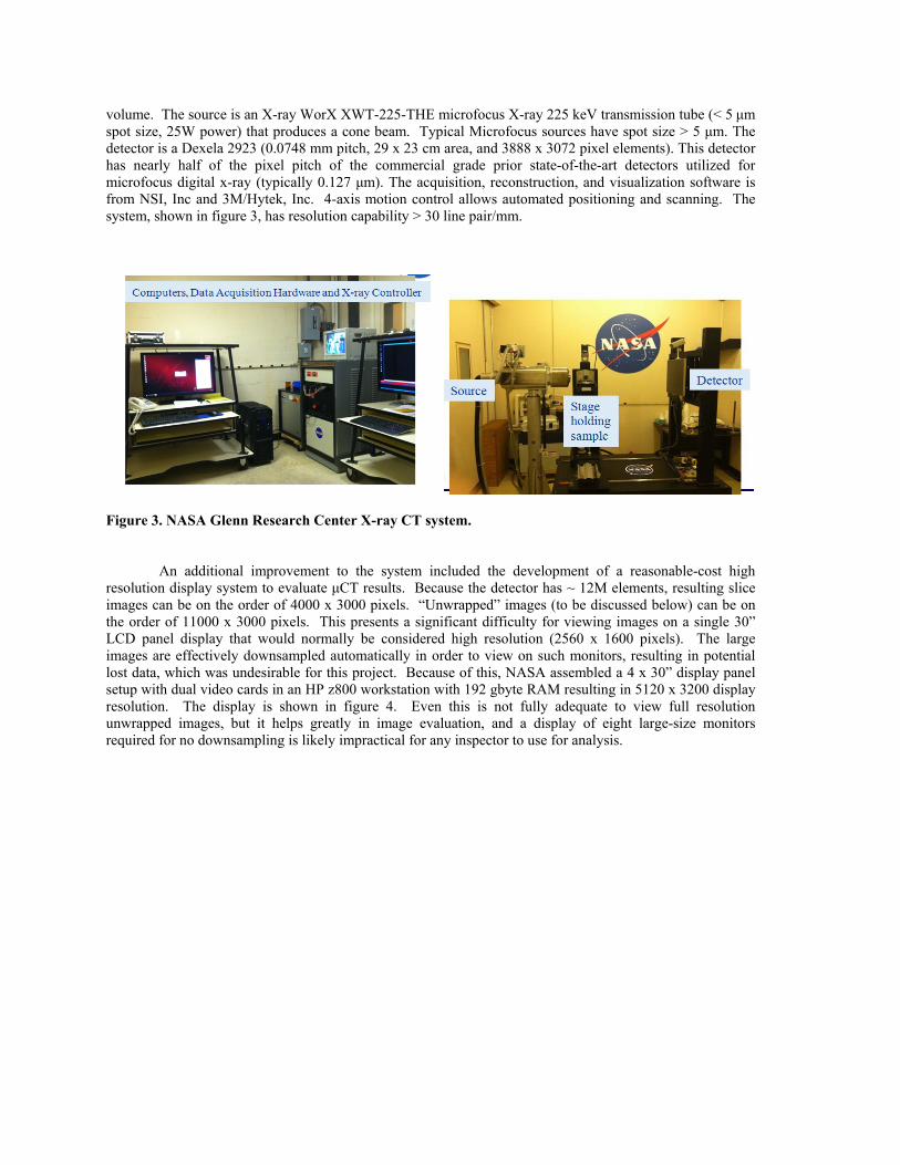
volume. The source is an X-ray WorX XWT-225-THE microfocus X-ray 225 keV transmission tube (< 5 μm spot size, 25W power) that produces a cone beam. Typical Microfocus sources have spot size > 5 μm. The detector is a Dexela 2923 (0.0748 mm pitch, 29 x 23 cm area, and 3888 x 3072 pixel elements). This detector has nearly half of the pixel pitch of the commercial grade prior state-of-the-art detectors utilized for microfocus digital x-ray (typically 0.127 μm). The acquisition, reconstruction, and visualization software is from NSI, Inc and 3M/Hytek, Inc. 4-axis motion control allows automated positioning and scanning. The system, shown in figure 3, has resolution capability > 30 line pair/mm.

Figure 3. NASA Glenn Research Center X-ray CT system.

An additional improvement to the system included the development of a reasonable-cost high

resolution display system to evaluate μCT results. Because the detector has ~ 12M elements, resulting slice images can be on the order of 4000 x 3000 pixels. “Unwrapped” images (to be discussed below) can be on the order of 11000 x 3000 pixels. This presents a significant difficulty for viewing images on a single 30” LCD panel display that would normally be considered high resolution (2560 x 1600 pixels). The large images are effectively downsampled automatically in order to view on such monitors, resulting in potential lost data, which was undesirable for this project. Because of this, NASA assembled a 4 x 30” display panel setup with dual video cards in an HP z800 workstation with 192 gbyte RAM resulting in 5120 x 3200 display resolution. The display is shown in figure 4. Even this is not fully adequate to view full resolution unwrapped images, but it helps greatly in image evaluation, and a display of eight large-size monitors required for no downsampling is likely impractical for any inspector to use for analysis.

Figure 4. Four 30” monitor visualization setup showing one unwrapped CT reslices for the heater head spanning the four monitors. (Upper left hand corner shows thumbnail image of a CT cross-sectional slice which when “unwrapped” results in the CT reslices shown spanning the four monitors.) UNWRAPPER/RESLICER SOFTWARE

CT data visualization in the heater head presents an immense challenge from the human factors standpoint. This is because ultra-thin-wall metallic cylinders are extremely difficult to analyze for flaws from top-view cross-sectional CT slices and volume renderings. Top view slice images for the heater head are extremely difficult to evaluate for flaw indications because the wall is so thin, and extensive zooming and panning is required when viewing each slice. Additionally, the inner wall is ill-defined at the low voltage settings utilized (the lowest voltage possible was utilized while still achieving acceptable photon count at the detector in order to obtain optimal contrast for flaw detection (see figure 5)). (Higher voltage and lower current settings with total power near the tube power rating of 25W allows resolution of the inner wall at the expense of flaw contrast.) With thousands of slices, analysis using top view slices is totally impractical. Volume rendering grayscale, texture and contrast expansion schemes that highlight the flaws of interest also tend to highlight graphic anomalies in the cartoon-like renderings. Thus, it is difficult to separate flaw from graphic anomalies in the volume renderings. Computerized automatic flaw recognition was developed but proved only mildly successful due to widely varying flaw indication gray scale and also very slow for the large data sets.

In general for cylindrical CT data flaw detection, it can be advantageous to unwrap and reslice the 360o data so as to view 2-d “sheets” from the exterior to interior of the cylinder separated by the voxel dimension. For this work, it became essential to perform this process because flaws were so difficult to detect from both top view slices and volume renderings. NASA GRC developed dedicated cylindrical CT data unwrapper/reslicer software (CT-CURS) [4] for just this purpose. Accurate lateral dimensional analysis of flaw dimensions is only possible on the unwrapped sheets. Additionally, unwrapping allows the viewing of a reasonable number of large CT slices from exterior to interior of a cylindrical object. Further, there is no data set size restriction when using this software which is critical for the up-to-40 gbyte data sets for the heater head. To effectively unwrap and reslice the CT data, the cross-sectional CT slices must be histogram-matched and precisely aligned. Software to perform sub-voxel resolution alignment is included as a pre-processing step in CT-CURS. Each unwrapped reslice is contrast expanded between its minimum and maximum value, and flaws tend to “jump out” at the inspector on the reslices. Additionally, many image processing and quantitative analysis tools are available in the software to enhance flaw detectability and make flaw measurements. Perhaps the most significant of these is the ability to point and click on flaws on the unwrapped reslices. This results in the automated recall of the proper top view slice, and draws a line from

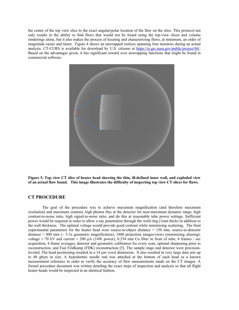
the center of the top view slice to the exact angular/polar location of the flaw on the slice. This protocol not only results in the ability to find flaws that would not be found using the top-view slices and volume renderings alone, but it also makes the process of locating and characterizing flaws, at minimum, an order of magnitude easier and faster. Figure 4 shows an unwrapped reslices spanning four monitors during an actual analysis. CT-CURS is available for download by U.S. citizens at https://sr.grc.nasa.gov/public/project/86/. Based on the advantages given, it has significant reward over unwrapping functions that might be found in commercial software.

Figure 5. Top view CT slice of heater head showing the thin, ill-defined inner wall, and exploded view of an actual flaw found. This image illustrates the difficulty of inspecting top view CT slices for flaws. CT PROCEDURE The goal of the procedure was to achieve maximum magnification (and therefore maximum resolution) and maximum contrast, high photon flux at the detector for near-maximum dynamic range, high contrast-to-noise ratio, high signal-to-noise ratio, and do this at reasonable tube power settings. Sufficient power would be required in order to allow x-ray penetration through the weld ring (1mm thick) in addition to the wall thickness. The optimal voltage would provide good contrast while minimizing scattering. The final experimental parameters for the heater head were source-to-object distance = 150 mm, source-to-detector distance = 800 mm (~ 5.3x geometric magnification), 1800 projection images/views (minimizing aliasing), voltage = 70 kV and current = 200 μA (14W power), 0.254 mm Cu filter in front of tube, 4 frames / sec acquisition, 4 frame averages, detector and geometric calibration for every scan, optimal sharpening prior to reconstruction, and Fast Feldkamp (FDK) reconstruction [5]. The sample stage and detector were precision-leveled. The head positioning resulted in a 14 μm voxel dimension. It also resulted in very large data sets up to 40 gbyte in size. A hypodermic needle end was attached at the bottom of each head as a known measurement reference in order to verify the accuracy of flaw measurements made on the CT images. A formal procedure document was written detailing the exact steps of inspection and analysis so that all flight heater heads would be inspected in an identical fashion.

PROBABILITY OF DETECTION

A spare heater head of identical structure to actual heater heads had four artificial flaw patterns machined into its wall using a micro electrical discharge machining (micro-EDM) procedure. Hole and slit patterns were machined into both the thin and taper wall regions using the micro-EDM procedure with one hole pattern and one slit pattern in each region to create a calibration standard. The specification was for holes ranging in diameter from 40 – 120 μm and ranging in depth from 60 μm to – full wall penetration. The slits were to range in depth from 60 – 80 μm, in width from 20 – 70 μm , and in length from 40 - 1200 μm. Approximately 120 and 40 flaws were machined into the thin wall and taper wall (at location ~ 2.5x thickness of thin wall), respectively. The bottom of the flaws was reasonably flat. The machined flaws’ depths were measured using a combination of electrode encoder position as provided by the vendor and optical microscopy at NASA (and from CT measurements in a limited number of cases). The vendor specified a 1 – 2 μm depth accuracy while NASA expected a 5 – 10% depth measurement error in the optical measurement. Lateral dimensions were measured using scanning electron microscopy (SEM) with an estimate of 5 – 10% accuracy. CT depth measurement error was estimated overall between 10 – 30% (discussed below).

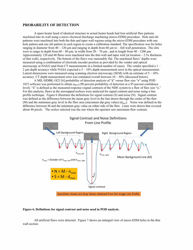
A MIL-HDBK-1823 [6] probability of detection analysis of “â” versus flaw size “a” using POD 1823 software was performed to obtain a90/95 (90 percent probability of detection at a 95 percent confidence level). “â” is defined as the measured response (signal contrast) of the NDE system to a flaw of flaw size “a.” For this analysis, flaws in the unwrapped reslices were analyzed for signal contrast and noise using a line profile technique. Figure 6 illustrates the definitions for signal contrast (S) and noise (N). Signal contrast was defined as the difference between the mean gray level in the line drawn through the center of the flaw (M) and the minimum gray level in the flaw area (maximum dip gray value) (dmax). Noise was defined as the difference between M and the minimum gray value on either side of the flaw. Lines were drawn that covered about 40 pixels. The reslice selected was the one where the operator saw maximum flaw contrast.

Signal Contrast and Noise DefinitionsFrom Line Profile

Signal contrast

nmax, left

nmax = Greater of nmax, left and nmax, right

nmax, right

Mean Background Line (M)

Quantities shown are Gray Values obtained from the Image Line Profile

Left Background Region Right  Background Region

• N = M ‐ nmax

• S = M ‐ dmax

dmax

Figure 6. Definitions for signal contrast and noise used in POD analysis.

All artificial flaws were detected. Figure 7 shows an enlarged view of micro-EDM holes in the thin wall section.

______ 1 mm Figure 7. Micro-EDM hole pattern (unwrapped-resliced CT view) in thin wall section near outer diameter surface. POD analysis required plotting signal contrast versus volume of the flaw since both depth and lateral dimensions will play a role in detectability. The micro-EDM holes and slits were modeled as cylinders and rectangular boxes, respectively. For the POD analysis, a model is selected that provides the most linear relationship between signal contrast and volume. For this data, a linear (Y axis) – log (X-axis) model provided the most linear relationship. Some data points were identified as outliers for the purpose of the analysis. Figure 8 shows signal contrast versus log (flaw volume) for the micro-EDM holes in the thin wall region.

Figure 8. Signal Contrast vs. Log (Flaw Volume) for the micro-EDM holes in the thin wall region. The analysis also requires a decision threshold to be selected which is normally the lowest contrast value observed in the data set. The decision threshold is defined as the value of â above which the signal is interpreted as a hit, and below which the signal is interpreted as a miss. The decision threshold is the â value associated with 50% POD and is always greater than the inspection threshold (the lowest possible signal contrast that might be interpreted as a hit) [6]. Figure 9 shows Probability of Detection vs. Volume for the micro-EDM holes in the thin wall region. The volumes for 50% POD, 90% POD, and 90% with 95% confidence bounds POD are shown.

y = 149.36x ‐ 732.37R² = 0.9121

‐50

0

50

100

150

200

250

300

0 2 4 6 8

Contrast (gray value)

Log (Volume, um^3)

C (gray value): Holes in Thin Wall

Linear (C (gray value): Holes in Thin Wall)

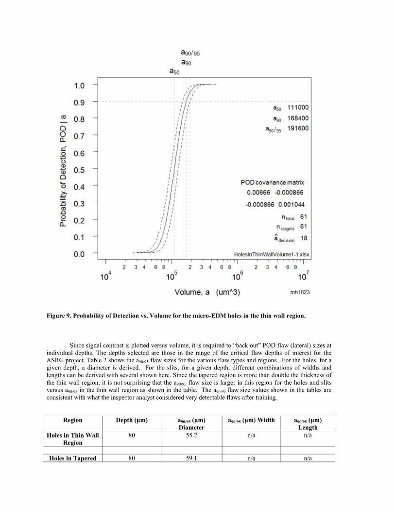
Figure 9. Probability of Detection vs. Volume for the micro-EDM holes in the thin wall region.

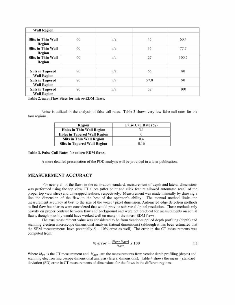
Since signal contrast is plotted versus volume, it is required to “back out” POD flaw (lateral) sizes at individual depths. The depths selected are those in the range of the critical flaw depths of interest for the ASRG project. Table 2 shows the a90/95 flaw sizes for the various flaw types and regions. For the holes, for a given depth, a diameter is derived. For the slits, for a given depth, different combinations of widths and lengths can be derived with several shown here. Since the tapered region is more than double the thickness of the thin wall region, it is not surprising that the a90/95 flaw size is larger in this region for the holes and slits versus a90/95 in the thin wall region as shown in the table. The a90/95 flaw size values shown in the tables are consistent with what the inspector analyst considered very detectable flaws after training.

Region Depth (μm) a90/95 (μm) Diameter

a90/95 (μm) Width a90/95 (μm) Length

Holes in Thin Wall Region

80 55.2 n/a n/a

Holes in Tapered 80 59.1 n/a n/a

Wall Region

Slits in Thin Wall Region

60 n/a 45 60.4

Slits in Thin Wall Region

60 n/a 35 77.7

Slits in Thin Wall Region

60 n/a 27 100.7

Slits in Tapered

Wall Region 80 n/a 65 80

Slits in Tapered Wall Region

80 n/a 57.8 90

Slits in Tapered Wall Region

80 n/a 52 100

Table 2. a90/95 Flaw Sizes for micro-EDM flaws. Noise is utilized in the analysis of false call rates. Table 3 shows very low false call rates for the four regions.

Region False Call Rate (%)

Holes in Thin Wall Region 3.1 Holes in Tapered Wall Region 0

Slits in Thin Wall Region 0.4 Slits in Tapered Wall Region 0.16

Table 3. False Call Rates for micro-EDM flaws. A more detailed presentation of the POD analysis will be provided in a later publication. MEASUREMENT ACCURACY For nearly all of the flaws in the calibration standard, measurement of depth and lateral dimensions was performed using the top view CT slices (after point and click feature allowed automated recall of the proper top view slice) and unwrapped reslices, respectively. Measurement was made manually by drawing a line the dimension of the flaw to the best of the operator’s ability. The manual method limits the measurement accuracy at best to the size of the voxel / pixel dimension. Automated edge detection methods to find flaw boundaries were considered that would provide sub-voxel / pixel resolution. Those methods rely heavily on proper contrast between flaw and background and were not practical for measurements on actual flaws, though possibly would have worked well on many of the micro-EDM flaws.

The true measurement value was considered to be from vendor-supplied depth profiling (depth) and scanning electron microscope dimensional analysis (lateral dimensions) (although it has been estimated that the SEM measurements have potentially 5 – 10% error as well). The error in the CT measurements was computed from:

%| |

100 (1)

Where is the CT measurement and are the measurements from vendor depth profiling (depth) and scanning electron microscope dimensional analysis (lateral dimensions). Table 4 shows the mean + standard deviation (SD) error in CT measurements of dimensions for the flaws in the different regions.

Region / Number of Measurements

Mean + SD Error in Depth

Measurement (%)

Mean + SD Error in Diameter

Measurement (%)

Mean + SD Error in Length

Measurement (%)

Mean + SD Error in Width Measurement

(%) Holes in Thin Wall

Region / 66 10 + 9 33 + 22 n/a n/a

Holes in Tapered Wall Region / 21

10 + 9 20 + 16 n/a n/a

Slits in Thin Wall

Region / 62 13 + 13

n/a 14 + 19 22 + 22

Slits in Tapered Wall Region / 17

12 + 7

n/a 13 + 10

20 + 12

Table 4. Percent Mean + Standard Deviation (SD) Error in CT measurements of Dimensions Using Manual Measurement by CT Operator. Computations are rounded to nearest whole number. Note that the mean % error in depth (critical flaw) dimension was at or near 10% with ~ 10% standard deviation. Lateral measurement % error was between 10% and 35% with standard deviation % error ranging from 10% to 22%. These are large standard deviations that represent a significant spread in the CT measurement accuracy. The spread is illustrated in figure 10 which shows the % error in CT depth measurement vs. hole number for the holes in the thin wall region. The trend line in figure 10 hovers near the observed mean % error (10%).

Figure 10. % Error in CT depth measurement vs. Hole number. RESULTS ON ACTUAL HEATER HEADS

Figure 11 shows CT results from several of the flight heater heads. The flaws found in the heads were determined to be primarily oxide inclusions of various compositions (see section entitled “CORRELATION OF CT RESULTS WITH OPTICAL AND SEM RESULTS”) as a result of the casting process. (By viewing these flaws it is apparent that a threshold-based automatic flaw recognition scheme would not be practical due to the differing gray scales of the flaws against an image that itself contains gray scale variation (noise).)

0

5

10

15

20

25

30

35

40

45

50

1 5 9 13 17 21 25 29 33 37 41 45 49 53 57 61 65 69 73 77 81 85 89 93 97

% Error

Hole Number

CT Depth Error (%) vs. Hole Number

Trend line

.

5.0 mm Oxide0.354 mm Oxide

Unwrapped ResliceView (Length) Top View (Depth)

0.54 mm Oxide 0.280 mm Oxide

0.40 mm Oxide 0.351 mm Oxide

zr

Figure 11. CT results showing lateral and depth views of three flaws in actual heater head sample. Lateral size and depth are provided from measurements in the unwrapped reslices and top views, respectively, where ‘z’ is the axial direction upward and ‘r’ is radial direction. CORRELATION OF CT RESULTS WITH OPTICAL AND SEM RESULTS For the flight heater heads that failed CT inspection and could be sectioned, excellent correlation between lateral flaw indications from the CT unwrap reslices and optical and scanning electron microscope (SEM) results was consistently observed (as seen in figure 12).

16

CT Unwrap View / Reslice

SEM

Optical

Appearance of the Major Flaw Using Different Imaging Techniques

Both the optical and SEM images suggest that the defect is not porosity but rather a solid phase of some type.

Figure 12. Correlation between CT, Optical, and SEM results. BRAZE JOINT EVALUATION

The porosity fraction of the braze joint was evaluated per American Welding Society Specification for Furnace Brazing, AWS C3.6M / C3.6: 2008 Section 6.5.2 [3] using the unwrapped reslice where the pores became most focused. The braze joint is about 0.2 mm thick and the CT does an excellent job of characterizing pore fraction, size, and location as shown in figure 9 for a development heater head. The CT-CURS software has a binary threshold image processing operation to binarize the images, followed by an automated areal fraction quantitative image analysis to calculate porosity fraction. In the example shown in figure 13, even though there is significant porosity in one area of the braze joint, the % porosity in the entire braze joint is only 2.2%. However, the near inter-connectedness of porosity of several regions would likely have resulted in failure to meet the AWS specification (the width of the largest void or unbounded area as measured parallel to the joint width shall not exceed 60% of the total joint width and / or any such void that is wider than 40% of the width of the joint shall extend no closer to either edge of the joint than 20% of the joint width).

Sample CT Results

Unwrapped View –One Reslice

2.2% Porosity

Binary thresholding of entire braze joint area, coloring porosity red and all other material colored black

Figure 13. CT volume rendering, unwrapped reslices view, and magnified view of braze joint porosity. Braze joint region of image is binarized using threshold method and areal fraction of porosity automatically calculated in CT-CURS. The % porosity in the entire braze joint is 2.2%. USE OF CT DATA FOR LIFE MODELING

The ASRG program later required the inspection analyst to measure as accurately as possible flaw depth, flaw length, angle from vertical, X and Y location, and distance from open end. The CT results were used as inputs to analytical modeling which determines whether a flaw(s) in a heater head will create a leak path within four service lifes. If the model predicted such a leak path, the heater head could not be placed into flight service. The model was fracture mechanics-based and required calculation of a “damage index” that was dependent on the total number of expected loading events, the number of expected cycles for each event (such as from cyclical vibration loads during rocket launching), applied stress, flaw geometry, and component geometry). If the damage index > 1.0, leaking is expected with four service lifes. If the damage index << 1.0, leaking is not expected with four service lifes. This modeling effort requires accurate flaw morphology information which can only be obtained practically using high resolution Microfocus CT.

CONCLUSIONS A high resolution micro-computed tomography (μCT) system complemented by specialized

hardware and software tools were used to provide quantitative characterization for a tapered ultra-thin wall space component at NASA. The CT data served two purposes: first to assess whether an acceptable flaw condition based on requirements existed and second to provide comprehensive flaw measurements for life modeling. No other characterization options are practical or possible for such a complex-shaped component requiring high fidelity measurements. POD characterization and measurement accuracy of the method were assessed. The CT method should be considered essential for characterization of high-performance reasonably-sized components in critical aerospace applications.

REFERENCES

1. “NASA Space Technology Roadmaps and Priorities: Restoring NASA’s Technological Edge and Paving the Way for a New Era in Space,” National Research Council, National Academy Press, Washington, D.C., 2012.

2. Elmo, T., “Advanced Stirling Radioisotope Generator,” Loc Publishing, 2012. 3. “Specification for Furnace Brazing,“ AWS specification C3.6M/C3.6:2008, Section 6.5.2, American

Welding Society, 2008. 4. Roth, D.J., Burke, E.R., Rauser, R.W., and Martin, R.E., “A Novel Automated Method For Analyzing

Cylindrical Computed Tomography Data,” Extended Abstract Paper Proceedings at Fall 2011 ASNT conference. Palm Springs Convention Center, Palm Springs, California. October 24 – 28. Pp. 139 – 145.

5. Feldkamp, L.A., Davis, L.C., and Kress, J.W., “Practical cone-beam algorithm,” J. Opt. Soc. Amer. A6 (1984), 612 – 619.

6. MIL-HDBK-1823, DEPARTMENT OF DEFENSE HANDBOOK: NONDESTRUCTIVE EVALUATION (NDE) SYSTEM, RELIABILITY ASSESSMENT (30 APR 1999).