the cost of immediacy for corporate bonds · effects, months before the actual index revision date....
TRANSCRIPT
[17:21 17/12/2018 RFS-OP-REVF180082.tex] Page: 1 1–41
The Cost of Immediacy for Corporate Bonds
Jens Dick-NielsenCopenhagen Business School
Marco RossiTexas A&M University
Liquidity provision for corporate bonds has become significantly more expensive after the2008 crisis. Using index exclusions as a natural experiment during which uninformed indextrackers request immediacy, we find that the cost of immediacy has more than doubled.In addition, the supply of immediacy has become more elastic with respect to its price.Consistent with a stringent regulatory environment incentivizing smaller dealer inventories,we also find that dealers revert deviations from their target inventory more quickly afterthe crisis. Finally, we investigate the pricing impact of information, changes in ownershipstructure, and differences between bank and nonbank dealers. (JEL C23, G12)
Received February 22, 2017; editorial decision May 29, 2018 by Editor Itay Goldstein.Authors have furnished an Internet Appendix, which is available on the Oxford UniversityPress Web site next to the link to the final published paper online.
Liquidity entails transacting at a fair price and on short notice. Low bid-askspreads may indicate transactions take place near a fair price, but they tell littleabout the speed of execution. Unlike brokers who simply match customers,dealers provide immediacy by using their inventories.1 Since the onset of the2008 crisis, aggregate corporate bond inventories have shrunk by more than50% (Figure 1A), while bonds outstanding have almost doubled.2 Shrinking
We are grateful to Itay Goldstein (the editor) and two anonymous referees for their helpful feedback andsuggestions. We also thank Jennie Bai, Jack Bao, Darrell Duffie, Peter Feldhütter, Thierry Foucault, JeanHelwege, Charles Himmelberg, Soeren Hvidkjaer, David Krein, David Lando, Mads Stenbo Nielsen, LasseHeje Pedersen, Christophe Perignon, Jonathan Sokobin, Chester Spatt, Ilya Strebulaev, Erik Thiessen, KumarVenkataraman, and Avi Wohl and participants of the Fixed Income Conference 2012, MFA conference 2012,FINRA/Columbia conference 2015, 2016 4Nations cup, Corporate bond workshop 2016, Financial Econometricsand Empirical Asset Pricing Conference 2016, MIT GCFP conference 2016, Notre Dame conference on financialregulation 2016, 14th Paris December Finance Meeting 2016, AFA conference 2017, Macro Financial ModellingConference 2018, and SEC, FCA, Danish CFA, CBS, SMU, Texas A&M, Notre Dame, Heriot-Watt University,and Helsinki Aalto seminars for their helpful comments. Special thanks goes to Jonathan Sokobin (FINRA) forproviding the transaction data and Charles Himmelberg (Goldman Sachs) for providing the aggregate corporatebond inventory data. This paper won second prize in the 2012 SPIVA awards and first place in the 2016 4Nationscup. Jens Dick-Nielsen is a research fellow at the Danish Finance Institute and gratefully acknowledges supportfrom the FRIC Center for Financial Frictions [DNRF102]. Supplementary data can be found on The Review ofFinancial Studies Web site. Send correspondence to Jens Dick-Nielsen, Copenhagen Business School, SolbjergPlads 3, 2000 Frederiksberg, Denmark. E-mail: [email protected].
1 See Garman (1976), Stoll (1978), Amihud and Mendelson (1980), and Ho and Stoll (1981).
2 See, for example, the 2017 SIFMA Fact Book.
© The Author(s) 2018. Published by Oxford University Press on behalf of The Society for Financial Studies.All rights reserved. For permissions, please e-mail: [email protected]:10.1093/rfs/hhy080 Advance Access publication July 24, 2018
Dow
nloaded from https://academ
ic.oup.com/rfs/article-abstract/32/1/1/5058062 by guest on 15 O
ctober 2019

[17:21 17/12/2018 RFS-OP-REVF180082.tex] Page: 2 1–41
The Review of Financial Studies / v 32 n 1 2019
inventories amid a growing bond market suggest that providing immediacy hasbecome more difficult, but because we rarely observe expensive trades requiringimmediacy, focusing on realized transactions understates liquidity costs.3 Anunconditional analysis of transaction costs is particulary problematic if tradersanticipate or experience significant changes in market structure and regulatoryframework during the sample period. In the spirit of the Lucas (1976) critique,regulations increasing the cost of immediacy may induce market participantsto optimally, albeit reluctantly, adjust their trading behavior.
The main contribution of this study is to quantify the cost of immediacy forcorporate bonds in a trading environment that circumvents the Lucas (1976)critique. We identify trades in which the motive to obtain immediacy is sostrong that liquidity seekers do not orchestrate alternative trading arrangements.Furthermore, these trades reveal no information about the fundamental valueof the assets traded. Specifically, we compute liquidity costs around exclusionsfrom the Barclay Capital investment-grade corporate bond index. In this naturalexperiment, index trackers (the sellers) request immediacy from dealers (thebuyers) in order to minimize their tracking error. Moreover, mechanical indexrules, not fundamentals, dictate the decision to trade, thus ensuring that thedealer’s pricing reflects the cost of providing immediacy, rather than the adverseselection problem of dealing with informed traders (Easley and O’Hara 1987).
We show that the price of immediacy has more than doubled since before the2008 crisis. Our empirical analysis also shows that the price elasticity of thesupply of immediacy has increased significantly after the crisis. This increasein elasticity is indicative of higher market-making costs, which translates intohigher average transaction costs, thus providing support for standard theoriesof market maker inventories. For safe bonds, which are quickly turned overagain by dealers, the cost of immediacy has approximately doubled, whereasfor more risky bonds, the cost has more than tripled.
We infer the cost of immediacy by computing a dealer-specific abnormalbond return. We do this by defining an intertemporal bid-ask spread, which isbased on the percentage difference between the post-exclusion ask price andthe pre-exclusion bid price. This measure captures the essence of the dealer’srole, who uses her inventory to absorb the selling pressure generated by theindex trackers unloading their positions, and then resells the bonds to restorethe desired level of inventory. These dealer returns indicate that the cost ofproviding immediacy has increased in the post-crisis, low-inventory regime.
Before measuring transaction costs around index exclusions, we verifythat these exclusions are indeed events during which index trackers requestimmediacy. Our analysis reveals that the traded volume of bonds exiting theindex peaks during the day of the exclusion, and it is at least 4 to 5 times higherthan that in the surrounding weeks. The peak in trading volume is consistent
3 For instance, Trebbi and Xiao (2017), Adrian et al. (2015), and Bessembinder et al. (2018) find that realizedtrading costs have improved.
2
Dow
nloaded from https://academ
ic.oup.com/rfs/article-abstract/32/1/1/5058062 by guest on 15 O
ctober 2019

[17:21 17/12/2018 RFS-OP-REVF180082.tex] Page: 3 1–41
The Cost of Immediacy for Corporate Bonds
Primary dealer inventory
Corp
. sec. in
vento
ry (
US
D b
n)
050
100
150
200
250
300
Jan03 Jan07 Jan11 Jan15
Corporate securities
Corporate bonds
Corp
. bond inve
nto
ry (
US
D b
n)
10
15
20
25
30
Market illiquidity factor
Mark
et ill
iqudity facto
r
−1
01
23
45
Jan03 Jan07 Jan11 Jan15
A
B
Figure 1Corporate bond market statisticsPanel A shows the primary dealer inventories in corporate securities (investment grade more than 1 year inmaturity) and in corporate bonds. The first series can be retrieved from the New York Fed statistics on primarydealer holdings. The graph on corporate bonds can be retrieved from the same place after March 2003. Thenumbers prior to that date have been computed by Goldman Sachs using yearly SEC filings from the primarydealers. Panel B shows the market liquidity measure from Dick-Nielsen, Feldhutter, and Lando (2012). Themeasure can be downloaded from peterfeldhutter.com
with index trackers attempting to minimize their tracking errors by trading closeto the index exclusion date.4 Back-of-the-envelope calculations indeed showthat reluctance to trade away from the exclusion date results in a hidden costof indexing5 for final investors of approximately 34 bps annually.
Having established the existence of a demand for immediacy, we verify thatdealers absorb the resultant selling pressure and thus provide such immediacy.Dividing the sample into three subperiods shows that dealer behavior has
4 Blume and Edelen (2004) show that stock index trackers display a similar behavior.
5 See also Chen, Noronha, and Singal (2006), Petajisto (2011), and Pedersen (2018) about this cost.
3
Dow
nloaded from https://academ
ic.oup.com/rfs/article-abstract/32/1/1/5058062 by guest on 15 O
ctober 2019

[17:21 17/12/2018 RFS-OP-REVF180082.tex] Page: 4 1–41
The Review of Financial Studies / v 32 n 1 2019
changed after the crisis. Our analysis of the cumulative change in inventoriesdemonstrates that dealers’ willingness to hold the bonds in their inventorieshas declined in the post-crisis, low-inventory regime. While before (and evenduring) the crisis dealers kept a large share of bonds downgraded out of the indexfor at least 100 days, after the crisis the inventories return to near pre-exclusionlevels within approximately 20 trading days. More formally, we estimate dealer-specific inventory mean reversion parameters following Madhavan and Smidt(1993) and find that after the 2008 crisis dealers are less willing to toleratedeviations from their desired level of inventory. The estimated inventory half-life significantly decreases from before to during and from during to after thecrisis. These findings suggest an increase in inventory costs of market makers.
We conclude our empirical analysis by exploring several potential channelsleading to a higher price of immediacy. First, using institutional bond holdings,we document an increased role of mutual funds in the corporate bond space.We find that both insurance companies and mutual funds are net sellers aroundexclusions, a change of behavior for mutual funds that used to trade in the samedirection as dealers before the crisis. We control for these demand shifts in ourmultivariate analysis and find that, while important, these shifts do not affectthe conclusion that dealers’ supply elasticity is higher after the crisis. Second,we control for contemporaneous new information potentially affecting bondprices and find that it does not affect earlier conclusions. Third, we test a setof predictions based on search models. The results of our test suggest that theincrease in the cost of immediacy is consistent with an increase in inventoryholding costs and not driven by an increase in dealer market power.
In addition to contributing to the literature on corporate bond liquidity,this paper occupies a natural place in the literature connecting regulationsto financial market efficiency. The debate on the repercussions of the Dodd-Frank act on the financial system offers positions that view the regulatorychanges as potentially harmful (Duffie 2012) as well as beneficial (Richardson2012). Our study cautions against drawing conclusions about liquidity based onrealized aggregate transaction costs. Liquidity measures, such as the one shownin Figure 1B, are the outcome of market participants’ optimization problems,and a large-scale policy change alters the optimal behavior of investors anddealers. An analogy would be new rules that significantly increased the costof air travel would induce more travelers to use the bus instead. Discouragingair travel might well lower the average realized cost of transportation (takingthe bus is cheaper), but average utility would decline because of the loss ofimmediacy. Traveling from Los Angeles to New York in 3 days by bus is notthe same as completing the trip in 5 hours by plane.
By focusing on a homogenous, information-free event in which agents donot arrange alternative trading strategies before and after the suggested policychange, our analysis is able to uncover the potential adverse effect that thenew regulatory, low-inventory regime has had on corporate bond liquidity.Separating dealers into banks and nonbanks, we show that the post-crisis change
4
Dow
nloaded from https://academ
ic.oup.com/rfs/article-abstract/32/1/1/5058062 by guest on 15 O
ctober 2019

[17:21 17/12/2018 RFS-OP-REVF180082.tex] Page: 5 1–41
The Cost of Immediacy for Corporate Bonds
in dealer behavior is most pronounced for banks. This finding is consistentwith banks unwinding proprietary trading in response to anticipated tighterregulation, specifically the Volcker rule. Our paper thus complements otherrecent papers in this area by documenting an anticipation effect on the cost ofimmediacy closely linked to dealers’ inventory costs. Using a more recentsample that covers the implementation of the Volcker rule, Bao, O’Hara,and Zhou (2018) confirm its adverse impact on liquidity provision. Similarly,Bessembinder et al. (2018) provide evidence that dealers are less willing tocommit overnight capital after the crisis.
Our paper also contributes to the literature on index revisions and tradingaround predictable events (see, e.g., Admanti and Pfleiderer, 1991).6 Bondindex revisions have been recently studied by Newman and Rierson (2004) andChen et al. (2014), but these authors focus on special one-time announcementeffects, months before the actual index revision date. Newman and Rierson(2004) look at a large and unique issuance event for European telecomcompanies. Chen et al. (2014) look at the effect of a unique rating rule changefor the Lehman index. Unlike these studies, our paper looks at the trading veryclose to the actual index revision dates.
1. Corporate Bond Index Tracking
We consider exclusions from the Barclay Capital corporate bond Index, whichwas previously known as the Lehman corporate bond Index and is currentlycalled the Bloomberg-Barclay corporate bond Index. These exclusions providean ideal natural experiment for studying the cost of immediacy over time. Eachmonth corporate bond index trackers demand immediacy from dealers whenthey seek to sell bonds exiting the index.
That the rules for bonds entering or exiting the index are both transparentand mechanical makes the monthly exclusion events information-free andhomogeneous over time. As of July 2005, the index contains all U.S. corporatebond issues with an investment-grade rating by at least two of the three majorrating agencies (Standard and Poor’s, Moody’s, and Fitch). Furthermore, theissuance size must be at least $250 million and time to maturity must be morethan 1 year.7 Bonds exit the index for three main reasons: time to maturitybecomes less than 1 year; issuers call their bonds; their median rating goesfrom investment grade to speculative grade, so if for instance only two ratingsare available, the lower and more conservative rating is used. Bonds enter theindex for two main reasons: if they are newly issued and index eligible or if the
6 See, for example, Chen, Noronha, and Singal (2004) for studies on equity index revisions and Lou, Yan, andZhang (2013) for anticipated trading in the Treasury market.
7 Index eligibility requires more qualitative rules. See the index rules at https://ecommerce.barcap.com/indices/index.dxml
5
Dow
nloaded from https://academ
ic.oup.com/rfs/article-abstract/32/1/1/5058062 by guest on 15 O
ctober 2019

[17:21 17/12/2018 RFS-OP-REVF180082.tex] Page: 6 1–41
The Review of Financial Studies / v 32 n 1 2019
Table 1Barclay Capital Corporate Bond Index exclusion statistics
A. Index exclusions
Reason N Market value ($1,000) OA duration Coupon
Maturity<1 3,102 645,374 0.92 5.7Called 392 461,354 0.52 7.1Downgrade 1,078 484,269 5.1 6.8Other 2,119 358,501 6.0 6.5
B. Bond presence in TRACE
Reason Total excluded In TRACE Traded Soldat exclusion at exclusion
Maturity<1 3,102 2,732 2,532 2,452Downgrade 1,078 893 804 792
The statistics are accumulated from July 2002 to November 2013 for the Barclay Corporate Bond Index (formerlyLehman). Panel A shows characteristics for the excluded bonds. Market value represented in $1,000 US is theaverage market value at the time of the index revision. The table shows four reasons for being excluded. Thematurity of the bonds can fall less than 1 year during the month. The bond can be called. The bond can bedowngraded from investment grade to speculative grade during the month. Additionally, the bond can be excludedfor various other reasons. Most of these exclusions are due to revisions of the general index rules, mainly thatthe size requirement has been increased twice over the period. In all cases, the bonds are excluded at the endof the month (last trading day). Panel B shows the number of excluded bonds with transactions in TRACE, thenumber of bonds traded at exclusion (event day -2 to 0), and the number of bonds sold (bought) by customers(dealers) at exclusion.
rating goes from speculative grade to investment grade.8 These rules result inan index that covers a large fraction of the market. The index is rebalanced oncea month on the last trading day of the month at 3:00 pm EST and all bonds thatare no longer index eligible are excluded at this point in time. We note that theactual downgrade date of a bond takes place before the bond is excluded fromthe index, so in principle it represents a separate event from exclusion itself.(We explore actual downgrades in Section 5.3.)
Our bond sample consists of all bonds exiting the index between July 2002and November 2013. Exclusions are fairly equally scattered over time as seenin Figure 2. Table 1, panel A, gives characteristics of the excluded bonds. Alarge number of bonds have been excluded from the index for other reasons.These exclusions are mainly due to an increase in the lower size limit for indexeligibility, which is why the average issuance size of these bonds is far less thanfor the rest of the sample.
The objective of index trackers is to minimize tracking error between thereturn on their portfolio and that of the index. Blume and Edelen (2004) showthat index trackers following the S&P 500 index are transacting on the exact daythat the index is rebalanced, even though they sacrifice potential profit by doingso (Beneish and Whaley 1996). Low tracking error is a signal to investors thatthe index tracker is in fact committed to tracking the index and thus resolvesan agency problem.
8 We do not report results for index inclusions, because there is little price pressure at inclusion events. Indextrackers sample the index, so they can select which bonds to buy and thus have a selection of maybe 10–30 bondsbut only need to buy 3–10 bonds. This freedom in selection alleviates most of the price pressure.
6
Dow
nloaded from https://academ
ic.oup.com/rfs/article-abstract/32/1/1/5058062 by guest on 15 O
ctober 2019

[17:21 17/12/2018 RFS-OP-REVF180082.tex] Page: 7 1–41
The Cost of Immediacy for Corporate Bonds
Maturity < 1 year
01
02
03
04
05
06
07
0
Jan03 Jan05 Jan07 Jan09 Jan11 Jan13
Number of bonds
Number of firms
Rating less than investment grade
01
02
030
40
50
60
70
Jan03 Jan05 Jan07 Jan09 Jan11 Jan13
Number of bonds
Number of firms
A
B
Figure 2Index exclusions over timeThis figure plots the number of bond (triangle) and firm (square) exclusions from the Barclay’s Investment-GradeIndex. The top panel presents exclusions due to maturity; the bottom panel presents exclusions due to ratingdeterioration. The shaded area represents the subprime crisis.
Bond index trackers are different from stock index trackers in the way theytrack the target index. Stock index trackers use an exact-replication strategy(Blume and Edelen 2004), whereas bond index trackers use a sampling strategy(Schwab 2009; Vanguard 2009). Exact-replication implies that the investorholds a position in each asset member of the index. For corporate bonds, sucha strategy would generate large transaction costs because the index is large, themarket is illiquid, and the index is rebalanced every month. Instead, bond indextrackers sample the index by holding only a fraction of the bonds currently inthe index. This portfolio is designed to match the index with respect to duration,cash flows, quality and callability. As an example, the Vanguard Total BondMarket Index Fund held 3,731 out of 9,168 bonds in the Barclay Capital U.S.
7
Dow
nloaded from https://academ
ic.oup.com/rfs/article-abstract/32/1/1/5058062 by guest on 15 O
ctober 2019
[17:21 17/12/2018 RFS-OP-REVF180082.tex] Page: 8 1–41
The Review of Financial Studies / v 32 n 1 2019
aggregate bond index on December 31, 2008. All the large bond index funds, forexample, BlackRock, Vanguard, Schwab, and Fidelity, have similar guidelinesfor tracking an index by sampling. The typical rule is to have 80% of their assetsinvested in bonds currently in the index and the remaining 20% invested outsidethe index. The outside investments are usually in more liquid instruments, suchas futures, options, and interest rate swaps, but also could be in nonpublic bondsor lower-rated bonds.
The criteria for how to invest the last 20% outside the index are rather loose(Schwab 2009; Vanguard 2009), so it is not possible to know exactly whichassets the funds have on their balance sheets. The lack of transparency makes iteven more important for the funds to keep a low tracking error as a way to signalsane investments (Blume and Edelen 2004). Looking again at the VanguardTotal Bond Market Index Fund, we see that the annual average tracking errorhas been -20 bps over 1993–2017. This track record can be compared to that ofBarclays Global Investors fund that tracks the S&P 500 index with a trackingerror of only 2.7 bps per year (Blume and Edelen 2004).
Index funds do not seek to outperform the index, because investors also usethe index funds to express a view on a certain credit or asset class (see Levine,2016). Some investors may want to capture a specific set of factors for pureexposure to these factors. Some investors might even want to have negativeexposure to such factors through short positions. Second, conversations withthe leading bond funds also support that these funds demand immediacy exactlywhen the index is rebalanced. (We verify this empirically in Section 3.1 and dis-cuss the potential gain/loss from changing the tracking strategy in Section 4.3.)For most bonds, the fund will spread their selling activity within the exclusiondate, and, for larger bonds, or in a more illiquid market, they might start selling1–2 days in advance. This would be the case when, for example, large countriesare excluded from sovereign bond indices in which they had a large overallweight in the index, but this is less often the case for corporate bonds.
2. Data
This study uses a unique dataset of U.S. corporate bond transactions providedto us by FINRA. The dataset is identical to the Enhanced TRACE datasetavailable on the Wharton Research Data Services (WRDS), except that we alsohave anonymized counterparty identifiers for each transaction. This allows us totrack the changes in individual dealer inventories around the exclusion events.
We look at all bonds excluded from the Barclay Capital corporate bond indexbecause of a downgrade to speculative grade or because of time to maturitybecoming less than 1 year. Table 1 panel B shows that not all the excluded bondsare actually traded in the market and therefore not present with transactions inTRACE.
The TRACE data are cleaned up before usage following the guidelinesin Dick-Nielsen (2009). We then remove residual price outliers like in
8
Dow
nloaded from https://academ
ic.oup.com/rfs/article-abstract/32/1/1/5058062 by guest on 15 O
ctober 2019

[17:21 17/12/2018 RFS-OP-REVF180082.tex] Page: 9 1–41
The Cost of Immediacy for Corporate Bonds
Rossi (2014). To compute prices and returns, we only keep trades equal toor more than $100,000 in nominal value (Bessembinder et al. 2009), but wekeep all trades for constructing the inventory variables.
We calculate dealer-bond specific returns by first calculating a dealerspecific buying price for each bond. The dealer specific buying price is thevolume-weighted average buying price over days -2, -1, and 0 for a givenbond and a given dealer. Here, day 0 is the index exclusion day, and days -2and -1 are the 2 days leading up to the event date. Second, to circumvent theproblem that many dealers may not transact the purchased bonds for many daysfollowing the event, we calculate a market-wide average selling price on eachday following the event date. The selling price is the volume-weighted averageselling price over all sell-side transactions across all active dealers in thatbond. Because this calculated selling price can be seen as a market-wide price,it is likely the price that the individual dealer would use to mark-to-market heracquired inventory position.
The intertemporal bid-ask spread is the return calculated as the logarithmicdifference between these two prices, and adjusted for accrued interest. If thereare no transactions on a given day following the event date the return iscalculated using the first available price after that date. To limit any informationbias caused by the nontrading days, the sample is restricted to bonds wherethe prices are observed within 3 days of the nontrading date. Furthermore,an abnormal return is formed by subtracting the return of a benchmark index(Barber and Lyon 1997). The benchmark is a portfolio of bonds matched onrating and time to maturity. When matching on time to maturity the bonds inthe benchmark bracket the maturity of the excluded bonds.
We define the cost of immediacy as the return on the transaction as seenfrom the dealer’s viewpoint, which is why the bid-ask spread is included in allreturns as explained above. Put differently, the cost (or price) of immediacy isthe return that dealers must expect to earn in order to provide liquidity promptlyand sufficiently. We note that these returns are not replicable by other investorsin the economy, who would face a possibly large bid-ask spread to implementthe strategy of buying at the exclusion date and selling afterward. The rest of thestudy uses the following terminology. When the benchmark return is subtractedfrom the raw return, it is called an abnormal return; when the benchmark returnis not subtracted, it is called an intertemporal bid-ask spread. The latter methodis also used as the event return in Goldstein and Hotchkiss (2008), whereas theformer method is used as the event return in Cai, Helwege, and Warga (2007)and Ambrose, Cai, and Helwege (2012).
3. Volume and Inventory Dynamics
Costly provision of immediacy has both inventory and pricing implications. Inthis section, we explore the first implication; we deal with pricing in the nextsection.
9
Dow
nloaded from https://academ
ic.oup.com/rfs/article-abstract/32/1/1/5058062 by guest on 15 O
ctober 2019

[17:21 17/12/2018 RFS-OP-REVF180082.tex] Page: 10 1–41
The Review of Financial Studies / v 32 n 1 2019
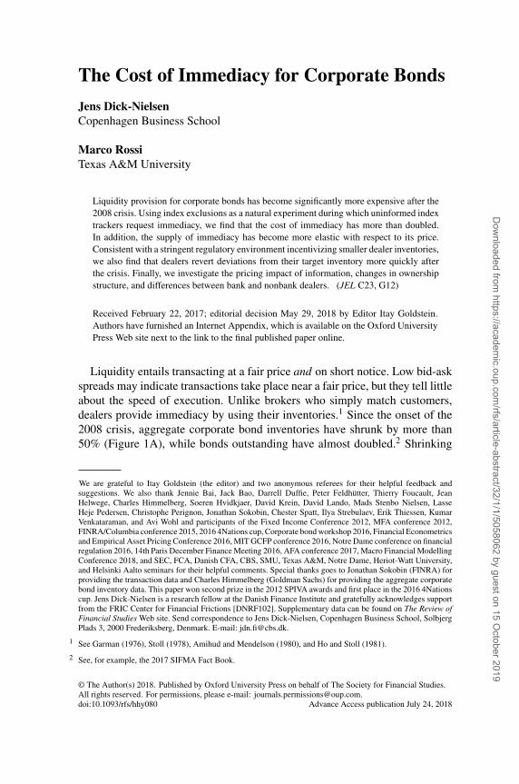
3.1 Volume dynamics at index exclusionsFigure 3 and Table 2 show that corporate bond index trackers, similar to theS&P 500 index trackers, seek to transact as close as possible to the exclusiondate. Panel A of Figure 3 shows trading volume for all bonds excluded fromthe index because of low maturity. Day 0, the event day, is the last trading dayof the month in which the bond is excluded. Trading volume is aggregatedacross all the bonds excluded during a given event and then averaged acrossall event dates. Panel B replicates panel A for bonds excluded because of arecent downgrade to speculative grade. Table 2 shows the same data used inthe figure as well as the standard error of the mean volume estimate and thetrading volume fraction relative to the day 0 volume. For both types of events,trading activity spikes on the exclusion date. Table 2 shows that the volume 20days before and after the event is only 19% to 25% of that at the event date.The peak in trading activity is thus 4 to 5 times that of the normal level.9 Asimilar trading pattern can be seen around revisions of the S&P 500 (Chen,Noronha, and Singal 2004; Harris and Gurel 1986; Shleifer 1986), the Nikkei225 (Greenwood 2005), and the FTSE 100 (Mase 2007).
Because corporate bonds trade over-the-counter, index trackers cannot becertain to transact at the desired point in time which is why activity is also highright before and after the exclusion date. Figure 3 and Table 2 show that someinvestors are tracking the index and that they seek to minimize their trackingerror, which leads to a spike in the demand for immediacy.
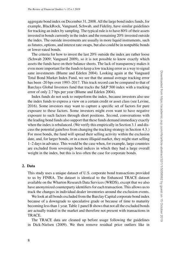
3.2 Dealer inventory around index exclusionsLet’s turn our attention to the supply of immediacy. Figure 4 shows dealerinventories for the bonds excluded from the index. The inventories arecumulative, aggregated over all dealers, and with a chosen benchmark of $0100 trading days before the event. The daily change in inventory is calculated asthe total volume in dealer buys minus the sales. For the low-maturity bonds, wesee the increase starting around 3 days prior to the exclusion date, whereas thebuildup for the downgraded bonds starts earlier but also increases in magnitudeapproximately 3 days prior to the event. The buildup in the downgraded bondsfrom day -23 to day -4 is in part caused by a buy up from the dealers on theactual downgrade date. On the downgrade date itself other investors, differentfrom index trackers, demand liquidity because many firms have an investmentpolicy that discourages holding speculative-grade assets. This sell out on thedowngrade date happens despite a grace period of up to 2 months in which theinstitutional investors are allowed to hold these bonds (see, e.g., Ambrose, Cai,and Helwege, 2012, Ellul, Jotikasthira, and Lundblad, 2011). As we will showlater, in terms of immediacy, the downgrade date is a smaller event than theexclusion date.
9 Tables A1 and A2 in the Internet Appendix show that the findings are robust to considering abnormal tradingvolume.
10
Dow
nloaded from https://academ
ic.oup.com/rfs/article-abstract/32/1/1/5058062 by guest on 15 O
ctober 2019
[17:21 17/12/2018 RFS-OP-REVF180082.tex] Page: 11 1–41
The Cost of Immediacy for Corporate Bonds
Maturity < 1 year
Event day
Av.
da
ily v
olu
me
(U
SD
mill
.)
50
10
01
50
20
0
−100 −50 0 50 100
Rating less than investment grade
Event day
Av.
da
ily v
olu
me
(U
SD
mill
.)
50
10
01
50
20
0
−100 −50 0 50 100
A
B
Figure 3Trading activity around the eventThese graphs show the average trading volume around the monthly exclusions. Panel A shows the trading volumefor the bonds excluded due to low maturity. Panel B shows those bonds excluded because of a downgrade tospeculative grade. Trading volume is aggregated across all the bonds excluded at a given event date and thenaveraged across all event dates.
After the exclusion event, Figure 4 shows that the dealers sell all or part oftheir newly acquired inventory. After 2 weeks most of the acquired inventoryof the low-maturity bonds has been sold off. For downgraded exclusions, onlyaround two-thirds of the bonds have been sold after 100 days. The two eventsthus differ in the way dealers use their inventory. Because dealers on averagedo not sell one-third of the buildup again within 100 days, the decrease in thegeneral willingness to hold inventory is expected to have affected the transactioncost of the downgraded bonds the most.
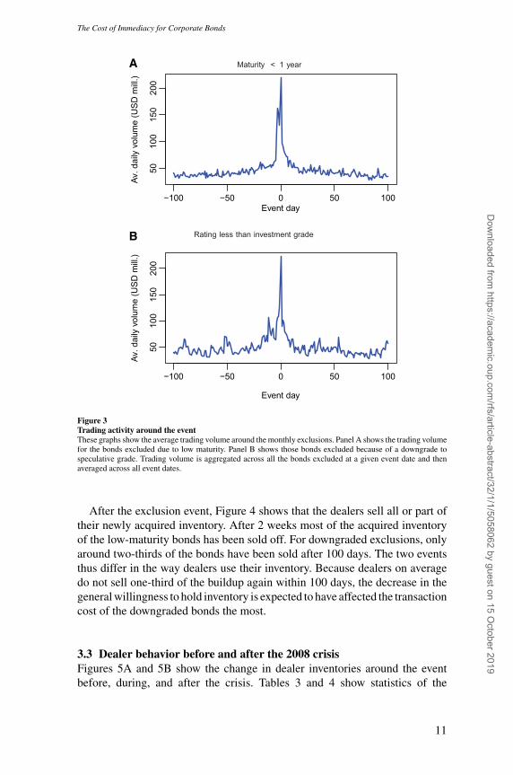
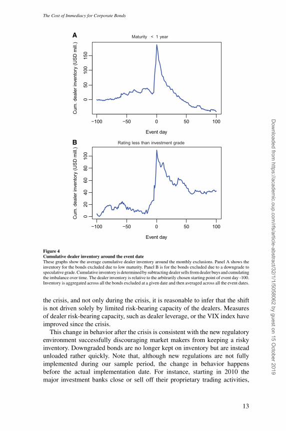
3.3 Dealer behavior before and after the 2008 crisisFigures 5A and 5B show the change in dealer inventories around the eventbefore, during, and after the crisis. Tables 3 and 4 show statistics of the
11
Dow
nloaded from https://academ
ic.oup.com/rfs/article-abstract/32/1/1/5058062 by guest on 15 O
ctober 2019

[17:21 17/12/2018 RFS-OP-REVF180082.tex] Page: 12 1–41
The Review of Financial Studies / v 32 n 1 2019
Table 2Trading activity around exclusions
Downgrade Maturity
Event time Volume SE Fraction Volume SE Fraction
−100 40.2 17.1 0.18 42.9 4.1 0.19−50 51.5 22.6 0.23 43.5 5.2 0.20−40 35.5 9.8 0.16 39.2 3.7 0.18−30 37.5 14.6 0.17 39.6 4.0 0.18−20 46.3 9.5 0.21 55.4 8.4 0.25−10 77.9 21.4 0.35 58.2 8.0 0.26−9 72.3 21.2 0.32 52.2 6.2 0.24−8 83.0 28.9 0.37 57.5 5.4 0.26−7 86.4 25.0 0.39 56.0 5.0 0.25−6 66.3 13.8 0.30 62.8 6.5 0.28−5 63.8 15.3 0.29 66.0 8.2 0.30−4 97.4 33.0 0.44 123.2 24.0 0.56−3 107.2 27.8 0.48 164.1 20.9 0.74−2 107.8 26.7 0.48 155.7 15.5 0.70−1 125.7 25.1 0.56 131.7 12.5 0.590 222.8 50.2 1.00 221.9 18.1 1.001 88.9 27.1 0.40 99.2 8.4 0.452 101.3 29.1 0.45 93.5 8.5 0.423 95.8 21.8 0.43 85.5 7.6 0.394 79.8 16.7 0.36 79.1 7.8 0.365 74.0 16.7 0.33 73.2 6.9 0.336 69.2 17.5 0.31 72.4 7.6 0.337 61.2 14.4 0.27 54.8 5.7 0.258 64.0 15.7 0.29 65.1 5.4 0.299 49.2 10.7 0.22 65.4 5.6 0.2910 64.7 18.7 0.29 52.2 4.8 0.2420 53.5 14.7 0.24 41.1 3.7 0.1930 47.4 11.6 0.21 43.4 4.4 0.2040 49.4 15.4 0.22 47.0 5.2 0.2150 50.3 13.0 0.23 40.8 4.7 0.18100 56.8 27.7 0.25 34.8 4.7 0.16
This table shows the average transaction volume around the monthly exclusions. The average is across all eventdates. Day 0 is the exclusion date. SE is the standard error of the mean transaction volume. Fraction is thetransaction volume relative to the volume at the exclusion date. Volume is measured in $millions.
corresponding inventory positions.10 The precrisis period is from 2002Q3 to2007Q2, the crisis period is from 2007Q3 to 2009Q4, and the post-crisis periodis from 2010Q1 to 2013Q4. Dealers’ behavior for the short maturity bonds haschanged from before to after the crisis in that dealers on average provide twiceas much immediacy after the crisis than before. But they decrease the inventoryto 0 over roughly the same time interval. Hence, the speed with which they selloff again has approximately doubled (we model this pattern more rigorously inthe next section).
For the downgraded bonds there is a clear shift in dealer behavior from beforeand during the crisis to after the crisis. Before and during the crisis dealers keepa large fraction of the inventory increase on their books. However, after the crisisthey only have 16% of the inventory left after 30 days compared to 58% beforethe crisis and 38% during the crisis. Because the shift in behavior happens after
10 Results are similar when looking at normalized inventory positions (see Tables A3 to A8 of the Internet Appendix.)
12
Dow
nloaded from https://academ
ic.oup.com/rfs/article-abstract/32/1/1/5058062 by guest on 15 O
ctober 2019
[17:21 17/12/2018 RFS-OP-REVF180082.tex] Page: 13 1–41
The Cost of Immediacy for Corporate Bonds
Maturity < 1 year
Event day
Cu
m.
de
ale
r in
ven
tory
(U
SD
mill
.)
05
01
00
15
0
−100 −50 0 50 100
Rating less than investment grade
Event day
Cu
m.
de
ale
r in
ven
tory
(U
SD
mill
.)
020
40
60
80
10
0
−100 −50 0 50 100
A
B
Figure 4Cumulative dealer inventory around the event dateThese graphs show the average cumulative dealer inventory around the monthly exclusions. Panel A shows theinventory for the bonds excluded due to low maturity. Panel B is for the bonds excluded due to a downgrade tospeculative grade. Cumulative inventory is determined by subtracting dealer sells from dealer buys and cumulatingthe imbalance over time. The dealer inventory is relative to the arbitrarily chosen starting point of event day -100.Inventory is aggregated across all the bonds excluded at a given date and then averaged across all the event dates.
the crisis, and not only during the crisis, it is reasonable to infer that the shiftis not driven solely by limited risk-bearing capacity of the dealers. Measuresof dealer risk-bearing capacity, such as dealer leverage, or the VIX index haveimproved since the crisis.
This change in behavior after the crisis is consistent with the new regulatoryenvironment successfully discouraging market makers from keeping a riskyinventory. Downgraded bonds are no longer kept on inventory but are insteadunloaded rather quickly. Note that, although new regulations are not fullyimplemented during our sample period, the change in behavior happensbefore the actual implementation date. For instance, starting in 2010 themajor investment banks close or sell off their proprietary trading activities,
13
Dow
nloaded from https://academ
ic.oup.com/rfs/article-abstract/32/1/1/5058062 by guest on 15 O
ctober 2019
[17:21 17/12/2018 RFS-OP-REVF180082.tex] Page: 14 1–41
The Review of Financial Studies / v 32 n 1 2019
Maturity < 1 year
Event day
Cu
m.
de
ale
r in
ven
tory
(U
SD
mill
.)
−1
00
05
01
50
25
0
−20 0 20 40 60 80 100
Precrisis
Crisis
Post−crisis
Rating less than investment grade
Event day
Cu
m.
de
ale
r in
ven
tory
(U
SD
mill
.)
05
010
01
50
−20 0 20 40 60 80 100
Precrisis
Crisis
Post−crisis
A
B
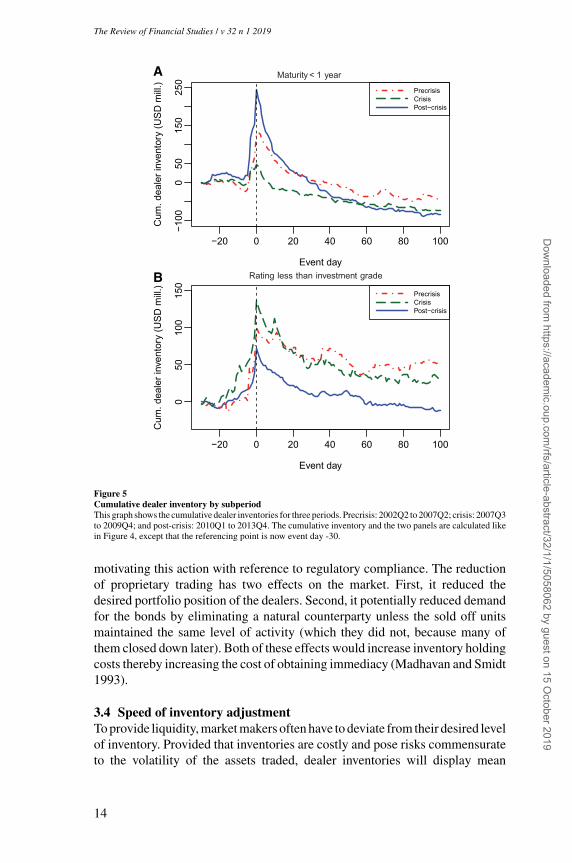
Figure 5Cumulative dealer inventory by subperiodThis graph shows the cumulative dealer inventories for three periods. Precrisis: 2002Q2 to 2007Q2; crisis: 2007Q3to 2009Q4; and post-crisis: 2010Q1 to 2013Q4. The cumulative inventory and the two panels are calculated likein Figure 4, except that the referencing point is now event day -30.
motivating this action with reference to regulatory compliance. The reductionof proprietary trading has two effects on the market. First, it reduced thedesired portfolio position of the dealers. Second, it potentially reduced demandfor the bonds by eliminating a natural counterparty unless the sold off unitsmaintained the same level of activity (which they did not, because many ofthem closed down later). Both of these effects would increase inventory holdingcosts thereby increasing the cost of obtaining immediacy (Madhavan and Smidt1993).
3.4 Speed of inventory adjustmentTo provide liquidity, market makers often have to deviate from their desired levelof inventory. Provided that inventories are costly and pose risks commensurateto the volatility of the assets traded, dealer inventories will display mean
14
Dow
nloaded from https://academ
ic.oup.com/rfs/article-abstract/32/1/1/5058062 by guest on 15 O
ctober 2019

[17:21 17/12/2018 RFS-OP-REVF180082.tex] Page: 15 1–41
The Cost of Immediacy for Corporate Bonds
Table 3Cumulative dealer inventory positions for low maturity exclusions
Precrisis Crisis Post-crisis
Event time Inventory SE Fraction Inventory SE Fraction Inventory SE Fraction
−30 −2.1 1.5 −0.02 0.5 1.8 0.01 −0.3 1.9 0.00−20 8.9 10.3 0.07 2.4 10.5 0.05 21.3 15.3 0.09−10 −10.1 12.0 −0.08 1.6 12.7 0.03 13.4 14.1 0.06−5 −18.7 12.8 −0.15 −1.2 10.7 −0.03 19.4 14.5 0.08−4 23.7 38.2 0.18 7.0 13.0 0.15 65.0 21.5 0.27−3 25.4 24.1 0.20 36.8 14.0 0.78 117.4 21.5 0.48−2 48.6 24.2 0.38 37.6 15.2 0.79 140.0 21.6 0.57−1 65.2 24.6 0.51 33.7 14.4 0.71 153.9 20.6 0.630 128.4 26.0 1.00 47.3 17.5 1.00 244.0 26.3 1.001 131.1 26.6 1.02 43.7 18.2 0.92 219.6 24.8 0.902 126.5 26.2 0.99 32.3 18.4 0.68 201.6 23.9 0.833 113.9 26.2 0.89 22.1 17.7 0.47 179.9 23.9 0.744 104.9 25.6 0.82 12.5 16.4 0.26 152.1 20.9 0.625 99.4 25.6 0.77 5.3 16.9 0.11 134.7 20.5 0.5510 57.2 26.3 0.45 −14.9 16.2 −0.31 76.5 18.6 0.3120 28.1 26.3 0.22 −21.2 18.3 −0.45 28.4 18.4 0.1230 5.8 25.8 0.04 −30.3 18.1 −0.64 −1.9 19.3 −0.0140 −1.9 29.4 −0.01 −40.4 16.6 −0.85 −31.3 19.9 −0.1350 −19.4 32.1 −0.15 −52.2 15.8 −1.10 −44.6 21.2 −0.18100 −46.2 42.3 −0.36 −72.1 15.3 −1.52 −82.9 21.5 −0.34
This table shows the average cumulative dealer inventory around the monthly exclusions because of low maturity.Cumulative inventory is found by subtracting dealer sells from dealer buys and cumulating the imbalance overtime. The dealer inventory is relative to the arbitrarily chosen starting point at event day -100. Inventory (in$millions) is aggregated across all the bonds excluded at a given date and then averaged across all the event dates.SE is the standard error of the volume mean estimate. Fraction is the inventory position relative to the position atthe exclusion date. The three time periods are 2002Q3–2007Q2, 2007Q3–2009Q4, and 2010Q1–2013Q4.
reversion. To estimate the speed of mean reversion for each dealer and eachevent, we follow Madhavan and Smidt (1993), who derive the followingequation relating inventory changes to the dealer desired level of inventory
It −It−1 =β×(It−1 −I �)+εt , (1)
where It is inventory at time t , I � is the desired level of inventory, andεt is a mean-zero unanticipated liquidity-driven volume, which is possiblyautocorrelated and heteroscedastic. In Equation (1), β ∈ (−1,0), and is morenegative when either inventory costs or the assets’ volatilities are higher.
Madhavan and Smidt (1993) show that failure to account for the time-varying nature of I � over long time periods affects the estimation of β. Whilewe consider a relatively short window around the exclusion event, we haveconditioned the sample on an event that could potentially change the desiredinventory level. Figures 4B and 5B and Tables 3 and 4 reveal that on averageinventories do not revert to zero within 100 days, suggesting that they mightsettle at a higher level after the exclusion. For this reason, we propose thefollowing specification for the desired level of inventory
I � =α0 +α11[t>−3], (2)
where α0 represents the desired level of inventory before the exclusion event,and α1 represents the change in desired inventory after exclusion. Note that we
15
Dow
nloaded from https://academ
ic.oup.com/rfs/article-abstract/32/1/1/5058062 by guest on 15 O
ctober 2019

[17:21 17/12/2018 RFS-OP-REVF180082.tex] Page: 16 1–41
The Review of Financial Studies / v 32 n 1 2019
Table 4Cumulative dealer inventory positions for downgrade exclusions
Precrisis Crisis Post-crisis
Event time Inventory SE Fraction Inventory SE Fraction Inventory SE Fraction
−30 −1.8 1.3 −0.02 −2.8 3.7 −0.02 0.3 1.8 0.00−20 −8.3 6.9 −0.08 0.8 8.3 0.01 −7.5 7.1 −0.10−10 0.3 8.6 0.00 40.9 39.0 0.30 6.1 8.8 0.08−5 2.3 9.8 0.02 52.6 44.9 0.38 17.0 7.6 0.24−4 45.8 39.4 0.46 57.9 50.3 0.42 18.5 8.9 0.26−3 36.3 23.5 0.36 59.3 51.1 0.43 21.5 8.8 0.30−2 39.6 24.9 0.40 73.2 56.1 0.53 26.2 9.9 0.36−1 56.4 25.5 0.56 87.8 60.7 0.64 38.0 10.0 0.530 99.9 35.0 1.00 137.2 83.6 1.00 72.2 16.5 1.001 92.5 31.0 0.93 127.1 77.9 0.93 64.4 14.0 0.892 89.9 31.0 0.90 119.6 74.9 0.87 55.8 11.9 0.773 85.7 30.0 0.86 119.2 75.5 0.87 53.5 11.5 0.744 85.5 30.3 0.86 109.6 69.4 0.80 48.8 11.0 0.685 84.8 30.1 0.85 103.5 67.2 0.75 49.6 11.0 0.6910 84.8 29.0 0.85 112.7 77.9 0.82 40.3 10.1 0.5620 71.6 28.1 0.72 64.9 45.7 0.47 21.7 10.0 0.3030 57.6 24.1 0.58 52.8 33.5 0.38 11.4 11.1 0.1640 70.5 31.7 0.71 53.8 35.5 0.39 9.0 9.6 0.1250 51.1 28.4 0.51 38.0 30.3 0.28 13.1 10.9 0.18100 53.7 36.6 0.54 29.9 46.1 0.22 −11.2 12.8 −0.15
This table shows the average cumulative dealer inventory around the monthly exclusions because of a downgrade.Cumulative inventory is found by subtracting dealer sells from dealer buys and cumulating the imbalance overtime. The dealer inventory is relative to the arbitrarily chosen starting point at event day -100. Inventory (in$millions) is aggregated across all the bonds excluded at a given date and then averaged across all the event dates.SE is the standard error of the volume mean estimate. Fraction is the inventory position relative to the positionat the exclusion date. The three time periods are 2002Q3–2007Q2, 2007Q3–2009Q4, and 2010Q1–2013Q4.
activate the indicator variable in Equation (2) at t −3 to account for the fact thatthe increase in inventory happening right before the event is not necessarily adeviation from an old desired level of inventory, but rather a migration toward anew desired level of inventory. We point out that activating the dummy variableat t = {−1,−2,0} makes almost no difference on estimates of β.
Our objective is to investigate whether dealers have sped up their inventorymean reversion after the 2008 crisis. To answer this question, for each event dateand for each top-five dealer, we first estimate Equation (1) with iterated GMM,using a Bartlett kernel with three lags (see Madhavan and Smidt (1993)). Todetermine top dealers we focus on the dealers that take on the most inventoryin t ∈ [−2,0] in a given event date. Note that the composition of the top dealerschanges over time. Next, we run a pooled regression with period dummiesindicating the precrisis, crisis, and post-crisis periods. Table 5 shows theseregressions for the maturity and downgrade events separately. We considerspecifications that also include time-series variables that proxy for dealers’cost of capital. The third and fourth columns present estimates for regressionsincluding dealer fixed effects. In addition to the point estimates, the first threerows of the table convert the coefficients into half-life quantities using thetransformation −log(2)/(1+β). The variables that proxy for dealers’ risk-bearing capacity are the VIX index like in Lou, Yan, and Zhang (2013) andaggregate leverage growth for broker-dealers from the Federal Reserve Flow
16
Dow
nloaded from https://academ
ic.oup.com/rfs/article-abstract/32/1/1/5058062 by guest on 15 O
ctober 2019
[17:21 17/12/2018 RFS-OP-REVF180082.tex] Page: 17 1–41
The Cost of Immediacy for Corporate Bonds
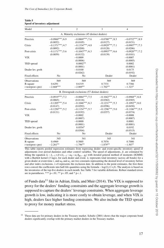
Table 5Speed of inventory adjustment
Model 1 2 3 4
A. Maturity exclusions (45 distinct dealers)
Precrisis −0.0960∗∗∗/6.9 −0.0869∗∗∗/7.6 −0.0788∗∗∗/8.5 −0.0752∗∗∗/8.9(0.0052) (0.0105) (0.0127) (0.0151)
Crisis −0.1371∗∗∗/4.7 −0.1334∗∗∗/4.8 −0.0929∗∗∗/7.1 −0.0907∗∗∗/7.3(0.0092) (0.0200) (0.0128) (0.0206)
Post-crisis −0.1171∗∗∗/5.6 −0.1043∗∗∗/6.3 −0.0993∗∗∗/6.6 −0.0920∗∗∗/7.2(0.0059) (0.0132) (0.0139) (0.0181)
VIX −0.0009 −0.0007(0.0006) (0.0005)
TED spread 0.0002∗∗ 0.0002(0.0001) (0.0001)
Dealer lev. gwth −0.0100 0.0175(0.0262) (0.0192)
Fixed effects No No Dealer Dealer
Observations 569 569 569 569R-square 0.6291 0.6319 0.7331 0.7366t-test(post<pre) −2.668∗∗∗ −2.069∗∗ −1.702∗∗ −1.323∗
B. Downgrade exclusions (57 distinct dealers)
Precrisis −0.0919∗∗∗/7.2 −0.0884∗∗∗/7.5 −0.1042∗∗∗/6.3 −0.0968∗∗/6.8(0.0065) (0.0118) (0.0382) (0.0385)
Crisis −0.1205∗∗∗/5.4 −0.1046∗∗∗/6.3 −0.1231∗∗∗/5.3 −0.1092∗∗/6.0(0.0147) (0.0292) (0.0396) (0.0450)
Post-crisis −0.1250∗∗∗/5.2 −0.1154∗∗∗/5.7 −0.1296∗∗∗/5.0 −0.1186∗∗∗/5.5(0.0131) (0.0192) (0.0357) (0.0374)
VIX −0.0002 −0.0008(0.0007) (0.0007)
TED spread −0.0000 0.0001(0.0001) (0.0001)
Dealer lev. gwth 0.0554∗ 0.0192(0.0304) (0.0315)
Fixed effects No No Dealer Dealer
Observations 345 341 345 341R-square 0.4969 0.5005 0.7076 0.7000t-test(post<pre) −2.261∗∗ −1.796∗∗ −1.879∗∗ −1.507∗This table reports pooled regression estimates from regressing dealer- and event-specific inventory speed ofadjustments over period dummies and other control variables. The speed of adjustments, β, are estimated byfitting the equation It −It−1 =β∗(It−1 −α0 −α11[t>−3]) with iterated general method of moments (IGMM)with a Bartlett kernel (3 lags), for each dealer and event. It represents total inventory (across all bonds) for agiven dealer at event-time t , and α0 and α1 are two constants representing the desired level of inventory beforeand after index exclusions. t =0 represents the exclusion date. In addition to the point estimates, the first threerows convert the coefficients into half-life quantities using the formula −log(2)/(1+β). The analysis is based onthe inventories of the top-five dealers in each month. See Table 7 for variable definitions. Robust standard errorsare in parentheses. *** p<.01; ** p<.05; and * p<.1.
of Funds data11 like in Adrian, Etula, and Muir (2014). The VIX is supposed toproxy for the dealers’ funding constraints and the aggregate leverage growth issupposed to capture the dealers’ leverage constraints. When aggregate leveragegrowth is low, indicating it is more costly to obtain leverage, and when VIX ishigh, dealers face higher funding constraints. We also include the TED spreadto proxy for money market stress.
11 These data are for primary dealers in the Treasury market. Schultz (2001) shows that the major corporate bonddealers significantly overlap with the primary market dealers in the Treasury market.
17
Dow
nloaded from https://academ
ic.oup.com/rfs/article-abstract/32/1/1/5058062 by guest on 15 O
ctober 2019

[17:21 17/12/2018 RFS-OP-REVF180082.tex] Page: 18 1–41
The Review of Financial Studies / v 32 n 1 2019
Table 5 shows a clear pattern. In both types of events, dealers display lesstolerance toward deviations from desired inventories. For instance, Column 2in panel B shows that for the typical dealer the half-life of her inventory ofbonds downgraded to speculative grade falls from 7.5 days to almost 5.5 days,a substantial 2-day difference. Note that this result is not due only to a change inthe composition of dealers over time, as it continues to hold even in regressionswith fixed effects capturing within-dealer variation. We also test whether theincrease in the speed of mean reversion is statistically significant. As can beseen from the last row of each panel, we reject the null hypothesis that thecoefficient on the post-crisis dummy is equal to the coefficient on the precrisisdummy in favor of the alternative hypothesis that the coefficient becomes morenegative after the crisis.
In their model, Madhavan and Smidt (1993) derive inventory half-life as afunction of holding costs and asset volatility. Because bond volatilities havenot increased from before to after the crisis, these results are consistent withincreased holding costs.
4. Price Dynamics
Because dealers actively use their inventories to provide liquidity to indextrackers, we expect them to earn a positive return on average as compensationfor the inventory holding costs. The following section shows that dealers arecompensated for providing liquidity. The costs are higher for the downgradeevent compared to the low-maturity event as would be expected, because thedowngraded bonds are both more risky and kept longer on inventory.
4.1 Event study of index exclusionsTable 6 shows the dealer abnormal returns for the two exclusion events.12 Eachof these returns is value-weighted either by the dealer buying volume (VW1) orby the dealer inventory buildup (VW2) on the event date and over the previous2 days. Hence, those bonds purchased by dealers that increased inventory—provided immediacy—are given more weight. Given the statistical samplingapproach to replicating the index, indexers only hold some excluded bonds. Forthis reason, equally weighted returns may mistakenly give too much weight tobonds for which traders do not seek immediacy.
Looking at Table 6, we see that the abnormal dealer returns for the bondsexcluded due to low maturity are uniformly higher after the crisis relative tobefore the crisis. Both value-weighted returns show a much sharper increase(roughly a 100%) in the cost of immediacy for highly rated, short-term bondsover the sample period. For example, at 1- and 30-day horizons, the VW2
12 In Table A9 of the Internet Appendix, we report the average intertemproal bid-ask spreads used to constructabnormal returns.
18
Dow
nloaded from https://academ
ic.oup.com/rfs/article-abstract/32/1/1/5058062 by guest on 15 O
ctober 2019

[17:21 17/12/2018 RFS-OP-REVF180082.tex] Page: 19 1–41
The Cost of Immediacy for Corporate Bonds
version shows an increase in the cost of immediacy from 6.17 and 7.50 to13.30 and 14.37, respectively.
Qualitatively, downgrade exclusions look like maturity exclusions. Quantita-tively, the returns are much larger, which is to be expected given the low ratingof these bonds and the increased inventory risk that they pose. Moreover, the
Table 6Dealer abnormal returns
Maturity exclusions Downgrade exclusions
[0,t] N EW VW1 VW2 N EW VW1 VW2
Precrisis
1 830 20.22∗∗∗ 6.34∗∗∗ 6.17∗∗∗ 243 98.19∗∗∗ 96.18∗∗∗ 81.19∗∗∗(1.58) (0.69) (0.77) (22.39) (11.80) (14.18)
2 794 20.78∗∗∗ 7.31∗∗∗ 7.13∗∗∗ 245 157.89∗∗∗ 188.18∗∗∗ 166.18∗∗∗(1.59) (0.69) (0.88) (41.48) (26.10) (32.58)
3 780 21.15∗∗∗ 7.66∗∗∗ 7.94∗∗∗ 243 160.68∗∗∗ 184.35∗∗∗ 155.62∗∗∗(1.64) (0.76) (0.84) (40.61) (24.27) (30.42)
4 777 23.03∗∗∗ 7.87∗∗∗ 8.33∗∗∗ 234 168.71∗∗∗ 195.90∗∗∗ 172.19∗∗∗(1.86) (0.99) (0.89) (34.01) (19.87) (24.40)
5 763 22.17∗∗∗ 7.59∗∗∗ 7.74∗∗∗ 229 193.42∗∗∗ 220.81∗∗∗ 196.05∗∗∗(1.69) (0.87) (1.02) (37.09) (20.18) (24.74)
10 727 21.29∗∗∗ 8.05∗∗∗ 8.20∗∗∗ 226 251.28∗∗∗ 295.58∗∗∗ 256.95∗∗∗(1.75) (1.29) (1.14) (71.83) (36.06) (48.59)
20 688 22.76∗∗∗ 7.20∗∗∗ 7.53∗∗∗ 215 173.15∗∗∗ 154.53∗∗∗ 124.79∗∗∗(2.31) (0.86) (1.10) (36.87) (17.01) (19.49)
30 675 23.22∗∗∗ 7.92∗∗∗ 7.50∗∗∗ 209 173.25∗∗∗ 174.94∗∗∗ 142.36∗∗∗(2.35) (1.11) (1.16) (63.66) (20.69) (21.05)
Crisis
1 269 46.33∗∗∗ 50.43∗∗∗ 43.02∗∗∗ 107 58.60 59.14 93.56∗(4.51) (7.51) (6.62) (43.07) (37.19) (55.86)
2 254 46.57∗∗∗ 50.86∗∗∗ 42.12∗∗∗ 101 80.74 65.61 112.61∗(5.73) (8.13) (8.22) (74.52) (51.91) (59.99)
3 236 49.80∗∗∗ 56.52∗∗∗ 52.18∗∗∗ 102 42.16 74.38 130.23∗∗∗(6.95) (9.91) (10.43) (88.86) (68.72) (17.95)
4 235 52.96∗∗∗ 56.89∗∗∗ 48.79∗∗∗ 93 50.22 118.90 174.51∗∗(6.32) (7.75) (7.69) (135.23) (123.68) (82.21)
5 230 53.18∗∗∗ 56.27∗∗∗ 47.12∗∗∗ 87 82.48 152.41 260.06∗∗(8.54) (8.86) (7.70) (157.06) (155.66) (105.61)
10 211 63.28∗∗∗ 68.71∗∗∗ 54.53∗∗∗ 91 162.46 193.45 344.43∗∗∗(8.59) (9.81) (10.72) (174.87) (145.00) (121.83)
20 211 76.35∗∗∗ 72.47∗∗∗ 54.52∗∗∗ 77 234.47 334.32∗∗ 492.31∗∗∗(13.67) (16.76) (17.55) (203.77) (169.83) (173.18)
30 206 96.55∗∗∗ 102.75∗∗∗ 80.71∗∗∗ 71 −139.2 270.88∗ 373.44∗∗∗(20.74) (26.35) (22.95) (381.10) (164.37) (118.32)
Post-crisis
1 1,085 26.27∗∗∗ 13.53∗∗∗ 13.30∗∗∗ 213 99.91 292.93∗∗∗ 294.79∗∗∗(2.06) (1.64) (1.56) (87.86) (110.71) (103.68)
2 1,054 27.16∗∗∗ 13.79∗∗∗ 13.59∗∗∗ 208 149.92∗ 350.12∗∗∗ 366.33∗∗∗(1.98) (1.39) (1.34) (85.42) (125.27) (115.78)
3 1,041 26.47∗∗∗ 13.25∗∗∗ 13.06∗∗∗ 193 185.00∗ 488.51∗∗∗ 508.88∗∗∗(2.06) (1.31) (1.29) (109.72) (174.48) (167.24)
4 995 29.46∗∗∗ 13.99∗∗∗ 13.62∗∗∗ 185 203.06 577.79∗∗∗ 592.19∗∗∗(2.41) (1.62) (1.56) (128.18) (204.04) (192.88)
5 990 30.06∗∗∗ 14.35∗∗∗ 14.08∗∗∗ 188 231.84 651.57∗∗∗ 682.85∗∗∗(2.45) (1.84) (1.79) (145.41) (218.76) (212.84)
10 954 30.19∗∗∗ 14.87∗∗∗ 14.46∗∗∗ 177 173.39∗ 381.56∗∗∗ 444.73∗∗∗(2.26) (1.61) (1.57) (101.57) (146.80) (157.25)
19
Dow
nloaded from https://academ
ic.oup.com/rfs/article-abstract/32/1/1/5058062 by guest on 15 O
ctober 2019

[17:21 17/12/2018 RFS-OP-REVF180082.tex] Page: 20 1–41
The Review of Financial Studies / v 32 n 1 2019
Table 6Continued
Maturity exclusions Downgrade exclusions
[0,t] N EW VW1 VW2 N EW VW1 VW2
20 861 34.06∗∗∗ 15.93∗∗∗ 16.02∗∗∗ 175 314.30 807.29∗∗∗ 869.89∗∗∗(3.25) (1.67) (1.74) (193.71) (281.61) (258.22)
30 814 34.20∗∗∗ 15.09∗∗∗ 14.37∗∗∗ 163 332.27 937.37∗∗∗ 965.48∗∗∗(3.29) (1.60) (1.65) (229.68) (313.65) (310.50)
This table shows the dealer-bond specific average returns of bonds excluded from the Barclay Corporate BondIndex because of low maturity. Returns are calculated as log price changes between day 0 (the exclusion date)and day t after exclusion. The returns are calculated from the dealer’s perspective. First, the intertemporal bid-askspread is calculated using the dealer-buy price (dealer-specific average buy price over days -2,-1, and 0) and theaverage dealer sell price at day t (average across all dealers). Second, the abnormal return is the intertemporal bid-ask spread minus the return on a matched portfolio. The portfolio is matched on rating and time to maturity. VW1is weighted by the aggregate buying volume in the specific cusip for all dealers with a positive inventory buildupin the bond. VW2 is weighted by the aggregate inventory buildup for dealers with a net positive inventory changebetween day -3 and 0. The three time periods are 2002Q3–2007Q2, 2007Q3–2009Q4, and 2010Q1–2013Q4.*** p<.01; ** p<.05; and * p<.1.
increase in the cost of immediacy because the precrisis period is much largerthan the maturity exclusion case. As can be seen from the last two columns,the increase ranges from more than 200% at the 1-day horizon (e.g., 81.19 to294.79 for VW2) to more than 500% at the 30-day horizon (e.g., 142.36 to965.48 for VW2).
4.2 Regression analysis of the cost of immediacyTable 6 shows a remarkable increase in the price of immediacy since the onsetof the 2008 crisis. Next, we relate the higher returns earned by dealers to thequantity of bonds transacted, and other variables likely to affect the supply anddemand of immediacy. Generally, the price (p) and quantity (q) of immediacyare jointly determined in the market. Therefore regressing the compensation forimmediacy on its quantity subjects the econometrician to simultaneous equationbias. Importantly, we do not usually know whether such regression estimatesa supply function or a demand function. More formally, a suitable empiricalmodel to consider would be:
qDt = α0 +α1pt +et (3)
qSt = β0 +β1pt +ut (4)
qDt = qS
t =qt , (5)
where et , ut contain both observable and unobservable demand and supplyshifters, and the last equation imposes market clearing. To obtain unbiased andconsistent estimates of the slopes, a two-stage least squares (2SLS) is normallyused.13 However, this is not necessary in our setting, which provides a naturalidentifying restriction.
13 See Choi et al. (2010) for a recent application of this methodology to the analysis of issue proceeds andunderpricing for convertible bonds.
20
Dow
nloaded from https://academ
ic.oup.com/rfs/article-abstract/32/1/1/5058062 by guest on 15 O
ctober 2019

[17:21 17/12/2018 RFS-OP-REVF180082.tex] Page: 21 1–41
The Cost of Immediacy for Corporate Bonds
The premise of this study is that indexers are impatient around bond exclusionevents. Our empirical analysis so far suggests that their price demand elasticityaround these events is extremely low. Therefore, the identifying restriction thatwe impose is α1 =0 in Equation (3).14 This restriction identifies the empiricalrelation between prices and quantities as a supply relation, so a nonnegativerelation between prices and quantities in our data would provide support forour assumption.
4.2.1 Model specification. The dependent variable in the regressions is thecumulative abnormal bond returns (a proxy for the cost of immediacy, i.e.,p(q)). The independent variable of interest is a measure of liquidity provision(q). Assuming that dealers see the excluded bonds as reasonable substitutes, wedefine q as the aggregate dealer inventory imbalance (measured in millions ofdollars) for each dealer from day -2 to 0 across all excluded bonds at the event(downgrade and maturity separately). We drop all dealers with a net negativeinventory imbalance. We interact q with three dummies indicating whether theobservation takes place before, during, or after the 2008 crisis.
We expect our specification to capture a nonnegative supply relation betweenthe price and the quantity of immediacy. To this end, it is important to accountfor potential demand-side shifters likely to affect the price of immediacy. Itis reasonable to assume that a large event, that is, an event during which alarge portion of the index is reconstituted, is more likely to result in a higherdemand of immediacy. For this reason, in our baseline regression we include thepercentage of the index excluded each month as a control variable. In subsequentregressions, we control for additional demand shifters, such as the demand forimmediacy coming from buy-side institutions around index exclusions.
We also include other factors likely to influence the cost of immediacy.Specifically, we include the amount outstanding of the bond. Larger bondsare likely more transparent and liquid than smaller bonds and are thereforeless risky to have on inventory. We include the variables proxying for dealers’risk-bearing capacity which we also used in the inventory half-life regression.Finally, we include industry (financials vs. nonfinancials), rating, and perioddummies that are interacted with each other. Lastly, we also include dealer fixedeffects. To save space, we have not reported the estimated coefficients on thedummies in the regression tables.
Table 7 provides descriptive statistics on the variables used in the regressions.
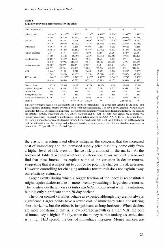
4.2.2 Cost of immediacy before and after the crisis. Table 8 reports thecoefficient estimates of the regressions. As can be seen from the table, theprice of providing liquidity is increasing in the amount of liquidity transacted,
14 Chacko, Jurek, and Stafford (2008) impose a similar restriction in their theoretical model of the price ofimmediacy, but do so in the context of a limit order book.
21
Dow
nloaded from https://academ
ic.oup.com/rfs/article-abstract/32/1/1/5058062 by guest on 15 O
ctober 2019

[17:21 17/12/2018 RFS-OP-REVF180082.tex] Page: 22 1–41
The Review of Financial Studies / v 32 n 1 2019
Table 7Descriptive statistics of regression variables
Event Variable Obs. Mean SD p25 p50 p75
All TED spread 131 45.37 60.47 17.00 24.00 44.00All VIX 131 20.40 8.91 14.38 17.74 23.70All Dealer lev. gwth 131 −0.01 0.21 −0.05 0.02 0.05All % idx excluded 131 1.15 1.17 0.74 0.91 1.21All Issue size (MIO) 3,314 664.91 569.02 300.00 500.00 750.00All Dealer inv. (q) 3,314 4.62 13.69 0.00 0.06 2.93All Log issue size 3,314 17.75 0.68 17.24 17.71 18.18All Ins. change (pct) 3,230 −0.01 0.03 −0.01 0.00 0.00All MF change (pct) 3,230 −0.01 0.03 −0.01 −0.00 0.00All Stk ret (excl.) 2,119 0.00 0.07 −0.02 0.01 0.03
Downgrd Issue size (MIO) 695 655.59 593.82 300.00 500.00 750.00Downgrd Dealer inv. (q) 695 3.86 13.11 0.00 0.00 1.91Downgrd Log issue size 695 17.57 0.75 17.07 17.46 18.02Downgrd Ins. change (pct) 687 −0.02 0.06 −0.03 −0.00 0.00Downgrd MF change (pct) 687 −0.00 0.03 −0.01 0.00 0.00Downgrd Stk ret (excl.) 461 −0.00 0.08 −0.04 0.00 0.04
Maturity Issue size (MIO) 2,619 667.38 562.35 300.00 500.00 750.00Maturity Dealer inv. (q) 2,619 4.82 13.83 0.00 0.08 3.27Maturity Log Issue Size 2,619 17.80 0.65 17.25 17.73 18.19Maturity Ins. change (pct) 2,543 −0.01 0.02 −0.01 0.00 0.00Maturity MF change (pct) 2,543 −0.01 0.02 −0.01 −0.00 0.00Maturity Stk ret (excl.) 1,658 0.00 0.06 −0.02 0.01 0.03
This table presents descriptive statistics for the variables used in the regression analysis. The statistics is dividedinto the whole sample, the downgrade sample, and the low-maturity sample. The TED spread is the differencebetween the 3-month LIBOR rate and the 3-month Treasury-bill rate. VIX is the CBOR volatility index derivedfrom the implied volatility on S&P 500 index options. Issue size is the offering amount for the bond in millions.Dealer lev gwth is the aggregate leverage growth for broker-dealers obtained from the Federal Reserve Flow ofFunds data. Pct idx excluded is the percentage of the index being reconstituted. q is the dealer-specific aggregateimbalance. MF change (pct) and INS change (pct) are, respectively, mutual funds’ and insurance companies’percentage changes in ownership of an excluded bond. Bond ownership data come from Lipper eMAXX. Stk ret(excl.) is the issuer stock return at exclusion.
making the relation reminiscent of a supply curve. Comparing the interactionof q with the post-crisis dummy to the interaction of q with the precrisisdummy reveals that the supply curve is relatively steeper after the crisis.15
This result suggests that providing immediacy has become more costly after thecrisis, and, consequently, dealers require higher returns for providing additionalimmediacy. The results on the effect of q are also economically significant.Noting that the returns are measured in basis points, a one standard deviationchange in q after the crisis ($16.5 million) is roughly associated with anadditional 18.5 bps of return over 3 days and 35 (16.5×2.10) bps over a 20-day horizon. The coefficient on the precrisis interaction is statistically andeconomically insignificant at all horizons, indicating that dealers’ strategy tobuy and temporarily hold excluded bonds could easily scale up.
The regressions include interacted fixed effects, which capture the fact thatbonds with the same rating might be priced differently before, during, and after
15 We conduct t-tests of the difference in coefficients and find that the difference is generally statistically significantat conventional levels.
22
Dow
nloaded from https://academ
ic.oup.com/rfs/article-abstract/32/1/1/5058062 by guest on 15 O
ctober 2019
[17:21 17/12/2018 RFS-OP-REVF180082.tex] Page: 23 1–41
The Cost of Immediacy for Corporate Bonds
Table 8Liquidity provision before and after the crisis
Event window: (0,t] 1 2 3 4 5 10 20 30
q*Post-crisis 0.630∗∗ 0.821∗∗∗ 1.122∗∗ 1.329∗∗ 1.629∗∗ 0.776∗ 2.103∗∗∗ 1.887∗∗(0.308) (0.310) (0.471) (0.582) (0.683) (0.403) (0.699) (0.789)
q*Crisis 0.928 0.741 1.449 2.699∗ 3.725∗∗ 2.970∗ 4.904∗∗∗ 8.461∗∗(0.776) (0.980) (1.033) (1.417) (1.577) (1.699) (1.561) (3.980)
q*Precrisis 0.0617 0.180 0.130 0.190 0.217 0.255 0.0426 0.119(0.0874) (0.126) (0.117) (0.167) (0.142) (0.193) (0.129) (0.240)
Pct idx excluded 3.977 12.17 9.541 6.500 10.25 20.26 12.72∗∗ 20.85(4.006) (8.352) (8.054) (6.267) (7.560) (12.85) (5.938) (13.12)
Log Issue Size −15.16∗∗ −18.44∗∗ −13.04 −7.045 −14.60 −9.497 −14.91 9.723(6.610) (8.790) (11.08) (12.54) (14.19) (17.98) (16.49) (21.25)
Dealer lev. gwth −90.08∗ −94.07∗ −122.4∗ −89.27 −138.0 −101.2 −147.5 −236.6∗∗(48.55) (49.74) (64.70) (73.04) (85.26) (90.99) (110.9) (114.9)
VIX 2.446∗ 2.199 2.510 2.630 2.320 1.786 5.328∗ 5.237∗(1.345) (1.429) (1.865) (2.123) (2.294) (1.995) (2.852) (2.984)
TED spread 1.066∗∗ 1.220∗∗∗ 1.743∗∗∗ 1.832∗∗ 1.833∗∗ 1.346∗∗ 1.774∗ 2.139∗(0.416) (0.450) (0.593) (0.721) (0.816) (0.673) (0.966) (1.112)
Observations 15,713 15,338 14,993 14,779 14,634 14,101 13,401 12,919Adjusted R-squared 0.219 0.249 0.261 0.257 0.286 0.252 0.368 0.341Dealer FEs Yes Yes Yes Yes Yes Yes Yes YesRating*Period FEs Yes Yes Yes Yes Yes Yes Yes YesF-test (FE interactions) 67.46 11.57 6.717 2.592 13.76 57.92 3.935 16.77Prob>F 0 0 3.86×10⁻¹⁰ 0.00249 0 0 2.18×10-05 0
This table presents regression coefficients for a series of regressions. The dependent variable is the bond- anddealer-specific abnormal returns over the period from the exclusion day 0 to day t after exclusion. Variables aredefined in Table 7. The regressions include (interacted) period/industry/rating and dealer fixed effects. The periodsare 2002Q3–2007Q2 (precrisis), 2007Q3–2009Q4 (crisis), and 2010Q1–2013Q4 (post-crisis). We consider twoindustry categories (financial vs. nonfinancial) and six rating categories (AAA–AA, A, BBB, BB, B, and CCC–C). Robust standard errors are clustered at the bond issuer and event date level. An F-test tests the null hypothesisthat the interactions of the ratings and subperiod fixed effects are jointly zero. Robust standard errors are inparentheses. *** p<.01; ** p<.05; and * p<.1.
the crisis. Interacting fixed effects mitigates the concerns that the increasedcost of immediacy and the increased supply price elasticity come only froma higher level of risk aversion (hence risk premiums) in the market. At thebottom of Table 8, we test whether the interaction terms are jointly zero andfind that these interactions explain some of the variation in dealer returns,suggesting that it is important to control for potential changes in risk aversion.However, controlling for changing attitudes toward risk does not explain awayour elasticity estimates.
Larger events during which a bigger fraction of the index is reconstitutedmight require dealers to take on more inventory resulting in larger dealer returns.The positive coefficient on Pct Index Excluded is consistent with this intuition,but it is only significant at the 20-day horizon.
The other control variables behave as expected although they are not alwayssignificant. Larger bonds have a lower cost of immediacy when consideringshort horizons, but the effect is insignificant at long horizons. When dealersare more constrained, that is, a low leverage growth or a high VIX, the costof immediacy is higher. Finally, when the money market undergoes stress, thatis, a high TED spread, the cost of immediacy increases. Money markets are
23
Dow
nloaded from https://academ
ic.oup.com/rfs/article-abstract/32/1/1/5058062 by guest on 15 O
ctober 2019
[17:21 17/12/2018 RFS-OP-REVF180082.tex] Page: 24 1–41
The Review of Financial Studies / v 32 n 1 2019
important for market makers, because they often fund their market makingactivity through repo transactions.
4.3 The hidden cost of bond index investmentThe cost of immediacy includes a price pressure component as well as thebid-ask spread. From the perspective of the institutional investor, the pricepressure component is the more interesting part (Hendershott and Menkveld2014). Because the bid-ask spread or the half-spread is in some sense a sunkcost once the investor owns the asset and wants to sell, variation in the dealer’sbuying price is what constitutes the true opportunity cost. Table 9 shows theabnormal event return calculated like in Table 6 but using only dealer buy prices.This is thus the return that the institutional investor could have gotten (all elseequal) had she waited to sell instead of selling at the event date. The negative t’sindicate the return from before the exclusion date and up to the exclusion event.A negative return before the exclusion date thus means that the price decreasedleading up to the event. From Table 9, we see that for the maturity exclusionsthe bid price decreases leading up to the exclusion and it also decreases afterexclusion. The dealer return from Table 6 is therefore driven by an increasein the bid-ask spread rather than a rebound of the price. For the downgradeexclusions, the bid price decreases leading up to the event and increases afterthe event, indicating that much of the dealer return from these exclusions aregenerated by a rebound of the price level.
The bid-to-bid returns pick up a hidden cost of index tracking (see, e.g.,Chen, Noronha, and Singal, 2006, Pedersen, 2018, Petajisto, 2011). To seethis, consider that the bond index return is calculated using the average pricefrom day 0 and that this price will be heavily depressed by the concentratedselling from index trackers. Although index trackers obtain potentially a zerotracking error by trading on the exclusion date, the actual returns attained arebased on severely discounted prices. It is in principle possible to outperformthe index on average by avoiding the price pressure and selling several daysaway from the rebalancing date.
On average 1.2% of the index (in market values) is excluded each month.Using a back of the envelope calculation, the hidden cost of index tracking isthe average (monthly) abnormal bid-to-bid exclusion return times the fractionexcluded from the index (multiplying by 12 gives a rough estimate of the annualcosts). The ratio of low- maturity exclusions to downgrade exclusion is usually3:1 (in market values). For downgraded bonds it is optimal to sell out 30 daysafter the event, whereas for maturity exclusions it is optimal to sell out 10 daysbefore the event according to Table 9. The hidden cost of index tracking is thusroughly 0.012×12×(0.25×0.0966+0.75×0.00129)=34 bps.
The cost estimate can be compared to the hidden cost from stock indexinvestment calculated in Petajisto (2011) of 21–28 bps annually for the S&P500. Note that this annual cost estimate is only indicative, because we do not
24
Dow
nloaded from https://academ
ic.oup.com/rfs/article-abstract/32/1/1/5058062 by guest on 15 O
ctober 2019

[17:21 17/12/2018 RFS-OP-REVF180082.tex] Page: 25 1–41
The Cost of Immediacy for Corporate Bonds
Table 9Bid-to-bid returns and the hidden cost of indexing
Maturity exclusions Downgrade exclusions
[0,t] N EW VW1 VW2 N EW VW1 VW2
Intertemporal bid-ask spreads
−10 888 −15.04∗∗∗ −7.20∗∗ −6.66∗∗ 179 −236.2∗∗ −357.3∗∗ −349.3∗∗(2.83) (2.89) (3.03) (112.38) (153.68) (143.63)
−5 973 −10.41∗∗∗ −2.91 −2.96 198 −286.9∗∗ −216.4∗∗∗ −196.3∗∗(2.20) (1.90) (2.03) (132.66) (75.00) (92.02)
−4 1,059 −9.56∗∗∗ −1.77 −1.70 192 −217.0∗ −117.1∗∗∗ −87.04∗(2.09) (1.64) (1.65) (127.68) (42.04) (47.91)
−3 1,216 −7.86∗∗∗ −1.28 −1.68 202 −190.0 −111.4∗∗ −87.19(2.24) (1.78) (1.65) (123.68) (48.42) (61.57)
1 947 5.87∗∗∗ −2.01∗ −2.40∗ 208 83.49 380.83∗∗ 404.00∗∗(1.65) (1.13) (1.36) (118.02) (167.58) (161.34)
2 911 5.60∗∗∗ −2.13∗ −2.63∗∗ 214 158.80 488.26∗∗ 515.44∗∗∗(1.73) (1.13) (1.27) (130.18) (197.33) (189.08)
3 904 6.37∗∗∗ −1.05 −1.46 204 210.10 621.78∗∗ 662.27∗∗∗(1.56) (0.99) (1.13) (161.63) (253.37) (256.40)
4 885 7.29∗∗∗ −1.28 −1.34 188 231.39 736.97∗∗ 756.72∗∗(1.30) (1.02) (1.17) (192.10) (304.91) (314.49)
5 880 8.34∗∗∗ −1.96∗ −2.53∗∗ 181 264.08 830.50∗∗ 883.80∗∗(1.48) (1.15) (1.28) (220.66) (343.04) (349.79)
10 895 13.16∗∗∗ 1.15 1.02 174 131.33 475.54∗∗ 577.63∗∗(2.50) (1.96) (2.11) (147.23) (218.24) (241.65)
20 871 18.79∗∗∗ 4.16 3.61 166 357.55 1043.1∗∗∗ 1124.7∗∗∗(3.36) (2.79) (2.56) (301.68) (373.96) (358.72)
30 832 23.88∗∗∗ 7.10∗∗ 6.02∗∗ 174 524.61 1406.5∗∗∗ 1439.4∗∗∗(4.40) (3.02) (2.87) (355.04) (443.29) (421.69)
Abnormal returns
-10 888 −21.61∗∗∗ −13.00∗∗∗ −12.91∗∗∗ 179 −322.3∗∗ −566.6∗∗ −530.1∗∗(2.03) (2.00) (2.03) (152.23) (257.04) (257.97)
-5 973 −15.35∗∗∗ −7.64∗∗∗ −7.78∗∗∗ 198 −354.9∗∗ −385.2∗∗ −363.3∗∗(1.32) (1.32) (1.48) (154.12) (153.03) (169.78)
-4 1,059 −14.44∗∗∗ −6.66∗∗∗ −6.86∗∗∗ 192 −290.3∗∗ −293.7∗∗ −262.8∗∗(1.50) (1.24) (1.18) (146.19) (121.61) (127.92)
-3 1,216 −12.01∗∗∗ −5.12∗∗∗ −5.65∗∗∗ 202 −262.7∗ −287.9∗∗ −259.6∗(1.82) (1.33) (1.06) (144.22) (119.64) (135.19)
1 947 4.89∗∗∗ −2.60∗∗∗ −2.76∗∗∗ 208 55.66 304.63∗∗ 324.98∗∗(1.65) (0.80) (0.91) (100.57) (136.67) (133.71)
2 911 3.77∗∗ −3.51∗∗∗ −3.78∗∗∗ 214 110.44 358.86∗∗ 384.37∗∗∗(1.52) (0.69) (0.68) (100.82) (146.05) (142.49)
3 904 3.94∗∗∗ −3.05∗∗∗ −3.25∗∗∗ 204 149.10 463.94∗∗ 504.06∗∗∗(1.49) (0.76) (0.82) (124.28) (188.31) (195.66)
4 885 4.14∗∗∗ −3.73∗∗∗ −3.49∗∗∗ 188 167.47 563.32∗∗ 594.10∗∗(1.29) (0.82) (0.83) (146.60) (224.34) (234.20)
5 880 4.61∗∗∗ −4.75∗∗∗ −5.10∗∗∗ 181 198.02 647.02∗∗ 700.37∗∗∗(1.26) (0.88) (0.94) (173.08) (262.52) (268.95)
10 895 7.00∗∗∗ −3.35∗∗ −3.17∗∗ 174 105.16 438.89∗∗ 539.66∗∗(1.86) (1.35) (1.51) (135.07) (198.27) (215.33)
20 871 8.59∗∗∗ −2.46∗∗ −2.28 166 264.48 781.47∗∗∗ 847.64∗∗∗(2.06) (1.22) (1.40) (231.05) (287.87) (283.36)
30 832 6.83∗∗∗ −5.27∗∗∗ −5.21∗∗∗ 174 312.39 935.26∗∗∗ 966.08∗∗∗(2.21) (1.34) (1.43) (257.10) (315.03) (305.35)
This table replicates Table 6, except that the time ±t price is an average (across all dealers) of the buy price. Fornegative t , we compute bid returns from −t to 0; for positive t , we compute bid returns from 0 to t . Consistentwith Table 6, prices at time zero are dealer specific. Returns are only calculated for the most recent time period.*** p<.01; ** p<.05; and * p<.1.
25
Dow
nloaded from https://academ
ic.oup.com/rfs/article-abstract/32/1/1/5058062 by guest on 15 O
ctober 2019

[17:21 17/12/2018 RFS-OP-REVF180082.tex] Page: 26 1–41
The Review of Financial Studies / v 32 n 1 2019
consider what would happen dynamically when volumes are redistributed awayfrom the exclusion date.
The hidden cost of index tracking raises the question why index trackersdo not deviate from trading at the rebalancing date. To illustrate this, we lookat the Vanguard Total Bond Market Index Fund as an example. The BarclayCapital Corporate Bond Market Index constitutes around one third of theindex that the Vanguard fund is tracking. The Vanguard fund had an averageyearly tracking error of -20 bps over 1993-2017. The tracking error primarilycomes from transaction costs and management fees. Following the strategyfrom above (using intertemporal returns) and selling out 10 days before theevent for maturity exclusions and 30 days after the event day for downgradeexclusions, the Vanguard fund could improve its tracking error by between 3–9 bps, depending on our assumptions about how the fund samples the index.However, the improvement in tracking error comes with an increase in thestandard deviation of the tracking error, which increases from 20.0 bps to 20.5bps. Hence, there is a trade-off between size and stability of the tracking error.Thus, the strategy of selling out very close to the exclusion date could beexplained by a desire to keep the tracking risk low.
Although the increase in tracking error variance that we calculate may seemmodest, the fund could have a fear of realizing a very large negative event, whichwould cause additional variation in the tracking error. This dislike for trackingrisk also could be seen in 2002, when the Vanguard fund underperformed thebenchmark by 2.00%. This lead the fund to change its tracking strategy froma strategy that used to overweight some sectors. In the semiannual report fromJune 2002, fund managers stated that they would make this change despite theirbelief that the overweighting had rewarded them over the long run. Aversion tosuch tail risk is consistent with findings that the flow-to-performance relationfor corporate bond funds is concave (Goldstein, Jiang, and Ng 2017).
5. Exploring Additional Channels
5.1 Evolution of bond ownership structureThe discussion so far has ignored changes in the market structure that couldpotentially affect the price of immediacy. Based on data from the LippereMaxx institutional bond database, Table 10 and Figure 6 show that mutualfund investors have risen in importance in both relative and absolute terms.Figure 6 further shows that high-yield funds, which can be seen as naturalbuyers for bonds that exit an investment-grade index to join a high-yieldindex, have also risen in importance, but have grown less than other mutualfunds. Table 10 reports absolute and relative frequencies (by subperiod) offund*quarter observations in the Lipper eMaxx database. As can be seen,insurance companies are a major player in the corporate bond market. However,mutual funds have gained importance in this space. While before the crisisholding reports by mutual funds represent about a third of insurance company
26
Dow
nloaded from https://academ
ic.oup.com/rfs/article-abstract/32/1/1/5058062 by guest on 15 O
ctober 2019

[17:21 17/12/2018 RFS-OP-REVF180082.tex] Page: 27 1–41
The Cost of Immediacy for Corporate Bonds
Table 10Distribution of investment categories over time
Period Freq. Insurance Mut. F. Pens. F. Annuities Other
Precrisis Count 33,879 11,686 1,255 2,693 482% 28.65% 9.88% 1.06% 2.28% 0.41%
Crisis Count 10,894 5,643 163 1,364 281% 9.21% 4.77% 0.14% 1.15% 0.24%
Post-crisis Count 28,100 16,490 305 4,053 975% 23.76% 13.94% 0.26% 3.43% 0.82%
This table reports the absolute and relative frequencies of the investment categories represented in the LippereMAXX institutional Bond holdings database. The observations for which the frequencies are computed are atthe fund*date level.
Pa
r a
mo
un
t (U
SD
bn
)
02
00
40
06
00
80
01
,00
0
2003Q1 2005Q1 2007Q1 2009Q1 2011Q1 2013Q1
Total par amount
Spec. par amount
Figure 6Mutual fund growthThe figure shows the total bond par value held by mutual funds covered by Lipper eMAXX. The other line reportsholdings by mutual funds specializing in speculative-grade bonds.
reports, after the crisis their number has grown to be more than half. Othertypes of investors are negligible, so we ignore them going forward.
Next, we explore how mutual funds and insurance companies trade aroundexclusion events. Figure 7 shows that, compared to the crisis, mutual fundshold a much larger share of excluded bonds. This figure shows the percentageof bonds held by insurance companies and mutual funds before and soonafter the exclusion event and provides prima facie evidence of the tradingdirection of these corporate bond investors around the exclusion event. As canbe seen, insurance companies (left graphs) reduce their holdings, especiallyfor downgrade exclusions (Figure 7C). In addition to showing the increasedrelevance of mutual funds, Figures 7B and 7D show that mutual funds werenet buyers of excluded bonds before the crisis, and have become net sellerssince. This change in behavior by mutual funds apparently contrasts the resultsin Choi and Huh (2017), who suggest that some liquidity provision is providedby nondealers after the crisis. A related paper by Anand, Jotikasthira, andVenkataraman (2017) is more consistent with our study in that it suggests that,
27
Dow
nloaded from https://academ
ic.oup.com/rfs/article-abstract/32/1/1/5058062 by guest on 15 O
ctober 2019
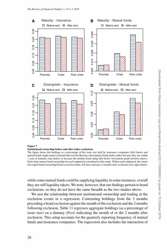
[17:21 17/12/2018 RFS-OP-REVF180082.tex] Page: 28 1–41
The Review of Financial Studies / v 32 n 1 2019
A B
C D
0.00
0.06
0.12
0.18
0.24
0.30
Precrisis Crisis Post−crisis
Before excl. After excl.0.
000.
030.
060.
090.
12
Precrisis Crisis Post−crisis
Before excl. After excl.
0.00
0.06
0.12
0.18
0.24
0.30
Precrisis Crisis Post−crisis
Before excl. After excl.
0.00
00.
015
0.03
00.
045
0.06
0
Precrisis Crisis Post−crisis
Before excl. After excl.
Maturity - Insurance Maturity - Mutual funds
Downgrade - Insurance Downgrade - Mutual funds
Figure 7Institutional ownership before and after index exclusionsThe figure shows the holdings as a percentage of the issue size held by insurance companies (left charts) andmutual funds (right charts) in bonds that exit the Barclays Investment-Grade Index either because they are within1 year of maturity (top charts) or because the median bond rating falls below investment grade (bottom charts).Each chart reports bond ownership for each subperiod considered in this study. Within each subperiod, the chartsalso report bond ownership before exclusion (blue, left bars) and up to 2 months after exclusion (red, right charts).
while some mutual funds could be supplying liquidity in some instances, overallthey are still liquidity takers. We note, however, that our findings pertain to bondexclusions, so they do not have the same breadth as the two studies above.
We test the relationship between institutional ownership and trading at theexclusion events in a regression. Contrasting holdings from the 3 monthspreceding a bond exclusion against the month of the exclusion and the 2 monthsfollowing exclusion, Table 11 regresses aggregate holdings (as a percentage ofissue size) on a dummy (Post) indicating the month of or the 2 months afterexclusion. This setup accounts for the quarterly reporting frequency of mutualfunds and insurance companies. The regression also includes the interaction of
28
Dow
nloaded from https://academ
ic.oup.com/rfs/article-abstract/32/1/1/5058062 by guest on 15 O
ctober 2019
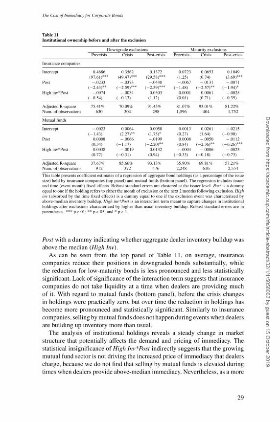
[17:21 17/12/2018 RFS-OP-REVF180082.tex] Page: 29 1–41
The Cost of Immediacy for Corporate Bonds
Table 11Institutional ownership before and after the exclusion
Downgrade exclusions Maturity exclusionsPrecrisis Crisis Post-crisis Precrisis Crisis Post-crisis
Insurance companies
Intercept 0.4686 0.3562 0.1372 0.0723 0.0653 0.1049(97.61)∗∗∗ (49.47)∗∗∗ (29.58)∗∗∗ (1.25) (0.74) (3.69)∗∗∗
Post −.0233 −.0373 −.0440 −.0067 −.0131 −.0071(−2.43)∗∗ (−2.59)∗∗∗ (−2.59)∗∗∗ (−1.48) (−2.57)∗∗ (−1.94)∗
High inv*Post −.0074 −.0034 0.0303 0.0001 0.0061 −.0025(−0.54) (−0.13) (1.12) (0.01) (0.71) (−0.35)
Adjusted R-square 75.41% 70.09% 91.45% 81.07% 93.01% 81.22%Num. of observations 630 304 298 1,596 404 1,752
Mutual funds
Intercept −.0023 0.0064 0.0058 0.0013 0.0261 −.0215(−1.43) (2.27)∗∗ (1.75)∗ (0.27) (1.64) (−0.90)
Post 0.0008 −.0066 −.0199 0.0008 −.0050 −.0112(0.34) (−1.17) (−2.20)∗∗ (0.84) (−2.36)∗∗ (−6.26)∗∗∗
High inv*Post 0.0038 −.0019 0.0132 −.0004 −.0006 −.0023(0.77) (−0.31) (0.94) (−0.33) (−0.18) (−0.73)
Adjusted R-square 37.67% 85.66% 93.13% 35.90% 69.81% 57.21%Num. of observations 912 372 476 2,248 616 2,554
This table presents coefficient estimates of a regression of aggregate bond holdings (as a percentage of the issuesize) held by insurance companies (top panel) and mutual funds (bottom panel). The regression includes issuerand time (event month) fixed effects. Robust standard errors are clustered at the issuer level. Post is a dummyequal to one if the holding refers to either the month of exclusion or the next 2 months following exclusion. Highinv (absorbed by the time fixed effects) is a dummy equal to one if the exclusion event was characterized byabove-median inventory buildup. High inv*Post is an interaction term meant to capture changes in institutionalholdings after exclusions characterized by higher than usual inventory buildup. Robust standard errors are inparentheses. *** p<.01; ** p<.05; and * p<.1.
Post with a dummy indicating whether aggregate dealer inventory buildup wasabove the median (High Inv).
As can be seen from the top panel of Table 11, on average, insurancecompanies reduce their positions in downgraded bonds substantially, whilethe reduction for low-maturity bonds is less pronounced and less statisticallysignificant. Lack of significance of the interaction term suggests that insurancecompanies do not take liquidity at a time when dealers are providing muchof it. With regard to mutual funds (bottom panel), before the crisis changesin holdings were practically zero, but over time the reduction in holdings hasbecome more pronounced and statistically significant. Similarly to insurancecompanies, selling by mutual funds does not happen during events when dealersare building up inventory more than usual.
The analysis of institutional holdings reveals a steady change in marketstructure that potentially affects the demand and pricing of immediacy. Thestatistical insignificance of High Inv*Post indirectly suggests that the growingmutual fund sector is not driving the increased price of immediacy that dealerscharge, because we do not find that selling by mutual funds is elevated duringtimes when dealers provide above-median immediacy. Nevertheless, as a more
29
Dow
nloaded from https://academ
ic.oup.com/rfs/article-abstract/32/1/1/5058062 by guest on 15 O
ctober 2019

[17:21 17/12/2018 RFS-OP-REVF180082.tex] Page: 30 1–41
The Review of Financial Studies / v 32 n 1 2019
Volume at downgrade date
Event day
Av.
da
ily v
olu
me
(U
SD
mill
.)
05
01
00
15
02
00
25
0
−100 −50 0 50 100
Cumulative inventory at downgrade date
Event day
Cu
m.
de
ale
r in
ven
tory
(U
SD
mill
.)
−2
00
20
40
60
−50 0 50 100
A
B
Figure 8Trading and inventory around the downgrade dateThese graphs show the average trading volume and cumulative dealer inventory around the downgrade date.The downgrade date is the date at which the bond changes index rating from investment grade to speculativegrade. Trading volume is aggregated across all the downgraded bonds. The cumulative inventory is calculatedlike in Figure 4, except that the referencing point is now event day -50 and the event time is now relative to thedowngrade date.
robust approach we control for institutional trading behavior directly into ourmain specification.
Table 12 presents regression estimates for a specification that mimics thatof Table 8, but with the addition of two regressors capturing the changein percentage holdings of excluded bonds by mutual fund and insurancecompanies. Indeed, the coefficient on MF Change (Pct) and Ins. Change (Pct)suggest that the cost of immediacy is larger when mutual funds and insurancecompanies reduce their position in the bonds that exit the index. However, wenote that, while these coefficients are marginally statistically significant, thecoefficients on the interaction of q with the post-crisis dummy do not changeand remain statistically significant. For instance, comparing Table 8 to Table 12,
30
Dow
nloaded from https://academ
ic.oup.com/rfs/article-abstract/32/1/1/5058062 by guest on 15 O
ctober 2019

[17:21 17/12/2018 RFS-OP-REVF180082.tex] Page: 31 1–41
The Cost of Immediacy for Corporate Bonds
Table 12Liquidity provision and institutional ownership
Event window: (0,t] 1 2 3 4 5 10 20 30
q*Post-crisis 0.619∗∗ 0.815∗∗ 1.061∗∗ 1.255∗∗ 1.573∗∗∗ 0.829∗∗ 2.054∗∗∗ 1.815∗∗(0.259) (0.376) (0.419) (0.523) (0.597) (0.388) (0.646) (0.746)
q*Crisis 0.863 0.744 1.403 2.614∗ 3.648∗∗ 2.826∗ 4.946∗∗∗ 8.557∗∗(0.893) (0.997) (1.001) (1.421) (1.747) (1.479) (1.558) (3.987)
q*Precrisis 0.0636 0.176 0.133 0.195 0.225 0.246 0.0512 0.115(0.169) (0.122) (0.120) (0.118) (0.145) (0.175) (0.133) (0.242)
MF change (pct) −303.5 −246.7 −505.2 −538.5 −342.9 311.9 −429.5 −943.3∗(328.8) (370.4) (385.8) (497.1) (613.5) (545.5) (675.1) (541.3)
Ins. change (pct) −275.3∗ −302.3∗ −125.3 −68.72 −51.15 −621.6∗ −129.7 −838.6∗∗(162.2) (178.5) (304.4) (298.3) (385.0) (345.4) (379.1) (356.8)
% idx excluded 3.406 11.64 9.356 6.441 10.16 18.61 12.41∗∗ 19.36(3.802) (7.961) (8.062) (6.389) (7.476) (11.73) (5.773) (12.80)
Log issue size −14.95∗∗ −18.15∗ −13.69 −8.257 −16.10 −8.562 −15.59 9.928(7.248) (9.682) (11.72) (13.09) (16.09) (17.93) (19.01) (21.75)
Dealer lev. gwth −83.88∗ −91.61∗ −113.6∗ −77.83 −123.5 −88.97 −134.9 −212.4∗(47.18) (49.58) (62.32) (70.22) (82.52) (91.26) (110.6) (109.9)
VIX 2.546∗ 2.228 2.566 2.675 2.468 2.130 5.430∗ 5.428∗(1.294) (1.403) (1.863) (2.082) (2.270) (2.015) (2.873) (2.928)
TED spread 1.058∗∗ 1.215∗∗∗ 1.720∗∗∗ 1.805∗∗ 1.787∗∗ 1.335∗∗ 1.730∗ 2.025∗(0.405) (0.443) (0.575) (0.692) (0.780) (0.669) (0.952) (1.070)
Observations 15,443 15,079 14,714 14,506 14,371 13,851 13,153 12,685Adjusted R-squared 0.221 0.251 0.266 0.262 0.299 0.245 0.376 0.343Dealer FEs Yes Yes Yes Yes Yes Yes Yes YesRating*Period FEs Yes Yes Yes Yes Yes Yes Yes Yes
This table presents regression coefficients for a series of regressions. The dependent variable is the bond- anddealer-specific abnormal returns over the period from the exclusion day 0 to day t after exclusion. Variables aredefined in Table 7. The regressions include (interacted) period/industry/rating and dealer fixed effects. The periodsare 2002Q3–2007Q2 (precrisis), 2007Q3–2009Q4 (crisis), and 2010Q1–2013Q4 (post-crisis). We consider twoindustry categories (financial vs. nonfinancial) and six rating categories (AAA–AA, A, BBB, BB, B, and CCC–C). Robust standard errors are clustered at the bond issuer and event date level. Robust standard errors are inparentheses. *** p<.01; ** p<.05; and * p<.1.
we see that the 1-day coefficient on q∗Post −crisis goes from 0.630 to 0.619and that the 30-day coefficient goes from 1.887 to 1.815.
5.2 Search frictions and inventory costsIn this subsection, we test a set of predictions derived from search basedmodels (e.g., Duffie, Garleanu, and Pedersen, 2007). The predictions relatedealer inventory costs to dealer behavior and market power.
The increase in the cost of immediacy seen in Table 6 could be driven by achange in dealers’ market power (Lagos and Rocheteau 2007). The fact thatduring the crisis many dealers merged or exited the market could potentiallyincrease the market power of the remaining dealers. Alternatively, an increasein the collective market power of dealers could entice new dealers to the market.Table 13, panel A, shows the number of dealers participating in the event (i.e.,the number of dealers with at least one buy transaction during event day −2to 0). Panel A also shows the Herfindahl-Hirschman index for dealer shareat the event. The table shows that the number of dealers has increased overtime and that the concentration is lower. Based on these two findings it seemsthat competition among dealers has not decreased after the crisis. We find it
31
Dow
nloaded from https://academ
ic.oup.com/rfs/article-abstract/32/1/1/5058062 by guest on 15 O
ctober 2019

[17:21 17/12/2018 RFS-OP-REVF180082.tex] Page: 32 1–41
The Review of Financial Studies / v 32 n 1 2019
Table 13Search frictions and inventory costs
A. Dealer statistics
Precrisis Crisis Post-crisis t-test(pre vs. post)
Number of participating dealers
Maturity exclusion 54.0 71.6 77.8 6.74∗∗∗(2.32) (12.86) (2.30)
Downgrade exclusion 36.4 35.2 49.0 1.26(7.01) (9.68) (6.61)
Herfindahl index for dealer market share
Maturity exclusion 0.132 0.114 0.101 −2.38∗∗(0.0095) (0.0110) (0.0094)
Downgrade exclusion 0.264 0.275 0.234 −0.72(0.0267) (0.0526) (0.0303)
Riskless principal trading fraction
Maturity exclusion 0.106 0.121 0.116 0.68(0.010) (0.019) (0.009)
Downgrade exclusion 0.118 0.109 0.152 1.47(0.014) (0.021) (0.021)
B. Selling priority
Downgrade exclusions Maturity exclusions
q*Post-crisis 0.256∗∗∗ 0.379∗∗∗(0.016) (0.024)
q*Crisis 0.098∗∗∗ 0.256∗∗∗(0.006) (0.081)
q*Precrisis 0.063∗∗∗ 0.204∗∗∗(0.004) (0.059)
Period fixed effects Yes YesN 237,310 45,450t-test (pre vs. post) 9.60∗∗∗ 2.73∗∗∗Panel A shows the number of dealers participating in buying the excluded bonds over day -2 to 0. The Herfindahlindex is calculated using each dealers share of the event dealer-buying volume from day -2 to 0. Riskless principaltrading is a dealer-buy in a specific bond that is reversed with a sell from the same dealer within 60 seconds.The riskless principal fraction is the ratio of these trades to the total dealer specific buying volume over day-2 to 0. All numbers are averages over dealers and then months. Panel B shows selling priority as a functionof dealer-specific inventory. Selling priority is equal to 1 if the dealer executes a principal at risk sell (oppositeof riskless principal) and 0 otherwise. Inventory is event and dealer specific and is set to 0 at the start of eventdate -2. The regression includes all customer buys from day -2 to 0. Inventory is measured in $100 million. Theperiods are 2002Q3–2007Q2 (precrisis), 2007Q3–2009Q4 (crisis), and 2010Q1–2013Q4 (post-crisis). The t-testis for no difference in estimates between precrisis and post-crisis. Robust standard errors are in parentheses.*** p<.01; ** p<.05; and * p<.1.
unlikely that the entry of new dealers is driven by an increase in the collectivemarket power of dealers because dealers were already in a situation wherethey could extract maximal rent from the price inelastic index trackers. Thebargaining power of index trackers is likely primarily determined by the numberof participating dealers, because, with fewer dealers, the index trackers havefewer outside options when negotiating with a specific dealer.
The entry of new dealers could be consistent with an increase in holding costsof the old dealers. Such an increase in holding costs would allow new dealersto enter the market and compete at the (now) higher prices of immediacy.The dominating precrisis dealers were likely those who were most affected by
32
Dow
nloaded from https://academ
ic.oup.com/rfs/article-abstract/32/1/1/5058062 by guest on 15 O
ctober 2019

[17:21 17/12/2018 RFS-OP-REVF180082.tex] Page: 33 1–41
The Cost of Immediacy for Corporate Bonds
regulation (Bao, O’Hara, and Zhou 2018), thereby increasing the bargainingpower of potential new entrants in the dealership market. Importantly, the highernumber of dealers did not lower the price of immediacy because these dealersare likely less efficient (they could not compete before) and must cover highinventory costs.
Our setting is close to that modelled in An and Zheng (2017). While mostsearch based models assume that investors randomly switch preferences forholding a security, in their model customers will not regain a positive preferencefor the security. This resembles the situation for index trackers, although searchmodels assume that the loss of preference happens randomly whereas it isdeterministic for index trackers. In An and Zheng (2017) dealers can eitheruse their inventory (provide immediacy) or just match customers (risklessprincipal trading or agency trading). In the latter case customers have to waitin order to be matched. When inventory costs increase the price of immediacyshould also increase (like in Table 6), and we should see a higher fraction ofriskless principal trading. The bottom section of panel A in Table 13 shows thefraction of riskless principal trading out of the total trading volume. Similar toBessembinder et al. (2018), we define riskless principal trading as a customersell that can be matched to a customer buy by the same dealer within a timeframe of 60 seconds. We find a minor increase in riskless principal trading. Theonly minor increase should be seen in connection to index trackers having apreference for selling the asset and being price inelastic. Therefore, even thoughdealers had an increase in their holding costs, their costs are still much lowerthan the holding costs for index trackers hanging on to the bond after exclusion.
Another prediction regarding inventory cost from An and Zheng (2017) isthat dealers should be more prone to service incoming customers seeking tobuy a bond by using their inventory instead of matching to waiting customerswhen inventory costs increase. To test this, we classify each buy by a customeras either having been served using existing inventory (principal at risk) or usinga waiting seller (riskless principal). Again, we classify it as a customer matchif the same dealer made two opposite transactions in the same bond with thesame volume within 60 seconds. We then construct an indicator that equals1 if the customer buy was serviced using the inventory and 0 otherwise. InTable 13, panel B, the indicator is the dependent variable and the level of thedealer inventory is the independent variable. The inventory is dealer specificand accumulated from the start of day -2 up to the specific transaction usedfor calculating the principal at risk indicator (up to day 30). The dealer shouldbe more prone to using her inventory when inventory costs increase and wheninventory holdings are large. The increase in the estimated coefficients overtime thus suggests that inventory costs are higher after the crisis.
5.3 Information and tradingNew information about the issuer around the time of the index exclusioncould affect the observed cost of immediacy for the bonds. Focusing on the
33
Dow
nloaded from https://academ
ic.oup.com/rfs/article-abstract/32/1/1/5058062 by guest on 15 O
ctober 2019

[17:21 17/12/2018 RFS-OP-REVF180082.tex] Page: 34 1–41
The Review of Financial Studies / v 32 n 1 2019
bonds excluded because of a downgrade, we acknowledge that there could becontemporaneous news at the time of exclusion or there could be news at thedowngrade date itself that is only slowly being incorporated into the prices. Inthe latter case a recovery from an overreaction to the downgrade informationcould then coincide with the price pressure reversal from the index exclusion.16
To investigate the potential impact of contemporaneous information aboutthe bonds, we first look at the downgrade date compared to the exclusion date.Figures 8A and 8B show that the downgrade date itself also sees a lot of tradingactivity. Average trading volume is of the same size as that seen on the exclusiondate but the inventory buildup on the downgrade date is far smaller than thaton the exclusion date. While inventory peaked at the exclusion date and thendecreased, here the peak is delayed consistent with a larger inventory buildupat the exclusion date instead of at the downgrade date.
Figure 9 shows both the downgrade date and the exclusion date for eventswith exactly 17 days between the downgrade and exclusion. This is the mostcommon number of days between the two events. The volume figure clearlyshows two spikes in trading activity, first on the downgrade date and then on theexclusion date. The inventory graph shows a minor inventory increase at thedowngrade date, but the second increase at the exclusion date is larger. Also,after the inventory spike at the exclusion event, dealer inventory immediatelystarts to decrease.
The figures suggest that the downgrade date and the exclusion date aretwo separate events. To test whether information spillover or a slow recoveryfrom the downgrade could be a contributing factor to the exclusion returns,we augment the main regression from Table 8 with two variables. First, weinclude the abnormal stock return of the bond issuer over event day -2 to 0.Abnormal returns are calculated by benchmarking the issuer using size andbook-to-market value to a matching Fama-French portfolio (Barber and Lyon1997). We also include an indicator that equals 1 if the downgrade happenedin the second half of the month. If the exclusion event return is affected bya slow recovery from the downgrade date, then we would expect that bondswith a recent downgrade had a higher return than bonds with a more distantdowngrade.
Table 14 shows the estimated regression model for downgraded bonds. Theabnormal stock return is clearly significant and important. However, it doesnot affect the significance of the other coefficients of interest. This suggeststhat contemporaneous new information is of course important but that it isnot a main driver of the results. The indicator for a recent downgrade is notsignificant at long horizons and has the opposite sign compared to expectationwhen it is significant. This suggests that a slow recovery from the downgradedoes not contribute on average to the exclusion returns. A possible reason for
16 See, for example, Katz (1974), Grier and Katz (1976), and Norden and Weber (2004) for a review of other ratingchange studies.
34
Dow
nloaded from https://academ
ic.oup.com/rfs/article-abstract/32/1/1/5058062 by guest on 15 O
ctober 2019
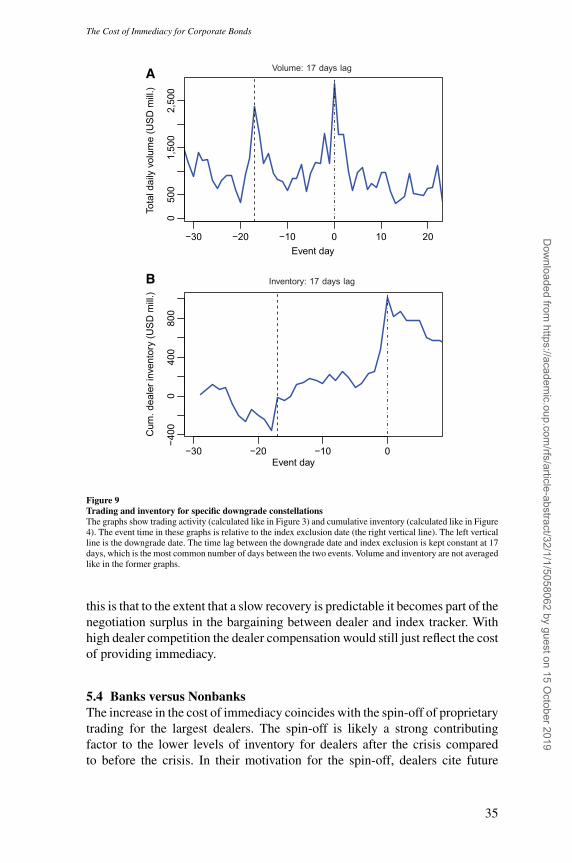
[17:21 17/12/2018 RFS-OP-REVF180082.tex] Page: 35 1–41
The Cost of Immediacy for Corporate Bonds
Volume: 17 days lag
Event day
To
tal d
aily
vo
lum
e (
US
D m
ill.)
05
00
1,5
00
2,5
00
−30 −20 −10 0 10 20
Inventory: 17 days lag
Event day
Cu
m.
de
ale
r in
ven
tory
(U
SD
mill
.)
−4
00
040
08
00
−30 −20 −10 0
A
B
Figure 9Trading and inventory for specific downgrade constellationsThe graphs show trading activity (calculated like in Figure 3) and cumulative inventory (calculated like in Figure4). The event time in these graphs is relative to the index exclusion date (the right vertical line). The left verticalline is the downgrade date. The time lag between the downgrade date and index exclusion is kept constant at 17days, which is the most common number of days between the two events. Volume and inventory are not averagedlike in the former graphs.
this is that to the extent that a slow recovery is predictable it becomes part of thenegotiation surplus in the bargaining between dealer and index tracker. Withhigh dealer competition the dealer compensation would still just reflect the costof providing immediacy.
5.4 Banks versus NonbanksThe increase in the cost of immediacy coincides with the spin-off of proprietarytrading for the largest dealers. The spin-off is likely a strong contributingfactor to the lower levels of inventory for dealers after the crisis comparedto before the crisis. In their motivation for the spin-off, dealers cite future
35
Dow
nloaded from https://academ
ic.oup.com/rfs/article-abstract/32/1/1/5058062 by guest on 15 O
ctober 2019

[17:2117/12/2018
RF
S-O
P-R
EV
F180082.tex]
Page:36
1–41
The
Review
ofFinancialStudies
/v32
n1
2019
Table 14Accounting for information
Event window: (0,t] 1 2 3 4 5 10 20 30
q*Post-crisis 1.429 2.202∗ 4.201∗∗ 5.590∗∗∗ 5.373∗∗∗ 3.643∗∗ 5.998∗∗ 7.558∗∗(1.329) (1.204) (1.781) (2.065) (1.832) (1.516) (2.699) (2.882)
q*Crisis 3.092∗∗ 3.829∗∗ 4.656∗∗ 6.276∗∗ 7.859∗∗∗ 6.699∗∗∗ 9.756∗∗∗ 9.471∗∗(1.313) (1.576) (1.997) (2.602) (2.830) (2.156) (3.015) (4.014)
q*Precrisis 0.112 0.118 0.110 0.264 0.248 0.255 0.00839 0.345(0.145) (0.168) (0.204) (0.222) (0.266) (0.351) (0.280) (0.437)
Recent downgrd −74.92∗∗∗ −94.36∗∗∗ −115.9∗∗∗ −105.0∗∗ −105.9∗∗ −79.72 30.72 87.61(23.22) (33.39) (39.05) (40.93) (42.09) (56.61) (60.18) (85.75)
Stk ret (excl.) −872.9∗∗ −1,048∗∗ −1,166∗∗ −1,103∗ −1,117∗∗ −1,700∗∗∗ −2,443∗∗∗ −1,257(350.5) (420.4) (478.6) (581.0) (550.9) (605.4) (882.6) (1,282)
MF change (pct) −298.3 −132.7 −391.3 −180.2 −27.45 398.3 −1,029∗ −1,447∗(257.7) (355.9) (396.8) (402.6) (545.8) (640.9) (565.4) (749.4)
Ins. change (pct) −183.5 −349.0 −72.76 89.27 241.0 −577.5 22.63 −1,110∗∗∗(272.5) (246.0) (435.9) (444.8) (620.1) (365.0) (520.9) (385.8)
% idx excluded 11.14∗∗ 28.43∗∗∗ 23.96∗∗ 17.04 25.59∗∗ 50.86∗∗ 46.51∗∗∗ 50.74(5.383) (10.38) (9.704) (10.55) (12.24) (19.68) (14.80) (32.05)
Log issue size −43.64∗∗∗ −43.96 −37.87 −18.25 −54.20 −78.84∗∗ −39.43 −31.14(16.00) (27.00) (36.05) (36.95) (42.49) (38.56) (25.93) (50.66)
Dealer lev. gwth −94.61 −248.2 −283.1 22.30 −80.62 −205.2 −124.1 −123.2(189.6) (284.2) (341.1) (436.9) (457.5) (405.3) (458.1) (520.1)
VIX 6.287 0.460 1.886 5.342 4.281 −5.037 8.493 15.80(4.623) (6.175) (7.557) (8.902) (8.876) (7.371) (8.684) (10.63)
TED spread 2.922∗∗ 4.752∗∗∗ 4.304∗∗∗ 4.192∗∗∗ 5.192∗∗∗ 2.859∗ 3.300 2.791(1.110) (0.868) (1.292) (1.560) (1.747) (1.645) (2.045) (2.555)
Observations 2,805 2,783 2,732 2,681 2,667 2,553 2,674 2,466Adjusted R-squared 0.376 0.409 0.420 0.424 0.447 0.355 0.566 0.549Dealer FEs Yes Yes Yes Yes Yes Yes Yes YesRating*Period FEs Yes Yes Yes Yes Yes Yes Yes Yes
This table presents regression coefficients for a series of regressions. The dependent variable is the bond- and dealer-specific abnormal return over the period from the exclusionday 0 to day t after exclusion. Variables are defined in Table 7. The regressions include (interacted) period/industry/rating and dealer fixed effects. The periods are 2002Q3–2007Q2(precrisis), 2007Q3–2009Q4 (crisis), and 2010Q1–2013Q4 (post-crisis). We consider two industry categories (financial vs. nonfinancial) and six rating categories (AAA–AA, A, BBB,BB, B, and CCC–C). Robust standard errors are clustered at the bond issuer and event date level. Robust standard errors are in parentheses. *** p<.01; ** p<.05; and * p<.1.
36
Dow
nloaded from https://academ
ic.oup.com/rfs/article-abstract/32/1/1/5058062 by guest on 15 O
ctober 2019

[17:21 17/12/2018 RFS-OP-REVF180082.tex] Page: 37 1–41
The Cost of Immediacy for Corporate Bonds
Table 15Bank versus nonbank reaction
A. Market share for banks (versus nonbanks)
Downgrade Maturity
Buy share Inv share Buy share Inv share
Post-crisis 0.696 0.874 0.663 0.640(0.016) (0.035) (0.017) (0.038)
Crisis 0.779 0.844 0.552 0.759(0.017) (0.030) (0.048) (0.160)
Precrisis 0.760 0.906 0.769 0.825(0.013) (0.025) (0.024) (0.047)
t-test (pre vs. post) 3.02∗∗∗ 0.75 3.61∗∗∗ 3.05∗∗∗
B. Diff-in-diff. of bank versus nonbank elasticity estimate
Window: (0,t] 1 3 5 10 20 30
q*Post-crisis*Bank 0.872*** 1.247*** 1.848*** 1.444*** 2.673*** 2.566***(0.317) (0.437) (0.641) (0.539) (0.688) (0.711)
q*Precrisis*Bank -0.142 -0.531* -0.294 -0.562** -0.0419 -0.162(0.191) (0.272) (0.336) (0.277) (0.283) (0.426)
Controls and lower-level interactions included
Observations 15,443 14,714 14,371 13,851 13,153 12,685Adj. R-squared 0.222 0.266 0.300 0.246 0.377 0.344Dealer FEs Yes Yes Yes Yes Yes YesRating*Period FEs Yes Yes Yes Yes Yes Yest-test (Diff-in-diff) 13.47∗∗∗ 24.89∗∗∗ 13.87∗∗∗ 14.40∗∗∗ 19.71∗∗∗ 12.48∗∗∗Panel A shows the market share fraction of the event buying volume handled by banks. The buy share is themarket share of the buying volume handled over event day -2 to 0. Inv share is the share of the total inventorybuildup held by banks over event day -2 to 0. Note that the later measure is not bounded between 0 and 1 becauseinventory buildup could be negative. All numbers are average across events for downgrade exclusions and maturityexclusions. The t-test is for no difference in estimates between precrisis and post-crisis. Panel B reports tripleinteractions of the form q∗Period ∗Bank, where Period is one of two subperiods: 2002Q3–2007Q2 (precrisis)and 2010Q1–2013Q4 (post-crisis). The triple interactions, including the one involving 2007Q3–2009Q4 (notreported to save space), are from regressions that are otherwise identical to those estimated in Table 12. A t-testfor the difference in the post-crisis interaction and the precrisis interaction is reported at the bottom of the table.Robust standard errors are in parentheses. *** p<.01; ** p<.05; and * p<.1.
regulation prohibiting proprietary trading, that is, the Volcker rule, as well asother regulations.
To test this potential channel, we follow Bao, O’Hara, and Zhou (2018) andclassify dealers as either banks or nonbanks. The Volcker rule was not actuallyimplemented during our sample period but the regulation was expected to beapplicable only to bank dealers. A differential increase in the cost of immediacybetween banks and nonbanks from before to after the crisis could thus suggestthat anticipation of tighter banking regulation was a contributing factor.
Table 15, panel A, shows the market share for banks versus nonbanks at theevents. Market share for banks is the fraction of the buying volume handled bybank dealers over day -2 to 0. Panel A also shows the share of the inventorybuildup over the same days for banks versus nonbanks. Inventory share is theinventory buildup for banks divided by the total inventory buildup for all dealers,hence, if either banks or nonbanks are net sellers at the event the inventory sharewill not be bounded by 0 and 1, although it is in most cases. The table shows thatthe market share for banks have decreased after the crisis, they handle less of
37
Dow
nloaded from https://academ
ic.oup.com/rfs/article-abstract/32/1/1/5058062 by guest on 15 O
ctober 2019

[17:21 17/12/2018 RFS-OP-REVF180082.tex] Page: 38 1–41
The Review of Financial Studies / v 32 n 1 2019
the overall activity and they account for less of the total inventory buildup. Thisis consistent with Duffie (2012), who argue that banning proprietary tradingwould allow for nonbanks to take over part of the market making. The inventoryshare decrease at the downgrade event for banks is fairly small. This couldbe a contributing factor explaining why the cost of immediacy has increasedmore for downgrades compared to maturity exclusions. For downgrade events,nonbanks have not yet taken over the supply of immediacy.
As an additional test, we augment the main regression with some tripleinteractions to capture banks’ change in trading behavior. The specificationthat we adopt is given by
P =β1q∗Post −crisis∗Bank+β2q∗Post −crisis
+β3q∗Crisis∗Bank+β4q∗Crisis
+β5Q∗Pre−crisis∗Bank+β6q∗Pre−crisis
+f ixed eff ects+controls+ε
(6)
The coefficients β1,β3, and β5 in Equation (6) measure the difference inelasticity between banks and nonbanks after, during, and before the crisis,respectively. A positive coefficient indicates that banks have a higher elasticitythan nonbanks. We are interested in assessing whether β1 is larger than β5, thatis whether the extent to which banks’ supply function is more elastic relativeto nonbanks has increased after the crisis.
For brevity, Table 15, panel B, shows only the triple interaction terms ofinterest. As the t-test at the bottom of the table shows, the difference in thedifference (β1 −β5) from before to after the crisis is positive and significant.This shows that the elasticity increases significantly more for banks comparedto nonbanks from before to after the crisis. This finding complements those ofBao, O’Hara, and Zhou (2018) and Bessembinder et al. (2018), who show aneffect at the implementation date of the Volcker rule. Our finding suggests thatfor the cost of immediacy there is also an earlier anticipation effect.17
6. Conclusion
The cost of immediacy for corporate bonds has significantly increased after the2008 crisis. We show that the supply of immediacy has become more elasticwith respect to its price and that dealers have become more reluctant to holdrisky bonds on inventory for longer periods of time. This post-crisis change inpricing and dealer behavior is most pronounced for banks, consistent with bankdealers closing down proprietary trading and operating with lower inventories.Furthermore, these findings are consistent with Duffie’s (2012) prediction thatthe post-crisis regulatory regime would impede market making.
17 Bao, O’Hara, and Zhou (2018) did not find a large anticipation effect, but their study was focused on fire salesin connection to the downgrade date. As shown in Section 5.3, that event may not be as focused on immediacyprovision as the event used in this study.
38
Dow
nloaded from https://academ
ic.oup.com/rfs/article-abstract/32/1/1/5058062 by guest on 15 O
ctober 2019
[17:21 17/12/2018 RFS-OP-REVF180082.tex] Page: 39 1–41
The Cost of Immediacy for Corporate Bonds
Whether or not the post-crisis regulation and less risky dealer inventories canbe considered a success depends on which segments of the economy will beaffected by future shocks. By encouraging traditional market makers to take onless risk than before the crisis, a shock is less likely to originate in the bankingsector (Johnson 2012; Richardson 2012). However, the lower willingness touse balance sheet for market making might make it more difficult for dealers tomitigate the selling pressure originating from shocks to other segments of theeconomy.
References
Admanti, A., and P. Pfleiderer. 1991. Sunshine trading and financial market equilibrium. Review of FinancialStudies 4:443–81.
Adrian, T., E. Etula, and T. Muir. 2014. Financial intermediaries and the cross-section of asset returns. Journalof Finance 69:2557—-96.
Adrian, T., M. Fleming, O. Shachar, and E. Vogt. 2015. Has U.S. corporate bond market liquidity deteriorated?Liberty Street Economics, October 5. http://libertystreeteconomics.newyorkfed.org/.
Ambrose, B., K. Cai, and J. Helwege. 2012. Fallen angels and price pressure. Journal of Fixed Income 21:74–86.
Amihud, Y., and H. Mendelson. 1980. Dealership market: Market-making with inventory. Journal of FinancialEconomics 8:31–53.
An, Y., and Z. Zheng. 2017. Conflicted immediacy provision. Working Paper.
Anand, A., C. Jotikasthira, and K. Venkataraman. 2017. Do buy-side institutions supply liquidity in bond markets?Evidence from mutual funds. Working Paper.
Bao, J., M. O’Hara, and X. Zhou. 2018. The Volcker rule and market-making in times of stress. Journal ofFinancial Economics. Advance Access published June 15, 2018, 10.1016/j.jfineco.2018.06.001.
Barber, B., and J. Lyon. 1997. Detecting long-run abnormal stock returns: The empirical power and specificationof test statistics. Journal of Financial Economics 43:341–72.
Beneish, M., and R. Whaley. 1996. An anatomy of the S&P game: The effects of changing the rules. Journal ofFinance 51:1909–30.
Bessembinder, H., S. Jacobsen, W. Maxwell, and K. Venkataraman. 2018. Capital commitment and illiquidityin corporate bonds. Journal of Finance. Advance Access published May 14, 2018, 10.1111/jofi.12694.
Bessembinder, H., K. Kahle, W. Maxwell, and D. Xu. 2009. Measuring abnormal bond performance. Review ofFinancial Studies 22:4219–58.
Blume, M., and R. Edelen. 2004. S&P 500 indexers, tracking error, and liquidity. Journal of Portfolio Management30:37–46.
Cai, N., J. Helwege, and A. Warga. 2007. Underpricing in the corporate bond market. Review of Financial Studies20:2021–46.
Chacko, G., J. Jurek, and E. Stafford. 2008. The price of immediacy. Journal of Finance 63:1253–90.
Chen, H., G. Noronha, and V. Singal. 2004. The price response to S&P 500 index additions and deletions:Evidence of asymmetry and a new explanation. Journal of Finance 59:1901–30.
———. 2006. Index changes and losses to index fund investors. Financial Analyst Journal 62:31–47.
Chen, Z., A. Lookman, N. Schurhoff, and D. Seppi. 2014. Rating-based investment practices and bond marketsegmentation. Review of Asset Pricing Studies 4:162–205.
39
Dow
nloaded from https://academ
ic.oup.com/rfs/article-abstract/32/1/1/5058062 by guest on 15 O
ctober 2019

[17:21 17/12/2018 RFS-OP-REVF180082.tex] Page: 40 1–41
The Review of Financial Studies / v 32 n 1 2019
Choi, D., M. Getmansky, B. Henderson, and H. Tookes. 2010. Convertible bond arbitrageurs as suppliers ofcapital. Review of Financial Studies 23:2492–522.
Choi, J., and Y. Huh. 2017. Customer liquidity provision: Implications for corporate bond transaction costs.Working Paper.
Dick-Nielsen, J. 2009. Liquidity biases in TRACE. Journal of Fixed Income 19:43–55.
Dick-Nielsen, J., P. Feldhutter, and D. Lando, 2012, Corporate bond liquidity before and after the onset of thesubprime crisis. Journal of Financial Economics 103:471–92.
Duffie, D. 2012. Market making under the proposed Volcker rule. Working Paper.
Duffie, D., N. Garleanu, and L. Pedersen. 2007. Valuation in over-the-counter markets. Review of FinancialStudies 20:1865–900.
Easley, D., and M. O’Hara. 1987. Price, trade size, and information in securities markets. Journal of FinancialEconomics 19:69–90.
Ellul, A., C. Jotikasthira, and C. Lundblad. 2011. Regulatory pressure and fire sales in the corporate bond market.Journal of Financial Economics 101:596–620.
Garman, M. 1976. Market microstructure. Journal of Financial Economics 3:257–75.
Goldstein, I., H. Jiang, and D. Ng. 2017. Investor flows and fragility in corporate bond funds. Journal of FinancialEconomics 126:592–613.
Goldstein, M., and E. Hotchkiss. 2008. Dealer behavior and the trading of newly issued corporate bonds. WorkingPaper.
Greenwood, R. 2005. Short- and long-term demand curves for stocks: Theory and evidence on the dynamics ofarbitrage. Journal of Financial Economics 75:607–49.
Grier, P., and S. Katz. 1976. The differential effects of bond rating changes among industrial and public utilitybonds by maturity. Journal of Business 49:226–39.
Harris, L., and E. Gurel. 1986. Price and volume effects associated with changes in the S&P 500 list: Newevidence for the existence of price pressures. Journal of Finance 41:815–29.
Hendershott, T., and A. Menkveld. 2014. Price pressures. Journal of Financial Economics 114:405–23.
Ho, T., and H. Stoll. 1981. Optimal dealer pricing under transactions and return uncertainty. Journal of FinancialEconomics 9:47–73.
Johnson, S. 2012. Restrictions on proprietary trading and certain interests in and relationships with hedge fundsand private equity funds. Comment letter to the SEC.
Katz, S. 1974. The price and adjustment process of bonds to rating reclassifications: A test of bond marketefficiency. Journal of Finance 29:551–9.
Lagos, R., and G. Rocheteau. 2007. Search in asset markets: Market structure, liquidity, and welfare. AmericanEconomic Review 97:198–202.
Levine, M. 2016. ETFs and U5s. Bloomberg, November 4.https://www.bloomberg.com/view/articles/2016-11-04/etfs-and-u5s.
Lou, D., H. Yan, and J. Zhang. 2013. Anticipated and repeated shocks in liquid markets. Review of FinancialStudies 26:1891–912.
Lucas, R. 1976. Econometric policy evaluation: A critique. In Carnegie-Rochester Conference Series on PublicPolicy. Amsterdam: Elsevier.
Madhavan, A., and S. Smidt. 1993. An analysis of changes in specialist inventories and quotations. Journal ofFinance 48:1595–628.
Mase, B. 2007. The impact of changes in the FTSE 100 index, Financial Review 42:461–84.
40
Dow
nloaded from https://academ
ic.oup.com/rfs/article-abstract/32/1/1/5058062 by guest on 15 O
ctober 2019

[17:21 17/12/2018 RFS-OP-REVF180082.tex] Page: 41 1–41
The Cost of Immediacy for Corporate Bonds
Newman, Y., and M. Rierson. 2004. Illiquidity spillovers: Theory and evidence from European telecom bondissuance. Working Paper.
Norden, L., and M. Weber. 2004. Informational efficiency of credit default swap and stock markets: The impactof credit rating announcements. Journal of Banking & Finance 28:2813–43.
Pedersen, L. 2018. Sharpening the arithmetic of active management. Financial Analyst Journal 74:21–36.
Petajisto, A. 2011. The index premium and its hidden cost for index funds. Journal of Empirical Finance18:271–88.
Richardson, M. 2012. Why the Volcker rule is a useful tool for managing systemic risk. White Paper.
Rossi, M. 2014. Realized volatility, liquidity, and corporate yield spreads. Quarterly Journal of Finance4:10.1142/S2010139214500049. Published online.
Schultz, P. 2001. Corporate bond trading costs: A peek behind the curtain. Journal of Finance 56:677–98.
Schwab. 2009. Schwab bond funds prospectus. White Paper.
Shleifer, A. 1986. Do demand curves for stocks slope down? Journal of Finance 41:579–90.
Stoll, H. 1978. The supply of dealer services in securities markets. Journal of Finance 33:1133–51.
Trebbi, F., and K. Xiao. 2017. Regulation and market liquidity. Management Science. Advance Access publishedDecember 9, 2017, 10.1287/mnsc.2017.2876.
Vanguard. 2009. Vanguard bond index funds prospectus. White Paper.
41
Dow
nloaded from https://academ
ic.oup.com/rfs/article-abstract/32/1/1/5058062 by guest on 15 O
ctober 2019