the correlation between the penetration force of cutting ... · the correlation between the...

The Correlation between the Penetration Force of Cutting Fluid and

Machining Stability by

Zhe Wang

A Thesis

Submitted to the Faculty

of the

Worcester Polytechnic Institute

In partial fulfillment of the requirements for the

Degree of Master of Science

in

Manufacturing Engineering

May 2010

Approved:

________________________________

Professor Mustapha S. Fofana, Advisor

________________________________

Professor Richard D. Sisson, Director of Manufacturing and Material Engineering

i

Abstract

The purpose of this thesis is to investigate the correlation between the penetration

force of cutting fluids and machining stability. General studies are made to understand

the classification of cutting fluids based on their chemical compositions. It is summarized

why the proper selection of cutting fluid for different machining processes is important.

The role of cutting fluids in machining process is documented as well as other related

issues such as delivery methods, storage, recycling, disposal and failure modes. The

uniqueness of this thesis is that it constructs a new mathematical model that would help

to explain and quantify the influence of the penetration force of cutting fluid on

machining stability. The basic principles of milling process, especially for thin wall

machining are reviewed for building the mathematical model. The governing equations of

the mathematical model are derived and solved analytically. The derived solutions are

used to construct the stability charts. The results show that there is a direct correlation

between the machining stability and the changes of the penetration force of the cutting

fluid. It is shown that the machining stability region is narrowed as the penetration force

of the cutting fluid increases while other machining variables are assumed to be constant.

This narrowness of the stability region is more obvious at spindle speed over 6000 rpm.

ii

Acknowledgements

Firstly, I would like to thank my advisor and my friend Professor Fofana. He has

devoted a lot to guide me through this thesis and my past two years of study here at

Worcester Polytechnic Institute. Then I would like to thank my parents who always

support me with love through my life. And I would like to thank Hui Cheng for her love

and support and tolerance during the preparation of this thesis. Finally my sincere

appreciation is extended to committee members of the thesis - Professor Sisson and

Professor Rong for their valuable support and contribution.

iii

Table of Contents

Abstract ................................................................................................................................ i

Acknowledgements .............................................................................................................. ii

Table of Contents ............................................................................................................... iii

List of Figures .................................................................................................................... iv

List of Tables ...................................................................................................................... vi

Chapter 1. Machining and Cutting Fluids ........................................................................... 1

Chapter 2. Classification of Cutting Fluids ........................................................................ 4 2.1. General Classification ...................................................................................... 4 2.2. Classification of Oil-based Fluids .................................................................... 5 2.3. Classification of Chemical Fluids .................................................................... 5 2.4. Cutting Fluid Impacts on Machining Processes............................................... 6

Chapter 3. Roles of Cutting Fluids in Machining Processes .............................................. 8 3.1. General Concepts ............................................................................................. 8 3.2. Basic Functions of Cutting Fluids.................................................................. 10 3.3. Delivery Methods........................................................................................... 14 3.4. Other Related Issues of Cutting Fluid ............................................................ 20

Chapter 4. Performance Evaluation of Cutting Fluids ...................................................... 29 4.1. Previous Studies ............................................................................................. 29 4.2. Review on Milling Operations ....................................................................... 31 4.3. Thin Wall Machining ..................................................................................... 36

Chapter 5. Mathematical Modeling of Milling Chatter and Cutting Fluid ....................... 41 5.1. Establishment of the Mathematical Model .................................................... 41 5.2. The Influence of Cutting Fluid Force on Milling .......................................... 48 5.3. The Cutting Fluid Force in Machining .......................................................... 54 5.4. Linear Stability Analysis................................................................................ 60

Chapter 6. Results and Discussions .................................................................................. 68

Chapter 7. Conclusion ....................................................................................................... 71

References ......................................................................................................................... 72

iv

List of Figures

Figure 1: Classification of cutting fluids 4

Figure 2: Orthogonal cutting geometry 8

Figure 3: Orthogonal cutting deformation and friction zones 9

Figure 4: Coolant pump for Haas Mill Drill Center 17

Figure 5: Flexible coolant pipe with a nozzle 18

Figure 6: Programmable nozzle 19

Figure 7: Installment of the nozzles in Haas Mill Drill Center 20

Figure 8: Contaminants in coolant sump 22

Figure 9: Recycling mechanism in Haas VF-4SS 24

Figure 10: A schematic system for all-in-one solution of cutting fluid 26

Figure 11: (a) Conventional milling vs. (b) Climb milling 33

Figure 12: Cutting forces resolutions in (a) Conventional milling and (b) Climb milling 34

Figure 13: Tool wear on end mill 35

Figure 14: Measuring the cutting forces in milling 36

Figure 15: Applications of thin wall machining 37

Figure 16: Thin wall machining instants 38

Figure 17: (a) Thin wall part (b) Dedicated fixture for machining thin wall parts 38

Figure 18: Angular position of cutter engagement 43

Figure 19: Cutting without cutting fluid - Operation setups 45

Figure 20: Cutting without cutting fluid - Motion geometry 45

Figure 21: Cutting without cutting fluid - Force components 46

Figure 22: Cutting with cutting fluid - Operation setups 46

v

Figure 23: Cutting with cutting fluid - Motion geometry and dynamic model 47

Figure 24: Cutting with cutting fluid - Force components 47

Figure 25: Stability lobes - Cutting without cutting fluid [2 flutes, 3 flutes and 4 flutes] 67

Figure 26: Stability lobes - Cutting with varying penetration force of cutting fluid 67

Figure 27: Cutting force under different pressure of coolant 70

vi

List of Tables

Table 1: Pros and cons of each type of cutting fluid 14

Table 2: Conventional contaminant removal equipment 23

Table 3: List of failure modes 27

1

Chapter 1. Machining and Cutting Fluids

Cutting fluid, as a component of machining industry, has been introduced and

applied for over 100 years. It is believed that W. H. Northcott is probably the first man to

mention the improvement in productivity that can be achieved when cutting fluid is

applied in machining process. This observation is published in his book “A Treatise on

Lathes and Turning” in 1868 (see 2). In 1907, F. W. Taylor pointed out that by applying a

heavy water stream on the tool/workpiece interface, the cutting speed can be increased

significantly by 30%-40% (see 45).

Since then, the technology of cutting fluids has been developed rapidly. Mineral,

vegetable and animal oil have all been introduced, which played important role in

enhancing various aspects of machining properties, including corrosion protection,

antibacterial protection, lubricity, chemical stability and even emulsibility. However, due

to the increasing cost of petroleum products, manufacturers starts to look for some

substitutes for oil, which accelerates the development of water-based fluids with different

chemical compositions performing different machining tasks. This effort also stimulates

the use of synthetic or semi-synthetic water-based fluids that contain only little or even

no oil. Study shows that water-based cutting fluids are now used in 80%-90% of all

machining applications [1].

Cutting fluids play an important role in modern machining industry. They can

impact the improvement of the surface finish, tool life and productivity significantly. Due

to the importance of cutting fluids, significant issues have been raised in their application,

recycling and disposal. Proper selection and application can reduce manufacturing cost

2

and improve productivity. On the other hand, manufacturing failure and wastes can be

experienced by misuse of cutting fluids. And regarding to the environmental impacts and

health hazards by cutting fluids, recycling and disposal of cutting fluid are also of great

importance. Improper disposal actions can cause severe health and environmental

problems. Such actions can even lead the substantial penalty level against companies by

the government agencies [2].

Numerous studies have been conducted to either investigate the impacts of the

cutting fluid on machining process or set up evaluation criteria to assist proper selection

and application of the cutting fluid. The goal of this thesis is to review and evaluate

cutting fluid related issues such as classification, functions, penetration forces and their

impact on machining processes. And due to the complexity of cutting fluid and many

issues that come with the application of cutting fluid, the thesis focus on investigating the

correlation between the penetration force of cutting fluid and the machining stability. The

mathematical model representing milling operation is constructed. The governing

equations of the motion are solved analytically to establish a direct correlation between

the penetration force of cutting fluid and the regimes of milling stability. As a result,

machining stability charts are constructed and in each of the charts stable spindle speed

are identified in terms of the correlation between the penetration force of cutting fluid and

milling stability.

The thesis is organized into seven chapters. Chapter 1 introduces the history and

modern development of cutting fluids and the purpose and structure of the thesis. Chapter

2 studies the classification of cutting fluids and their impact on the machining processes.

Chapter 3 presents the role of cutting fluids in machining processes and other related

3

issues based on the literature and our own experience in working at WPI machine shop.

Chapter 4 contains the performance evaluation of cutting fluids by previous researchers

and reviews the classical milling processes. Chapter 5 describes the unique mathematical

model, its governing equations, and presents the stability charts. Chapter 6 contains the

results and discussions. In Chapter 7 we summarize the correlation between the

penetration force of cutting fluid and machining stability.

4

Chapter 2. Classification of Cutting Fluids

2.1. General Classification

At the very first part of studying cutting fluid, it is of great importance to know

what kinds of cutting fluid are currently available in the market. This will provide an

opportunity to understand the forms and composition of the cutting fluid. Cutting fluids

have been an integral part of machining industry for many years. Numerous kinds of

cutting fluids are available in today’s market. They range from oil-based cutting fluid to

water-based [3]. Figure 1 summarizes the classification of cutting fluids. All of these

types of fluids are widely used in a variety of machining operations. Among these fluids,

synthetic fluids and semi-synthetic fluids are most suitable at high speed machining.

Figure 1: Classification of cutting fluids

5

2.2. Classification of Oil-based Fluids

Oil-based fluids can be sub-categorized into two types: straight oils and soluble

oils. Straight oils which contain no water are 100% petroleum or mineral oils. Some may

have particular additives to enhance their properties. Additives such as sulfur, chlorine or

phosphorus can improve the wettability, lubrication and antiwelding properties of oils.

The advantages of the straight oils include excellent lubrication, good rust protection,

good sump life, easy maintenance and rancid resistant. The disadvantages include poor

heat dissipation, increased risk of fire and oily film on workpiece. The application of this

type of oil-based fluids is limited to low-speed and severe cutting operations.

Soluble oils which are also called emulsifiable oils or water-soluble oils are 60%-

90% petroleum or mineral oils mixed with emulsifiers and other additives. The oils are

mixed with water and the emulsifiers cause the oil to distribute in the water thereby

forming an “oil-in-water” emulsion [4]. The advantages of the soluble oils include good

lubrication, improved cooling capabilities and good rust protection. This type of soluble

oils can be used for light to heavy duty operations. The disadvantages are more

susceptible to rust problems, bacterial growth, tramp oil contamination and evaporation

losses. They may form precipitates on machine, misting and oily film on workpiece. And

all of this would impact maintenance cost.

2.3. Classification of Chemical Fluids

Chemical fluids can be sub-categorized into two types: synthetic fluids and

semisynthetic fluids. Synthetic fluids contain no petroleum or mineral oils. It is provided

as a concentrate and mixed with water before use. Synthetic fluids can be further

6

classified as simple, complex or emulsifiable synthetic fluids based on their components

[5]. The advantages of the synthetic fluids are excellent microbial control, resistance to

rancidity, nonflammable and good corrosion control. The superior cooling qualities of the

synthetic fluids and their easy separation from the workpiece and chips prolong tool life

and improve the quality of machining applications. The disadvantages are reduced

lubrication and may cause misting, emulsify tramp oil and form residues. This

contaminants have adverse effects on machining operations.

Semisynthetic fluids which are also called semi-chemical fluids are a hybrid of

soluble oils and synthetic fluids. Basically they contain small portion of mineral oils

ranging from 2%-30% [6]. The balance portion mainly contains emulsifier, additives,

agents and water. The advantages of semisynthetic fluids include good microbial control,

resistance to rancidity and nonflammable. They have good corrosion control, good

cooling and lubrication. This form of fluid can be easily separated from workpiece and

chips. The disadvantages are water hardness impacts stability and may cause misting,

foaming and allergy, emulsify tramp oil and form residues.

2.4. Cutting Fluid Impacts on Machining Processes

The proper selection the cutting fluid is very critical for enhancing machining

processes performances. Different types of cutting fluids can deliver various kinds of

impact on the machining processes. There are substantial evidences in the literature why

the inappropriate use of cutting fluid will reduce the quality of machining operations.

J.M. Vieira et al. [36] have concluded in their paper that for high speed machining

of AISI 1020 steel under the cutting condition: 100-220 m/min for cutting speed, 0.1-0.25

7

mm/tooth for feed rate and 1.0-2.5 mm for depth of cut, semi-synthetic fluids will deliver

the best cooling results. Their study also indicated that the best surface roughness was

achieved when dry machining. This gives us the potential assumption that the cutting

fluid could possibly affect the machining stability so as to degrade the machining quality.

Xavior et al. [37] also conducted an experiment among coconut oil, soluble oil and

straight oil for testing their impacts on the surface roughness and tool wear on AISI 304

stainless steel under the cutting condition: 38.95/61.35/97.38 m/min for cutting speed,

0.5/1.0/1.2 mm for depth of cut and 0.2/0.25/0.28 mm/rev for feed rate. Their results

indicated that coconut oil performs better than the other two in terms of tool wear and

surface roughness. Belluco et al. [38] performed a drilling test on austenitic stainless steel

under the cutting condition: 25 m/min for cutting speed, 0.1 mm/rev for feed rate and 33

mm for the total drilling depth using vegetable-based oil and mineral oil. They observed

that vegetable-based oil produced better results than the mineral reference oil, the best

performance being 177% tool life increase and 7% reduction in thrust force with respect

to the commercial mineral oil. The results reflected not only the machining performance

improvement but also potential advantages for environmental concerns.

As a result, it can be seen that for different machining operations and cutting

conditions, the proper selection of cutting fluid is of great importance to maintain the

machining stability and quality.

In the next chapter, the roles of cutting fluids will be documented. They include

the basic functions of cutting fluid, delivery methods, storage, recycling, disposal and

possible failure modes. Real machining cases are also examined briefly in terms of these

issues mentioned above.

8

Chapter 3. Roles of Cutting Fluids in Machining Processes

3.1. General Concepts

In the previous chapter, we generally reviewed the classification of cutting fluids

and evaluated on their impact on the machining processes. To understand cutting fluids, tt

is of great importance to study their roles in machining processes as well.

Typically, cutting fluids play various roles during machining processes. The roles

include four main aspects which are cooling, lubrication, corrosion protection and chip

removal. To understand the roles of cutting fluids in process machining, we review the

deformation and friction in the cutting process. For simplicity, cutting forces involved in

a cutting operation are always examined in terms of an orthogonal cutting geometry

shown in Figure 2.

Figure 2: Orthogonal cutting geometry

t2

t1

Cutting

Workpiece

Tool Shear

Angle φ

Chip

9

One parameter that is usually mentioned when talking about machining process is

the cutting ratio. It is the ratio of depth of cut to thickness of chip. If the depth of cut is

kept constant, as the shear angle increases, one can easily see that the thickness of the

chip will decrease accordingly. This in turn reduces the cutting force. Consequently, the

power required per unit volume of metal and the heat generated will be reduced as well.

Figure 3: Orthogonal cutting deformation and friction zones

Figure 3 shows that there are four principle deformation zones along the

tool/workpiece and tool/chip interfaces. The primary deformation zone is where the most

energy is consumed during deforming. If the shear angle increases, the volume of

primary deformation zone will likely be reduced.

The secondary deformation zone is where the built-up edge (BUE) forms. The

BUE is a wedge-shaped quantity of workpiece material melted to the tip of the tool. It is

usually even harder than the workpiece itself as a consequence of the strain hardening

characteristics of the workpiece material. If the BUE is relatively large, it can decrease

Cutting

Workpiece

Tool

Chip

1

2

3

4

1: Primary deformation zone (shearing,

strain hardening)

2: Secondary deformation zone (BUE)

3: Primary friction zone (tool/chip

interface)

10

the effective rake angle and constantly degrade the finish quality of the workpiece surface

by forming and breaking away. By selecting a proper cutting fluid, the BUE can be

controlled to some extent.

Sliding friction would be another source of power consumption in cutting process.

It occurs at both the tool/chip interface and the tool/workpiece interface. Tool/chip

friction can be more significant than tool/workpiece friction, which can be a cause of rake

wear of the tool. Tool/workpiece friction appears to be a cause of flank wear of the tool.

3.2. Basic Functions of Cutting Fluids

The basic functions of cutting fluids typically include the following four

considerations: cooling, lubrication, corrosion protection and chip removal which are

going to be discussed in detail below.

a) Cooling

It is known that the energy generated in metal cutting operation both through

deformation and sliding friction process appears to be thermal energy or heat. It is also

indicated that over 60% of the thermal energy is generated in primary deformation zone;

while the rest is generated in secondary deformation zone and sliding friction zones [7].

The only advantage of the heat generated in cutting process is that it could reduce a

limited amount of forces required for deformation of the workpiece. However this

advantage is too limited compared with its disadvantages. The high temperature can

usually shorten the tool life, cause an undesirable surface finish and bring down the cycle

time due to the reduction of cutting speed. Basically, a cutting fluid should at least

acquire two key abilities to dissipate heat in good time during cutting process. One is to

11

gain access to the sources of heat and the other is to have the thermal capability to bring

heat away.

It is still not quite clear about how a cutting fluid make penetration into the

deformation and sliding friction zones. Several mechanisms have been proposed to model

the penetration process. It is believed that more than one such mechanism take actions at

the same time. However it appears that cutting fluids do penetrate and thereby causing

heat dissipation.

And to remove the heat, the cutting fluid should have the following capabilities:

thermal conductivity, specific heat, heat of vaporization and wettability with metal

surfaces. Water-based fluids and dilute emulsions have a significant advantage over oil-

based fluids in terms of thermal properties since water has a higher thermal conductivity

than organic oil. It is widely recognized in high-speed machining that water-based fluids

are used effectively. Vaporization is an effective way to remove heat since a large

amount of thermal energy generated by deformation and friction will transform fluid

from liquid state to gas state. It is also of great importance that the cutting fluid is capable

to wet the surface of the workpiece, since it will determine the effective cooling area. For

this capability, it is good for the fluid to have a low surface tension so that it can spread

on more area rather than only forming beads.

To validate the heat dissipation mechanism, monitoring the tool life change could

be an effective way as we mentioned previously. Other experiments indicate that

increasing fluid penetration and applying high-pressure jets can enhance the cooling

capabilities as well.

12

b) Lubrication

It is believed that due to high pressure and relatively high temperature in most

cutting operations, liquid film cannot be sustained along tool/workpiece interface for all

the time. Thus the conditions in a typical cutting process are believed to approach

boundary lubrication. In boundary lubrication, additives in the cutting fluid react with

both the workpiece material and the tool material to form chemical products on the

interface. This process is thought to include two interrelated mechanisms. First, the

lubricant absorbs into the chip surface and restricts the adhesion of chip material to the

tool. Second, reactive components of the fluid combine chemically with the freshly

generated metal surface of the chip to produce a film of lower shear strength than that of

the chip material, thus reducing sliding friction, forces and temperature. Extreme pressure

additives are often used to fulfill this function. Effective boundary lubrication must

achieve the requirements, namely the quantity of fluid additive should be sufficient to

take effects; the reactive composites in the additive should be available at the interface;

the temperature should be high enough to catalyze the reaction but not too high to make

the compound decompose or melt; the sliding speed should be relatively slow to allow

enough time for reaction to occur. Therefore if high cutting speed is applied, the fluid

accessibility would be limited, time for surface reaction will be decreased and some

lower-melting-point compound cannot be used. Most commercial cutting fluids employ

compounds of chlorine or sulfur as extreme pressure additives.

13

c) Corrosion Protection

It is of great importance to protect the workpiece from corrosion damage. One

method used to control the corrosion is to add soda ash to the cutting fluid, which will

likely increase the alkalinity of the fluid and reduce the possibility of rust.

Mineral oils are found to be a great deterrent to rust, which is able to form a

physical film along tool/workpiece interface to prevent chemical reaction from occurring.

However, along with the increase of cutting speed and hardness of the material, the

straight mineral oil may lack the ability to wet the machining surface. Thus some polar

compound additives are added to form emulsifiable oils. These emulsifiable oils combine

the cooling properties of water and lubrication abilities of mineral oil. These fluids as

well as semi-synthetic fluids are alkaline in nature to prevent workpiece surface from

corrosion damage [7].

Another widely-used fluid is the synthetic cutting fluid, which is defined as a

water-extendible product free of oil. A combination of alkanolamine and sodium nitrite

inhibitor package is used in this type of fluid. Therefore, this fluid can deliver superb

properties in cooling, rust protection, hard-water compatibility and biological resistance

[8]. Some other alternatives are also tested based on the concerns of healthy and

environmental issues.

d) Chip Removal

The fourth major function of cutting fluid in machining process is to remove chips

from the cutting zone. And the fluid will also prevent the machined surface from being

scratched by chips. This action is especially useful when dealing with operations like

14

deep-hole drilling, in which the cutting fluid is used under pressure and is fed through the

cutting tool to force the chips out of the hole. Proper selection of cutting fluid is still

important to avoid excessive foam generation that will interrupt with the machining

process [8].

Table 1 summarizes the advantages and disadvantages of each type of cutting

fluid for these four basic functions based on a good (G)-moderate (M)-poor (P) criterion.

Table 1: Pros and cons of each type of cutting fluid

Cooling Lubrication Corrosion

Protection Chip Removal

Straight oils P G G M

Soluble oils M G M M

Synthetic

fluids G M G M

Semi-

synthetic

fluids

G G G M

3.3. Delivery Methods

There are several methods available for use to deliver cutting fluids on the cutting

area during process machining. Three major application strategies are commonly used.

They are manual application, flood application and mist application [9].

The first strategy is manual application. It is often used for some very light duties

like small jobs or for hobbyists. The cutting fluid will be applied directly through the

cutting zone by the operator. The advantage of this method could be inexpensive and

15

easy to apply. However, there are bunch of disadvantages including intermittent

application of fluid which we would like to avoid, poor chip removal capability and

limited access to cutting zone since the operator can only brush the cutting fluid on the

surface of the workpiece. Thus, the use of manual application of cutting fluid is very

limited nowadays.

The second strategy, which is the most common, is flood application. Compared

with manual application, it is much more advantageous in terms of continuity of flow,

efficiency of chip removal and accessibility to cutting zone. Instead of manual

application by operator, a pump will deliver the cutting fluid from storage system to some

in-machine piping system and finally penetrate to the cutting zone through a nozzle. Thus

the cost of this application would be higher than manual but always reasonable for

factory manufacturing. For different operations, various configurations and flow rates

will be applied for optimized performance. For example, for turning operation, the flow

rate could be 5 gallon per minute; but for screw machining, the flow rate could range

from 35 to 60 gallon per minute based on the intensity of work. Frequently, two nozzles

will be used in one operation: one is flooding the fluid on the workpiece surface and the

other would be used to remove the chips and auxiliary cooling. For the shape of the

nozzle, the round one would be capable for most common machining and some fan-

shaped nozzles will be used for wider cutters.

The third strategy is mist application, which is best suited for high speed cutting

while cutting area is small. It can be an alternative method when flood application is

impractical. The disadvantage of mist application is the possibility of inhalation of the

mist by the operators. Thus good ventilation system is required to avoid this damage

16

happening. Two types of mist generators are used: one is the aspirator type and the other

is direct-pressure type. Other special application methods including chilled cutting fluid

and highly pressurized bottled gas are also proved to be effective for some specific

occasions. However, the cost of these applications is a big constraint which limits their

use in machining industry.

Numerous experiment evaluations have pointed out that it depends on the specific

machining operation that what type of delivery methods should be chosen. Traditionally,

it is ideal for most metal cutting applications to apply high-pressure and high-volume

cutting fluids to force a stream directly into the tool/workpiece and tool/chip interface

[10]. However, it cannot be always true. In the next chapter, a specific operation - thin

wall machining will be focused on and some problems related to cutting fluids will be

discussed.

The infrastructure of the delivery system is also very important to know. The

delivery system connects the storage system and the workpiece. It delivers cutting fluids

through a pump, a piping system and nozzles. Cutting fluid can be delivered to workpiece

through flood or mist application. For a flood application, fluid is directed under pressure

to the workpiece interface in a manner that produces maximum results. Pressure,

direction and shape of the stream are critical for an optimized performance. For a mist

application, fluids are atomized and blown onto the workpiece in form of mist. The

pressure and direction of the stream are also crucial to the success of the application.

The pump is used to get coolant from a sump to the machine. It is always

mounted at the side of the machine for an individual storage system or integrated in the

17

central reservoir system. A motor is usually accompanied to actuate the pump to work.

Figure 4 shows a typical structure of the pump system of Haas Mill Drill Center that is

used at WPI Washburn Shop.

It is also very critical to acquire the specifications of the pump for machine tool. It

reflects the capability of the pump for delivering the cutting fluid to the cutting space.

This capability varies from pump to pump. Common pumps used with daily CNC

machines are always centrifugal ones. A centrifugal pump can consume 3-5 horsepower

and is capable to reach a maximum pressure to 200 psi (approximately 1380 kPa). This

pressure can be adjusted by turning the valves either on the pump or on the piping system.

Thus it can be recognized that the pressure force delivered to the cutting area can be very

large [10].

Figure 4: Coolant pump for Haas Mill Drill Center

18

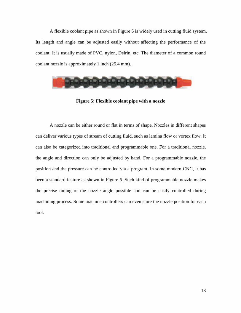
A flexible coolant pipe as shown in Figure 5 is widely used in cutting fluid system.

Its length and angle can be adjusted easily without affecting the performance of the

coolant. It is usually made of PVC, nylon, Delrin, etc. The diameter of a common round

coolant nozzle is approximately 1 inch (25.4 mm).

Figure 5: Flexible coolant pipe with a nozzle

A nozzle can be either round or flat in terms of shape. Nozzles in different shapes

can deliver various types of stream of cutting fluid, such as lamina flow or vortex flow. It

can also be categorized into traditional and programmable one. For a traditional nozzle,

the angle and direction can only be adjusted by hand. For a programmable nozzle, the

position and the pressure can be controlled via a program. In some modern CNC, it has

been a standard feature as shown in Figure 6. Such kind of programmable nozzle makes

the precise tuning of the nozzle angle possible and can be easily controlled during

machining process. Some machine controllers can even store the nozzle position for each

tool.

19

Figure 6: Programmable nozzle

It is also noticed that not only the angular position of the nozzles matters for the

performance of cutting fluids during the machining processes, but also the installed

position where altitude can be a factor that influences the performance. Figure 7 shows

the nozzles installed in Haas Mill Drill Center located at Worcester Polytechnic Institute,

Washburn Shops. From the picture, it can be observed that there is an extremely long

distance (approximately 10-15 inches) between the nozzle and cutting area. This could

make the delivery of the cutting fluid inconsistent and finally result in an unstable

machining.

20

Figure 7: Installment of the nozzles in Haas Mill Drill Center

3.4. Other Related Issues of Cutting Fluid

Besides the functional roles and delivery methods, there are some other related

issues about cutting fluid, including storage, recycling, disposal and failure modes. Each

of these issues can impact on the machining process. These impacts will not have been

studied in this thesis, but can be a good direction for the studies in the future.

21

a) Storage

The proper storage of cutting fluids is of great importance to prevent

contamination and deterioration. Some recommendations are given as follows for guiding

the proper storage of cutting fluids [11].

• Storing of fluid in clean seal-able drums clearly marked, protected from

frost or sunlight and preferably indoor;

• Have adequate ventilation and fire extinguishers in the storage area;

• Clean up spills with inert, mineral absorbent materials;

• Keep strong oxidizing agents out of the storage area;

• Do not use sawdust or oily cotton waste for spill control.

The storage sump for cutting fluids can be either placed with machine tool or

separately. For small work shop, the former is always applied due to its low cost and easy

setup. However, it is believed that for higher level applications, a central cutting fluid

storage system takes more advantages. Within such a system, the cutting fluid is stored in

one place and shared by several machine tools. The disadvantage is lack of flexibility of

the system. Since one system can often handle with one kind of cutting fluid at one time,

it may be difficult for dealing with various kinds of machining jobs.

Inappropriate storage of cutting fluids could result in some problems including

tramp oils, particle contaminants or bacteria and fungi generation. Figure 8 shows the

storage sump for Haas Mill Drill Center located at Worcester Polytechnic Institute,

Washburn Shops. It can be seen from the figure that if the coolant sump or tank is not

well sealed and exposed to the outside environment for a long time after use, the

22

problems mentioned above truly exist there and it is believed that it could lead to

potential machining problems.

Figure 8: Contaminants in coolant sump

b) Recycling

The quality of the cutting fluid will eventually reach a point that routine

maintenance is no longer effective. Then, it needs to be recycled or even disposed. To

recycle the fluid, the critical aspect is to recycle it at right time. The cutting fluid will

become not suitable for recycling if it degrades over the limit [12]. That is why

monitoring the quality and performance of cutting fluid is of great importance in fluid

management.

The conventional equipment for recycling is listed in Table 2.

23

Table 2: Conventional contaminant removal equipment

Equipment Contaminant Removed

Skimmers Tramp Oil

Coalescers Tramp Oil, Particulates

Flotation Tramp Oil, Particulates

Settling Tanks Particulates

Magnetic Separators Particulates

Hydrocyclones Particulates

Filtration Equipment Particulates

Centrifuges Tramp Oil, Particulates, Bacteria

Basically, the frequency for recycling the cutting fluid depends on the life

expectancy of the fluid itself. If the cutting fluid is required to be disposed after two or

three months, it should be treated monthly or if it is disposed only after two or three

weeks, it should be treated weekly. Typically, the contaminated fluid is sucked out of the

individual sump of each machine and placed in a batch-treatment recycling unit for

contaminant removal.

Some built-in recycling systems have already been deployed in modern CNC

machines. However, the impacts of these systems are limited due to the cost or other

issues. Figure 9 shows part of the recycling system in Haas Vertical Machining Center

VF-4SS located at Worcester Polytechnic Institute, Washburn Shops. The screw

mechanism in the picture is used to move out the chips away with the cutting fluids.

Some invisible filtration equipments are installed between this mechanism and the sump

at the bottom of the machine. However, by observing the sump after a long period

24

machining time, it is found that there are still contaminants such as tramp oils and micro

chips in the sump floating above the cutting fluid.

Figure 9: Recycling mechanism in Haas VF-4SS

c) Disposal

Even with the best recycling system, the cutting fluid will eventually deteriorate

and require being disposed. Due to extremely strict regulations by Federal and State

environment and health agencies, it is increasingly difficult to dispose the waste fluids. It

is required by regulations that the generator of the waste fluids is responsible for

determining whether the fluid is nonhazardous or hazardous. The cost for disposing the

waste fluid can range from 25 to 50 cents per gallon for nonhazardous waste up to

hundreds of dollars per drum for hazardous waste [4]. If the waste fluid is determined to

be hazardous, it must be disposed in EPA-certified treatment facilities while if it is

25

nonhazardous, it can be disposed in different ways such as being hauled to a treatment

facility, following permission from local wastewater treatment authorities or discharged

to a municipal sanitary sewer system.

The fluid should be disposed instead of recycling if any of the following happens:

• pH value is less than 8.0 while the normal range should be 8.5 to 9.4;

• Fluid concentration is less than 2.0% while the normal range should be 3.0%

to 12.0%;

• Appearance is dark grey to black while the normal range should be milky

white;

• Odor is strongly rancid or sour while the normal is a mild chemical smell.

Based on the current methods to recycle and dispose the cutting fluids and some

investigations in local manufacturing companies, it is concluded that it really costs a lot

of money to deal with the used cutting fluid, either to recycle or to dispose. According to

these concerns, we propose to establish a real-time monitoring system for the

performance of the cutting fluid in machining process. Such a system should be capable

to monitor the impact of cutting fluid on the machining process and make adjusts

according to the machining deviation automatically or give warnings to the machine

operator. Figure 10 shows a schematic structure of such a system. It is ideal to be a

closed-loop system which is able to self control with less human input. Also the storage

section of such a system should be more flexible than the current storage sump. Since it is

ideal for the storage drums to be sealed from the manufacturer to the machine tool all the

time, an interchangeable storage section could be constructed to make sure that the

26

cutting fluid will not be contaminated before reaching the cutting area. And the other

advantage of such a storage system could be that it can handle with different types of

cutting fluid easily and simultaneously by just switching on and off among several valves.

And more efficient filtration section should also be considered in such a system. Various

types of filtration equipment should be deployed for different sources of contaminants.

The purpose is to make sure that the cutting fluid is cleaned as much as possible before

returning to the storage section.

Figure 10: A schematic system for all-in-one solution of cutting fluid

d) Failure Modes

If the cutting fluid is not dealt with in a proper way in terms of one or more

aspects mentioned above, the machining process might fail in different ways. Table 3 is a

summary of failure modes and their causes and solutions [13].

27

Table 3: List of failure modes

Failure Mode Causes Solutions

Foaming

Concentration too high Adjust concentration

Machine cleaner in sump

Check pH

Allow machine to run, cleaner

should dissipate

Mechanical Check machinery and repair as

required

Soft water Sample water, treat it necessary

High tramp oil content

Skim off oil

Check hydraulic lines for leaks

and repair as required

Rusting

Concentration too low Adjust concentration

Poor mixing Add concentrate to water


Skim off oil



Poor Tool

Life

Concentration too low Adjust concentration

Wrong product being used Look up for right products

Large amounts of biocide added to

sump or system

Refer to operation manual for

right amounts


Skim off oil



Odor

Low concentration Adjust concentration

Low pH Check pH


Skim off oil



Contamination Sample and look for further

28

assistance from agents

Skin

Irritation

High concentration Adjust concentration

High pH Check pH


Skim off oil



Dirty shop clothes Use only clean cloths

Allergies Have operators checked for

allergies

Out-of-shop influences Check pH

Residue in

Machine

High concentration Adjust concentration


Skim off oil



Incorrect mixing Refer to operation manual

High misting operations Check ventilation system

Adjust coolant nozzles

Here are some common solutions for otential failure modes that could happen

when applying cutting fluids. Future studies may focus on building an intelligent expert

system with a knowledge library to help workshops to identify the cutting fluid problems

and provide proper solutions. Besides, more failure modes can be added to this

knowledge library, such as my following analysis.

In the next chapter, previous studies on evaluating the performance of cutting

fluids during machining processes will be reviewed. And since the specific milling

operation will be selected as the object we are going to model on for our own analysis,

the classical milling processes will also be reviewed, especially on thin wall machining.

29

Chapter 4. Performance Evaluation of Cutting Fluids

4.1. Previous Studies

Numerous preceding papers and works have been brought up to study the

performance evaluation of cutting fluids. Most of them focus on the impact brought by

cutting fluids on machining processes in terms of the type of the cutting fluid, the

delivery methods and different machining operations. Some of these studies are to try to

find some direct correlation between some aspects of cutting fluids and machining

performance. While some are to make efforts to establish some evaluation criteria to

assist the selection and application of cutting fluids in machining processes.

Axinte et al. [39] discussed effectiveness and resolution of five cutting tests

including turning, milling, drilling, tapping and VIPER grinding and their quality output

measures used in a multi-task procedure for evaluating the performance of cutting fluids

when machining aerospace materials. The resolution given by experimental data was

evaluated and a comparison of robustness in ranking the performance of cutting fluids

based on different output measures and cutting tests was presented.

Sales et al. [40] demonstrated some scratch test techniques which can be used to

provide a quick and cost effective evaluation of cutting fluids. Apparent coefficient of

friction and specific energy for the scratch steel samples under several lubrication

conditions provided a good indicator of cutting fluid performance which was followed by

evaluation of the surface finish and the cutting force of the ABNT NB 8640 steel with

emulsion and synthetic cutting fluids, at 5% of concentrations, and mineral oil in the

turning process. Comparative tests were carried out under dry and wet conditions. Results

30

showed that the linear scratch test was not efficient while the scratch test was efficient

tool in the classification of cutting fluids.

Axinte et al. [41] also described the results of a comprehensive evaluation

program for cutting fluid efficiency when machining the aerospace alloy Inconel 718.

The machining methods included milling, drilling, tapping and VIPER grinding, Results

from three cutting fluids including semi-synthetic fluids, synthetic fluids and emulsified

oils were. Cutting forces, torque and spindle power were acquired during machining.

Geometry accuracy surface texture and surface integrity of the workpiece were analyzed.

The experimental results demonstrated the difficulty for identifying the best cutting fluid,

especially when several different machining methods are employed on the machine tool.

It was unlikely that a single fluid could show the best performance on all machining trials.

Therefore, they established a multi-criteria model to assess the performance of cutting

fluids according to the time schedule for the customer. This methodology based on

various tests was proved to be able to evaluate the effectiveness of cutting fluid very

comprehensively.

Although amounts of studies have been performed previously, almost all of these

studies are based on the experimental results without mathematical modeling and analysis.

Very few of them focus on the dynamic impacts of cutting fluid on the machining

processes, especially the machining stability. This thesis attempts to establish a

correlation between the penetration force of cutting fluid and machining stability..

Based on the author’s own machining experience, this thesis is going to focus on

milling operations and thin wall. Thus in the following sections, general knowledge of

31

milling operations and thin wall machining is reviewed for the modeling analysis in the

next chapter.

4.2. Review on Milling Operations

Milling is the most widely used machining process the cutting tool carries out a

rotary motion and the workpiece is fed in a linear motion during milling. It is mostly used

for machining flat surfaces, slots and contoured features. Unlike turning, milling is

always a multi-point cutting process using face milling cutters or end mills. Generally

speaking, milling can be classified into two types based on different orientations of

spindle: one is horizontal milling and the other is vertical milling [14].

The characteristics of horizontal milling include:

• The cutting teeth are arranged on the surface of the cylindrical tool;

• There is a contact between the cylindrical surface of the cutter and the

machined surfaces;

• The machined surface is parallel to the cutter’s axis of rotation.

The characteristics of vertical milling include:

• The cutting edges are situated both on the face of the end mill and on its

cylindrical surface;

• There is a contact between the face of the milling cutter and the machined

surfaces;

• The machined surface is generated at right angle to the cutter axis of

rotation.

32

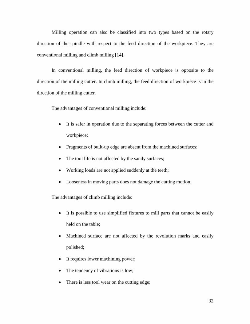
Milling operation can also be classified into two types based on the rotary

direction of the spindle with respect to the feed direction of the workpiece. They are

conventional milling and climb milling [14].

In conventional milling, the feed direction of workpiece is opposite to the

direction of the milling cutter. In climb milling, the feed direction of workpiece is in the

direction of the milling cutter.

The advantages of conventional milling include:

• It is safer in operation due to the separating forces between the cutter and

workpiece;

• Fragments of built-up edge are absent from the machined surfaces;

• The tool life is not affected by the sandy surfaces;

• Working loads are not applied suddenly at the teeth;

• Looseness in moving parts does not damage the cutting motion.

The advantages of climb milling include:

• It is possible to use simplified fixtures to mill parts that cannot be easily

held on the table;

• Machined surface are not affected by the revolution marks and easily

polished;

• It requires lower machining power;

• The tendency of vibrations is low;

• There is less tool wear on the cutting edge;

33

• It provides favorable cutting conditions that lead to better surface finish.

Generally speaking, climb milling is much preferred in today’s machining

practice. It can provide favorable cutting conditions such as lower cutting forces and less

tool wear which lead to better surface quality. Because the cutter is always tending to

climb on the workpiece, climb milling requires much stiffer equipment such as machine

tool and fixtures without looseness in the feeding mechanism. Along with the spreading

use of CNC machining center and other rigid machine tools, climb milling has been

applied over 99% out of all the milling processes in industry nowadays.

Figure 11 presents the difference between conventional milling and climb milling.

Figure 11: (a) Conventional milling vs. (b) Climb milling

No matter what type of milling it is, the cutting forces involved in milling

operation are tangential force perpendicular to the cutter radius and normal force along

the radius. The directions of the cutting forces are different depending on the type of

milling.

34

The resolution of forces in conventional milling and climb milling are shown in

Figure 12.

Figure 12: Cutting forces resolutions in (a) Conventional milling and (b) Climb milling

Cutting forces are widely recognized as an optimum performance estimator of

machining operations [15]. Large cutting forces are result of the extreme conditions at the

tool-workpiece interface. This interaction can be directly related to the tool wear and, in

the worst of the cases, lead to failure of the tool [16]. Consequently, tool wear and cutting

forces are related, although that relationship is different for each different wear

mechanism shown in Figure 13 (flank, crater, tool breakage).

35

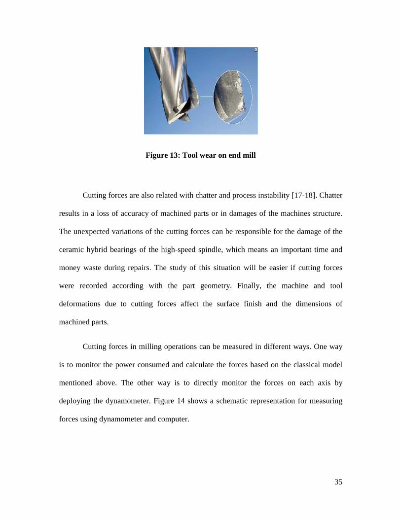
Figure 13: Tool wear on end mill

Cutting forces are also related with chatter and process instability [17-18]. Chatter

results in a loss of accuracy of machined parts or in damages of the machines structure.

The unexpected variations of the cutting forces can be responsible for the damage of the

ceramic hybrid bearings of the high-speed spindle, which means an important time and

money waste during repairs. The study of this situation will be easier if cutting forces

were recorded according with the part geometry. Finally, the machine and tool

deformations due to cutting forces affect the surface finish and the dimensions of

machined parts.

Cutting forces in milling operations can be measured in different ways. One way

is to monitor the power consumed and calculate the forces based on the classical model

mentioned above. The other way is to directly monitor the forces on each axis by

deploying the dynamometer. Figure 14 shows a schematic representation for measuring

forces using dynamometer and computer.

36

Figure 14: Measuring the cutting forces in milling

4.3. Thin Wall Machining

At present, thin walls are commonly applied in machining aeronautical and

aerospace components. Figure 15 shows some applications such as torpedoes and

airplane wings manufactured as thin wall machining. Thin wall parts contribute a lot to

decrease the weight of these products which have strict requirement for weight or

corrosion protection.

37

Figure 15: Applications of thin wall machining

Trial machining of thin wall parts have been done regularly at Worcester

Polytechnic Institute, Washburn Shops as lab contents for computer-aided manufacturing

class. During the labs, parts in different geometries shown in Figure 16 were machined at

various cutting conditions. Based on the machining experience and results, it was found

that machining in high speed would yield a good result while the machining stability

could not be guaranteed always. A fixture for machining thin wall parts was also applied

to improve the stiffness of the workpiece as to try to decrease the machining chatters as

shown in Figure 17.

38

Figure 16: Thin wall machining instants

Figure 17: (a) Thin wall part (b) Dedicated fixture for machining thin wall parts

39

Due to its very low stiffness, thin walls are difficult to machine. Wall deflection

or forced vibration and regenerative chatter can easily reduce the quality of thin wall

machining. These problems were studied by Smith and Dvorak [19]. They indicated that

one major limitation to the widespread use of high speed machining for the production of

thin components is the stability of the machining operation. As the wall becomes thinner,

it loses stiffness, and consequently, chatter will become more problematic. Such kind of

chatter during machining can result in poor surface quality, or even cutting through the

thin wall.

Some problems have been pointed out on thin wall machining from previous

research. The first problem is caused by the wall static deformation produced by the

cutting forces that generate an excess of uncut material. Wall deformation reduces the

tool immersion into the wall, and therefore, cutting forces decrease. As the operation

approaches the lower part of the wall, the stiffness becomes higher, and so the

deformation is smaller and the tool engagement is higher. It can result in an increase of

the cutting forces.

The second problem is caused by the machining dynamics. It is especially

important when the natural frequency of the wall is close to the teeth passing frequency.

It must be taken into account that the natural frequencies of a wall is continuously

decreasing during milling due to the progressive reduction of both the mass and stiffness

of the wall.

40

The third problem is caused by self-excited vibration, which is the cutting process

itself that generates oscillations. The origin of these oscillations, or chatter, is the

dynamic excitation produced by the wavy irregular part surface generated by precedent

tool tooth. This phenomenon is difficult to detect because the natural frequency of walls

changes during machining.

Lopez de Lacalle et al. [15] also indicated that these three types of problems may

happen at the same time. It can make it difficult to determine what the true origin of those

irregular marks that appears on a milled thin wall. However, besides these three problems

mentioned above, no one has considered about the impact of cutting fluid during

machining thin walls. Because of the application of high speed machining, it would

generate a relatively large amount of heat. And for soft materials like aluminum, the

chips are very adhesive to generate built-up edges and require to be flushed away

instantly during machining. Thus the use of cutting fluid is necessary in thin wall

machining. Therefore, the following analysis in the next chapter will focus on the impact

that is brought by the factor of cutting fluid on the machining stability.

41

Chapter 5. Mathematical Modeling of Milling Chatter and Cutting

Fluid

5.1. Establishment of the Mathematical Model

The single degree of freedom model describing the correlation between the

penetration force of cutting fluid and regenerative chatter milling is governed by the

delay differential equation:

𝑚𝑚�̈�𝑥(𝑡𝑡) + 𝑐𝑐�̇�𝑥(𝑡𝑡) + 𝑘𝑘𝑥𝑥(𝑡𝑡)

= ∆𝑓𝑓𝑥𝑥 �𝛼𝛼𝑗𝑗 (𝑡𝑡),∆ℎ𝑗𝑗𝑗𝑗 �𝑠𝑠𝑗𝑗𝑗𝑗 ,𝛼𝛼𝑗𝑗 (𝑡𝑡)� , 𝜇𝜇1� + ∆𝑔𝑔𝑐𝑐𝑥𝑥 �𝛼𝛼𝑗𝑗 (𝑡𝑡), �̇�𝑚�𝛼𝛼𝑗𝑗 (𝑡𝑡),𝜗𝜗�̇�𝑙(𝑡𝑡)�, 𝜇𝜇2�

(1)

where 𝑚𝑚 is the mass of the milling cutter, 𝑐𝑐 and 𝑘𝑘 are the viscous damping and stiffness

coefficients, respectively. The function ∆𝑓𝑓𝑥𝑥 �𝛼𝛼𝑗𝑗 (𝑡𝑡),∆ℎ𝑗𝑗𝑗𝑗 �𝑠𝑠𝑗𝑗𝑗𝑗 ,𝛼𝛼𝑗𝑗 (𝑡𝑡)� , 𝜇𝜇1� is the change in

cutting force along the 𝑥𝑥-direction and it is dependent upon the angular position 𝛼𝛼𝑗𝑗 (𝑡𝑡) of

the milling cutter of 𝑗𝑗-tooth at a specific time 𝑡𝑡, the variation of the feed ∆ℎ𝑗𝑗𝑗𝑗 �𝑠𝑠𝑗𝑗𝑗𝑗 ,𝛼𝛼𝑗𝑗 (𝑡𝑡)�

per 𝑗𝑗 -tooth generating 𝑠𝑠𝑗𝑗𝑘𝑘 -chip segments, and the parameter 𝜇𝜇1 . The parameter 𝜇𝜇1

represents the product of the width of cut 𝑤𝑤 and the ratio of the regenerative cutting force

𝑘𝑘1 and stiffness 𝑘𝑘 of cutter model. For 𝑗𝑗 ≤ 𝑗𝑗 = 1,2,3,⋯𝑛𝑛 and 𝑛𝑛 being a real integer, we

let 𝑧𝑧𝑗𝑗 to denote the total number of teeth in the cutter and 𝑧𝑧𝑗𝑗𝑐𝑐 to represent the number of 𝑗𝑗-

tooth of the milling cutter that are simultaneously in contact with the workpiece. The

regenerative time, denoted by 𝜏𝜏1 is defined as 𝜏𝜏1 = 2𝜋𝜋 �𝑧𝑧𝑗𝑗𝑐𝑐 Ω�⁄ where Ω is spindle speed

of the milling cutter in revolution per minute. Furthermore, let 𝛼𝛼𝑗𝑗 ,𝑒𝑒𝑛𝑛𝑡𝑡 (𝑡𝑡) and 𝛼𝛼𝑗𝑗 ,𝑒𝑒𝑥𝑥𝑒𝑒𝑡𝑡 (𝑡𝑡)

42

denote the entering angular position of the milling cutter of the 𝑗𝑗 -tooth at

ℎ𝑗𝑗𝑗𝑗 �𝑠𝑠𝑗𝑗𝑗𝑗 ,𝛼𝛼𝑗𝑗 (𝑡𝑡)�𝑚𝑚𝑒𝑒𝑛𝑛

and exiting angular position at chip thickness ℎ𝑗𝑗𝑗𝑗 �𝑠𝑠𝑗𝑗𝑗𝑗 ,𝛼𝛼𝑗𝑗 (𝑡𝑡)�𝑚𝑚𝑚𝑚𝑥𝑥

,

respectively. The feed per tooth ℎ𝑗𝑗𝑗𝑗 �𝑠𝑠𝑗𝑗𝑗𝑗 ,𝛼𝛼𝑗𝑗 (𝑡𝑡)� is described as ℎ𝑗𝑗𝑗𝑗 �𝑠𝑠𝑗𝑗𝑗𝑗 ,𝛼𝛼𝑗𝑗 (𝑡𝑡)� =

2𝜋𝜋𝜋𝜋 �𝑧𝑧𝑗𝑗𝑐𝑐 Ω�⁄ , where 𝜋𝜋 is the feedrate or the feed velocity of the machine tool table. And

then the 𝑗𝑗-tooth of the milling cutter removes material in the form of chips for 𝑧𝑧𝑗𝑗 =

𝑧𝑧𝑗𝑗𝑐𝑐 when the inequalities 𝛼𝛼𝑗𝑗 ,𝑒𝑒𝑛𝑛𝑡𝑡 (𝑡𝑡) ≤ 𝛼𝛼𝑗𝑗 (𝑡𝑡) ≤ 𝛼𝛼𝑗𝑗 ,𝑒𝑒𝑥𝑥𝑒𝑒𝑡𝑡 (𝑡𝑡) and ℎ𝑗𝑗𝑗𝑗 �𝑠𝑠𝑗𝑗𝑗𝑗 ,𝛼𝛼𝑗𝑗 (𝑡𝑡)�𝑚𝑚𝑒𝑒𝑛𝑛

≤

ℎ𝑗𝑗𝑗𝑗 �𝑠𝑠𝑗𝑗𝑗𝑗 ,𝛼𝛼𝑗𝑗 (𝑡𝑡)� ≤ ℎ𝑗𝑗𝑗𝑗 �𝑠𝑠𝑗𝑗𝑗𝑗 ,𝛼𝛼𝑗𝑗 (𝑡𝑡)�𝑚𝑚𝑚𝑚𝑥𝑥

hold. These inequalities, in particular, indicate that

machining is attainable, and that there is a continuous engagement between the 𝑗𝑗-tooth

and workpiece.

We make use of the fact that, the engagement may be discontinued at some

specific time in the interval 𝛼𝛼𝑗𝑗 ,𝑒𝑒𝑛𝑛𝑡𝑡 (𝑡𝑡) ≤ 𝛼𝛼𝑗𝑗 (𝑡𝑡) ≤ 𝛼𝛼𝑗𝑗 ,𝑒𝑒𝑥𝑥𝑒𝑒𝑡𝑡 (𝑡𝑡)so as to define the milling

engagement regime in the interval 𝛼𝛼𝑗𝑗 ,𝑒𝑒𝑛𝑛𝑡𝑡 (𝑡𝑡) ≤ 𝛼𝛼𝑗𝑗 (𝑡𝑡) ≤ 𝛼𝛼𝑗𝑗 ,𝑒𝑒𝑥𝑥𝑒𝑒𝑡𝑡 (𝑡𝑡), namely

𝜒𝜒𝑗𝑗𝑗𝑗 �𝛼𝛼𝑗𝑗 (𝑡𝑡), 𝑧𝑧𝑗𝑗𝑐𝑐 � ∶= 𝑠𝑠𝑒𝑒𝑔𝑔𝑛𝑛�𝛼𝛼𝑗𝑗 (𝑡𝑡), 𝑧𝑧𝑗𝑗𝑐𝑐 �

=

⎩⎪⎨

⎪⎧ 1, ℎ𝑗𝑗𝑗𝑗 �𝑠𝑠𝑗𝑗𝑗𝑗 ,𝛼𝛼𝑗𝑗 (𝑡𝑡)�

𝑚𝑚𝑒𝑒𝑛𝑛≤ ℎ𝑗𝑗𝑗𝑗 �𝑠𝑠𝑗𝑗𝑗𝑗 ,𝛼𝛼𝑗𝑗 (𝑡𝑡)� ≤ ℎ𝑗𝑗𝑗𝑗 �𝑠𝑠𝑗𝑗𝑗𝑗 ,𝛼𝛼𝑗𝑗 (𝑡𝑡)�

𝑚𝑚𝑚𝑚𝑥𝑥

0, ℎ𝑗𝑗𝑗𝑗 �𝑠𝑠𝑗𝑗𝑗𝑗 ,𝛼𝛼𝑗𝑗 (𝑡𝑡)� > ℎ𝑗𝑗𝑗𝑗 �𝑠𝑠𝑗𝑗𝑗𝑗 ,𝛼𝛼𝑗𝑗 (𝑡𝑡)�𝑚𝑚𝑚𝑚𝑥𝑥

> ℎ𝑗𝑗𝑗𝑗 �𝑠𝑠𝑗𝑗𝑗𝑗 ,𝛼𝛼𝑗𝑗 (𝑡𝑡)�𝑚𝑚𝑒𝑒𝑛𝑛

−1, ℎ𝑗𝑗𝑗𝑗 �𝑠𝑠𝑗𝑗𝑗𝑗 ,𝛼𝛼𝑗𝑗 (𝑡𝑡)�𝑚𝑚𝑒𝑒𝑛𝑛

< ℎ𝑗𝑗𝑗𝑗 �𝑠𝑠𝑗𝑗𝑗𝑗 ,𝛼𝛼𝑗𝑗 (𝑡𝑡)� < ℎ𝑗𝑗𝑗𝑗 �𝑠𝑠𝑗𝑗𝑗𝑗 ,𝛼𝛼𝑗𝑗 (𝑡𝑡)�𝑚𝑚𝑚𝑚𝑥𝑥

�

(2)

where the value of 𝜒𝜒𝑗𝑗𝑗𝑗 �𝛼𝛼𝑗𝑗 (𝑡𝑡), 𝑧𝑧𝑗𝑗𝑐𝑐 � = 1 indicates that 𝑗𝑗-tooth of the milling cutter are

cutting and for 𝜒𝜒𝑗𝑗𝑗𝑗 �𝛼𝛼𝑗𝑗 (𝑡𝑡), 𝑧𝑧𝑗𝑗𝑐𝑐 � = 0 , they are not cutting. In the interval 𝛼𝛼𝑗𝑗 ,𝑒𝑒𝑛𝑛𝑡𝑡 (𝑡𝑡) ≤

𝛼𝛼𝑗𝑗 (𝑡𝑡) ≤ 𝛼𝛼𝑗𝑗 ,𝑒𝑒𝑥𝑥𝑒𝑒𝑡𝑡 (𝑡𝑡) , interrupted or intermittent nonlinear milling forces may cause a

43

temporary disengagement between the 𝑗𝑗-teeth of the milling cutter and workpice, and the

value of 𝜒𝜒𝑗𝑗𝑗𝑗 �𝛼𝛼𝑗𝑗 (𝑡𝑡), 𝑧𝑧𝑗𝑗𝑐𝑐 � = −1 represents this aspect.

The angular position 𝛼𝛼𝑗𝑗 (𝑡𝑡) of the milling cutter of 𝑗𝑗-tooth is defined as 𝛼𝛼𝑗𝑗 (𝑡𝑡) =

Ω𝑡𝑡 + 𝛼𝛼𝑗𝑗 (𝑡𝑡0) where 𝛼𝛼𝑗𝑗 (𝑡𝑡0) is the equally spacing angle between adjacent milling teeth on

the cutter (see Figure 18) at some specific initial time 𝑡𝑡0.

Figure 18: Angular position of cutter engagement

We know that 𝛼𝛼𝑗𝑗 (𝑡𝑡0) = 2𝜋𝜋 𝑧𝑧𝑗𝑗⁄ and also 𝛼𝛼𝑗𝑗 (𝑡𝑡0) = 𝛼𝛼𝑗𝑗 (𝑡𝑡) 𝑧𝑧𝑗𝑗𝑐𝑐⁄ , and from these two

expressions yield

𝛼𝛼𝑗𝑗 (𝑡𝑡0) =2𝜋𝜋𝑧𝑧𝑗𝑗𝑐𝑐 + 𝑧𝑧𝑗𝑗𝛼𝛼𝑗𝑗 (𝑡𝑡)

𝑧𝑧𝑗𝑗 𝑧𝑧𝑗𝑗𝑐𝑐

(3a)

And hence we define angular position 𝛼𝛼𝑗𝑗 (𝑡𝑡) of the milling cutter of 𝑗𝑗-tooth as

44

𝛼𝛼𝑗𝑗 (𝑡𝑡) = Ω𝑡𝑡 + 𝛼𝛼𝑗𝑗 (𝑡𝑡0) =𝑧𝑧𝑗𝑗𝑐𝑐

𝑧𝑧𝑗𝑗𝑐𝑐 − 1�Ω𝑡𝑡 +

2𝜋𝜋𝑧𝑧𝑗𝑗𝑐𝑐𝑧𝑧𝑗𝑗

� (3b)

With the equally spacing angle 𝛼𝛼𝑗𝑗 (𝑡𝑡0), the magnitude of cutting force variation on

each 𝑗𝑗-tooth of the milling cutting will be the same, but for unequal spacing angle 𝛼𝛼𝑗𝑗 (𝑡𝑡0),

the impact of cutting force variation on each 𝑗𝑗-tooth changes. In such a situation we have

the angular position 𝛼𝛼𝑗𝑗 (𝑡𝑡) of the milling cutter of 𝑗𝑗-tooth as the form

𝛼𝛼𝑗𝑗 (𝑡𝑡) =𝑧𝑧𝑗𝑗𝑐𝑐

𝑠𝑠𝑒𝑒𝑔𝑔𝑛𝑛(𝑧𝑧𝑗𝑗𝑐𝑐 − 𝑧𝑧𝑗𝑗𝑐𝑐 ,𝑚𝑚𝑒𝑒𝑛𝑛 )− 1�Ω𝑡𝑡 +

2𝜋𝜋𝑧𝑧𝑗𝑗𝑐𝑐𝑧𝑧𝑗𝑗 𝑠𝑠𝑒𝑒𝑔𝑔𝑛𝑛(𝑧𝑧𝑗𝑗𝑐𝑐 − 𝑧𝑧𝑗𝑗𝑐𝑐 ,𝑚𝑚𝑒𝑒𝑛𝑛 )�

(4)

where 𝑧𝑧𝑗𝑗𝑐𝑐 ,𝑚𝑚𝑒𝑒𝑛𝑛 is the minimum number of 𝑗𝑗-tooth that are simultaneously in contact with

the workpiece at a particular time and maximum number is 𝑧𝑧𝑗𝑗𝑐𝑐 ,𝑚𝑚𝑚𝑚𝑥𝑥 = 𝑧𝑧𝑗𝑗𝑐𝑐 ,𝑚𝑚𝑒𝑒𝑛𝑛 +

𝑠𝑠𝑒𝑒𝑔𝑔𝑛𝑛(𝑧𝑧𝑗𝑗𝑐𝑐 − 𝑧𝑧𝑗𝑗𝑐𝑐 ,𝑚𝑚𝑒𝑒𝑛𝑛 ). The contact length of arc of the 𝑗𝑗-tooth in the interval 𝛼𝛼𝑗𝑗 ,𝑒𝑒𝑛𝑛𝑡𝑡 (𝑡𝑡) ≤

𝛼𝛼𝑗𝑗 (𝑡𝑡) ≤ 𝛼𝛼𝑗𝑗 ,𝑒𝑒𝑥𝑥𝑒𝑒𝑡𝑡 (𝑡𝑡) is given by 𝑙𝑙 = 𝛼𝛼𝑗𝑗 (𝑡𝑡)𝐷𝐷 2⁄ where 𝐷𝐷 is the diameter of the milling cutter.

The influence of the cutting fluid on cutting force variation has been one of the most

difficult influences to define and quantify. It is difficult to evaluate the influence from

knowledge of general practices of applying coolants into machining operations without

taking into considerations of the cutting fluid properties, velocities, forces and mass flow

rates. Attempt is made below to establish relations for cutting fluid influence.

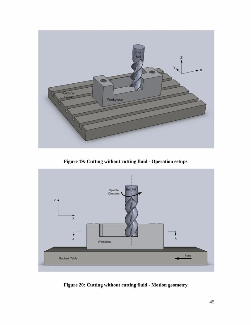
Before the mathematical analysis, the model that is studied is presented as follow.

Figure 19, Figure 20 and Figure 21 show the case that cutting without cutting fluid or we

say dry machining which include the operation setups, motion geometry and force

resolutions. Figure 22, Figure 23 and Figure 24 indicate the case that cutting fluid

impacts on the milling operation as compared with the first case.

45

Figure 19: Cutting without cutting fluid - Operation setups

Figure 20: Cutting without cutting fluid - Motion geometry

46

Figure 21: Cutting without cutting fluid - Force components

Figure 22: Cutting with cutting fluid - Operation setups

47

Figure 23: Cutting with cutting fluid - Motion geometry and dynamic model

Figure 24: Cutting with cutting fluid - Force components

48

5.2. The Influence of Cutting Fluid Force on Milling

Determination of the force variation ∆𝑔𝑔𝑐𝑐𝑥𝑥 = ∆𝑔𝑔𝑐𝑐𝑥𝑥 �𝛼𝛼𝑗𝑗 (𝑡𝑡), �̇�𝑚�𝛼𝛼𝑗𝑗 (𝑡𝑡),𝜗𝜗�̇�𝑙(𝑡𝑡)�, 𝜇𝜇2� of

the cutting fluid requires information about the mass flow rate �̇�𝑚�𝛼𝛼𝑗𝑗 (𝑡𝑡),𝜗𝜗�̇�𝑙(𝑡𝑡)� of the

cutting fluid into the interval 𝛼𝛼𝑗𝑗 ,𝑒𝑒𝑛𝑛𝑡𝑡 (𝑡𝑡) ≤ 𝛼𝛼𝑗𝑗 (𝑡𝑡) ≤ 𝛼𝛼𝑗𝑗 ,𝑒𝑒𝑥𝑥𝑒𝑒𝑡𝑡 (𝑡𝑡) of chip

thickness ℎ𝑗𝑗𝑗𝑗 �𝑠𝑠𝑗𝑗𝑗𝑗 ,𝛼𝛼𝑗𝑗 (𝑡𝑡)�𝑚𝑚𝑒𝑒𝑛𝑛

≤ ℎ𝑗𝑗𝑗𝑗 �𝑠𝑠𝑗𝑗𝑗𝑗 ,𝛼𝛼𝑗𝑗 (𝑡𝑡)� ≤ ℎ𝑗𝑗𝑗𝑗 �𝑠𝑠𝑗𝑗𝑗𝑗 ,𝛼𝛼𝑗𝑗 (𝑡𝑡)�𝑚𝑚𝑚𝑚𝑥𝑥

, namely

�̇�𝑚 �𝛼𝛼𝑗𝑗 (𝑡𝑡),𝜗𝜗�̇�𝑙(𝑡𝑡)�

= � �ℑ �𝛼𝛼𝑗𝑗 (𝑡𝑡),𝜗𝜗�̇�𝑙(𝑡𝑡)� + Θ111 �𝛼𝛼𝑗𝑗 (𝑡𝑡),𝜗𝜗�̇�𝑙(𝑡𝑡)�𝛼𝛼𝑗𝑗 ,𝑒𝑒𝑥𝑥𝑒𝑒𝑡𝑡 (𝑡𝑡)

𝛼𝛼𝑗𝑗 ,𝑒𝑒𝑛𝑛𝑡𝑡 (𝑡𝑡)

−Θ222 �𝛼𝛼𝑗𝑗 (𝑡𝑡),𝜗𝜗�̇�𝑙(𝑡𝑡)��𝑑𝑑𝛼𝛼𝑗𝑗 (𝑡𝑡)

(5)

where ℑ �𝛼𝛼𝑗𝑗 (𝑡𝑡),𝜗𝜗�̇�𝑙(𝑡𝑡)� is the mass flow rate that is carried by the milling cutter as it

rotates, Θ111 �𝛼𝛼𝑗𝑗 (𝑡𝑡),𝜗𝜗�̇�𝑙(𝑡𝑡)� represents the rate at which cutting fluid is flooded into the

milling process by ℓ-nozzle placed at some angular position with respect to the location

of cutting fluid streamline with coolant angular velocities 𝜗𝜗�̇�𝑙(𝑡𝑡) , ℓ = 1,2,3⋯𝑛𝑛 .

Θ222 �𝛼𝛼𝑗𝑗 (𝑡𝑡),𝜗𝜗�̇�𝑙(𝑡𝑡)� is the rate of cutting fluid mass that is outside the milling operation.

The parameter 𝜇𝜇2 denotes the ratio of the fluid force coefficient 𝑘𝑘�1 and stiffness 𝑘𝑘 of the

milling cutter. This is the force with which the cutting fluid penetrates the machining

operation. The variation of the chip thickness from ℎ𝑗𝑗𝑗𝑗 �𝑠𝑠𝑗𝑗𝑗𝑗 ,𝛼𝛼𝑗𝑗 (𝑡𝑡)� to ∆ℎ𝑗𝑗𝑗𝑗 �𝑠𝑠𝑗𝑗𝑗𝑗 ,𝛼𝛼𝑗𝑗 (𝑡𝑡)�

inside the interval 𝛼𝛼𝑗𝑗 ,𝑒𝑒𝑛𝑛𝑡𝑡 (𝑡𝑡) ≤ 𝛼𝛼𝑗𝑗 (𝑡𝑡) ≤ 𝛼𝛼𝑗𝑗 ,𝑒𝑒𝑥𝑥𝑒𝑒𝑡𝑡 (𝑡𝑡) influences the fluid penetration force

and mass flow rate �̇�𝑚 �𝛼𝛼𝑗𝑗 (𝑡𝑡),𝜗𝜗�̇�𝑙(𝑡𝑡)�. During machining, the cutting fluid moves ahead in

49

a given time instant at a point of least resistance from the chips. Coolants in recirculation

stages transport contaminants such as debris, chips and bacteria. Contaminations such as

tramps oil or chips would decrease fluid delivery force and mass flow rate because they

can clog the orifice diameter of the coolant nozzles. The contaminants will slow down the

rate of return of the cutting fluid from the nozzles into the interval 𝛼𝛼𝑗𝑗 ,𝑒𝑒𝑛𝑛𝑡𝑡 (𝑡𝑡) ≤ 𝛼𝛼𝑗𝑗 (𝑡𝑡) ≤

𝛼𝛼𝑗𝑗 ,𝑒𝑒𝑥𝑥𝑒𝑒𝑡𝑡 (𝑡𝑡) at depth of cut 𝑑𝑑 and chip thickness ℎ𝑗𝑗𝑗𝑗 �𝑠𝑠𝑗𝑗𝑗𝑗 ,𝛼𝛼𝑗𝑗 (𝑡𝑡)�𝑚𝑚𝑒𝑒𝑛𝑛

≤ ℎ𝑗𝑗𝑗𝑗 �𝑠𝑠𝑗𝑗𝑗𝑗 ,𝛼𝛼𝑗𝑗 (𝑡𝑡)� ≤

ℎ𝑗𝑗𝑗𝑗 �𝑠𝑠𝑗𝑗𝑗𝑗 ,𝛼𝛼𝑗𝑗 (𝑡𝑡)�𝑚𝑚𝑚𝑚𝑥𝑥

. The contaminants may present a hazard to the operator if not

properly collected and filtered. Insufficient and or intermittent coolant application in

milling operation, in particular, can lead to a situation where the cutting fluid may enter

the interval 𝛼𝛼𝑗𝑗 ,𝑒𝑒𝑛𝑛𝑡𝑡 (𝑡𝑡) ≤ 𝛼𝛼𝑗𝑗 (𝑡𝑡) ≤ 𝛼𝛼𝑗𝑗 ,𝑒𝑒𝑥𝑥𝑒𝑒𝑡𝑡 (𝑡𝑡) with stable spindle speeds but can be circulated

up to unstable spindle speeds before exiting the interval. One can think of this situation as

a change in the penetration force of the coolant and mass flow rate �̇�𝑚 �𝛼𝛼𝑗𝑗 (𝑡𝑡),𝜗𝜗�̇�𝑙(𝑡𝑡)� with

respect to the combined influence of the chip thickness variation ∆ℎ𝑗𝑗𝑗𝑗 �𝑠𝑠𝑗𝑗𝑗𝑗 ,𝛼𝛼𝑗𝑗 (𝑡𝑡)� and the

applied torques on the 𝑗𝑗-tooth of the milling cutter that arise from the gravitational,

damping and stiffness of the coolant and milling forces. Naturally one cannot, in general,

determine the quantities of Θ111 �𝛼𝛼𝑗𝑗 (𝑡𝑡),𝜗𝜗�̇�𝑙(𝑡𝑡)� and Θ222 �𝛼𝛼𝑗𝑗 (𝑡𝑡),𝜗𝜗�̇�𝑙(𝑡𝑡)� because of the

very long travel period of the cutting fluid before it reaches its intended storage systems.

Large coolant recirculation systems, coolant viscosities and degradations over time,

cutting tool geometry, coolant routes and application methods, machining conditions,

nozzle diameters and locations, and workpiece materials and shapes determine whether or

not there is sufficient mass of coolant to provide adequate cooling and chip clearing

capability. The considerations of high performance machining lead times are important in

50

designing a machining process and selecting an appropriate coolant. In this thesis work, a

great simplification of the force variation ∆𝑔𝑔𝑐𝑐𝑥𝑥 = ∆𝑔𝑔𝑐𝑐𝑥𝑥 �𝛼𝛼𝑗𝑗 (𝑡𝑡), �̇�𝑚�𝛼𝛼𝑗𝑗 (𝑡𝑡),𝜗𝜗�̇�𝑙(𝑡𝑡)�,𝜇𝜇2� of the

cutting fluid in the interval 𝛼𝛼𝑗𝑗 ,𝑒𝑒𝑛𝑛𝑡𝑡 (𝑡𝑡) ≤ 𝛼𝛼𝑗𝑗 (𝑡𝑡) ≤ 𝛼𝛼𝑗𝑗 ,𝑒𝑒𝑥𝑥𝑒𝑒𝑡𝑡 (𝑡𝑡) is thus the combined Fourier-

Taylor series representations

∆𝑔𝑔𝑐𝑐𝑥𝑥 �𝛼𝛼𝑗𝑗 (𝑡𝑡), �̇�𝑚�𝛼𝛼𝑗𝑗 (𝑡𝑡),𝜗𝜗�̇�𝑙(𝑡𝑡)�, 𝜇𝜇2�

= 𝑤𝑤�𝑘𝑘�1 �𝑥𝑥(𝑡𝑡) − 𝑥𝑥 �𝑡𝑡 − 𝜏𝜏𝑙𝑙�𝛼𝛼𝑗𝑗 (𝑡𝑡),𝜗𝜗�̇�𝑙(𝑡𝑡)��

+ 𝑤𝑤�𝑘𝑘�2 �𝑥𝑥(𝑡𝑡) − 𝑥𝑥 �𝑡𝑡 − 𝜏𝜏𝑙𝑙�𝛼𝛼𝑗𝑗 (𝑡𝑡),𝜗𝜗�̇�𝑙(𝑡𝑡)��2

+ 𝑤𝑤�𝑘𝑘�3 �𝑥𝑥(𝑡𝑡) − 𝑥𝑥 �𝑡𝑡 − 𝜏𝜏𝑙𝑙�𝛼𝛼𝑗𝑗 (𝑡𝑡),𝜗𝜗�̇�𝑙(𝑡𝑡)��3

+ ⋯𝑂𝑂 �𝑤𝑤�𝑘𝑘�5 �𝑥𝑥(𝑡𝑡) − 𝑥𝑥 �𝑡𝑡 − 𝜏𝜏𝑙𝑙�𝛼𝛼𝑗𝑗 (𝑡𝑡),𝜗𝜗�̇�𝑙(𝑡𝑡)��5�

(6a)

where the time-varying cutting fluid delay 𝜏𝜏𝑙𝑙�𝛼𝛼𝑗𝑗 (𝑡𝑡),𝜗𝜗�̇�𝑙(𝑡𝑡)� is the cosine and sine waves

defined by

⎩⎪⎨

⎪⎧ 𝜏𝜏𝑙𝑙�𝛼𝛼𝑗𝑗 (𝑡𝑡),𝜗𝜗�̇�𝑙(𝑡𝑡)� = 𝜏𝜏1 + 𝜀𝜀𝛾𝛾𝑙𝑙 �𝛼𝛼𝑗𝑗 (𝑡𝑡)� , 0 ≤ 𝜀𝜀 ≪ 1

𝛾𝛾 �𝛼𝛼𝑗𝑗 (𝑡𝑡)� = � 𝑚𝑚𝑚𝑚(1) cos𝜔𝜔𝑚𝑚 𝛼𝛼𝑗𝑗 (𝑡𝑡)

∞

𝑚𝑚=0

+ � 𝑚𝑚𝑚𝑚(2) sin𝜔𝜔𝑚𝑚 𝛼𝛼𝑗𝑗 (𝑡𝑡)

∞

𝑚𝑚=1

�

(6b)

and the Fourier constants 𝑚𝑚𝑚𝑚(0), 𝑚𝑚𝑚𝑚

(1)and 𝑚𝑚𝑚𝑚(2), namely

51

⎩⎪⎪⎪⎪⎪⎪⎪⎪⎨

⎪⎪⎪⎪⎪⎪⎪⎪⎧ 𝑚𝑚𝑚𝑚

(0) =1

Γ �𝛼𝛼𝑗𝑗 (𝑡𝑡),𝜗𝜗�̇�𝑙(𝑡𝑡)�∙

� �� 𝑚𝑚𝑚𝑚(1) cos𝜔𝜔𝑚𝑚 𝛼𝛼𝑗𝑗 (𝑡𝑡)

∞

𝑚𝑚=0


∞

𝑚𝑚=1

�𝑑𝑑𝛼𝛼𝑗𝑗 (𝑡𝑡)

Γ�𝛼𝛼𝑗𝑗 (𝑡𝑡),𝜗𝜗𝑙𝑙̇ (𝑡𝑡)�

0

𝑚𝑚𝑚𝑚(1) =

1



∞

𝑚𝑚=0


∞

𝑚𝑚=1

� cos𝜔𝜔𝑚𝑚 𝛼𝛼𝑗𝑗 (𝑡𝑡)𝑑𝑑𝑡𝑡


0

𝑚𝑚𝑚𝑚(2) =

1



∞

𝑚𝑚=0


∞

𝑚𝑚=1

� sin𝜔𝜔𝑚𝑚 𝛼𝛼𝑗𝑗 (𝑡𝑡)𝑑𝑑𝑡𝑡


0

�

(6c)

and 𝜔𝜔𝑚𝑚 are the amplitudes and frequencies of the cutting fluid delivered into the milling

operation. Using the fact that

𝑥𝑥(𝑡𝑡) − 𝑥𝑥 �𝑡𝑡 − �𝜏𝜏2 + 𝜀𝜀𝛾𝛾𝑙𝑙 �𝛼𝛼𝑗𝑗 (𝑡𝑡)�� ∶= 𝑥𝑥(𝑡𝑡) − 𝑥𝑥(𝑡𝑡 − 𝜏𝜏2)

+ 𝜀𝜀 � �̇�𝑥 �𝑡𝑡 + 𝛼𝛼𝑗𝑗 (𝑡𝑡)� 𝑑𝑑𝛼𝛼𝑗𝑗 (𝑡𝑡)𝑡𝑡−𝜏𝜏2

𝑡𝑡−�𝜏𝜏2+𝜀𝜀𝛾𝛾𝑙𝑙�𝛼𝛼𝑗𝑗 (𝑡𝑡)��

(6d)

we can write Equation (6a) as follows

52

∆𝑔𝑔𝑐𝑐𝑥𝑥 �𝛼𝛼𝑗𝑗 (𝑡𝑡), �̇�𝑚�𝛼𝛼𝑗𝑗 (𝑡𝑡),𝜗𝜗�̇�𝑙(𝑡𝑡)�, 𝜇𝜇2�

= −𝑤𝑤� �𝑘𝑘�1 �𝑥𝑥(𝑡𝑡) − 𝑥𝑥(𝑡𝑡 − 𝜏𝜏1) + 𝜀𝜀 � �̇�𝑥�𝑡𝑡 + 𝛼𝛼𝑗𝑗 (𝑡𝑡)�𝑑𝑑𝛼𝛼𝑗𝑗 (𝑡𝑡)𝑡𝑡−𝜏𝜏1

𝑡𝑡−�𝜏𝜏1+𝜀𝜀𝛾𝛾𝑙𝑙(𝛼𝛼𝑗𝑗 (𝑡𝑡))��

+ 𝑘𝑘�2 �𝑥𝑥(𝑡𝑡) − 𝑥𝑥(𝑡𝑡 − 𝜏𝜏1) + 𝜀𝜀 � �̇�𝑥�𝑡𝑡 + 𝛼𝛼𝑗𝑗 (𝑡𝑡)�𝑑𝑑𝛼𝛼𝑗𝑗 (𝑡𝑡)𝑡𝑡−𝜏𝜏1


2

+ 𝑘𝑘�3 �𝑥𝑥(𝑡𝑡) − 𝑥𝑥(𝑡𝑡 − 𝜏𝜏1) + 𝜀𝜀 � �̇�𝑥�𝑡𝑡 + 𝛼𝛼𝑗𝑗 (𝑡𝑡)�𝑑𝑑𝛼𝛼𝑗𝑗 (𝑡𝑡)𝑡𝑡−𝜏𝜏1


3

+ ⋯𝑂𝑂�𝑘𝑘�5 �𝑥𝑥(𝑡𝑡) − 𝑥𝑥(𝑡𝑡 − 𝜏𝜏1)

+ 𝜀𝜀 � �̇�𝑥�𝑡𝑡 + 𝛼𝛼𝑗𝑗 (𝑡𝑡)�𝑑𝑑𝛼𝛼𝑗𝑗 (𝑡𝑡)𝑡𝑡−𝜏𝜏1


5

��

(6e)

The time delay 𝜏𝜏2 corresponds to the nominal value of the mass of the fluid

delivered into the milling operation for ℎ𝑗𝑗𝑗𝑗 �𝑠𝑠𝑗𝑗𝑗𝑗 ,𝛼𝛼𝑗𝑗 (𝑡𝑡)�𝑚𝑚𝑒𝑒𝑛𝑛

≤ ℎ𝑗𝑗𝑗𝑗 �𝑠𝑠𝑗𝑗𝑗𝑗 ,𝛼𝛼𝑗𝑗 (𝑡𝑡)� ≤

ℎ𝑗𝑗𝑗𝑗 �𝑠𝑠𝑗𝑗𝑗𝑗 ,𝛼𝛼𝑗𝑗 (𝑡𝑡)�𝑚𝑚𝑚𝑚𝑥𝑥

and in the interval 𝛼𝛼𝑗𝑗 ,𝑒𝑒𝑛𝑛𝑡𝑡 (𝑡𝑡) ≤ 𝛼𝛼𝑗𝑗 (𝑡𝑡) ≤ 𝛼𝛼𝑗𝑗 ,𝑒𝑒𝑥𝑥𝑒𝑒𝑡𝑡 (𝑡𝑡). This time delay 𝜏𝜏2

is determined by the length of travel of the coolant and velocity it travels with as it

enters 𝛼𝛼𝑗𝑗 ,𝑒𝑒𝑛𝑛𝑡𝑡 (𝑡𝑡) ≤ 𝛼𝛼𝑗𝑗 (𝑡𝑡) ≤ 𝛼𝛼𝑗𝑗 ,𝑒𝑒𝑥𝑥𝑒𝑒𝑡𝑡 (𝑡𝑡). 𝑤𝑤 is the width in which the coolant is delivered

inside the interval 𝛼𝛼𝑗𝑗 ,𝑒𝑒𝑛𝑛𝑡𝑡 (𝑡𝑡) ≤ 𝛼𝛼𝑗𝑗 (𝑡𝑡) ≤ 𝛼𝛼𝑗𝑗 ,𝑒𝑒𝑥𝑥𝑒𝑒𝑡𝑡 (𝑡𝑡) . The parameters 𝑘𝑘�1, 𝑘𝑘�2,⋯𝑘𝑘�𝑗𝑗 , 𝑗𝑗 =

1,2,3,⋯ represent the coefficients of the nonlinearity after Taylor expansion of

∆𝑔𝑔𝑐𝑐𝑥𝑥 �𝛼𝛼𝑗𝑗 (𝑡𝑡), �̇�𝑚�𝛼𝛼𝑗𝑗 (𝑡𝑡),𝜗𝜗�̇�𝑙(𝑡𝑡)�,𝜇𝜇2� at some nominal value of the mass flow rate of the

cutting fluid in the interval 𝛼𝛼𝑗𝑗 ,𝑒𝑒𝑛𝑛𝑡𝑡 (𝑡𝑡) ≤ 𝛼𝛼𝑗𝑗 (𝑡𝑡) ≤ 𝛼𝛼𝑗𝑗 ,𝑒𝑒𝑥𝑥𝑒𝑒𝑡𝑡 (𝑡𝑡) . The time-varying delay

53

parameter 𝛾𝛾𝑙𝑙 �𝛼𝛼𝑗𝑗 (𝑡𝑡)� and the nonlinearity will continue to fluctuate no matter how small

or large the induced cutting force variation ∆𝑓𝑓𝑥𝑥 �𝛼𝛼𝑗𝑗 (𝑡𝑡),∆ℎ𝑗𝑗𝑗𝑗 �𝑠𝑠𝑗𝑗𝑗𝑗 ,𝛼𝛼𝑗𝑗 (𝑡𝑡)� , 𝜇𝜇1� is. The

appearance of 𝛼𝛼𝑗𝑗 (𝑡𝑡) in the Fourier representation of the mass

variation ∆𝑔𝑔𝑐𝑐𝑥𝑥 �𝛼𝛼𝑗𝑗 (𝑡𝑡), �̇�𝑚�𝛼𝛼𝑗𝑗 (𝑡𝑡),𝜗𝜗�̇�𝑙(𝑡𝑡)�, 𝜇𝜇2� serves to explain the correlation between this

variation and that of the cutting force ∆𝑓𝑓𝑥𝑥 �𝛼𝛼𝑗𝑗 (𝑡𝑡),∆ℎ𝑗𝑗𝑗𝑗 �𝑠𝑠𝑗𝑗𝑗𝑗 ,𝛼𝛼𝑗𝑗 (𝑡𝑡)� , 𝜇𝜇1� in the

interval 𝛼𝛼𝑗𝑗 ,𝑒𝑒𝑛𝑛𝑡𝑡 (𝑡𝑡) ≤ 𝛼𝛼𝑗𝑗 (𝑡𝑡) ≤ 𝛼𝛼𝑗𝑗 ,𝑒𝑒𝑥𝑥𝑒𝑒𝑡𝑡 (𝑡𝑡) . The angular position of the nozzles, which is

freely adjusted to different positions between the machine-tool spindle and work piece

and oil or chip contaminants, may transport high gravitational and damping torques as the

cutting fluid enters in the interval 𝛼𝛼𝑗𝑗 ,𝑒𝑒𝑛𝑛𝑡𝑡 (𝑡𝑡) ≤ 𝛼𝛼𝑗𝑗 (𝑡𝑡) ≤ 𝛼𝛼𝑗𝑗 ,𝑒𝑒𝑥𝑥𝑒𝑒𝑡𝑡 (𝑡𝑡) . The Fourier

representation of ∆𝑔𝑔𝑐𝑐𝑥𝑥 �𝛼𝛼𝑗𝑗 (𝑡𝑡), �̇�𝑚�𝛼𝛼𝑗𝑗 (𝑡𝑡),𝜗𝜗�̇�𝑙(𝑡𝑡)�,𝜇𝜇2� in Equation (6) thus gives us better

estimates of the amplitudes and frequencies of the cutting fluid delivered into j-teeth of

the milling cutter at 𝛼𝛼𝑗𝑗 ,𝑒𝑒𝑛𝑛𝑡𝑡 (𝑡𝑡) ≤ 𝛼𝛼𝑗𝑗 (𝑡𝑡) ≤ 𝛼𝛼𝑗𝑗 ,𝑒𝑒𝑥𝑥𝑒𝑒𝑡𝑡 (𝑡𝑡) and of depth of cut d and chip

thickness ℎ𝑗𝑗𝑗𝑗 �𝑠𝑠𝑗𝑗𝑗𝑗 ,𝛼𝛼𝑗𝑗 (𝑡𝑡)�𝑚𝑚𝑒𝑒𝑛𝑛

≤ ℎ𝑗𝑗𝑗𝑗 �𝑠𝑠𝑗𝑗𝑗𝑗 ,𝛼𝛼𝑗𝑗 (𝑡𝑡)� ≤ ℎ𝑗𝑗𝑗𝑗 �𝑠𝑠𝑗𝑗𝑗𝑗 ,𝛼𝛼𝑗𝑗 (𝑡𝑡)�𝑚𝑚𝑚𝑚𝑥𝑥

. The Fourier

representation has a sufficient structure to evaluate relationships and phenomena for long

term variations of both ∆𝑓𝑓𝑥𝑥 �𝛼𝛼𝑗𝑗 (𝑡𝑡),∆ℎ𝑗𝑗𝑗𝑗 �𝑠𝑠𝑗𝑗𝑗𝑗 ,𝛼𝛼𝑗𝑗 (𝑡𝑡)� , 𝜇𝜇1�

and ∆𝑔𝑔𝑐𝑐𝑥𝑥 �𝛼𝛼𝑗𝑗 (𝑡𝑡), �̇�𝑚�𝛼𝛼𝑗𝑗 (𝑡𝑡),𝜗𝜗�̇�𝑙(𝑡𝑡)�, 𝜇𝜇2�. The amplitudes, frequencies and stability regimes

of the milling operation of various mass of the cutting fluid in the interval 𝛼𝛼𝑗𝑗 ,𝑒𝑒𝑛𝑛𝑡𝑡 (𝑡𝑡) ≤

𝛼𝛼𝑗𝑗 (𝑡𝑡) ≤ 𝛼𝛼𝑗𝑗 ,𝑒𝑒𝑥𝑥𝑒𝑒𝑡𝑡 (𝑡𝑡) can be calculated in a more direct way. The threshold of the attainable

variations of ∆𝑓𝑓𝑥𝑥 �𝛼𝛼𝑗𝑗 (𝑡𝑡),∆ℎ𝑗𝑗𝑗𝑗 �𝑠𝑠𝑗𝑗𝑗𝑗 ,𝛼𝛼𝑗𝑗 (𝑡𝑡)� , 𝜇𝜇1� and ∆𝑔𝑔𝑐𝑐𝑥𝑥 �𝛼𝛼𝑗𝑗 (𝑡𝑡), �̇�𝑚�𝛼𝛼𝑗𝑗 (𝑡𝑡),𝜗𝜗�̇�𝑙(𝑡𝑡)�, 𝜇𝜇2� is

represented by the finite nature of the nonlinearities and sizes of the time varying delays.

Generalization of this representation to other forms of cutting fluids and machining

54

operations is attainable as well. The small parameter 𝜀𝜀 has values of the form 0 ≤ 𝜀𝜀 ≪ 1,

and it is scaling factor of the nonlinearities in ∆𝑓𝑓𝑥𝑥 �𝛼𝛼𝑗𝑗 (𝑡𝑡),∆ℎ𝑗𝑗𝑗𝑗 �𝑠𝑠𝑗𝑗𝑗𝑗 ,𝛼𝛼𝑗𝑗 (𝑡𝑡)� , 𝜇𝜇1�

and ∆𝑔𝑔𝑐𝑐𝑥𝑥 �𝛼𝛼𝑗𝑗 (𝑡𝑡), �̇�𝑚�𝛼𝛼𝑗𝑗 (𝑡𝑡),𝜗𝜗�̇�𝑙(𝑡𝑡)�, 𝜇𝜇2�. The next section is concerned with the aspects of

deriving the cutting force variation ∆𝑓𝑓𝑥𝑥 �𝛼𝛼𝑗𝑗 (𝑡𝑡),∆ℎ𝑗𝑗𝑗𝑗 �𝑠𝑠𝑗𝑗𝑗𝑗 ,𝛼𝛼𝑗𝑗 (𝑡𝑡)� , 𝜇𝜇1� in terms of the chip

thickness variation ∆ℎ𝑗𝑗𝑗𝑗 �𝑠𝑠𝑗𝑗𝑗𝑗 ,𝛼𝛼𝑗𝑗 (𝑡𝑡)�.

5.3. The Cutting Fluid Force in Machining

The cutting force variation along the 𝑥𝑥-direction as seen in Figure 8 is given by

∆𝑓𝑓𝑥𝑥 �𝛼𝛼𝑗𝑗 (𝑡𝑡),∆ℎ𝑗𝑗𝑗𝑗 �𝑠𝑠𝑗𝑗𝑗𝑗 ,𝛼𝛼𝑗𝑗 (𝑡𝑡)� , 𝜇𝜇1�

= −𝑤𝑤�𝜒𝜒𝑗𝑗𝑗𝑗 �𝛼𝛼𝑗𝑗 (𝑡𝑡), 𝑧𝑧𝑗𝑗𝑐𝑐 � × 𝑓𝑓𝑗𝑗𝑥𝑥 �∆ℎ𝑗𝑗𝑗𝑗 �𝑠𝑠𝑗𝑗𝑗𝑗 ,𝛼𝛼𝑗𝑗 (𝑡𝑡),𝑑𝑑�𝑘𝑘𝑗𝑗𝑥𝑥 �𝛼𝛼𝑗𝑗 (𝑡𝑡), 𝜇𝜇1��

𝑧𝑧𝑗𝑗

𝑗𝑗=1

(7)

where 𝑓𝑓𝑗𝑗𝑥𝑥 �∆ℎ𝑗𝑗𝑗𝑗 �𝑠𝑠𝑗𝑗𝑗𝑗 ,𝛼𝛼𝑗𝑗 (𝑡𝑡),𝑑𝑑�� is the cutting force variation that is dependent only on the

feed ∆ℎ𝑗𝑗𝑗𝑗 �𝑠𝑠𝑗𝑗𝑗𝑗 ,𝛼𝛼𝑗𝑗 (𝑡𝑡)� per tooth and depth of cut 𝑑𝑑 . 𝑘𝑘𝑗𝑗𝑥𝑥 �𝛼𝛼𝑗𝑗 (𝑡𝑡), 𝜇𝜇1� is the cutting force

coefficient per unit area and is equivalent to 𝐹𝐹𝑗𝑗𝑥𝑥 �𝛼𝛼𝑗𝑗 (𝑡𝑡), 𝜇𝜇1�. By the geometry of the

cutter-workpiece interaction in Figure 15 we have the expressions for ∆ℎ𝑗𝑗𝑗𝑗 �𝑠𝑠𝑗𝑗𝑗𝑗 ,𝛼𝛼𝑗𝑗 (𝑡𝑡)�

and 𝐹𝐹𝑗𝑗𝑥𝑥 �𝛼𝛼𝑗𝑗 (𝑡𝑡), 𝜇𝜇1�, as follows

ℎ𝑗𝑗𝑗𝑗 �𝑠𝑠𝑗𝑗𝑗𝑗 ,𝛼𝛼𝑗𝑗 (𝑡𝑡)� = 𝑠𝑠𝑗𝑗𝑗𝑗 sin𝛼𝛼𝑗𝑗 (𝑡𝑡) (8a)

with

55

∆ℎ𝑗𝑗𝑗𝑗 �𝑠𝑠𝑗𝑗𝑗𝑗 ,𝛼𝛼𝑗𝑗 (𝑡𝑡)� = ℎ𝑗𝑗𝑗𝑗 �𝑠𝑠𝑗𝑗𝑗𝑗 ,𝛼𝛼𝑗𝑗 (𝑡𝑡)�𝑐𝑐ℎ𝑚𝑚𝑡𝑡𝑡𝑡𝑒𝑒𝜋𝜋

− ℎ𝑗𝑗𝑗𝑗 �𝑠𝑠𝑗𝑗𝑗𝑗 ,𝛼𝛼𝑗𝑗 (𝑡𝑡)�𝑧𝑧𝑒𝑒𝜋𝜋𝑧𝑧𝑐𝑐 ℎ𝑚𝑚𝑡𝑡𝑡𝑡𝑒𝑒𝜋𝜋

= �𝑠𝑠𝑗𝑗0 + 𝑥𝑥(𝑡𝑡) − 𝑥𝑥 �𝑡𝑡 − 𝜏𝜏𝑗𝑗 (𝑡𝑡)�� sin𝛼𝛼𝑗𝑗 (𝑡𝑡) − 𝑠𝑠𝑗𝑗0 sin𝛼𝛼𝑗𝑗 (𝑡𝑡)

= �𝑥𝑥(𝑡𝑡) − 𝑥𝑥 �𝑡𝑡 − 𝜏𝜏𝑗𝑗 (𝑡𝑡)�� sin𝛼𝛼𝑗𝑗 (𝑡𝑡)

(8b)

and the cutting force

𝐹𝐹𝑗𝑗𝑥𝑥 �𝛼𝛼𝑗𝑗 (𝑡𝑡), 𝜇𝜇1� = 𝐹𝐹𝑗𝑗𝑡𝑡 cos𝛼𝛼𝑗𝑗 (𝑡𝑡) + 𝐹𝐹𝑗𝑗𝜋𝜋 sin𝛼𝛼𝑗𝑗 (𝑡𝑡) (8c)

with the relationship 𝐹𝐹𝑗𝑗𝜋𝜋 = 𝐹𝐹𝑗𝑗𝑡𝑡 tan𝛽𝛽 yield

𝐹𝐹𝑗𝑗𝑥𝑥 �𝛼𝛼𝑗𝑗 (𝑡𝑡), 𝜇𝜇1� = 𝐹𝐹𝑗𝑗𝑡𝑡 cos𝛼𝛼𝑗𝑗 (𝑡𝑡) + 𝐹𝐹𝑗𝑗𝑡𝑡 tan𝛽𝛽 sin𝛼𝛼𝑗𝑗 (𝑡𝑡) = 𝐹𝐹𝑗𝑗𝑡𝑡 �cos𝛼𝛼𝑗𝑗 (𝑡𝑡) + tan𝛽𝛽 sin𝛼𝛼𝑗𝑗 (𝑡𝑡)�

= �1 + tan2 𝛽𝛽 𝐹𝐹𝑗𝑗𝑡𝑡 cos�𝛼𝛼𝑗𝑗 (𝑡𝑡) − 𝜗𝜗0�

(8d)

where

cos𝜗𝜗0 =1

�1 + tan2 𝛽𝛽, sin𝜗𝜗0 =

tan𝛽𝛽�1 + tan2 𝛽𝛽

(8e)

and this lead to the simplification of Equation (7) into the form

56


= −�1 + tan2 𝛽𝛽𝑤𝑤�𝜒𝜒𝑗𝑗𝑗𝑗 �𝛼𝛼𝑗𝑗 (𝑡𝑡), 𝑧𝑧𝑗𝑗𝑐𝑐 �

𝑧𝑧𝑗𝑗

𝑗𝑗=1

× 𝑓𝑓𝑗𝑗𝑥𝑥 �∆ℎ𝑗𝑗𝑗𝑗 �𝑠𝑠𝑗𝑗𝑗𝑗 ,𝛼𝛼𝑗𝑗 (𝑡𝑡),𝑑𝑑�𝑘𝑘𝑗𝑗𝑥𝑥 �𝛼𝛼𝑗𝑗 (𝑡𝑡),𝜇𝜇1� cos�𝛼𝛼𝑗𝑗 (𝑡𝑡) − 𝜗𝜗0� sin𝛼𝛼𝑗𝑗 (𝑡𝑡)�

(8f)

The minus sign −∆𝑓𝑓𝑥𝑥 of the cutting force variation of the 𝑗𝑗-tooth indicates that a

positive relative displacement of the cutter removes a feed ℎ𝑗𝑗𝑗𝑗 �𝑠𝑠𝑗𝑗𝑗𝑗 ,𝛼𝛼𝑗𝑗 (𝑡𝑡)� per tooth of

material and at depth of cut 𝑑𝑑. 𝑠𝑠𝑗𝑗0 is the segment at the steady state nominal feed per 𝑗𝑗-

tooth of the milling cutter. 𝑥𝑥(𝑡𝑡) is the state of the milling cutter and 𝑥𝑥(𝑡𝑡 − 𝜏𝜏(𝑡𝑡)) is the

earlier state 𝑥𝑥(𝑡𝑡 − 𝜏𝜏(𝑡𝑡)) at time 𝑡𝑡 − 𝜏𝜏𝑗𝑗 (𝑡𝑡) . It is known that cutting force 𝐹𝐹𝑗𝑗𝑡𝑡 =

𝐹𝐹𝑗𝑗𝑡𝑡 �𝑤𝑤, 𝜋𝜋,𝑑𝑑,ℎ𝑗𝑗𝑗𝑗 �𝑠𝑠𝑗𝑗𝑗𝑗 ,𝛼𝛼𝑗𝑗 (𝑡𝑡)�� is function of the cutting parameters, namely, the width of

cut 𝑤𝑤, feedrate 𝜋𝜋, depth of cut 𝑑𝑑 and feed per tooth ℎ𝑗𝑗𝑗𝑗 �𝑠𝑠𝑗𝑗𝑗𝑗 ,𝛼𝛼𝑗𝑗 (𝑡𝑡)�. For the depth of cut

variation, we define the corresponding cutting force coefficients 𝑘𝑘𝑗𝑗𝑥𝑥 �𝛼𝛼𝑗𝑗 (𝑡𝑡), 𝜇𝜇1� as follow

𝑘𝑘𝑗𝑗𝑥𝑥 �𝛼𝛼𝑗𝑗 (𝑡𝑡), 𝜇𝜇1� ∶= −�𝜕𝜕𝑗𝑗𝐹𝐹𝑗𝑗𝑡𝑡 �𝑤𝑤, 𝜋𝜋,𝑑𝑑,ℎ𝑗𝑗𝑗𝑗 �𝑠𝑠𝑗𝑗𝑗𝑗 ,𝛼𝛼𝑗𝑗 (𝑡𝑡)��

𝑗𝑗! 𝜕𝜕𝑑𝑑𝑗𝑗�

𝑑𝑑=𝑑𝑑0

= 𝑘𝑘1 + 𝑘𝑘2(𝑘𝑘1),𝑘𝑘3(𝑘𝑘1), +⋯𝑘𝑘𝑗𝑗+1(𝑘𝑘1), 𝑗𝑗 = 1,2,3,⋯

(9)

where 𝜕𝜕𝑗𝑗𝐹𝐹𝑗𝑗𝑡𝑡 (∙)

𝑗𝑗 !𝜕𝜕𝑑𝑑𝑗𝑗 are 𝑗𝑗-partial derivatives of 𝐹𝐹𝑗𝑗𝑡𝑡 �𝑤𝑤, 𝜋𝜋,𝑑𝑑,ℎ𝑗𝑗𝑗𝑗 �𝑠𝑠𝑗𝑗𝑗𝑗 ,𝛼𝛼𝑗𝑗 (𝑡𝑡)�� with respect to 𝑑𝑑 .

And 𝑘𝑘𝑗𝑗 are the respective cutting coefficients after the Taylor expansion of 𝐹𝐹𝑗𝑗𝑡𝑡 =

𝐹𝐹𝑗𝑗𝑡𝑡 �𝑤𝑤, 𝜋𝜋,𝑑𝑑,ℎ𝑗𝑗𝑗𝑗 �𝑠𝑠𝑗𝑗𝑗𝑗 ,𝛼𝛼𝑗𝑗 (𝑡𝑡)�� . Next we consider the Taylor expansion of

57

𝑓𝑓𝑗𝑗𝑥𝑥 �∆ℎ𝑗𝑗𝑗𝑗 �𝑠𝑠𝑗𝑗𝑗𝑗 ,𝛼𝛼𝑗𝑗 (𝑡𝑡)� ,𝑑𝑑� with respect to the feed ℎ𝑗𝑗𝑗𝑗 �𝑠𝑠𝑗𝑗𝑗𝑗 ,𝛼𝛼𝑗𝑗 (𝑡𝑡)� per tooth and compute

the Taylor coefficients at depth of cut 𝑑𝑑 = 𝑑𝑑0, thus we obtain

𝑓𝑓𝑗𝑗𝑥𝑥 �∆ℎ𝑗𝑗𝑗𝑗 �𝑠𝑠𝑗𝑗𝑗𝑗 ,𝛼𝛼𝑗𝑗 (𝑡𝑡)� ,𝑑𝑑�

= (1!)−1𝑓𝑓𝑗𝑗𝑥𝑥(1)(𝑑𝑑0)�𝑥𝑥(𝑡𝑡) − 𝑥𝑥(𝑡𝑡 − 𝜏𝜏𝑗𝑗 (𝑡𝑡)� sin𝛼𝛼𝑗𝑗 (𝑡𝑡)

+ (2!)−1𝑓𝑓𝑗𝑗𝑥𝑥(2)(𝑑𝑑0)��𝑥𝑥(𝑡𝑡) − 𝑥𝑥(𝑡𝑡 − 𝜏𝜏𝑗𝑗 (𝑡𝑡)� sin𝛼𝛼𝑗𝑗 (𝑡𝑡)�2

+ (3!)−1𝑓𝑓𝑗𝑗𝑥𝑥(3)(𝑑𝑑0)��𝑥𝑥(𝑡𝑡) − 𝑥𝑥(𝑡𝑡 − 𝜏𝜏𝑗𝑗 (𝑡𝑡)� sin𝛼𝛼𝑗𝑗 (𝑡𝑡)�3

+ ⋯𝑂𝑂 �𝑓𝑓𝑗𝑗𝑥𝑥(5)(𝑑𝑑0)��𝑥𝑥(𝑡𝑡) − 𝑥𝑥(𝑡𝑡 − 𝜏𝜏𝑗𝑗 (𝑡𝑡)� sin𝛼𝛼𝑗𝑗 (𝑡𝑡)�5�

(10a)

where 𝑓𝑓𝑗𝑗𝑥𝑥 �∆ℎ𝑗𝑗𝑗𝑗 �𝑠𝑠𝑗𝑗𝑗𝑗 ,𝛼𝛼𝑗𝑗 (𝑡𝑡)� ,𝑑𝑑� , 𝑗𝑗 = 1,2,⋯ are again the partial derivatives and

comparing this Equation (10a) with Equation (9), we have

𝑓𝑓𝑗𝑗𝑥𝑥 �∆ℎ𝑗𝑗𝑗𝑗 �𝑠𝑠𝑗𝑗𝑗𝑗 ,𝛼𝛼𝑗𝑗 (𝑡𝑡)� ,𝑑𝑑�

= 𝑘𝑘1�𝑥𝑥(𝑡𝑡) − 𝑥𝑥(𝑡𝑡 − 𝜏𝜏𝑗𝑗 (𝑡𝑡)� sin𝛼𝛼𝑗𝑗 (𝑡𝑡)

+ 𝑘𝑘2��𝑥𝑥(𝑡𝑡) − 𝑥𝑥(𝑡𝑡 − 𝜏𝜏𝑗𝑗 (𝑡𝑡)� sin𝛼𝛼𝑗𝑗 (𝑡𝑡)�2


+⋯𝑂𝑂 �𝑘𝑘5��𝑥𝑥(𝑡𝑡) − 𝑥𝑥(𝑡𝑡 − 𝜏𝜏𝑗𝑗 (𝑡𝑡)� sin𝛼𝛼𝑗𝑗 (𝑡𝑡)�5�

(10b)

Hence the substitution of Equations (9) and (10) into (8) gives

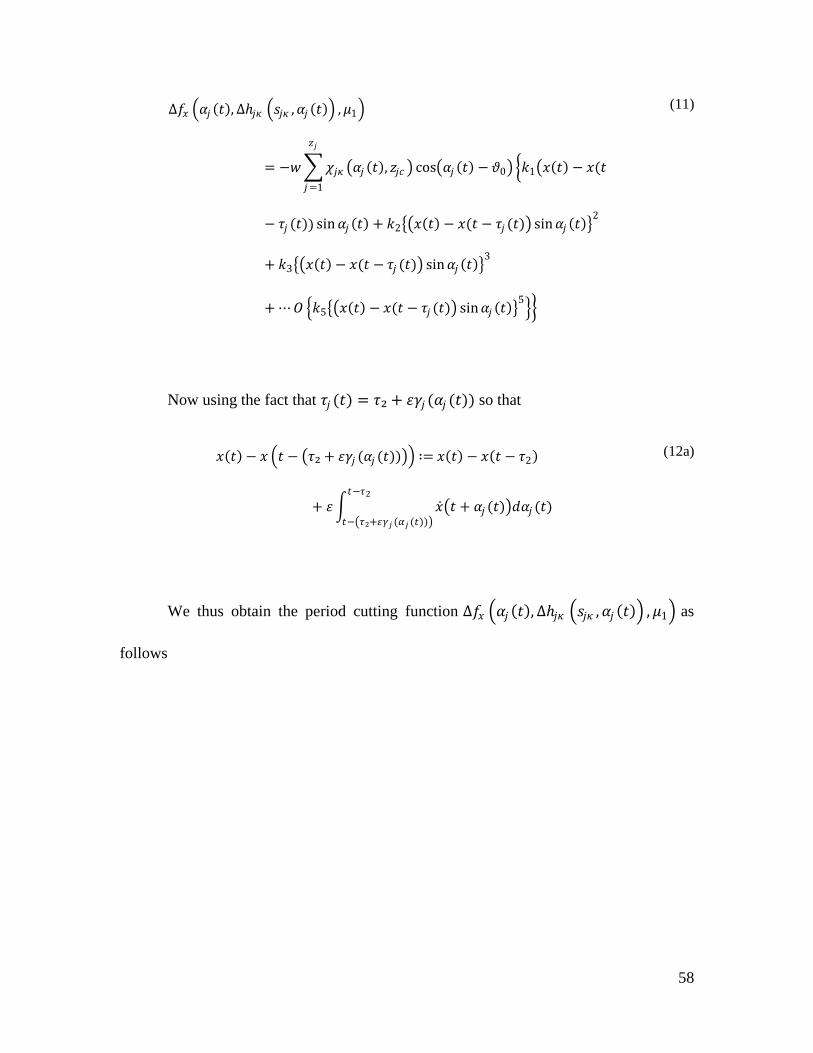
58


= −𝑤𝑤�𝜒𝜒𝑗𝑗𝑗𝑗 �𝛼𝛼𝑗𝑗 (𝑡𝑡), 𝑧𝑧𝑗𝑗𝑐𝑐 �

𝑧𝑧𝑗𝑗

𝑗𝑗=1

cos�𝛼𝛼𝑗𝑗 (𝑡𝑡) − 𝜗𝜗0� �𝑘𝑘1�𝑥𝑥(𝑡𝑡) − 𝑥𝑥(𝑡𝑡

− 𝜏𝜏𝑗𝑗 (𝑡𝑡)) sin𝛼𝛼𝑗𝑗 (𝑡𝑡) + 𝑘𝑘2��𝑥𝑥(𝑡𝑡) − 𝑥𝑥(𝑡𝑡 − 𝜏𝜏𝑗𝑗 (𝑡𝑡)� sin𝛼𝛼𝑗𝑗 (𝑡𝑡)�2


+⋯𝑂𝑂 �𝑘𝑘5��𝑥𝑥(𝑡𝑡) − 𝑥𝑥(𝑡𝑡 − 𝜏𝜏𝑗𝑗 (𝑡𝑡)� sin𝛼𝛼𝑗𝑗 (𝑡𝑡)�5��

(11)

Now using the fact that 𝜏𝜏𝑗𝑗 (𝑡𝑡) = 𝜏𝜏₂ + 𝜀𝜀𝛾𝛾𝑗𝑗 (𝛼𝛼𝑗𝑗 (𝑡𝑡)) so that

𝑥𝑥(𝑡𝑡) − 𝑥𝑥 �𝑡𝑡 − �𝜏𝜏₂ + 𝜀𝜀𝛾𝛾𝑗𝑗 (𝛼𝛼𝑗𝑗 (𝑡𝑡))�� ∶= 𝑥𝑥(𝑡𝑡) − 𝑥𝑥(𝑡𝑡 − 𝜏𝜏2)


𝑡𝑡−�𝜏𝜏₂+𝜀𝜀𝛾𝛾𝑗𝑗 (𝛼𝛼𝑗𝑗 (𝑡𝑡))�

(12a)

We thus obtain the period cutting function ∆𝑓𝑓𝑥𝑥 �𝛼𝛼𝑗𝑗 (𝑡𝑡),∆ℎ𝑗𝑗𝑗𝑗 �𝑠𝑠𝑗𝑗𝑗𝑗 ,𝛼𝛼𝑗𝑗 (𝑡𝑡)� , 𝜇𝜇1� as

follows

59


= −𝑤𝑤�𝑘𝑘1 �𝑥𝑥(𝑡𝑡) − 𝑥𝑥(𝑡𝑡 − 𝜏𝜏2) + 𝜀𝜀 � �̇�𝑥�𝑡𝑡 + 𝛼𝛼𝑗𝑗 (𝑡𝑡)�𝑑𝑑𝛼𝛼𝑗𝑗 (𝑡𝑡)𝑡𝑡−𝜏𝜏2

𝑡𝑡−�𝜏𝜏₂+𝜀𝜀𝛾𝛾𝑗𝑗 (𝛼𝛼𝑗𝑗 (𝑡𝑡))��

+ 𝑘𝑘2 �𝑥𝑥(𝑡𝑡) − 𝑥𝑥(𝑡𝑡 − 𝜏𝜏2) + 𝜀𝜀 � �̇�𝑥�𝑡𝑡 + 𝛼𝛼𝑗𝑗 (𝑡𝑡)�𝑑𝑑𝛼𝛼𝑗𝑗 (𝑡𝑡)𝑡𝑡−𝜏𝜏2


2

+ 𝑘𝑘3 �𝑥𝑥(𝑡𝑡) − 𝑥𝑥(𝑡𝑡 − 𝜏𝜏2) + 𝜀𝜀 � �̇�𝑥�𝑡𝑡 + 𝛼𝛼𝑗𝑗 (𝑡𝑡)�𝑑𝑑𝛼𝛼𝑗𝑗 (𝑡𝑡)𝑡𝑡−𝜏𝜏2


3

+ ⋯𝑂𝑂�𝑘𝑘5 �𝑥𝑥(𝑡𝑡) − 𝑥𝑥(𝑡𝑡 − 𝜏𝜏2)



5

��

(12b)

where the time-varying regenerative delay 𝜏𝜏𝑙𝑙�𝛼𝛼𝑗𝑗 (𝑡𝑡), 𝑧𝑧𝑗𝑗𝑐𝑐 ,Ω� is defined by

⎩⎪⎨

⎪⎧ 𝜏𝜏𝑗𝑗 �𝛼𝛼𝑗𝑗 (𝑡𝑡), 𝑧𝑧𝑗𝑗𝑐𝑐 ,Ω� = 𝜏𝜏2 + 𝜀𝜀𝛾𝛾 �𝛼𝛼𝑗𝑗 (𝑡𝑡)� , 0 ≤ 𝜀𝜀 ≪ 1

𝛾𝛾 �𝛼𝛼𝑗𝑗 (𝑡𝑡)� = � 𝑏𝑏𝑚𝑚(1) cos𝜔𝜔𝑚𝑚 𝛼𝛼𝑗𝑗 (𝑡𝑡)

∞

𝑚𝑚=0

+ � 𝑏𝑏𝑚𝑚(2) sin𝜔𝜔𝑚𝑚 𝛼𝛼𝑗𝑗 (𝑡𝑡)

∞

𝑚𝑚=1

�

(12c)

and the Fourier constants 𝑏𝑏𝑚𝑚(0), 𝑏𝑏𝑚𝑚

(1)and 𝑏𝑏𝑚𝑚(2), namely

60

⎩⎪⎪⎪⎪⎪⎪⎪⎪⎨

⎪⎪⎪⎪⎪⎪⎪⎪⎧ 𝑏𝑏𝑚𝑚

(0) =1

Γ�𝛼𝛼𝑗𝑗 (𝑡𝑡), 𝑧𝑧𝑗𝑗𝑐𝑐 ,Ω�∙

� �� 𝑏𝑏𝑚𝑚(1) cos𝜔𝜔�𝑚𝑚 𝛼𝛼𝑗𝑗 (𝑡𝑡)

∞

𝑚𝑚=0

+ � 𝑏𝑏𝑚𝑚(2) sin𝜔𝜔�𝑚𝑚 𝛼𝛼𝑗𝑗 (𝑡𝑡)

∞

𝑚𝑚=1

�𝑑𝑑𝛼𝛼𝑗𝑗 (𝑡𝑡)

Γ�𝛼𝛼𝑗𝑗 (𝑡𝑡),𝑧𝑧𝑗𝑗𝑐𝑐 ,Ω�

0

𝑏𝑏𝑚𝑚(1) =

1Γ�𝛼𝛼𝑗𝑗 (𝑡𝑡), 𝑧𝑧𝑗𝑗𝑐𝑐 ,Ω�

∙


∞

𝑚𝑚=0


∞

𝑚𝑚=1

� cos𝜔𝜔�𝑚𝑚 𝛼𝛼𝑗𝑗 (𝑡𝑡)𝑑𝑑𝑡𝑡


0

𝑏𝑏𝑚𝑚(2) =

1Γ�𝛼𝛼𝑗𝑗 (𝑡𝑡), 𝑧𝑧𝑗𝑗𝑐𝑐 ,Ω�

∙


∞

𝑚𝑚=0


∞

𝑚𝑚=1

� sin𝜔𝜔�𝑚𝑚 𝛼𝛼𝑗𝑗 (𝑡𝑡)𝑑𝑑𝑡𝑡


0

�

(12d)

Substituting Equations (6) and (12) into (1), and using only the linear part of Equations (6)

we obtain the following equation

�̈�𝑥 + 2𝜁𝜁𝜔𝜔0�̇�𝑥 + 𝜔𝜔02𝜇𝜇1�𝑥𝑥 − 𝑥𝑥(𝑡𝑡 − 𝜏𝜏1)� +𝜔𝜔0

2𝜇𝜇2�𝑥𝑥 − 𝑥𝑥(𝑡𝑡 − 𝜏𝜏2)�

= −𝜀𝜀𝜔𝜔02𝜎𝜎3 �𝑥𝑥 − 𝑥𝑥(𝑡𝑡 − 𝜏𝜏2) + � �̇�𝑥(𝑡𝑡 + 𝜃𝜃)𝑑𝑑𝜃𝜃

𝑡𝑡−𝜏𝜏2

𝑡𝑡−𝜏𝜏(𝑡𝑡)�

3

− 𝑂𝑂(𝜀𝜀5)

(13)

where 𝜀𝜀𝜎𝜎3 denotes the presence of the nonlinearity of the cutting force variation

We study the linear stability of this equation so as to establish regimes of stable

milling process and safe coolant penetration forces.

5.4. Linear Stability Analysis

The linear stability of Equation (12) is examined by considering the linearized

solutions to the delay differential equation

61

�̈�𝑥 + 2𝜁𝜁𝜔𝜔0�̇�𝑥 +𝜔𝜔02𝑥𝑥 + 𝜔𝜔0

2𝜇𝜇1�𝑥𝑥 − 𝑥𝑥(𝑡𝑡 − 𝜏𝜏1)� + 𝜔𝜔02𝜇𝜇2�𝑥𝑥 − 𝑥𝑥(𝑡𝑡 − 𝜏𝜏2)� = 0 (13a)

whose transcendental characteristic equation is

𝛥𝛥(𝜆𝜆, 𝜇𝜇1, 𝜇𝜇2) ∶= 𝜆𝜆2 + 2𝜁𝜁𝜔𝜔0𝜆𝜆 + 𝜔𝜔02 + 𝜔𝜔0

2�𝜇𝜇1�1− 𝑒𝑒−𝜆𝜆𝜏𝜏1� + 𝜇𝜇2 �1 − 𝑒𝑒−𝜆𝜆𝜏𝜏2� � = 0 (13b)

is obtained after making the substitutions 𝑥𝑥(𝑡𝑡) = 𝑒𝑒𝑥𝑥𝑒𝑒(𝜆𝜆𝑡𝑡) , 𝑥𝑥(𝑡𝑡 − 𝜏𝜏) = 𝑒𝑒𝑥𝑥𝑒𝑒(𝜆𝜆(𝑡𝑡 − 𝜏𝜏))

and 𝜏𝜏 ∈ [𝜏𝜏₁, 𝜏𝜏₂] . The force coefficient 𝜇𝜇₁ is considered as the bifurcation that is

continuously perturbed by a small value 𝜀𝜀𝜇𝜇₁ at its critical value 𝜇𝜇1𝑐𝑐 and we write 𝜇𝜇₁ =

𝜇𝜇1𝑐𝑐 + 𝜀𝜀𝜇𝜇 . By Hopf bifurcation conditions [21-22] and reference cited therein, we

let 𝜆𝜆1,2 = 𝜐𝜐(𝜇𝜇₁) ± 𝑗𝑗𝜔𝜔(𝜇𝜇₁) , 𝑗𝑗 = √−1 with 𝜐𝜐(𝜇𝜇₁) > 0 , 𝜔𝜔(𝜇𝜇₁) ≠ 0 and 𝜐𝜐(𝜇𝜇1𝑐𝑐) = 0 ,

ℜ𝑒𝑒{𝑑𝑑𝛥𝛥(𝜆𝜆, 𝜇𝜇₁, 𝜇𝜇₂)/𝑑𝑑𝜇𝜇₁} ≠ 0 be the eigenvalues of (4b). All the remaining eigenvalues of

𝛥𝛥(𝜆𝜆, 𝜇𝜇₁, 𝜇𝜇₂) = 0 have negative real parts. Then, the substitution of 𝜆𝜆₁ = 𝜐𝜐(𝜇𝜇₁) + 𝑗𝑗𝜔𝜔(𝜇𝜇₁)

into 𝛥𝛥(𝜆𝜆, 𝜇𝜇₁, 𝜇𝜇₂) = 0, and setting the real and imaginary parts of the resulting algebraic

equations to zero, we have

𝛥𝛥(𝜆𝜆, 𝜇𝜇1, 𝜇𝜇2) ∶= 𝐺𝐺111(𝜆𝜆, 𝜇𝜇1, 𝜇𝜇2) + 𝑗𝑗𝑀𝑀111 (𝜆𝜆, 𝜇𝜇1, 𝜇𝜇2) = 0, 𝑗𝑗 = √−1 (14a)

where the symbols 𝐺𝐺₁₁₁(𝜆𝜆, 𝜇𝜇₁, 𝜇𝜇₂) and 𝑀𝑀₁₁₁(𝜆𝜆, 𝜇𝜇₁,𝜇𝜇₂) denote the real and imaginary parts

accordingly

�𝐺𝐺₁₁₁(𝜆𝜆, 𝜇𝜇₁, 𝜇𝜇₂) ∶= 𝑣𝑣2 +𝜔𝜔0

2 −𝜔𝜔2 + 2𝜁𝜁𝜔𝜔0𝑣𝑣 + 𝜔𝜔02 �𝜇𝜇1�1− 𝑒𝑒−𝜆𝜆𝜏𝜏1 cos𝜔𝜔𝜏𝜏1� +𝜇𝜇2 �1 − 𝑒𝑒−𝜆𝜆𝜏𝜏2 cos𝜔𝜔𝜏𝜏2�

� = 0

𝑀𝑀111 (𝜆𝜆, 𝜇𝜇1, 𝜇𝜇2): = 2(𝑣𝑣 + 𝜁𝜁𝜔𝜔0)𝜔𝜔− 𝜔𝜔0 2 �𝜇𝜇1𝑒𝑒−𝜆𝜆𝜏𝜏1 sin𝜔𝜔𝜏𝜏1 + 𝜇𝜇2𝑒𝑒−𝜆𝜆𝜏𝜏2 sin𝜔𝜔𝜏𝜏2� = 0

� (14b)

62

and by putting 𝜐𝜐 = 0 at Hopf bifurcation yields

�𝐺𝐺₁₁₁(𝜆𝜆, 𝜇𝜇₁, 𝜇𝜇₂) ∶= 𝜔𝜔0

2 −𝜔𝜔2 + 𝜔𝜔02{𝜇𝜇1(1− cos𝜔𝜔𝜏𝜏1) + 𝜇𝜇2 (1 − cos𝜔𝜔𝜏𝜏2) } = 0

𝑀𝑀111 (𝜆𝜆, 𝜇𝜇) ∶= 2𝜁𝜁𝜔𝜔0𝜔𝜔 − 𝜔𝜔0 2 {𝜇𝜇1 sin𝜔𝜔𝜏𝜏1 + 𝜇𝜇2 sin𝜔𝜔𝜏𝜏2} = 0

� (14c)

or equivalently

�𝜔𝜔0

2𝜇𝜇1(1 − cos𝜔𝜔𝜏𝜏1) = −{(𝜔𝜔0 2 −𝜔𝜔2) +𝜔𝜔0

2 𝜇𝜇2 (1− cos𝜔𝜔𝜏𝜏2)}𝜔𝜔0

2𝜇𝜇1 sin𝜔𝜔𝜏𝜏2 = 2𝜁𝜁𝜔𝜔0𝜔𝜔− 𝜔𝜔02𝜇𝜇2 sin𝜔𝜔𝜏𝜏2

� (14d)

Now squaring both sides of Equations (14d) and adding the result together will

lead to

2𝜔𝜔04𝜇𝜇1

2(1− cos𝜔𝜔𝜏𝜏1)

= {(𝜔𝜔0 2 −𝜔𝜔2) + 𝜔𝜔0

2 𝜇𝜇2 (1− cos𝜔𝜔𝜏𝜏2)}2 + {2𝜁𝜁𝜔𝜔0𝜔𝜔 − 𝜔𝜔02𝜇𝜇2 sin𝜔𝜔𝜏𝜏2}2

(15a)

where the substitution of the first equation in (14d) into (15a), namely

2𝜔𝜔02𝜇𝜇1{(𝜔𝜔0

2 −𝜔𝜔2) + 𝜔𝜔0 2 𝜇𝜇2 (1− cos𝜔𝜔𝜏𝜏2)}

= {(𝜔𝜔0 2 −𝜔𝜔2) + 𝜔𝜔0

2 𝜇𝜇2 (1 − cos𝜔𝜔𝜏𝜏2)}2 + {2𝜁𝜁𝜔𝜔0𝜔𝜔 −𝜔𝜔02𝜇𝜇2 sin𝜔𝜔𝜏𝜏2}2

(15b)

and thus we obtain the explicit expression for the bifurcation parameter 𝜇𝜇₁

𝜇𝜇1(𝜏𝜏1, 𝜏𝜏2,𝜔𝜔, 𝜇𝜇2) =1

2𝜔𝜔0 2 𝜋𝜋112

(𝜋𝜋1112 + 𝜋𝜋112

2 ) (15c)

63

with 𝜋𝜋₁₁₁ and 𝜋𝜋₁₁₂ donating

�𝜋𝜋₁₁₁ = −{(𝜔𝜔0

2 −𝜔𝜔2) + 𝜔𝜔0 2 𝜇𝜇2 (1 − cos𝜔𝜔𝜏𝜏2)}

𝜋𝜋₁₁₂ = 2𝜁𝜁𝜔𝜔0𝜔𝜔 − 𝜔𝜔02𝜇𝜇2 sin𝜔𝜔𝜏𝜏2

� (15d)

We compute Hopf's transversality condition by differentiating implicitly (13b)

with respect to 𝜇𝜇₁, namely

𝑑𝑑𝑑𝑑𝜇𝜇1

{∆(𝜆𝜆, 𝜇𝜇1, 𝜇𝜇2)} =𝑑𝑑∆(𝜆𝜆, 𝜇𝜇1, 𝜇𝜇2)

𝑑𝑑𝜆𝜆×𝑑𝑑𝜆𝜆𝑑𝑑𝜇𝜇1

+𝑑𝑑∆(𝜆𝜆, 𝜇𝜇1, 𝜇𝜇2)

𝑑𝑑𝜇𝜇1= 0

(16a)

from which the real and imaginary parts when 𝜆𝜆1,2 = 𝜐𝜐(𝜇𝜇₁) ± 𝑗𝑗𝜔𝜔(𝜇𝜇₁) are given by

�𝑑𝑑𝜆𝜆𝑑𝑑𝜇𝜇1

�𝜆𝜆1,2=𝜐𝜐(𝜇𝜇₁)±𝑗𝑗𝜔𝜔 (𝜇𝜇₁)

= �− �𝑑𝑑∆(𝜆𝜆, 𝜇𝜇1,𝜇𝜇2)

𝑑𝑑𝜇𝜇1��

𝑑𝑑∆(𝜆𝜆, 𝜇𝜇1, 𝜇𝜇2)𝑑𝑑𝜆𝜆 �

−1


= �−𝜔𝜔0

2 (1− cos𝜔𝜔𝜏𝜏1 + 𝑗𝑗 sin𝜔𝜔𝜏𝜏1)𝜋𝜋113 + 𝑗𝑗𝜋𝜋114

�𝜆𝜆1,2=𝜐𝜐(𝜇𝜇1)±𝑗𝑗𝜔𝜔 (𝜇𝜇1),𝜐𝜐(𝜇𝜇1𝑐𝑐)=0

∶= �𝐺𝐺222 (𝜆𝜆, 𝜇𝜇1,𝜇𝜇2) + 𝑗𝑗𝑀𝑀222 (𝜆𝜆, 𝜇𝜇1, 𝜇𝜇2)}𝜆𝜆1,2=𝜐𝜐(𝜇𝜇1)±𝑗𝑗𝜔𝜔 (𝜇𝜇1),𝜐𝜐(𝜇𝜇1𝑐𝑐)=0

(16b)

where by writing

64

�𝑑𝑑𝜆𝜆𝑑𝑑𝜇𝜇1


= �−𝜔𝜔0

2 (1− cos𝜔𝜔𝜏𝜏1 + 𝑗𝑗 sin𝜔𝜔𝜏𝜏1)𝜋𝜋113 + 𝑗𝑗𝜋𝜋114


∶= �𝐺𝐺222 (𝜆𝜆, 𝜇𝜇1, 𝜇𝜇2) + 𝑗𝑗𝑀𝑀222 (𝜆𝜆, 𝜇𝜇1,𝜇𝜇2)}𝜆𝜆1,2=𝜐𝜐(𝜇𝜇1)±𝑗𝑗𝜔𝜔 (𝜇𝜇1),𝜐𝜐(𝜇𝜇1𝑐𝑐)=0

(16c)

with the notations 𝜋𝜋₁₁₃, 𝜋𝜋₁₁₄, 𝐺𝐺₂₂₂(𝜆𝜆, 𝜇𝜇₁, 𝜇𝜇₂), 𝑀𝑀₂₂₂(𝜆𝜆, 𝜇𝜇₁,𝜇𝜇₂):

⎩⎪⎨

⎪⎧𝐺𝐺₂₂₂(𝜆𝜆, 𝜇𝜇₁, 𝜇𝜇₂) = −

1𝜋𝜋113

2 + 𝜋𝜋1142 �𝜔𝜔0

2�(1 − cos𝜔𝜔𝜏𝜏1)𝜋𝜋113 + sin𝜔𝜔𝜏𝜏1 𝜋𝜋114��

𝑀𝑀₂₂₂(𝜆𝜆, 𝜇𝜇₁, 𝜇𝜇₂) = −1

𝜋𝜋1132 + 𝜋𝜋114

2 �𝜔𝜔02�(1− cos𝜔𝜔𝜏𝜏1)𝜋𝜋114 − sin𝜔𝜔𝜏𝜏1 𝜋𝜋113��

�

(16d)

�𝜋𝜋113 = 2𝜁𝜁𝜔𝜔0 + 𝜔𝜔0

2𝜏𝜏1𝜇𝜇1 cos𝜔𝜔𝜏𝜏1 + 𝜔𝜔02𝜏𝜏2𝜇𝜇2 cos𝜔𝜔𝜏𝜏2

𝜋𝜋114 = 2𝜔𝜔 − 𝜔𝜔02𝜏𝜏1𝜇𝜇1 sin𝜔𝜔𝜏𝜏1 + 𝜔𝜔0

2𝜏𝜏2𝜇𝜇2 sin𝜔𝜔𝜏𝜏2�

(16e)

and thus it can be seen that

ℜ�𝑑𝑑𝜆𝜆𝑑𝑑𝜇𝜇1


= 𝐺𝐺222 (𝜆𝜆, 𝜇𝜇1, 𝜇𝜇2)𝜆𝜆1,2=𝜐𝜐(𝜇𝜇1)±𝑗𝑗𝜔𝜔 (𝜇𝜇1),𝜐𝜐(𝜇𝜇1𝑐𝑐)=0 > 0 (16f)

if the choice of values for the model parameters are such that the inequality (16g) holds.

𝜔𝜔02�(1 − cos𝜔𝜔𝜏𝜏1)𝜋𝜋113 + sin𝜔𝜔𝜏𝜏1 𝜋𝜋114� < 0 (16g)

This means that the pair of eigenvalues 𝜆𝜆₁, ₂ = 𝜐𝜐(𝜇𝜇₁) ± 𝑗𝑗𝜔𝜔(𝜇𝜇₁) of 𝛥𝛥(𝜆𝜆, 𝜇𝜇₁, 𝜇𝜇₂) =

0 with 𝜐𝜐(𝜇𝜇1𝑐𝑐) = 0, 𝜔𝜔(𝜇𝜇1𝑐𝑐) ≠ 0 will cross the imaginary axis from left to right in the

complex plane with a nonzero speed as the bifurcation parameter 𝜇𝜇₁ varies near its

65

critical value 𝜇𝜇1𝑐𝑐 . Also, it ensures that the steady state stability of the system is lost

at 𝜇𝜇₁ = 𝜇𝜇1𝑐𝑐 .

We derive the explicit expression for 𝜏𝜏₂ by rewriting equations (5d) as follows

𝜔𝜔02(1− cos𝜔𝜔𝜏𝜏1)𝜔𝜔0

2𝜇𝜇1 sin𝜔𝜔𝜏𝜏1= −

𝜔𝜔02 −𝜔𝜔2 + 𝜔𝜔0

2𝜇𝜇2(1 − cos𝜔𝜔𝜏𝜏2)2𝜁𝜁𝜔𝜔0𝜔𝜔 − 𝜔𝜔0

2𝜇𝜇2 sin𝜔𝜔𝜏𝜏2=𝜋𝜋111

𝜋𝜋112

(17a)

or equivalently

1 − cos𝜔𝜔𝜏𝜏₁sin𝜔𝜔𝜏𝜏₁

=𝜋𝜋111

𝜋𝜋112

(17b)

where using the fact that cos²𝜔𝜔𝜏𝜏₁ + sin²𝜔𝜔𝜏𝜏₁ = 1 and the trigonometric identity

𝑡𝑡𝑚𝑚𝑛𝑛(𝜔𝜔𝜏𝜏₁

2) = �

sin2 𝜔𝜔𝜏𝜏₁2

cos2 𝜔𝜔𝜏𝜏₁2

= �1/2(1 − 𝑐𝑐𝑧𝑧𝑠𝑠𝜔𝜔𝜏𝜏₁)1/2(1 + 𝑐𝑐𝑧𝑧𝑠𝑠𝜔𝜔𝜏𝜏₁)

= �(1 − 𝑐𝑐𝑧𝑧𝑠𝑠𝜔𝜔𝜏𝜏₁)(1− 𝑐𝑐𝑧𝑧𝑠𝑠𝜔𝜔𝜏𝜏₁)(1 + 𝑐𝑐𝑧𝑧𝑠𝑠𝜔𝜔𝜏𝜏₁)(1− 𝑐𝑐𝑧𝑧𝑠𝑠𝜔𝜔𝜏𝜏₁)

= �(1 − 𝑐𝑐𝑧𝑧𝑠𝑠𝜔𝜔𝜏𝜏₁)²

(𝑠𝑠𝑒𝑒𝑛𝑛²𝜔𝜔𝜏𝜏₁)= �

(1 − 𝑐𝑐𝑧𝑧𝑠𝑠𝜔𝜔𝜏𝜏₁)𝑠𝑠𝑒𝑒𝑛𝑛𝜔𝜔𝜏𝜏₁ � =

1 − 𝑐𝑐𝑧𝑧𝑠𝑠𝜔𝜔𝜏𝜏₁𝑠𝑠𝑒𝑒𝑛𝑛𝜔𝜔𝜏𝜏₁

(17c)

so that

�𝜔𝜔𝜏𝜏1

2� = 𝑚𝑚𝜋𝜋𝑐𝑐𝑡𝑡𝑚𝑚𝑛𝑛 �

𝜋𝜋111

𝜋𝜋112�+ 𝜋𝜋𝑗𝑗, 𝑗𝑗 = ,1,2,3,⋯𝑛𝑛,⋯ (17d)

and thus we obtain

66

𝜏𝜏₁ =2𝜔𝜔

{𝑚𝑚𝜋𝜋𝑐𝑐𝑡𝑡𝑚𝑚𝑛𝑛(𝜋𝜋111

𝜋𝜋112) + 𝜋𝜋𝑗𝑗}, 𝑗𝑗 = ,1,2,3,⋯𝑛𝑛,⋯ (17e)

and with 𝜏𝜏₁ = 2𝜋𝜋/(𝑧𝑧𝑐𝑐Ω), we get the spindle expression

Ω =2𝜋𝜋𝑧𝑧𝑐𝑐𝜏𝜏1

=𝜋𝜋𝜔𝜔

tan−1 �𝜋𝜋111𝜋𝜋112

�, 𝑗𝑗 = ,1,2,3,⋯𝑛𝑛,⋯ (17f)

Using Equations (15) and (17), we obtain the stability charts as presented in

Figure 25 and Figure 26 for the following cases: 1) cutting without cutting fluids, 2)

cutting with cutting fluids. All the stability charts are plotted using Matlab and the

constants selected are listed below [33].

Natural Frequency 𝜔𝜔0 = 6038.7 𝐻𝐻𝑧𝑧

Damping Factor 𝜁𝜁 = 0.025%

Nominal Time Delay for Cutting Fluid Factor 𝜏𝜏2 = 3.5 × 10−4

67

Figure 25: Stability lobes - Cutting without cutting fluid [2 flutes, 3 flutes and 4 flutes]

Figure 26: Stability lobes - Cutting with varying penetration force of cutting fluid

High Speed Region

68

Chapter 6. Results and Discussions

Based on the study and the stability charts we obtain, a correlation between

process regenerative chatter and the penetration force of cutting fluid is observed and

quantified as follows:

1) The study shows that the end mill with more flutes delivers better stability

regimes. However for machining soft material like aluminum, fewer flutes are preferred

to remove chips continuously. The result points to the selection of three flutes for

widening the stability regimes.

2) In high speed machining (Spindle speed > 6000RPM), when we assumed that

all the other machining constants and variables are not changed and the penetration force

of cutting fluid is more significant than other disturbance factors, increased penetration

force of the cutting fluid will reduce the stability region of the machining proportionally.

3) From the stability chart, we observe that dry machining at high spindle speed is

preferred within our model. However, the use of cutting fluid is necessary in order to

control the machining temperature and remove chips continuously. Generally, these

disturbance factors such as the temperature, lubrication and chips were not considered in

this research.

4) The accurate selection of the penetration force of the cutting fluid is of great

importance if one is to balance among the concerns of regenerative chatter, cutting fluid

contaminants, penetration forces and high temperatures.

69

Several preceding studies were also reviewed to compare with our results

obtained here. Ezugwu et al. [42] have tried to machine nickel-base Inconel 718 alloy

with ceramic tools under finishing conditions with various coolant supply pressures. In

their experiment, they cut the same material with three sets of cutting speed: 200 m/min,

270 m/min and 300 m/min and two sets of feed rate: 0.1 mm/rev and 0.2 mm/rev while

the depth of cut was held always. The cutting fluid they used for trials was a high

lubricity emulsion coolant containing alkanolamine salts of the fatty acid and

dicyclohexylamine. The concentration of the coolant was six percent. Then they applied

three different pressure of cutting fluid: 11 MPa, 15 MPa and 20.3 MPa. Cutting forces,

tool life, surface roughness and surface integrity were four considerations as results of the

trials. Some of the results were reported based on their experiment: Lower tool life were

generated when machining with the highest pressure of the coolant jet (20.3 MPa) and

accelerated notch wear on both flank and rake faces of the ceramic tool during machining

were more significant when increasing the pressure of the coolant jet. Both of these

results will reflect our analytical results to some extent. And lower cutting forces were

generated when machining at higher coolant supply due to improved cooling and

lubrication at the cutting interface and as a result of chip segmentation caused by the high

pressure coolant jet. For cutting force, another similar research has done by

Mazurkiewicz et al. [43]. They cut 1020 steel for all the trials with different pressure of

coolant: 70 MPa, 140 MPa, 210 MPa and 280 MPa. Their results (Figure 27) showed that

when increasing the pressure of the coolant jet proportionally, the cutting force was

reduced mainly due to the cooling and lubrication enhancement. However it should be

paid attention that the decreasing speed (slope) was significantly slowed when increasing

70

the coolant pressure. This phenomenon was not specified and analyzed in their research.

And it could be highly possible to be caused by the results from our model. Besides both

Mazurkiewicz et al. and Sharma et al. [44] have mentioned respectively in their papers

that the cooling and lubrication of the tool-chip interface by the coolant jets can account

for the reduction in friction in the contact region between the tool and the workpiece and

the generation of the short curl chip which may also affect the machining stability.

Figure 27: Cutting force under different pressure of coolant

To fully understand the impact of the penetration force of the cutting fluid and its

correlation with machining stability for wide-range materials would require the analysis

of nonlinear effect. The study of nonlinear effect is a recommended future work.

0

100

200

300

400

500

600

700

800

900

70 140 210 280

Fx

71

Chapter 7. Conclusion

Today, there are increasing efforts to discover ways to optimize machining

processes. Among all the manufacturing processes, machining creates great financial

wealth. With the rapid advancement of numerically controlled machine tools and the

ability to design and simulate complex machining task with CAD/CAM software, high

speed milling operations, for example, now provide industries an opportunity to remove

substantial volumes of materials at super high feeds and spindle speeds. In this thesis, we

have established a direct correlation between the penetration force of the cutting fluid and

stability of the milling process at specific spindle speeds. A mathematical model is

constructed and the governing equations are derived in terms of the cutting conditions,

the coolant penetration force and mass flow rate. Stability charts are constructed with and

without the penetration force of the coolant. It is found that by increasing the penetration

force of the coolant, the machining stability regimes become narrow when other

machining variables are assumed not to be changed. The study also shows how changing

number of the flutes impact stable spindle speed. It is discovered that the use of higher

number of flutes in process milling expands the regimes of stability.

72

References

1. Aronson, R. B. Machine Tool 101: Part 6, Machine Servers. Manufacturing

Engineering. 6 1994, pp. 47-52.

2. Iowa Waste Reduction Center. Cutting Fluid Management - Small Machining

Operations. Cedar Falls, Iowa : s.n., 2003.

3. Koelsch, J. R. Honing Fluid Performance. Manufacturing Engineering. 2 1994, pp.

51-55.

4. Bienkowski, K. Coolants & Lubricants - The Truth. Manufacuturing Engineering. 3

1993, pp. 90-96.

5. Foltz, G. Definitions of Metalworking Fluids. 1990.

6. Oberg, E., et al. Machinery's Handbook. New York City, NY : Industrial Press Inc.,

1992. p. 2543.

7. Stocker, W. M. and Hicks, T. Metalcutting: Today's Techniques for Engineers and

Shop Personnel. s.l. : McGraw-Hill, 1979. p. 182.

8. Hope, D. A. Cutting fluids - Pet or pest. Tribology International. 2 1977, pp. 23-27.

9. Tuholski, R. J. Don't Forget the Cutting Fluid. Journal of Industrial Technology. Fall

1993, pp. 2-5.

10. Wikipedia.org. Cutting fluid - Wikipedia, the free encyclopedia. Wikipedia. [Online]

2 13, 2010. [Cited: 4 11, 2010.] http://en.wikipedia.org/wiki/Cutting_fluid.

73

11. The Essential for Choosing the Right Cutting Fluid. Valcool, V. s.l. : Modern

Application News, 9 2002.

12. Hoobler, G. L. Coolant Management: A User's Introduction and Guide to Waste

Minimization.

13. Cassin, C. and Boothroyd, G. Lubrication action of cutting fluids. Journal of

Mechanical Engineering Science. 3 1965, Vol. 7, pp. 67-81.

14. El-Hofy, Hassan. Fundamentals of Machining Processes. Boca Raton, Florida : CRC

Press, 2007. 0849372887.

15. Lopez de Lacalle, L. N., et al. Recording of real cutting forces along the milling of

complex parts. Mechatronics. 2006, Vol. 16, 21-32.

16. Lopez de Lacalle, L. N., et al. Using high pressure coolant in the drilling and turning

of low. International Journal of Advanced Manufacturing Technology. 2000, Vol. 16, 85-

91.

17. Tobias, S. A. Machine tool vibration. London, England : Blackie, 1965.

18. Tlustly, J. Dynamics of high speed milling, handbook of high speed. London,

England : Champman and Hall, 1985.

19. Smith, K. S. and Dvorak, D. Tool path strategies for high speed milling.

Mechatronics. 1998, Vol. 8, 291-300.

20. Chiriacescu, S. T. Stability in the Dynamics of Metal Cutting. New York : Elsevier,

1990.

74

21. Fofana, M. S. Delay dynamical systems and applications to machine-tool chatter.

Chaos, Solitons and Fractals. 2003, Vol. 17, 731-747.

22. Fofana, M. S., et al. Illustrative applications of the theory of delay dynamical

systems. Mathematical and Computer Modeling. 2003, Vol. 37, 1371-1382.

23. Fofana, M. S. Moment Lyapunov exponent of a stochastic delay equation.

International Journal of Mathematics and Mathematical Sciences. 6, 2002, Vol. 30, 339-

351.

24. Fofana, M. S. Sufficient conditions for the stability of single and multiple

regenerative chatter. Chaos, Solitons and Fractals. 2002, Vol. 14, 335-347.

25. Fofana, M. S. Aspects of stable and unstable machining by Hopf bifurcation. Journal

of Applied Mathematical Modeling. 2002, Vol. 26, 953-973.

26. Fofana, M. S. Spatial decomposition in a mechanical system with discrete delays.

International Journal of Differential Equations and Applications. 4, 2000, Vol. 4, 371-

395.

27. Fofana, M. S. Effects of time delays near center manifold. International

Mathematical Journal. 3, 2002, Vol. 1, 285-302.

28. Fofana, M. S. and Lamb, D. L. On the stability of a nonlinear time delay system.

Automatica Journal. 3, 1995, Vol. 34, 375-378.

29. Fofana, M. S., Ee, K. C. and Jawahir, I. S. Machining stability in turning operation

when cutting with a progressively worn tool insert. Wear. 2003, Vol. 255, 1395-1403.

75

30. Fofana, M. S. and Ryba, P. B. Parametric stability of nonlinear time delay equations.

International Journal of Nonlinear Mechanics. 2003, Vol. 39, 79-91.

31. Hanna, N. H. and Tobias, S. A. A theory of nonlinear regenerative chatter. ASME

Journal of Engineering for Industry. 1974, Vol. 96, 247-255.

32. Shi, H. M. and Tobias, S. A. Theory of finite amplitude machine instability.

International Journal of Machine Tool Design and Research Conference. 1, 1984, Vol.

24, 45-69.

33. Tobias, S. A. Machine Tool Vibration. London : Blackie and Sons Ltd, 1965.

34. Manufacturing Engineering, Aerospace and Defense Manufacturing. s.l. : Society of

Manufacturing Engineers, 2008.

35. Heisel, Uwe and Mult, H. C. Production engineering, research and development.

Annals of the German Academic Society for Production Engineering. 2, 2006, Vol. 13.

36. Vieira, J. M., Machado, A. R. and Ezugwu, E. O. Performance of cutting fluid

during face milling of steels. Journals of Material Process Technology. 2001, Vol. 116,

244-251.

37. Xavior, M. A. and Adithan, M. Determining the influence of cutting fluids on tool

wear and surface roughness during turning of AISI 304 austenitic stainless steel. Journal

of Material Process Technology. 2009, Vol. 209, 900-909.

38. Belluco, W. and De Chiffre, L. Performance evaluation of vegetable-based oil in

drilling austenitic stainless steel. Journal of Materials Process Technology. 2004, Vol.

148, 171-176.

76

39. Axinte, D. A. and De Chiffre, L. Effectiveness and resolution of tests for evaluating

the performance of cutting fluids in machining aerospace alloys. CIRP Annals -

Manufacturing Technology. 2008, Vol. 57, 129-132.

40. Sales, W. F., et al. Evaluation of Cutting Fluids Using Scratch Tests and Turning

Process. Journal of the Brazil Society of Mechanical Science and Engineering. 2007, Vol.

29, 372-378.

41. Axinte, D., Axinte, M. and Tannock, J. D. A multicriteria model for cutting fluid

evaluation. Proceedings of the Institution of Mechanical Engineers, Part B: Journal of

Engineering Manufacture. 2003, Vol. 217, 1341-1353.

42. Ezugwu, E. O., et al. Machining of nickel-base, Iconel 718, alloy with ceramic tools

under finishing conditions with various coolant supply pressures. Journal of Materials

Processing Technology. 2005, Vols. 162-163, 609-614.

43. Mazurkiewicz, M., Kubala, Z. and Chow, J. Metal machining with high-pressure

water-jet cooling assistance - a new possibility. Journal of Engineering for Industry. 1989,

Vol. 111, 7-12.

44. Sharma, C. S., Rice, W. B. and Salmon, R. Some effects of injecting cutting fluids

directly into the chip-tool interface. Journal of Engineering for Industry. 1971, Vol. 93,

441-444.

45. Taylor, F. W. On the art of cutting metals. The Transaction of ASME. 1906, Vol. 28,

70-350.

the correlation between the penetration force of cutting ... · the correlation between the...

Documents