the convection dispersion equation - not the question, the
TRANSCRIPT

Copyright is owned by the Author of the thesis. Permission is given for a copy to be downloaded by an individual for the purpose of research and private study only. The thesis may not be reproduced elsewhere without the permission of the Author.

The Convection Dispersion Equationnot the Question, the Answer!
Anion land Cation Transport through Undisturbed Soil Columns
during Unsaturated Flow
A thesis presented in partial fulfilment of the requirements for
the degree of
Doctor of Philosophy in Soil Science
at Massey University
Iris Vogeler
1997

i i
Abstract
Prediction of solute movement through the unsaturated zone is important in determining
the risk of groundwater contamination from both "natural" and surface applied
chemicals. In order to understand better the mechanisms controlling this water-borne
transport, unsaturated leaching experiments were carried out on undisturbed soil
columns, about 3 l itres in volume, for two contrasting soils. One was the weakly
structured Manawatu fine sandy loam, and the other the well-aggregated Ramiha silt
loam. Anion transport was satisfactorily described using the convection dispersion
equation CCDE), provided that anion exclusion for the Manawatu soil, and adsorption
for the Ramiha soil were taken into account. At water flux densities of about 3 mm h·l,
a dispersivity of about 40 mm was obtained for the Manawatu soi l , and a dispersivity of
about 15 mm for the Ramiha soi l . The difference was probably due to the contrasting
structures of the two soils. Increasing the water flux density in the Manawatu soil to
about 13 mm hoI resulted in a slightly higher dispersivity of about 60 mm.
Flow interruption resulted in a subsequent drop in the effluent concentration for the
Manawatu soil but not in the Ramiha soil . This suggests that the lag time for transverse
molecular diffusion from "mobile" to "immobile" water domains was important in the
Manawatu soi l, but not in the Ramiha soil.
In both soils cation transport was described satisfactorily with the CDE in conjunction
with cation exchange theory, providing that only 80% of the cations replaced by 1 M
ammonium acetate were assumed to be involved in exchange reactions.
Column leaching experiments were also carried out using a rainfall simulator and larger
columns of about 22 litres of the Manawatu soil with a short pasture on top. Solid
chemical was applied to both a dry and a wet soil surface. Neither the pasture nor the
initial water content had a significant effect on solute movement. Slightly higher
dispersivities of about 70 mm were found.

i i i
Time Domain Reflectometry (TDR) was found to be valuable for monitoring solute
transport in a repacked soil under transient water flow conditions. But in undisturbed
soils TDR only proved to be accurate under steady-state water flow when absolute
values of solute concentration were not sought.
The CDE was thus found to satisfactorily answer the question of how to describe
transport of non-reactive and reactive solutes under bare soi l and under short pasture.
This applied during both steady-flow and transient wetting.

IV
Acknowledgements
Thanks to god for creating such a wonderful soil , and for taking the time to separate the
soil water into "mobile" and "immobile" fractions (or not?).
Special thanks to David Scotter for his excellent supervision, understanding and
encouragement throughout my study. Dave, aside from being an expert in the field of
soil physics, was always concerned for my future and well-being. Apart from tons of
help and advice, he showed plenty of patience in watching bubbles throughout sleepless
nights.
Thanks also to Brent Clothier for his patient discussion and constructive criticisms
during the research and writing of my thesis, as wel l as for his friendship.
Appreciation and thanks are also extended to Russell Tillman and Steven Green .
Steve' s introduction to the TDR-system and modell ing was much appreciated.
The Department of Soil Science and the Environment Group of HortResearch as a
whole have always been friendly, and gave help whenever I needed it.
Finally I would like to express my gratitude to my parents, brother and also to Shane for
their love and support.

v
Table of Contents
Abstract
Acknowledgements
Table of Contents
List of Tables
List of Figures
List of Symbols
CHAPTER 1
1. INTRODUCTION 1
1.1 The Purpose of the Study 2
1.2 The Experimental Procedure of the Study 5
1.3 The Structure of the Study 6
CHAPTER 2
2. THE THEORY OF SOLUTE MOVEMENT IN SOILS 9
2.1 Introduction 9
2.2 Micro- and Macroscopic Views 9
2.2. 1 Representative Elementary Volume and Representative Elementary Area 1 1 2.2.2 Flux and Resident Concentrations 1 2
2.3 The Language of Models 14
2.3 . 1 Transfer Function Approach 1 4 2.3.2 Partial Differential Equations 1 9
2.4 Stochastic-Convective Approaches 20
2.4. 1 Convective-Lognormal Transfer Function 2 1 2.4.2 Burns' Leaching Equation 22 2.4.3 Transfer Function Approach l inked with the Hydraulic Conductivity-Water
Content Relationship 22
ii IV V x
x
xvi
vi
2.5 Convective-Dispersive Approach 23
2.5. 1 Convection-Dispersion Equation as a Partial Differential Equation 24 2.5.2 Convection-Dispersion Equation as a Transfer Function Model 25 2.5.3 Bolt 's Approach for Describing Solute Dispersion 27
2.6 The Mobilellmmobile Model 30
2.6. 1 MobilelIrnrnobile Approach as a Partial Differential Equation 30 2.6.2 MobilelIrnrnobile Approach as a Transfer Function 3 1 2.6.3 Critique on the MobilelIrnrnobile Approach 3 1 2.6.4 The Link Between the MobilelIrnrnobile Approach and Bolt 's Approach 33
2.7 Layer and Mixing Cell Models 34
2.8 Reactive Solutes 34
2.8. 1 Solute Adsorption 35 2.8.2 Cation Transport 37
2.9 Boundary Conditions and Solutions for the Convection-Dispersion Equation 42
2.9. 1 Flux and Resident Concentrations 42 2.9.2 Boundary and Initial Conditions 43 2.9.3 Analytical Solutions 46 2.9.4 Numerical Solutions 47
2.10 Classification of Solute Transport Models 49
2.11 Conclusions 51
CHAPTER 3
3. THE THEORY OF TIME DOMAIN REFLECTOMETRY FOR MEASURING
SOIL WATER CONTENT AND SOLUTE CONCENTRATION 53
3.1 Introduction 53
3.2 The Measurement System 55
3.3 TDR for Measuring Soil Moisture Content 57
3.4 TDR for Measuring Solute Concentration 60
3.5 TDR for Monitoring Water and Solute Transport 64
3.6 Probe Configuration and Sensitivity 65
3.7 Installation of Transmission Lines 66
3.8 Conclusion 67

vii
CHAPTER 4
4. TIME DOMAIN REFLECTOMETRY: CALIBRATION AND ITS USE TO
MONITOR SOLUTE TRANSPORT 68
4.1 Introduction 68
4.2 Characterising Water and Solute Movement by TDR and Disk Permeametry 69
4.2. 1 Abstract 69 4.2.2 Introduction 69 4.2.3 Theory 70 4.2.4 Materials and Methods 73
4.2.4. 1 Use of TDR 73 4.2.4.2 Soil Material 75 4.2.4.3 TDR Calibration 75 4.2.4.4 Positive Charge Measurement 76 4.2.4.5 Column Experiment 76
4.2.5 Results and Discussion 79 4.2.5 . 1 Water-Content Calibration 79 4.2.5.2 Solute-Concentration Calibration 80 4.2.5.3 Column Experiment 82
4.2.5 .3. 1 Water Flow 82 4.2.5.3.2 Chloride Movement 83
4.2.6 Conclusions 87
4.3 TDR and Undisturbed Soil Columns of Manawatu Fine Sandy Loam 89
4.4 TDR Estimation of the Resident Concentration of Electrolyte in the Soil Solution 90
4.4. 1 Abstract 90 4.4.2 Introduction 9 1
4.4.3 Theory 92 4.4.4 Materials and Methods 93
4.4.4. 1 TDR Calibration 95 4.4.5 Results 96
4.4.5 . 1 Water Content Calibration 96 4.4.5.2 Solute Concentration Calibration 96 4.4.5.3 Leaching Experiments 98
4.4.6 Conclusions 1 02 L-----'
4.5 Overall Conclusions 104

viii
CHAPTER 5
5. ANION MOVEMENT THROUGH UNSATURATED SOIL 106
5.1 Introduction 106
5.2 Anion Transport Through Intact Soil Columns During Intermittent Unsaturated Flow 108
5.2. 1 Abstract 1 08
5.2.2 Introduction 1 08
5.2.3 Theory 1 1 0
5 .2.4 Materials and Methods 1 1 3 5 .2.5 Results and Discussion 1 1 5
5 .2.5 . 1 Water Flow and Storage 1 1 5 5 .2.5.2 Chloride and Nitrate in the Effluent and S imulation Results using
the CDE 1 17 5 .2.5.3 Resident Solute Concentrations and Simulation Results using
the CDE 1 1 8
5 .2.5.4 Characterising Anion Movement using Suction Cup Data 1 1 9 5 .2.5.5 Characterising Anion Movement using TDR 1 2 1 5 .2.5.6 Simulation using the Mobilellmmobile Model 1 22
5 .2.6 Conclusions 1 24
5.3 Solute Movement through Undisturbed Soil Columns Under Pasture during Unsaturated Flow 125
5.3 . 1 Abstract 1 25 5.3 .2 Introduction 1 26 5.3.3 Theory 127 5.3.4 Materials and Methods 1 30
5 .3 .4. 1 Column Experiments 1 30 5 .3 .4.2 Chemical Analysis 1 3 1 5 .3 .4.3 Rainfall S imulator 1 32
5 .3 .5 Results 1 34 5 .3 .5 . 1 Anion Movement 1 34 5 .3 .5.2 Resident Concentrations of Strontium 1 36
5 .3 .6 Discussion 1 37 5.3 .6. 1 Conclusions 1 3 8
5.4 Bolt's Approach and Anion Transport 139
5.5 Overall Conclusions 140

ix
CHAPTER 6
6. CATION MOVEMENT THROUGH UNSATURATED SOIL 143
6.1 Introduction 143
6.2 Cation Transport During Unsaturated Flow Through Two Intact Soils 144
6.2. 1 Summary 1 44 6.2.2 Introduction 1 44 6.2.3 Theory 1 46 6.2.4 Methods and Materials 1 49 6.2.5 Results and Discussion 1 50
6.2.5 . 1 Cation Exchange Capacity and Selectivity Coefficients 1 50 6.2.5.2 Anion Movement 1 53 6.2.5.3 Calcium and Magnesium Outflow 1 56 6.2.5.4 Resident and Solution Concentrations of Calcium and Magnesium 1 60 6.2.5.5 Suction Cup Measurements 1 62 6.2.5.6 Leaching of Potassium 1 63
6.2.6 Conclusions 'rb5 6.3 Cation Movement and the MobilelImmobile Concept 166
6.4 Overall Conclusions 167
7. GENERAL CONCLUSIONS
REFERENCES
APPENDIX A
CHAPTER 7
A. l Numerical Solutions for the CDE used in this Study A. l . 1 Non-reactive Solutes A. l .2 Numerical S imulations for the Mobilellmmobile Approach A. l .3 Numerical Simulation of Cation Movement
APPENDIX B
B. l Program 1 B.2 Program 2 B.3 Program 3 B.4 Program 4 B .5 Program 5
169
174
193
1 93 1 93 1 94 1 95
202
202 205 207 209 2 1 2

List of Tables
Chapter 4
Table 4 .1 Column data and model parameters obtained from the CDE. ------------ 94
Chapter 5
Table 5.1 Transport parameters obtained as described in the text. ------------------- 115
Table 5 .2 Parameters from column leaching experiments on Manawatu fine sandy
loam using the CDE, the MIM, and Bolt 's approach. --------------------- 140
Fig. 2 .1
Fig. 2 .2
Fig. 2 .3
Fig. 2 .4
Fig. 2 .5
List of Figures
Chapter 2
Simplified picture of the soil with macropores of various sizes, and soil
matrix with rnicropores. -------------------------------------------------------- 10
Flux concentration (Cf) and resident concentration (Cr). ------------------ 13
Column leaching experiment with breakthrough-curves for non-
reactive and reactive solutes, and anion exclusion. ------------------------ 15
Comparison between simulations using the CDE and MIM, based on
the approach of Bolt (1982), eq. [2 .37] . ------------------------------------- 33
Exchange isotherms for a homovalent system with cation species A and B for various values of the selectivity coefficient KA-S. -------------- 39
x

Fig. 2.6
Fig. 2.7
Fig. 2.8
Fig. 3. 1
Fig. 3.2
Fig. 4. 1
Fig. 4.2
Fig. 4.3
Fig. 4.4
BTC's for a homovalent system with cation species A and B for
various values of KA-B for (a) an unfavourable isotherm, and (b) a
favourable isotherm. ------------------------------------------------------------ 40
Flux (solid l ines) and resident concentrations (broken lines) for two
different Pelect numbers. ------------------------------------------------------ 42
Numerical gri d. ------------------------------------------------------------------ 48
Chapter 3
Schematic diagram of the TDR system. ------------------------------------- 56
An idealized TDR voltage trace vs. time. ----------------------------------- 57
Chapter 4
Diagram of the combined TDR and disk permeameter set-up. ----------- 77
Volumetric water content determined gravimetrically vs. TDR
measured dielectric constant. Also shown is the fitted function, and
the empirical relationship suggested by Topp et al. ( 1 980). -------------- 80
TDR-measured bulk soil electrical conductivity vs. electrical
conductivity of the soil solution measured with a conductivity meter
for different water contents of Ramiha silt loam. -------------------------- 8 1
TDR-measured water content for the vertically- and the horizontally
installed probe vs. time during infiltration. --------------------------------- 83
Xl

Fig. 4.5
Fig. 4.6
Fig. 4.7
Fig. 4.8
Fig. 4.9
The resident concentration estimated from the TDR-measured bulk
soil electrical conductivity of the horizontally-installed probe during
infiltration of KCl . -------------------------------------------------------------- 85
The electrical conductivity of the soil solution calculated from the TDR
measured bulk soil electrical conductivity of the vertically-installed probe
during infi ltration of KCl . ----------------------------------------------------- 86
The anion exchange capacity measured for various concentrations of
KCI in the soil solution. -------------------------------------------------------- 87
TDR-measured bulk soil electrical conductivity vs. electrical conductivity
of the soil solution measured with a conductivity meter for different water
contents for Manawatu fine sandy loam using disturbed and undisturbed
soil columns. ----------------------------------------------------------------------- 97
Normalised bulk soil electrical conductivity as measured by TDR and
simulated curves for column A and column B. Also shown are the
normalised resident concentrations calculated with values obtained from
measurements on disturbed or undisturbed columns. ------------------------ 99
Xll
Fig. 4. 1 0 Normalised anion breakthrough data and fitted curves using the CDE for
column C and column D. --------------------------------------------------------- 100
Fig. 4. 1 1 Normalised bulk soil electrical conductivity as measured by TDR and
simulated curves for column C and column D. Also shown are the
normalised resident concentrations calculated from TDR------------------- 1 0 1

Fig. 5 . 1
Fig. 5 .2
Fig. 5 .3
Fig. 5 .4
Fig. 5.5
Fig. 5 .6
Fig. 5.7
Fig. 5.8
xii i
Chapter S
Experimental setup of the leaching experiment under pasture, including the
rainfall simulator. ------------------------------------------------------------------ 1 07
Measured outflow flux density as a function cumulative infiltration for
columns A and column B . -------------------------------------------------------- 1 16
Normalized anion breakthrough data and fitted curves using the CDE at the
low flow rate for column A and column B, and for column B at the high flow
rate. ---------------------------------------------------------------------------------- 1 17
Anion concentrations in the soil solution inferred from soil extracts for
column A and column B . --------------------------------------------------------- 1 19
(a) Normalised anion breakthrough data measured by suction cups and
simulated curves for column A and column B .
(b) Normalised bulk soil electrical conductivity as measured by TOR and
simulated curves for column A and column B. ------------------------------- 1 20
Normalized anion breakthrough data and fitted curves using the mobile/
immobile approach of the CDE at the low flow rate for column A and
column B, and for column B at the high flow rate. --------------------------- 1 23
Diagram of the rainfall simulator. -------------------------------------------- 1 33
Normalised anion breakthrough data and fitted curves using the CDE for
Column I, and column II with solute either applied to a wet surface or a
dry surface as a function of cumulative drainage. ---------------------------- 1 35

Fig. 5 .9
xiv
Concentrations of Sr2+ in column I at the end of the experiment, as obtained
from large samples and subsamples. Also shown are the simulations using
the CDE in conjunction with cation exchange theory. ---------------------- 1 37
Fig. 5 . 1 0 Simplified picture of the soil with mobile, immobile and excluded
Fig. 6. 1
Fig. 6.2
Fig. 6.3
Fig. 6.4
water. -------------------------------------------------------------------------------- 1 4 1
Chapter 6
(a) Ammonium-acetate measured CEC, at the soil ' s pH, as obtained for
columns A, B, C, and D, and independent measurements from the field
for Manawatu and Ramiha soil as a function of depth.
(b) and (c) Initial relative concentrations of exchangeable cations from
field measurements. ------------------------------------------------------------- 1 5 1
Relative amounts of charge on the exchange sites balanced by different
cations as a function of the relative concentration in the soil solution
for (a) the Ca-Mg-system, and (b) the K-(Ca + Mg)-system for the
Manawatu fine sandy loam. --------------------------------------------------- 1 53
Normalized anion breakthrough data during leaching and prediction
using the CDE (a) for Manawatu soil columns A and column B, and
(b) for Ramiha soil for columns C and D. (c) resident anion
concentrations as a function of depth for Manawatu soil and Ramiha.
Also shown are the predictions. ----------------------------------------------- 1 54
Effluent concentrations of Ca2+ and Mg2+ as a function of cumulative
infiltration for columns A, B, C, and D. Also shown are the simulations
assuming the total measured CEC is involved and only 80% of the
ammonium-acetate measured CEC is involved. ---------------------------- 1 57

Fig. 6.5
Fig. 6.6
Fig. 6.7
Fig. 6.8
xv
Relative concentrations on the exchange sites of XCa and XMg at the end of
the experiment for columns A, B, C, and D. Also shown are the simulations
using 80 % and 1 00% of the ammonium-acetate measured CEC. ------- 1 6 1
Measured concentrations C from the suction cups for Ca2+ and Mg2+
as a function of cumulative infiltration for columns A and B . Also
shown are the simulations using 80 % of the ammonium-acetate
measured CEC. ------------------------------------------------------------------ 1 62
(a) Effluent concentrations for K+ during leaching with Ca(N03)2 solution
and MgCl2 solution as a function of cumulative infiltration for columns A,
B, C, and D. Also shown for the Manawatu soil are the simulations using
80% of the ammonium-acetate measured CEC, and a KK-CM value of
3. 1 (mol m·3) 112 .
(b) Measured concentrations of K+ on exchange sites for columns A, and
B, and initial K+ concentrations for the Manawatu soi l . Also shown are the
simulated concentrations.
(c) Measured concentrations of K+ on exchange sites for columns C, and
D, and initial K+ concentrations for the Ramiha soil . ---------------------- 1 64
Effluent concentrations of Ca2+ and Mg2+ as a function of cumulative
infiltration for columns A and B. Also shown are the simulations using
the mobilelimmobile approach of the CDE and assuming only 80% of
the ammonium-acetate measured CEC is involved. ----------------------- 1 67

XVI
List of Symbols
Roman Symbols
a empirical constant [m3 kg- I ]
a i , a2 variables in computer program
b empiricaJ constant
bl, b2 variabJes in computer program [kg or mol m-3]
C propagation of an electromagnetic wave in free space [m S-I]
C I , C2 variables in computer program [(mol m-3)2]
C3 empirical constant
d empirical constant
I fraction of exchange sites in immobile water domain
Ie temperature correction coefficient
!t(Q) solute probability function of cumulative infi ltration [m- I ]
!t(t) solute travel-time probability function [S-I ]
g solute life-time probability function [S- I ]
ho pressure head [m]
L column length or cal ibration length [m]
La apparent TDR probe length [m]
Lt TDR probe length [m]
n constant in Eq. 2.22 and Eq. 2.40
qd diffusional flux exchange between mobile and immobile
water [kg or mol m-2 S- I ]
qi solute flux in immobile phase [kg or mol m-2 S- I ]
qrn solute flux in mobile phase [kg or mol m-2 S- I ]
qw water flux density [m S-I ]
qs solute flux density [kg or mol m-2 S- I ]
r voltage reflection coefficient
t time [s]
t' input time [s]
v pore water velocity [m S- I ]

xvii
Vp relative velocity setting on TDR instrument
Ve propagation velocity of an electromagnetic pulse [m S- I ]
x variable in computer program [kg or mol m-3]
y variable in computer program [kg or mol m-3]
z depth [m]
As cross-sectional area [m2]
A ion species
B ion species
C concentration in soil solution [kg or mol m-3]
Ca(z) depths-dependent initial soil solution concentration [kg or mol m-3]
Cai total initial anion concentration [kg or mol m-3]
CA concentration of cation species A in soil solution [kg or mol m-3]
CB concentration of cation species A in soil solution [kg or mol m -3]
Cr flux-averaged solute concentration [kg or mol m-3]
Ci resident soil solution concentration in immobile phase [kg or mol m-3]
Cm resident soil solution concentration in mobile phase [kg or mol m-3]
Co(t) time-dependent input solution concentration [kg or mol m-3]
Cr resident soil solution concentration [kg or mol m-3]
Cs soil solution concentration of ion species s [kg or mol m-3]
CT total cation concentration in soil solution [kg or mol m-3]
C1 constant concentration [kg or mol m-3]
Ds hydrodynamic dispersion coefficient [m2 S-I ]
Di diffusion coefficient in soil [m2 S-I ]
Dm dispersion coefficient in mobile phase [m2 S- I ]
Dw soil water diffusivity [m2 S- I ]
Do diffusion coefficient in water [m2 S- I ]
Fin solute mass flux entering soil volume [kg or mol S- I ]
Fex solute mass flux leaving soil volume [kg or mol S-I ]
I ionic strength
Ie convective solute flux in mobile water [kg or mol m-2 S- I ]

Jdisp JE
h KA-B
KM-D
Kd
KG
Ks
Kw
LD
Ldiff
Ldis
Lmim
Mo
M
Mi
Mm
p R
Rc
RH
Rs
Q R
S
SS
T Vo
Vf
Vi
Vr
dispersive solute flux in mobile water
diffusional flux exchange between mobile and immobile
water
longitudinal diffusional flux
selectivity coefficient for cation species A and B
selectivity coefficient in Gapon equation
distribution coefficient
geometric constant of TDR probe
saturated hydraulic conductivity
hydraulic conductivity
diffusion/dispersion length parameter
diffusion length parameter
dispersion length parameter
mobile/immobile exchange length parameter
pulse of solute applied to soil surface
total solute concentration
solute mass in immobile phase
solute mass in mobile phase
Peelet number
retardation factor
radius of cylinders of porous soil
radius of cylindrical macropores
radius of spheres
cumulative drainage or infiltration
solute retardation factor
sorptivity
amount of solute adsorbed
travel time of electromagnetic pulse
zero reference voltage
final reflected voltage at very long time
voltage of incident step
voltage after reflection from probe end
XVlll
[kg or mol m-2 S-I ]
[kg or mol m-2 S- I ]
[kg or mol m-2 S-l]
[(mol kg-3)1I2]
[m3 kg- I ]
[m-I ]
[m S- I ]
[m S- I ]
[m]
[m]
[m]
[m]
[kg or mol m-2]
[kg or mol m-3]
[kg or mol m-3]
[kg or mol m-3]
[m]
[m]
[m]
[m]
[m S- I I2]
[kg or mol kg- I ]
[s]
[V]
[V]
[V]
[V]

XA charge concentration of cation species A on exchanger
XCEC charge concentration of adsorbed cations
Zo characteristic impedance
ZL impedance of TDR probe
Greek Letters
a mass transfer coefficient
f3 constant
8 Dirac delta function
t: dielectric constant
r constant
A dispersivity
Aeff effective dispersivity
Am dispersivity in mobile water
Ameff effective dispersivity in mobile phase
Anum numerical dispersivity
J.11 mean of the lognormal distribution
Ph soil bulk density
(J bulk soil electrical conductivity
OJ variance of the lognormal distribution
(Js surface conductance
(Jw pore water electrical conductivity
l' tortuosity factor
8 volumetric water content
8a residual water content
e. immobile water fraction
8m mobile or effective water fraction
8n initial water content
[mole kg- I ]
[mole kg- I ]
[Q]
[Q]
[S- I ]
[m]
[m]
[m]
[m]
[m]
[s]
[kg m-3]
[S m- I ]
[s]
[S m- I ]
[S m-I ]
[m3 m-3]
[m3 m-3]
[m3 m-3]
[m3 m-3]
[m3 m-3]
xix

saturated water content
excluded water fraction
OJ attenuation coefficient
Subscripts
n depth position
J time index
Ca calcium
D divalent
K potassium
Na sodium
M monovalent
Mg magnesium
CM calcium plus magnesium
Abbreviations
BTC breakthrough curve
CDE convection dispersion equation
CEC cation exchange capacity
CLT convective lognormal transfer function
El expected mean travel time at reference depth I
Ez expected mean travel time at depth z
MIM mobilelimmobile concept
pdf probability density function
REV representative elementary volume
REA representative elementary area
TDR time domain reflectometry
Varl variance at reference depth I
Varz variance at depth z
xx

1
Chapter 1
1. Introduction
Leaching of contaminants such as agricultural chemicals, pesticides, and leachates from
waste disposals and landfills through the unsaturated zone into the underlying
groundwater has become an important area of environmental research worldwide. The
development of models for simulating contaminant transport is a key component for
environmental impact assessment, as it can take decades for groundwater contamination i./' to become apparent . One of the most important parts of solute transport modelling is to
identify the relevant transport processes. Although during recent years much effort has
been directed toward the identification of these processes, it still remains unclear as to
which physical, chemical and biological processes are most important for describing
contaminant transport (Kutflek and Nielsen, 1994). Furthermore the ranking of
importance is likely to be as variable as soils are in Nature !
The recognition of the need to develop solutions for various agricultural and
environmental problems such as pollution of surface and groundwater resources has led
to the development of environmentally-based laws and regulations, such as New
Zealand's Resource Management Act (199 1 ). The regional and district plans within this
Act are directed towards ensuring sustainable surface application of agricultural
chemicals. Irrigation management requires efficient use of water to minimize the
hazardous potential of agrichemicals on the environment, such as the leaching of soil
nutrients into the groundwater. An understanding of the processes affecting solute
transport is necessary to achieve this.
In an attempt to advance the understanding of the transport processes various models
have been proposed (Nielsen and Biggar, 196 1; van Genuchten and Wierenga, 1 986).
Early models considered only non-reactive chemicals, with transport affected only by
convection and dispersion. During the last decade, more and more complex models
have been developed to simulate multispecies transport. However, the relative
capabil ities of existing models and the credibility of their results is still an important
concern (Jury, 1 983; Wagenet, 1983). This is due primarily to the unavailability of

2
appropriate data to confirm the assumptions of these different models and to estimate
their accuracy. Thus, as Engesgaard and Christensen (1988) pointed out: . . . "future
research should be directed towards validation studies . . . rather than developing still
more complex models".
1. 1 The Purpose of the Study
The most-commonly used model to predict solute movement in soil is the convection
dispersion equation (CDE). However despite its widespread use, e validity of the ���� 7
CDE has been questioned. The main concerns are thaYdiffusive mass transfer in
aggregated soils containing immobile water, solute dispersion growth with transport
distance (Khan and Jury, 1990; Jury and Roth, 1 990), and flow down preferential
pathways appear to make it invalid in many situations (Schulin et ai., 1987b).
The CDE has been found to describe satisfactorily one-dimensional solute transport
through homogeneous columns of repacked soil . However in soil columns packed with
large aggregates, or in structured soils, or in the field, the CDE has sometimes been
found wanting (Biggar and Nielsen, 1 976; van Genuchten and Wierenga, 1 976; Nkedi
Kizza et ai., 1 982; White et ai., 1 984) . Solute movement at variance with the CDE has
been explained by nonequilibrium in solution concentration between mobile and
immobile water regions (van Genuchten and Wierenga, 1976), dead end pores, bimodial X pore size distributions (Gerke and van Genuchten, 1 993; Zurmtihl and Durner, 1 996),
and solute diffusion into and out of aggregates. One objective of this study is to
determine if the classical CDE can be used to describe solute transport during
unsaturated flow in undisturbed soils, or alternatively if nonequil ibrium models, such as
the mobile immobile model are needed.
Molecular diffusion and local convection are among the most important processes
affecting solute transport in undisturbed soils (van Genuchten et ai. , 1 988). These
processes are controlled by the structure of the soi l, and in particular the size, shape, and
spacing of the pores. However, as a detailed description of the complex pore geometry
of a soil is not feasible, when the CDE is used the effects of diffusion and dispersion are

3
lumped into a hydrodynamic dispersion coefficient (Rao et ai., 1 980; Brusseau and Rao,
1990). The hydrodynamic dispersion coefficient is often assumed to be linearly related
to the water flow velocity (De Smedt and Wierenga, 1978), with the proportionality
constant termed the dispersivity. However, while the hydrodynamic dispersion caused
by convective transport of solutes is obviously dependent on the velocity of flow,
molecular diffusion occurs at a rate independent of water flow velocity. The question
arises then, can the dispersivity be assumed constant under various water flow rates?
Alternatively does diffusive mass transfer between mobile and immobile water need to
be explicitly considered? In a study on repacked aggregated soils Brusseau (1993)
found the approach of a "lumped" dispersivity, which is velocity invariant, to be
inadequate. Thus another objective of this study is to investigate the effect of the water
flow velocity on solute dispersion in undisturbed soils, and to determine the conditions
under which it is appropriate to use a velocity-invariant dispersivity.
Many studies in the field, and on intact soil cores in the laboratory have revealed a
preferential flow of solutes, that by-passes most of the soil matrix (e.g. Elrick and
French, 1 966; Kissel et al. , 1 973; White et ai., 1984; Beven and German, 1982; Roth et
al. , 1 99 1 ) . This preferential and far-reaching flow of water and solutes is obviously then
of importance in evaluating the potential risk of management practices on the
contamination of the groundwater resources. Whereas by-passing reduces the leaching
of chemicals that are present in the resident soil water, early appearance of surface
applied chemicals in the groundwater may occur, thereby resulting in undesirable
pollution, and a lower application efficiency for fertilizers . Preferential flow is
generally attributed to macropores, that are the result of cracks, or channels formed by
plant roots or soil organisms. Significant water flow through macropores however only
occurs when they are water fi l led (Brusseau and Rao, 1 990), such as under ponded or
near-saturated conditions. In New Zealand however leaching is l ikely to occur
predominately under non-ponding unsaturated conditions, and the CDE may then
satisfactorily describe solute transport. So whether or not preferential flow occurs
during unsaturated leaching will also be addressed in this study.

4
Earlier studies suggest that preferential flow can also be induced during transient
wetting of initial ly dry soil (White et ai., 1 986), or by vegetation funelling the incident
water (Saffigna et ai., 1 976; Kanchanasut and Scotter, 1 982). So, the effects of the
initial water content, and of the vegetation on solute transport during unsaturated flow
will also be assessed in this thesis.
Most leaching studies to date have focused on conservative solutes. Little attention has
been devoted to the transport of reactive solutes, such as cations, although the
importance of exchange reactions had been recognized in 1 963 by Biggar and Nielsen.
Studies on cation transport have been largely confined to repacked soil columns,
although the transport of these might be quite different to the transport in structured
soils, due to non-equilibrium effects, which might be either of a chemical or physical
nature. Thus, cation transport in undisturbed soils will also be investigated in thi s study.
A related objective is to assess the ability of the CDE, in conjunction with cation
exchange theory, to describe cation transport through undisturbed soil columns.
A factor l imiting research on the transfer processes in the unsaturated zone is the lack of
adequate instrumentation to measure in situ simultaneously the water content and the
solute concentration. Within the last decade Time Domain Reflectometry (TDR) has
become widely used for measuring the soi l ' s water content. Now TDR is also being
seen as a means by which the changing concentration of electrolyte in the soil solution
can be observed (Kachanoski et ai. , 1 992) . The ability to take measurements
continuously and automatically, in a non-destructive way, makes TDR a potentially
valuable tool for observing solute transport. However, so far application of this
technique to monitor solute transport through structured soils during non steady water
flow remains a largely unmet challenge. Consequently, another objective of this study
was to investigate the feasibility of time domain reflectometry (TDR) to characterize
water and solute movement in the laboratory in both repacked and undisturbed soil
columns .
5
In summary, this study set out to answer the fol lowing three questions:
1 . Can the convection dispersion equation be used to describe solute transport through
undisturbed soil columns under various unsaturated water flow regimes typical in the
field? In particular, under which conditions is the use of the CDE appropriate, and
when do we need more sophisticated models such as the mobilelimmobile water
concept? Is the assumption of a velocity-invariant dispersivity in the CDE
appropriate? Can we use the CDE in conjunction with cation exchange theory to
describe cation movement through undisturbed soi l?
2. How does the soil surface, in particular the vegetative cover, and the initial water
content prior to solute application affect solute transport?
3 . Can we use Time Domain Reflectometry (TDR) to monitor solute transport under
transient and steady-state water flow through repacked and undisturbed soil columns,
and what are the l imitations associated with TDR?
1.2 The Experimental Procedure of the Study
While experiments in both the laboratory and field are needed to understand fully the
processes involved in solute transport (Hutson and Wagenet, 1 995), the studies
described here are confined to controlled laboratory studies. Although field testing of a
transport models is a necessary component of research, if confidence in model
predictions are to be achieved, they have the disadvantage of lack-of-control. Solutes
have to be col lected within the soil using porous cups, low suction lysimeters, or by
destructive sampling. These methods give only local estimates of the solute
concentration which may however vary significantly in space. Also in the field it is
much harder to control, and define the boundary and initial conditions, and so the testing
of a model is troublesome.
Alternatively, laboratory studies on large undisturbed soil columns can provide volume
averaged solute concentrations. Crucial for meaningful average solute transport

6
behaviour is the column size needed. This depends on the scale of variability of the soil,
and especially the soil surface, e.g. the vegetative cover. Furthermore, the control
possible in the laboratory offers the possibility to study in detail the effects of certain
factors, such as the water flow rate, and intermittent leaching events, on solute transport
behaviour.
Although water flow in the field is often transient, over winter, when a large fraction of
the leaching occurs, the amount of water in the soil various little, and the water content
can be considered fairly constant. The leaching experiments described here were hence
mainly carried out under steady-state water flow. However unsteady water flow is also
considered, as solute flow patterns under intermittent water flow might be quite
different, due to solute movement from rapid flow paths into soil micropores or
aggregates. In order to evaluate the likely role and extent of preferential flow under
situations that mimic the field, the leaching experiments described here were carried out
at water contents below saturation.
1.3 The Structure of the Study
The present study is divided into a theoretical part (Chapters 2 and 3) and an
experimental part which includes modelling (Chapters 4, 5 and 6). The literature
relevant to the various parts is reviewed in the appropriate chapters. The experimental
part is presented in the form of papers. These papers have been submitted to various
international journals, and have either already been accepted for publication, or are still
in review. Minor changes have been made to achieve consistency, and the references
have been moved to the end of the thesis. All papers have multiple authorships. The
contribution of the authors was as follows:
Iris Vogeler:
carried out:
Principle Investigator
all the planning and execution
data collection and model development
physical and chemical analysis
manuscript preparation and writing
David R. Scotter:
aided the study by:
Brent E. Clothier:
aided the study by:
Russell W. Tillman:
aided the study by:
Steven R. Green:
aided the study by:
Advisor
discussing methodology and results
data collection
model development
editing and discussion of the manuscripts
Advisor
discussing methodology and results
editing and discussion of the manuscripts
Advisor
discussing methodology and results
Advisor
model development
discussing results
The titles, locations and status of the various papers are as follows:
7
Characterizing Water and Solute Movement by TDR and Disk Permeametry
Chapter 4.2. By Iris Vogeler, Brent E. Clothier, Steven R. Green, David, R. Scotter, and
Russell W. Tillman. Soil Science Society of American Journal, 1996, 60, 5- 1 2.
TDR Estimation of the Resident Concentration of Electrolyte in the Soil Solution
Chapter 4.4. By Iris Vogeler, Brent E. Clothier, and Steven R. Green. Australian Journal of Soil Research, 1997 (3).
Anion Transport through Intact Soil Columns During Intermittent Unsaturated
Flow.
Chapter 5.2. By Iris Vogeler, David R. Scotter, Brent E. Clothier, and Russel W.
Tillman. Soil Technology, in press.

8
Solute Movement through Undisturbed Soil Columns Under Pasture During
Unsaturated Flow.
Chapter 5 .3 . By Iris Vogeler, David R. Scotter, Steven R. Green, and Brent E. Clothier.
Australian Journal of Soil Research, submitted.
Cation Transport During Unsaturated Flow Through Two Intact Soils
Chapter 6.2. By Iris Vogeler, David R. Scotter, Brent E. Clothier, and Russel W.
Tillman. European Journal of Soil Science, submitted
In Chapter 2, the theory of solute transport is described to provide a general
understanding of the mechanisms that govern chemical transport, such as convection,
diffusion, dispersion, anion exclusion, and adsorption. Furthermore various transport
models are considered. The initial and boundary conditions needed to solve the model
equations are described, and analytical and numerical solutions are outl ined. Chapter 3
covers the theory of time domain reflectometry (TDR) to describe water and solute
transport. In Chapter 4 the use of TDR to monitor solute transport through repacked
and undisturbed soil columns is discussed, and consideration is given to difficulties in
solute concentration measurements by TDR. Several previous studies have shown that
the rate of water application affects the leaching of solutes. This is investigated in
Chapter 5, which deals with the transport of anions through undisturbed soil columns
under various water flow regimes. Firstly, solute transport under bare soil is considered
there, and then solute transport under pasture. The role of different transport
mechanisms in affecting solute transport would appear capable of clarification by
intermittent leaching. So experiments incorporating this are also described. Chapter 6
is concerned with the nature, extent, and the way in which cation exchange reactions
influence the leaching of solutes. Finally Chapter 7 summarizes the results and insights
gained during the study. Appendix A describes the numerical solutions used in the main
computer programs, and in Appendix B some of these programs are listed.

9
Chapter 2
2. The Theory of Solute Movement in Soils
2. 1 Introduction
In this chapter various approaches to describe solute transport through soils, wil l be
outlined and compared. Initially the interaction between the soil-solid phase and solute
is assumed to be negligible, and the solute is considered to be conservative with no
decay or production. However as most nutrients and pollutants react chemically with
the soi l , later in the chapter exchange reactions are considered. Although solute
transport in the soil is coupled with the transport of water, the theory of water transport
is not explicitly discussed here. A brief description of water transport under nonsteady
conditions is given in Chapters 4 and 5.
2.2 Micro- and Macroscopic Views
Modelling the transport of solutes through the soil implies some understanding of the
complex soil system and the processes involved. One simplified physical picture of the
soil is shown in Fig. 2.1. The soil is idealised here as a system of larger pores of various
shapes and sizes. These are termed macropores, and are embedded in a soil matrix
containing smaller pores, or micropores. In saturated soils all pores contain water.
However, under unsaturated conditions some fraction of the macropores will no longer
contain nor transmit water. Water and solute move by convection and diffusion through
the soi l . We could assume that only the water in the macropores moves by convection,
and hence is mobile, and that the water in the micropores is effectively immobile. At
the microscopic scale, the convective flow through the macropores is not uniform, but
variable both within pores and between pores of various sizes. These variations in the
flow velocity, and the different pathlengths of water movement induced by tortuosity,
cause mechanical dispersion of a solute within the flow. Furthermore, the macropores
might intersect occasionally, which results in convective interchange of solute between
them, and thereby reduces the dispersion, and affects the way it scales with depth.

10
Solute exchange between the immobile water in the micropores and the mobile water in
the macropores occurs by transverse molecular diffusion. During wetting of dry soils
solute exchange between the two domains may also occur by convection. Depending on
the spacing between the macropores, and the water flow velocity within them, molecular
diffusion could also lead to exchange between the macropores. Longitudinal molecular
diffusion also occurs, tending to reduce concentration gradients in the direction of water
flow. In fact it will be argued later that if the Darcy flux density is less than about
1 mm d-I, this is likely to be the dominant solute-mixing process. The combined effect of
mechanical dispersion, molecular diffusion and convective mixing is termed
hydrodynamic dispersion (Kutflek and Nielsen, 1994).
Fig. 2.1 Simplified picture of the soil with macropores of various sizes, and soil matrix
with micropores. Molecular diffusion is indicated by the spots.

1 1
2.2.1 Representative Elementary Volume and Representative Elementary Area
A description at the microscopic scale of all these processes occurring in the soil system
is not feasible. Solute transport needs to be viewed at a different scale. Bear ( 1 972) introduced the concept of a representative elementary volume (REV). In an REV the
microscopic processes are volume averaged to produce a macroscopic scale
representation of the processes. It is assumed that an REV encompasses all the
microscopic variabilities, thereby allowing the definition of a meaningful average value
of the parameters, or properties of interest. The concept of what constitutes an REV i s
i ntuitive, and depends on the soil ' s properties. To illustrate the idea o f a n REV,
consider the porosity of a soil. At a point with infinitely small volume, the porosity is
either one or zero, depending on whether the point falls into the void (or pore) space, or
into the solid matrix. With increasing sample size, the porosity changes as different
mixes of pores and matrix are incorporated. With further increase in sample size these
variations in the porosity with sample size become smaller. When the size of an REV i s
reached they become "negligible". For porosity measurements soil samples o f about
1 00 cm3
or 1 0-4 m3 are usually found to be representative. Analogously to the REV, the
representative elementary area (REA) is the minimum area needed to provide a
meaningful average value of a cross section of the porosity. It might be argued that for
solute transport the REV and the REA need be larger than for porosity. Solute transport
behaviour depends not only on the porosity but also depends on the pore size
distribution and pore connectedness.
Solute transport is often studied in the laboratory on soil columns, characteri sed by a
length scale of the order of tens of centimeters. This scale has been termed laboratory
scale (Dagan, 1 986). At the laboratory scale, the columns are assumed homogeneous i n
the sense that the irregular pore structure reproduces itself in various parts o f the
column. A point of dispute is how the parameters obtained at the laboratory scale can
be applied to the larger field scale of m or km. When the sample volume is increased
substantially above the laboratory scale, to the field scale, the regional scale, or even the
soil series scale, the rate of change in variability of soil properties i s likely to also
change. Solute transport parameters obtained from field studies have often been found

1 2
to be highly variable (Biggar and Nielsen, 1 976; Jury et al. , 1 982). However the high
variability of solute transport parameters observed by Biggar and Nielsen ( 1 976) would
have been largely due to the ponded conditions in their study. A review by Jury ( 1 983) on various transport studies in the field suggests that the variations in solute velocity
become smaller under non-ponded conditions. Spatial variability can be analysed using
geostatistics. However it is beyond the scope of this study to discuss the spatial
variability occurring at the field scale. A general discussion is given by Kutflek and
Nielsen ( 1 994).
2.2.2 Flux and Resident Concentrations
When describing solute transport through the soil, it is important to distinguish between
solute flux concentrations and solute resident concentrations. In both cases the
concentrations are defined macroscopically. In the case of a resident concentration it is
an average value over an REV, or in case of the flux concentration averaged over an
REA. The resident concentration (Cr) is a volume-averaged concentration, defined as
the mass or number of moles of solute per unit volume of soil solution [kg or mol m-3].
Resident concentrations can be measured by direct soil sampling, or by electrical
resistance measurements, such as Time Domain Reflectometry. In contrast, the flux
concentration (Cf) is a flux-averaged concentration [kg or mol m-3] , and is the ratio of
the solute flux density qs [kg or mol m-2 S- I ] to the water flux density qw [m S-1
or
m3 m-2
S-I] (Kreft and Zuber, 1 978). It is the effective concentration in the moving
water in the soil. Flux concentrations are obtained from the outflow of column leaching
experiments and lysimeter studies. The difference between flux and resident
concentration is illustrated in Fig. 2.2 . The resident concentration represents the solute
concentration in the "mobile", and in the "immobile" water at a certain time. In
contrast, the flux concentration represents only the concentration in the mobile water as
sampled over a certain time period. Thereby Cf is weighted by the velocity at which
water, and so solute move through the various pathways.

1 3
Fig. 2.2 Resident concentration (Cr) and flux concentration (Cr).

1 4
For steady-state water flow a consideration of mass conservation implies that the flux
and resident concentration for nonreactive solutes are related by,
a Cr + q aCf = 0 a t w az
where t is the time [s] and z the depth [m] .
2.3 The Language of Models
[2. 1 ]
Solute transport models are most commonly represented as either transfer functions, or
as partial differential equations (pdes). Whereas pdes can be used for transient water
flow conditions, transfer functions are restricted to steady-state flow, or at least
conditions, where the water flow pathways are not considerably changed and the soil
water content changes l ittle. However, the transfer function approach does offer a
framework within which predictions from different models can be compared.
2.3.1 Transfer Function Approach
In transfer function models, the solute transport processes are based on random
variables, which are characterized by a probability density function (pdf) . A random
variable is a function that assigns either a number (discrete random variable), or a
certain range (continuous random variable) to every outcome. Thereby random
variables have a probabil ity assigned to them. Given a large number of observations the
frequency of a random event will approach a fixed value, which is called the probability
of that event. The probability is hence a measure of the likelihood that an event will
occur. The pdf then describes how probability is distributed over the possible values a
random variable can take, and satisfies the following conditions,

1 5
f(x) �o for all x
J f{x) = 1 [2.2]
where x is a random variable. Other important concepts of a random variable are the
mean, the expected value of x, E(x), and the variance E[x-E(x)f
Process orientated models can also be presented as transfer functions. Transfer function
models are l imited to l inear time-variant systems, which means that at any time the
output is a l inear combination of present and past values of the input. But provided
changes in soil water storage are small, non-steady flow may be described by using a
surrogate variable for time, such as cumulative infiltration or drainage.
1.0 +--+--::r£!_ ..... ----=�
':!.." 0.5 <.>
0.0 +..<.........,.-----.--..---+ 1 2 3
Liqu ld·lIlled pore volumes
nnln�� 6. (
Fig. 2.3 Column leaching experiment with breakthrough-curves for pison flow, non-reactive and
reactive solutes, and anion exclusion.

1 6
Solute transport i s often studied using column leaching experiments. A solution with
solute concentration Cr (O,t), is applied to the surface of a soil column of length l, and
the concentration measured at the exit surface at the base of the column (Cf (l,t)) is
plotted against time, giving a breakthrough curve (BTC). This is shown in Fig. 2.3 for a
non-reactive and a reactive solute. The shape and the position of the BTC provide
information on the physical and chemical properties of the soil. If no mixing between
the initial and incoming solution would occur, the BTC would be a vertical l ine, which
is termed piston flow. A curved BTC indicates mixing. Shifting of the curve to the left
indicates exclusion or bypass from some fraction of the soil solution. Shifting to the
right indicates solute adsorption by the soil solids.
If we denote the solute input flux by Fin(t) [kg or mol S- I ] , and the output flux by FexCt)
[kg or mol S- I ] , we may write FexCt) as the convolution integral of Fin(t) and the lifetime
pdf g (t-t' I n, where t' is the time when the solute entered the system,
I
F'.:x (t) = f g (t - t ' I t ') F:n (t ')d t' o
where Fin and Fex are given by,
F:n (t)= Cr (O, t )qw (0, t) As
F'.:x (t)=Cr (l , t)qw (l, t) A.
[2.3]
[2.4]
where As is the surface area [m2] , which is assumed to be the same for the input and the
output surface, and I is the length of the soil system studied [m] . Note that g in the
above equation may depend on the time of solute application to the surface t' .
Combining the above equations, and assuming steady state water flow leads to the basic
transfer function for conservative solutes,
I
Cr (l, t) = f Cr (O, t' )J; (l, t- t' )dt' [2.5] o
17
where t is a random variable, andit (/, t-t' ) is the travel time probabil ity density function
(pdf) [S- I ] , often termed the impulse-response function. The pdf gives the probabil ity
that a solute, which has been applied to the soil surface at t = 0, will be flowing passed 1 at time t, and characterizes the solute transport properties of the soil . The pdf is based
on the assumption that the solute transport mechanisms are time-independent and
conservative. However by using a lifetime pdf, the effect of physical, chemical or
biological processes, leading to source-sink terms can be included (Jury and Roth,
1990).
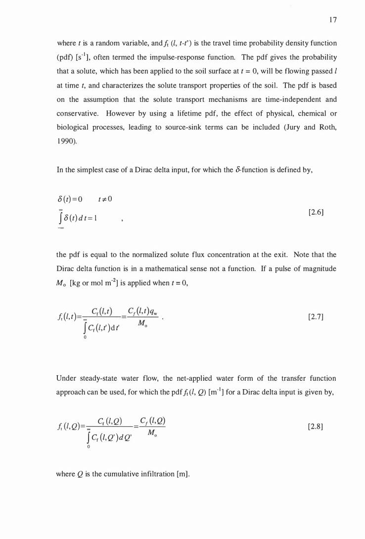
In the simplest case of a Dirac delta input, for which the 8-function is defined by,
8 (t) = 0 t :;t: O
f 8 (t) d t= 1 [2.6]
the pdf is equal to the normalized solute flux concentration at the exit. Note that the
Dirac delta function is in a mathematical sense not a function. If a pulse of magnitude
Mo [kg or mol m-2] is applied when t = 0,
fr (l, t) [2.7]
f Cf (l, t' )d t' o
Under steady-state water flow, the net-applied water form of the transfer function
approach can be used, for which the pdfit (I, Q) [m- I ] for a Dirac delta input is given by,
fr (I, Q)= _ Cf (Z,Q)
f Cf (l, Q' )d Q' o
where Q is the cumulative infiltration [m] .
[2.8]

1 8
Two important properties of a probability density function are the mean and the
variance. The expected value, or mean travel time, E(t), is given by,
�
E{t) = f tf{t) d t [2.9] o
and the variance of t, which describes the mean square deviations of t about the average
value is given by,
�
Var(t) = f [t - E(t)f f(t) dt = E(t 2 ) - E2 (t) . [2. 1 0] o
These two values are unique for any pdf. If the parameters of the pdf are constant in
time and space (i.e . j(l,t) is a stationary function), as well as independent on the type and • -
concentration of solute, then the transfer function is useful as a predictive tool . To
predict solute transport beyond the measurement depth, mechanistic assumptions are
required. Examples will be given in section 2.4 and 2.5.
Transfer functions can be written describing flux and resident concentrations, and for
both flux and resident pulse inputs. The relationship between them is discussed by Jury
and Scotter ( 1 994).
Transfer function models are not restricted to the simple case of the input of a non
reactive solute to the soil surface under steady-state water flow. They also can be used
to simulate the transport of indigenous soil solutes (Magesan et ai., 1 994; Heng et al., 1 994), as well as quasi-transient conditions by using the net-applied water form of the
transfer function equation (Jury and Roth, 1 990), and its pdf [eq. 2.8] . However
implicit in the use of transfer function models to describe solute transport is the
assumption, that the transport properties are not significantly affected by intermittent
drying and wetting cycles. Otherwise water and solute pathways through the soil would
change, and it would not be unique for a particular system. Also, solute transport is
assumed to be a function of the net amount of water applied, but not of the rate at which

1 9
the water i s applied. Linear source and sink terms can be included provided they are
proportional to time or the net amount of water applied (Heng and White, 1 996). For
transport of reactive and non-conservative solutes, Roth and Jury ( 1 993) coupled the
transfer function approach with l inear adsorption kinetics and first order decay.
2.3.2 Partial Differential Equations
Solute transport models are based on conservation and flux laws. The mass
conservation law is given by,
aM + aqs =o a t az
[2. 1 1 ]
where M is the total amount of solute present in a unit volume of soil [kg or mol m-\
As mentioned before, solute movement is due to the combined effect of convective mass
flow of water and molecular diffusion. If convection is the only transport process
operating and both the water flux density and the resident concentration are locally
uniform, then the solute flux density is given by,
[2. 1 2]
The second transport process is molecular diffusion, which always occurs when there
are solute concentration gradients within the pore water. Diffusion of solutes can occur
longitudinally in the direction of flow, thereby increasing the dispersion. This wil l only
be significant at low velocities. If the resident concentration at any depth is not local ly
uniform, molecular diffusion also occurs transverse to the direction of mass flow,
thereby reducing any local concentration differences induced by different local
velocities. Molecular diffusion is described by Fick's first law,

= _ D (} d ( qs I d z
20
[2. 1 3]
where e is the volumetric water content [m3 m-3] , and Di is the effective diffusion
coefficient in the soil [m2 S- I ] , which is related to the diffusion coefficient in water by,
[2. 1 4]
where T is the tortuosity factor, which accounts for the increased pathlength in the soil
compared to the water, and Do is the molecular diffusion coefficient in water. Typically
Do in l iquids is about 1 .5 x 1 0-9 m2 S- I , and T in wet soil is about 0.5. This means that
diffusion occurs over a length scale of mm during time periods of the order of days.
2.4 Stochastic-Convective Approaches
The stochastic-convective approach is consistent with solute movement being solely due
to convection. Stochastic convective transfer functions are consistent with the soil
behaving as if it consists of independent pathways, or stream tubes with different travel
times. Water and solutes move by convection through these tubes. In each tube the
mean velocity v is assumed constant. The various tubes however have different
velocities, the distribution of which is described by a continuous random variable (Jury
et aI., 1 986). Solute mixing between the different tubes is assumed negligible.
The expected or mean travel time is given by,
[2. 1 5]
where Ez and EI are the expected travel times for a certain depth z and the reference
depth I.
2 1
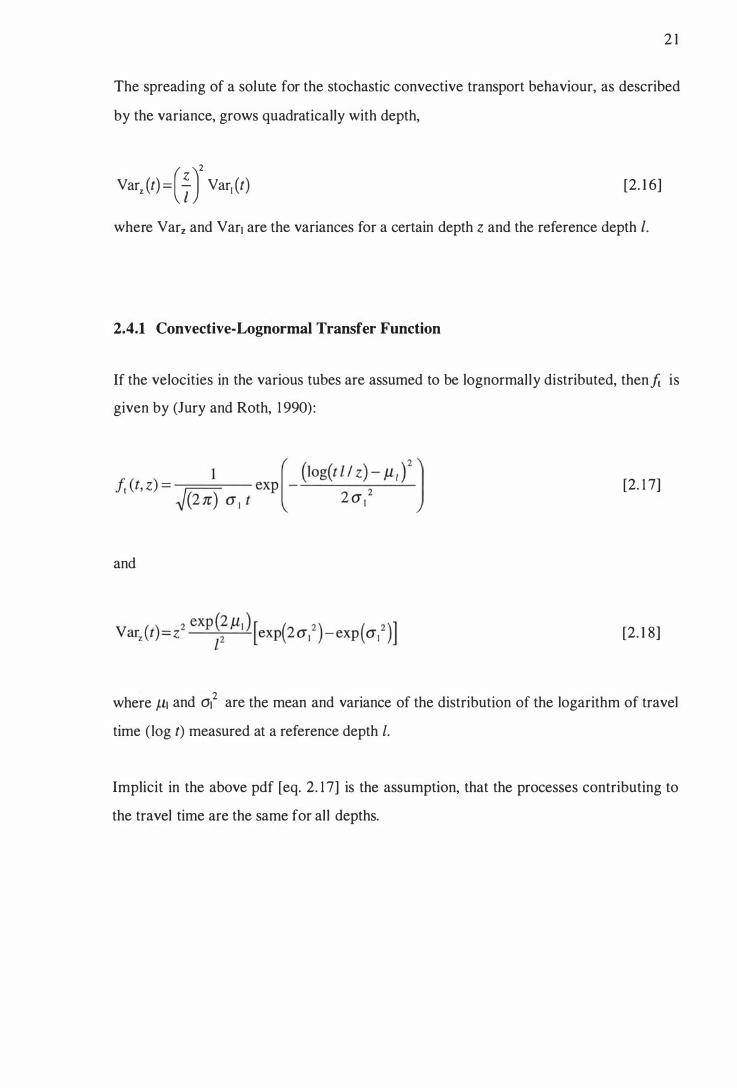
The spreading of a solute for the stochastic convective transport behaviour, as described
by the variance, grows quadratically with depth,
Varz (t) = ( f ) 2 Var, (t) [2. 1 6]
where Varz and Varl are the variances for a certain depth z and the reference depth I.
2.4.1 Convective-Lognormal Transfer Function
If the velocities in the various tubes are assumed to be lognormally distributed, thenft is
given by (Jury and Roth, 1 990):
[2. 1 7]
and
[2. 1 8]
where J.1l and Ol2 are the mean and variance of the distribution of the logarithm of travel
time ( log t) measured at a reference depth I.
Implicit in the above pdf [eq. 2. 1 7] is the assumption, that the processes contributing to
the travel time are the same for all depths.

22
2.4.2 Burns' Leaching Equation
Another stochastic-convective approach is the Bums' leaching equation ( 1 974). Implicit
in the Bums' equation is the following stochastic-convective pdf (Scotter et ai. , 1 993),
( ) (z 8r (-Z8 J f z, Q =Q3 exp Q . [2. 1 9]
2.4.3 Transfer Function Approach linked with the Hydraulic Conductivity-Water Content Relationship
Scotter and Ross ( 1 994) recently suggested that a transfer function derived from the
soi l ' s hydraulic properties could be useful for determining the upper l imit of solute
dispersion . Again solute flow is assumed to be purely convective. The distribution of
the soil water velocities is found from the unsaturated hydraulic conductivity-water
content relationship (K(8» . The velocity distribution is then used to calculate the solute
travel time distribution, thereby giving the travel time probability as,
f(Z, t) = _ _ l d Kw (8) Kw d t
[2.20]
where Kw is the hydraulic conductivity [m S- I ] . However implicit in this approach is the
assumption that the velocity distribution can be inferred from the Kw (8 ) relationship.
This is only true if all the dependence of Kw on 8 is due to flow in the pores emptying or
fil ling, so that the velocity in pores staying filled is unaffected. The irregular geometry
of soil pores might mean this is not always a real istic assumption. Equation [2.20] does
provide an upper limit for the amount of dispersion however, as Scotter and Ross ( 1 994)
suggest.

23
2.5 Convective-Dispersive Approach
In the convective-diffusion approach solute movement is assumed to be due to non
interacting convection and diffusion. Diffusion is described by eq. [2. 1 3] , and
convection by eq. [2. 1 2] , provided that the water flux density (qw) and the solute
resident concentration (C) in the soil are locally uniform. However convection is not
describable by [2. 1 2] , and convection and diffusion interact as described in section 2.2.
In the CDE, the effects of nonuniform qw and diffusion are lumped into the
hydrodynamic dispersion coefficient. Further it is assumed that hydrodynamic
dispersion can mathematically be described as a diffusion-like process, with the total
solute flux given by,
[2 .2 1 ]
where Ds is the hydrodynamic dispersion coefficient [m2 S- I ] .
If this equation i s valid, the solute flow can be called convective-dispersive. The
velocity of flow partly determines which of the dispersion processes dominates;
mechanical dispersion, molecular diffusion, or convective mixing. Under fast enough
flow rates, longitudinal molecular diffusion will be small compared to mechanical
dispersion (Gardner, 1 965). The dispersion coefficient is then approximately
proportional to the pore water velocity (Campbell , 1 985). The shape of a BTC
measured for non-reactive solutes should then be independent on the pore water
velocity. However for slow flow, diffusion is often considered as a main mechanism of
dispersion. Diffusion should be independent of water flow, so if it is important, the
shape of the BTC does depend on the pore water velocity.
The velocity-dependency of the hydrodynamic dispersion coefficient (Ds) IS often
described by (De Smedt and Wierenga, 1 978; Brusseau, 1 993),
[2.22]

24
where A. is the dispersivity [m] , v is the pore water velocity defined by qw / e [m s- ' ] , and
n is a constant, often assumed to be one (Hutson and Wagenet, 1 995)_
2.5.1 Convection-Dispersion Equation as a Partial Differential Equation
Combining the solute flux equation with the mass conservation law [eq. 2. 1 1 ] yields the
classical convection dispersion equation (CDE). For non-reactive solutes, M equals e en
so we get,
[2.23]
When the water flow is transient, this equation must be solved simultaneously with the
water flow equation, e.g. Richards' equation. This is described in Chapters 4 and 5 .
Under steady-state flow conditions, the CDE can be simplified to (van Genuchten, 1 98 1 ;
Kutflek and Nielsen, 1994),
[2.24]
In the CDE given above, resident concentrations are used. Alternatively, the CDE can
be stated in terms of flux concentrations (Parker and van Genuchten, 1 984). The CDE
for flux concentrations is identical to the above equation, but Cr is replaced by Cf. The
flux concentration can also be inferred from the resident concentration by using [2.2 1 ]
as,
C - qs _ C Ds a Cr
f - qw - r --;---a; [2.25]
The above equation shows that the discrepancy between flux and resident concentration
increases with increasing dispersivity (A.), which can be defined as Ds / v, if n = 1 .

25
In terms of the cumulative infiltration Q [m] , the CDE is given by,
[2.26]
Note that in the above equation A is not necessarily independent of the pore water
velocity.
These basic equations can be extended to include a wide range of sources or sinks, such
as biological and chemical transformations, solute-soil interactions and plant extraction.
A few such situations, relevant for the study will be discussed below.
2.5.2 Convection-Dispersion Equation as a Transfer Function Model
Most commonly the CDE is presented as a differential equation, as described above. An
alternative way to represent convective-dispersive solute transport is to use transfer
functions, based on the response of a soil system to a solute input.
For a Dirac delta input of solute to the soi l surface, the solute travel time pdf for
convective-dispersive solute flow [eq. 2.2 1 ] , is given by (Jury and Roth, 1 990):
[2.27]
The above pdf is often termed the Fickian pdf [s - J ]
As shown by Jury and Roth ( 1 990), the parameters in the Fickian pdf [eq. 2.27] and the
lognormal pdf [eq. 2. 17] can be chosen to give similar shapes for the outflow
concentration at a particular depth. However the main difference between the two
functions is in the way dispersion increases with travel distance.

The mean travel time for the CDE is,
Z Ez =- · v
26
[2.28]
As already mentioned, for the stochastic convective process the spreading of a solute
grows quadratically with transport distance [eq. 2. 1 6] . In contrast, for the convection
dispersion process the spreading grows l inearly with transport distance (Jury and Roth,
1 990),
V ( ) 2 Ds z ar t = --3 - . v' [2.29]
This basic difference between the two models is due to contrasting assumptions.
Whereas the CDE is consistent with eventual mixing of the solutes in regions with
different local velocities, the CLT allows no mixing between the tubes. A detailed
discussion of the depth dependence of the mean and variance as implied by the
convection-dispersion and stochastic-convective assumptions has been given by Jury
and Roth ( 1 990).
When considering solute movement in structured field soils it remains unclear if the
dispersivity is constant, as found by Roth et al. ( 1 99 1 ), or grows with depth as found by
Jury et al. ( 1 982) and Butters and Jury ( 1 989). Rigorous tests on this aspect in the field
seem unrealizable, due to the heterogeneity typically found in soil profiles. Increased
spreading with depth could be due to a change in the soil structure within the profile.
The use of depth-dependent parameters in the CDE would then appear appropriate. As
shown by Jury et al. ( 1 99 1 , p. 1 79), by defining a dispersivity that grows proportionally
with depth, the pdf implied in the CDE becomes stochastic-convective.

27
2.5.3 Bolt's Approach for Describing Solute Dispersion
To visualize better the phenomenon of dispersion as described by equation [2.26] , the
approach of Bolt ( 1 982) seems valuable. In this approach the effect of diffusion, water
velocity variations, and exchange between mobile and immobile water on solute
dispersion are described in a simple, yet quantitative way, by using a
diffusion/dispersion length parameter. The dispersivity is replaced by a
diffusion/dispersion length parameter LD, which can be thought of as the sum of the
three component length parameters,
[2.30]
where Ldiff is the diffusion length parameter, Ldis is the dispersion length parameter, and
Lmim is the mobile/immobile exchange length parameter.
The first length, Ldiff accounts for longitudinal molecular diffusion and is given by,
[2.3 1 ]
where Do i s the diffusion coefficient in water, and r i s the pore tortuosity. Assuming
that Do = 1 .5 X 10-9 m2 S- I , 't = 0.5, e = 0.5 m3 m-3, and qw = 1 mm h- I , Ldiff is about
1 .3 mm. Note that the slower the water flux density qw, the more time there is for
molecular diffusion, and the greater the smearing, as Ldiff is inversely proportionally to
the water flux density.
The second component Ldis is a measure of the non-uniformity of velocity in various
flow pathways, and the average distance between intersection of those pathways. Given
that the pathways do not change with the water flow rate, Ldis is independent of qw, and
Ldis is then constant. This could imply that molecular diffusion is fast enough to make
disparities in local solute concentrations between "mobile" and "immobile" water
unimportant. For structureless soils such as sand, Bolt suggests that Ldis should be

28
similar to the grain diameter. In aggregated soils, Ldis characterizes the scale of the
structure (Beven et al., 1 993) .
However in structured soils, diffusion might be too slow, and/or the water flow velocity
too fast, for local equilibrium between the solute concentration in the "mobile" and
"immobile" water to be approximated. Provided that water and solute transport are not
too preferential, the effect of this disequilibrium on solute dispersion can be
approximated by defining an equivalent length parameter Lmim. For porous spheres Bolt
( 1 982), following the approach of Passioura ( 1 97 1 ), gives the following approximate
expression for Lmim,
Lmim [2.32]
where Rs is the radius of the aggregates (or a characteristic length), e. is the immobile
water content, and Do is here the diffusion coefficient inside the spheres. The
mobilelimmobile exchange length, Lmim, is proportional to qw, and inversely
proportional to the molecular diffusion coefficient. It is also proportional to the square
of the characteristic length indicating the spacing between the mobile and the immobile
water. Thus the faster qw, the more important Lmim becomes relatively.
From equation [2.32] it follows that,
[2.33]
For other, non-aggregated soils, another geometric view is to treat soil water flow as
occurring through hol low cylindrical macropores of radius RH, embedded axially in
adjacent cyl inders of porous soil with radius Re. Van Genuchten and Dalton ( 1 986)
show that for this geometry

29
[2.34]
As the logarithmic term in this equation is only weakly dependent on Rc / RH, if we
arbitrarily chose a value of 1 00 for Rc / RH, it then follows that,
[2.35]
It is important to recognize that in this consideration the macropore geometry has a large
influence on the characteristic length obtained for a soi l . Consider a soil with Lrrum =
40 mm, qw = 3 mm h- I , 8 = 0.5, � = 0.45, and Do = 1 .5x 1 0-9 m2 S- I . If we assume that
the soil consists of porous spheres, eq. [2.33] implies that the spheres are 50 mm in
diameter. However if we assume that the soil consists of porous cylinders enclosing
around axial macropores, these would, according to eq. [2.35], have a diameter of only 9
mm.
This approach offers a quantitative way to describe the influence of the three
components of Lo on dispersion under various water flow rates, and provides an
intuitive physical meaning for Lo. For Darcy flux densities greater than I mm h- I , Ldiff
is general ly negligible relative to the other components of Lo, which in undisturbed soils
is much higher (Beven et ai. , 1 993). Thus measured Lo values may usually be thought
of as the sum of Ldis and Lmim and both increase with flow rate. If qw could be varied,
without changing 8 and thereby the flow geometry, experiments at different flow rates
would allow the two components (Ldis and Lmim) to be found. But in unsaturated soil a
change in qw is l inked with a change in 8. So any increase in Lo might then either be
due to a greater range of flow velocities (increasing Ldis), or to an increased
disequi librium between solute concentrations in the mobile and immobile water (greater
Lmim) . Thus deconvoluting Ldis and Lmim for unsaturated flow seems experimentally
fraught with difficulty.
30
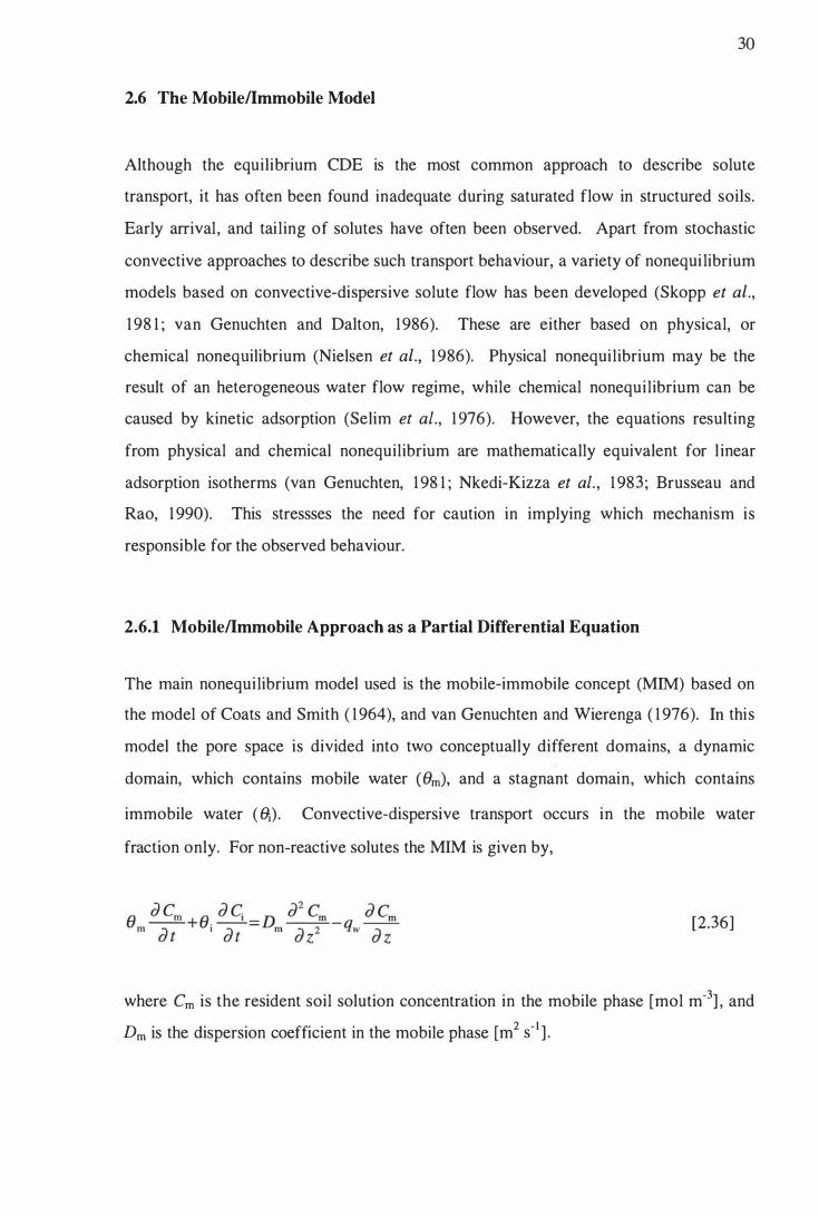
2.6 The Mobilellmmobile Model
Although the equilibrium CDE is the most common approach to describe solute
transport, it has often been found inadequate during saturated flow in structured soils.
Early arrival , and tail ing of solutes have often been observed. Apart from stochastic
convective approaches to describe such transport behaviour, a variety of nonequi librium
models based on convective-dispersive solute flow has been developed (Skopp et aI.,
1 98 1 ; van Genuchten and Dalton, 1986). These are either based on physical, or
chemical non equilibrium (Nielsen et aI., 1 986). Physical nonequilibrium may be the
result of an heterogeneous water flow regime, while chemical nonequilibrium can be
caused by kinetic adsorption (Selim et ai., 1 976). However, the equations resulting
from physical and chemical nonequilibrium are mathematically equivalent for l inear
adsorption isotherms (van Genuchten, 1 98 1 ; Nkedi-Kizza et ai. , 1 983; Brusseau and
Rao, 1 990). This stressses the need for caution in implying which mechanism is
responsible for the observed behaviour.
2.6.1 Mobilellmmobile Approach as a Partial Differential Equation
The main nonequilibrium model used is the mobile-immobile concept (MIM) based on
the model of Coats and Smith ( 1 964), and van Genuchten and Wierenga ( 1 976). In this
model the pore space is divided into two conceptually different domains, a dynamic
domain, which contains mobile water (8m), and a stagnant domain, which contains
immobile water ( �). Convective-dispersive transport occurs in the mobile water
fraction only. For non-reactive solutes the MIM is given by,
[2.36]
where em is the resident soil solution concentration in the mobile phase [mol m-3] , and
Dm is the dispersion coefficient in the mobile phase [m2 S- I ] .

3 1
Solute transport between the mobile and immobile domain is assumed to be diffusion
controlled, and described by a first order equation (van Genuchten and Wierenga, 1 976),
d C ( ) e· -' =a C -C , d t m ' [2.37]
where the subscripts m and i denote the mass in the mobile and immobile domain, and a
is the diffusional transfer coefficient for solute exchange between mobile and immobile
regions (s· ' ) .
2.6.2 Mobilellmmobile Approach as a Transfer Function
Alternatively the mobile/immobile concept can be presented as a transfer function. This
is discussed in detail by Sposito et al. ( 1 986) . They obtained the probability density
function of the MIM by numerical inversion of the Laplace-transformed pdf. The
effects of convection, dispersion, mobile/immobile water fractions, and mass transfer
coefficient on the shape of the travel time pdf were demonstrated. Also given were the
mean and variance of the solute travel time for the mobilelimmobile concept. The mean
solute travel time is the same as for the CDE, and the variance also growths l inearly
with travel distance. However the variance is influenced by the immobile domain, and
increases with an increase in the immobile water fraction, or a decreasing transfer
coefficient.
2.6.3 Critique on the Mobile!lmmobile Approach
The mobile/immobile concept of van Genuchten and Wierenga ( 1 976) has shown some
improvements over the CDE in describing the frequently observed early breakthrough
and tailing, for both repacked and undisturbed soil columns (Rao et aI., 1 980; Nkedi
Kizza et aI., 1 983; Seyfried and Rao, 1 987; De Smedt and Wierenga, 1 984; Vanclooster
et al. , 1 993). At a statistical-fitting level, this is however not surprising as the
mobile/immobile concept contains two more fitting parameters. As Jury et al. ( 1 99 1 )
demonstrated, by varying en/e, a, or the mobile dispersion coefficient Dm, various

32
shapes of BTC's can be obtained. The drawback of the model is that none of these
parameters is directly measurable, without making some assumption about the other
parameters . For example, Clothier et al. ( 1 992) recently proposed the disc permeameter
technique for determining the immobile water fraction, after dispersive effects had faded
away. However, they assumed that a was negligible. Jaynes et al. ( 1 995) on the other
hand considered that hydrodynamic dispersion was negligible, and thereby determined
a. It therefore seems more applicable to use the much simpler classical CDE, in which
the effects of matrix diffusion are lumped into the hydrodynamic dispersion coefficient
(Valocchi, 1 985).
Another point of dispute is the relationship between 0. and the pore water velocity v (De
Smedt et ai., 1 986; Nkedi-Kizza et at. , 1 983, van Genuchten and Wierenga, 1 977;
Kutflek and Nielsen, 1 994) . The fraction of the immobile water can either be
considered constant, or assumed to depend on the total water content. A constant
immobile water fraction can be assumed if the soil consists of distinct aggregates
(Zurmiihl and Durner, 1 996).
Although the mobile/immobile concept of van Genuchten and Wierenga ( 1 976) has
often been found successful in describing solute transport through structured soils, the
question remains whether this model is appropriate. Originally developed to describe
preferential flow and asymmetric BTC's , the concept is not based on clearly definable
physical processes. Furthermore, for reactive solutes, the mobilelimmobile model is not
the only conceptual model capable of describing asymmetric BTC's . The use of
nonlinear isotherms performs equally well in describing these observed phenomena.
This will be discussed in section 2.8. It would seem more useful to describe preferential
flow in terms of the transfer function approach, or the classical CDE with some
assumptions as to how the parameters change with flow rate and perhaps with depth.

33
2.6.4 The Link Between the Mobilellmmobile Approach and Bolt's Approach
Bolt ( 1 982) suggested an approximate relationship between the mobile/immobile
exchange length Lrnim and other parameters of the MIM is,
L . =(�)2 qw mlm e a ' [2.38]
The val idity of eq. [2.38] was tested numerically, and simulations are shown in Fig. 2.4
for two different column lengths of 300 and 500 mm, and LD = 50 mm, Ldis = 10 mm,
and Lmim = 40 mm. Assuming that e = 0.5, � = 0.25, and qw = 5 mm h- 1 , the value for a is found with eq. [2.38] to be 0.03 h- 1 • Note that LD in the CDE is the dispersivity A, and
that Ldis in the MIM is the dispersivity in the mobile phase Am. The agreement between
the predictions based on the two different models, and using the approach of Bolt is
good. However the major limitation of the MIM remains the inability to measure the
parameters � and a independently, and that different combinations of � and a can give
the same value of Lmim, and the same macroscopic solute behaviour.
o () ....... 0 .5
Lo= 50 m m Lm1m= 1 0 m m Ldls= 4 0 m m e = 0.5 m 3m ·3
ej= 0.25 m 3m ·1
qw= 5 m m h·1
IX = 0 .03 h·1
- C D E - - M IM
0.0 +--IO....---r----�----_+ o 1 2
L iqu id-f i l led p o re vo lu m es 3
Fig. 2.4. Comparison between simulations using the CDE and MIM, based on the approach of Bolt
( 1 982).

34
2. 7 Layer and Mixing Cell Models
A simple and useful approach for describing solute transport is the use of layer or
mixing cel l models, where the soil profile is divided into a number of horizontal layers
or cells. The incoming water and solutes are usually assumed to mix instantaneously and
completely with water and solutes already present in each cell during each time step.
Such models have been used to study both the transport of non-reactive and reactive
solutes (van Ommen, 1 985; Bajracharya and Barry, 1 993). Van der Ploeg et ai. ( 1 995b)
recently proposed a mixing cell model, which can be considered as a simplified version
of the CDE. They compared predictions using analytical solutions of the CDE with
their approach. They found good agreement for both flux and resident concentrations,
provided that the Peelet number P > 6, where P is defined as L / A. Dispersivities in
field soils commonly range from 1 - 200 mm (White, 1 985b). So in the case of a highly
dispersive soil with a A of 200 mm, the mixing cell model should only be used for
depths � 1 .2 m.
Apart from being computationally very simple, this mixing cell model has the advantage
that nonuniform initial solute distributions in the soil, and even transformation processes
(van der Ploeg et aI., 1 995a) can be easily included. Under these conditions, analytical
solutions for the CDE are not readily available.
2.8 Reactive Solutes
So far, discussion has centered on solutes which do not react with the soil matrix . Many
chemicals of agricultural or environmental interest are, however, attracted to soil
mineral or organic surfaces. This exchange critically controls the depths and pattern of
leaching. Two different types of exchange on the soil matrix have to be considered, a
constant, and a variable surface charge. While the constant surface charge is
independent of the solution concentration, the variable surface charge is determined by
the nature of the adsorbed ions, the concentrations of the ions in solution, and the pH of
the soil solution (Parfitt, 1 980; Bolan et ai., 1 986). Both anions and cations are to
varying degrees subject to adsorption and exchange reactions on the soil matrix.

35
Nitrate, chloride, bromide and tritium are usually considered to be non-reactive solutes.
However adsorption or exclusion of these solutes has also been observed to some
extent, depending on the chemical properties of the soil (Biggar and Nielsen, 1 962,
Krupp et aI. , 1 972).
In this section adsorption reactions onto the soil matrix are described by different
processes, and their effect on solute transport is discussed. The basic CDE presented
above [eq. 2.24] is modified to include adsorption isotherms, or exchange reactions.
2.8.1 Solute Adsorption
The total amount of solute in the soil M [mol m-3] is assumed to be partitioned into two
phases, the concentration on the adsorber Ss [mol kg- I ] and the concentration in the soil
solution Cr. Thus,
[2.39]
where Ph is the soil bulk density [kg m-3] . The relationship between the concentration
on the exchanger, and that in the soil solution at equilibrium is called an adsorption
isotherm. Generally, exchange reactions are assumed to be instantaneous, and
equilibrium is assumed between the soil solution concentration and the exchanger.
Including the concentration on the adsorber into the CDE results in,
[2.40]
Adsorption of solutes onto the soil matrix has been described in different ways. One of
the main approaches is the use of isotherms SsCC), which can be linear or of any other
functional form. A comprehensive review of adsorption isotherms is presented by
Helfferich ( 1 962) . One of the most commonly used is the Freundlich equation (Nielsen
et al. , 1 98 1 ),

36
[2.4 1 ]
where Kd is the distribution coefficient [m3 kg- I ] , and n is a constant which can be
obtained from isotherm data. The distribution coefficient is generally assumed constant.
However in some soils, Kd has been found to be dependent on the ionic strength of the
soil solution (Parfitt, 1 980, Bolan et ai. , 1 986). An example of such a soil is given in
Chapter 5 .
When the above adsorption isotherm is inserted into the CDE, it follows that,
R d Cr = D d 2 Cr _ v d Cr
d t S d Z 2 d Z [2.42]
where the dimensionless retardation factor R describes the velocity of a solute front or
pulse relative to the velocity of an non-reactive solute. From [2.40] and [2.42] ,
If eq. [2.43] is valid, it follows that,
C 0-1 R= l +npb Kd -r -e
or for l inear adsorption (n = 1 ),
[2.43]
[2.44]
[2.45]
For solutes which are adsorbed, Kd is positive, resulting in R > 1 . The effect of
adsorption is then to hold, or retard the rate of solute movement by the factor R.
Dispersion is reduced by the same factor. This means that the adsorbed solute will take
R times as long as a non-adsorbed solute to travel a given distance. When solutes are

37
subjected to anion exclusion Kd is negative, resulting in R < 1 . This then leads to
accelerated leaching of the solute.
The assumption of exchange equilibrium has sometimes resulted in an overestimation of
the amount of adsorption occurring during miscible displacement (Davidson and Chang,
1 972). As a result, kinetic adsorption models, where the amount of solute sorption is a
function of contact time (Lapidus and Amundson, 1952), and two-site linear adsorption
models (Selim et ai. , 1 976; Cameron and Klute, 1 977) have been developed. In the
two- site l inear adsorption model, the sorption sites are classified into two types, to one
of them sorption is assumed instantaneous, and to the other one sorption is assumed
time-dependent. However it is beyond the scope of this review to discuss these models.
2.8.2 Cation Transport
Retention of cations during transport through soils has been described using two
different approaches. One of them is the use of an adsorption equation, e.g. the
Freundlich equation [Eq. 2.4 1 ] . Application of this equation to cation exchange in soils
does not always, however, take into account competition between cationic species.
Another approach is to describe the interaction between the ions in the soil solution and
on the exchanger as a reversible and instantaneous exchange reaction. This is then
incorporated into the transport model (Robbins et al., 1 980). Adsorption of a cation
then also depends on other cation species in the soil solution. In a system with cation
species Ca2+, Mg2+, K+, and Na+, the total amount of adsorbed cations can be expressed
as,
[2.46]
where X denotes the charge concentration of adsorbed cations [mole kg- I ] and the
subscripts represent calcium, magnesium, potassium, and sodium. Although the cation
exchange capacity (CEC) of a soil often depends on the pH, and the ionic strength of the
soil solution, we first consider here a constant CEC. An example of variable CEC is

38
given in Chapter 6. Furthermore the discussion here will be limited to a description of
binary systems, involving either homovalent or heterovalent exchange.
Since it is assumed that cation exchange reactions are instantaneous and reversible,
equilibrium equations can be used to describe the relationship between cation species in
the soil solution and on the exchanger. A number of different equilibrium equations
have been proposed, and are reviewed by Bolt ( 1 967) and Bohn et al. ( 1 985). The most
commonly used equations are probably the mass action, Kerr, Vanselow or Gapon
equations. The main difference between these equations is in the treatment of the
activities of the involved cations. Firstly we consider cation exchange involving two
cation species A and B of the same valence, and with similar activity. If we assume that
the concentrations and activities for both the solution and the adsorbed phase are
directly proportional, then all the above equilibrium equations reduce to (Bohn et al.,
1 985),
K = CA XB A-B C X B A
[2.47]
where KA-B is the selectivity coefficient, and XA and XB are the charge concentrations of
adsorbed cations A and B [mole kg- I ] . The selectivity coefficient is generally assumed to
be constant (Freeze and Cherry, 1 979), but approaches with varying selectivity
coefficients have also been used, where KA-B is a function of the fractional coverage on
the exchanger phase (Mansell et ai., 1 988). The selectivity coefficient can be
determined experimentally by measuring the equilibrium ionic composition of several
soil solution systems having different exchangeable cation compositions.
Since the cation exchange capacity is assumed constant, it fol lows for a homovalent
system that,
[2.48]

39
where KA-B is the selectivity coefficient, XCEC is the cation exchange capacity of the soil
solids [mole kg- I ] , and CT the total solution concentration [mole r l ] , which for a solution
containing only cation species A and B is given by,
[2 .49]
Retardation for cation transport, assuming a constant CT is then given by (Selim et ai. , 1 987),
R= 1 + Pb XCEC ___ K-=A---!B'--_--;:;-e e, ( 1 + (KA_ , _ 1 )�)
2 [2.50]
Furthermore if nonpreferential exchange between cation species A and B is assumed
(KA-B = 1 ) , the above equation simplifies to
<Xl X
0.088 +-_---" __ ...1..-_--'-__ ""--_..,.."...
0.066
o 0.044 ...
x
0.022
0.000 -i"'-'--"'--"T'"""---r---r---t-0.000 0.005 0.0 1 0 0.0 1 5 0.020 0.025 CAor C8
[2.5 1 ]
Fig. 2.5 Exchange isothenns for a homo valent system with cation species A and B for various values of
the selectivity coefficient KA-B.

< c :2 «l 0
.2 E 0 E-O
40
Exchange isotherms for various values of KA-B are plotted in Fig. 2.5 for a homovalent
system. It can be seen that for KA-B 1= 1 the isotherm is nonlinear. For a KA-B < 1 the
isotherm becomes favourable for cation species A (convex upward), and unfavourable for cation species B (concave upwards).
The effect of the two different types of isotherms, unfavourable or favourable, on the
shape of the breakthrough curve is shown in Fig. 2 .6a and 2.6b. In all cases the
simulations were carried out for a Peelet number of 1 0, KA-B values of 0.3, 0.7 and 1 , a
CEC value of 0.05 mole kg- I , a Ph of 1 .4 Mg m-3, and a () of 0.4 m3 m-3 .
1 0
5
o
(a)
1 0 2 0 Liq u id -f i l led po re vo lu m e s
o E-o
30
1 0 �------�------���_�_�-�+ (b) . . . .
o +-,-:...,Il;"�-----r-------""--------+ o 1 0 20
L iqu id -f i l led p o re vo lu m es 30
Fig. 2.6 BTC's for a homovalent system with cation species A and B for various values of KA-B for (It) an
unfavourable isotherm, and (ta) a favourable isotherm.
It is evident from Fig. 2.6 that a nonlinear isotherm causes a change in the spreading of the solute front, similar in effect to hydrodynamic dispersion. Two totally different
processes can hence have a similar effect on the pattern of solute transport and the shape of the BTC. For an unfavourable isotherm, the spreading increases with increasing nonlinearity in the isotherm. Whereas for a favourable isotherm the spreading decreases
with increasing nonlinearity. In the case of an unfavourable isotherm (Fig. 2.60) adsorption is relatively low at low concentrations, resulting in an earlier concentration rise. With increasing concentration the slope of the isotherm increases, resulting in a
tailing effect. For a favourable exchange isotherm (Fig. 2.6q), the opposite effect

4 1
occurs, with high adsorption at low concentrations, resulting in a delayed concentration
rise. The decrease in the isotherm slope at higher concentrations then sharpens the BTC.
The most-commonly used equilibrium equation to describe cation exchange for
heterovalent systems under practical concentration ranges, is the Gapon equation (Bohn et ai. , 1 985),
[2.52]
where the subscripts M and D denote monovalent and divalent cation species, and KM-D
is the selectivity for the monovalent-divalent system [(mol m-3) 1/2] .
Equilibrium equations (eqs. [2.47] and [2.52], i n conjunction with eq. [2.46] can be
directly incorporated into the CDE. This is described in detail in Appendix A.
Exchange equations (eq. [2.48] to [2.5 1 ]) in conjunction with the CDE have been used by numerous investigators to describe cation transport through repacked aggregated soil (Selim et ai., 1 987; Schulin et ai., 1 989). Predictions based on this have been found to be relatively good. However use of the mobilelimmobile concept has often resulted in improved predictions of the observed tailing of breakthrough curves (Selim et ai. ,
1 987). Nonequilibrium in cation transport is, however, as Selim et al. ( 1 987) pointed out "inconsistent with tritium and 36CI transport data which indicated local equil ibrium". Hence the use of the mobile/immobile concept to describe cation transport seems sometimes to be more pragmatic than fundamentally sound.
It should also be kept in mind that the shape of the isotherm affects the shape of the
BTC, as was shown in Fig. 2.6. Nonlinear isotherms can result in increased dispersion and tailing. However tailing can also be simulated by using the MIM with l inear isotherms, and by adjusting the ratio between the mobile and the immobile fraction. Although models based on physical or chemical non equilibrium have often resulted in
improved predictions of both anion and cation movement, it seems that these models are

42
too complicated to be useful as a predictive tool. They require a large number of
parameters, which so far cannot be measured independently. Different set of parameters can predict the same solute transport behaviour.
2.9 Boundary Conditions and Solutions for the Convection-Dispersion Equation
2.9.1 Flux and Resident Concentrations
The various formulations of the CDE can sometimes be solved analytically. They can
always be crunched numerically. Both analytical and numerical simulations of solute transport require the specification of initial and boundary conditions. The use of the appropriate boundary condition to describe the method of solute application to the soil is
critical for the parameter estimation. The choice of solution depends on the type of
solute concentration measured, either the flux or the resident concentration (Fig. 2.2).
Flux concentrations (Cf) are obtained from measurements of effluent from a soil
column, or a lysimeter. Resident concentrations (Cr) are obtained by sectioning soil
cores and extracting the soil solution, or by in situ electrical resistance measurements of the soil, such as by Time Domain Reflectometry.
c o
-� -c Q) (,) c o <.)
o 1 2 L iq u id -f i l le d p o re v o lu m e s
3
Fig. 2.7 Flux (solid lines) and resident concentrations (broken l ines) for two different Pec\et numbers.

43
The importance of distinguishing between these two types of concentrations when describing convective-dispersive transport was emphasised by Kreft and Zuber ( 1 978), and Parker and van Genuchten ( 1 984), and is shown in Fig. 2.7. In the simulation a solute pulse in the flux concentration was applied to the soil surface, and the
concentration at a depth 1 was simulated as either the flux concentration (solid l ines), or
the resident concentrations (broken l ine). Two different simulations are shown, with
Peclet numbers (P) of 6 and 30, where P is defined as l / A.. The difference between the
two predictions increases with increasing dispersivity (A.), as is apparent from eq. [2.26] .
Misinterpreting the resident concentration as a flux concentration can result in an
overestimation of both A. and the retardation factor R.
2.9.2 Boundary and Initial Conditions
The analytical solutions of the convection dispersion equation for a number of boundary
conditions are given by van Genuchten and Alves ( 1 982). Here only the solutions for
the boundary conditions pertinent to this study are described.
The most-common initial condition is that the initial concentration in the soil is zero, given by,
for t = 0 and 0 < z � l . [2.53]
where Cr is the volume averaged or resident concentration, Cf the flux-averaged
concentration, t the time, z the depth [m] and l the length of the column [m] . In certain applications, solutes are initially present in the soil , with the initial concentration of them varying with depth. In this case the CDE requires numerical solution.
The lower-boundary condition for the outlet of finite length columns recommended by Parker and van Genuchten ( 1 984) is that applicable for a semi-infinite domain, that is
aa�r (oo, t) = 0 . [2.54]

44
This boundary condition ignores any effects due to the finite length of the column.
However as the exit reservoir is not in contact with the l iquid phase inside the column, diffusion and dispersion at the outlet end can be neglected. So, this solution can also be
used for finite systems, where 0 � x �l (Parker and van Genuchten, 1 984) .
Much discussion can be found in the literature about the inlet boundary condition most
appropriate. Under steady-state water flow conditions, two different input functions are commonly considered, a first- and a third-type condition. The first-type condition defines the solute concentration at the soil surface. For a constant surface concentration
Co it is,
for z = 0 and t � 0 . [2.55]
The third-type or flux boundary condition defines the solute flux density at the upper
surface. For a constant flux density it is,
for z = O, t � o [2.56]
where Co is the input concentration, Cr the resident concentration, and Ds is the hydrodynamic dispersion coefficient. This third-type condition assumes that molecular
diffusion and dispersion above the soil are negligible, which can lead to differences between Co and Cr at z = o. Hence the discontinuity in the concentration at the inlet end (Parlange et al., 1 985) increases with the dispersivity. This third-type boundary
condition is generally preferred as it more closely approximates the experimental conditions usually imposed. It is recommended by van Genuchten and Parker ( 1 984) for
effectively semi-infinite systems, or finite systems of length 1, when P � 5 . This surface
boundary condition does not allow solute to diffuse upwards, which means that the symmetry of the diffusion process is broken. The centre of a solute pulse consequently moves downward more quickly and spreads out more slowly than it would in an infinite
medium. In very short columns, with a low Peclet number, it implies an early
breakthrough similar to that induced by preferential flow. This is however an artifact of
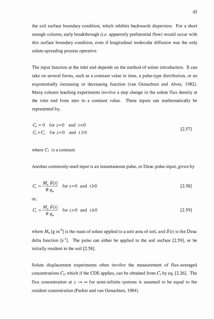
45
the soil surface boundary condition, which inhibits backwards dispersion. For a short
enough column, early breakthrough (i.e. apparently preferential flow) would occur with this surface boundary condition, even if longitudinal molecular diffusion was the only solute-spreading process operative.
The input function at the inlet end depends on the method of solute introduction. It can
take on several forms, such as a constant value in time, a pulse-type distribution, or an
exponential ly increasing or decreasing function (van Genuchten and Alves, 1 982).
Many column leaching experiments involve a step change in the solute flux density at the inlet end from zero to a constant value. These inputs can mathematically be
represented by,
Cf = 0 for z = O and t <O Cf = C1 for z = O and t � O
where C1 i s a constant.
[2.57]
Another commonly-used input is an instantaneous pulse, or Dirac pulse-input, given by
for z = O and t �O
or,
Cr -_ Mo 8 (t) f 0 d 0 or z = an t � e qw
[2.58]
[2.59]
where Mo [g m-2] is the mass of solute applied to a unit area of soil , and 8 (t) is the Dirac
delta function [S- I ] . The pulse can either be applied to the soil surface [2.59] , or be initially resident in the soil [2.58].
Solute displacement experiments often involve the measurement of flux-averaged concentrations Cf, which if the CDE applies, can be obtained from Cr by eq. [2.26] . The
flux concentration at z -7 00 for semi-infinite systems is assumed to be equal to the
resident concentration (Parker and van Genuchten, 1 984) .

46
2.9.3 Analytical Solutions
Analytical solutions have been widely used for interpretation of laboratory experiments.
Although analytical solutions are limited to conditions of steady-state water flow, uniform water content, l inear processes, and restricted initial and boundary conditions,
valuable information can be gained by their use. A number of analytical solutions for different boundary conditions for one-dimensional solute transport are given by van
Genuchten and Alves ( 1 982).
The solution for the resident concentration following a step change in the input flux
concentration [ego 2.57] is given by (van Genuchten and Wierenga, 1 986),
( /c - 1 rf [ z - vt ] ( V2 t ) [ (Z - vt)2 ] T I) - - e c + -- exp
2 2 .JDs t n Ds 4 DJ
1 ( v Z v2 t ) (v z ) [ z + v t 1 - - 1 + - + - exp - erfc 2 Ds Ds Ds 2.JDs t
where erfc is the complementary error function.
[2.60]
The resident concentration following a pulse input in the flux concentration [ego 2.59] is (Kreft and Zuber, 1 978),
[2.6 1 ]
The solutions for the flux-averaged concentration (Cf) can be derived directly from the solutions of the resident concentrations by recalling the relationship between the flux
averaged concentration and the volume-averaged concentration [ego 2.26] .

47
The solution for the flux concentration following a step change in input is given by
(Kirkham and Powers, 1 97 1 ),
�Cf(Z, t) = .!..[erfc. ( z - v t J + exp (_vzJ erfc ( z + v t Jl Co 2 2 �Ds t Ds 2 �D. t
[2.62]
and for a pulse input the solution is (Kreft and Zuber, 1 978),
[2.63]
Equations [2.60-2.63] are commonly used analytical solutions of the CDE. These are
only valid for the assumptions made in the model, and for the boundary conditions
described above.
2.9.4 Numerical Solutions
In situations that mimic the conditions often found in either the laboratory or field, the
CDE can only be solved by numerical procedures. Numerical solutions are needed when transient water flow or nonlinear adsorption processes occur. They also offer more flexibility in the initial and boundary conditions and with modern day computers and
software, their solution is not too difficult. To solve the CDE numerically a number of different approaches can be used. In all of them, the soil profile is divided into notional
compartments each & thick, and the time period into notional time steps Ilt long. For
each compartment initial conditions are specified, i. e. for compartmen(�n ';1t the � th time l.
step, the water content is e nj , the solute concentration Cn j, and the solute mass Mnj, where the subscripts n and j refer to depth and time. In the numerical schemes used here, a flux type boundary condition [eq. 2.56] is used to define the boundary condition
at the soil surface. A zero concentration gradient [eq. 2 .54] is assumed deep in the soil

48
profile. In the numerical procedure this is approximated by adding extra notional layers. The numerical grid is shown in Fig. 2.8.
n- l n n+l
nl
nIl
J j+l j+2
• known values
[QJ unknown values
Fig. 2 .8 Numerical grid where the depth is downwards and time marches to the right.
The main numerical procedures used in this study are described in Appendix A, and
examples of computer programs are given in Appendix B .

49
2. 10 Classification of Solute Transport Models
In the above sections, various approaches to the modell ing of solute transport through the soil have been discussed. These, and several other approaches, are discussed and
classified in reviews by Addiscott and Wagenet ( 1 985), Brusseau and Rao ( 1 990), and
Kutflek and Nielsen ( 1994). Solute transport models are commonly grouped under two
broad headings: deterministic or process models, and stochastic models. In
deterministic models, such as the convection dispersion equation (CDE), it is assumed
that a given set of events leads to a uniquely-definable outcome. Conversely, in stochastic approaches, the parameters are treated as random variables with a certain probability function (pdf) assigned to them. The value of random variables can be
different at each point in the soi l . Random variables can also be a function of time.
Solute transport behaviour is then treated as a random phenomenon, which means that at any location a number of outcomes can be predicted by the model. Stochastic models include the stochastic version of the CDE (Bresler and Dagan, 1 979), Monte Carlo
simulation approaches (Amoozegar-Fard et al., 1 982), and the stochastic convective stream tube model of Jury and Roth ( 1 990).
On closer examination, however, the above classification seems somewhat artificial, as "stochastic" models do not usually treat solute transport behaviour at either the laboratory or the field scale as a random phenomenon. Although the stochasticconvective model of Jury ( 1 982) has apparently been developed with the idea of randomness, the approach would only be stochastic if a heterogeneous field were
visualised as consisting of numerous independent "stream-tubes" in which the transport
properties, such as the pore water velocity and the dispersion, are constant in each column but vary randomly between "stream-tubes". In practice the randomness is
assumed to occur at a smaller scale, and measurements are not made of individual "stream-tubes". The measured concentration in a certain volume of soil at a certain depth is used to infer the distribution of travel times through a number of notional independent and randomly-distributed pathways or stream tubes, thereby giving for an
REV an expected value for the solute travel time and its variance. If these stream tubes
are thought of as being macropores, solute concentrations are not really sampled at random. Instead the pdf is assumed to be the same for every REV in the soil , and the

50
expected value and its variance are constants. Furthermore the travel time distribution, characterised by the probability density function, is assumed to be characteristic for a
certain soil, which means that at the scale at which measurements are made, the
outcome is not uncertain.
In other classification schemes, models have been grouped into mechanistic and nonmechanistic models. Mechanistic models are believed to be based on the physical processes involved. However the fact that a mechanistic model fits a given data set does
not necessari ly prove the validity of certain physical mechanisms, but only shows that
the operation of those is consistent with the data. Mechanistic models imply that
predictions of solute concentrations can be made for all depths. Thus mechanistic models include not only the CDE, but also the stochastic convective stream tube model
of Jury and Roth ( 1 990). However the issue of mechanistic or non-mechanistic is quite
confusing. For example, Jury ( 1 983) states "The transfer function model has no mechanisms . . . ", and a few pages later the fol lowing contradictory statement is given: . . "that convective models such as the transfer function modeL.". Strictly speaking the
only non-mechanistic models would be "black box" approaches, such as the original transfer function model of Jury ( 1 982), applicable to only one depth. However as these
models cannot be used to predict solute transport under conditions different from those used for cal ibration, such models would seem of l imited util ity. If we want to use models as a predictive tool, we have to open the "lid" of the "black box".
A system is a big black box Of which we can't unlock the locks,
And all we can find out about Is what goes in and what comes out.
Perceiving input-output pairs, Related by parameters,
Permits us, sometimes, to relate An input, output, and a state.
If this relation is good and stable Then to predict we may be able,
But if this fails us - heaven forbid! We' l l be compelled to force the lid!
Kenneth Boulding

5 1
Additionally, models have been classified with reference to their purpose: research or
management oriented. Whereas research-based models aim at a complete understanding of the processes, management-oriented models are thought of as being mainly useful as guides to the best management of soils. However this separation also seems arbitrary, as models are only useful if solute transport under various conditions can be predicted. This seems only be possible if the processes involved are reasonably described. A
proper understanding of solute transport does not negate the use of simplified models, but stresses the need to test the validity of these models under various conditions.
In conclusion, clear-cut model classification is difficult. It can give misleading impressions about the differences between models, such as being "stochastic" or "non
mechanistic". In fact it seems that classifying models has increased rather than decreased the confusion as to how they are different. Classification using fuzzy-set
logic would seem more appropriate.
2. 1 1 Conclusions
This chapter on solute transport theory and transport models shows that models based on quite different physical and chemical assumptions can result in identical predictions
of solute transport.
• The comparison of predicted and observed breakthrough curves can therefore not be considered as a test for the unique validity of any mathematical model or mechanistic description.
• The approach of Bolt was used to demonstrate the relationship between the
convection dispersion equation and the mobile/immobile approach.
• Although the MIM is conceptual ly pleasing, it seems of l imited applicability. This is because the same predictions can be made using the simpler CDE, and so far it is not possible to independently estimate the required parameters in the MIM.
Consequently, the parameters are generally estimated from BTC's by fitting

52
procedures. But several sets of parameters usually fit BTC data equally well , but
give different predictions for solute transport under different conditions or to different depths. Also it is questionable, if the model parameters obtained by fitting
have any physical meaning.
• Some approaches assume well-defined soil geometry to estimate the parameters of the MIM. It seems however that instead of simplifying the soil by assuming a well
defined structure (e.g. spherical aggregates), a simplified model such as the CDE
should be used, provided it performs satisfactorily.
• The CDE can be used for transient water flow, and it can incorporate exchange reactions and production or decay of solutes. The performance of the CDE will therefore be the focus of this study.

Chapter 3
3. The Theory of Time Domain Reflectometry For Measuring
Soil Water Content and Solute Concentration
3. 1 Introduction
53
Monitoring and predicting solute transport at the field-scale is important, and thi s has
been emphasized by several authors (Jury, 1 982; Butters and Jury, 1 989). Kutflek and
Nielsen ( 1 994) concluded that " . . . without properly taken field data all our effort is futile". To characterize adequately a site, and to obtain a better understanding of water and solute transport at the field-scale, large numbers of measurements are needed, in
part because of the high spatial and temporal variabil ity. The traditional technique for measuring the soi l ' s water content involves oven-drying of a soil sample, and
determining the weight loss (Gardner, 1 986). This so-called 'gravimetric ' technique is
not only time consuming, but more importantly, it is destructive and hence not suitable for regular in situ monitoring of soil water content. An alternative method, and up until recently the most-widely used method for in situ measurement of soil water content is the neutron probe (Jury et aI. , 1 99 1 ) . This method also has many disadvantages, including the attendant radiation hazard, the inability to measure close to the soil surface, and the need for soil specific calibration. There has thankfully been a recent
technological advance: Time Domain Reflectometry (TDR).
The traditional method for the determination of the solute resident concentration in the soil is solution extraction from soil samples. However, as with gravimetric water content measurements, this method is also time consuming and destructive. Solute concentration can also be measured using suction cups, but problems include the
adsorption of ions by the ceramic material . Furthermore suction cups may only sample
water from the mobile regions of the soil water domain . Water in the immobile region might not be drawn into the samplers (van Genuchten and Wierenga, 1 977). So there is
the uncertainty of whether the sample concentrations represent a resident or a flux concentration (Elrick et aI. , 1 993, Kachanoski et al., 1 994). Until very recently

54
simultaneous measurements of water content and solute concentration have been difficult to make.
Over the last decade, the new technique of time domain reflectometry (TDR) has been
proposed to monitor not only the soil ' s water content, but also the electrical conductivity of the soil solution. The technique has proved successful, provided that appropriate
calibrations are available (Topp and Davis, 1 985; Dasberg and Dalton, 1 985;
Heimovaara, 1 993). TDR for measuring soil water content, e, has now become a well
accepted method (Topp and Davis, 1 985, Zegelin et ai., 1 989, Dalton, 1 992) and
potentially the electrolyte concentration in the soil solution. However, despite numerous
applications of this technique to measure the bulk soil electrical conductivity (a), the
relationship between a and the solute concentration of the soil solution is not yet
completely understood (Yanuka et ai., 1 988). However, with the potential of thi s dual
capacity, TDR offers great scope for monitoring solute transport. Researchers are now
using this method increasingly because it is the easiest and most reliable way to measure
both e and a in situ.
Further advantages of TDR are its good spatial and temporal resolution, and its ability to measure very close to the soil surface (Hook et ai. , 1 992), plus the ability to measure the
total resident electrolyte concentration in both the mobile and immobile water regions. Multiplexers can be used to automate the measurements (Heimovaara and Bouten, 1 990;
Baker and Allmaras, 1 990; Herkelrath et ai., 1 99 1 ) . The ability of automating TDR for
the measurement of e and a makes TDR a potentially valuable tool for monitoring water
and solute movement, allowing a large number of measurements to be made (Heimovaara and Bouten, 1 990) to assess variations in space and time. A possible disadvantage of TDR for measuring solute transport is its l imitation to detecting only those solutes that alter the electrical conductivity.
This chapter gives a general introduction to the principles and practice of TDR to
measure both the soi l ' s water content and solute resident concentration. In the following chapter, cal ibration measurements from two different soils to determine both
the water content and the solute resident concentration are presented. These calibrations

55
are then used to assess the ability of TDR to monitor solute transport through repacked
and undisturbed soil columns. The TDR method is compared with traditional methods of monitoring solute transport.
3.2 The Measurement System
The TDR used here consists of a three-wire probe connected via a coaxial cable to a commercial cable tester ( 1 502 C Tektronix, Beaverton, OR). The coaxial cable consists
of an inner conductor and a metal shield, separated by a dielectric material. The
dielectric material is generally polyethylene, in which case the wave travels at 0.66 the
speed of l ight. This is the so-called 'velocity of propagation' , and the ratio we wil l later refer to as the relative velocity setting (vp). The cable tester is operated under computer control using special software developed by Steven Green of HortResearch (pers. comm.).
The cable tester sends out an electromagnetic wave, which travels down the coaxial cable, and enters the probe which is embedded in the soil . The core of the coaxial cable is connected to the centre-wire of the probe, and the shield to the outer two. The probe mimics a coaxial system, thereby obviating the need for an impedance matching balun (Zeglin et ai. , 1 989). A typical setup is shown in Fig. 3 . 1 . The electromagnetic wave consists of an electrical part and a magnetic part. For most soils in the determination of
the soil water content, the magnetic part is irrelevant. The electrical part of the
travelling wave is influenced strongly by the associated dielectric properties of the soil constituents, especially the water content. The fast-rise, step-shaped voltage pulse of these devices contains a spectrum of frequencies (Fellner-Feldegg, 1 969) in the high
MHz to GHz range (Topp et ai., 1 980) . The voltage pulse travels from the coaxial cable into the probe. At the end of the probe the signal is reflected. The travel time of the
wave along the transmission l ine is extremely short, usually in the range 1 to 1 00
nanoseconds, given the typical lengtb of probe length used in the soi l .

c:::J c:::J c:::J c:::J
Tectronix 1 502 C
0 0 0 0
Fig. 3 . 1 Schematic diagram of the TDR system.
56
The impedance is the total resistance of a conductor to AC current, and is measured in
[.0] . Any change in the impedance sensed along the line causes partial reflection of the
wave, which itself causes a change in voltage between the conductor and the shield.
Any reflected wave becomes superimposed upon the waves transmitted from the cable
tester. The change in voltage is detected by the TDR and then shown on the oscil loscope as the reflection coefficient (r). This reflection coefficient is the ratio of
the voltage reflected back to the receiver, divided by the voltage applied by the TDR unit. The TDR device measures the propagation and reflection of the pulse, as well as its attenuation. The entire curve can be simply called the trace.
In Fig. 3.2 is illustrated an idealized trace. The dielectric constant and the bulk soil electrical conductivity can be calculated from this wave form. Such measurements
provide the basis for calculating the volumetric water content around the probes, and the corresponding soil solution electrical conductivity of the soil solution.
The cable tester produces an electromagnetic wave and produces an increase in voltage between the conductor and shield equal to about 0.225 V. The wave then enters the coaxial cable at point A, and travels down the cable to the TDR probe at point B. At
this point, some of the voltage pulse is reflected back from the beginning of the probe.
The remainder of the pulse is transmitted. Any decrease in impedance at point B results

57
in a counter phase reflection, and can produce a drop in amplitude compared to the
launched voltage pulse. At point C, which corresponds to the end of the probe, the remainder of the transmitted voltage pulse is reflected, in phase, so that the total
amplitude becomes twice the transmitted voltage pulse, in the absence of any signal loss. On the way back to point B some of the reflected signal is transmitted through to point A, and the remainder is again reflected back towards point C. This continues until
the multiple reflections finally die away, and the final voltage level D is reached.
In summary, any increase in impedance along the cable, or the transmission l ine, results
in an increase in voltage, such as occurs at the end of the probe. Conversely, a decrease in impedance will results in a decrease in voltage, as occurs when the wave travels down the TDR probe.
V j� D � � - - -.---� A B
v· l n T
I V; Vr c
� I--
Fig. 3 .2 An idealized TDR voltage trace vs. time.
A : output of TDR B : reflection from probe beginning C : reflection from probe end D : final voltage level after multiple
reflections AB: coaxial cable travel time BC: TDR probe travel time T : travel time Vo : zero-reference voltage Vi : voltage of incident step Vr : voltage after reflection from probe
end Vf : final reflected voltage at very long
time
3.3 TDR for Measuring Soil Moisture Content
The TDR measurement technique was developed Fel lner-Feldegg ( 1 969), who used it to
measure the apparent dielectric constant (£) of l iquids in a coaxial wave guide. The use
of TDR for measuring the dielectric constant of soil was originally proposed by Davis and Chudobiak ( 1 975), and Topp et al. ( 1 980). The dielectric constant of soil depends
on the volume fractions of the soil constituents and their individual dielectric constants.

58
Representative values of £ are 80.36 for liquid water, 3-5 for soil minerals, 6-8 for
organic matter, and 1 for air, at a frequency of 1 GHz and a temperature of 200 C
(Weast, 1 965). Thus, the £ of a soil is dominated by the volumetric content of water
because of its high c. The dielectric constant consists of a real part, and an imaginary
part. The real part of the dielectric constant is a measure of the polarisability of the constituents, while the imaginary part represents the energy absorption by ionic conduction, or dielectric losses. The only polarisable molecules in soils tend only to be
water molecules. The relationship between £ and e developed by Topp et al. ( 1 980) has
now been widely adopted as a calibration standard for soils with low organic matter content.
The determination of the soil water content by TDR involves the measurement of the propagation velocity (ve) of the electromagnetic pulse as it travels along a waveguide, or
TDR probe, embedded in the soi l . The relationship between Ve and £ of a material is
given by (von Hippel, 1 954):
c [3. 1 ]
where tan 8 is the loss tangent, which is generally assumed to be « 1 (Topp et ai., 1 980).
Thus eq. [3. 1 ] can be written as,
-112 Ve = c £ [3 .2]
where c is the propagation of an electromagnetic wave in free space (viz. 3x 1 08 m s-\ and £ is the dielectric constant of the medium. As already noted, the dielectric constant
consists of a real part, and an imaginary part. If the electric loss in the soil is small , then the imaginary part can be neglected (Topp et at., 1 980) . Hence, only the only real part of the dielectric constant affects the wave velocity, or the pulse transit time in the probe. Over the frequency range 1 MHz to 1 GHz, the real part of the dielectric constant in soil

59
is not strongly dependent on frequency (Davis and Annan, 1 977). Thus, the dielectric
constant of the soil measured can be considered only a function of the soil ' constituents.
The propagation velocity in the soil can be obtained directly from TDR measurements. It is calculated from the time t [s] taken for the reflected signal to travel forth and back
along the probe, which corresponds to the interval Be shown in Fig. 3 .2. So,
[3.3]
where I t is the physical length of the probe [m] .
By combining Eq. [3.2] and [3.3] it is possible to eliminate Ve and to determine the dielectric constant of a medium from the measured travel time,
[3 .4]
In commercial TDR cable testers, the term c t12 is replaced by an apparent probe length Ia/vp which is obtained directly from the trace. Here vp is a fraction, being the relative velocity to the speed of l ight, which accounts for the specific dielectric of the coaxial cable. This vp value can either be set manually on the panel of the instrument, or it can
be changed under software control.
The volumetric water content of the soil can then be determined by calibration based on
a simple measurement of E. Different approaches have been proposed to relate E and 8.
Some employ mixing laws (Roth et al., 1 990b; Dirksen and Dasberg, 1 993), while others are empirical (Topp et aI. , 1 980). The empirical relationship found by Topp et al.
( 1 980) was initially claimed to be universal, and independent of soil texture, soil density
and salinity influences. For this reason it is often referred to as the 'universal relation' (Zegelin et al., 1 992). The relationship is :

60
e = -5.3 x 1 0-2 + 2.92 X 1 0-2 £ - 5.5 X 1 0-4 £2 + 4.3 X 1 0-6 £3 . [3.5]
This empirical relationship has been substantiated by other investigators (Dalton and van Genuchten, 1 986; Zeglin et al., 1 989). Roth et al. ( 1 992) found it appropriate for
mineral soils with absolute error in e of about 0.0 1 5 m3 m-3 . If higher accuracy is
required, individual calibrations were considered necessary. Since then, other
influences on the e-£ relation have also been studied. These include bulk density
(Ledieu et al. , 1 986), and soil temperature (Roth et al., 1 990b). For organic soils this
so-called 'universal ' relationship has often been found inappropriate. This might be due
to the higher amount of bound water associated with organic matter, as bound water has a lower dielectric constant, due to the restricted rotational freedom of the l iquid water
molecules.
An alternative to eq. [3.5] is, as noted before, the use of mixing models . Here £ is
obtained from the individual £ of the three soil components, the soil , the enclosed air,
and the volume fraction of water. Major constraints for the use of mixing models include the difficulty in determining the required constants, and the effect of bound
water. Empirical 8-£ relations were used in this study.
3.4 TDR for Measuring So/ute Concentration
Dalton et al. ( 1 984) first proposed the use of TDR for measurIng the electrical
conductivity (a) of the soil. They demonstrated that the attenuation of a voltage pulse
along the probe could be used to deduce a. This attenuation was used to infer the solute
resident concentration (Cr). Since then severa] different approaches have been
suggested for using the attenuation of the reflected signal to determine a, and they are
based on use of various values of the voltage at different points along the TDR-trace (Fig. 3 .2). However, so far it remains unresolved as to which of the alternative
expressions is the most appropriate for the calculation of (J.

6 1
Dalton et ai. ( 1 984) used the ratio of the signal amplitude from the start of the probe and
the voltage upon its first reflection from the probe, (Vr -VD1Vi, to find (j (Fig. 3.2).
According to electromagnetic field theory (Ramo and Whinnery, 1 958), the amplitude of a perfect reflection from the end of a transmission line embedded in an electrically
conductive medium with an attenuation coefficient ill, is diminished to
[3 .6]
where Vi is the voltage that enters the transmission line, and it is the length of the probe.
The attenuation 0) is given by:
60 n (j ill = 1 /2 £
and so it follows that:
(j = In r I [ £1/2 ( V - v ]]
1 20n i( V; .
[3 .7]
[3.8]
Later work (Topp et ai., 1 988) demonstrated that multiple reflections of the signal can occur. These multiple reflections are ignored in the approach of Dalton et ai. ( 1984).
By using the attenuation voltage at long times (Vf), Yanuka et al. ( 1 988) considered the effect of multiple reflections. They found,
[3 .9]
Zegelin et al. ( 1 989) adapted the method of thin-sample conductivity analysis originally proposed by Giese and Tiemann ( 1 975), and they were able to show good agreement
between values of (j measured with an AC conductivity bridge, and those measured by
TDR. They used the formulation,

62
[3. 1 0]
It is noted that all of the above formulations (eqs. [3 .8] , [3.9], [3 . 1 0]) require
simultaneous measurement of the dielectric constant to determine a value for (J.
Nadler et al. ( 1 99 1 ) proposed yet another method of determining (J, based on
measurement of an impedance of the TDR-probe (ZL [0]). To determine a value for ZL
they used the voltage reflection coefficient r, which is the ratio between the reflected
amplitude at long times and the incident signal amplitude. Thus here,
[3 . 1 1 ]
where Zo is the characteristic impedance of the cable [0] . The reflection coefficient can
be directly read from the screen of the TDR, thereby allowing an immediate calculation
of ZL. Nadler et al. ( 1 99 1 ) then converted ZL to (J using an equation identical to that of
Rhoades and van Schilfgaarde ( 1 976),
[3 . 1 2]
where (J25 is the bulk soil electrical conductivity at 25° C, KG is the probe-geometry
constant [mo l ] , and Ie is a temperature correction coefficient, appropriate for
temperatures other than 25° C (US Salinity Laboratory Staff 1954, Table 1 5). The
probe-geometry constant is influenced by the length, spacing, and the diameter of the
transmission lines. It can, however, be easily determined by immersing the TDR probe
into solutions of various known electrical conductivities and measuring the respective
impedances (Nadler et al., 1 99 1 ),
[3 . 1 3]

where aref is the electrical conductivity of a reference solution at 25° c.
Alternatively, ZL can be calculated using the respective voltages (Wraith et al., 1 993)
[3. 1 4]
The bulk soil electrical conductivity is then calculated using equation [3 . 1 2] .
63
The method of Nadler et al. ( 1 99 1 ) and Wraith et al. ( 1 993) for determining the
reflection coefficient from voltages after multiple reflections seems to provide a
practicable means for the determination of a, as it does not involve many parameters.
The TDR-measured electrical conductivity of the bulk soil is a function of the water
content, the pore-water electrical conductivity (aw) due to ionic species in the soil
solution, as well as the surface conductance (as). The latter is hopefully small compared
to aw (van Loon et ai., 1 99 1 ; Mualem and Friedman, 199 1 ). If the surface conductivity
can be disregarded, then the pore water electrical conductivity can be obtained from
simultaneous measurements of e and a, provided the relationship between a, e, and aw is known. Subsequently, the solute resident concentration (C) can then be calculated
from known relationships between aw and Cr, if the chemical composition of the soil
solution is also known. Different approaches can be found in the literature for obtaining
aw from measured values of a. Most of these are based on mixing laws, where the
determination of various soil parameters is necessary (Rhoades et al., 1 976; van Loon et al., 1 99 1 ). It remains difficult to obtain exact values of aw , due to the lack of
cal ibration constants, and the difficulties involved in their determinations. Rhoades et al. ( 1 976) suggested that the electrical conductivity of a soil can be approximated by:
[3. 1 5]

64
where 't' is an electrical tortuosity factor, which is depends on e. Rhoades et ai. ( 1 976)
proposed a simple empirical relationship between 't' and e given by,
't' = a e + b [3. 1 6]
where a and b are soil dependent constants. These constants must be found by
calibration.
Ward et al. ( 1 994) suggested two different methods to determine the a-Cr calibration.
The first was an indirect method, adopted from Kachanoski et al. ( 1 992), and performed
on column outflow experiments. This assumes that the final value of aw equals that of
the input solution. For a multitude of reasons (e.g. immobile water, exchange
reactions), this assumption need not always be valid. The second approach is a more
direct method, and requires separate experiments, in which the measured impedance is
related to solute concentrations at specified water contents.
3.5 TDR for Monitoring Water and Solute Transport
One method for studying water and solute movement is to monitor the flux
concentration of solute in the breakthrough-curves (BTC) from column leaching
experiments. These BTC's can then be used to assess solute transport parameters (van
Genuchten, 1 98 1 ) . Column leaching experiments are, however, time consuming and do
not provide information about the variation in the transport parameters with depth. As
Jury and Roth ( 1 990) pointed out, transport models based on quite different hypotheses
can ach ieve good agreement with solute outflow concentration data obtained at a single
depth. Thus, transport models should be tested using observations obtained at different
distances from the surface (Dyson and White, 1 987; Jury and Roth, 1 990).
Recently TDR has been used to monitor water and solute movement via simultaneous
measurement of the soil water content and the solute concentration. The TDR method
easily enables the measurement of the solute concentrations at different depths in a soil

65
column. This then makes TDR a valuable tool for resolving transport parameters.
Kachanoski et al. ( 1 992) were among the first to measure transport parameters using
vertically installed TDR-probes. They monitored the movement of cr ions under
steady-state flow conditions in repacked soil columns in the laboratory, as well as in
undisturbed soil the field. The parameters they obtained from TDR measurements were
compared with those derived from data obtained from either effluent or solution
samplers. The agreement between the two different methods was good. In their
approach they used TDR measurements of impedance directly, without calibration. This
is only possible for steady-state water flow. From the impedance values they
determined a travel time probability density function. Vanclooster et al. ( 1 993) adapted
the method of Kachanoski et al. ( 1 992) for use with using horizontally installed TDR
probes. They tested the method on both disturbed and undisturbed soil columns of a
sandy material . Wraith et al. ( 1 993) monitored Bf movement using TDR during
unsaturated steady-state flow. The values of the transport parameters, the dispersion
coefficient (Ds) and the retardation factor (R), obtained from the TDR-measurements
were found to be in good agreement with those obtained from the effluent
measurements. In all these studies, however, the assumption was made that the
measured soil electrical conductivity is l inearly related to the solute concentration in the
soil solution. This may not always be the case.
3.6 Probe Configuration and Sensitivity
In the first application of TDR for measurement of the soi l ' s water content, coaxial
transmission lines with disturbed soil were used (Topp et al., 1 980). Later, parallel
transmission l ines (2-wire probes) with an impedance-matching pulse transformer
(balun) were used (Topp et aI. , 1 982). The balun transformer was needed to convert the
unbalanced output from the TDR, to a balanced output. Later Zegelin et al. ( 1989)
introduced multi-wire transmission lines that have overcome the need for a transformer,
by mimicking coaxial conditions. These multi-wire probes improve the reflectance
trace (Heimovaara, 1 993). The minimum number of wires required is three. In the
three-wire probe, the shield of the coaxial cable is mimicked by placing the outer two
rods on either side of the central conductor.

66
Of great importance to TDR-measurements is the volume of the soil sensed by the
probe, and the sensitivity of the measurement to the spatial distribution of £ and (J in the
soil . This sensitivity was illustrated by Zegelin et al. ( 1 989) using the approximate form
of the electric field distribution around TDR probes. The main part of the field is
concentrated close to the transmission line. This makes TDR most sensitive to the
region close to the wires. A high sensitivity to the small volume around the probe was
also found by Baker and Lascano ( 1 989). This feature of TDR needs to be taken into
account when comparing TDR-measured water contents and with those obtained using
other methods. Cracks, root channels, or other kinds of heterogeneity in the soi l , can
therefore cause deviations, despite both methods providing the correct water content for
their respective measuring volumes. To prevent such a restricted sensitivity, Knight
( 1 992) recommended a ratio of rod diameter to rod spacing greater than 0. 1 .
3. 7 Installation of Transmission Lines
Transmission lines can either be installed vertically into the soil , or horizontally from a
pit, or into a pedestal . For the installation of horizontal probes some prior excavation is
necessary. In either case the measured values of e and a are believed to be integrated
over the total length of the probe. Thus it is assumed that vertical ly-installed probes
measure the average dielectric constant and bulk soil electrical conductivity over their
entire length, integrating any changes with depth (Kachanoski et ai., 1 994).
Horizontally-installed probes on the other hand are assumed to integrate horizontally
and measure these properties at a specified depth. They can therefore provide a more
precise depth-wise resolution, and a more precise measurement of water content profiles
than vertical probes because the range of e is likely to be less. A great advantage of
TDR is that probes can be installed very close to the soil surface with no loss in
accuracy. This was shown by Baker and Lascano ( 1 989), who measured water contents
with probes placed just 20 mm below the soil surface. Probes of length up to 200-300
mm can also be inserted at an angle to provide spatially integrated measures of e and Cr
in a narrow range close to the surface.

67
3.8 Conclusion
This chapter provides a short introduction into the theory of TDR-measurements of the
soil water content and solute concentration. In the following chapter TDR calibration
measurements for two different soils are presented, both for the water content and for
the solute concentration. These calibrations were used to obtain relationships between
TDR measured dielectric constants, and soil water content; and TDR-measured bulk soil
electrical conductivity and the solute concentration resident in the soil. Finally it will be
assessed if these €-8, and a-Cr relations can be used to infer solute transport parameters.

Chapter 4
4. Time Domain Reflectometry: Calibration and its Use to
Monitor Solute Transport
4. 1 Introduction
68
In the previous chapter, the theory of Time Domain reflectometry (TDR) to measure the
soi l ' s water content and solute concentration resident in the soil was outlined. It was
noted that a major concern associated with TDR is the need for soil-specific calibrations
to relate the TDR-measured impedance to the salt concentration of the pore water, and
sometimes also for the water content. For a wide range of soils however, the
"universal" calibration curve of Topp et al. ( 1 980), given in Chapter 3, can be used to
infer the water content from the TDR-measured dielectric constant. The ability to
measure simultaneously the water content and the salt concentration make it potential ly
a valuable tool for studying solute transport under transient conditions.
In this chapter investigations into the applicability of the TDR method to monitor solute
transport are described. The use of the TDR-technique is first i llustrated on repacked
soil columns under transient water flow, using vertically and horizontally installed
probes. Also considered is the influence of exchange reactions on TDR-inferred solute
transport parameters. The first paper describes the experiments related to these matters.
Once it had been demonstrated that the TDR could be used to describe water and solute
movement simultaneously, another experiment was conducted in the laboratory on
undisturbed soil columns of two different soils. In the second paper this experiment is
discussed, and the results are compared with the other more conventional experimental
approaches presented in Chapter 5. Different calibration methods are also compared in
the second paper.

69
4.2 Characterizing Water and Solute Movement by TDR and Disk
Permeametry
by Iris Vogeler , Brent E. Clothier, Steven R. Green , David R. Scotter, and Russell W. Tillman, 1 996.
From Soil Science Society of American Journal, 1 996, 60, 5- 1 2.
4.2.1 Abstract
To investigate a rapid, non-destructive way of characterizing solute transport properties,
TDR and disk permeametry have been used in combination. Calibration measurements
had previously related TDR measurements to both the volumetric water content and the
pore water concentration of cr. Laboratory measurements from a horizontal TDR
probe were used to estimate transport parameters in a soil column by applying a 1 -D
numerical model in an inverse sense. A vertical TDR probe was used to provide
independent verification of these parameters. A repacked column of Ramiha silt loam
was used under unsaturated, transient flow conditions. The disk permeameter, set to a
pressure head of -50 mm and containing a solution of 0.032 M KCI, was placed straight
onto the repacked soil column which possessed an initial water content of 0.32 m3 m-3.
The soil wet to 0.60 m3 m-3. However in the columns only an envelope of cr concentration could be obtained, due to exchange between the initially-resident Ca2+
and the invading K+. This illustrates why cation exchange needs to be considered when
TDR is used to infer solute movement. From the numerical simulations, values for the
solute dispersivity and the retardation were found to be 2.3 mrn and 1 .2. The retardation
is shown to be due to the anion exchange capacity varying with the concentration of the
invading soil solution.
4.2.2 Introduction
Lack of information on the spatial and temporal variation in soil water content and
solute concentration bedevils the description of water and chemical movement through
soils. Disk permeametry has improved our ability to describe the hydraulic character of
soil, and recent developments in Time Domain Reflectometry (TDR) have enhanced our
ability to characterise simultaneously water content and resident solute concentration in

70
soi l . Both techniques offer promise in our quest to obtain better information on soil
water flow and chemical transport.
The application of TDR to estimate chemical transport properties has been demonstrated
by Kachanoski et al. ( 1 992) using vertically-installed probes, and by Wraith et al. ( 1 993), using horizontally-installed probes. These studies were conducted under steady
state conditions, using just one probe to monitor water and solute movement. Recently
Ward et al. ( 1 994) used curved TDR probes in a three-dimensional transport experiment
and horizontally-installed probes in a one-dimensional transport experiment. In all cases
only the relative soil electrical conductivity was measured, and this was assumed to be
the same as the relative solute concentration. Their approach neglected the possible
effects of exchange between K+ and Ca2+ ions in the soil on the electrical conductivity.
Such effects may have been important in the experiment of Wraith et al. ( 1 993) where a
silt loam was used. Russen et al. ( 1 994) recently combined TDR and disk permeametry
in an experiment performed under steady-state conditions, although details have yet to
be published.
We have also combined TDR and disk permeametry. We consider exchange between
the invading K+ and the initially-resident Ca2+ in the soil . We use both vertically- and
horizontally-installed probes. The horizontally-placed probe allows us to estimate the
transport parameters, while the vertically-installed probe can be used for independent
verification of these estimates. The objective of this study was to demonstrate the
combined use of disk permeametry and TDR, using both vertically- and horizontally
installed probes, to characterise water movement and solute transport. Inverse
modelling, by numerical procedures, is used to determine the transport characteristics.
4.2.3 Theory
The experiment described here was conducted in the laboratory on a vertical column of
repacked soi l . One-dimensional, vertical, transient water infiltration into a homogeneous
soil can be described by Richards' equation:

7 1
[4. 1 ]
where e i s the soi l ' s volumetric water content [m3 m-3] , Dw i s the soil water diffusivity
[m2 S- I ] , Kw is the hydraulic conductivity [m S- I ] , t is time [s] and z is depth below the
soil surface [m] . If the soil has a uniform initial water content of en and the disk
permeameter at a pressure head ho wets the soil to a water content of eo , then the
boundary conditions are
z � O ; t = O
z = 0 ; t > O .
[4.2]
[4.3]
For chemical movement, the convection dispersion equation (eDE) can be used to
describe the one-dimensional transient flow of reactive solutes (De Smedt and
Wierenga, 1 984; van Genuchten and Wierenga, 1 986). Here then,
[4.4]
where Cr is the resident solute concentration of a particular ion in the liquid phase [mol
m-3] , Ss is the concentration of that ion adsorbed onto the soil matrix [mol kg- I ] , Ph is the
bulk density of the soil [kg m-3], qw is the Darcy flux of water [m S- I ] , and Ds is the
solute diffusion-dispersion coefficient [m2 S- I ] . This coefficient Ds is commonly
considered to be dependent on the pore water velocity v, given by qw / e , and defined as (De Smedt and Wierenga, 1 978; Brusseau, 1 993):
[4.5]
where the proportionally constant A is known as the dispersivity [m] , 'l' is the tortuosity
and Do is the molecular diffusivity of the ion in free water [m2 S- I ] .

72
If we assume the soil has an uniform initial solute concentration Cai , and that the solute
flux density entering the soil is qo Co , where qo is the water flux at z = 0 and Co is the
concentration of solute in the disk permeameter, then the boundary conditions for solute
flow are (van Genuchten and Wierenga, 1 986)
z � O ; t = O [4.6]
z = O ; t > O . [4.7]
For a non-reactive inert solute the amount of solute adsorbed, Ss, is zero. However for
reactive solutes where exchange reactions occur, we need to parameterize Ss by way of
an adsorption isotherm. Here we assume a linear relationship between the amount of
solute adsorbed onto the soil matrix Ss and the solution concentration Cr given by
[4.8]
with the distribution coefficient Kd [m3 kg- I ] taken to be constant. During flow through
a soil maintained at a constant water content, the ratio of the velocity of an inert-solute
front to that of a reactive one is called the retardation, R. Under such conditions,
[4.9]
so that the retardation of a reactive solute can be used to infer the slope of the soil ' s
adsorption isotherm, namely Kd• Equations 4. 1 -4.9 form a closed set of equations which
can be solved numerically (Green and Clothier, 1 994) to describe the transient flow of
water and reactive solute through a homogeneous soil column. Under steady-state water
flow analytical solutions are available.

73
4.2.4 Materials and Methods
4.2.4.1 Use of TDR
The theory of TDR has been described in detail by Topp et al. ( 1980), Dalton and van
Genuchten ( 1 986), and Nadler et al. ( 1 99 1 ), among others. Briefly, the TDR technique
is based on a measurement of the dielectric constant (£) and the electrical impedance of
the soil (Zd. Once measured, these properties can then be related, by calibration, to the
soil water content and resident solute concentration (Dalton, 1 992) . The approximately
l inear relationship between e and £ can be influenced by soil type, bulk density, clay
content and organic matter (Jacobsen and Schjpnning, 1 993). The dielectric constant is
calculated from (Topp et al., 1 980) :
[4. 10]
where c is the propagation velocity of an electromagnetic wave in free space
(viz. 3x 1 08 m S- I ) , t is the travel time [s], It is the real length of the transmission l ine [m] ,
la i s the apparent length [m] , as measured by a cable tester, and vp is the relative velocity
setting of the instrument.
The resident solute concentration can be related to the bulk soil electrical conductivity
(0-) [S m- I ] (Dalton, 1 992). The bulk soil electrical conductivity can be calculated from
the impedance (Zd measured at long times, after all multiple reflections have
disappeared (Nadler et al. , 1 99 1 ; Kachanoski et al., 1 992) . Following Nadler et ai.
( 1 99 1 ) and Wraith et al. ( 1 993), we assume an inverse relationship between 0- and ZL
given by
[4. 1 1 ]

74
where KG is a geometric probe constant [m-I ] , which must be determined empirically,
and fc a temperature-correction coefficient (see Table 1 5 , u.s. Laboratory Staff, 1 954).
The soil ' s electrical impedance is calculated using a ratiometric technique similar to that
described by Wraith et al. ( 1 993). By measuring the zero-reference voltage Vo , the
voltage of the incident step Vi , and the final reflected voltage Vf at a very long time, ZL
can be calculated as
Z - Z ( Vf - Vo ) L - 0 2 V - V: - V '
I f 0
where Zo is the characteristic impedance of the TDR system [Q] .
The geometric probe constant is simply given by,
[4. 1 2]
[4. 1 3]
where (jref is the electrical conductivity of a reference solution at a temperature 298 K.
This constant KG was determined by immersing the TDR probes into solutions of KCI
of various known electrical conductivities and measuring the impedance using Eq.
[4. 1 3] .
The TDR instrument used for the measurements was a 1 502 C Tektronix cable tester
(Tektronix Inc. , P.O. Box 500, Beaverton, OR 97077). This was connected to a lap-top
computer which controlled the settings of the TDR, and recorded and analysed the
waveforms. For all measurements three-rod probes similar to those described by
ZegeIin et aL. ( 1989) were used. These probes had a length of 1 00 mm, a rod diameter
of 2 mm, and the spacing between the center and outer rods was 1 2 .5 mm. The three
rod probes were connected via a 50 Q coaxial cable to a multiplexer that was l inked to
the cable tester. The multiplexer was similar to that described by Heimovaara and
Bouten ( 1 990). Measurements of La and ZL were taken every 30 s and used to calculate £
and (j. The vertical probe was inserted through the disk (Fig. 4. 1 ) immediately after
emplacement of the permeameter on the column of soi l . It is assumed that the

75
vertically-installed probe measures the average water content and solute resident
concentration over it' s entire length, regardless of the distribution. A horizontally
installed probe however measures these properties at a specified depth.
4.2.4.2 Soil Material
The soil was a Ramiha silt loam, which is an Andic Dystrochrept of mixed greywacke
origin and contains some volcanic ash. Only material from the Ah2 horizon was used.
The soil collected from the field was first air dried then sieved « 2 mm) to obtain a
homogenous material . The cation exchange capacity of this soil is moderate, with Ca2+
being the dominant exchangeable cation (Pollok, 1 975).
4.2.4.3 TDR Calibration
For the calibration of the TDR system a similar procedure to that of Ward et al. ( 1 994)
was used. The soil was stepwise brought to a volumetric water of content between 0.3
to 0.6 using 3 concentrations of KCI solution, namely O.O IM, 0.03M and 0.05M. The
soil was first mixed thoroughly to achieve a uniform distribution of water and solute. At
each water content and solute concentration the soil was then packed into an acrylic
column of height 250 mm and diameter 1 20 mm. A mean bulk density of 0.84 Mg m-3
was realised, which is similar to that of the soil in situ. For the measurement of the
dielectric constant and the electrical impedance of the soil 4 three-rod probes were used.
Three were installed horizontal ly through holes drilled in the acrylic column at 25, 1 20,
and 200 mm depth, and the fourth probe was installed vertically from the soil surface.
Duplicate columns were used for each £-(j combination, which resulted in 8
measurements for each £-(j combination. The measurements were carried out at
temperatures ranging from 290 to 293 K and the appropriate temperature-correction
factors were used in Eq. [4. 1 1 ] . Finally, subsamples of the soil were taken also and the
water content determined gravimetrically by oven drying for 24 hours at 378 K. A
measure of the pore water electrical conductivity ((jw) was obtained using a technique
similar to that of Dalton et al. ( 1 984). This involved centrifuging soil samples at 1 0,000

76
RPM for 45 minutes, and measuring the electrical conductivity of the supernatant with a
conductivity meter.
4.2.4.4 Positive Charge Measurement
The positive charge of the soil was measured as a function of the ionic strength of the
bulk solution because a retardation of cr was observed. We had anticipated KCI to be
an inert solute. Only if the anion exchange capacity of the soil increases with increasing
strength of the bulk solution can a retardation be detected by the TDR. The positive
charge of the soil was measured using an ion retention method as described by Bolan et
al. ( 1 986) and Marsh et al. ( 1 987). This involved a measurement of the amount of cr adsorbed onto the soil at various concentrations of KCI, ranging from 0.005 M to 0.05
M. For this measurement 2 g of air dried soil was put into a weighed centrifuge tube to
which was added 30 ml of the appropriate concentration of KCI solution. For each
concentration 4 replicates were used. After shaking for 2 hours the samples were
centrifuged, the solution decanted and the soil retained for 4 further washes. After the
fifth wash the solution was retained for the measurement of cr to allow correction for
the entrained solution. The tubes were then reweighed to determine the amount of
entrained solution. The adsorbed cr ions were extracted by shaking the samples for 2
hours with 20 m1 of O. IM KN03. Chloride concentration was measured using a Tecator
Flow Injection Analyser (Tecator Fiastar 5020 Analyzer, Box 70, S-2630 1 Hoganas,
Sweden). Sorbed chloride was determined from the difference between the extracted
chloride and the chloride in the entrained solution.
4.2.4.5 Column Experiment
For the main experiment the soil was initially wet to en = 0.32 and then carefully
packed at a bulk density of 0.836 Mg m-3 into an acrylic column of 500 mm height and
1 25 mm internal diameter. The experiment was performed at a temperature of 298 K.
A disk permeameter with the pressure head set at - 50 mm was used to establish
unsaturated flow conditions, and to apply a solution of 0.032 M KCI to the upper end of

77
the soil column. To improve the uniformity of solute infiltration, contact between the
disk permeameter and the soil was assured by using a small quantity of acid-washed fine
sand. Holes near the base of the acrylic column allowed the egress of air pushed ahead
of the infiltrating water. The steady-state flow rate was finally 0.03 1 mm S- I and the
total amount of solution appl ied was 1 40 mm.
For the purpose of monitoring water and solute movement through the soil column, two
TDR-probes were used. The first was inserted vertically through the disk permeameter,
as shown in Fig. 4. 1 . A special acrylic foot was glued inside the base of the
permeameter. Holes were then drilled through both the permeameter base and the
acrylic foot. Once the porous nylon membrane was set in place, a hole was cut i n the
membrane over the location of the holes for the TDR probe. The membrane edges were
then sealed to the foot using hot-melt glue. The second probe was installed horizontally
through holes drilled into the side at the acrylic column at a depth of 1 1 0 mm.
Reservoir
<; i < , I lOO mm
1 Fig. 4. 1 Diagram of the combined TDR and disk permeameter set-up. The vertical
section is bounded on the right by the central axis of the permeameter.
Larger holes were also cut in the wall of the acrylic column holding the soil . These
holes in depth increments of 1 0 mm (ranging from 5 to 1 1 5 mm) allowed rapid

78
extraction of small soil cores (length of about 25 mm, internal diameter of 7 mm) at the
end of the experiment. These samples were used for gravimetric determination of the
water content, as well as the determination of resident concentration of chloride by
extracting samples with deionised water at a ratio of 20 rn1 water to 0.6 g dry soi l . The
filtrates obtained were later analysed for chloride using a Tecator Flow Injection
Analyser.
The unsaturated hydraulic conductivity function Kw(8) was found using data from steady
state flows and water contents at two pressure heads. A soil column similar to the one
described above was infiltrated using a pressure head set at -20 mm and -50 mm. The
final steady flow was considered to be the conductivity at that head and water content.
A power-function Kw (8) (Quadri et ai., 1 994) was used, namely
K = K ( 8 - 8a J b W s 8 - 8
s a [4. 1 4]
where Ks is the saturated hydraulic conductivity [m S- I] , b is an empirical constant, and
8s and 8a are the saturated and antecedent water contents, respectively. With 8s taken as
0.625 m3 m-3, the measured flow rates and e values yielded a Ks value of 7x l o-5 m S- I
and a b value of 1 0. At ho = -20 mm, e was 0.6 1 6 m3 m-3, while at ho = -50 mm, e was 0.599 m3 m-3.
The soil water diffusivity function Dw(e) was evaluated using the following exponential
expression scaled by the sorptivity (Brutsaert, 1 979),
D (e) r S2 (f3 e - e a J W = (e s - 8 n ) 2 exp e s - e a
[4. 1 5]
where r and f3 are interdependent constants, taken as 4.278 x 1 0-2 and 4, respectively
(Clothier and White, 1 98 1 ) , and S is the soi l ' s sorptivity [m S- I12] . The sorptivity was
evaluated from the early-time infiltration rate using the square-root-of-time approach of

79
Smiles and Knight ( 1976). A value of S = 0.6 mm S·1/2 was found for the repacked soil
column at ho = -50 mm and en = 0.32.
The finite-difference numerical scheme used to model the flow of both water and
reactive solute was that of Green and Clothier ( 1 994), which used the functions of Kw(e)
and Dw(e) given by Eq. [4. 1 4] and [4. 1 5] , respectively. The chemical transport
properties of /l, R and Kd were deduced through fitting-by-eye the numerical predictions
to the TDR-measured rise in the concentration.
4.2.5 Results and Discussion
4.2.5.1 Water-Content Calibration
Results of the water content calibration are shown in Fig. 4.2, where the TDR-measured
values of the dielectric constant (c) are plotted against the gravimetrically determined
volumetric water content (e). An empirical calibration curve was obtained for the water
content by fitting a quadratic function to the data, and was found to be
[4. 1 6]
This relationship deviates by about +0. 1 m3 m-3 from the curve suggested by Topp et al.
( 1 980), which is shown as the broken l ine in Fig. 4.2. The deviation might be due either
to the high organic matter content, or the low bulk density of Ramiha silt loam.
Differences in the dielectric behavior of differently-textured soils have often been
reported (Herkelrath et al., 1 99 1 ; Dasberg and Hopmans, 1 992; Jacobsen and
SchjSZinning, 1 993). In their calibration measurements Jacobsen and SchjSZinning ( 1 993)
found that while bulk density, clay content and organic matter each influence the
dielectric behavior of a soi l, bulk density had the largest influence on c.

0 .6 -r---------------. ..........
E E Cll 0 .4 c: � c: o <..>
., E I -= I o > I • gravimetrically determ ined volum etric water content 0.0 -t----r-----r---"'T"""----t
o 1 0 20 3 0 40 D ie lectric constant £
80
Fig. 4.2 Volumetric water content (e) determined gravimetrically vs. TDR-measured dielectric constant.
Also shown is the fitted function (solid line), and the empirical relationship suggested by Topp
et at. ( 1980) (broken line).
4.2.5.2 Solute-Concentration Calibration
Results of the solute calibration are shown in Fig. 4.3. Here the mean of the TDR
measured (J is plotted against the (Jw as measured by a conductivity meter of the
extracted solution. During the calibration measurements, exchange between the native
Ca2+ and the added K+ is likely to have occurred. This cation exchange results in a
decrease in the measured (Jw of the soil solution compared to the electrical conductivity
of the added solution, by between 63 to 82 %, depending on the concentration of the
added solute. However this decrease could also be due in part to an adsorption of cr, or
a double-layer effect (Rhoades et al. , 1 989). The decrease shows the importance of
measuring the electrical conductivity of the soil solution, instead of assuming it to be the
same as that of the added solution.

0 . 1 6 �-----------�.....,
E � tl 0 . 1 2 .� > � ::::I "C c: 8 0 .08 '" .g '0 Q) Q; 0 .04 o (I) � ::::I m
0 .00 -l--.....:.....---,----,..-----i 0.0 0 .2 0 .4 0.6
E lectrical conductiv ity of the soi l so lut ion
crw [S m -l ]
Fig. 4.3 TDR-measured bulk soil electrical conductivity ( e ) vs. electrical conductivity o f the soil
solution measured with a conductivity meter for different water contents of Ramiha silt loam.
Also shown is the standard deviation (vertical bars) and the fitted relationship (solid lines).
8 1
The results show a linear relationship exists between the bulk soil electrical conductivity
(0') and the electrical conductivity of the pore water (O'w) in the range of 0. 1 to about
0.5 S mol at each volumetric water content (0). This linearity deviates from previous
results reported in the literature (Nadler and Frenkel , 1 980; and Shainberg et al., 1 980)
who found curvilinear behaviours for O'w < 0.2 S m- I . The deviation from linearity is
probably influenced by clay content, Na+ saturation (Shainberg et al. , 1 980), water
content and probe dimensions (Ward et al. , 1 994). There also appears to be a
relationship between e and both the slope and the intercept of the lines relating 0' and
O'w. On the basis of our data we parameterized the fol lowing relationship between 0', O'w
and e, viz.
0' - (0.0228 0 - 0.0042) 0' = --------� w (0.804 e - 0.2 1 7)
[4. 17 ]
At low concentrations the electrical conductivity of the pore water (O'w [S m-I ] ) i s
l inearly related to the concentration (C [mol L- l ]) of a particular salt solution. For a

82
KCI solution with concentrations ranging from 0.005 M to 0.05 M, Weast ( 1 965) gives
data implying that
[4. 1 8]
while for CaCh solution for the same concentration range the relationship is given by
[4. 1 9]
Hence by measuring both () and (5 simultaneously, using TDR we are able to calculate
(5w using Eq. [4. 1 7] and therefore estimate the solute concentration C by using either Eq.
[4. 1 8] or [4. 1 9] .
4.2.5.3 Column Experiment
4.2.5.3.1 Water Flow
The volumetric water contents measured by the horizontally- and vertically-placed
TDR-probes during infiltration at ho = -50 mm are shown in Fig. 4.4. A gradual
increase in () is seen for the vertically-installed probe-set. Here the average water
content over the entire length of the rods is measured. As expected a more-abrupt rise
in () is measured by the horizontal probe, as this reflects the passage of the wet front past
a depth of 1 10 mm. A relatively constant water content of 0.59 - 0.60 was reached after
about 30 min ( 1 800 s) in both cases. The TDR-measured water contents and those
determined gravimetrical ly on subsamples at the beginning and the end of the
experiment were within 0.0 1 m3 m-3 for the vertical probe and 0.035 m3 m-3 for the
horizontal probe. Poor probe contact with the soil , prior to wetting, is a possible reason
for the early underestimation of water content by the horizontal probe.
The solid lines in Fig. 4.4 are the prediction obtained using the numerical solution of
equation [4. 1 ] with the measured hydraulic properties. The agreement between the
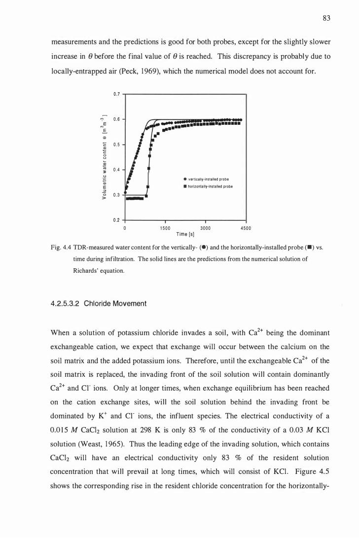
83
measurements and the predictions is good for both probes, except for the slightly slower
increase in () before the final value of () is reached. This discrepancy is probably due to
locally-entrapped air (Peck, 1969), which the numerical model does not account for.
0.7 -,-----------------,
-'? O.S E .... ........... • •••••• M oS ....
<t> .. C 0 .5 � c: 0 u CD ro 0 .4 � u "5 • vertically·lnstalled probe Q) E • horlzonta lly·lnslalled probe
.2 0 0 .3 >
0 .2 -t-----'T"""-----r------; o 1 500 3000 4500
Time [s]
Fig. 4.4 TDR-measured water content for the vertically- Ce) and the horizontally-installed probe C.) vs.
time during infiltration. The solid lines are the predictions from the numerical solution of
Richards' equation.
4.2.5.3.2 Chloride Movement
When a solution of potassium chloride invades a soil , with Ca2+ being the dominant
exchangeable cation, we expect that exchange will occur between the calcium on the
soil matrix and the added potassium ions. Therefore, until the exchangeable Ca2+ of the
soil matrix is replaced, the invading front of the soil solution will contain dominantly
Ca2+ and cr ions. Only at longer times, when exchange equilibrium has been reached
on the cation exchange sites, will the soil solution behind the invading front be
dominated by K+ and cr ions, the influent species. The electrical conductivity of a
0.0 1 5 M CaCh solution at 298 K is only 83 % of the conductivity of a 0.03 M KCI
solution (Weast, 1 965). Thus the leading edge of the invading solution, which contains
CaCh will have an electrical conductivity only 83 % of the resident solution
concentration that will prevail at long times, which will consist of KCl . Figure 4.5 shows the corresponding rise in the resident chloride concentration for the horizontally-
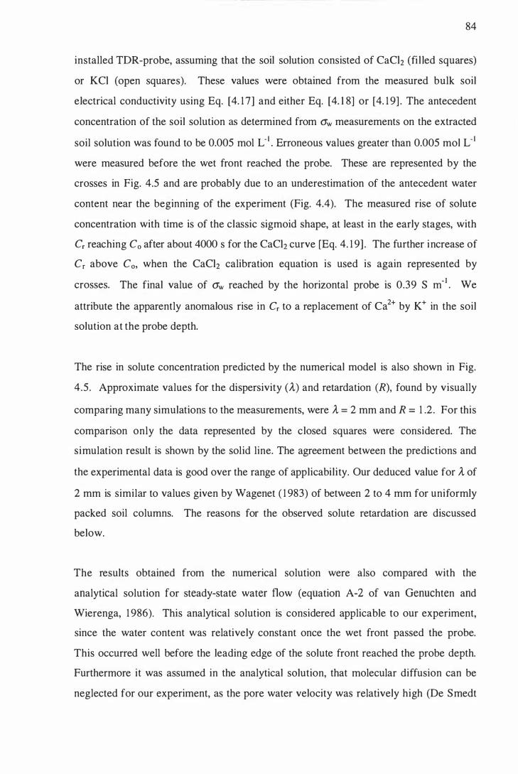
84
installed TDR-probe, assuming that the soil solution consisted of CaCh (fi l led squares)
or KCI (open squares). These values were obtained from the measured bulk soil
electrical conductivity using Eq. [4. 1 7] and either Eq. [4. 1 8] or [4. 1 9] . The antecedent
concentration of the soil solution as determined from (jw measurements on the extracted
soil solution was found to be 0.005 mol L-1 • Erroneous values greater than 0.005 mol L-1
were measured before the wet front reached the probe. These are represented by the
crosses in Fig. 4.5 and are probably due to an underestimation of the antecedent water
content near the beginning of the experiment (Fig. 4.4). The measured rise of solute
concentration with time is of the classic sigmoid shape, at least in the early stages, with
Cr reaching Co after about 4000 s for the CaCh curve [Eq. 4. 1 9] . The further increase of
Cr above Co, when the CaCh calibration equation is used is again represented by
crosses. The final value of (jw reached by the horizontal probe is 0.39 S m-I . We
attribute the apparently anomalous rise in Cr to a replacement of Ca2+ by K+ in the soil
solution at the probe depth.
The rise in solute concentration predicted by the numerical model is also shown in Fig.
4 .5 . Approximate values for the dispersivity (A) and retardation (R), found by visually
comparing many simulations to the measurements, were A = 2 mm and R = 1 .2 . For this
comparison only the data represented by the closed squares were considered. The
simulation result is shown by the solid line. The agreement between the predictions and
the experimental data is good over the range of applicability. Our deduced value for A of
2 mm is similar to values given by Wagenet ( 1 983) of between 2 to 4 mm for uniformly
packed soil columns. The reasons for the observed solute retardation are discussed
below.
The results obtained from the numerical solution were also compared with the
analytical solution for steady-state water flow (equation A-2 of van Genuchten and
Wierenga, 1 986). This analytical solution is considered applicable to our experiment,
since the water content was relatively constant once the wet front passed the probe.
This occurred well before the leading edge of the solute front reached the probe depth.
Furthermore it was assumed in the analytical solution, that molecular diffusion can be
neglected for our experiment, as the pore water velocity was relatively high (De Smedt

85
and Wierenga, 1 978). The analytical solution was fitted to the CaCh data using a least
square optimisation and is shown in Fig. 4.5 as the broken line. Values obtained for A and R were 2.3 mm and 1 . 1 5 respectively, and are comparable to those values used in
the numerical model. Hence we contend the numerical model is unlikely to be plagued
by any large errors due to numerical dispersion. We are thus confident that our
numerical model wil l work in the field, where transient water content effects may be
longer lasting.
0.035
� 0.030 C l' 0 '0 oS <.> 0.025 U> c
.S! � 0.020 c Q) 0 c 0 0 .0 1 5 0
"C Q) OJ + .S 0 .01 0 + + + +
u; + + + • Equallon [ 4 . I 8 ) 'P D Equation [4.19) ex: Cl 0.005 + + + + + + + shorl a n d long lerm I- dala
0.000 -t-----.-------r-----; o 1 500 3000 4500 Tim e [s]
Fig. 4.5 The resident concentration estimated from the TDR-measured bulk soil electrical conductivity
of the horizontally-installed probe during infiltration of KCl, using either Eq. [4. 1 8] (0) or
[4. 1 9] (.) . The fitted numerical solution of Eq. [4.4] is shown as the solid line and the
analytical solution as the broken line. Also shown are short and long term data (+), which were not used for the fitting.
The rise in electrical conductivity of the soil solution (jw) for the vertically-installed
TDR-probe is shown in Fig. 4.6. The gradual increase in (jw is due to the fact that the
TDR measures the average concentration over the entire 1 00 mm of the probe. Also
shown in Fig. 4.6 are the predictions from the numerical model, assuming the soil
solution contains either KCI (solid line) or CaCh (broken line), again using the values of
the transport parameters A and R that were obtained from the horizontal probe. The
predictions are based on the average concentration over the probe length, from which
the average electrical conductivity of the pore water was then obtained, using either Eq.

86
[4. 1 8] or [4. 1 9] , and assuming e to be constant. As might be expected, the measured
data first fol low the expected behaviour of CaCh (broken l ine), as the initial KCI soil
solution would be dominated by the exchanged CaCho However at later times the data
approach the sol id l ine for KCI, since at these longer times, more of the resident calcium
is likely to have been leached beyond the probe depth.
E � r! c: .g
.=! 0 '" .-0 '" Q) :; "0 �
.� <:; " "0 c: 0 0 n; 0 .'" <:; 2 w
0.5
0.4
0.3
0.2
0 . 1
0 .0 0
" , �
... ..----.-"'" - - - - - -.,� � - -
.. -.-,
/"
• vertlcally·lnstalled probe
1 500 3000 4500 T ime (5)
Fig. 4.6 The electrical conductivity of the soil solution calculated from the TDR-measured bulk soil
electrical conductivity of the vertically-installed probe (e) during infiltration of KCI. The
prediction from numerical solution of Eq. [4.4], assuming the soil solution to contain either
CaCh broken line) or KCl (solid line).
The reason for a retardation value R of 1 .2, which implies a Kd of 0. 1 43 L kg- I , warrants
further discussion. The Ramiha silt loam contains some allophanic material, and is
therefore likely to have some positively-charged sites at the existing soil pH of 5 .5 .
Therefore we would expect some chloride to be adsorbed onto anion exchange sites.
Indeed, our measurements of chloride concentration in the soil solution extracted from
soil samples taken at the end of the experiment indicated that some chloride had in fact
been adsorbed. On average 1 3 % more chloride was present than would be expected if
Co was the concentration in the soil solution. However if another anion (e.g. nitrate or
sulphate) were exchanged for the adsorbed chloride, there would be l ittle effect on the
electrical conductivity of the soil solution. This is because these anions have similar
equivalent electrical conductivities (Weast, 1 965). In contrast to miscible displacement
studies where the actual chloride concentration is measured, the TDR technique would

87
not be able to detect the chloride adsorption and retardation. Only if the invading
solution caused a change in the anion adsorption capacity (ABC) would the TDR
electrical conductivity measurements detect any solute retardation. Thus independent
measurements were made of the effect of the external solution concentration on the
ABC of the Rarniha soil . The results are shown in Fig. 4.7.
0 .9 0 .8 •
C> .><: '0 0.7 E � 0.6 .� u '" a. 0.5 '" u Q) 0.4 C> c '" 0.3 .<:: u x Q) 0.2 c .2 c « 0 . 1
0 .0 0 .00 0 .0 1 0.02 0.03 0.04 0.05 0 .06
C oncentration [m o l L '1 J
Fig. 4.7. The anion exchange capacity (e) measured for various concentrations of KCI in the soil
solution. The solid line is the relationship between the anion exchange capacity and the
external solute concentration with a slope of 0. 14 L kg'l .
Here it can be seen that the ABC is strongly dependent on soil solution concentration
over the range of interest, namely 0.005 to 0.032 mol L' I . Further the relationship,
shown as the solid l ine in Fig. 4.7, is approximately linear, with a slope of 0. 1 4 L kg- I .
Note that this is almost identical to the Kd value appropriate for an R value of 1 .2.
4.2.6 Conclusions
The study has demonstrated that combining TDR and disc permeametry provides a
useful tool for characterising water flow and chemical transport. The use of both
vertically- and horizontally-installed TDR-probes can provide values for transport
parameters as well as independent verification of these values. The importance of
accurate measurement of e is stressed, as this can have a large influence on the

--- ------------------------
88
calculation of the resident solute concentration. The dispersivity (A) and the retardation
(R) at the imposed pressure head of -50 mm were deduced to be 2.3 mm and 1 .2,
respectively.
In previous studies using TDR to measure solute movement in soi l , it has been assumed
that solute concentration is proportional to electrical conductivity. Any effects of cation
or anion exchange on the TDR measurement of the soil electrical conductivity have
been ignored. We have shown here how important these effects can be. When KCI was
appl ied, even when enough solution had been added to the soil to make the chloride
concentration in the soil solution similar to that in the appl ied solution, exchange of K+
with Ca2+ was the apparent cause of the electrical conductivity of the soil solution being
quite different to that of the applied solution.
This finding has a number of implications. One is that it is important that actual soil
solution extracts be used when the TDR technique is being calibrated for soil solution
electrical conductivity measurements. Another implication is that when the TDR is
being used to measure solute movement in soil , cation (and sometimes anion) exchange
needs to be taken into account. Preleaching with a calcium salt solution may therefore
sometimes be appropriate. Alternatively, if the cation exchange sites are already
calcium dominated, a calcium salt should be used as the tracer when solute movement
parameters are being measured.
The method need not be restricted to laboratory studies as we have applied here. It should be possible to determine in situ not only the hydraulic properties that control
infi ltration, but also the chemical transport characteristics that determine the distribution
of the associated solutes. We plan to carry out further investigations in the field using
free-standing undisturbed pedestals that have been specially excavated to accept a disk
permeameter on top. Here water and solute movement can be simply described one
dimensionally. Vertically- and horizontally-placed TDR-probes will again be used.
Since water movement from the disk, will be transient, the numerical model will again
be needed for the inverse simulation of the chemical transport properties.

89
Acknowledgments The authors gratefully acknowledge the help provided by Dr.G.N. Magesan of Manaaki
Whenua Landcare Research, Hamilton, and Nobiru Kozai, Kumamoto Prefectural
Research Station, Japan. This research was funded by FRST contract C09227.
4.3 TDR and Undisturbed Soil Columns of Manawatu Fine Sandy Loam
As a next step the use of TDR in combination with disk permeametry was assessed
using undisturbed soil columns of Manawatu fine sandy loam. The experimental setup
was the same as described in Section 5.2, except that one of the TDR probes was
installed vertically through the disk permeameter as described in Section 4.2. Highly
preferential flow of the appl ied chloride solution was observed in the effluent, as well as
by TDR. Although the TDR probes were inserted into predril led holes, vertical cracks
might have developed during their insertion. Significant preferential flow is expected
only in continuous vertical channels, which are at least 0.2 mm in diameter, or cracks of
least 0. 1 mm width and at pressure potentials above - 1 50 mm (Scotter, 1 978). As the
solution was applied via a disk permeameter set to a pressure potential of -50 mm,
cracks might be the reason for the observed preferential flow. Another possibility is
preferential flow along the vertical probe (Zeglin et al., 1 992) .
These results show that care must be taken when using vertically installed TDR probes
in undisturbed soil columns. Often, insertion without significant side-effects may be
difficult.

90
4.4 TDR Estimation of the Resident Concentration of Electrolyte in the
Soil Solution
4.4.1 Abstract
by Iris Vogeler , Brent E. Clothier , and Steven R. Green
From Australian Journal of Soil Research, 1 997, 35, xx.
In order to examine whether the electrolyte concentration in the soil solution can be
estimated by TDR-measured bulk soil electrical conductivity, column leaching
experiments were performed using undisturbed soil columns during unsaturated steady
state water flow. The leaching experiments were carried out on two soi ls with
contrasting pedological structure. One was the strongly structured Rarniha silt loam,
and the other the weakly structured Manawatu fine sandy loam. Transport parameters
obtained from the effluent data were used to predict the transient pattern in the resident
electrolyte concentration measured by TDR. The electrolyte concentration was inferred
from the TDR-measured bulk soil electrical conductivity using two different calibration
approaches; that resulting from continuous solute application, and the other by direct
calibration. Prior to these, calibration on repacked soil columns related TDR
measurements to both the volumetric water content, and the electrolyte concentration
that is resident in the soil solution. The former calibration technique could be used
successfully to describe solute transport in both soils , but without predicting the
absolute levels of solute. The direct calibration method only provided good estimates of
the resident concentration, or electrolyte concentration, in the strongly structured top
layer of the Rarniha soil . This soil possessed no immobile water. For the less
structured layer of the Rarniha, and the weakly structured Manawatu soi l , only crude
approximations of the solute concentration in the soil were found, with measurement
errors of up to 50%. The small-scale pattern of electrolyte movement of these weakly
structured soils appears quite complex.
Keywords: TDR calibration, solute transport, resident concentration, soil water content,
soil structure.

9 1
4.4.2 Introduction
Time Domain Reflectometry (TDR) is a relatively new technique that possesses
potential for studying solute transport through the soil (Kachanoski et al. , 1 992; Wraith
et ai., 1 993 ; Vanc100ster et ai. , 1 993, 1 995) . This technique relies on the measurement
of the impedance (ZL), or bulk soil electrical conductivity (cr), which can be related by
cal ibration to the solute resident concentration (Cr). TDR calibration has been the prime
topic of many studies, and it is already well known that the volumetric water content (9),
the electrical conductivity of the soil solution (aw), the surface conductance (as), as well
as the bulk density, and the soil temperature affect the TDR-measured bulk soil
electrical conductivity. However, the overall effect of these various factors on (J, as
measured by resistivity techniques, is not yet fully understood. Various approaches have
been adopted to relate a and Cr. These have been discussed in detail by Mallants et ai.
( 1 994; 1 996), and Ward et ai. ( 1 994). Here only the direct calibration, using both
repacked and undisturbed soil columns, and the continuous solute application approach
are described. Both have potential to measure solute transport through undisturbed soil
columns in the laboratory, and also directly in the field.
In the direct calibration approach, the TDR-measured impedance (Zd - or bulk soil
electrical conductivity (a) - is related to the concentration of the soil solution (aw) and
the water content (8). The calibration is generally performed on homogeneously
repacked soil columns, in which both the soil structure and pore size distribution are
disturbed. This change in structure and pore tortuosity is likely to affect the calibration
function (Rhoades et ai. , 1 976; Nadler, 1 98 1 ) . Nadler ( 1 99 1 ), however, found the effect
of structural disturbance on (J-(Jw relations to be smal l . Briefly, soil samples are
equilibrated to various water contents using different solution concentrations. Once a
relation between a, aw, and 8 has been found, it should in theory be possible to study
solute transport in situ under transient conditions. The first such direct calibration was
presented by Rhoades et al. ( 1 976). They used a four-electrode resistance technique.
The calibration approach was based on a constant surface conductivity, a l inear
relationship between a and aw, plus a tortuosity factor. However several investigators
have found a dependency of the surface conductance on salt concentration and water

92
content (Cremers et aI. , 1 966; Nadler, 1 98 1 ; Ward et al., 1 994). The latter was
incorporated in our previous calibration (Section 4.2), and has also been discussed by
Mallants et ai. ( 1 996).
Another approach involves a continuous solute application, by which solute is appl ied
until a constant (j is reached. This asymptote is, in the absence of other information,
then simply equated to the input concentration Co. Thus it is assumed that the solute has
spread uniformly throughout the soi l . But in soi ls with immobile water, the
equilibration time between the two water domains might be long, so that application of
this method would require a long solute appl ication time (Mall ants et ai. , 1 996).
However several experimental studies have used this continuous solute appl ication
method with TDR to obtain solute transport parameters from leaching experiments
(Mall ants et al., 1 994; Section 5 .2) . The approach is however restricted to steady-state
conditions. In the field, water and solute transport are often transient in nature. This
then makes the direct calibration method more suited for studying solute transport at the
field scale, despite its attendant problems.
The purpose of this study was to determine if the electrolyte concentration in the soil
solution could be estimated from the (j measured by TDR, as based on the direct
cal ibration approach. Furthermore we compared various calibration approaches to
monitor by TDR solute transport through undisturbed soil columns under unsaturated
steady-state water flow. Two structurally different soils were studied: the Manawatu
fine sandy loam, a soil classed by pedologists as being weakly structured, and the
Ramiha silt loam, a soil classed as being strongly aggregated (Cowie, 1 978; Pollok,
1 975).
4.4.3 Theory
The theory for monitoring solute transport by Time Domain Reflectometry has already
been reviewed in detail in Section 4.2, amongst others, so only salient features are
repeated here. Briefly, the estimation of the solute resident concentration by TDR is
based on the measurement of the dielectric constant (EO) and the impedance (Zd of the

93
soil . The dielectric constant can be used to calculate the volumetric water content (8),
using either the so-called "universal" relationship found by Topp et al. ( 1 980), or by
specific calibration. The impedance can be related to the bulk soil electrical
conductivity by (Nadler et al., 1 99 1 )
[4.20]
Here KG is a geometric probe constant which has been previously determined (Section
4.2), and Ie is a temperature-correction coefficient (see Table 1 5 , U.S. Salinity
Laboratory Staff, 1 954).
4.4.4 Materials and Methods
The TDR used for the experiments was a 1 502 C Tektronix cable tester (Tektronix,
Beaverton, OR). Three-rod probes of length of 100 mm, diameters of 2 mm, and
spacing between the center and outer rods of 1 2.5 mm, were used for all measurements.
The probes were connected, via a 50 n coaxial cable and a multiplexer, to the cable
tester. The cable tester was controlled by a laptop computer which automatically
analysed for water content and bulk soil electrical conductivity.
Two soils with contrasting pedological structure were studied. One was the alluvial
Manawatu fine sandy loam (a Dystric Fluventic Eutrochrept), a weakly structured soil.
The other was the aeolian Ramiha silt loam (an Andie Dystroehrept), a strongly
aggregated soil with variable charge due to volcanic ash addition. Description of both
soils are given in Clothier et al. ( 1 996) . The Manawatu soil was taken from the
herbicide strip in the Massey University Orchard. The Ramiha soil was taken under
pasture. For each soil , two free-standing soil columns were carved from the soil profiles
after removing the top 20 mm. These will be referred to as column A and B for the
Manawatu soil, and column C and D for the Rarniha soi l . Additional soil samples were
taken for the cal ibration measurements.
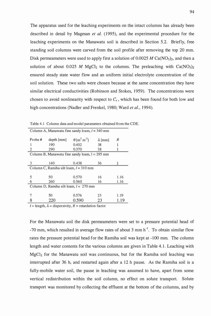
94
The apparatus used for the leaching experiments on the intact columns has already been
described in detail by Magesan et al. ( 1 995), and the experimental procedure for the
leaching experiments on the Manawatu soil is described in Section 5.2. Briefly, free
standing soil columns were carved from the soil profile after removing the top 20 mm.
Disk permeameters were used to apply first a solution of 0.0025 M Ca(N03h. and then a
solution of about 0.025 M MgCh to the columns. The preleaching with Ca(N03h
ensured steady state water flow and an uniform initial electrolyte concentration of the
soil solution. These two salts were chosen because at the same concentration they have
similar electrical conductivities (Robinson and Stokes, 1 959). The concentrations were
chosen to avoid nonlinearity with respect to Cr , which has been found for both low and
high concentrations (Nadler and Frenkel, 1 980; Ward et al. , 1 994).
Table 4 . 1 Column data and model parameters obtained from the CDE.
Column A, Manawatu fine sandy loam, 1 = 340 mm
Probe # depth [mm] (J [m3 m'3] A [mm] R
1 1 90 0.402 38 2 290 0.370 38 Column B , Manawatu fine sandy loam, 1 = 295 mm
3 140 0.438 36 Column C, Ramiha silt loam, 1 = 3 1 0 mm
5 50 0.570 1 6 1 . 1 6 6 260 0.560 16 1 . 1 6 Column D, Ramiha silt loam, 1 = 270 mm
7 50 0.576 23 1 . 19 8 220 0.590 23 1 . 1 9 I = length, ..:t = dispersivity, R = retardation factor
For the Manawatu soil the disk permeameters were set to a pressure potential head of
-70 mm, which resulted in average flow rates of about 3 mm h' l . To obtain similar flow
rates the pressure potential head for the Ramiha soil was kept at - 1 00 mm. The column
length and water contents for the various columns are given in Table 4. 1 . Leaching with
MgCh for the Manawatu soi l was continuous, but for the Ramiha soil leaching was
interrupted after 36 h, and restarted again after a 1 2 h pause. As the Ramiha soil is a
ful ly-mobile water soil , the pause in leaching was assumed to have, apart from some
vertical redistribution within the soil column, no effect on solute transport. Solute
transport was monitored by collecting the effluent at the bottom of the columns, and by

95
TDR probes inserted horizontally into the soi l columns. Two probes were inserted into
each column, the depths and probe numbers are given in Table 4. 1 .
Solute transport was modelled using the convection dispersion equation (CDE), and the
solutions given by van Genuchten and Wierenga ( 1 986) for flux concentrations (their
A I ), for the effluent, and resident concentrations (their A2) for the TDR data.
4.4.4.1 TDR Calibration
The calibration procedure for the Ramiha silt loam calibration has already been
described in Section 4.2. Air dried, sieved soil « 2 mm) was stepwise brought to water
contents ranging from 0.3 to 0.6 using KCI solutions of 0.0 1 , 0.03, and 0.05 M. At each
water content the soil was packed, at a bulk density of 0.84 Mg m-3, into acrylic columns
with a height of 250 mm and a diameter of 1 20 mm. The dielectric constant and the
electrical impedance of the soil was measured by three-rod TDR probes inserted
horizontally into these soil columns. After measurement, the water content was
determined gravimetrically, as wel l as the electrical conductivity of the pore water by
high speed centrifuging, and measurement of the electrical conductivity of the
supernatant using a conductivity meter. The same procedure was now used for the
calibration of the Manawatu fine sandy loam, but the soil was packed to a bulk density
of 1 .35 Mg m-3, and only two concentrations, 0.005 and 0.025 M MgCh and two water
contents of 0.35 and 0.45 were used. The leaching experiments were performed in the
same concentration range as the calibrations.
Additionally, calibration measurements for the Manawatu soil were carried out on
undisturbed soil columns. Steel cylinders, 1 1 0 mm high and 1 00 mm in diameter, were
used to enclose undisturbed pedestals of soil from adjacent to where the soil columns
were taken for the leaching experiment. The metal of the cylinders did not have an
effect on the TDR readings. The undisturbed soil cores were taken into the laboratory
and wetted by capillary rise using again the two solutions of 0.005 and 0.025 M MgCh.
After wetting, the samples were left to equilibrate in a pressure apparatus using two
different pressures of 30 mbar and 2 bar. For each combination of concentration-

96
pressure, 4 replicate columns were used. For measuring £ and cr the TDR probes were
installed vertically from the top. For each combination, duplicate measurements were
made, giving 32 measurements in total . Again the gravimetric water content and the
electrical conductivity of the pore water were determined, but only a single cylindrical
soil sample around the probes was used.
4.4.5 Results
4.4.5.1 Water Content Calibration
The calibration curve for the £-() relationship for the Rarniha silt loam has already been
given in section 4.2. Due to the high organic matter content and the low bulk density of
0.84 Mglm3 for this soi l , a deviation of about + 0. 1 m3 m-3 was found between the
relationship found and the curve suggested by Topp et al. ( 1 980). For the Manawatu
fine sandy loam, with a bulk density of 1 .35 Mg m-3, the relationship of Topp et al.
( 1 980) was found to be adequate for the range 0.05 � () � 0.46 m3 m-3. The maximum
deviation was just 0.024 m3 m-3.
4.4.5.2 Solute Concentration Calibration
The relationship between the bulk soil electrical conductivity, the water content, and the
electrical conductivity of the soil solution of repacked Rarniha soil was in Section 4.2 to
be capable of description by,
cr - (a () - b) cr = -,----:--
W (c () - d) [4.2 1 ]
where a, b, c, and d are constants.
The results, using the same approach for the Manawatu soil are shown in Fig. 4.8. Both
the measurements obtained from the disturbed soil column (squares), and the
undisturbed columns (circles) are given. Also shown are the standard deviations

97
(vertical bars) from the measurements on the disturbed soil columns. The water content
in the undisturbed soil columns ranged from about 0.4 1 to 0.47 m3 m-3, but only those
samples of either 0.42 or 0.44 m3 m-3 ( ± 0.007) were used for the solute calibration.
This resulted in 10 and 6 measurements for the two water contents. Linear relationships
between a and aw were found for the disturbed soil , and were assumed for the
undisturbed soil columns at each water content. These relationships are shown on
Fig.4.8. Using the same approach as described in Section 4.2 a relationship of the form
of Eq. [4.2 1 ] was found between a, aw, and () for both the disturbed soil columns, and
the undisturbed soil columns. As the values of a, b, c, and d in Eq. [4.2 1 ] are unique to
each soil they are not explicitly given here.
_ 0 . 1 6 +------------'------r E ,� � b � 0 . 1 2 > � U ::l
'0 c:: g 0 .08 ell u ''::: c:; <1> <1> 0.04
9 = 0.45 '
9 = 0.44
, 9 = 0.42 , ' 9 = 0.35 ,
0.00 +-----.--------r----+ 0.0 0.2 0.4 0.6
E lectrical conductivity of the soi l so lu ti on OW [ S m ·l )
Fig. 4.8 TDR-measured bulk soil electrical conductivity vs. electrical conductivity o f the soil solution
measured with a conductivity meter for different water contents for Manawatu fine sandy loam
using disturbed (D) and undisturbed (0,.) soil columns. Also shown is the standard deviation
(vertical bars) and fitted relationship (solid and broken lines).
The solute concentration, C, [mol r1 ] for MgCh solution at concentrations ranging from
0.005 to 0.025 M can then be calculated from aw [S m:l ] using data from Weast ( 1 965)
as
[4.22]

98
4.4.5.3 Leaching Experiments
Manawatu: The results of the leaching experiments on Manawatu fine sandy loam are
described in Section 5 .2 . The effluent data were used to obtain parameters for the
convection-dispersion equation of solute transport. The values for the dispersivity were
36 and 38 mm for Column A and Column B. These were then used to predict the
resident concentrations of chloride (Cr) that should be measured using the continuous
solute application method. Only one of the probes in Column B could be used as, for
unknown reasons, the other gave unrealistically high measurements of the impedance.
The results from the other probes are shown in Fig. 4.9. The agreement between the
simulation and the TDR-inferred solute concentration, using the continuous solute
application method, is good except for probe 2. Considering that the TDR measures
only a small volume around the probe, whereas the effluent averages the concentration
over the total area studied, this agreement is nonetheless heartening. Any variations in
water content or salt concentration in the cross section can have an effect on TDR
measured cr. However considerable replications would overcome this problem.
Also shown in Fig. 4.9 are the TDR-estimated relative concentrations of chloride using
equation [4.2 1 ] and [4.22] , with the constants found either from the calibration on
repacked or undisturbed media. For column A, the Cr estimated from the calibration on
disturbed soil (open squares) are higher than the input concentration, by up to about
50% for probe 3. These deviations could be due to a different soil structure or pore size
distribution from that in the disturbed soil columns used for calibration, or perhaps due
to small variations in probe soil contact. Furthermore, the Cr calculated from the
relation for the undisturbed soil columns (open circles), are even higher. This could be
due to the lower water content in this column compared to that used for the calibration
(Table 4. 1 ) . Extrapolating the linear relationship found at e of 0.42 and 0.44 m3 m-3
might not have been appropriate. The overestimation of CTw might hence be due to the
assumption of linearity outside the calibration range. Yet for the probe in column B , the
agreement between the prediction from the effluent and the TDR-estimated
concentration is reasonable, whether using calibration on undisturbed or repacked
media. We note that this soil column had a water content of 0.438, which is within the

99
range used in the calibration with undisturbed soil columns. Although the good
agreement between TDR-estimated Cr and the prediction in column B might only be
fortuitous, it seems that TDR can be used to measure solute resident concentrations,
provided that calibrations have been carried out on undisturbed soil samples, and were
within the water content and aw range.
2 .0
1 .5
o U U � 1 .0 0-t>
0.5
0.0
0
1 .0
0.8 0
u u 0.6 � � 0.4
t> 0.2
0.0
0
(a)
00
r9 o cP o Dl 0 0
gjl ••
Q] •
20 40 60 T i m e [hI
20 40 60 Tim e [h )
0 0 0 0
-...lI...--.
80 1 00
0 •
80 1 00
0
(b)
o
o o
o 0
o 0 o
0 0
0 0
0 0
o 0 rSXP
o
20 40 60 Tim e [hI
o
o
o 0
o 0
80 1 00
Fig. 4.9 Normalised bulk soil electrical conductivity as measured by TDR (e) and simulated curves (solid
lines) for column A: (a) probe 1 , (b) probe 2, and column B: (c) probe 3. Also shown are the
normalised resident concentrations calculated from TDR measurements, and using Eq. [4.2 1 ] with
values obtained from measurements on disturbed (D) or undisturbed columns (0), and Eq. [4.22].

1 00
Ramiha: The normalised effluent concentrations of chloride from the Ramiha soil in
columns C and D, are shown in Fig. 4. 1 0, together with the fits to the CDE.
Dispersivities of 1 6 and 23 mm and were found for the two columns. Furthermore, a
l inearised retardation for the chloride of about 1 .2 was obtained. This reaction is
consistent with the value given in section 4.2, and is due to positively charged exchange
sites at a pH of 5 .5 . The anion exchange capacity increases with a rise in the electrolyte
concentration of the soil solution, such that the TDR should also detect this retardation.
1 .0
O .B
0.6 c
l:2 (.) 0 .4
0 .2
0.0 0 1 00 200 300 400
Q [m m )
Fig. 4. 10 Normalised anion breakthrough data and fitted curves using the CDE for column C (e and solid
line) and column D (. and broken line).
The dispersivities and the retardation factor so found, were now used to predict the
resident concentration, again using the CDE, as should be measured by the TDR probes.
The results are shown in Fig. 4. 1 1 . The somewhat minor variation in (j measured by
probe 5 and 7 could be due to the decrease in water content of 0.028 and 0.0 1 7 m3 m-3
close to the soil surface after interruption of leaching. For the lower probes the water
content remained constant. Using the continuous solute application method, the
agreement between the prediction and the measurements is again good for all 4 probes.
The water content calculated from the TDR calibration on repacked columns (eq. [4. 1 6])
were consistently 0.05 m3 m-3 higher than the gravimetrically determined ones (Table
4. 1 ) . This could simply be due to a slightly higher mean bulk density (Ph) of 0.89 Mg
m-3 found for the columns, compared to the calibration which was performed at a Ph of

1 0 1
0.84 M g m-3 . This shows that the calibration curve is highly sensitive to Pb, and again
stresses the need for care when using TDR calibration procedures. Consequently to
calculate the normalised solute resident concentrations (Cr) the gravimetrically
determined e were used with Eq [4.2 1 ] and [4.22]. These are shown in Fig. 4. 1 1 as the
open squares.
1 .0
o () () o 0.5 b----b
0.0
1 .0 0 () -() �
0.5 \:)----\:)
0 50 1 00 1 50 200 0 T ime [h]
°I§PQjJ CIJ
(c)
0.0 ...---,-----,---r----, 50 1 00 1 50 200 0
Tim e [h]
��rrDrn I . ......--0 , · 0 .. E1. (b)
50 1 00 1 50 200 T ime [h]
F iDPoCfJ cP
o/� . '" °IJ (d)
50 1 00 1 50 200 Tim e [h]
Fig. 4. 1 1 Normalised bulk soil electrical conductivity as measured by TDR (e) and simulated curves
(solid lines) for column C: (a) probe 5, (b) probe 6, and column D: (c) probe 7, and (d) probe 8.
Also shown are the normalised resident concentrations calculated from TDR measurements, and
using [4.2 1 ] and [4.22] (0).
The agreement between the prediction is good just for the two probes installed at 50 mm
(probes 5 and 7), considering that e changes due to interruption of leaching were
ignored. For the two other probes installed at 260 and 220 mm, the calculated Cr is
again far too high. This is again likely to be due to the local sensitivity of the TDR-

1 02
measured impedance or bulk soil electrical conductivity to soil structure, and perhaps
bulk density immediately adjacent to the probe-rods. Both increase with depth. The
structure of the Ramiha silt loam changes at a depth of 80 mm. The soi l changes from
strongly to medium developed aggregates, and the organic matter content decreases
(Pollok, 1 975). These changes in the soil profile are considered to explain the good
agreement found for the upper probes, and the discrepancies found for the lower probes.
The strongly developed structure in the top 80 mm appears to behave, in a electrolytic
sense, similarly to a repacked soil . However the weaker pedological structure of the
deeper profile apparently has quite an effect on the TDR-measured a.
4.4.6 Conclusions
The TDR has been shown to be useful in estimating solute transport parameters, but
only when the relative bulk soil electrical conductivity was used in the continuous solute
application approach.
For two soils with contrasting pedological structure, the continuous solute application
method performed well . However a drawback of this method is the need to ensure a
constant water content and steady state flow. In the field however the water content is
generally variable both in time and space. A further drawback is that this method does
not provide an independent measure of the final resident concentration. Hence it is not
possible to use the asymptotic values of Cr to infer anything about the degree of mobility
of soil water. The success with the continuous solute application method, indicates that
in some practical applications such a crude estimation might be sufficient. But for
accurate predictions of resident concentrations, and solute transport under transient
water flow further studies are needed on the various and local heterogeneities on TDR
measured a and a-aw-8 relationships. Separate calibrations for each layer might well
always be necessary.
Caution has to be exercised when estimating electrolyte levels in the soil solution from
TDR-measured a using a-aw-8 relationships obtained from disturbed soil columns.
1 03
Whereas this direct-calibration approach was found appropriate for the strongly
aggregated layer of the surface Ramiha silt loam, it overestimated the resident
concentrations in the less structured lower profile of the Ramiha soi l . Also it failed to
perform in the weakly structured Manawatu fine sandy loam. In a study on undisturbed
saturated soil columns MaIl ants et ai. ( 1 996) also found that the reference impedance
was underpredicted by 50% when using the direct calibration approach, based on
independent calibration measurements in repacked soil columns.
Our results suggest a high sensitivity of the TDR-measured bulk soil electrical
conductivity to the local soil structure, texture, and perhaps bulk density immediately
surrounding the probes, and to the probe-soil contact. S imilar findings were made by
Vanclooster et al. ( 1 995). In their study of solute transport through 1 m long monoliths
they had to calibrate each probe separately. This was, in their case, attributed to changes
in soil chemical properties within the soil profile.
It is interesting to note again that soils of weak pedological structure, e.g. the Manawatu,
display quite complex hydraulic functioning (Clothier et ai., 1 995). In contrast, soils of
strongly developed structure, e.g. the Ramiha, can exhibit quite simple hydraulic
functioning that is amenable to straight forward analysis (Clothier et ai. , 1 996) . The
TDR procedures used here reinforce the contrast between pedological structure and
hydraulic functioning.
Acknowledgments We thank Dave Scotter (Massey University, Palmerston North) for assisting with the
experiments, and Arie Nadler (The Volcani Center, Institute of Soil and Water, Bet
Dagan 50250, Israel) for helpful comments. This research was supported by the NSOF
96- 1 70 "Partitioning of rootzone chemical into either uptake or despatch".

1 04
4.5 Overall Conclusions
The TDR method has been shown useful for monitoring solute transport through
a repacked soil column under transient water flow (Section 4.2) . Direct calibration was
used, which related the TDR-measured impedance at various water contents to the pore
water electrical conductivity in undisturbed soil columns . TDR probes installed both
horizontally-and vertically installed TDR-prgbes were used successful. Furthermore the
experiment demonstrated the effect of cation exchange reactions on the TDR-measured
bulk soil electrical conductivity. This is important when the infiltrating solution is
composed of cations different to those dominanting the exchange sites . In this case
exchange reactions altered the electrical conductivity of the soil solution, which had a
large effect on the TDR inferred solute transport parameters. The behaviour of chloride
was simulated by coupling the water flow equation with the convection-dispersion
equation. However the simulations were only reasonable when appropriate assumptions
concerning the accompanying cation were made.
When TDR probes were installed vertically into undisturbed soil columns, highly
preferential flow was observed. This probably resulted from cracks, which developed
during their insertion. This demonstrates that, in some situations using vertically
installed TDR probes in the field to monitor solute transport can lead to erroneous
results.
In undisturbed soil columns of two contrasting soils, TDR only proved useful for
monitoring solute transport if the continuous solute appl ication approach was used
(Section 4.4). However, this approach is limited to steady-state water flow, and
problems arise in soils with mobilelimmobile water fractions. Solute concentrations
inferred from the TDR measured bulk soil electrical conductivity, and using the direct
calibration approach, overestimated the resident concentrations in most cases. This was
probably due to the high sensitivity of TDR measurements to soil structure, and bulk
density immediately adjacent to the probe wires.

1 05
In conclusion, the TDR technique for monitoring solute transport in undisturbed soils
has several problems associated with it. These include the effect of the soil structure,
bulk density and the composition of the soil solution on TDR measured dielectric
constant and impedance. Furthermore TDR measures only the total ionic concentration
of the soil solution, not that of the individual ions. The technique seems therefore
unsuitable for studying transport and exchange of reactive solutes.
Under steady-state water flow, the TDR-technique seems to be a valuable tool for
determining solute transport parameters in undisturbed soil columns, as well as in the
field. The use of TDR to monitor solute movement under transient water flow is
hampered by a good understanding on how the TDR-measured impedance is influenced
by soil structure and bulk density. But the continuous application method could
overcome this, if some independent measure were made of the final concentration.

1 06
Chapter 5
5. Anion Movement Through Unsaturated Soil
5. 1 Introduction
In Chapter 2 various approaches to characterise solute transport have been described and
compared. It was concluded that the convection dispersion equation (CDE) seems a
promising model to describe solute transport during unsaturated flow, but it still needs
further testing. Apart from being relatively simple, transient water flow, as well as ion
adsorption and exchange can be easily incorporated into the CDE. The leaching
experiments described in this chapter were performed to test the ability of the CDE to
describe anion movement under various water flow regimes. Also considered is the
mobile/immobile water approach. Furthermore, the effect of the initial soil water and
the vegetation on solute transport was studied.
In the prevIous Chapter, the TDR technique for studying solute transport through
repacked and undisturbed soil columns was described. It was concluded that
considerable replication of TDR instrumentation is needed to accurately describe solute
transport, and there were certain problems with calibration. In this Chapter the more
conventional method of using outflow breakthrough curves (BTC) to monitor solute
movement is described for the same undisturbed soil columns. By using the BTC,
average solute transport parameters over the entire soil column are obtained. These
would be more spatially representative for solute transport compared to local
measurements obtained by TDR probes. Furthermore, by collecting and analysing soil
solution samples, solute exchange reactions between the soil solution and the soil matrix
can be studied. These cannot be detected by TDR. The use of suction cups to study
solute transport is also assessed.
The first paper describes leaching experiments on undisturbed soil columns of
Manawatu fine sandy loam under a bare soil surface. These experiments were carried
out to examine the effect of the water flow velocity on solute dispersion, and to test the
validity of assuming a velocity invariant dispersivity. The second paper describes

107
leaching experiments performed on the same soi l , but now under pasture. The effect of
a short pasture, as wel l as that of the initial water content on solute transport is
investigated. For these experiments a rainfal l simulator was bui lt. A picture of the
experimental setup for the experiments described in Section 5.3 is shown in Fig. 5 . 1 .
Final ly the approach of Bolt ( 1 982) for describing dispersion, discussed in Section 2.5.3 ,
is tested using the model parameters of the CDE and the MIM obtained from the various
experiments.
The computer programs used in Section 5.2 were written in QuickBASIC, and are
described in Appendix A. Examples of the various programs used in the fol lowing
experiments are given in Appendix B, Programs 1 -3 . The computer program used in
Section 5 .3 was written in FORTRAN, and the solution was based on the Crank
Nicholson finited-difference scheme, which is described in detai l in the 'WAVE' model
by Vanclooster et al. ( 1 994).
Fig. 5 . 1 Experimental setup for the experiments described in Section 5 .3 .

1 08
5.2 Anion Transport Through Intact Soil Columns During Intermittent Unsaturated Flow
by Iris Vogeler, David R. Scotter, Brent E. Clothier, and Russel W. Tillman
From Soil Technology, in press
5.2.1 Abstract
To assess the effect of varying water flow velocities on solute transport, leaching
experiments were conducted on undisturbed soil columns of Manawatu fine sandy loam.
A leaching apparatus, applying pressure heads of -80 mrn or -3 mrn to both ends of the
columns, was used to infiltrate solutions of either MgCh, or Ca(N03)2, at water flow rates
of either 3 or 1 3 mrn h- I . Intermittent rainfall events were simulated by performing 3
consecutive unsaturated leaching events with no-flow periods interspersed. Solute
transport was monitored by collecting effluent, and using suction cups and Time Domain
Reflectometry. The convection-dispersion equation was found to simulate the anion
breakthrough-curves well except for the short term concentration discontinuities
observed when flow resumed after an interruption. Dispersivities obtained with the
different measurement techniques and the two contrasting flow rates were similar, with
values between 25 and 59 mm. A 1 0% difference between the flux and final resident
concentrations was found, even after 1000 mrn of infi ltration over 1 3 days, attributable to
anion exclusion from the double layer water of about 0.04 m3 m-3. The discontinuity after
flow interruption could be simulated reasonably well using the mobilelimrnobile model
with three different soil water domains assumed: "mobile", "immobile", and
"exclusion".
5.2.2 Introduction
Practical relevance, combined with an unease concerning our present understanding,
motivates research on solute movement through structured soil. At a microscopic level we
know how convection and molecular diffusion can move water-borne solutes through soil .
We know that the local interaction between these two processes produces what we call

1 09
hydrodynamic dispersion. But these microscopic insights are of limited value when we
ask how a certain Darcy flux density of water might move a certain solute through a given
soi l .
Traditionally measurement of solute flow has involved either soil sampling, or the use of
suction cups. Soil sampling is tedious and destructive. With suction cups one is not sure
what mix of flux and resident concentration is being measured. The more recent advent of
time domain reflectometry (TDR) avoids these two problems, but has other limitations
associated with it, e.g. the small sampling volume, and the restriction to steady-state water
flow. Here we describe unsaturated experiments on intact soil columns in which we
real ise measurement of anion and cation transport by TDR and suction cups, and by
sampling effluent at the end of the column. These experiments allowed the assessment of
suction cups and TDR as techniques for characterising solute flow in intact soil at realistic
flow rates.
Most theoretical descriptions of solute flow involve the convection-dispersion equation
(CDE), although other models, such as the stochastic-convective model of Jury ( 1982)
have been used successfully to describe solute transport at the field scale. The CDE has
often been found inadequate in structured soils under saturated flow conditions. In the
field, however, such flow conditions are rare, especially in the more permeable macropore
hidden soils that are used for agriculture and water disposal . More cornmon is unsaturated
flow. Further testing of the CDE under such flow conditions is thus warranted. Seyfried
and Rao ( 1 987); Jardine et al. ( 1 993); and Magesan et ai. ( 1 995) provide some
experimental justification for the validity of the CDE under unsaturated flow conditions,
but not for intermittent flow at different rates.
Where the CDE has been found inadequate the mobile-immobile model (van Genuchten
and Wierenga, 1 976) has often been used, where the soil water is arbitrarily divided into
a mobile and a immobile fraction. This has sometimes resulted in significant
improvements in modeling experimental laboratory and field studies of steady state and
intermittent leaching events (Nkedi-Kizza et ai. , 1 983, Tillman et ai. , 1 99 1 b). However

1 10
quantification of the separation between mobile and immobile water and solute transfer
between these two domains merits further investigation (Clothier et ai. , 1 995).
Described here is a study conducted in the laboratory using intact columns of soil brought
from the field to the laboratory. This approach allowed all the effluent moving though the
soil to be collected at the base. Better control of the experimental conditions was possible
than can be achieved in the field. The objective of the study was to assess the effect of
various flow rates and intermittent leaching events on the transport and redistribution of
inert solutes within the soil. To obtain the unsaturated water flows, pressure heads of
either -80 mm or -3 mm were maintained at both ends of the columns. This resulted in
steady water flows of about 3 and 1 3 mm h-I . Redistribution of solute during intermittent
rainfall events was simulated by performing three consecutive leaching events, with no
inflow periods between these of 1 2 hours and 7 days. We test the ability of the CDE, and
the mobile/immobile model, to simulate these different leaching events. This paper
describes the movement of anions. A later paper will describe the more complex cation
transport under the same flow regimes.
5.2.3 Theory
Consider steady-state, one dimensional water flow through a uniform soil , as well as the
transport of a conservative non-reactive solute being carried with that water. The CDE is
then usually written (e.g. van Genuchten and Wierenga, 1 986)
[5. 1 ]
where Cf is the flux concentration in the soil solution [mol m-3], t is time [s] , z i s depth
[m] , Ds is the dispersion coefficient [m2 S-I ] and v is the average pore water velocity
defined here as qw/8e, where qw is the Darcy flux density [m S- I ] , and 8e is the effective
volumetric water content [m3 m-3] . We assume that hydrodynamic dispersion is much
greater than longitudinal molecular diffusion, and that Ds can be approximated by

1 1 1
D = A V s [5.2]
where A is the dispersivity [m] (Wagenet, 1 983). Noting that t equals Q/qw where Q is the
cumulative infiltration [m] equation [5. 1 ] may be written with Q as the temporal variable
8 a Cf e a Q
') a 2 Cf a Cf I\. -- - --az2 az
[5 .3]
If 8e is found to be less than the measured volumetric water content 8(, it would indicate
that some of the soil water is not participating in the solute transport. We denote this non
participating water 8x, defined as 8t - 8e•
Note that Equations [5 .2] and [5.3] imply that solute movement expressed as a function of
cumulative infiltration rather than time is independent of pore water velocity, and depends
only on 8e, A and Q. This lack of dependence on real time implies that both lateral and
longitudinal molecular diffusion are unimportant in terms of their observable effect on
solute transport (Brusseau, 1 993).
The boundary and initial conditions relevant to the study described here are for the soil to
be initially free of the solute of interest, and then when Q equals zero the flux
concentration changes to C = Co in the infiltrating solution. At some depth I, we are
interested in the flux and resident soil solution concentrations, Cf and Cr respectively, as a
function of cumulative infiltration. Then the solutions we require are (van Genuchten and
Wierenga, 1 986)
and

1 1 2
[5.5]
where Cr (z, 00) is the resident solution concentration after an effectively infinite amount of
leaching with a solution of concentration Co. Note that,
[5.6]
if O t > Oe
The second model considered here is the mobile/immobile modification of the CDE (van
Genuchten and Wierenga, 1 976). In this model the effective soil water (Oe) is divided into
two domains: the "mobile" water (Om), and the "immobile" water (ei). Thus the total
water content (Ot) equals Om + � + Ox' For non-reactive solute transport under steady state
water flow, the solute transport equations for the mobile region of Tillman et al. ( 1 99 1b)
may be simplified to,
[5.7]
where Cm and Cj refer to the resident solution concentrations In the mobile and
immobile regions, Am is the dispersivity in the mobile phase [m] , a is the "diffusional"
transfer coefficient for solute exchange between mobile and immobile regions [h- 1 ] , and
Dj the molecular diffusion coefficient of solute in the soil [m2 h- I ] given by (Til lman et ai. , 1 99 1 b) as
[5.8]

1 1 3
Here Do is the diffusion coefficient in the bulk solution, which for a solution of MgCh
was estimated to be 3 .6x l O-6 m2 h- I (Robinson and Stokes, 1 959).
The solute transport equation for the immobile region is given by,
a Cj = D. a2 Cj (C _ C ) a t I a z2 + a m I [5.9]
The above set of equations [5.7 to 5.9] for the mobile/immobile approach of the CDE
was solved numerically using a similar procedure to that described by Tillman et al. ( l 99 1 b). For no-inflow periods, qw was set equal to zero in equation [5.7].
5.2.4 Materials and Methods
The soil studied is Manawatu fine sandy loam, a Dystric Fluventic Eutrochrept, taken from
the herbicide-sprayed strip of a kiwifruit orchard. The top 20 mm of soil was removed and
then two cylinders of soil about 1 20 mm in diameter were carefully carved in situ, and
then removed. One core was 340 mm long, and will be referred to as column A. The
other, column B, was 295 mm in length. Measurements on soil nearby gave a bulk density
of 1 .35 Mg m-3 and a specific surface area of 54 m2 kg- I .
A drawing of the leaching apparatus has already been published by Magesan et al. ( 1 995),
so only salient details are repeated. A disk permeameter sits atop each soil column to
allow solution entry at some pre-set pressure potential. This is maintained by a bubbling
tower and vacuum system. A similar apparatus underneath maintains the same pressure
potential at the base, and allows routine collection of effluent aliquots. Except as
indicated, the columns were kept at a pressure potential head of -80 mm. The columns
were wrapped in polyethylene film to restrict evaporation. A suction cup 95 mm long and
3 mm in diameter was inserted horizontally into a pre-drilled hole 30 mm from the bottom
of each soil column. A suction of 1 .2 kPa ( 1 20 mm of water) was applied to the cup. This
resulted in the cup collecting in total about 5% of the solution flowing through the soil
column. Three-wire TDR probes, with rods 100 mm long, 2 mm in diameter, and 1 2 mm

1 14
apart, were inserted horizontally at depths of 190 mm and 290 mm in column A, and at
140 mm and 240 mm depth in column B. A jig allowed correctly-spaced holes to be pre
drilled for the TDR probes. A commercial cable tester controlled by a laptop computer
was used to monitor the TDR probes and to analyse for soil water content and electrical
conductivity. Details are given in section 4.2.
The first solution applied to the columns was 0.0025 M Ca(N03)z. Pre-leaching with
about 3 liquid-filled pore volumes of this solution brought the soil solution to an
essentially uniform concentration and TDR-measured electrical conductivity. The
infiltrating solution was then changed to 0.0235 M MgCh, and about 7 liquid-filled pore
volumes of this solution was applied. The two salts used were chosen for their similar
electrical conductivities (Robinson and Stokes, 1 959). The two concentrations were
chosen so the soil electrical conductivity would stay within the range measurable by TDR.
After leaching with the MgCh solution, the treatment of the two columns diverged.
Column A was rapidly sliced into 30 mm thick horizontal sections. The soil in each slice
was homogenized and a sub-sample taken for gravimetric determination of water content.
The extractions and chemical analyses described below were conducted on other moist
sub-samples from each segment. Instead of it being immediately sectioned, column B was
left for 7 days without a permeameter atop, so that there was no infiltration. The column
was covered to prevent evaporation. Then another 1 .5 pore volumes of the MgCh
solution was applied, again at a pressure head of -80 mm. The pressure head at the top
and bottom of the column was then increased to -3 mm, and once the outflow rate had
steadied to a new value, the infiltrating solution was changed to 0.0245 M Ca(N03)z.
After about 0.8 liquid-filled pore volumes of this solution had been applied, infiltration
ceased for 1 2 hours, and then resumed until two more pore volumes had been applied.
Column B was then sectioned and sub-sampled as described above for column A.
Chemical analyses were conducted on the effluent and suction cup samples taken routinely
during leaching, and on soil extract samples at the conclusion of leaching. The soil
solution from column A was extracted for chloride measurement by mixing 25 rnl of 0.05
M K2S04 solution with 2 g of moist soil . For column B the same extract was used, but

1 1 5
with a soil : solution ratio of 5g : 1 5 rnl. The mixture was then shaken for an hour,
centrifuged for 5 min at 8000 rpm, and filtered. Following Blakemore et al. ( 1 987) for
nitrate analysis, the soil was sub-sampled and extracted in the same way, except that the
extracting solution was 2 M KCl. The soil : solution ratio was 5g : 1 5 rnl for column A
and 2g : 1 5 rnl for column B. All samples were stored at 253 K until analyzed. Chloride
was measured using a Tecator Flow Injection Analyzer, and nitrate using a Technicon
Autoanalyser.
5.2.5 Results and Discussion
5.2.5.1 Water Flow and Storage
Table 5. 1 Transport parameters obtained as described in the text
Data used
Outflow
Suction cup
TDR ( 1 90 mrn depth)
TDR (290 mrn depth)
0.9 1
0.96
0.80
0.80
Column B (et = 0.43 1 , qw = 2.9 mrn h-I)
Outflow
Suction cup
TDR (depth 140 mrn)
Outflow
Suction cup
0.96
1 .06
1 . 1 5
1 .00
1 .27
A. [mrn]
38
26
43
38
36
25
25
59
28
The gravimetric water contents measured at the time of final destructive sampling of the
soil columns, and the independently-measured bulk density, allowed the volumetric water

1 1 6
content, 8t. in each soil column at the conclusion of the experiment to be found. Table 5. 1
gives the values. Volumetric water contents calculated from the final TDR measurements
were within 3% of these values.
The measured outflow rate, which is the Darcy flux density qw if the flow is steady, is
shown as a function of Q in Figure 5.2. The flow rates were relatively stable. The average
rainfall intensity in New Zealand is 5 mm h- 1 (Tomlinson, 1 992), so the rates achieved
with a pressure head of -80 mm are not atypical of the Darcy flux densities that would
occur in the field during rainfall . The gravity-induced redistribution, and the residual
evaporation through the polyethylene that occurred when infiltration into column B was
stopped on two occasions, meant that it took some time for the outflow rate to recover
once infiltration resumed.
..c
1 6 �------_�I ------�I------�I�----��I ------� • cJ-l ([J U
1 2 -
II crf? @ r. o l' [] stopped
over night • 0 o
-
E 8 - • B -
E •
o preleachin8 k:: leaching 4 - �o� .if? o� -" .:"I�'" · �� /I rfO
o " IjI changed to -3 m m
-
o �-------�I------�I------�I�------�I------� o 500 1 000 1 500
Q [m m ) 2000 2500
Fig. 5.2 Measured outflow flux density (qw) as a function cumulative infiltration (Q) for columns A (0
and .) and column B ([] and .); open symbols indicate the infiltrating solution was Ca(N03h,
closed symbols indicate MgCh.

1 17
5.2.5.2 Chloride and Nitrate in the Effluent and Simulation Results using the CDE
"
The normalized effluent concentration data for chloride at the flux density of about
3 mm h- 1 are shown in Figure 5 .3 . Also shown are the fitted curves obtained using
equation [5 .4] and least-squares optimisation_ The values found for the dispersivity and
relative effective water content are given in Table 5 . 1 . The average dispersivity value of
37 mm is an order of magnitude larger than the values typical of repacked soil (Wagenet,
1983), but similar to values found for intact soil by other workers (Seyfried and Rao,
1 987; Magesan et al. , 1995). The ee let values in Table 5 . 1 show that the fitted water
content values were 5 to 10% less than the measured values. This indicates that between
0.02 and 0_04 m3 m-3 of the soil water was not accessible to the percolating chloride ions.
This was probably due to anion exclusion from the double layer surrounding the colloids
in the soil . An early study comparing tritium and chloride movement through repacked
columns of the same soil similarly found 0_03 m3 m-3 of soil water from which chloride
was excluded (Scotter and Tillman, 1 99 1 ).
1 .0
0 .8 0.6 I
0 0 .6 cP
0 0 t:l 0 0 ........ t:l 0 �
t:l ........ 0.4 0 0 .4 t:l l' 0 pause
0.2 0.2 n
50 1 00 1 50 Q [m m j
0.0 0 1 00 200 300 400
Q[m m j
Fig. 5 . 3 Normalized anion breakthrough data and fitted curves using the CDE at the low flow rate for column
A (e and dotted line) and column B (. and dashed line), and for column B at the high flow rate (C and solid line). The inset shows in detail the effect of the 1 2 h pause in leaching at the high flow
rate.
Also shown in Figure 5.3 are the nitrate breakthrough data at the higher flux density of
about 1 3 mm h- 1 for column B. Figure 5.3 shows that at the higher flow rate more

1 1 8
leaching was needed before the effluent concentration approached the influent
concentration. This could be due to either there being less time for molecular diffusion
between faster and slower moving water at the greater flux density, or to more direct flow
pathways in the slightly wetter soil at the higher flow rate. Nevertheless these quite similar
BTC's obtained for the two different flow rates and the values in Table 5. 1 indicate that
the dispersivity is only slightly velocity dependent.
The one week pause in leaching had no effect on chloride concentration, because inflow
and outflow concentrations were equal when it occurred. But the effect of the over-night
pause during leaching at the high flux density appears in Figure 5 .3 as a sudden drop in
concentration at about Q = 1 1 0 mm. This can probably be attributed to transverse
molecular diffusion between water which moved at different speeds during flow. If longitudinal diffusion had been the dominant process during the 12 h break, a sudden
increase rather than a decrease in the effluent concentration would have been expected
when flow resumed. Hu and Brusseau ( 1 995) observed similar effluent concentration
decreases following an interruption in the flow through a column containing porous
spheres.
The fitted BTC for column B at the higher flow rate is also shown in Figure 5.3 . The
measured and predicted curves agree well except at Q values during the adjustment period
between 1 10 and 2 1 0 mm. The discrepancy at these values is logically the result of the
over-night pause in leaching. Unexpectedly a ee let value of 1 .0 was obtained for the high
flow rate. One might expect the percolating ions to "see" less of the soil water at the
higher flow rate than at the lower flow rate. However the high value seems related to the
over-night pause. When equation [5.3] was fitted using only the data collected before the
pause in leaching, a ee let value of 0.95 was obtained, slightly lower than the value found
for column B at the lower flow rate.
5.2.5.3 Resident Solute Concentrations and Simulation Results using the CDE
The resident soil solution concentrations at the end of leaching, inferred from the soil
extracts are shown in Figure 5.4. For column A these are the chloride concentrations

1 1 9
measured at the end of leaching at the low flux density, and for column B they are the
nitrate concentrations measured when leaching at the higher flux density ceased.
Average CI CO values for the soil solution were found to be only about 0.90 for both,
despite column A having being leached with over 1000 mm of chloride solution over a
period of 1 3 days. This value is consistent with the 5 to 10% difference between the flux
and resident concentrations implied by the Oe lOt values in Table 5. 1 and discussed above.
o
80 E .§. 1 60 £: c.. Q) a 2 40
320
o
-
-
-
-
C h lo ride [m o l m -3] 1 0 20 30 40
• 4
(a ) • • soil extracts •
• • •
N itrate [m o l m -3] 1 0 20 30 40 50
, , • , , , (b) � , � , , , • soil extracts 4 , , . ' , � : ,
, , , � ,
. , � � , , . ' , , . , � ,
Fig. 5.4 Anion concentrations in the soil solution inferred from soil extracts (e) for column A (a) and
column B (b)_ The broken lines show the concentration of the applied solutions, and the solid
lines the predictions obtained from the MIM_
5.2.5.4 Characterising Anion Movement using Suction Cup Data
The suction cup data obtained at the lower flow rate are shown in Figure 5.5a. Also
shown in Figure 5.5a are the flux concentrations at the suction cup depth calculated from
equation [5 .4] , using the dispersivity values obtained from the effluent data. The
measured and calculated values are in quite close agreement, indicating that the suction
cup data could be used to describe chloride flow through the soil columns.
Equation [5 .4] was also fitted using least-squares to the suction cup data. The Oe lOt and It values thus obtained are shown in Table 5. 1 . Note that, although the suction cups were

1 20
assumed to sample the flux concentration, the Peclet number, defined as lIA, was high
enough for there to be little difference between the flux and resident concentrations except
for the double layer effect. The dispersivity values were 30% lower than those obtained
from the effluent data at the lower flow rate, and 50% lower at the higher flow rate. The
dimensionless water contents were within 30% of the values inferred from the effluent
data, but the discrepancies showed no consistent trend. Non-uniform flow in the soil
columns, coupled with the relatively small sampling volume of the suction cups relative
to the 1 20 mm column diameter, seems the most likely explanation for the differences
observed.
o () "()
0.0 ��------�------�----a.��------�--------� o 200 400
Q [m m] o 1 50
Q [m m ] 300
Fig. 5.5 (a) Normalised anion breakthrough data measured by suction cups and simulated curves for column
A (. and solid line) and column B (0 and dashed line). (b) Normalised bulk soil electrical
conductivity as measured by TDR and simulated curves for column A for TDR probe at 1 90 mm (. and solid line) and at 290 mm (0 and dashed line), and column B for TDR probe at 140 mm (0 and
dotted Line). The simulated curves were obtained using the dispersivities from the outflow data.
We conclude that provided the uncertainty inherent in the measurements is taken into
account by adequate replication, suction cups can give reasonable estimates of the
transport parameters for non-reactive ions like nitrate and chloride.

1 2 1
5.2.5.5 Characterising Anion Movement using TDR
The frequent TDR measurements of the soil ' s dielectric constant and impedance that were
made during leaching with MgCh solution were used to infer the bulk electrical
conductivity of the soil, a [S m- I ] , as described in section 4.2. The measured values are
shown in Figure 5.5b. These have been normalized to the final conductivity measured
during leaching with the 0.025 M MgCh solution, viz_ af . Only data for one probe for
column B are shown, as for reasons which are not clear the other probe gave unreliable
readings with unrealistically high attenuations. Given that the water content was constant
with time, and that solutions with equal concentrations of Ca(N03h and MgCh have
almost identical electrical conductivities, and further that between 0.0025 M and 0.025 M the electrical conductivity is almost linearly related to concentration (Robinson and
Stokes, 1 959), we can assume that the bulk electrical conductivity of the soil was linearly
related to the resident chloride concentration in the soil solution. This in turn implies that
alaf equals CICr (l,oo), provided leaching continued long enough for the resident
concentration to reach its final value. Also shown in Figure 5 .5b are the TDR readings
predicted using Equation [5 .5], with the A and (Je l(Jt obtained from the outflow data.
Agreement is reasonable except for the probe at 290 mm in column A.
Equation [5.5] was also least-squares fitted to the TDR data, and the resulting parameter
values are given in Table 5 . 1 . The dispersivity values are within 30% of the values
obtained from the effluent data. There was no consistent difference between the
dispersivity values inferred from the shallow TDR probes, which were in about the middle
of the columns, and the values inferred from effluent. Thus within the rather crude
resolution of the TDR measurements, the dispersivity was length-wise invariant. The
CDE appears valid.
As with the suction cup data, the inferred (Je l(Jt values were not consistent. Again we
attribute this to local variation in the water flux density, and the relatively small soil
volume sampled by the TDR probes. An implication is that considerable TDR-replication
is needed to obtain valid data. Thankfully this is often easily possible. When used to
monitor vertical solute movement, vertical TDR probes would sample an even smaller

1 22
effective soil volume than the horizontal probes used here (Mallants et al. , 1 994), if the
flow paths are considered vertical.
5.2.5.6 Simulation using the Mobilellmmobile Model
In the mobilelimmobile model, the soil water is generally separated into two phases, a
mobile and an effectively immobile. But the mobility in the soil water could be
visualised as an assemble of regions with different degrees of "mobility", and mass
transfer coefficients. From both the flow interruption data (Fig. 5.3) and the resident
concentration after an infiltration of 1000 mm, it seems that the soil water of the
Manawatu fine sandy loam can be considered to comprise three different phases: a
"mobile" (em), a "quasi immobile" (&.) and a "totally immobile" (ex) phase. The "totally
immobile" region is due to double layer exclusion of chloride, and not involved in
solute transport. Solute is transported through the mobile region by convection and
diffuses into the "quasi immobile" region. Although the size of &. is often considered to
be dependent on the concentration of soil solution, the soil water content and the soil
water flux (Nkedi-Kizza et ai., 1 983, Kutflek and Nielsen, 1 994), good results have
been obtained in the laboratory and in the field by assuming a constant separation of
these two domains (Tillman et ai. , 1 99 1 b). The total immobile fraction for this soil was
previously found to be 0. 1 8 (Tillman et al. , 1 99 1 b), and this is assumed to comprise the
"totally immobile" (ex) and the "quasi immobile" (&.) water fraction. From the resident
concentration at the end of the experiment (Fig. 5 .4) it was found that 0.04 m3 m-3 of the
soi l ' s water could be classed as "totally immobile". This leaves 0. 1 4 m3 m-3 for the
"quasi immobile" water fraction, and "mobile" water fractions ranging from 0.25 1 to
0.298. With these water fractions, the column B outflow data were used to parameterize
a and Am by solving eqs. [5.7-5.9] numerical ly. By trial-and-error the values found were
a dispersivity in the mobile phase (Am) of 20 mm, and a "diffusional" mass transfer
coefficient (a) of 0.04 h- ' . The lower dispersivity found using this mobilelimmobile
approach compared to the one found using the CDE results from the separation of
mechanical dispersion and diffusional exchange in the mobilelimmobile model. The

1 23
dispersivity and the mass transfer coefficient obtained are of similar magnitude to the
values of 1 2.5 mm and 0.028 h- I found by Tillman et al. ( l 99 1 b).
The measured and simulated normalised effluent concentrations of nitrate at the flux
density of about 1 3 rom h- I for column B are shown in Fig. 5 .6. Although the model
predicts a discontinuity in concentration after flow resumed, the concentration drop
could not be simulated in its ful l extent. The underestimation is probably due to
redistribution occurring during the interruption of flow. However the chloride
breakthrough data for the two columns at the lower flux densities of about 3 mm h-I
were described reasonably well using the same model parameters.
1 .0
6.= 0.04 m3m·3 �= 0 . 1 4 m3m·3
0 .8 cx = 0.04 h-1 A",= 20 mm
0 .6 0 (,) .......
(,) 0.4
0 .2
0 .0
a 1 00
0.6
0 (,) ....... 0.4 (,)-
0.2 50
200 Q [m m J
o D e
o
1 00 1 5 0 / [m m]
300 400
Fig. 5 .6 Nonnalized anion breakthrough data and fitted curves using the mobile/immobile approach of
the CDE at the low flow rate for column A (. and dotted line) and column B (. and dashed line),
and for column B at the high flow rate (C and solid line).
The predictions of the resident concentrations of chloride for column A and nitrate for
column B are shown in Fig. 3 as the solid line and are well described by this
mobilelimmobile approach. Simulations using this mobile/immobile approach are only
sl ightly better then the ones obtained using the simpler CDE. Simulating solute
transport through undisturbed soil columns of a stony soil , Schulin et al. ( 1 987) also
found only a slight improvement by using the mobilelimmobile concept compared to the
classical CDE.

1 24
However a direct comparison between the simulation using the CDE (Fig. 5 .3) and the
mobilelimmobile approach (Fig. 5 .6) is not justified, as the model parameters for the
CDE were obtained by least square optimization for each column and show some
variation (Table 5 . 1 ) . In the mobilelimmobile approach however the same values were
used to simulate the effluent concentration data for both soil columns and flow rates.
5.2.6 Conclusions
During flow at Darcy flux densities of about 3 and 1 2 mm h- I some variation In
dispersivity values with flux density was observed. This variation is evident in the
breakthrough curves of Figure 5.2, and the inferred dispersivity values in Table 5. 1 .
Leaving aside the issue of depth dependence in the dispersivity, here it appears that for
most practical applications, especially in the field, the CDE with a constant dispersivity
can be deemed adequate.
The effect of a 1 2 h pause in leaching at 12 mm h- I was a sudden drop in the effluent
concentration when leaching resumed. However this drop was short-lived, and would not
be significant at the scale of most field studies. The drop is consistent with some
molecular diffusion from fast-moving to slower-moving water being much more important
than longitudinal diffusion parallel to the direction of convective flow. Another possible
cause is a change in the flow path geometry following the interruption in the flow (Roth
and Hammel, 1 996).
The difference observed between the final resident soil solution concentration and the final
anion concentration in the influent and effluent, despite 1 000 mm of leaching, indicated
that about 1 0% of the soil water did not participate in anion transport. Anion exclusion
from the diffuse double layer can explain this difference.
The more complex approach of the mobilelimmobile model could describe the
discontinuity after flow resumed. However the relatively small improvement gained
compared to the CDE might not justify the use of the mobile/immobile approach, which

1 25
requires estimation of more model parameters. Further testing of this approach under
different conditions in the laboratory and in the field is needed to assess its practical use.
The horizontally-inserted suction cups gave dispersivity and effective water content values
within 30% to 50% of those inferred from the effluent measurements. The relatively small
sampling volume of the suction cups would however appear to limit their usefulness,
unless they are adequately replicated.
When suitable salts at suitable concentrations are used, horizontal TDR probes are able to
measure the electrolyte level so that the soil' s dispersivity and effective water content
could be estimated as accurately as the suction cups. Again the small soil sampl ing
volume seemed the main limitation to the usefulness of the TDR measurements. When
using either suction cups or TDR probes in the field, considerable repl ication of the
instrumentation, and perhaps longer cups and probes than those used here, would be
needed.
5.3 Solute Movement through Undisturbed Soil Columns Under Pasture during Unsaturated Flow
by Iris Vogeler, David R. Scotter, Steven R. Green, and Brent E. Clothier
Submitted to Australian Journal of Soil Research
5.3.1 Abstract
Previous studies of solute movement concerning the influence of initial soil water
content have led to apparently contradictory results. Here we describe some
experiments which aimed to determine the effect of both pasture, and initial water
content on solute movement. Solid SrCh, CaCh, and Ca(N03h were surface-appl ied to
undisturbed columns of a fine sandy loam under short pasture. The soil columns were
300 nun in both diameter and length. A rotating rainfall simulator delivered steady-state
rainfall at about 1 0 nun h- I . The leachate at the base was collected under suction and
analysed, and one column was analysed for resident concentrations of strontium. Solute

1 26
transport could be accurately described by coupling Richards' equation with the
convection dispersion equation, when ion exclusion or exchange were taken into
account. The dispersivity was about 70 mm, only slightly higher than found previously
for the same soil without vegetation. There was no significant difference in intrinsic
behaviour when solute was appl ied to either an initially wet or a dry topsoil . The
contrasting results from earlier published studies were probably due to incipient ponding
and preferential flow. This will not usually occur in New Zealand pasture soi ls under
typical rainfall intensities, but might under irrigation or when the soil structure is
degraded. It is suggested soil cores need to have dimensions at least as large as the
dispersivity if they are to encompass most of the variation in solute concentration.
Keywords: initial water content, transient and steady water flow, rainfall simulator,
sample size
5.3.2 Introduction
Given the permeable nature of most of the soils, and a typical low rainfall intensity of 5
mm h- 1 (Tomlinson, 1992), leaching in New Zealand is l ikely to occur predominantly
under non-ponding unsaturated conditions. Thus one would usually expect the larger
macropores to remain air-fi lled, and preferential flow to be avoided. Thus the
convection-dispersion equation (CDE) would then successfully model solute movement
through the soil . However, both in New Zealand and in other countries, the observed
behaviour of surface-applied chemicals has often been at variance with the predictions
from the CDE. For example, field studies by Saffigna et al. ( 1 976) with potatoes in the
U.S.A., and by Kanchanasut and Scotter ( 1 982) with pasture in New Zealand, showed
how interception by vegetation, and channel ling by roots, caused surface-applied solute
partly to remain near the surface, yet to move in part deeper into the profile. Other
studies of surface-applied chemicals have shown that the soil water content of the
topsoi l can affect its subsequent leaching in contrasting ways. For example, in the U.K.
White et al. ( 1 986) found more leaching from initially dry soil cores than from prewet
cores of clay soi l . They attributed this lessening in preferential flow in the prewet soil to
swelling reducing macropore size. In contrast, Tillman et al. ( l 99 1 b) in New Zealand

1 27
found the potassium bromide they applied in 5 mm of solution to a sandy loam with a
dry surface layer was quite immune to leaching, while the same amount of potassium
bromide appl ied to a uniformly moist soil was not. They argued that the bromide in the
5 mm of solution was sucked into the smaller pores of the dry topsoi l , where it was
relatively isolated from subsequent irrigation. Prewetting avoided this behaviour. The
results observed by Snow et al. ( 1994) in a lysimeter study on the same soil, also
insinuated retention of solute within the immobile water near the soil surface, with
subsequent slow movement from the immobile to the mobile water. Shipitalo et ai.
( 1 990) observed similar behaviour in a silt loam, and gave a similar explanation for it .
This study was conducted to clarify, under controlled conditions, some of these
confusing results, particularly with regard to the effect of the initial water content on
leaching behaviour. The importance of the sample size on measured solute
concentrations is also demonstrated by comparing Sr2+ resident concentrations obtained
from small soil cores, and from the bulk soil . Pasture-covered intact soil cores, 300 mm
in both length and diameter, had chemical applied to their surface, and were then
leached in the laboratory, using a rainfall simulator.
5.3.3 Theory
The experiments described here were carried out in the laboratory on vertical soil
columns. For non-hysteretic one-dimensional flow infiltration and redistribution of
water can be described by Richards' equation. Assuming that root uptake is negligible,
the equation may be written as,
[5 . 1 0]
where e is the volumetric water content [m3 m"3] , Dw is the soil water diffusivity [m2 s"I ] ,
Kw is the hydraulic conductivity [m S" I ] , qw is the water flux density [m S" I ] , t is the time
[s], and z is the depth [m] .

1 28
The relevant initial and boundary conditions for leaching under steady rainfall are,
e =en (z) t=O O=S;z=S;[ qw =qo z=O ; t>O
[5. 1 1 ]
where en is the initial water content [m3 m-3] , [ is the column length [m] , and qo is the
constant flux at the surface [m S- I ] . Eqs. [5. 10] and [5 . 1 1 ] were solved numerically,
using constitutive equations to describe both the soil water diffusivity and the hydraulic
conductivity as a function of the soil water content.
The conductivity function Kw (e) assumed was,
K = K ( e - ea )b
w s e - e s a [5 . 1 2]
where b i s an empirical constant, and Os is the near-saturated water content [m3 m-3] , and
ea is a residual water content [m3 m-3] , and Ks is the hydraulic conductivity near
saturation [m S- I ] ,
The soil ' s water-diffusivity function Dw (e) was found using (Brutsaert, 1 979),
[5. 1 3]
where r and f3 are interdependent constants, taken as 4.278 x 1 0-2 and 4 (Clothier and
White, 1 98 1 ) , and S is the soi l ' s sorptivity [m S- II2] at es andea.
One-dimensional transport of solutes is described by the convection dispersion equation
(CDE), which for nonreactive solutes under transient conditions is
a(e Cr ) a t [5. 1 4]

1 29
where Cr is the solute concentration in the resident soil solution [mol m'3], and Ds is the
diffusion-dispersion coefficient [m2 S'I ] , It is assumed that molecular diffusion in the
direction of flow is negligible, and that Ds is proportional to the average pore water
velocity v (defined as qw /B) so,
D = A V s [5, 1 5]
where A is the dispersivity [m] .
The soil is assumed initially to be free of the solute of interest, and application of chemical
is simulated as a uniform concentration Co being applied to the soil surface over a very
short time interval, 0 < t < ti. This was followed by solute-free water at steady-state water
flow. Thus for solute the appropriate initial and boundary conditions are,
Cr =O o :S;z:S; l ; t=O
Z=O . O<t< t. , I
z=O ; t> tj
[5. 1 6]
For the lower boundary condition it was assumed that the soil column was part of an
effectively semi-infinite system, as suggested by van Genuchten and Wierenga ( 1 986,
p. 1 034).
Equations [5. 1 0] through [5. 1 6 ] were solved numerically using Newton-Raphson
iteration for the water flow equation and a Crank-Nicholson scheme, with dispersion
correction described by Gerke and van Genuchten ( 1 993) for the solute flow.
Comparison of the numerical and analytical solutions (van Genuchten and Wierenga,
1 988) for movement of a pulse during steady-state water flow gave identical solutions,
verifying the stability and convergence of the numerical solution. Equations to describe
the hydraulic properties were derived from data of Clothier and Smettem ( 1 990) for
Manawatu fine sandy loam. The respective parameters were: S = 0.85 mm S' I I2, Ks =

1 30
1 .56 X 1 0-2 mm S- I , OS = 0.455 m3 m-3, Oa = 0.05 m3 m-3, and b = 1 2. 1 . Inputs for the
computer program included the profile for the non-uniform initial water content with
depth.
5.3.4 Materials and Methods
5.3.4.1 Column Experiments
The column leaching experiments were performed using Manawatu fine sandy loam
under a pasture of predominantly ryegrass and white clover. The cores were taken from
near where Clothier and Smettem ( 1 990) carried out their experiments. Two free
standing undisturbed soil columns, with an internal diameter of 304 mm and 300 mm
long were carefully carved in the field. After excavation and transport to the laboratory
the soil columns, now protected by steel cylinders, were placed on a receptacle with a
nylon mesh cover, which enabled application of a suction at the bottom of the columns.
The pasture height was trimmed to 30 mm. Time Domain Reflectometry (TDR) probes
of 1 50 mm in length were installed horizontally at depths of 50, 1 50 and 250 mm.
These probes were used to monitor the water content during the experiment.
The two soil columns will be referred to as columns I and II. Both columns were
preleached using a rainfall simulator, described below, with a solution of 0.0025 M
Ca(S04h. Column I then received an application of solid SrCh (60 g CI m-2), and
Column II had an application of solid Ca(N03)2 (60 g N03-N m-2) . This was
immediately followed by further leaching with 0.0025 M Ca(S04h. The effluent was
collected in aliquots. After a total infiltration of about 470 mm to each column, the
rainfall simulator was removed, and gravity induced drainage was allowed to occur. For
column I, the resident concentration of Sr2+ was measured. Five soil cores, 25 mm in
diameter and 300 mm in length, were taken to test the spatial variability of Sr2+ in the
soil column. These small cores will be referred to as subsamples. What remained of the
soil column was then cut into 30 mm thick horizontal slices. Column II was placed into
a climate room to allow dry-down of the soil by pasture root uptake. The temperature in
the climate room was set at 20° C, and the daylight hours to 1 2 hrs. Daily measurements
of the water content were made by TDR.

1 3 1
Transpiration by the pasture mainly resulted in water uptake from the upper part of the
soil profile. Over an eight day period uptake, and some drainage, resulted in a decrease
in e, at a depth of 50 mm, from about 0.45 to 0.25 m3 m-3. The water content, as
measured by the lower two TDR-probes, remained nearly constant, with decreases of
only 0.07 and 0.05 m3 m-3. The pasture was then trimmed again to 30 mm, and an
appl ication of solid CaCh (50 g CI m-2) was followed by 1 mm of 0.0025 M Ca(S04)2 to
dissolve the salt. After a further 24 h in the climate room, but without heating and
lights, the column was taken back into the laboratory and once more leached with
0.0025 M Ca(S04)2. After an infiltration of 960 mm the column was allowed to drain,
and then cut into four horizontal slices. The leaching, following the application to the
wet and then the dry soil surface, will be referred to as parts one and two of the
experiment with column II.
5.3.4.2 Chemical Analysis
All soil samples were homogenised and weighed. Subsamples were then taken for
gravimetric water content determination. This allowed the l iquid-filled pore volume to
be determined. The overall bulk density was calculated to be 1 .33 Mg m-3. The average
volumetric water content during leaching was 0.40 for both columns, and so the
equivalent length of water present was about 1 20 mm.
The effluent samples were analysed for chloride using a Tecator Flow Injection
Analyser, and for nitrate-nitrogen using a Technicon Autoanalyser. Strontium in the
soil was extracted by shaking 50 g of air-dry soil with 250 ml 1 M ammonium acetate
(Thomas, 1 982). Two sequential extracts were made, and these were combined prior to
measuring. To estimate the spatial variabil ity, the Sr2+ concentrations of the subsamples
were also measured. Here 5 g of soil were extracted with 25 ml of ammonium acetate,
and again two sequential extracts were made. The concentrations of Sr2+ in the extracts
were analysed by atomic emission.

1 32
5.3.4.3 Rainfall Simulator
A rotating rainfall simulator, with hypodermic needles, similar to that of Bowman et at. ( 1 994), was designed and built for the experiments. This is shown in Fig. 5 .6a, and
consists of a sprinkler reservoir (S), a pressure head regulator (P), and a water reservoir
(R). The water head (H) in the sprinkler reservoir is controlled by a pressure head
regulator, based on the Mariotte principle (h I = h2)' The cylindrical sprinkler reservoir,
with a diameter of 3 1 0 mm and a height of 1 50 mm, has a plexiglass bottom with 1 20
holes drilled through it. Conical capillary tubes are inserted into the holes, and then
replaceable hypodermic needles are attached. The 1 20 needles lie in concentric circles
around the axis of the sprinkler reservoir (inset of Fig. 5 .6). To prevent the needles
from clogging there is a nylon mesh (40llm pores) over the base of the sprinkler
reservoir, that is held in place by a c-clip wire under tension. The sprinkler reservoir is
mounted to a DC motor, which sits on top of a steel frame, and rotates the entire
sprinkler reservoir. This rotation is made to establish a more uniform rainfall
application. The flow rate from the rainfall simulator can be altered either by using
hypodermic needles of different sizes, or by imposing different water heads. For the
experiments described here needles of 27 gauge were used, with a water head (H) of 60
mm. This resulted in average Darcy flux densities (calculated from the drainage) in the
underlying soil of 9 .8 mm h- I (± 0.4) for column I, and 1 0.5 mm h- I (± 1 .3) for column
ll.

o o o
Ir===========================�====� +
R
o
-----Ih2 H I
E E
o o ('t') I I
to vacuum Motor
D = 31 0 mm
s
TOR ir=�====� vacuum
Fig. 5.7 Diagram of the rainfall simulator with sprinkler reservoir (S), pressure head regulator (P), and
water reservoir (R). The pressure potential hi controls the water head (H) in the sprinkler
reservoir.
1 33

1 34
To test the uniformity of the rainfall simulator 272 small containers with a diameter of
1 8 mm were placed underneath the reservoir assembly. The amount of water collected
in each container was measured after a period of 2 hours. These volumes were then
used to calculate the rainfall intensity in mm h- I . The average rainfall over the two
hours was 2 1 .5 mm (± 2.6), which corresponds to a rainfall intensity of 1 0.75 mm h- I .
To evaluate the uniformity of distribution, Christiansen' s uniformity coefficient (Cu)
was calculated using (Heermann 1 980),
N Ilx-xl ; = 1 Nx 100 [5. 1 7]
where x is the sample value, x is the mean value, and N is the number of observations.
A uniformity coefficient of 90.3% was obtained, which is similar to those obtained by
Andreini and Steenhuis ( 1 990), which ranged from 90.7 to 96.6%.
5.3.5 Results
5.3.5.1 Anion Movement
The concentrations of chloride and nitrate in the effluent, normalised to the maximum
concentration measured (C/CmaJ are shown in Fig. 5.8 as a function of the cumulative
infiltration Q. Recoveries for both chloride and nitrate calculated from the effluent data
were between 97 and 99%. Also shown are the predictions from numerical solutions of
the CDE. The data obtained from solute application to a wet soil surface were first
fitted using least squares to the analytical solution of the CDE under steady state flow
(Kreft and Zuber 1978, eq. 1 1 ). Dispersivities of 75 and 7 1 mm and mobile water
contents of 90 and 96 % of the total water content were obtained for columns I and IT, respectively.

1 35
1 .2
1 .0
0 .8 )( Of I E () 0.6 !
() � ! 0 .4 (j ! I 0 .2 •
� I 0 .0 0 200 400
Q [m m )
Fig. 5 .8 Normalised anion breakthrough data and fitted curves using the CDE for Column I ( C and dotted
line), and column II with solute either applied to a wet surface (. and dashed line) or a dry surface
(. and solid line) as a function of cumulative drainage Q.
The dispersivities are slightly higher than previously found values of between 36 and
59 mm for the same soil without vegetation (Section 5 .2). The higher values could
either be due to the vegetation, the larger column size, or just to spatial variability.
Increasing mean dispersivities with increasing column length and area were also found
by Parker and Albrecht ( 1 987). The small fraction of the soi l ' s water which is not
participating in solute transport is consistent with earl ier results (Section 5 .2) after such
long periods of infiltration, namely a years' rainfall . The "immobile" water fraction is
probably due to anion exclusion from the diffusive double layer.
In the second part of the experiment with column IT a pulse of calcium-chloride was
applied to a dry topsoi l . The normalised concentrations of chloride measured in the
effluent are also shown in Fig. 5 .8 . Comparison between the solute breakthrough
obtained when solute was applied to a wet soil surface, and when appl ied to the dry soil
surface shows a sl ightly earlier occurrence of solute in the leachate from the dry soi l .
This is expected for there is less water to push ahead of the invading solute front. Also
shown in Fig. 5.8 is the simulation for the dry soil obtained from the numerical solution
of the CDE, using a dispersivity of 70 mm, and an effective water content of 96% of the
final water content. The agreement between the measured data and the prediction is
1 36
good, suggesting that neither the dispersivity nor the "immobile" water content were
influenced by the initial water content.
5.3.5.2 Resident Concentrations of Strontium
The Sr2+ concentrations per unit soil volume obtained from the large samples, as well as
the 5 individually-analysed cores are shown in Fig. 5.9. The data obtained from the
small cores show considerable variability, and they are quite different to the
concentrations obtained from the large samples. For the individual cores, recoveries for
Sr2+ ranging from 73 to 1 80 % were obtained, whereas the larger samples gave a
recovery of 92%. Also shown in Fig. 5 .8 are the simulations using the CDE in
conjunction with cation exchange theory. The methodology described in Chapter 6 was
used, where cation exchange is based on an equilibrium equation, in which a selectivity
coefficient is used to describe the relationship between the cation species of interest in
the soil solution and on the exchanger. The simulations were carried out using a
selectivity coefficient of 1 .0 for the homovalent (Ca2+ + Mg2+)_ Sr2+ system, as
suggested by Bruggenwert and Kamphorst ( 1 982). Furthermore it was assumed that
only 80 % of the cation exchange capacity (CEC) as measured by 1 M ammonium
acetate displacement is involved in cation exchange reactions during leaching. This is
the same percentage that was found for other cations in the experiments with the same
soi l described in Chapter 6. The agreement between the data and the simulations is
reasonable, demonstrating the capability of the CDE, linked with cation exchange
theory, to describe cation movement during unsaturated flow, as long as an appropriate
CEC is used.

E .s £: Cl. Q)
Cl
S r-Concentratio n [m m ol kg · 1 ] o 1 0 2 0
o �----------�------------�-r
1 00
200
•
. -
300 � __________ � ____________ �-L
Fig. 5 .9 Concentrations of Sr2+ in column I at the end of the experiment, as obtained from large samples
(0) and subsamples (e). Also shown are the simulations using the CDE in conjunction with
cation exchange theory.
5.3.6 Discussion
1 37
The question which arises is why our data did not exhibit preferential flow, and so could
be adequately described by the CDE, in contrast to data from the earlier studies? Or to
put it another way, why did the vegetation and initial soil water content have little effect
on solute transport in our study, again in contrast to the earlier studies? The difference
in the vegetation effect was probably just due to the length of the pasture. Our pasture
was trimmed to about 50 mm height, shorter than that in the study of Kanchanasut and
Scotter ( 1 982). If the pasture had been longer, more interception and stem flow would
have occurred, inducing a less uniform water flux density at the soil surface. This
probably would have resulted in less uniform leaching, with some preferential flow, and
with some of the applied chemical quite immune to leaching. It is interesting these
effects were not observed with short pasture, as would be found after grazing.
Less obvious are the reasons for the contrasting results from this study and earlier
studies concerning the effect of different initial water contents on the leaching of
surface-applied chemicals. Incipient ponding and preferential flow probably occurred in

1 38
the clay soil used by 'White et al. ( 1 986), due to its low matrix sorptivity and small
hydraulic conductivity, even though their water appl ication rate of about 1 2 mrnIh was
similar to ours. It is l ikely incipient ponding and some degree of preferential flow also
occurred in the experiments of Shipitalo et al. ( 1 990), as their rainfall simulator applied
water at the high rate of 60 mmIh.
As our experiments and those of Tillman et al. ( 1 99 1 ) were conducted on the same soil
with similar short pasture cover, the contrasting leaching behaviour seems particularly
significant. The main difference between the two experiments is in how the leaching
water was applied. Tillman et al. ( 199 1 ) used a hand-operated garden sprayer, with an
time-averaged application rate of about 50 mm h- 1 • The instantaneous rate was much
higher than this however. They acknowledge that some local ponding occurred that
would flowed into macropores. Some local ponding probably also occurred in the study
of Snow et al. ( 1 994). Thus in the soil near the surface the leaching environment was
quite different to natural rainfall . This would seem to explain the preferential flow
Tillman et al. ( 1 99 1 ) observed; and suggests the results given here are more
representative of what might happen under natural rainfall . Although we add the caveat
that degraded topsoil structure can cause local ponding and preferential flow even at low
rainfall intensities. Structure degradation can be caused, for example, by animal
treading, or reduced humus levels, as occurs in orchard spray strips.
The large variability in the strontium concentration of the 25 mm diameter small cores
indicates the scale at which hydrodynamic dispersion is occurring is larger than the core
diameter. The measured dispersivity of about 73 mm provides an indication of this
scale. It might be argued soil cores should be larger in volume than It? if individual
cores are to encompass most of the local variability in solute concentration.
5.3.6.1 Conclusions
At a rainfall intensity of 1 0 mm h- 1 , the transport of surface applied chemicals through a
fine sandy loam growing short pasture could be adequately described by combining the
Richards' equation, the convection dispersion equation, and equations describing ion

1 39
exclusion or exchange. This was true whether the topsoil was wet or dry when the
chemical was applied.
It is suggested the preferential flow reported in earl ier studies was due to incipient
ponding caused by high instantaneous water application rates. It is also suggested soil
cores need to be larger in magnitude than A? (where A is about 73 mm in our
experiments) for most of the local variation in solute concentration to be encompassed
within each sample.
Acknowledgments We thank Edward Young (Cranfield University, Silsoe, England) for helpful comments
on an earlier draft of this paper. This research was supported by NSOF 96- 1 70
"Partitioning chemical into either uptake or despatch".
5.4 Bolt's Approach and Anion Transport
The approach of Bolt ( 1 982) to describe solute dispersion was introduced in Chapter 2.
In this approach solute dispersion is described by a diffusion/dispersion length
parameter, Lo. Assuming that longitudinal molecular diffusion is negligible, Lo is the
sum of the dispersion length parameter, Ldis, and a mobilelimmobile exchange length
parameter, Lmim• It was shown how the parameters from the CDE and the MIM may be
related to each other. Now a test is conducted of the validity of this approach using the
model parameters obtained for the various column experiments described above in
Sections 5 .2 and 5.3. The parameters for the various columns are given in Table 5 .2,
where Lo (CDE) equals the dispersivity (A) obtained by fitting the CDE to the data. The
dispersion length parameter, Ldis, equals the dispersivity in the mobile water (Am) obtained from the MIM. Also given are the values for the mobilelimmobile exchange
length parameter, Lmim, calculated from equation [2.38], and Lo (MIM), as the sum of
Ldis and Lmim. The values of the diffusion/dispersion length parameter Lo obtained from
the CDE, and calculated from model parameters obtained from the MIM and using the

1 40
approach of Bolt, agree well for the columns with a bare soil surface (column A and B).
Considering that the model parameters a and � and Ldis for the two columns under
pasture were not fitted, but taken from the columns under bare soil surface, the
agreement between the LD values obtained from the CDE and the MIM is also
reasonable for the columns under pasture (column I and IT).
Table 5.2: Parameters from column leaching experiments on Manawatu fine sandy loam using
the CDE, the MIM, and Bolt' s approach.
Column A Column B I Column B II Column I Column II
qw [nun h- I ] 3 . 1 2.9 1 3 . 1 9.8 1 0.5 ee [m3 m-3] 0.4 14 0.39 1 0.438 0.360 0.384 LD CCDE) [nun] 38 36 59 75 71 &, [m3 m-3] 0. 1 4 0. 1 4 0. 14 0. 1 4 0. 1 4 a [h- I ] 0.04 0.04 0.04 0.04 0.04 Ldis [nun] 20 20 20 20 20 Lmim [nun] 9 9 33 37 35 LD (MIM) [mm] 29 29 53 57 55
The approach of Bolt ( 1 982) seems to provide a reasonable picture of the microscopic
processes inducing solute flow in the soil , provided solute movement is not strongly
preferential .
5.5 Overall Conclusions
In the studies above, anion transport through a Manawatu fine sandy loam was described
and modelled using the CDE and the MIM. The CDE describe the effluent data
obtained from columns under bare soil and under pasture reasonably well . No
significant difference in solute transport was found when solute was applied to initially
wet or dry soil surface. The dispersivity was found to be only sl ightly velocity
dependent, which means that for most practical implications in the field the use of a
constant dispersivity would be appropriate. The dispersivities found under pasture were
only slightly higher compared to those obtained from the columns without vegetation. It

1 4 1
was found that about 1 0% of the water did not participate i n anion transport for non
adsorbed anions. This is probably due to anion exclusion from the double layer and
results in accelerated leaching through the soil.
Flow interruption indicated some transverse molecular diffusion between faster and
slower moving water, which cannot be described by the CDE. The use of the MIM with
three different water fractions described the effluent data obtained from the interrupted
leaching slightly better. Figure 5 . 1 0 shows a simplified picture of a soil which i s
considered as having "excluded", "quasi immobile", and "mobile" water. Convective
flow of water and solutes occurs in the "mobile" water fraction only, and solute
exchange between the "mobile" and the "quasi immobile" water occurs by diffusion,
which is described here by a first order equation. Anions are excluded from some
fraction of the soil water. The question arises as to whether such a picture of a soil is
realistic, and if the use of the MIM is justified, or if the use of a simple model, such as
the CDE is more appropriate?
Fig. 5 . 1 0 Simplified picture of the soil with mobile, immobile and excluded water.
If the transport of the accompanying cations is considered, then it is necessary to
consider exchange reactions between the cations on the solid phase and those in the soil
solution. Exchange sites are assumed to be associated with both the "mobile" and the
"quasi immobile" water domain, and cations are not excluded from the double layer.

1 42
The question which now arises is, how are the exchange sites partitioned between the
different water domains? This will be assessed in the following chapter.
As with TDR, it is concluded that by adequate replication suction cups can be used to
monitor transport of nonreactive solutes. The transport parameters inferred from the
TDR data are consistent with the dispersivity being depth independent, at least over the
column length of about 300 mm studied. This would imply convective-dispersive,
rather than stochastic-convective solute transport. However it must be kept in mind that
TDR measurements are highly sensitive to a relatively small soil volume and so plagued
by local variabilities within the soil and the flow.

1 43
Chapter 6
6. Cation Movement Through Unsaturated Soil
6. 1 Introduction
The prevIOus Chapter dealt with the movement of anions through undisturbed soil
columns in response to various water flow regimes. The studies were performed on
Manawatu fine sandy loam under bare soil , and under pasture. For the Manawatu soil ,
the convection dispersion equation was found to describe the movement of anions well ,
and the mobile/immobile concept gave only slightly better predictions when leaching
continued after flow interruption. Here the movement of the accompanying cations is
described for the same undisturbed soil columns under bare soi l . Also described is the
movement of both anions and cations through undisturbed soil columns of Ramiha silt
loam, and the differences in anion movement found for the two different soils is
discussed.
In this chapter it is tested if the CDE coupled with exchange theory, and using the model
parameters obtained for anion movement, can be used to describe cation movement.
Furthermore it is examined if mobile and immobile regions with rate-l imited diffusion
to the exchange sites need to be considered when describing cation movement under
transient water flow. Aa a previous experiment by Clothier et al. ( 1 996) suggested that
some of the adsorption sites might be "hidden" from the infiltrating solution, particular
attention is given to the fraction of the cation exchange sites accessible to the infiltrating
cation species. These issues are addressed in the paper below which has been submitted
to the European Journal of Soil Science, and in a subsequent section.
Cation transport was modelled using the CDE in conjunction with cation exchange
theory. Two different programs, for either homo valent or heterovalent exchange, were
written in Quick BASIC, and are presented in Appendix A, Programs 4 and 5.
1 44
6.2 Cation Transport During Unsaturated Flow Through Two Intact Soils
By Iris Vogeler, David R. Scotter, Brent, E. Clothier and Russel, W. Tillman
Submitted to European Journal of Soil Science
6.2.1 Summary
Leaching experiments on 300 mm long undisturbed soil columns of two contrasting
soils were performed to study the movement and exchange of cations. One soil was a
weakly-structured alluvial Manawatu fine sandy loam, and the other a well-structured
aeolian Rarniha silt loam. About 2000 mm of solutions of 0.025 M of MgCh and
Ca(N03)2 were applied at unsaturated water flow rates of between 3 and 1 3 mm h- 1 .
Solute movement was monitored over several weeks by collecting effluent at the
unsaturated base. In the Manawatu soil anion transport was influenced by exclusion
from the double layer, whereas in the Rarniha soil anion adsorption occurred. Cation
transport was described by coupling the convection-dispersion equation with cation
exchange equations. Good simulations of the Mg2+ and Ca2+ concentrations in the
effluent, and on the exchange sites were obtained if 80% of the exchangeable cations, as
measured using the 1 M ammonium acetate method were assumed to be active. About
400 kg ha- 1 of native potassium was leached beyond 300 mm . in the al luvial soil , but
only about 1 0 kg ha- 1 leached from the aeolian soi l .
6.2.2 Introduction
Leaching of reactive solutes has been well studied (Selim et aI. , 1 987; Brusseau and
Rao, 1 990), however most research has concentrated on a single species, with the
adsorption isotherm described by some functional form. Less attention has been paid to
the leaching of multiple cations, despite the importance of competition. Cation
transport is controlled by exchange reactions between the soil solution and the exchange
sites associated with the soil matrix (Schulin et aI. , 1 989). Early cation studies ignored
competitive reactions between various cations in the soil system (Biggar and Nielsen,
1 963; Lai et al. , 1 978). Later work combined cation exchange theory, generally based
on binary systems, with the convection-dispersion equation (CDE) (Robbins et aI. ,

1 45
1 980), or the mobile-immobile model (van Eijkeren and Lock, 1984). The various
approaches for incorporating cation exchange theory into solute transport models have
been reviewed by Selim et al. ( 1 990). Several authors have applied exchange theory to
describe successfully cation transport in repacked soil columns (Persaud and Wierenga,
1 982; Selim et at. , 1 987; Schulin et at. , 1989; Bond and Phillips, 1 990b; Grant et at. ,
1 995). Except for the work of Jardine et at. ( 1 993) on strontium and cobalt leaching,
cation transport during unsaturated flow through undisturbed soil seems to have escaped
attention, despite unsaturated flow being the norm in field soils.
Models based on nonequil ibrium cation exchange have often been found to give better
results than models assuming equilibrium exchange with the CDE (Selim et at., 1 987;
Schulin et at. , 1 989). This is not surprising, given at least two more fitting parameters
are involved. Contrasting opinions on the type of nonequi librium can be found in the
literature. While some authors assume spatial nonequilibrium (Schulin et at., 1 989),
others attribute nonequilibrium to kinetically controlled chemical processes (Jardine et at., 1 993). The equations for both mechanisms are effectively of the same form.
Regardless of the assumptions made, the accuracy of the various models depends on the
availability of soil property data, which for cation transport include the cation exchange
capacity and selectivity coefficients for the various systems. These properties are
generally determined from independent measurements with mixed success.
Alternatively they can be inferred from leaching experiments on undisturbed soil
columns (Jardine et at., 1988). The frequent failure of models using independently
derived parameters to predict cation transport, through even repacked soils (Schweich et at. , 1 983) however suggests that more than non-equilibrium is involved.
Here we describe the movement of cations through two contrasting soils, an alluvial fine
sandy loam and an aeolian silt loam. The soils have quite different cation exchange
capacities, and also display different amounts of hydrodynamic dispersion during
unsaturated flow (Chapter 5). Cation transport is described by coupling the convection
dispersion equation with exchange theory. We consider what fractions of the cation
exchange sites, as measured by the standard ammonium-acetate method, are involved in

1 46
solute transport of calcium and magnesium. Also we briefly describe the movement of
the associated anions, and that of the indigenous potassium.
6.2.3 Theory
Reactive solute transport during steady-state flow is often described by the convention
dispersion equation, written here as,
[6. 1 ]
where () is the volumetric water content, Cs is the soil solution concentration of ion
species s [mol m-3] , Q is the cumulative infiltration [m] , (Jb is the bulk density [kg m-3] ,
Ss is the concentration of ion s on the solid phase of the soil [mol kg- I )] , A is the
dispersivity [m], z is depth [m] .
The most commonly used expression to describe the amount of a particular anion
adsorbed (or excluded) by the soil assumes l inear sorption over the concentration range
of interest. Thus for anions we assume (Hutson and Wagenet, 1 995)
[6.2]
where � is the distribution coefficient [m3 kg- I ] , positive for adsorption, negative for
exclusion. The effect of anion adsorption is then to retard or advance the movement of
solute front by the factor R, defined as 1 + {Jb / () Kd• Given linear sorption, the solute
front shapes are the same for both nonreactive and reactive solutes. In some soils the
anion exchange capacity depends on the ionic strength of the soil solution. This has
been observed in allophanic soils with variable charge above a characteristic pH (Parfitt
1 980; Bolan et al. 1 986). We then assume a l inear relationship between Kd and the
ionic strength (I) given by,

1 47
[6.3]
where a is some constant [m3 kg-I ] .
Cation movement i s described by incorporating an exchange model into the solute
transport equation (Robbins et ai, 1 980). To avoid the complexity of multi-ion systems,
cation exchange is model led as a binary system, and this is done in one of two ways.
1 . Homovalent exchange: The first is used when a homovalent system, with calcium
and magnesium ions only, is considered. Then the exchange capacity is partitioned
simply as
X CEC = X Ca + X Mg , [6.4]
where XCEC is the cation exchange capacity of the soil solids [mole kg- I ] , and XCa and
XMg are the charge concentrations of adsorbed calcium and magnesium respectively
[mole kg-I ] . The exchange sites occupied by cations other than magnesium were
assumed to be part of the XCa for the purpose of this analysis. Note that for bivalent
cations Ss equals 2 Xs, where Xs is the charge concentration of the adsorbed cation
species. The cation exchange capacity (CEC) is generally assumed to be constant (van
der Zee and Destouni, 1 992), however for variable charge soils the CEC increases with
both the ionic strength (1) and pH (Parfitt, 1 980; Bolan et al. 1 986; Nahakara and Wada,
1 994). We assume here a linear relationship between CEC and /. Here, where pH
changes are only due to a change in I, the CEC can be given as a function of I,
XCEC =c+dI [6.5]
where c and d are empirically-determined constants [mole kg- I ] .
Cation exchange reactions are generally assumed to be instantaneous and reversible
(Bond and Phillips, 1 990a), which allows the use of equilibrium equations. Many such
equations have been proposed, with the mass action, Kerr, Vanselow or Gapon

1 48
equations being perhaps the most common (Bohn et al. , 1 985). As calcium and
magnesium ions are both bivalent, in this case it matters little which equation is used.
If it is assumed that the activities of calcium and magnesium are equal, and that the
activities for both the solution and the adsorbed phase are proportional to their relative
concentrations, then all four approaches mentioned above reduce to the simple l inear
equation
CCa XMg K - ------"-Ca-Mg - C X Mg Ca [6.6]
where KCa-Mg is the dimensionless selectivity coefficient for calcium - magnesium
exchange. We assume this to be constant over the concentration range of interest. Note
that equation [6.6] implies a non-l inear adsorption isotherm (e.g. relationship between
Cs and Ss) when KCa-Mg = 1 . So cation exchange not only retards movement, it also
changes the shape of the breakthrough curve (or distribution with depth curve).
2. Heterovalent exchange: The second approach we use to model cation exchange i s to
describe the leaching of the native monovalent potassium that is initially present in the
soil. Following US Salinity Lab Staff ( 1 954) and Tillman and Scotter ( 1 99 1 a), we treat
calcium and magnesium as a single species, and from the Gapon equation we get
[6.7]
where KK-CM is the selectivity coefficient for potassium and the combined bivalent
cations. The subscript K indicates potassium concentrations, and the subscript eM indicates calcium plus magnesium concentrations. The small fractions « 5%) of the
exchange sites occupied by of Na2+ were included in XCM for the analysis. As Bohn et al. ( 1 985) comment, the Gapon equation "adequately predicts cation-exchange
behaviour over practical ranges for many soil systems". In this case, by adding in
potassium, we get

1 49
[6.8]
An explicit finite-difference scheme, similar to that used by Tillman and Scotter ( 1 99 1 a)
was used to solve simultaneously the above set of equations (6. 1 -6.8), subject to the
appropriate boundary and initial conditions described later.
6.2.4 Methods and Materials
Leaching experiments were performed on undisturbed soil columns under unsaturated
flow conditions. The leaching apparatus used for the experiments has already been
described by Magesan et al. ( 1 995). Gravity-induced unsaturated flow was obtained by
applying the same pressure head to both the top and bottom of the columns. Two
different soils were studied. One was the alluvial Manawatu fine sandy loam (a Dystric
Fluventic Eutrochrept), a weakly-structured soil with a bulk density of about
1 .35 Mg m-3, a relatively high cation exchange capacity (CEC), with mica as the
dominant clay mineral of the clay fraction, and an organic matter content of about 3%
(pers. comm. J .S. Whitton). The other was the aeolian Ramiha silt loam (an Andic
Dystrochrept), a strongly-aggregated soil with a bulk density of about 0.89 Mg m-3, a
moderate CEC, a higher organic matter content of about 1 2% with a distinct decrease
from 1 6.5 % in the upper soil profile to 6.2 % at a depth of 400 mm. There is also some
allophanic material (Pollok, 1 975), and mica-minerals (Parfitt et at., 1 984). Free
standing soil columns 1 20 mm in diameter, with lengths ranging from 270 to 340 mm,
were carved from the soil profile after removing the top 20 mm. The duplicate columns
of each soil will be referred to as A and B for the Manawatu soil, and C and D for the
Ramiha soil. Suction cups 95 mm long and 3 mm in diameter were inserted
horizontally near the base of column A and B .
Disk permeameters set to a pressure head of -70 mm, resulting in average flow rates of
about 3 mm h- I , were used to apply first a solution of 0.0025 M Ca(N03h. and then a
solution of about 0.025 M MgCh to the columns. For columns A and B , leaching with
MgCh was continuous, however for columns C and D leaching was interrupted after an
infiltration of 1 66 and 1 33 mm'
and then restarted 1 2 h later. Columns A, C and D were

1 50
then sliced into 30 mm-thick horizontal sections and weighed. Lastly, subsamples were
taken for gravimetric determination of water content and chemical analysis. Column B
was left to equilibrate for 7 days before again being leached with the same solution. The
pressure head at the top and bottom of the column was then increased to -3 mm,
resulting in a flow rate of about 1 3 mm h- I . The infiltrating solution was then changed
again to 0.0245 M Ca(N03h. Throughout the experiment, effluent aliquots were
collected, as were samples from the suction cups.
The cation exchange capacity (CEC) at the soil ' s pH was measured both on subsamples
from the soil columns at the end of the experiment, and independently using soil
samples taken from adjacent to where the soil columns were collected. The CEC was
obtained by adding the adsorbed amounts of the individual cations K+, Na+, Ca2+, Mg2+.
The quantities adsorbed were found by leaching with 1 M ammonium acetate
(Blakemore et aI. , 1 987). Correction for the cation concentrations in the soil solution
was performed by using a technique similar to that described by Elkhatib et al. ( 1 987).
This involved centrifuging subsamples of the soil straight after sampling, at 1 0000 RPM
for 45 min. The concentrations of K+ and Na+ were determined by flame emission
spectrophotometry, and those of Ca2+ and Mg2+ by atomic adsorption
spectrophotometry. The soil solutions were extracted for chloride using 0.05 M K2S04
and for nitrate using 2 M KCl. Chloride was measured using a Tecator Flow Injection
analyzer, and nitrate using a Technicon Autoanalyser.
6.2.5 Results and Discussion
6.2.5.1 Cation Exchange Capacity and Selectivity Coefficients
The ammonium-acetate measured cation exchange capacity at soil pH, as a function of
depth for the two soils is shown in Figure 6. 1 (a). For the Manawatu soil there is
virtually no difference between the values found in the columns at the end of the
experiment, and in the values measured on the samples taken adjacent to where the soil
columns were taken.

0.00 0 v CII
(a) v <II 80 - v •
v o . E � .s 1 60 - � R am iha ..r::::. • .... c.. Q) • o 240 - 'i 0
va 320 -
X / XCEC 0 . 0 0 .5
0 I C. • De • De •
8 0 -De (b) • M anaw atu E De •
XCEC [m o le kg 0 1 J 0.08
I
� ·" 0
·0 " •
• 0 " "�
0 M an awatu • " 0 \J •
" o • " • "
I
X / XCEC 0.5
I 0 • • 0 • •
- 0 • • 0 • (c) • Ram iha 0 • •
1 5 1
0 . 1 6
1 .0
E � 1 60 - - 0 • • -.c ...... c.. Q) 0
De • 0 • • r:. • 0 • • 240 - - -c. • o • •
D . • C. • 320 - - -
� I I
Fig. 6. 1 (a) Ammonium-acetate measured CEC, at the soil ' s pH, as obtained for column A (e), column
B(O), column C (0), and D (.), and independent measurements from the field for Manawatu
(Y) and Ramiha ('V) soil as a function of depth. Figures (b) and (c) Initial relative
concentrations of exchangeable cations from field measurements, Ca2+ (.), Mg2+ (e) and K+
(D).
As the ionic strength at the conclusion of the experiment was about 0.075, and in the
other samples about 0.004, this indicates that the CEC was independent of the external
soil solution concentration, at least over the range of interest. However in the Rarniha
top soil, the cation exchange capacity increased with the external solution concentration.

1 52
In allophanic soils with variable charge, both anion (ABC) and cation (CEC) exchange
capacity are dependent on both solution pH and ionic strength (Parfitt, 1 980, Chan et al.
1 980). Separate pH measurements in the Ramiha soi l showed an increase from pH 4.9
when measured in 0.0025 M Ca(N03)2 to pH 5 .4 when measured in 0.025 M MgCh.
The difference in CEC between the soil column samples and field soil samples is
probably due to the combined effect of the differences in pH and solution concentration,
as suggested by Chan et al. ( 1980) . In both soils, the CEC decreased with depth,
reflecting the decreasing organic matter. Note that the CEC of the Manawatu soil is
approximately three times as high as that of the Ramiha soil. The average ammonium
acetate measured CEC of the Manawatu soil was found to be 0.088 mole kg- I . For the
Ramiha soil the average CEC increased from 0.020 mole kg-I at / of 0.003, to a CEC of
0.024 mole kg- 1 at / of 0.075. However the increase in CEC with solution concentration
was confined to the top 100 mm of the soil . Similar increases in both cation and anion
exchange capacity with increasing ionic strength (/ ranging from 0.003 to 0.3) were
found by Ishiguro et al. ( 1 992) and by Katou et al. ( 1 996) in allophanic andisols. The
magnitude of the CEC has a great effect on the movement of surface applied cations, as
will be shown later. The relative amounts of Ca2+, Mg2+ and K+ initially on the exchange
sites were determined from measurements on the independently-taken soil samples, and
these are shown in Figure 6. 1 (b) and (c). The dominant cation on the exchange sites
was Ca2+ for both soi ls.
Figure 6.2 shows the measured relative concentration of cations on the exchange sites
and also in the soil solution for the Manawatu soi l . These are plotted in such a way that
the selectivity constants in Equations [6.3] and [6.4] can be evaluated. The slope of the
least-squares-fitted straight l ine through the origin gives the constant, presented in
Equation [6.6] . The circles in Figure 6.2 represent measurements obtained from the
column leaching experiments, and the triangles those obtained from independent
measurements on the field samples. For evaluating the selectivity coefficients only the
data from the columns were used as they were more consistent. The scatter in the field
data for the binary Ca-Mg system (Figure 6.2a) might be due to interaction between
Mg2+ and K+ when they are at similar concentrations (Figure 6. 1 b). The relationships for
the column data are approximately l inear over the concentration ranges studied, which

1 53
justifies the assumption of constant selectivity coefficients. A KMg-Ca value of 0.70 was
obtained, which is within the range of values between 0.6 to 0.9 generally found (Freeze
and Cherry, 1 979). The stronger affinity of soil for Ca2+ has been attributed to
hydration making the Mg2+ cation larger than Ca2+ (Bohn et ai. , 1 985). In the case of
the K-(Ca+Mg) system a KK-CM value of 3 . 1 (mol m-3) 112 was found, which is about a
third of the value found by Robbins et ai. ( 1 980), and suggests that this soil has a higher
preference for K+.
Due to the low soil solution concentrations of Ca2+ and K+ in the Ramiha soil at the end
of the leaching experiment, the above method for obtaining selectivity coefficients could
not be used.
1 5
(a )
K ca.Mg= 0 .70 T T
1 0 R 2 = 0 .98 T '" ::< T T ><: ...... T T '"
(,,) T T ><: T 5
O ..... '----r---.,�--r--"""'T'"-_f o 4 5
0 . 1 2
::< (,,) ><: ...... � ><:
0 .06
(b ) K K.CM = 3 . 1 (m o l m ·3) 1 /2 R 2= 0 .92
... T
T ..
,
O .OO-f-----r----.----t-0 .0 0 . 2 0 .4
C / C 112 K eM 0.6
Fig. 6.2 Relative amounts of charge on the exchange sites balanced by different cations as a function of
the relative concentration in the soil solution for (a) the Ca-Mg-system, and (b) the
K-(Ca + Mg)-system for the Manawatu fine sandy loam. Circles present column data and
triangles field data.
6.2.5.2 Anion Movement
The normalised anion concentrations measured in the effluent, after leaching started
with either 0.025 M MgCh or Ca(N03)2 are shown in Figure 6.3. In the Manawatu soil,
at a flow rate of about 1 3 mm h- I , a drop in concentration was observed when leaching
was interrupted for 1 2 h. This can be attributed to "immobile" water into which solutes

1 54
move by diffusion only (Chapter 5). For the Ramiha soil the rise in concentration was
continuous, even when leaching was interrupted for 1 2 h.
1 .0 ;-----------���.a��----------�--�� __ �r
o � 0.5 ()
(a) M anawatu
0.6 0 ,pv Vv
0 .4 v v v
0.2
(b) R am iha
0'8 � 0.4
00
0.0
1 00 1 50 1 50 200 0.0 ���----��--�--�� .... �----�������
o
� 1 00 E .s -5 0. � 200
300
o
0 .0
-
-
-
200 Q [m m ]
C IC o 0.5 1 .0
, , eo , (e) ttl e' D M anawatu , and R a m iha
e Q . ' ' 0 , • 0 • Ii) e )J , tJ , :. I
200 400 Q [m m]
1 . 5
' . � ,
1 ,0
0 ,- i-�
I 1 0 ,
III I i-CII I IP
c -
Fig. 6.3 Normalized anion breakthrough data during leaching and prediction using the CDE (a) for
Manawatu soil column A (e and solid line), and column B (0, and dotted line for flow rate of
3 mm h-I , and 'V and broken line for flow rate of 1 3 mm h-I ), and (b) for Ramiha soil for
column C (0 and solid line), and column D C. and broken line)_ Cc) resident anion
concentrations as a function of depth for Manawatu soil for column A ce), and column B CD),
and Ramiha soil for column C CO), and column D C.). Also shown are the predictions for
column A and B Cdotted line), and for column C (solid line) and column D (broken line). Insets
give expanded views of the effect of the 1 2 h pause in leaching_

1 55
These different behaviours observed for the two soils might be due, in part, to the
different flow rates during the intermittent leaching events, of about 2.5 mm h- ! for the
Ramiha soil , and 1 3 mm h- ! for the Manawatu soil . In the Ramiha soil at the slow flow
rate, diffusion into the "immobile" water was apparently fast enough to eliminate
effectively the concentration gradients between the two water domains. In the
Manawatu soil , however, under a faster flow rate, diffusion could not eliminate the
concentration gradients during flow.
Apart from the flow rate, the spacings between domains of different mobilities might
also determine the exchange between domains. If the Ramiha soil , a soil with a better
structure, is then visualised as having closer connections between the mobile and
immobile domains as compared to the Manawatu soil , it could be assumed that all the
water in the Ramiha soil would appear mobile, as suggested by Clothier et ai. ( 1 996) .
Retardation of chloride was observed in the Ramiha soil , presumably due to the
presence of some allophanic material . A similar retardation was also detected by Time
Domain Reflectometry as ionic strength increased (section 4. 1 ), which implies that the
anion exchange capacity increases with an increase in the external solution
concentration . Furthermore, as even at low ionic strength of 0.003 and a pH of 4.9 some
anion adsorption can be expected, it seems that at low ionic strengths exchange between
cr and the initially adsorbed anions is negligible. This would be the case for exchange
with specifically adsorbed anions such as sulfate and phosphate (Marsh et ai., 1 987).
That sulfate can be retained preferentially relative to cr was also found by Black and
Waring ( 1 979) in a study on soils containing allophane.
Also shown in Fig. 6.3 are the predictions using the CDE. Dispersivities found for the
Manawatu soil were 38 mm (column A) and 36 mm (column B), with a Kd of
-3 .4 x 1 0-5 m3 kg- ! due to anion exclusion. For the Ramiha soil dispersivities of 1 5 mm
(column C), and 10 mm (column D) were found, and assuming linearly increasing
adsorption with external solution concentration (Equation 3), values for a of
1 .4 x 1 0-3 m3 kg- ! , and 1 .2 x 1 0-3 m3 kg- ! for columns C and D, respectively. The
different dispersivities found for these two soils are similar to the values found by

1 56
Magesan et al. ( 1 995), and probably reflect the contrasting structures of these soils.
Note, however, that erroneously assuming a constant Kd leads to higher values of the
dispersivity. This shows the importance of accurately describing the adsorption
processes when obtaining transport parameters such as the dispersivity.
The dimensionless resident soil solution concentrations at the end of leaching are shown in
Figure 6.3c. Note that Co is the anion concentration in the applied solution. For the
Manawatu soil average C / Co values of chloride (column A) and nitrate (column B) were
found to be only about 0.90, despite column A having being leached with over 1 000 mm
of chloride solution. As the predicted lines show, this is consistent with anion exclusion
from the diffuse double layer (section 5.2), and the negative Kd value found here from the
breakthrough curves. In contrast, for the Rarniha soil average C / Co values of about 1 .2
were found, which are also consistent with predictions obtained using the positive Kd
values inferred from the effluent data.
6.2.5.3 Calcium and Magnesium Outflow
The concentrations of Ca2+ and Mg2+ in the column effluent are shown in Figure 6.4.
The increase in the total concentration of the invading solution and the simultaneous
replacement of Ca2+ by Mg2+ on the exchange sites can be seen to result in an initial
rise in the Ca2+ concentration of the effluent, followed then by a decrease. This
phenomenon has been termed "the snow-plow effect" (Starr and Parlange, 1 979), and is
due to the increasing charge of the anions in the effluent solution being first balanced by
calcium coming off the exchange sites, and then later by the applied Mg2+. The peak
concentrations of Ca2+ in the Manawatu soil were about twice as high as in the Ramiha
soil. This reflects the different CECs for these soils (Figure 6. 1 a). Furthermore even
after a total infiltration of 1 000 mm of MgCh into the Manawatu soi l , the Ca2+
concentrations in the effluent are still relatively high, whereas in the Rarniha soil the
Ca2+ concentrations in the effluent were less then 1 mol m-3 after just an infiltration of
500 mm of MgCh solution. From the effluent data, the values for the resident
concentrations in Figure 5, and the initial concentrations in Figure 1 , the mass balance
for Ca2+ and Mg2+ during the experiments was calculated to be between 99% and 1 04%.

25 �--------�--------�--------�
20
c?" 1 5 E o E � 1 0 ()
5
o
(a )
A. = 3 8 m m
KCa-Mg= 0 .70 D . Ca2+ o . M g2+
500 1 000 Q [m m ]
1 500
25 �--------�----------�--------�--------�---r
20
c?" 1 5 E o E � 1 0 <.:>
5
(b ) A. = 36 m m
KCa-M g= 0 .70
D . C a2+ o . M g2+
. ... 0 ,
J, " l' 0
• • '7 stopped over 0 . ... . hi • / l' n lg
, slopped for 1 week
o ������------�--------�------�---L o 500 1 000
Q [m m ] 1 500 2000
1 57
Fig. 6.4 Effluent concentrations of Ca2+ (0 and .) and Mg2+ (0 and e) as a function of cumulative
infiltration Q (a) column A, and (b) column B of Manawatu fine sandy loam. Open symbols
indicated leaching with Ca(N03h solution and closed circles with MgCl2 solution. Also shown
are the simulations assuming the total measured CEC is involved (dashed lines) and only 80% of the ammonium-acetate measured CEC is involved (solid lines).

25 4 -L------�------�------_r
20 (e) A. = 1 0 m m Kea-Mg= 0 _3
C?' 1 5 o • C a2+ E o o • M g2+ .s o 1 0
5
o 500 1 000 1 800
Q [m m )
2000 2200 2400
25 +-________ -.l'--________ -L.. I'; -L--------'---------'-------_t_
20
C?' 1 5 E o .s o 1 0
5
o
(d ) A. = 1 5 m m KCa-Mg= 0 .3
o . C a2+
o . Mg2+
500 1 000 1 400 1 600 1 800 2000
Q [m m ]
Fig_ 6.4 Effluent concentrations of Ca2+ ( 0 and . ) and Mg2+ ( 0 and .) as a function of cumulative
infiltration Q (c) column C, and (d) column D of Ramiha silt loam. Open symbols indicated
leaching with Ca(N03h solution and closed circles with MgCl2 solution_ Also shown are the
simulations assuming the total measured CEC is involved (dashed lines) and only 80% of the
ammonium-acetate measured CEC is involved (solid lines).
1 58
The discontinuities in the outflow concentrations In Figure 4b when Q equals
1 360 mm are due to the interruption of leaching for a week, suggesting that in the
poorly-structured Manawatu soil a local disequilibrium remains between the mobile and
immobile water during flow. This is consistent with the drop in anion concentration
when leaching was interrupted for 1 2 h (Figure 6_3a) . During the interruption of flow,

1 59
molecular diffusion reduced or eliminated this disequilibrium. A fraction of the cation
sorption sites being at nonequilibrium has been postulated in many papers (Brusseau
and Rao 1 990; Schulin et al. , 1 989; Selim et al. 1 987).
Also shown in Figure 6.4 are the simulated concentrations, using the dispersivities
found for the anion transport, and the selectivity coefficient of 0.7 for the Manawatu
soil. For both soils, two simulations are shown. The first assumes that all the effective
cation exchange capacity, as measured by the ammonium-acetate method, is "seen" by
the percolating soil solution. The poor agreement with the measured values could
suggest that the ammonium-acetate measurements overestimate the CEC, or that some
exchange sites are not "seen" by the invading solution. However good agreement
between measured and simulated data for the Manawatu soil was obtained when it was
assumed that only 80% of the ammonium-acetate measured CEC was involved in cation
exchange reactions, except after infiltration was interrupted for a week in column B.
Perhaps redistribution and longitudinal diffusion during the week-long interruption are
the reasons for this discrepancy. Note that during steady flow the CDE with an
appropriate dispersivity can take into account effects of the local disequilibrium
discussed above (Bolt, 1 982).
For the Ramiha soil the selectivity coefficient was not measured independently.
Optimization gave best agreement between measured and simulated data when a
selectivity coefficient of 0.3, and again a CEC of 80 % of the ammonium-acetate
measured value, was assumed. For the Ramiha soil the CEC was assumed to increase
with the soil solution concentration as described by equation [6.5] . Due to the variable
increase in CEC with depth (Figure 6. 1 ), a separate relationship between CEC and I
was used for each layer, with c ranging from 0.0 1 4 to 0.030 mole kg- ' , and d from 0.003
to 0. 1 22 mole kg· ' . The lower selectivity coefficient (KCa-Mg) for the Ramiha soil
compared to the Manawatu soil might be due to the higher organic matter content, and
the allophanic material in the Ramiha soil (Hunsaker and Pratt, 1 97 1 ). Robbins et al.
( 1 980) quote a selectivity coefficient for Ca-Mg systems as low as 0.2 for a peat soi l . In the Ramiha soil the selectivity for the Ca-Mg system may also be dependent on ionic
1 60
strength, as the model slightly overpredicts the concentration of Mg2+ in the effluent
during preleaching. Selectivity coefficients that vary with the fractional coverage on the
exchanger have occasionally resulted in better agreement between experimental data and
predictions (Mansell et ai., 1 988; Grant et ai., 1 995).
The finding that not all the exchangeable cations, as determined by the ammonium
acetate method, are involved in exchange reactions during leaching with 0.025 M
MgCh warrants further discussion. The higher exchangeable cation content found by the
ammonium-acetate method might be either an ionic strength effect, a pH effect, or both.
The difference in ionic strength between the 0.075 in the leaching experiment, and the 1
in the ammonium acetate method might result in the dissolution of organic acids by
ammonium acetate, which are insoluble at lower ionic strengths. These acids may
contain replaceable Ca2+ in solution. Likewise the higher pH used in the ammonium
acetate method compared to the leaching experiments, might explain the different
effective CEC values. Deviations between the exchangeable concentrations obtained
from batch experiments and using the ammonium acetate method, and those inferred
from column leaching experiments on repacked soil columns were also found by
Schweich et ai. ( 1 983). They suggested that the deviations might be due to drying the
soil and thereby destroying some organic matter. But they might also be due to the
lower pH of 5 of the leaching solution.
According to Lanyon and Heald ( 1 982) an overestimation of the cations participating in
exchange reactions by the ammonium-acetate method was found in a study by Fisher
( 1 963), with the amount of Mg2+ extracted by the ammonium acetate method exceeding
that which equilibrated with a radioactive isotope of Mg2+.
6.2.5.4 Resident and Solution Concentrations of Calcium and Magnesium
Figure 6.5 shows the final relative concentrations of (Ca2+ + K+) and Mg2+ resident upon
the exchange sites as a function of depth. In the Manawatu fine sandy loam, despite
1 000 mm of MgCh solution being applied over 1 3 days to column A, in the top 20 mm
of the soil magnesium occupied only 92% of the exchange sites, as measured by

E
1 6 1
ammonium acetate extraction. This is consistent with the ammonium acetate method
accessing calcium not seen by the invading solution. The degree of saturation with
magnesium decreased with depth, and was only 62% at the bottom of the column. For
column B the experiment concluded with 500 mm of Ca(N03h being appl ied at about
1 2 mm h- 1 , resulting in a decreasing Ca2+ saturation with depth.
X / XCEC 0.0 0 .5 0 .0
X / XCEC 0.5 1 .0
0 \ 0 • I 0 \ 0 • I (b) \ o C a2++ K + I o C a2++ K+
80 • M g2+ 80 • M g2+ ,
I E .s 1 60
, .s 1 60 .s:::::. -5 0.. 0.. Q) Q) 0 0
240 240 I , I ,
320 320
X / XCEC X / XCEC 0 .0 0 .5 0.0 0 . 5 1 .0
0 0
(e) (d) 80 o C a2++ K+ 80 , o Ca2++ K ' • M g2+
, • M g2+
E E E. 1 60 , I E. 1 60 , I .s:::::. 0.. Q) 0
, I .s:::::. \ I -0.. Q) 0 240 240
320 320
Fig. 6.5 Relative concentrations on the exchange sites of Xc. (D) and XMg (e) at the end of the
experiment for (a) column A, (b) column B, (c) column C, and (d) column D. Also shown are
the simulations using 80 % of the measured CEC (solid lines) and 100% of the ammonium
acetate measured CEC (dashed lines).

1 62
In both columns of the Rarniha soil after leaching, magnesium occupied only about 85%
of the exchange sites as measured using the ammonium-acetate method, the remaining
exchange sites appeared to remain occupied by Ca2+ and K+. It is more l ikely however
that the ammonium-acetate method was extracting Ca2+ and K+ , which was not usually
exchangeable.
Also shown in Figure 6.5 are the simulations assummg that all , and 80%, of the
ammonium acetate measured CEC was active. Again the lower CEC estimates led to
much better simulation of the final calcium plus potassium and magnesium
distributions.
6.2.5.5 Suction Cup Measurements
The measured and simulated concentrations of calcium and magnesium from the suction
cups of the Manawatu soil are shown in Figure 6.6. No suction cups were installed into
the Rarniha soi l .
25 � ______ -L ______ � ______ � ________ � ______ � ______ �
20
-C') . 1 5 E o .s 1 0 ()
5
(a)
o Ca2+ • M 92+
o (b) o Ca2+ • M 92+
o �-"''-:=F---�---_ --�---r-----+ o 500 1 000
Q [m m ] 500 1 000
Q[m m ] 1 5 00
Fig. 6.6 Measured concentrations C from the suction cups for Ca2+ (0) and Mg2+ (e) as a function of
cumulative infiltration Q for (a) column A and (b) column B. Also shown are the simulations
using 80 % of the ammonium-acetate measured CEC.
The simulations assume that only 80% of the ammonium-acetate measured exchange
sites are involved in cation exchange reactions. The agreement between the measured

1 63
and predicted values is reasonable for both columns, except for an initial
underestimation of Ca2+ concentration for column A. This general ly good agreement
supports the applicability of suction cups for monitoring cation transport in this soil in
the field under unsaturated flow conditions. Adequate replication would be needed to
reduce the variability inherent in the use of smaIl cups in a non-uniform porous medium.
6.2.5.6 Leaching of Potassium
Although potassium was not applied, the leaching of the indigenous K+ was measured.
The concentrations in the effluent, and on the exchange sites for both soils, are shown in
Figure 6.7. The delay in the peak concentrations for K+ in the Manawatu soil , relative to
those for Ca2+ shown in Figure 6.4, is mainly due to the relatively high selectivity for K+
at these low concentrations. This mechanism cannot however explain the differences
between the duplicate columns. Potassium behaves differently to calcium and
magnesium. Leaching can induce the release of significant amounts non-exchangeable
K+ (Kirkman et ai. , 1 994), with rate-l imiting steps being involved (Sparks and Recheigl,
1 982; Havlin et ai. , 1 985; Ogwada and Sparks, 1 986). This delay has been attributed to
a lack of immediate contact between the leaching solution and the soil particles, due to
slow diffusion into or out of poorly expandable clay minerals, such as mica minerals.
This rate-l imited release of potassium probably explains the discrepancies found
between the measurements and simulations in Figure 6.7a. It might also explain the
discrepancies between the measurements and the simulations of the final resident
concentrations shown in Figure 6.7(b). Due to the low K+ concentration relative to the
bivalent cations, the Gapon equation [6.7] implies an almost l inear adsorption isotherm
over the relevant concentration range. Thus potassium exchange just retards leaching,
but does not effect the slope of the breakthrough curves or the resident distribution
pattern.
Figure 6.7 also shows the very low concentrations of potassium in the leachate from the
Ramiha soil compared to those in the Manawatu soil , despite Figure 6. 1 b indicating that
the two soils have about the same fraction of the ammonium-acetate measured exchange
sites occupied by potassium. Attempts to simulate the leaching of potassium from the

1 64
Ramiha soil showed that an unrealistic value of KK-CM was needed to simulate the
measured concentrations.
2 �------�------�------�-------L-------r
E .§. .5 c.. Q)
Cl
E 1 o E ()
o
o
0 .000 0
80
1 60
240
320 •
(a)
o
o
500
X k[m o l m -3] 0 .005 0 .0 1 0
... • •• D � ... ....
o .. ...... D �D ... ... 71
stopped for one w e e k
, ... D O D
1 000 1 500 Q [m m ]
2000
X K[mo l m -3] 0 .0 1 5 0 .005 0 . 0 1 0
• . 0 • • IIj .. (b)
<I • �
• ill ,
II II � �
2500
0 .0 1 5
(c)
Fig. 6.7 (a) Effluent concentrations for K+ during leaching with Ca(N03h solution and MgCl2 solution
as a function of cumulative infiltration Q for column A (e), column B (D), column C (0), and
column D (.) . Also shown for the Manawatu soil are the simulations using 80% of the
ammonium-acetate measured CEC, and a KK-CM value of 3 . 1 (mol m-3) "2. (b) Measured
concentrations of K+ on exchange sites for column A (e), column B (D), and initial K+
concentrations for the Manawatu soil ("') . Also shown are the simulated concentrations for
column A (solid line) and column B (broken line). (c) Measured concentrations of K+ on
exchange sites for column C (0), and column D (.),and initial K+ concentrations for the
Ramiha soil ("').

1 65
A verage recoveries for K+ of 1 08% and 95% were calculated from the effluent and the
initial and final resident concentrations for the Manawatu soil and the Ramiha soil,
respectively. The high value for the Manawatu soil is consistent with the release of
some non-exchangeable potassium. Whereas in the Manawatu soil about 350 to 530 kg
K+ ha- 1 was leached during the experiment, only 5 to 1 2 kg K+ ha- 1 was leached from the
Ramiha soi l . Furthermore in the Ramiha soil , the measured exchangeable K+
concentration (Figure 6.7b) stayed the same before and after leaching. The ammonium
acetate method seems to extract K+ from the Ramiha soil , which is not truly present at
the exchange sites. Martin and Sparks ( 1 983) found similar behaviour for soils with a
reasonable amount of vermiculite. They suggest that ammonium salts extract K+ from
specific sorption sites.
6.2.6 Conclusions
The important, and apparently original, finding of this study is that for permeable soils
under realistic field flow rates, calcium and magnesium leaching can be simply
described using the CDE, and a cation exchange equation. Local physical or chemical
disequilibrium, if it occurs, does not need to be explicitly taken into account. However
we found that the effective CEC was only 80% of that measured by displacing the soil
cations with 1 M ammonium acetate solution.
The study also demonstrates the different mechanisms by which cations and anions
interact with different soils, and how they affect ion movement. In the Manawatu soil
anion exclusion accelerated leaching, whereas in the Ramiha soil anion adsorption
retarded it. In the Manawatu soil the CEC was independent of ionic strength, whereas in
the Ramiha soil the CEC changed with ionic strength, and this needed to be taken into
account.
Leaching of indigenous K+ was quite different for the two soils. Whereas in the
Manawatu the invading MgCh solution leached 350 to 530 kg ha- 1 , in the Ramiha soil
only 5 to 1 2 kg ha-1 was leached. The ammonium-acetate extractable K+ provided a
very misleading indication of the exchangeable K+ in the Ramiha soil .

1 66
Acknowledgments We thank Roger Parfitt of Landcare Research, Palmerston North and Nanthi Bolan of
Massey University for helpful comments.
6.3 Cation Movement and the MobileRmmobile Concept
Cation transport is often believed to be governed by nonequilibrium exchange reactions
(Schulin et ai., 1 989, Selim et at. , 1 987; Jardine et at., 1 993), which are either attributed
to a rate l imited diffusion to exchange sites within the soil aggregates or to kinetically
controlled exchange. In the previous chapter, the mobilelimmobile concept (MIM) has
been found to describe anion movement through undisturbed soil columns of Manawatu
soil under intermittent leaching events only slightly better compared to the CDE
(Section 5 .2). In the fol lowing section the ability of the MIM to describe cation
movement through the same soil columns will be assessed. Values for the excluded and
immobile water fraction (ex and �), the dispersivity in the mobile phase (Am), and the
mass transfer coefficient between the mobile and the immobile phase (a) were those
estimated from the anion data (Section 5 .2).
To describe cation movement, an estimation on the distribution of the cation exchange
sites between the mobile and the immobile domain is also required. The data were best
described assuming that 60% of the exchange sites are associated with the immobile
phase, and again assuming that only 80 % of the ammonium-acetate measured exchange
sites were involved in cation exchange reactions. That more exchange sites are
associated with the immobile phase can be expected, as immobile water is generally
assigned to smaller pores, which have a larger surface area. The data and the
simulations for the Manawatu soil, column A and B, are shown in Fig. 6.8a and b.
Although the model predicts a discontinuity after the interruption of leaching for one
week, the drop in concentration of Mg2+ and the simultaneous increase in Ca2+ could not
be described in its ful l extend.

1 67
As for the simulation for anion transport (Section 5.2) little seems to be gained by using
the mobile/immobile approach. Considering the additional parameters required for the
MIM, which cannot be measured independently, it is concluded that the more simple
CDE seems more appropriate for practical applications involving non-ponding
unsaturated flow.
25 25 (a) (b)
ex= 0.04 m3m-3 ex= 0 .04 m3m-3 20 �= 0 _ 1 4 m3m-3 20 el= 0 . 1 4 m3m -3 0
a = 0 _04 h-' a = 0 .04 h-' Am = 20 mm Am = 20 mm
C? 1 5 f = 0.6 C? 1 5 f = 0 _6 E 0 E (.)
o C a2+ E o C a2+ o M g2+ 0 o M g2+
1 0 E. 1 0 (.)
5 5
0 0 0 500 1 000 1 500 0 500 1 000 1 500
Q[m m ] Q [m m]
Fig. 6.8 Effluent concentrations of Ca2+ (0) and Mg2+ (0) as a function of cumulative infiltration Q (a)
column A, and (b) column B. Also shown are the simulations using the mobile/immobile
approach of the CDE and assuming only 80% of the ammonium-acetate measured CEC is
involved (solid lines).
6.4 Overall Conclusions
From these results it can be concluded that cation transport can be described reasonably
well using the CDE in combination with exchange theory, based on competitive
exchange of two cation species. Assuming diffusion-controlled transfer between mobile
and immobile regions resulted in only slightly better predictions for the Manawatu soil
during intermittent leaching events. This small gain does not seem to justify the use of
the mobilelimmobile concept. In the Ramiha soil diffusion into the soil matrix does not
seem to be a limiting step in ion transport, at least at the pore water velocities used.

1 68
All the cation exchange sites seemed to be accessible to the invading soil solution. This
is consistent with the results obtained from the anion transport, where all the water,
apart form the double layer water, was found to be involved in solute transport.
However it seems that the 1 M ammonium acetate method overestimates the CEC
involved in cation transport during leaching with solutions with an ionic strength of
0.075. Common ionic strength of soil solutions in New Zealand soi ls are about an order
of magnitude lower than this (Edmeades et ai., 1 985). So it is suggested that the CEC
determined by the ammonium acetate method overestimates the exchange capacity
involved in exchange reactions during cation transport in the field.

1 69
Chapter 7
7. General Conclusions
The three primary objectives of this study were; firstly to assess the ability of the convection
dispersion equation to describe solute transport under various water flow regimes; secondly to
study the effect of the initial water content and the vegetative cover on solute transport; and
thirdly to assess the feasibility of using time domain reflectometry (TDR) to monitor solute
transport. This concluding chapter summarises the findings.
Leaching experiments were performed on two contrasting soils, a weakly-structured
Manawatu fine sandy loam, and a well-aggregated Ramiha silt loam. These two soils exhibit
quite different solute transport behaviour. In the Manawatu soil anion exclusion from the
double layer was observed, thereby accelerating the leaching of nonreactive anions, such as
nitrate and chloride. In contrast, in the Ramiha soil anion adsorption was found. In this case,
adsorption retards the leaching of all anions. Furthermore in the Ramiha soil , both the anion
(ABC) and cation exchange capacity (CEC) increased with increasing external solution
concentration. The CEC was constant in the Manawatu soi l .
Flow interruption experiments showed that transverse molecular diffusion could effectively
dissipate differences in solute concentrations between water flowing at different velocities in
the Ramiha soil , but not in the Manawatu soil . These different behaviours might be in part
due to the different water flow rate during the intermittent leaching events of about 2.5 mm h- I
for the Ramiha soil, and 1 3 mm h· 1 for the Manawatu soil . But the local disequilibrium in the
poorly structured Manawatu soil between "mobile" and "immobile" water is probably mainly
due to a greater spacing between these two water domains in this soil . The well-aggregated
Ramiha soil apparently has shorter diffusion distances between the "mobile" and the
"immobile" domains, as compared to the weakly-structured Manawatu soil . Thus in the
Ramiha soil all the water appears "mobile".

The experimental data were used to examine the capability of the convection dispersion
equation (CDE) to describe solute transport under various water flow regimes. The
applicability of the mobile/immobile concept (MIM) was also assessed.
1 70
The CDE could represent the observed anion concentrations in the effluent satisfactorily for
both soils , provided anion adsorption, or exclusion were considered. Dispersivities (A) found
for the two different soils at water flow rates of about 3 mm h- I under a bare soil surface were
about 38 mm for the Manawatu soil and 1 3 mm for the Ramiha soil . These different values
probably reflect the contrasting structure of the two soils. Nearly identical dispersivities were
found for the duplicate columns of each soil. This suggests that most of the small scale
heterogeneity was encompassed in the soil columns, which were about 1 20 mm in diameter,
and about 300 mm in length.
Dispersivities in the Manawatu soil were found to be only sl ightly dependent on the water
flow rate. Values inferred from the effluent data were 37 mm and 59 mm for the two
contrasting flow rates of 3 and 1 3 mm h- 1 in the same soil column. The higher value found
for the higher flow rate is probably due to an increasing disequilibrium between "mobile" and
the "immobile" water with increasing flow rate. Under steady-state water flow, the effects of
local disequilibrium can be accounted for by using "appropriate" dispersivities. However the
observed diffusional exchange between "mobile" and "immobile" water during flow
interruption could not of course be described by the CDE.
Although the more complex MIM can, in principle, describe such situations, it gave only
sl ightly better predictions compared to the CDE. Considering the additional transport
parameters which need to be estimated in the MIM and the unresolved and perhaps
unresolvable problem of how to estimate them, the use of the more simple yet approximately
parameterised CDE seems preferable.
Movement of Ca2+ and Mg2+ could be described well by coupling the CDE with cation
exchange theory. However only 80% of the cation exchange capacity (CEC) as measured by
1 M ammonium acetate displacement was involved in cation exchange reactions during

leaching with solutions with lower ionic strengths closer to those pertaining in the field. It
seems that the ammonium-acetate method extracted Ca2+ and K+ which are not usually
exchangeable.
1 7 1
Leaching of indigenous potassium could not be accurately described by the CDE and
exchange theory. This was probably due to the misleading indication of the exchangeable K+
by the ammonium-acetate method in the Ramiha soil , and in the Manawatu soil rate-limited
release of K+ from mica minerals.
The initial water content did not affect the solute leaching behaviour in the unsaturated
Manawatu soil . The CDE in conjunction with Richards' equation was used to successfully
describe solute movement under transient water flow for both initially dry and wet soil
conditions.
The CDE could also describe anion movement in the Manawatu soil under pasture. However
before solute application, the pasture was cut relatively short. Leaching under longer pasture
might have resulted in less uniform solute movement, due to interception and stem flow. The
dispersivities (A) found under pasture were sl ightly higher than those inferred from the bare
soil experiments. Again nearly identical dispersivities were found for the duplicate columns
which were both 300 mm in diameter and length. However high variations in solute
concentrations were obtained from small soil cores, 25 mm in diameter taken from one of the
columns. This suggests that samples need to be larger in volume than A.? if they are to
encompass most of the local variabilities in solute concentration.
At water flux densities ranging from 3 to 1 3 mm h- I , which are similar to common rainfall
intensities in New Zealand, no preferential solute flow was observed in either soil. However
under irrigation, or if the soil structure is degraded, preferential flow might occur due to
incipient ponding. Clothier and Smettem ( 1 990) suggest that incipient matrix ponding might
occur at rainfall intensities of about 3-5 mm h- I in the Manawatu fine sandy loam. This is in
contrast to our observations, and probably due to some structure degradation as a result of
grazing.

1 72
Important processes affecting solute movement not addressed here, but warranting further
research, include the spatial variability at the field scale, biological transformation of solutes
such as nitrate, the transport of multi species ions in the soil solution (competitive exchange),
and the role of various crops and their water extraction pattern on solute transport.
Time domain reflectometry (TDR) was found to be useful in monitoring solute transport
under transient water flow through a repacked soil column. However in undisturbed soil
columns TDR could only be used to estimate solute transport parameters when the relative
bulk soil electrical conductivity was used. Measurement of the actual soil solution electrical
conductivity, using an independently obtained calibration, was not possible. The method
used, involving in situ calibrations, is limited to steady state water flow conditions. The
inability to obtain a calibration transferable from one location to another is probably due to the
high sensitivity of the TDR-measured bulk soil electrical conductivity to the local soil
structure, and immediate bulk density. Further experiments are needed to investigate the
effect of these soil properties on TDR-measured impedance. Just recently, Risler et ai. ( 1 996)
proposed a new TDR-calibration procedure for transient conditions. This involves
simultaneous measurements of the water content and the bulk soil electrical conductivity
during cycl ic wetting and drying at constant soil solution electrical conductivity. Although
their study was confined to repacked soil columns, the method would seem to be applicable to
undisturbed soil columns.
In summary, TDR seems a valuable tool for studying solute transport in the laboratory on soil
columns, as well as in the field. However to obtain meaningful average transport parameters,
considerable replication of instrumentation is required, which is easy-done with TDR.
Limitations of TDR include calibration problems, the effect of exchange reactions on TDR
measured impedance or electrical conductivity, the restriction to nonreactive solutes unless
adsorption is induced by an increase in sorption sites with increasing external solution
concentration. Also there is a high sensitivity to a relatively small region close to the probe
wires. This makes TDR sensitive to small air gaps around the probes and/or cracking of the
soil . These may arise during installation or as a result of shrinking of soil during dry periods.

1 73
TDR measurements at different depths in the soil columns are consistent with solute in the
surface soil being transported according to convective-dispersive flow. Howerver the small
sampling volume of the probes meant that the TDR measurements were too variable to infer
accurately the depth behaviour of solute transport. It remains unclear as to whether the CDE
with a depth-invariant dispersivity may be extended to other depths, given mechanisms and
scale are probably correlated. But regardless of mechanisms, profile variations in texture and
structure will usually make this unl ikely.
The overall conclusion of this study is that the convection dispersion equation seems adequate
for describing the mean features of solute transport through undisturbed soil under both
transient and steady-state unsaturated flow conditions. The initial water content and the short
pasture did not significantly influence solute transport. The assumption of a velocity-invariant
dispersivity seems reasonable for most practical applications. As long as an appropriate CEC
is used, the CDE linked with cation exchange theory can be used to describe cation
movement.

1 74
References
Addiscott, T.M. , and Wagenet, Rl., 1 985. Concepts of solute leaching in soils : A
review of modelling approaches. Journal of Soil Science, 36, 4 1 1 -424.
Amoozegar-Fard, A , Nielsen, D.R, and Warrick, AW., 1 982. Soil solute
concentration distribution for spatially varying pore water velocities and
apparent diffusion coefficients. Soil Science Society America Journal, 46, 3-9.
Andreini, M.S. , and Steenhuis, T.S . , 1 990. Preferential paths of flow under
conventional and conservation tillage. Geoderma, 46, 85- 1 02.
Bajracharya, K., and Barry, D.A, 1 993. Mixing cell models for nonlinear equilibrium
single species adsorption and transport. Journal of Contaminant Hydrology, 1 2,
227-243.
Baker, 1 .M., and Allmaras, RR, 1 990. System for automating and multiplexing soil
moisture measurement by time-domain reflectometry. Soil Science Society of America Journal, 54, 1 -6.
Baker, 1 .M., and Lascano, Rl., 1 989. The spatial sensitivity of Time Domain
Reflectometry. Soil Science 1 47, 378-384.
Bear, 1., 1 972. Dynamics of Fluids in Porous Media. Elsevier Science, New York.
Beven, K.l., and German, P. , 1 982. Macropores and water flow in soils. Water Resources Research 1 8, 1 3 1 1 - 1 325.
Beven, K.l., Henderson, D.E. , and Reeves, A.D., 1993. Dispersion parameters for
undisturbed partially saturated soil . Journal of Hydrology, 1 43, 1 9-43 .
B iggar, 1 .W. , and Nielsen, D.R, 1 962. Miscible displacement: II . Behaviour of tracers.
Soil Science Society America Proceedings, 1 25- 1 28 .
Biggar, 1.W., and Nielsen, D.R, 1 963. Miscible displacement: V. Exchange processes.
Soil Science Society of American Proceedings, 27, 623-627.
Biggar, 1.W., and Nielsen, D.R, 1 976. Spatial variability of the leaching characteristics
of a field soil . Water Resources Research, 1 2, 78-84.
Black, AS. , and Waring, S.A, 1 979. Anion adsorption by highly weathered soils .
Australian Journal of Soil Research, 17 , 27 1 -282.
Blakemore, L.C. , P.L. Searle, and B.K. Daly, 1 987. Methods of chemical analysis of soils, NZ Soil Bureau Scientific Report 80, Lower Hutt, New Zealand.

1 75
Bohn, H., McNeal, B. , and O'Connor, G., (ed.), 1 985. Cation Retention. pp 1 53- 1 8 1 .
In Soil Chemistry, 2nd edition, Wiley-Interscience Publication, John Wiley and
Sons, Inc.
Bolan, N.S. , Seyers, J.K., and Tillman, RW., 1 986. Ionic strength effects on surface
charge and adsorption of phosphate and sulphate by soils. Journal of Soil
Science, 37, 379-388.
Bolt, G.H., 1 967. Cation-exchange equations used in soil science - A review.
Netherlands Journal of Agricultural Science, 1 5, 8 1 - 1 03 .
Bolt, G.H., 1 982. Soil Chemistry B. Physico-Chemical Models, Elsevier, Amsterdam.
Bond, W.J. , and Phill ips, I.R. , 1 990a. Cation exchange isotherms obtained with batch
and miscible displacement techniques. Soil Science Society of America Journal, 54, 722-728.
Bond, W.J., and Phillips, I.R, 1 990b. Approximate solutions for cation transport during
unsteady, unsaturated soil water flow. Water Resources Research, 26,
2 1 95-2205.
Bowman, B .T. , Brunke, RR, Reynolds, W.D., and Wall, G.J . , 1 994. Rainfall
simulator-grid system for solute transport studies using large, intact soil blocks.
Journal of Environmental Quality, 23, 8 1 5-822.
Bresler, E., 1 99 1 . Soil Spatial Variability. In Modeling Plant and Soil Systems, Agronomy Monograph 3 1 , Chapter 8, SSSA, Madison.
Bresler, G., and Dagan, G., 1 979. Solute dispersion in unsaturated heterogeneous soil at
field scale. II. : Applications. Soil Science Society of America Journal, 43, 476-
472.
Bruggenwert, M.G.M., and Kamphorst, A., 1 982. Survey of experimental information
on cation exchange in soil systems, pp 1 4 1 -203 . In G.H. Bolt (ed.) Soil Chemistry: B. Physico-Chemical Models. Elsevier, Amsterdam.
Brusseau, M.L., 1 993. The influence of solute size, pore water velocity and intraparticle
porosity on solute and transport in soil . Water Resources Research, 29, 1 07 1 -
1 080.
Brusseau, M.L., and Rao, P.S .c., 1 990. Modelling solute transport in structured soils: a
review, Geoderma, 46, 1 69- 1 92.

1 76
Brutsaert, W., 1 979. Universal constants for scal ing the exponential soil water
diffusivity? Water Resources Research, 1 5 , 48 1 -483.
Burns, I.G. , 1 974. A model for predicting the redistribution of salts applied to fallow
soils after excess rainfall or evaporation. Journal of Soil Science, 25, 1 65- 1 78 .
Butters, G.L. , and Jury, W.A., 1 989. Field scale transport of bromide in an unsaturated
soi l . 2. dispersion modeling. Water Resources Research , 25, 1 583- 1 589.
Cameron, D.R., and Klute, A., 1 977. Convective-dispersive solute transport with a
combined equilibrium and kinetic adsorption model . Water Resources Research 1 3 , 1 83- 1 88.
Campbell, G.S . , 1 985. Soil Physics with Basics. Transport Models for Soil-Platlt
Systems. Elsevier, Amsterdam. Science Publishers B .V.
Chan, K.Y., Geering, H.R., and Davey, B.G., 1 980. Movement of chloride in a soil with
variable charge properties. I. Chloride systems. Journal of Environmental Quality, 9, 579-582.
Clothier, B .E., Heng, L., Magesan, G.N., and Vogeler, I., 1 995. The measured mobile
water content of an unsaturated soil as a function of hydraulic regime. Australian Journal of Soil Research, 33, 397-4 14.
Clothier, B .E., Magesan, G.N., Heng, L. , and Vogeler, I., 1 996. In situ measurement of
the solute adsorption isotherm using a disc permeameter. Water Resources Research, 32, 77 1 -778.
Clothier, B .E., and Smettem, K.R.J., 1 990. Combining laboratory and field measurements
to define the hydraulic properties of soil . Soil Science Society of America Journal, 54, 299-304.
Clothier, B .E., Kirkham, M.B., and McLean, lE., 1 992. In situ measurement of the
effective transport volume for solute movement through soil . Soil Science Society of America Journal, 56, 733-736.
Clothier, B .E., and White, I., 1 98 1 . Measurement of sorptivity and soil water diffusivity in
the field. Soil Science Society of America Journal, 45, 241 -245.
Coats, K.H., and Smith, B.D., 1 964. Dead-end pore volume and dispersion in porous
media. Society of Petroleum Engineering Journal, 4, 74-84.
Cowie, J .D. , 1 978. Soils and Agriculture of Kairarya County. New Zealand Soil
Bureau Bulletin 33 DSIR.

1 77
Cremers, A. , van Loon, J . , and Laudelout, H., 1 966. Geometry effects of specific
electrical conductance in clays and soils. Clays Clay Mineralogy, 1 4, 1 49- 1 62.
Dagan, G., 1 986. Statistical theory of groundwater flow and transport: pore to
laboratory, laboratory to formation and formation to regional scale. Water Resources Research, 22, 1 20S- 1 35S.
Dalton, F.N., 1 992. Development of Time Domain Reflectometry for measuring soil
water content and bulk soil electrical conductivity. In Advances in Measurement
of Soil Physical Properties: Bringing Theory into Practice, SSSA Special
Publication No. 30.
Dalton, F.N., Herkelrath, W.N., Rawlins, D.S. , and Rhoades, J.D., 1 984. Time-Domain
Reflectometry: Simultaneous measurement of soil water content and electric
conductivity with a single probe. Science, 224, 989-990.
Dalton, F.N., and van Genuchten, M.Th., 1 986. The Time-Domain Reflectometry
method for measuring soil water content and salinity. Geoderma, 38, 237-250.
Dasberg, S . , and Dalton, F.N., 1 985. Time Domain Reflectometry field measurements
of soil water content and electrical conductivity. Soil Science Society of America Journal 49, 293-297.
Dasberg, S . , and Hopmans, J .W. 1 992. Time domain reflectometry calibration for
uniformly and nonuniformily wetted sandy and clayey loam soils . Soil Science Society of America Journal 56, 1 34 1 - 1 345.
Davidson, J.M., and Chang, R.K., 1 972. Transport of picloram in relation to soil
physical conditions and pore-water velocity. Soil Science Society of America Proceedings, 36, 257-26 1 .
Davis, J.L., and Annan, A.P., 1 977. Electromagnetic detection of soil moisture.
Canadian Journal of Remote Sensing 3, 76-86.
Davis, J .L., and Chudobiak, W.J., 1 975. In situ meter for measuring relative
permittivity of soils . Paper 75- 1 A. Geological Survey of Canada. Energy,
Mines and Resources of Canada, Ottawa.
De Smedt, F., and Wierenga, P.J., 1 978. Approximate analytical solutions for solute
flow during infi ltration and redistribution. Soil Science Society of America Journal, 42, 407-4 1 2.

1 7 8
De Smedt, F . , and Wierenga, PJ., 1 984. Solute transfer through columns of glass
beads. Water Resources Research, 20, 225-232.
De Smedt, F., Wauters, F., and Sevilla, 1., 1 986. Study of tracer movement through
unsaturated sand. Journal of Hydrology, 85, 1 69- 1 8 1
Dirksen, c., and Dasberg, S. , 1 993. Improved calibration of Time Domain
Reflectometry soil water content measurements. Soil Science Society of America Journal, 57, 660-667.
Dyson, I .S. , and White, RE., 1 987. A comparison of the convection-dispersion
equation and transfer function model for predicting chloride leaching through
undisturbed, structured clay soil . Journal of Soil Science, 38, 1 57- 1 72.
Edmeades, D.C., Wheeler, D.M., and Clinton, O.E., 1 985. The chemical composition and
ionic strength of soil solutions from New Zealand topsoils. Australian Journal of Soil Research, 23, 1 5 1 - 1 65.
Elkhatib, E.A., Hem, 1.L., and Staley, T.E., 1 987. A rapid centrifuge method for obtaining
soil solution. Soil Science Society of America Journal, 5 1 , 578-583.
Elrick, D.E., and French, L.K., 1 966. Miscible displacement patterns on disturbed and
undisturbed soil cores. Soil Science Society of America Proceedings, 30, 1 53-
1 56.
Elrick, D.E. , Reynolds, W.D., Kachanoski, RG., and Parkin G.W., 1 993. Field
measurements of water and solute transport parameters in soils. In D. Russo, G.
Dagan (eds): Water Flow and Solute transport in Soils (ed .. ), Springer Verlag.
Engesgaard, P. and Christensen, Th.H. , 1 988. A review of chemical solute transport
models. Nordic Hydrology, 1 9, 1 83-2 1 6.
Fellner-Feldegg, H., 1 969. The measurement of dielectrics in the Time Domain. The Journal of Physical Chemistry 73, 6 1 6-623.
Freeze, RA., and Cherry, 1 .A., (ed.), 1 979. Groundwater. 604 pp, Prentice Hal l ,
Englewood Cliffs, New Jersey.
Fisher, T.R, 1 963. Measurements of adsorbed cations in soils employing radioactive
isotope equilibration methods. Dissertation Abstracts, 23:2284.
Gardner, W.R., 1 965 . Movement of nitrogen in soil . In Soil Nitrogen Agronomy Monographs 1 0, eds. Bartholomew W.V., and Clark, F.E. Pub. ASA Wisconsin,
pp 550-572.
1 79
Gardner, W.H., 1 986. Water Content, 493-544. In A. Klute (Ed.), Methods of Soil Analysis Part 1 . AS A, Madison, WI.
Gerke, H.H., and van Genuchten, M.Th. , 1 993. A dual-porosity model for simulating
the preferential movement of water and solutes in structured porous media.
Water Resources Research, 29, 305-3 1 9.
Giese, K, and Tiemann, R, 1 975. Determination of the complex permittivity from thin
sample Time Domain Reflectometry: Improved analysis of the step response
waveform. Adv. Mol. Relax Processes 7, 45-49.
Grant, S .A., Mansell , RS. , Bloom, S.A. , and Rhue, RD., 1 995. Simulated transport of
three cations through porous media: effect of different approaches to modell ing
cation exchange reactions. Water Resources Research, 31, 1 85- 1 98 .
Green, S .R, and Clothier, B .B. 1 994. Simulating water and chemical movements into
unsaturated soils . The Phoenics Journal of Fluid Dynamics and its Application, 7, 76-92.
Havlin, J.L., Westfall , D.G., and Olsen, S .R, 1 985. Mathematical models for potassium
release in calcareous soils. Soil Science Society of America Journal, 49, 37 1 -376.
Heermann, D.F. 1 980. Fluid dynamics of sprinkler systems. Chapter 14 (pp. 583-6 1 8) in
M.E. Jensen (ed.) Design and Operation of Farm Irrigation Systems, American
Society of Agricultural Engineers, St Joseph, Michigan.
Heimovaara, TJ., 1 993. Design of triple-wire Time Domain Reflectometry probes in
Practice and theory. Soil Science Society of America Journal, 57, 1 4 1 0- 1 4 1 7.
Heimovaara, T.J . , and Bouten, W., 1 990. A computer-controlled 36-channel Time
Domain Reflectometry system for monitoring soil water contents. Water Resources Research, 26, 23 1 1 -23 1 6.
Heng, L.K., White, RE., Scotter, D.R, and Bolan, N.S. , 1 994. A transfer function
approach to modelling the leaching of solutes to subsurface drains. ll. Reactive
solutes. Australian Journal of Soil Research, 32, 85-94.
Heng, L.K., and White, RE., 1 996. A simple analytical transfer function approach to
modelling the leaching of reactive solutes through field soil . European Journal of Soil Science, 47, 33-42.
1 80
Herkelrath, W.N., Hamburg, S .P., and Murphy P., 1 99 1 . Automatic, real-time
monitoring of soil moisture in a remote field area with Time Domain
Reflectometry. Water Resources Research, 27, 857-864.
Hook, W.R, and Livingston, N.J., Sun, Z.J . , and Hook, P.B. , 1 992. Remote diode
shorting improves measurement of soil water by Time Domain Reflectometry.
Soil Science Society of America Journal, 56, 1 384- 1 39 1 .
Hu, Q., and Brusseau, M.L., 1 995. Effect of solute size on transport in structured porous
media, Water Resources Research, 3 1 , 1 637- 1 646.
Hunsaker, V.E., and Pratt, P.P., 1 97 1 . Calcium magnesium exchange equilibria in soils .
Soil Science Society of America Journal, 35, 151-152.
Hussen, A. A. , Warrick, A.W., and Musil, S .A. 1 994. In situ method to determine
hydraulic and transport parameters. p. 250. In Agronomy Abstracts. ASA,
Madison, WI.
Hutson, J .L., and Wagenet, R.J., 1 995. The application of chemical equilibrium in
solute transport models . In Chemical Equilibrium and Reaction Models. SSSA
42, 97- 1 1 2, Madison, WI.
Ishiguro, M., Song, K.c., and Yuita, K., 1 992. Ion Transport in an allophanic andisol
under the influence of variable charge. Soil Science Society of America Journal, 56, 1 789- 1 793.
Jacobsen, O.H., and Schj!Zinning, P. 1 993. A laboratory calibration of time domain
reflectometry for soil water measurements including effects of bulk density and
texture. Journal of Hydrology, 1 5 1 , 147- 1 57.
Jardine, P.M., Jacobs, G.K., and Wilson, G.V., 1 993. Unsaturated transport processes
in undisturbed heterogeneous porous media: I. Inorganic contaminants. Soil Science Society of America Journal, 57, 945-953.
Jardine, P.M., Wilson, G.V., and Luxmoore, RJ., 1 988. Modeling the transport of
inorganic ions through undisturbed soil columns from two contrasting
watersheds. Soil Science Society of America Journal, 52, 1 252- 1 259
Jaynes, D.B., Logsdon, S .D., and Horton, R, 1 995 . Field method for measuring mobile/
immobile water content and solute transfer rate coefficient. Soil Science Society of America Journal, 59, 352-356.

1 8 1
Jury, W.A, 1 982. S imulation of solute transport using a transfer function model . Water Resources Research, 1 8, 363-368.
Jury, W.A, 1 983. Chemical transport modeling: Current approaches and unresolved
problems. In SSSA Special Publication No. 1 1 , SSSA and ASA, Madison,
Wisconsin, p. 49-64.
Jury, W.A, Gardner, W.R., and Gardner, W.H., 1 99 1 . Soil Physics, 5th ed., John
Wiley and Sons, Inc, New York, Chapter 7, 2 1 8-267.
Jury, W.A, and Roth, K., 1 990. Transfer Functions and Solute Movement through Soil: Theory and Applications. Birkhauser Verlag Basel .
Jury, W.A, and Scotter, D.R, 1 994. A unified approach to stochastic-convective
transport problems. Soil Science Society of America Journal, 58, 1 327- 1 336.
Jury, W.A, Sposito, G., and White, RE., 1 986. A transfer function model of solute
transport through soil I. Fundamental concepts. Water Resources Research, 22,
(2), 243-247.
Jury, W.A, Stolzy, L.H., and Shouse, P., 1 982. A field test of transfer function model
for predicting solute transport. Water Resources Research, 1 8, 369-375.
Kachanoski, RG., Pringle, E. and Ward, A, 1 992. Field measurement of solute travel
times using Time Domain Reflectometry. Soil Science Society of America Journal, 56, 47-52.
Kachanoski, RG., Ward, AL., and van Wesenberg, I.J . , 1 994. Measurement of
transport properties at the field scale. Transactions 15th World Congress of Soil Science, Vol. 2a, Commission 1 , Acapulco, Mexico.
Kanchanusut, P., and Scotter, D.R, 1 982. Leaching patterns in soil under pasture and
crop. Australian Journal of Soil Research, 20, 1 93-202.
Katou, H., Clothier, B .E., and Green, S.R, 1 996. Anion transport involving competitive
adsorption during transient water flow in an andisol. Soil Science Society of America Journal, 60, 1 368- 1 375.
Khan, AU.H., and Jury, W.A, 1 990. A laboratory study of the dispersion scale effect
in column outflow experiments. Journal of Contaminant Hydrology, 5, 1 1 9- 1 3 1 .
Kirkham, D. , and Powers, W.L. , 1 97 1 . Advanced Soil Physics. Wiley Interscience,
Chapter 8, 379-420.

1 82
Kirkman, J.H., Basker, A. , Supapaneni, A., and MacGregor, A.N., 1 994. Potassium in
the soi ls of New Zealand-a review. NZ Journal of Agricultural Research, 37,
207-227.
Kissel, D.E., Ritchie, J.T., and Burnett, E., 1 973. Chloride movement in undisturbed
swell ing clay soil . Soil Science Society of America Proceedings, 37. 2 1 -24.
Knight, J .H., 1 988. In W.L. Steffen and O.T. Denmark (eds.) Flow and Transport in the Natural Environment: Advances and Applications, Springer Verlag, pp 1 7-
29.
Knight, J.H., 1 992. Sensitivity of Time Domain Reflectometry measurements to lateral
variations in soil water content. Water Resources Research, 28, 2345-2352.
Kreft, A., and Zuber, A., 1 978. On the physical meaning of the dispersion equation and
its solution for different boundary conditions. Chemical Engineering Science, 33, 1 47 1 - 1 480.
Krupp, H.K., Biggar, J .W., and Nielsen, D.R, 1 972. Relative flow rates of salt and
water in soi l . Soil Science Society of America Proceedings, 36, 4 1 2-4 1 7
Kutflek, M., and Nielsen, D.R, 1 994. Soil Hydrology. Catena Verlag, Cremlingen
Destedt, Germany.
Lai, S-H., Jurinak, J.1., and Wagenet, R.I., 1 978. Multicomponent cation adsorption
during convective-dispersive flow through soils . Soil Science Society of America Journal, 42, 240-243.
Lanyon, L.E., and Heald, W.R, 1 982. Magnesium, calcium, strontium and barium. In Methods of Soil Analysis, Part 2. Chemical and Microbiological Properties. 2nd
ed. Agron. Monogr. 9 ASA, Madison, WI.
Lapidus, L., and Amundson, N.R, 1 952. Mathematics of adsorption in beds. VI. The
effect of longitudinal diffusion in ion exchange and chromatographic columns.
Journal of Chemical Physics, 56, 984-988.
Ledieu, J., de Ridder, P., de Clerck, P. , and Dautrebande, S., 1 986. A method of
measuring soil moisture by Time Domain Reflectometry. Journal of Hydrology, 88, 3 1 9-328.
Magesan, G.N., Scotter, D.R, and White, RE., 1 994. A transfer function approach to
modelling the leaching of solutes to subsurface drains. I. Non-reactive solutes.
Australian Journal of Soil Research, 32, 69-83 .

1 83
Magesan, G.N., Vogeler, I. , Scotter, D.R., and Clothier, B.E., 1 995. Solute movement
through two unsaturated soils. Australian Journal of Soil Research, 33, 585-596.
Mallants, D., Vanclooster, M., Meddahi, M., and Feyen, J., 1 994. Estimating solute
transport in undisturbed soil columns using time domain reflectometry, Journal of Contaminant Hydrology, 17, 9 1 - 109.
Mallants, D., Vanclooster, M., Toride, N., Vanderborght, 1., van Genuchten. M.Th., and
Feyen, 1., 1 996. Comparison of three methods to calibrate TDR for monitoring
solute movement in undisturbed soil . Soil Science Society of America Journal, 60,
747-754.
Mansell, R.S. , Bond, W.J. , and Bloom, S.A, 1 988. Multicomponent cation adsorption
during convective-dispersive flow through soi ls: experimental study. Soil Science Society of America Journal, 52, 1 533- 1 540.
Marsh, K.B . , Tillman, R.W., and S eyers , J.K., 1 987. Charge relationships of sulfate
sorption by soils. Soil Science Society of America Journal, 5 1 , 3 1 8-323.
Martin, H.W., and Sparks, D.L., 1 983. Kinetics of nonexchangeable potassium release
from two coastal plain soils. Soil Science Society of America Journal, 47, 883-
887.
Mualem, Y., and Friedmann, S .P. , 1 99 1 . Theoretical prediction of electrical
conductivity in saturated and unsaturated soi l . Water Resources Research, 27,
277 1 -2777.
Nadler, A, 1 98 1 . Field Application of the four-electrode technique for determining soil
solution conductivity. Soil Science Society of America Journal, 45, 30-34.
Nadler, A, 1 99 1 . Effect of structure on bulk soil electrical conductivity (0") using the
TDR and 4P techniques. Soil Science, 1 52, 1 99-203.
Nadler, A , Dasberg, S . and Lapid, I. , 1 99 1 . Time Domain Reflectometry measurements
of water content and electrical conductivity of layered soil columns. Soil Science Society of America Journal, 55, 938-943.
Nadler, A, and Frenkel, H. 1 980. Determination of soil solution electrical conductivity
from bulk soil electrical conductivity measurements by the four-electrode
method. Soil Science Society of America Journal, 44, 1 2 1 6- 1 22 1 .
Nakahara, 0., and Wada, S .I . , 1 994. Ca2+ and Mg2+ adsorption by allophanic and humic
andisol . Geoderma, 6 1 , 203-2 1 2.

1 84
Nielsen, D.R., and Biggar, J.W., 1 96 1 . Miscible displacement in soils: 1 . Experimental
information. Soil Science Society of America Proceedings, 25, 1 -5 .
Nielsen, D.R., Biggar, J.W., and Simmons, C.S. , 1 98 1 . Mechanisms of solute transport
in soils . In I.K. Iskandar (ed.) Modeling Waste Water Renovation, Chapter 6, pp
1 1 5- 1 35. John Wiley and Sons, New York.
Nielsen, D.R, van Genuchten, M.Th. , and Biggar, J.W., 1 986. Water flow and solute
transport processes in the unsaturated zone. Water Resources Research, 22, 89S-
108S .
Nkedi-Kizza, P., Rao, P.S.c., and Davidson, J.M., 1 982. Ion exchange and diffusive
mass transfer miscible displacement through an aggregated oxisol. Soil Science Society of America Journal, 46, 47 1 -476.
Nkedi-Kizza, P., Biggar, J.W., van Genuchten, M.Th., Wierenga P.J . , Selim, H.M.,
Davidson, J.M., and Nielsen, D.R., 1 983. Modeling tritium and chloride 36
transport through an aggregated oxisol. Water Resources Research, 1 9, 69 1 -700.
Novakowski, K.S., 1 992. An evaluation of boundary conditions for one-dimensional
solute transport. 1 . Mathematical development. Water Resources Research, 28,
2399-24 1 0.
Ogwada, RA., and D.L. Sparks, 1 986. Kinetics of ion exchange in clay minerals and
soi l : I. Evaluation of methods. Soil Science Society of America Journal, 50,
1 1 58- 1 1 62.
Parfitt, RL., 1 980. Chemical properties of variable charge soils. In B.K.G. Theng (ed)
Soils with Variable Charge. Soil Bureau, Department of Scientific and Industrial
Research, Lower Hutt, New Zealand.
Parfitt, RL. , Saigusa, M., and Eden, D.N. , 1 984. Soil development processes in an
aqualf-ochrept sequence from loess with admixtures of tephra, New Zealand.
Journal of Soil Science, 35, 625-640.
Parker, J .e., and Albrecht, K.A., 1 987. Sample volume effects on solute transport
predictions. Water Resources Research, 23, 2293-230 1 .
Parker, J .e., and van Genuchten, M.Th., 1 984. Flux-averaged and volume-averaged
concentrations in continuum approaches to solute transport. Water Resources Research, 20, 866-872.

1 85
Pariange, J.y', and Starr, J.L., 1 977. Dispersion in soil columns: effect on boundary
conditions and irreversible reactions. Soil Science Society of America Journal, 42, 1 5- 1 8 .
Pariange, J.Y., Barry, D.A, and Starr, J.L., 1 985. Comments on "Boundary conditions
for displacement experiments through short laboratory soil columns. Soil Science Society of America Journal, 49, 1 325.
Passioura, J.B., 1 97 1 . Hydrodynamic dispersion in aggregated media: I. Experimental
information. Soil Science, 1 1 1 , 339-344.
Peck, AJ. 1 969. Entrapment, stability and persistence of air bubbles in soil water.
Australian Journal of Soil Research, 7, 79-80.
Persaud, N., and Wierenga, PJ., 1 982. A differential model for one-dimensional cation
transport in discrete homoionic ion exchange media. Soil Science Society of America Journal, 46, 482-490.
Pollok, J .A, 1 975. A comparative study of certain New Zealand and German soils
formed from loess. Dissertation, Rheinische Friedrich-Wilhelms-UniversiUit
Bonn.
Quadri, M.B. , Clothier, B .E., Angulu-Jaramillo, R., Vauc1in, M., and Green, S .R. 1 994.
Axisymmetric transport of water and solute underneath a disk permeameter:
Experiments and numerical model. Soil Science Society of America Journal, 58,
696-703.
Ramo, S., and Whinnery, J.R., 1 958. Fields and Waves in Modern Radio. Wiley, New
York, N.Y.
Rao, P.S.c., Rolston, D.E. , Jessup, R.E., and Davidson, J.M., 1 980. Solute transport in
aggregated porous media. Theoretical and experimental evaluation. Soil Science Society of America Journal, 44, 1 1 39- 1 1 46.
Resource Management Act, 1 99 1 , GPH Print
Rhoades, J.D., Manteghi, N.A, Shouse, P.J . , and Alves, W.J. 1 989. Soil electrical
conductivity and soil salinity: new formulations and calibrations. Soil Science
Society of America Journal, 53, 433-439.
Rhoades, J.D., Raats, P.AC., and Prather, R.J., 1 976. Effects of liquid-phase electrical
conductivity, water content and surface conductivity on bulk soil electrical
conductivity. Soil Science Society of America Journal, 40, 65 1 -655 .

1 86
Rhoades, J.D., and van Schilfgaarde, J . , 1 976. An electrical conductivity probe for
determining soil salinity. Soil Science Society of America Journal, 40, 647-65 1 .
Risler, P.D. , Wraith, J.M., and Gaber, H.M., 1 996. Solute transport under transient flow
conditions estimated using time domain reflectometry. Soil Science Society of America Journal, 60, 1 297- 1 305.
Robbins, C.W., Jurinak, J.J. , and Wagenet, RJ., 1 980a. Calculating cation exchange in
a salt transport model . Soil Science Society of America Journal, 44, 1 1 95- 1 200.
Robbins, e.W., Wagenet, RJ., and Jurinak, J.J., 1 980b. A combined salt
transport-chemical equilibrium model for calcareous and gypsifereous soils . Soil Science Society of America Journal, 44, 1 1 9 1 - 1 1 94.
Robinson, RA, and Stokes, RH., 1 959. Electrolyte Solutions, p. 5 1 3, Butterworths,
London.
Roth, K., Fltihler, H., and Attinger, W., 1 990a. Transport of conservative tracer under
field conditions: Qualitative modelling with random walk in a double porous
medium. In K. Roth, H. Fltihler, W.A Jury, and J.e. Parker (eds), Field-scale Solute and Water Transport through soil. Birkhauser Verlag, Basel , Switzerland.
Roth, K., and Hammel, K., 1 996. Transport of conservative chemical through an
unsaturated two-dimensional Miller-similar medium with steady state flow. Water Resources Research, 32, 1 653- 1 663.
Roth, K., and Jury, W. A, 1993. Modeling the transport of solutes to groundwater
using transfer functions. Journal of Environmental Quality, 22, 487-493.
Roth, K., Jury, W.A, Fltihler, H., and Attinger, W., 1 99 1 . Transport of chloride through
unsaturated field soil . Water Resources Research, 27, ( 1 0), 2533-254 1 .
Roth, e.H., Malicki, M.A, and Plagge, R , 1 992. Empirical evaluation of the
relationship between soil dielectric constant and volumetric water content as the
basis for calibrating soil moisture measurements by TDR Journal of Soil Science, 43, 1 - 1 3
Roth, K., Schulin, R., Fltihler, H. and Attinger, W., 1 990b. Calibration of Time Domain
Reflectometry for water content measurement using composite dielectricity
approach. Water Resources Research, 26, 2267-2273.

1 87
Saffiggna, P.G., Tanner, C.B., and Keeney, D.R, 1 976. Non-uniform infiltration under
potato canopies caused by interception, sternflow and hi l ling. Agronomy Journal, 68, 337-342.
Schulin, R.A., Papritz, H., Fliihler, H., and Selim, H.M., 1 989. Calcium and magnesium
transport in aggregated soils at variable ionic strength. Geoderma, 38, 3 1 1 -322.
Schulin, R, Wierenga, PJ., Fliihler, H., and Leuenberger, J. , 1 987. Solute transport
through a stony soil . Soil Science Society of America Journal, 5 1 , 36-42.
Schweich, D. , Sardin, M., and Gaudet, J-P., 1 983. Measurement of cation exchange
isotherm from elution curves obtained in a soil column : preliminary results. Soil Science Society of America Journal, 47, 32-37.
Scotter, D.R, 1 978. Preferential solute movement through larger soil voids. I. Some
computations using simple theory. Australian Journal of Soil Research, 1 6, 257-
267.
Scotter, D.R, and Ross, P.J . , 1 994. The upper l imit of solute dispersion and soil
hydraulic properties. Soil Science Society of America Journal, 58, 659-663.
Scotter, D.R, and Tillman, RW., 199 1 . Movement of solutes associated with intermittent
soil water flow. I. Tritium and bromide. Australian Journal of Soil Research, 29,
1 75- 1 83 .
Scotter, D.R, White, RE., and Dyson, J .S . , 1 993. The Burns leaching equation.
Journal of Soil Science, 44, 25-33.
Selim, H.M., Davidson, J.M., and Mansell, RS. , 1 976. Evaluation of a two site
adsorption-desorption model for describing solute transport in soils. Proceedings
of 1 976 Summer Computer Simulation Conference in Washington, D.e., pp 444-
448 .
Selim, H.M., Mansell , RS. , Gaston, L.A., Fliihler, H., and Schul in, R, 1 990. Prediction
of cation exchange in soils using cation exchange reactions. pp 223-238. In K.
Roth, H. Fliihler, W.A. Jury, and J.e. Parker (ed.) Field-Scale Water and Solute Flux in Soils, Birkhauser Verlag, Basel.
Selim, H.M., Schulin, R, and Fliihler, H., 1 987. Transport and ion exchange of calcium
and magnesium in an aggregated soil. Soil Science Society of America Journal, 5 1 , 876-884.

1 88
Seyfried, M.S. , and Rao, P.S.c., 1 987. Solute transport in undisturbed columns of an
aggregated tropical soi l : preferential flow effects. Soil Science Society of America Journal, 5 1 , 1 434- 1 444.
Shainberg, I . , Rhoades, J .D., and Prather, RJ. 1 980. Effect of exchangeable sodium
percentage, cation exchange capacity, and soil solution concentration on soil
electrical conductivity. Soil Science Society of America Journal, 44, 469-473 .
Shipitalo, MJ., Edwards, W.M., Dick, W.A., and Owens, L.B ., 1 990. Initial storm
effects on macropore transport of surface-applied chemicals in no-till soi l . Soil Science Society of America Journal, 54, 1 530- 1 536.
Skopp, J., Gardner, W.R, and Tyler, EJ., 1 98 1 . Solute movement in soils : Two region
model with small interaction. Soil Science Society of America Journal, 45, 837-
842.
Smiles, D.E., and Knight, J .H. 1 976. A note on the use of the Philip infiltration
equation. Australian Journal of Soil Research, 1 4, 1 03- 1 08.
Snow, V.O. , Clothier, B.E. , Scotter, D.R, and White, RE., 1 994. Solute transport in a
layered soi l : Experiments and modelling using the convection-dispersion
approach. Journal of Contaminant Hydrology, 1 6, 339-358.
Sparks, D. and Recheigl, J.E., 1 982. Comparison of batch and miscible displacement
techniques to describe potassium adsorption kinetics in Delaware soils. Soil Science Society of America Journal, 46, 875-877.
Sposito, G., White, RE., Darrah, P.R, and Jury, W.A., 1 986. A transfer function model
of solute transport through soil. 3. The convection Dispersion Equation. Water Resources Research, 22, 255-262.
Starr, J.L., and Pariange, J .Y., 1 979. Dispersion in soil columns: Snow plow effect. Soil Science Society of America Journal, 43, 448-450.
Thomas, G.W. 1 982. Exchangeable cations. In A. Klute (ed) Methods of Soil Analysis Part II: Chemical and Microbiological Properties, 2nd ed. Agronomy No.9,
ASA, Madison.
Tillman, RW., and Scotter, D.R, 1 99 1 . Movement of solutes associated with
intermittent soil water flow. II. Nitrogen and Cations. Australian Journal of Soil Research, 29, 1 85- 1 96.

1 89
Tillman, RW., Scotter, D.R, Clothier, B .E., and White, RE., 1 99 1 . Solute movement
during intermittent water flow in a field soil and some implications for irrigation
and fertilizer application. Agricultural Water Management, 20, 1 1 9- 1 33 .
Tomlinson, AI., 1 992. Precipitation and the atmosphere, in Waters of New Zealand, edited by M. P. Mosely, pp.63-74, New Zealand Hydrological Society, Wellington.
Topp, G.c., and Davis, J.L., 1 985. Measurement of soil water content using time
domain reflectometry (TDR): A field evaluation. Soil Science Society of America Journal, 49, 1 9-24.
Topp, G.c., Davis, J .L., and Annan, AP., 1 980. Electromagnetic determination of soil
water content: Measurement in coaxial transmission l ines. Water Resources Research, 1 6, 574-582.
Topp, G.c. and Davis, J.L. and Annan, AP., 1 982. Electromagnetic determination of
soil water content using TDR: I. Applications to wetting fronts and steep
gradients. Soil Science Society of America Journal, 46, 672-678. Topp, G.c., Yanuka, M., Zebchuk, W.D. , and Zeglin, S . , 1 988. Determination of
electrical conductivity using time domain reflectometry: Soil and water
experiments in coaxial l ines. Water Resources Research, 24, 945-952. United States Sal inity Laboratory Staff. 1 954. Diagnosis and improvement of saline
and alkali soils. u.S. Dep. Agri. Handbook 60. Valocchi, AJ., 1 985. Validity of the local equilibrium assumption for modeling sorbing
solute transport through homogeneous soils. Water Resources Research,2 1 , 808-820.
Vanclooster, M., Mallants, D., Diels, J., and Feyen, J., 1 993. Determining local-scale
solute transport parameters using time domain reflectometry (TDR). Journal of Hydrology, 148, 93- 1 07.
Vanclooster, M., Mallants, D., Vanderborght, 1., Diels, J. , van Orshoven, J . , and Feyen,
J . , 1 995. Monitoring solute transport in a multi-layered sandy lysimeter using
time domain reflectometry. Soil Science Society of America Journal, 59, 337-344.

1 90
Vanc1ooster, M., Viane, P. , Diels, J . , and Christiaens, K., 1 994. WAVE. A
mathematical model for simulating water and agrochemicals in the soil and
vadose environment. Institute for Land and Water Management, Leuven,
Belgium.
van der Ploeg, RR, and Beese, F. , 1 977. Model calculations for the extraction of soil
water by ceramic cups and plates. Soil Science Society of America Journal, 4 1 ,
466-470.
van der Ploeg, RR, Machulla, G., and Ringe, H., 1 995a. Ein Mischzellenmodell zur
Abschatzung der Nitratauswaschung aus landwirtscahftlich genutzten Boden im
Winterhalbjahr. ZeitschriJt fur Pflanzenerniihrung und Bodenkunde, 1 58, 365-
373.
van der Ploeg, RR, Ringe, H., and Machulla, G., 1 995b. Late fall site-specific soil
nitrate upper limits for groundwater protection purposes.
Environmental Quality, 24, 725-733.
Journal of
van der Zee, S .E.A.T.M., and Destouni, G., 1 992. Transport of inorganic solutes in soil .
In RJ. Wagenet, P. Baveye, and B .A. Stewart (eds.) Interaction Processes in Soil Science. Advances in Soil Science, Boca Raton, Fla.
van Eijkeren, J .e.M., and Lock, I.P.G. , 1 984. Transport of cation solutes in sorbing
porous medium. Water Resources Research, 20, 7 1 4-7 1 8 .
van Genuchten, M.Th. , 1 98 1 . Analytical solutions for the movement of solutes. Journal
of Hydrology (Amsterdam), 49, 2 1 3-233 .
van Genuchten, M.Th. , and Alves, W.J. , 1 982. Analytical solutions of the one
dimensional convective-dispersive solute transport equation. United States
Department of Agriculture. Agricultural Research Service, Technical Bulletin
No. 1 66 1 .
van Genuchten, M.Th, and Dalton, F.N. , 1 986. Models for simulating salt movement in
aggregated field soils. Geoderma, 38, 1 65- 1 83 .
van Genuchten, M.Th. , and Parker, J .e. , 1 984. Boundary conditions for displacement
experiments through short laboratory soil columns. Soil Science Society of America Journal, 48, 703-708.

1 9 1
van Genuchten, M.Th., and Wierenga, PJ., 1 976. Mass transfer studies in sorbing
porous media. I. Analytical solutions. Soil Science Society of America Journal, 40, 473-480.
van Genuchten, M.Th. , and Wierenga, PJ. , 1 977. Mass transfer studies in sorbing
porous media. ll. Experimental evaluation with tritium eH20). Soil Science Society of America Journal, 4 1 , 272-278.
van Genuchten, M .Th., and Wierenga, PJ., 1 986. Solute dispersion coefficients and
retardation factors. In A. Klute (ed.) Methods of Soil Analysis Part I : Physical
and Mineralogical Methods, 2nd ed. Agronomy No.9, ASA, Madison.
van Genuchten, M.Th., Gorelick, S .M., and Yey, W.W-G., 1 988. Appl ication of
parameter estimation techniques to solute transport studies. Proceedings of the
International Symposium on Water Quality Modeling of Agricultural Non-Point
Sources, Part 2, Utah State University, Logan, Utah.
van Loon, W.K.P., Perfect, E., Groenevelt, P.H. and Kay, B.D. , 1 99 1 . Application of
dispersion theory to Time Domain Reflectometry in soils. Transport in Porous Media, 6, 39 1 -406.
van Ommen, H.C., 1 985. The "rn,ixing-cell ' concept applied to transport of non-reactive
and reactive components in soils and groundwater. Journal of Hydrology, 78,
20 1 -2 1 3 .
von Hippel, A.R, 1 954. Dielectric Materials and Applications, MIT Press, Cambridge,
Mass.
Ward, A.L., Kachanoski, RG., and Elrick, D.E., 1 994. Laboratory measurements of
solute transport using Time Domain Reflectometry. Soil Science SoCiety of America Journal, 58, 103 1 - 1 039.
Wagenet, RJ., 1 983. Principles of salt movement in soils. In D. W. Nelson et al. (ed.)
Chemical Mobility and Reactivity in Soil Systems, Soil Science of America:
Madison, Chapter 9, 1 23- 1 40.
Weast, RC. (Ed.) 1 965. Handbook of Chemistry and Physics, 46th ed., p.D-8 1 . The
Chemical Rubber Co., Ohio.
White, RE., 1 985a. A model for nitrate leaching in undisturbed structured clay soil
during unsteady flow. Journal of Hydrology, 79, 37-5 1 .

1 92
White, RE., 1 985b. The influence of macropores on the transport of dissolved and
suspended matter through soil. Advances in Soil Science, 3 , 95- 1 20.
White, RE., Dyson, 1 .S. , Gerstl , Z., and Yaron, B. , 1 986a. Leaching of herbicides
through undisturbed cores of a structured clay soil . Soil Science Society of America Journal, 50, 277-283.
White, R.E., Dyson, 1 .S. , Haigh, RA., lury, W.A., and Sposito, G., 1 986b. A transfer
function model of solute transport through soil . 2. lllustrative applications. Water
Resources Research, 22, 248-254.
White, RE., Thomas, G.W. and Smith, M.S. , 1 984. Modell ing water flow through
undisturbed soil cores using a transfer function model derived from 3H20 and Cl
transport. Journal of Soil Science, 35, 1 59- 1 68.
Wraith, 1 .M., Comfort, S .D., Woodbury, B.L. and Inskeep, W.P., 1 993 . A simplified
analysis approach for monitoring solute transport using Time-Domain
Reflectometry. Soil Science Society America Journal, 57, 637-642.
Yanuka, M., Topp, G.c., Zegelin, S . , and Zebchuk, W.D., 1 988. Multiple reflection and
attenuation of Time Domain Reflectometry pulses : Theoretical considerations for
appl ications to soi l and water. Water Resources Research, 24, 939-944.
Zegelin, S .1. , White, I., and lenkins, D.R, 1 989. Improved field probes for soil water
content and electrical conductivity measurement using Time-Domain
Reflectometry. Water Resources Research, 25, 2367-2376.
Zegelin, S .1 . , White, I., and Russell, G.F., 1 992. A critique of the Time Domain
Reflectometry technique for determining field soil-water content. In Advances
in Measurement of Soil Properties: Bringing Theory into Practice. SSSA
Special Publication No. 30.
Zurmiihl, T., and Durner, W., 1 996. Modeling transient water and solute transport in a
biporous soi l . Water Resources Research, 32, 8 1 9-829.

1 93
Appendix A
A. 1 Numerical Solutions for the CDE used in this Study
Most of the experiments described in this study were simulated using Microsoft
QuickBASIC computer programs. In the fol lowing section, the procedure for the
various numerical solutions of the CDE for nonreactive and reactive solutes is
described. The numerical solutions given here are based on an explicit finite-difference
scheme. Examples of computer programs used are given in Appendix B .
A.I.1 Nonreactive Solutes
The solute flux density between the compartments of Fig. 2.8 (eq.[2.2 l ]) under steady
state water flow can be approximated for nonreactive solutes as,
[A I ]
where Aeff is an effective dispersivity [m], that is used to correct for the numerical
dispersion introduced by using a finite difference approach to approximate the
convective flux. Here
[A2]
where �um is the numerical dispersivity [m] , which with Ds = A v and v = qw / () , is
given by (Campbell, 1 985),
[A3]
The solute flux concentration Cf nj+ 1 can then be calculated from eq [A I ] ,

j+1 c j+I = � f n j+1 qw n
1 94
[A4]
and consideration of mass balance gives the total solute concentration Mnj+ 1 at time j+ 1
as
M j+1 = M j + (q j+1 _ q j+1 ) !1t . n n s n-I S n !1z
The solute resident concentration Cr nj+ 1 then simply equals Mll / en.
[A5]
In the case of reactive solute, with adsorption described by a linear isotherm, solute
resident concentrations in the soil solution are calculated as M / (e / R), where R is the
retardation coefficient, defined as 1 + P'o Kd / e, and Kd is the distribution coefficient.
Adsorption can be either constant throughout the profile, or depth dependent. In this
later case Kd will be a function of depth.
Computer programs 1 and 2 in Appendix B are examples for numerical solutions for
nonreactive solutes, following either a step change in input or an pulse input.
A.1.2 Numerical Simulations for the Mobilellmmobile Approach
For the numerical solution of the mobile immobile concept [eq.2.35], additional input
parameters, such as the mobile and immobile water fractions (em and (ft), the mass
transfer coefficient (a), and the dispersion coefficient (Dm) or dispersivity in the mobile
phase (Am) need to be specified. The solute flux density (qm) for the mobile water is
found as,
q j+1 = - A q Cm�+1 - Cm� +q C j mn meff w !1 z w mn [A6]
where Ameff is the effective dispersivity in the mobile phase and Cm nj is the concentration
in the mobile phase of compartment n at time j [kg or mol m-3] .

1 95
The diffusional exchange (qd) between the mobile and the immobile phase is given by,
q j+ 1 = (c i - Cj ) a � z dn mn I n [A7]
where C j is the concentration in the immobile phase of compartment n at time j
[kg or mol m-3] and a is the mass transfer coefficient [S· I ] .
Combining the above equations [A6 and A 7] yields for the total solute concentration in
the mobile and immobile phase,
M i+I = M i + ( q i+l _ q j+ 1 _ q i+l ) � t mn mn mn mn+1 dn � z
and
Mj+' = M j + q j+ 1 � t In I n dn � z
[A8]
[A9]
and the total resident solute concentration equals the sum of the mobile and the
immobile concentrations expressed per unit soil volume, Mm n and Mi n.
The flux concentration Cf at the outlet end at the bottom of the notional layer (l) i s
calculated as,
C j+l = C j+ 1 + c j+1 f I ml ml+ l [A l O]
Computer program 3 in Appendix B is an example for numerical solution of the MIM.
A.1.3 Numerical Simulation of Cation Movement
The simulation of cation transport is here restricted to binary systems, notionally
containing two cation species only. Either homovalent exchange, or heterovalent
exchange with mono-and divalent cations is considered. Initial values required for the
simulation include the anion concentration in the soil solution, the total mass of the

1 96
cations in the soil column, the cation exchange capacity as a function of soil depth, the
bulk density, the volumetric water content, the water flow rate, and the dispersivity. The
dispersivity can be obtained from the BTC's of the accompanying anions.
Homovalent system: Here we consider a system with calcium and another bivalent
cation (magnesium or strontium). Values of the initially adsorbed concentration of Ca2+
(XCa nj) and Mg2+ (XMg nj), or Sr2+ (XSr nj) and the cation exchange capacity (XCEC nj) are
obtained from measured field values. Note that X denotes the charge concentration of
the adsorbed cations. The cation exchange capacity is here assumed constant, an example of varying cation exchange capacity with external solution concentration is
given in Chapter 6. The exchange sites are assumed to be occupied by Ca2+ and Mg2+
(or Sr2+) ions only, so
[A l l ]
The total cation initial concentration of Mg2+ plus Ca2+ in the soil solution (CMg and
CCa) can be estimated from the monovalent anion concentration (Cai nj) in the first
samples preleached (assuming only monovalent anions are present), as
c j . . ru n _ c ) C ) -2- - Ca n + Mg n ' [A 1 2]
The exchange equation for the bivalent Ca-Mg system is given by (Robbins et al., 1 980),
I XMg [A 1 3]
Rearranging equations [A l l to A 1 3] , the initial solution concentration of Ca2+ is
obtained as,

1 97
( X j
J 1 + 1 �
KCa-Mg Xca�
[A 1 4]
The initial concentration of Mg2+ can then be calculated using eq. [A l l ] , and the initial
total concentration of the individual cations (Mea nj and MMg nj) from,
. . Xc j M J = 8 C J + p _a_n Ca n Ca n 2
and
[A 1 5]
[A 1 6]
These initial values are computed in a subroutine of the program (Appendix B , Program
4)
The solute flux density of both Ca2+ and Mg2+ is calculated in a similar way as the anion
flux [eq. 2.65] as,
C j - C j Mgn+l Mg n
[A 1 7]
[A 1 8]
The concentration of Mg2+ at the new time is obtained by combining the above
equations [A l l , AB, A 1 5] to obtain the quadratic equation,
[A 1 9]

where
al =8( 1 -1 J,
KCa-Mg
b = p XCEc� _ M j _ 1 (p XCEC� _ 2M j -M j ) I b 2 Mgn K b 2 Mgn Can ' Ca-Mg
c 1 (M j XCEC� - M j M j -M j M j ) 1 8 K Mgn Pb 2 Mgn Can Mgn Mgn Ca-Mg
The concentration of Mg2+ can then be calculated using the quadratic formula,
The concentration of Mg2+ adsorbed at the new time is then found as
X j+1 =_l_ (M - 8 C j+l ) Mgn Mg Mgn P b
and the soil solution concentration of Ca2+ as
C j+I - K C j+1 Ca n - Ca-Mg Mg n
1 98
[A20]
[A2 1 ]
[A22]
[A23]
Combining these equations with the solute flux density equations yields the total
concentration of Ca2+ and Mg2+ at the new time as,
M j+1 = M j + j+1 _ j+1 � Z
Mgn Mg n q Mg n_1 q Mg n � t
M j+1 = M j + j+l _ j+l � Z
Ca n Ca n q Ca n_I q Ca n � t
[A24]
[A25]

1 99
Heterovalent system: Now we consider a system with monovalent and divalent cations,
such as potassium, and calcium plus magnesium. We treat the Ca2+ and Mg2+ as a
single species (CM). Then,
[A26]
The total cation concentration of Mg2+ plus Ca2+ and K+ in the soil solution (CeM and
CK) is then given by,
[A27]
and the equilibrium exchange equation is given by the Gapon equation (Robbins et al.,
1 980),
[A28]
Rearranging equations [A26 to A28], the initial concentration of Ca2+ plus Mg2+ is
obtained from,
[A29]
where

200
b, =+C.: +( KCM-K �:\ )' } [A30]
C2 = (Cai � ) 2 .
The initial concentration of K+ in the soil solution can then be obtained from [A27 and
A29], and the initial mass from
[A3 1 ]
[A32]
The solute flux of Ca2+ plus Mg2+ and K+ is calculated again as,
c j - C j j+l _ C j Il CM n+l CM n qCMn - CM n qw - eff qw [A33]
[A34]
and the concentration of Ca2+ plus Mg2+ and K+ in the soil solution at the new time is
obtained from
C j+ l CMn
C j+l = x-2 C j+l K n CM n
where
. . p X x = M J + 2 M J b CEC Kn CMn e ' y=4e ( CCM� )2 -2 KcM_K e( CCM�t5 - 2 (xe+2McM� ) (CCM� )
+ KCM_K (ex-MK� ) (CCM�t2 +2McM� X
[A35]
[A36]
[A37]

20 1
and y' is the derivative of y with respect to CCM nj .
Combining these equations with the solute flux equations yields the total concentrations
of Ca2+ plus Mg2+ and K+ at the new time as,
M j+1 -
M j j+1 j+1 il Z CM n - CM n + q CM n_1 - qCM n
il t
M j+1 = M j + q
j+1 _ q j+1 il z
K n K n K n_1 K n il t
[A38]
[A39]
Computer programs 4 and 5 are examples for numerical solutions for homovalent and
heterovalent systems.
Another approach is the use of a Crank-Nicholson scheme, which is an explicit-implicit
scheme. In this case, the solute flux is evaluated at the time t + ( 1 12 Llt), which makes
the solution more stable. The computer programs used for simulating solute transport
under transient water flow (section 4.2 and 5.4) are based on the Crank-Nicholson
scheme. A detailed description of the Crank-Nicholson scheme for simulating solute
transport is given for the 'WAVE' model by Vanclooster et al. ( 1 994).

Appendix B
B. 1 Program 1
'This program calculates the model parameters (Ds and v) for solutes applied as step 'change in input by least sum of squares optimization using equation [2.6 1 ], here for 'Column A, Manawatu fine sandy loam
INPUT " ENTER input filename: " , Inputfile$ INPUT " Enter output filename: ", Outputfile$ OPEN Inputfile$ FOR INPUT AS # 1 OPEN Outputfile$ FOR OUTPUT AS #2
'INITIAL SECTION 'm is the number of points for which computation is carried out 'units m;h 'Input data: Q and Cl CICo data 'DD = estimated and calculated dispersion coefficient, vv = measured and calculated 'pore water velocity 'CLC = measured outflow concentration, Cex = simulated outflow concentration 'Q = cumulative outflow, qw = water flux density, m = number of points for which 'computation is carried out
202
DD = 290/ 1 000: qw = 3 .05/1 000: L = 340/ 1 000: m = 26: theta = .454: VV = qw I theta
DIM Q(m), t(m), CLC(m), Cex(m, 3 , 3), SumSq(3, 3), Cr(m), D(3), v(3) LSumSq = l E+ l O TSS = 0 : delta = .05 : Total = 0 FOR n = 1 TO m
INPUT # 1 , Q(n), CLC(n) ten) = Q(n) / qw Total = Total + CLC(n)
NEXT Average = Total 1 m FOR n = 1 TO m
TSS = TSS + ( CLC(n) - Average) * (CLC(n) - Average)) NEXT 'DYNAMIC SECTION DO UNTIL ABS(DD - D( 1 » = 0 AND ABS(VV - v( l » = 0 D( 1 ) = DD D(2) = DD + delta * 1 0 D(3) = DD - delta * 10 v( l ) = VV v(2) = VV + delta * 1 v(3) = VV - delta * 1 FOR u = 1 TO 3 FOR v = I TO 3 SumSq(u, v) = 0 FOR n = 1 TO m

'CDE solution L = length
203
CM = (L - v(v) * ten»� I SQR(4 * D(u) * ten»� : CP = (L + v(v) * ten»� I SQR(4 * D(u) * ten»�
P = v(v) * L / D(u) A = O: B = CM exf = 0 IF B <> 0 THEN OOTO 1 0 1 exf = EXP(A) : OOTO 105 1 0 1 CC = A - B * B : XX = ABS(B) IF ABS(CC) > 1 70 AND B > 0 THEN OOTO 105 IF CC < - 1 70 THEN OOTO 1 04 IF XX > 3 THEN OOTO 102 TT = 1 I ( l + .32759 1 1 * XX) Y = TT * ( .2548296 - TT * ( .2844967 - TT * ( 1 .42 1 4 1 4 - TT * ( 1 .453 1 52 - 1 .06 1 405 * TT» » OOTO 1 03 1 02 YY = XX + 1 Y = .564 1 896 I (XX + .5 I (XX + I ! I (XX + 1 .5 I (XX + 2 ! I (XX + 2.5 I YY» » ) 1 03 exf = Y * EXP(CC) 1 04 IF B < 0 THEN exf = 2 * EXP(A) - exf 1 05 term l = exf 1 2
A = P: B = CP exf = O IF ABS(A) > 1 70 AND B < 0 THEN OOTO 205 IF B <> 0 THEN OOTO 201 exf = EXP(A): OOTO 205 20 1 CC = A - B * B : XX = ABS(B) IF ABS(CC) > 1 70 AND B > 0 THEN OOTO 205 IF C < - 1 70 THEN OOTO 204 IF XX > 3 THEN OOTO 202 TT = 1 I ( l + .32759 1 1 * XX) Y = TT * (.2548296 - TT * ( .2844967 - TT * ( 1 .42 1 4 1 4 - TT * ( 1 .453 1 52 - 1 .06 1 405 * TT» » OOTO 203 202 YY = XX + 1 Y = .564 1 896 I (XX + .5 I (XX + I ! / (XX + 1 .5 / (XX + 2 ! / (XX + 2.5 I YY» » ) 203 exf = Y * EXP(CC) 204 IF B < 0 THEN exf = 2 * EXP(A) - exf 205 term2 = exf I 2 Cf = term 1 + term2 Cr(n) = term l + v(v) * SQR(.3 1 83099 * ten) I D(u» * EXP(-CM * CM) - ( l + P + v(v) * v(v) * ten) I D(u» * term2 Cex(n, u, v) = Cf SumSq(u, v) = SumSq(u, v) + (CLC(n) - Cex(n, u, v» * (CLC(n) - Cex(n, u, v» NEXT

IF SumSq(u, v) < LSumSq THEN LSumSq = SumSq(u, v) DD = D(u) VV = v(v)
END IF NEXT NEXT RSq = 1 - (LSumSq / TSS) PRINT USING "##11111111111111.###"; LSumSq; DD; VV LOOP
PRINT " t "; " Measured Cf " ; " Predicted Cf "; "Predicted Cr" FOR n = 1 TO m PRINT USING "###.###" ; ten); CLC(n); Cex(n, 1 , 1 ) ; Cr(n) Q(n) = ten) * qw PRINT #2, USING "#####.###"; ten); Q(n); CLC(n); Cex(n, 1 , 1 ) NEXT PRINT USING "11111111111111.#####" ; LSumSq; DD; VV; RSq CLOSE : END
204

- --------
205
B.2 Program 2
'This program calculates the model parameters CDs and v) for solutes applied as pulse ' input by least sum of squares optimization using equation [2.62], here for Manawatu 'soi l , column II under pasture.
CLS INPUT " ENTER input filename: ", Inputfile$ INPUT " Enter output filename: ", Outputfile$ OPEN Inputfile$ FOR INPUT AS # 1 OPEN Outputfile$ FOR OUTPUT AS #2
'INITIAL SECTION 'm is the number of points for which computation is carried out 'Q and CI C/Co data 'units m, h, concentrations in g m-3, Mo in g m-2
, DD = estimated and calculated dispersion coefficient, vv = measured and calculated 'pore water velocity 'CLC = measured outflow concentration, Cex = simulated outflow concentration 'Q = cumulative outflow, qw = water flux density, m = number of points for which 'computation is carried out 'Mo = pulse of solute applied
Mo = 60 ! lambda = 75 I 1 000: qw = 10.5 I 1 000: z = 300 I 1 000: theta = .402: m = 25
VV = qw I theta DD = lambda * VV pi = 3 .4 1 6
DIM Q(m), t(m), CLC(m), Cex(m, 3 , 3), SumSq(3, 3), D(3), v(3) LSumSq = l E+ 1 0 TSS = 0 : delta = . 1 : Total = 0 FOR n = 1 TO m
INPUT # 1 , Q(n), CLC(n) ten) = Q(n) I qw Total = Total + CLC(n)
NEXT Average = Total I m FOR n = 1 TO m
TSS = TSS + « CLC(n) - Average) * (CLC(n) - Average» NEXT 'DYNAMIC SECTION DO UNTIL ABS(DD - D( l » = 0 AND ABS(VV - v( l » = 0 D( l ) = DD D(2) = DD + delta * .0 1 D(3) = DD - delta * .0 1

v( l ) = VV v(2) = VV + delta * .00 1 v(3) = VV - delta * .00 1
FOR u = 1 TO 3 FOR v = 1 TO 3 SumSq(u, v) = 0 FOR n = 1 Ta m
'CDE solution
206
Cf = Mo / qw * z / 2 / SQR(pi * D(u) * ten) " 3) * EXP(-(z - v(v) * ten)) " 2 / 4 / D(u) / ten)) Cex(n, u, v) = Cf SumSq(u, v) = SumSq(u, v) + (CLC(n) - Cex(n, u, v)) * (CLC(n) - Cex(n, u, v)) NEXT IF SumSq(u, v) < LSumSq THEN
LSumSq = SumSq(u, v) DD = D(u) VV = v(v)
END IF NEXT NEXT RSq = 1 - (LSumSq / TSS) PRINT USING "#########.###"; LSumSq; DD; VV LOOP PRINT " Q " ; " Measured Cf "; " Predicted Cf " ; "Predicted Cr" FOR n = 1 Ta m Q = qw * t PRINT USING "###.###" ; Q(n); CLC(n); Cex(n, 1 , 1 ) PRINT #2, USING "#####.###" ; Q(n); CLC(n); Cex(n, 1 , 1 ) NEXT PRINT USING "#######.#####"; LSumSq; DD; VV; RSq CLOSE : END

----------- -- ---
B.3 Program 3
'Numerical program to simulate the solute flux concentrations, based on the 'mobile/immobile model, here for Column B at the higher flow rate with flow , interruption. 'units m, h and g m-3
"'INITIAL SECTION DIM n AS INTEGER: CLS INPUT "ENTER Outputfilename: " , Outputfile$ OPEN Outputfile$ FOR OUTPUT AS # 1
' n l = number of compartments, w = theta, w i = theta immobile, wm = theta mobile, 'ww = pore volume, dof = diffusion coefficient, msi = initial solute concentration, 'beta = dispersivity in 'mobile phase, ebeta = effective dispersivity, 'alpha = mass transfer coefficient, Q = cumulative outflow, 'ci = relative input concentration
nl = 30: length = 295 / 1 000: dt = .02: np = 5 - 1 : nnp = 5 dof = 3 .6 / 1 000 / 1 000: ww = 0: t = 0: mout = 0 alpha = .04: beta = 20 / 1 000: qw = 1 3 . 1 / 1 000: msi = 0 dz = length / nl w = .438 : wi = . 1 4: wm = w - wi: pv l = length * w: ww = w * length ebeta = beta - (dz - qw / wm * dt) / 2 ci = 1
DIM z(nl), ms(nl), msim(nl), msm(nl) DIM diff(nl + 1 ), disp(nl + 1 ), conv(nl + 1 ) FOR n = 1 TO nl
zen) = (n - .5) * dz NEXT
"'DYNAMIC SECTION DO
'''STEP TIME t = t + dt: np = np + 1
"'CONTROL SECTION teff = t IF t * qw >= 1 1 0 / 1 000 AND tstop = 0 THEN qw = 0: tstop = t IF t >= tstop + 12 THEN qw = 1 3 . 1 / 1000: teff = t - 1 2 IF Q > 400 / 1 000 THEN CLOSE : STOP
'''NITRATE conv( 1 ) = ci * qw: diff( 1 ) = 0: disp( 1 ) = 0: diff(nl + 1 ) = 0: disp(nl + 1 ) = 0 FOR n = 2 TO nl + 1
conv(n) = msm(n - 1 ) / wm * qw
207

NEXT FOR n = 2 TO nI
diff(n) = (3.5 * w A 3 * dof) * (ms(n - 1) I w - ms(n) I w) I dz disp(n) = ebeta * qw * (msm(n - 1 ) I wm - msm(n) I wm) I dz
NEXT FOR n = 1 TO nl
vertdiff = diff(n) - diff(n + 1 ) interdiff = (msm(n) I wm - msim(n) I wi) * alpha * dz interdisp = disp(n) - disp(n + 1 ) msm(n) = msm(n) + (conv(n) - conv(n + 1 ) + vertdiff * wm I w - interdiff +
interdisp) * dt l dz msim(n) = msim(n) + (vertdiff * wi I w + interdiff) * dt I dz ms(n) = msim(n) + msm(n)
NEXT mout = mout + conv(nl + 1 ) * dt IF qw > 0 THEN Cflux = conv(nl + 1 ) I qw ELSE Cflux = 0
"'OUTPUT "'SCREEN PRINT
IF np = nnp THEN np = O Q = teff * qw PRINT USING "######.###" ; t; teff; Q; Cflux IF Q > 0 THEN PRINT # 1 , USING "#######.###"; t; Q; Cflux
END IF LOOP
208

209
8.4 Program 4
'Numerical program to calculate the flux and resident concentrations for Ca2+ and Mg2+, 'here for Column A, Manawatu fine sandy loam 'units m, kg and hours, concentration mol m-3 (ie mmoillitre)
CLS INPUT "ENTER Outputfilename: " , Outputfile$ OPEN Outputfile$ FOR OUTPUT AS # 1 INPUT "ENTER Outputfi lename:" , Outputfi le$ OPEN Outputfile$ FOR OUTPUT AS #2
'nl = number of compartments, Q = cumulative outflow 'rhob = bulk density, qw = water flux density 'Cai = initial anion concentration, Cao = anion concentration of applied solution 'Cmgo and Ccao = Mg2+ and Ca2+ concentrations of appl ied solution, Kp = selectivity 'coefficient 'Xmgi and Xcai = initial concentration of Mg2+ and Ca2+ at adsorber. 'Mmgi and Mcai = initial total concentration of Mg2+ and Ca2+
'cfa = flux concentrations of anions, cresa = resident concentrations of anions, 'cfmg and cfca = flux concentration of Mg2+ and Ca2+
nl = 1 0: length = 340 / 1 000: Cai = .8 : Cao = 5 : tmax = 543.6 theta = .454: qw = 2.69 / 1000: disp = 38 / 1 000: rhob = 1 350: dt = .05 t l pv = Jength / qw * theta: dz = length / nJ extra = 1 0: nll = nJ + extra counter = 0: maxcouoter = 50 Kp = .7 : Cmgo = 0: Ccao = 2.5
DIM CEC(nll), Xmgi(nll)
CEC( l ) = . 1 1 8 : CEC(2) = . 1 1 6: CEC(3) = . 1 : CEC(4) = .09: CEC(5) = .082: CEC(6) = .08: CEC(7) = .08: CEC(8) = .077: CEC(9) = .073: CEC( l O) = .067
FOR n = 1 TO extra CEC(ol + 0) = .067 NEXT
Xmgi( 1 ) = .0 1 66: Xmgi(2) = .0 1 5 1 : Xmgi(3) = .0 1 22: Xmgi(4) = .0 1 06: Xmgi(5) = .0 1 0 1 : Xmgi(6) = .0086: Xmgi(7) = .0067: Xmgi(8) = .0062: Xmgi(9) = .0052: Xmgi( 1 0) = .005
FOR n = 1 TO extra Xmgi(nl + n) = .005 NEXT
DIM Mmgi(nll), Mcai(nll), CoMg(nll), z(nll), CoCa(nll), Xcai(nll)

DIM Ca(nll) , fa(nll) , CECeff(nll), Mmg(nll), Mca(nll) DIM Cmg(nll), fmg(nll), Cca(nll), fca(nll), Xmgieff(nll), Xmgeff(nll)
FOR n = 1 TO ni l CECeff(n) = CEC(n) * 8 / 10 Xmgieff(n) = Xmgi(n) * 8 / 1 0 Xcai(n) = CECeff(n) - Xmgieff(n) zen) = Kp * Xcai(n) / Xmgieff(n) CoMg(n) = (Cai / 2) / ( 1 + zen)) CoCa(n) = Cai / 2 - CoMg(n) Mmgi(n) = theta * CoMg(n) + rhob * Xmgieff(n) / 2 Mcai(n) = theta * CoCa(n) + rhob * Xcai(n) / 2 Ca(n) = Cai: Mmg(n) = Mmgi(n): Mca(n) = Mcai(n): Xmgeff(n) = Xmgieff(n)
NEXT
CLS . PRINT "Q" "fluxCa" "resCa" "fluxCmg" "fluxCca" . , , , ,
DO UNTIL t > tmax + .00 1 IF t > 1 62.4 THEN Cao = 47 : Cmgo = 23.5: Ccao = 0
FOR n = 1 TO nIl P = rhob * CECeff(n) / 2 a l = theta * ( 1 - 1 / Kp) b I = P - Mmg(n) - 1 / Kp * (P - 2 * Mmg(n) - Mca(n)) c 1 = 1 / theta / Kp * (Mmg(n) * P - Mmg(n) * Mca(n) - Mmg(n) * Mmg(n)) Cmg(n) = (-b i + SQR(b I * b i - 4 * a l * c l )) / 2 / a l Xmgeff(n) = 1 / rhob * (Mmg(n) - theta * Cmg(n)) Cca(n) = Kp * Cmg(n) * (CECeff(n) / 2 - Xmgeff(n)) / Xmgeff(n)
NEXT
fa(O) = Cao * qw: fmg(O) = Cmgo * qw: fca(O) = Ccao * qw fa(nll) = Ca(nll) * qw: fmg(nIl) = Cmg(nll) * q: fca(nll) = Cca(nll) * qw
FOR n = 1 TO nIl - 1 edisp = disp - (dz - qw * dt / theta) / 2: IF edisp < 0 THEN STOP fa(n) = Ca(n) * qw - edisp * qw * (Ca(n + 1 ) - Ca(n)) / dz fmg(n) = Cmg(n) * qw - edisp * qw * (Cmg(n + 1 ) - Cmg(n)) / dz fca(n) = Cca(n) * qw - edisp * qw * (Cca(n + 1 ) - Cca(n)) / dz
NEXT cfa = fa(nl) / qw: cfmg = fmg(nl) / qw: cfca = fca(nl) / qw cresa = (Ca(nl) + Ca(nl + 1 )) / 2 Q = qw * t
IF counter >= maxcounter THEN PRINT USING "####.######"; Q; cfa; cresa; cfmg; cfca PRINT # 1 , USING "####.######" ; Q; cfa; cresa; cfmg; cfca counter = 0 END IF
2 1 0

FOR n = 1 TO nIl dM = (fa(n - 1 ) - fa(n)) * dt / dz Ca(n) = Ca(n) + dM / theta dM = (fmg(n - 1 ) - fmg(n)) * dt / dz: Mmg(n) = Mmg(n) + dM dM = (fca(n - 1 ) - fca(n)) * dt / dz: Mca(n) = Mca(n) + dM
NEXT t = t + dt counter = counter + 1 LOOP
FOR n = 1 TO 1 0 PRINT USING "####.#####" ; n ; Mmg(n); Cmg(n); Mca(n); Cca(n); Ca(n) PRINT #2, USING "####.#####" ; n; Mmg(n); Cmg(n); Mca(n); Cca(n); Ca(n) NEXT STOP
2 1 1

8.5 Program 5
'Numerical program to simulate the solute flux and resident concentration of Ca+Mg 'and K, here for Column A, Manawatu fine sandy loam 'units m, kg and hours, concentration mol m-3 (ie mm01Jlitre)
'Initial Section CLS INPUT "ENTER Outputfi lename: " , Outputfile$ OPEN Outputfile$ FOR OUTPUT AS #1 INPUT "ENTER Outputfilename: " , Outputfile$ OPEN Outputfile$ FOR OUTPUT AS #2 'Note that C = calcium + magnesium here
'nl = number of compartments, rhob = bulk density, qw = water flux density
2 1 2
'cco = initial concentration of Ca+Mg, cko = initial concentration of K , kg = selectivity 'coefficient 'u = initial anion concentration, ccat = cation concentration 'Xki = initial concentration of K+ at adsorber, Xci = initial concentration of Ca2+ + Mg2+
'at adsorber 'Mki = initial total concentration of K+, Mci = initial total concentration of Ca2+ + Mg2+
'cfc = flux concentration of Ca2+ + Mg2+, cfk = flux concentration of K+
'rnk and mc = total concentration of K+ and Ca2+ + Mg2+
'ck and cc = flux concentration of K+ and Ca2+ + Mg2+
nl = 1 0: length = 340 / 1 000: cco = 2.5: cko = 0: tmax = 540 theta = .454: qw = 2.69 / 1 000: disp = 38 / 1 000: rhob = 1 350 ccoiguess = . 1 5 : kg = 3 . 1 : u = .8: dt = .005 : dz = length / nl edisp = disp - (dz - q * dt / theta) / 2: IF edisp < 0 THEN STOP extra = 1 0: nIl = nl + extra counter = 0: maxcounter = 500
DIM CEC(nll), Xki(nll), Ccat(nll) Ccat(n) = u / 2 CEC( l ) = . 1 1 8 : CEC(2) = . 1 1 6 : CEC(3) = . 1 : CEC(4) = .09: CEC(5) = .082: CEC(6) = .08: CEC(7) = .08: CEC(8) = .077 : CEC(9) = .073: CEC( l O) = .067
FOR n = 1 TO extra CEC(nl + n) = .067 NEXT-
Xki( l ) = .01 25: Xki(2) = .0 1 1 3 : Xki(3) = .0088: Xki(4) = .0069: Xki(5) = .0067 : Xki(6) = .0054: Xki(7) = .0046: Xki(8) = .0045: Xki(9) = .004: Xki( 1 0) = .0034
FOR n = 1 TO extra Xki(nl + n) = .0034 NEXT

DIM Xkieff(nll), Xci(nIl), z(nIl), Mci(nIl), Mki(nIl) , coci(nll), Coki(nll), ck(nll), mk(nIl), fk(nIl) DIM cc(nIl), mc(nll), fc(nll), CECeff(nll)
FOR n = 1 TO nll CECeff(n) = CEC(n) * 8 / 10 Xkieff(n) = Xki(n) * 8 / 1 0 Xci(n) = CECeff(n) - Xkieff(n) zen) = kg * Xkieff(n) / Xci(n) a2 = 4 b2 = -(4 * u + zen) * zen»� c2 = u * u coci(n) = (-b2 - (SQR(b2 * b2 - 4 * a2 * c2» ) / 2 / a2 Coki(n) = u - 2 * coci(n) Mci(n) = theta * coci(n) + rhob * Xci(n) / 2 Mki(n) = theta * Coki(n) + rhob * Xkieff(n) mc(n) = Mci(n): mk(n) = Mki(n) cc(n) = ccoiguess
NEXT CLS : PRINT "Q", "fluxC", "fluxK", "CC( 1 )" , "CK( 1 )"
'Dynamic Section DO UNTIL t > tmax + .00 1 IF t > 1 62.5 THEN cco = 23 .5
FOR n = 1 TO nll P = rhob * CECeff(n) g = (mk(n) + 2 * mc(n) - P) / theta x = cc(n) 500 IF x < 0 THEN x = .00 1
sqrx = SQR(x) y = 4 * theta * x * x - 2 * kg * theta * x " 1 .5 - 2 * (g * theta + 2 * mc(n» * x + kg * (theta *g - mk(n» * sqrx + 2 * mc(n) * g
2 1 3
diffy = 8 * theta * x - 3 * kg * theta * sqrx - 2 * (g * theta + 2 * mc(n» + kg / 2 * (theta * g - mk(n» / sqrx newx = x - y / diffy IF ABS((x - newx) / newx) > .0 1 THEN x = newx: GOTO 500 cc(n) = newx: ck(n) = g - 2 * cc(n) NEXT
fk(O) = cko * qw: fe(O) = eeo * qw fk(nll) = ck(nll) * qw: fc(nIl) = cc(n11) * qw FOR n = 1 TO n11 - 1
fk(n) = ek(n) * qw - edisp * qw * (ek(n + 1 ) - ek(n» / dz fe(n) = ee(n) * qw - edisp * qw * (ce(n + 1 ) - cc(n» / dz
NEXT efk = fk(n!) / qw: cfe = fc(nl) / qw Q = qw * t IF counter >= maxcounter THEN

PRINT USING "####.lIlIfflfllW' ; Q ; cfc; cfk; cc( 1 ) ; ck( 1 ) PRINT # 1 USING "#### 1'1' "/1" '/" Q f: fk , . frltfrHf ; ; CIC; C counter = 0 END IF
FOR n = 1 TO nIl dM = (fk(n - 1 ) - fk(n)) * dt / dz: rnk(n) = rnk(n) + dM dM = (fc(n - 1 ) - fc(n)) * dt / dz: mc(n) = mc(n) + dM
NEXT t = t + dt counter = counter + 1 LOOP
FOR n = 1 TO 1 0 PRINT USING "####.#####" ; n ; rnk(n); ck(n); mc(n); cc(n) PRINT #2, USING "####.#####" ; n; rnk(n); ck(n); mc(n); cc(n)
NEXT STOP
2 1 4