The complete solution of mixed Burmester

synthesis problems for four-bar linkages

Daniel A. Brake∗1, Jonathan D. Hauenstein†1, Andrew P. Murray‡2,David H. Myszka§2 and Charles W. Wampler¶3

1Department of Applied and Computational Mathematics and Statistics,University of Notre Dame

2Department of Mechanical Engineering, University of Dayton3General Motors R&D Center

July 22, 2015

Abstract

Approaches to precision-point synthesis of four-bar linkages have typically spec-ified only path-points or only poses, i.e., path-points with orientation. Theformer is known as “path synthesis,” while the latter is known as “rigid-bodyguidance,” sometimes referred to as a “Burmester problem.” We consider thefamily of “mixed Burmester” synthesis problems in which some combination ofpath-points and poses are specified, with the extreme cases corresponding to thetraditional approaches. The mixed problems that have, in general, a finite num-ber of solutions include Burmester’s original five-pose problem and also Alt’sproblem for nine path-points. The elimination of one path-point increases thedimension of the solution set by one, while the elimination of a pose increasesit by two. Using techniques from numerical algebraic geometry, we tabulatethe dimension and degree of all problems in this generalized Burmester family,and provide more details concerning all the zero- and one-dimensional cases.

1 Introduction

In linkage design, dimensional synthesis consists of determining the dimensions ofa prespecified type of linkage such that the designed mechanism performs a desired

∗danielthebrake@gmail.com†hauenstein@nd.edu‡murray@udayton.edu§dmyszka@udayton.edu¶charles.w.wampler@gm.com

1

task [1, 2]. Traditionally, the task specification falls into one of three categories:function generation, path-point generation, and motion generation. Function gen-eration, which we do not treat in this paper, seeks to coordinate the rotations oftwo or more joint angles. Path-point generation seeks to move a reference point onone of the links along a prescribed path, i.e., for planar linkages, the task is to movealong a curve in R2. Motion generation, also known as rigid-body guidance, seeksto move one of the links along a prescribed trajectory of position and orientation,i.e., for planar linkages, the task is a motion along a curve in SE(2). We will use“pose” to mean a point in SE(2).

Since a linkage has only a finite number of kinematic parameters that can beadjusted, such as link lengths, exactly matching a continuous task curve is not pos-sible. One alternative is to consider a dimensional synthesis problem that prescribesa finite number of precision points along the task curve. Solutions of the problemare linkages that exactly interpolate the precision points. For each type of linkageand task, there is a maximum number of precision points that can be arbitrarilyprescribed. If fewer than this number are prescribed, the dimension of the solu-tion set increases allowing freedom of choice that the designer may use to satisfyother criteria. Solutions of the precision-point problem must be further examinedfor their suitability, such as checking for acceptable motion between the precisionpoints, detecting branch and circuit defects, evaluating transmission characteristics,and assessing sensitivity to dimensional variation. (For discussion on such issues,see [1, 3, 4]). Our current focus is the precision-point synthesis phase of the de-sign process.

We specifically consider dimensional synthesis problems for planar four-bar link-ages. Instead of pure path-point generation or pure motion generation, we treattasks specified with a mix of precision path-points and precision poses, as was firstconsidered in [5]. As classical motion generation for planar four-bars is often called aBurmester problem, we call this generalized type of synthesis a “mixed Burmester”problem. Varying the number of path-points and poses gives 25 problem types inall, five of which have isolated solutions and four of which have solution curves. Wegive the dimension and degree of the solution set for all cases up to and includingthe maximal number of precision points, and give extra details on each case havinga zero- or one-dimensional solution set.1

The remainder of this paper is organized as follows. Section 2 reviews the lit-erature on precision-point synthesis of four-bars and also on numerical algebraicgeometry, the numerical technique we use to solve the mixed Burmester problems.Section 3 formulates polynomial systems for the problems, while the results of solv-ing general cases are summarized in Section 4. Section 5 presents several particularexamples in more detail with Section 6 providing a summary of our contribution.

1A “zero-dimensional” set is a set with a finite number of members. In other words, its solutionsare isolated points.

2

Center-point

Proximal link

Distal link

Circle-point

Target pose

Coupler link

Fixed link

Precision point

Coupler triangle

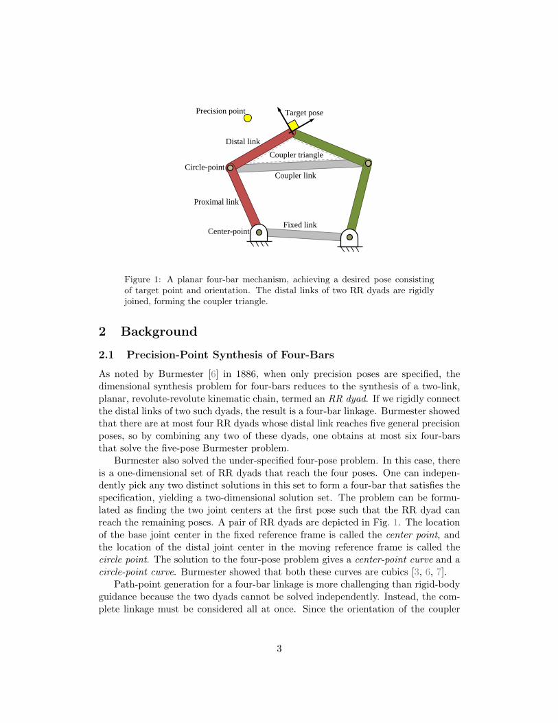
Figure 1: A planar four-bar mechanism, achieving a desired pose consistingof target point and orientation. The distal links of two RR dyads are rigidlyjoined, forming the coupler triangle.

2 Background

2.1 Precision-Point Synthesis of Four-Bars

As noted by Burmester [6] in 1886, when only precision poses are specified, thedimensional synthesis problem for four-bars reduces to the synthesis of a two-link,planar, revolute-revolute kinematic chain, termed an RR dyad. If we rigidly connectthe distal links of two such dyads, the result is a four-bar linkage. Burmester showedthat there are at most four RR dyads whose distal link reaches five general precisionposes, so by combining any two of these dyads, one obtains at most six four-barsthat solve the five-pose Burmester problem.

Burmester also solved the under-specified four-pose problem. In this case, thereis a one-dimensional set of RR dyads that reach the four poses. One can indepen-dently pick any two distinct solutions in this set to form a four-bar that satisfies thespecification, yielding a two-dimensional solution set. The problem can be formu-lated as finding the two joint centers at the first pose such that the RR dyad canreach the remaining poses. A pair of RR dyads are depicted in Fig. 1. The locationof the base joint center in the fixed reference frame is called the center point, andthe location of the distal joint center in the moving reference frame is called thecircle point. The solution to the four-pose problem gives a center-point curve and acircle-point curve. Burmester showed that both these curves are cubics [3, 6, 7].

Path-point generation for a four-bar linkage is more challenging than rigid-bodyguidance because the two dyads cannot be solved independently. Instead, the com-plete linkage must be considered all at once. Since the orientation of the coupler

3

link at precision points is not prescribed, there is greater freedom in the synthesisproblem. There are two center points and two circle points to be determined at theinitial precision point, for a total of eight unknown coordinates. Hence, includingthe initial point in the count the maximum number of precision path-points thatcan be generally prescribed is nine, a fact first observed by Alt [8].

When fewer than nine points are given, one may impose additional constraintson other aspects of the design. Depending on what kind of extra constraints are im-posed, one may pose a wide variety of synthesis problems such that a finite number ofsolutions are expected. Often, the constraints are chosen to most conveniently sim-plify the problem, and alternatively they might be chosen to meet design constraints,such as limits on where the base joint can be located. Among the various possiblecombinations of design constraints, Freudenstein and Sandor [9] developed a closedform solution for certain 2, 3 and 4 path-point problems. Suh and Radcliffe [10]developed a method that leads to a set of simultaneous nonlinear equations, whichcan be numerically solved for up to 5 path-points. Morgan and the last author [11]used continuation methods to develop solutions for the problem of 5 path-pointswith the center points prescribed. The full 9 path-point problem was attacked withheuristic continuation approaches in [12] and [13] to produce partial solution lists,while the first complete solution was reported in [14] using a rigorous continuationformulation. That work showed that for 9 generic path-points there are a total of4326 distinct four-bar solutions, which appear as 1442 triples of Roberts cognates.

In this article, we consider “mixed Burmester” synthesis problems in which amixture of M precision poses and N precision points are given. We shall refer toany one of these as an “M pose N point problem” or simply the “(M,N) problem”.Problems of this type were first posed in [5] along with some preliminary numericalresults obtained using polynomial continuation. The work reported here gives amore complete treatment of this family of problems.

2.2 Numerical Algebraic Geometry

One approach that has a long record of solving problems in kinematics is poly-nomial continuation. Some highlights in this history are Tsai and Morgan’s earlydemonstration that the inverse kinematics problem for general six-revolute robotshas 16 solutions [15], Raghavan’s demonstration that the forward kinematics ofgeneral Stewart-Gough platforms has 40 solutions [16], and, most relevant to thecurrent discussion, the first complete solution of the nine-precision-point problemfor four-bar synthesis [14].

All of the examples just cited are problems where a finite number of solutionsare expected. Subsequently, polynomial continuation has been extended to includemethods for dealing with polynomial systems that may have higher dimensionalsolution sets, such as curves, surfaces, and so on. The term numerical algebraicgeometry has been adopted to more accurately describe the current capabilities.Papers discussing these methods as a general approach to kinematics include [17, 18]

4

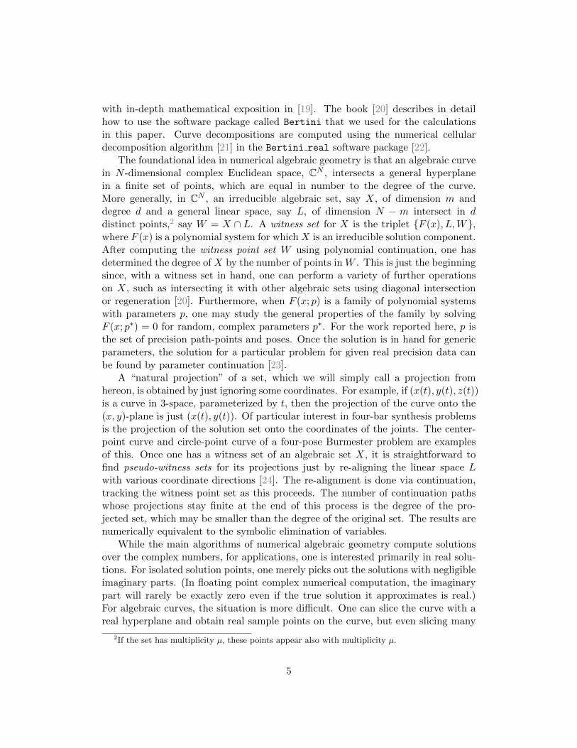
with in-depth mathematical exposition in [19]. The book [20] describes in detailhow to use the software package called Bertini that we used for the calculationsin this paper. Curve decompositions are computed using the numerical cellulardecomposition algorithm [21] in the Bertini real software package [22].

The foundational idea in numerical algebraic geometry is that an algebraic curvein N -dimensional complex Euclidean space, CN , intersects a general hyperplanein a finite set of points, which are equal in number to the degree of the curve.More generally, in CN , an irreducible algebraic set, say X, of dimension m anddegree d and a general linear space, say L, of dimension N − m intersect in ddistinct points,2 say W = X ∩ L. A witness set for X is the triplet {F (x), L,W},where F (x) is a polynomial system for which X is an irreducible solution component.After computing the witness point set W using polynomial continuation, one hasdetermined the degree of X by the number of points in W . This is just the beginningsince, with a witness set in hand, one can perform a variety of further operationson X, such as intersecting it with other algebraic sets using diagonal intersectionor regeneration [20]. Furthermore, when F (x; p) is a family of polynomial systemswith parameters p, one may study the general properties of the family by solvingF (x; p∗) = 0 for random, complex parameters p∗. For the work reported here, p isthe set of precision path-points and poses. Once the solution is in hand for genericparameters, the solution for a particular problem for given real precision data canbe found by parameter continuation [23].

A “natural projection” of a set, which we will simply call a projection fromhereon, is obtained by just ignoring some coordinates. For example, if (x(t), y(t), z(t))is a curve in 3-space, parameterized by t, then the projection of the curve onto the(x, y)-plane is just (x(t), y(t)). Of particular interest in four-bar synthesis problemsis the projection of the solution set onto the coordinates of the joints. The center-point curve and circle-point curve of a four-pose Burmester problem are examplesof this. Once one has a witness set of an algebraic set X, it is straightforward tofind pseudo-witness sets for its projections just by re-aligning the linear space Lwith various coordinate directions [24]. The re-alignment is done via continuation,tracking the witness point set as this proceeds. The number of continuation pathswhose projections stay finite at the end of this process is the degree of the pro-jected set, which may be smaller than the degree of the original set. The results arenumerically equivalent to the symbolic elimination of variables.

While the main algorithms of numerical algebraic geometry compute solutionsover the complex numbers, for applications, one is interested primarily in real solu-tions. For isolated solution points, one merely picks out the solutions with negligibleimaginary parts. (In floating point complex numerical computation, the imaginarypart will rarely be exactly zero even if the true solution it approximates is real.)For algebraic curves, the situation is more difficult. One can slice the curve with areal hyperplane and obtain real sample points on the curve, but even slicing many

2If the set has multiplicity µ, these points appear also with multiplicity µ.

5

times, one might miss interesting parts of the curve. There also can be ambiguityin how the points should connect to form the complete curve. A more secure, albeitmore costly, treatment is to form equations for sweeping a real slicing plane parallelto itself and to solve for all the critical points where the plane touches the curvetangentially [21]. These critical points include all the places where the real curvestarts, stops, or crosses itself, and if they exist, even finds isolated real points onthe complex curve. Between these critical points, the real arcs of the curve can beparametrized nonsingularly with respect to the sweeping coordinate, so they can besampled numerically to any desired resolution.

3 Formulation of the (M,N) Mixed Burmester Problem

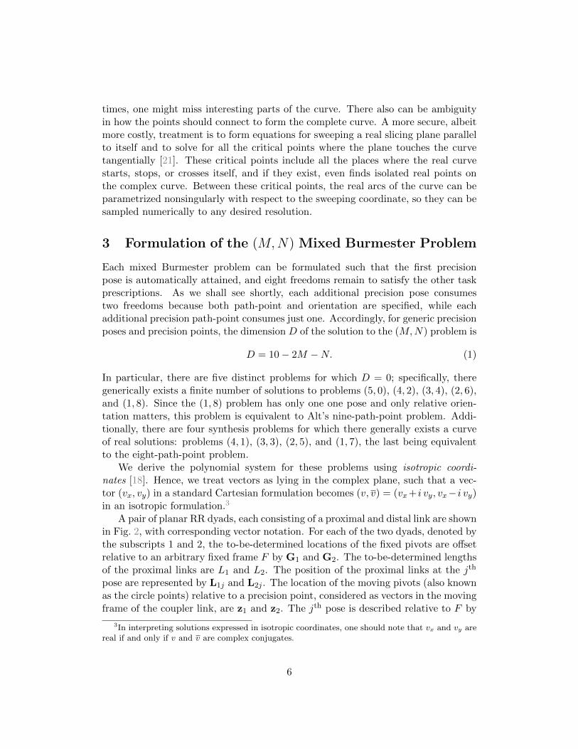
Each mixed Burmester problem can be formulated such that the first precisionpose is automatically attained, and eight freedoms remain to satisfy the other taskprescriptions. As we shall see shortly, each additional precision pose consumestwo freedoms because both path-point and orientation are specified, while eachadditional precision path-point consumes just one. Accordingly, for generic precisionposes and precision points, the dimension D of the solution to the (M,N) problem is

D = 10− 2M −N. (1)

In particular, there are five distinct problems for which D = 0; specifically, theregenerically exists a finite number of solutions to problems (5, 0), (4, 2), (3, 4), (2, 6),and (1, 8). Since the (1, 8) problem has only one one pose and only relative orien-tation matters, this problem is equivalent to Alt’s nine-path-point problem. Addi-tionally, there are four synthesis problems for which there generally exists a curveof real solutions: problems (4, 1), (3, 3), (2, 5), and (1, 7), the last being equivalentto the eight-path-point problem.

We derive the polynomial system for these problems using isotropic coordi-nates [18]. Hence, we treat vectors as lying in the complex plane, such that a vec-tor (vx, vy) in a standard Cartesian formulation becomes (v, v) = (vx+ i vy, vx− i vy)in an isotropic formulation.3

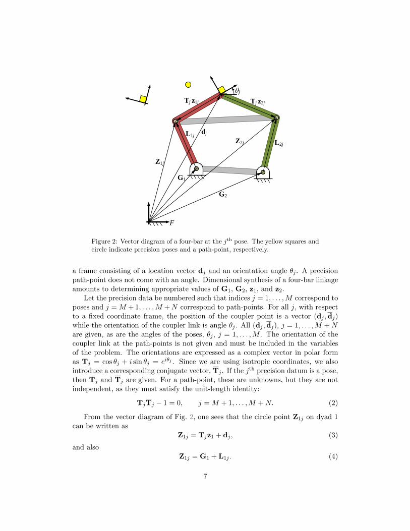
A pair of planar RR dyads, each consisting of a proximal and distal link are shownin Fig. 2, with corresponding vector notation. For each of the two dyads, denoted bythe subscripts 1 and 2, the to-be-determined locations of the fixed pivots are offsetrelative to an arbitrary fixed frame F by G1 and G2. The to-be-determined lengthsof the proximal links are L1 and L2. The position of the proximal links at the jth

pose are represented by L1j and L2j . The location of the moving pivots (also knownas the circle points) relative to a precision point, considered as vectors in the movingframe of the coupler link, are z1 and z2. The jth pose is described relative to F by

3In interpreting solutions expressed in isotropic coordinates, one should note that vx and vy arereal if and only if v and v are complex conjugates.

6

j

dj L1j

G1

Z1j

F

Tj z1j

L2j

Tj z2j

G2

Z2j

Figure 2: Vector diagram of a four-bar at the jth pose. The yellow squares andcircle indicate precision poses and a path-point, respectively.

a frame consisting of a location vector dj and an orientation angle θj . A precisionpath-point does not come with an angle. Dimensional synthesis of a four-bar linkageamounts to determining appropriate values of G1, G2, z1, and z2.

Let the precision data be numbered such that indices j = 1, . . . ,M correspond toposes and j = M + 1, . . . ,M +N correspond to path-points. For all j, with respectto a fixed coordinate frame, the position of the coupler point is a vector (dj ,dj)while the orientation of the coupler link is angle θj . All (dj ,dj), j = 1, . . . ,M +Nare given, as are the angles of the poses, θj , j = 1, . . . ,M . The orientation of thecoupler link at the path-points is not given and must be included in the variablesof the problem. The orientations are expressed as a complex vector in polar formas Tj = cos θj + i sin θj = eiθj . Since we are using isotropic coordinates, we alsointroduce a corresponding conjugate vector, Tj . If the jth precision datum is a pose,then Tj and Tj are given. For a path-point, these are unknowns, but they are notindependent, as they must satisfy the unit-length identity:

TjTj − 1 = 0, j = M + 1, . . . ,M +N. (2)

From the vector diagram of Fig. 2, one sees that the circle point Z1j on dyad 1can be written as

Z1j = Tjz1 + dj , (3)

and alsoZ1j = G1 + L1j . (4)

7

Combining these and writing the corresponding equation for the conjugate, we have,for j = 1, . . . ,M +N ,

L1j = Tjz1 + dj −G1, (5)

L1j = Tjz1 + dj −G1. (6)

The fundamental synthesis equation guarantees that the length of the proximal linkremains constant at all times. That is, for j = 2, . . . ,M +N ,

L1jL1j − L11L11 = 0. (7)

Similar equations can be formulated for the second RR dyad, which forms a secondset of synthesis equations, these being, for j = 1, . . . ,M +N ,

L2j = Tjz2 + dj −G2, (8)

L2j = Tjz2 + dj −G2, (9)

along with, for j = 2, . . . ,M +N ,

L2jL2j − L21L21 = 0. (10)

An accounting of the unknowns is as follows. In isotropic coordinates, the vectordescription of the linkage at the first precision datum has 8 variables, namely G1, G2,z1, z2 and their conjugates, G1, G2, z1, z2. Additionally, for each pose and path-point, we have unknowns L1j ,L2j and their conjugates L1j ,L2j . Finally, for N path-points, the rotation coordinates (Tj ,Tj) are unknown. This gives 8+4(M+N)+2Nunknowns in total.

An accounting of the equations is as follows: Eq. (2), for j = M + 1, . . . ,M +N ;Eqs. (5),(6),(8),(9), for j = 1, . . . ,M +N ; and Eqs. (7),(10), for j = 2, . . . ,M +N .For general precision data, the expected dimension of the solution set for the (M,N)mixed Burmester problem is the total number of variables minus the total numberof equations, which is 10− 2M −N as in (1).

Some simplifications can be performed which leave the expected dimension of thesolution set unchanged. For example, Eqs (5),(6),(8),(9) can be used to eliminateL1j , L2j , L1j , L2j from Eqs. (7),(10). This reduces the number of unknowns andequations both by 4(M +N).

4 Complete solution of the (M,N) problem

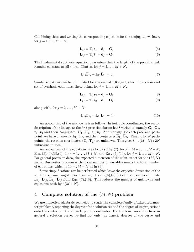
We use numerical algebraic geometry to study the complete family of mixed Burmes-ter problems, reporting the degree of the solution set and the degree of its projectionsonto the center point and circle point coordinates. For the four cases that have ingeneral a solution curve, we find not only the generic degrees of the curve and

8

its center-point and circle-point projections but also the generic number of criticalpoints of these curves. These indicate how many times the curve might reversedirection, which is a crucial step in plotting a curve. Section 5 considers a fewparticular examples of these curves and illustrate them with plots.

Although we solve the problems using a complete set of variables, namely

{G1,G2, z1, z2,G1,G2, z1, z2, [(Tj ,Tj), j = M + 1, . . . ,M +N ]},

we report on the degree of its projection onto the eight “natural” variables

{G1,G2, z1, z2,G1,G2, z1, z2}.

In the (M,N) combinations that give a zero-dimensional solution set, this degree isan upper bound on the number of real solutions that any problem in that class canhave. The degree of the projections of the solution set onto just the center pointcoordinates of dyad 1, (G1,G1), and separately onto just the circle point coordinatesof that dyad, (z1, z1), are often less than that of the original set.

4.1 Dimension and degree of the solution set

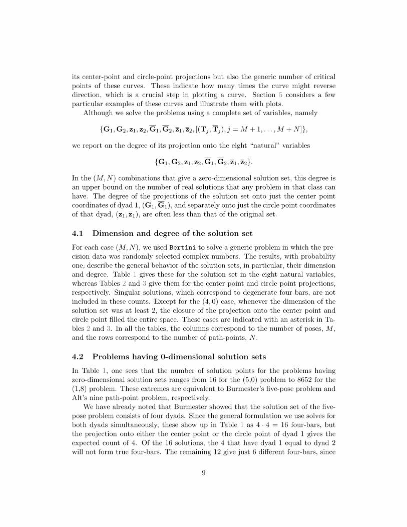
For each case (M,N), we used Bertini to solve a generic problem in which the pre-cision data was randomly selected complex numbers. The results, with probabilityone, describe the general behavior of the solution sets, in particular, their dimensionand degree. Table 1 gives these for the solution set in the eight natural variables,whereas Tables 2 and 3 give them for the center-point and circle-point projections,respectively. Singular solutions, which correspond to degenerate four-bars, are notincluded in these counts. Except for the (4, 0) case, whenever the dimension of thesolution set was at least 2, the closure of the projection onto the center point andcircle point filled the entire space. These cases are indicated with an asterisk in Ta-bles 2 and 3. In all the tables, the columns correspond to the number of poses, M ,and the rows correspond to the number of path-points, N .

4.2 Problems having 0-dimensional solution sets

In Table 1, one sees that the number of solution points for the problems havingzero-dimensional solution sets ranges from 16 for the (5,0) problem to 8652 for the(1,8) problem. These extremes are equivalent to Burmester’s five-pose problem andAlt’s nine path-point problem, respectively.

We have already noted that Burmester showed that the solution set of the five-pose problem consists of four dyads. Since the general formulation we use solves forboth dyads simultaneously, these show up in Table 1 as 4 · 4 = 16 four-bars, butthe projection onto either the center point or the circle point of dyad 1 gives theexpected count of 4. Of the 16 solutions, the 4 that have dyad 1 equal to dyad 2will not form true four-bars. The remaining 12 give just 6 different four-bars, since

9

Table 1: Dimension and degree of mixed Burmester solution sets, projectedonto all eight natural variables.

M1 2 3 4 5

N

0 8 1 6 4 4 16 2 16 0 161 7 7 5 24 3 64 1 482 6 43 4 134 2 194 0 603 5 234 3 552 1 3624 4 1108 2 1554 0 4025 3 3832 1 23886 2 8716 0 22247 1 108588 0 8652

Table 2: Dimension and degree of mixed Burmester solution sets, projectedonto the center point coordinates, (G1,G1).

M1 2 3 4 5

N

0 ∗ ∗ ∗ 1 3 0 41 ∗ ∗ ∗ 1 32 ∗ ∗ ∗ 0 603 ∗ ∗ 1 1284 ∗ ∗ 0 4025 ∗ 1 8166 ∗ 0 22247 1 35008 0 4326

switching the numbering on the two dyads counts as a different solution to thepolynomial system but makes no difference to the four-bar.

The other extreme, Alt’s (1, 8) problem, also shows a difference in degree amongstthe three tables, but this time only the center-point projection is lower. As was ob-served in [14], the 8652 solutions of this problem appear with two symmetry actions:they appear in triplets according to Roberts cognates and each of these appears twicejust by reversing the numbering of the two dyads. Thus, there are only 4326 distinctfour-bars, appearing as 1442 Roberts cognate triplets. However, it is known thatthe center points of a Roberts cognate triplet form a triangle similar to the coupler

10

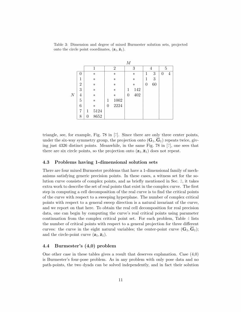
Table 3: Dimension and degree of mixed Burmester solution sets, projectedonto the circle point coordinates, (z1, z1).

M1 2 3 4 5

N

0 ∗ ∗ ∗ 1 3 0 41 ∗ ∗ ∗ 1 32 ∗ ∗ ∗ 0 603 ∗ ∗ 1 1424 ∗ ∗ 0 4025 ∗ 1 10026 ∗ 0 22247 1 51248 0 8652

triangle, see, for example, Fig. 78 in [7]. Since there are only three center points,under the six-way symmetry group, the projection onto (G1,G1) repeats twice, giv-ing just 4326 distinct points. Meanwhile, in the same Fig. 78 in [7], one sees thatthere are six circle points, so the projection onto (z1, z1) does not repeat.

4.3 Problems having 1-dimensional solution sets

There are four mixed Burmester problems that have a 1-dimensional family of mech-anisms satisfying generic precision points. In these cases, a witness set for the so-lution curve consists of complex points, and as briefly mentioned in Sec. 2, it takesextra work to describe the set of real points that exist in the complex curve. The firststep in computing a cell decomposition of the real curve is to find the critical pointsof the curve with respect to a sweeping hyperplane. The number of complex criticalpoints with respect to a general sweep direction is a natural invariant of the curve,and we report on that here. To obtain the real cell decomposition for real precisiondata, one can begin by computing the curve’s real critical points using parametercontinuation from the complex critical point set. For each problem, Table 4 liststhe number of critical points with respect to a general projection for three differentcurves: the curve in the eight natural variables; the center-point curve (G1,G1);and the circle-point curve (z1, z1).

4.4 Burmester’s (4,0) problem

One other case in these tables gives a result that deserves explanation. Case (4,0)is Burmester’s four-pose problem. As in any problem with only pose data and nopath-points, the two dyads can be solved independently, and in fact their solution

11

Table 4: Numbers of critical points for all one-dimensional mixed Burmesterproblems with respect to polynomial system from Sec. 3.

(M,N) Generic number of critical points

All 8 natural variables (G1,G1) (z1, z1)

(1, 7) 55676 4168 38740 4168 44208 4168(2, 5) 11228 988 8084 988 8456 988(3, 3) 1440 144 972 144 1000 144(4, 1) 152 16 92 16 92 16

nonsingular singular nonsingular singular nonsingular singular

sets are identical. Due to this independence, when projected onto either the centerpoint or the circle point coordinates, the two-dimensional solution set of case (4,0)becomes just one-dimensional. As shown in Tables 2 and 3, the center-point curveand the circle-point curve are each cubics, as was found by Burmester long ago.

Any problem of type (M, 0) should be solved taking advantage of the Burmester’stechnique of separating the two dyads. We report the results for these cases usingthe general formulation only for completeness.

5 Examples

The following present three examples of solving mixed Burmester problems. Allcomputations were done using Bertini to obtain solution points or witness setsand Bertini real to extract real curves.

5.1 0-dimensional solution set – a (4, 2) problem

The (4, 2) problem has a zero dimensional solution set for generic parameter values.Table 5 contains randomly chosen values for the poses and points, which are usedfor the discussion here.

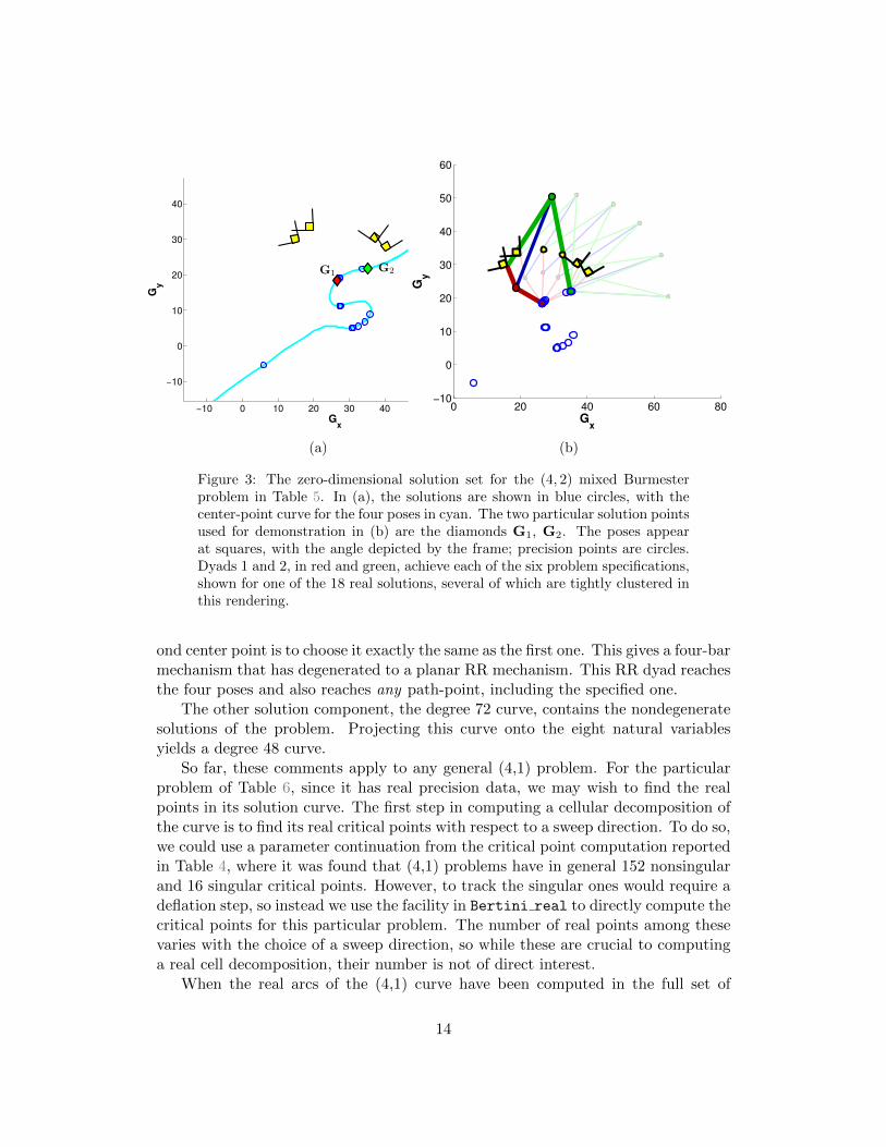
The problem has 60 complex solutions, of which 18 are real. The center pointsof the solutions must lie on the center-point curve of the associated (4, 0) problemobtained by dropping the two path-points. In Fig. 3(a), the locations of the centerpoints for the (4,2) problem are shown superimposed on the center-point curve ofthe (4,0) problem, along with the four poses. Picking any one of the center points fordyad 1 automatically picks a corresponding center point for dyad 2 from the sameset, thus the 18 center points correspond to just 9 distinct four-bar solutions. These18 solutions are closely clustered in projection onto the center point. In Fig. 3(b),we show how one of the solutions achieves the four poses and two path-points.

12

Table 5: Mixed Burmester task consisting of 4 poses and 2 path-points

j djx djy θj (deg)

1 15.95 29.38 102.072 19.84 32.66 91.723 26.90 34.41 –4 32.66 32.93 –5 37.40 29.06 53.526 40.00 26.59 30.45

5.2 1-dimensional solution set – a (4, 1) problem

The (4, 1) mixed Burmester problem generically has a 1-dimensional solution set offour-bar linkages. Table 6 gives specific parameter values we use in this example.

Table 6: Task specification with four poses and one point

j djx djy θj (deg)

1 22.13 11.54 -24.152 20.98 22.88 6.933 10.45 23.44 –4 5.23 27.17 54.145 -5.66 24.14 78.02

Computing a numerical irreducible decomposition using Bertini reveals thatthe algebraic variety in all of the variables for any (4,2) problem has two irreduciblecomponents of dimension one: one of degree 16 and the other of degree 72. As wewill explain, the degree 16 piece is degenerate, so we ignore it. The degree 72 pieceprojects to a degree 48 curve in the eight natural variables, so this is the numberreported in Table 1. Both components are self-conjugate, and hence potentiallycontain real curves.

As in the (4,2) case, the results for the (4,1) case can be better understood byconsidering the center-point curve of the associated (4,0) problem. This time, the(4,1) problem has a solution curve and it projects to exactly cover the (4,0) center-point curve. But the (4,1) problem and the associated (4,0) problem do not havethe same solution set. The difference is that for the (4,0) problem, one can pick anytwo points on the center-point curve to form a four-bar. For the (4,1) problem, thechoice for one center point must be matched by one of a finite set of center pointsfor the other dyad such that the resulting four-bar will reach the extra path-point.

The degenerate degree 16 component occurs because one possibility for the sec-

13

−10 0 10 20 30 40 50 60

−10

0

10

20

30

40

Gx

Gy

(a)

0 20 40 60 80−10

0

10

20

30

40

50

60

Gx

Gy

(b)

Figure 3: The zero-dimensional solution set for the (4, 2) mixed Burmesterproblem in Table 5. In (a), the solutions are shown in blue circles, with thecenter-point curve for the four poses in cyan. The two particular solution pointsused for demonstration in (b) are the diamonds G1, G2. The poses appearat squares, with the angle depicted by the frame; precision points are circles.Dyads 1 and 2, in red and green, achieve each of the six problem specifications,shown for one of the 18 real solutions, several of which are tightly clustered inthis rendering.

ond center point is to choose it exactly the same as the first one. This gives a four-barmechanism that has degenerated to a planar RR mechanism. This RR dyad reachesthe four poses and also reaches any path-point, including the specified one.

The other solution component, the degree 72 curve, contains the nondegeneratesolutions of the problem. Projecting this curve onto the eight natural variablesyields a degree 48 curve.

So far, these comments apply to any general (4,1) problem. For the particularproblem of Table 6, since it has real precision data, we may wish to find the realpoints in its solution curve. The first step in computing a cellular decomposition ofthe curve is to find its real critical points with respect to a sweep direction. To do so,we could use a parameter continuation from the critical point computation reportedin Table 4, where it was found that (4,1) problems have in general 152 nonsingularand 16 singular critical points. However, to track the singular ones would require adeflation step, so instead we use the facility in Bertini real to directly compute thecritical points for this particular problem. The number of real points among thesevaries with the choice of a sweep direction, so while these are crucial to computinga real cell decomposition, their number is not of direct interest.

When the real arcs of the (4,1) curve have been computed in the full set of

14

−30 −20 −10 0 10 20 30 40

−20

−10

0

10

20

30

40

Gx

Gy

Figure 4: A projection of the solution curve for the (4, 1) mixed Burmester ex-ample problem. There is an interval where no mechanism may be constructed.

coordinates, the curve can be drawn in any projection. Fig. 4 shows the projectiononto the center-point coordinates. Curiously, although the entire (4,1) solution curveprojects to cover the entirety of the related (4,0) center-point curve, the real pointsof the (4,1) curve do not cover all the real points of the (4,0) center-point curve;as seen in the figure, there is a gap. This surprising fact has a straightforwardexplanation: in the gap, there are real points of the (4,0) curve that reach all fourposes, but to reach the specified path-point, the coupler link must take a non-realrotation angle.

In all cases observed, the boundary points of the gap were associated with theRR dyad reaching the end of its workspace (i.e., the proximal and distal links havebecome parallel). Thus, L1j is parallel to Tjz1, which is expressed as

Tjz1L1j −Tjz1L1j = 0. (11)

Linkages that are at the edge of the workspace can be found by adding Eq. (11) tothe synthesis constraints of Eqs. (2), (7) and (10). After solving the system, valuesof G corresponded with each gap boundary on the (4,1) curve.

5.3 1-dimensional solution set – a (3, 3) problem

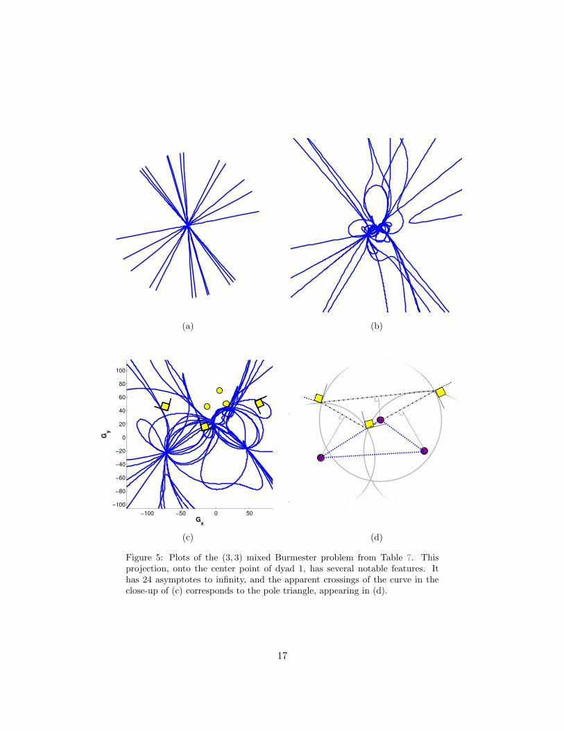
As a final example, we consider synthesizing a four-bar mechanism to guide arigid body through the 3 task poses and 3 path-points given in Table 7. UsingBertini real, we computed a cellular decomposition of the solution curve. Theprojection of this curve onto the center-point plane is shown in Fig. 5. Accordingto Table 2, this projection is a curve of degree 128, while Table 4 gives the genericnumber of critical points in the different projections we have been discussing. Sim-ilar to the (4,1) problem, picking one center point G1 from this curve determines afinite number of locations for the other center point, G2. These points must also lieon this same center-point curve.

15

Table 7: Task combination with 3-poses and 3-points

j djx djy θj1 -72.67 39.91 72.512 -20.22 10.00 15.213 57.82 53.08 -63.514 5.06 70.00 –5 -13.32 46.20 –6 15.22 50.28 –

Figure 5 shows the center-point curve at three different scales. Zoomed far out,Fig. 5a accentuates the asymptotes to infinity of the curve. These appear as 12asymptotes, defining 24 rays. A center-point at infinity means that the associatedcircle point moves on a circle of infinite radius, which makes these points equiva-lent to a slider joint. In this way, we see that the solution set for the particular(3,3) problem under consideration includes 12 PRRR-type four-bars. One could, ofcourse, set up a new problem to solve for these directly: a mixed Burmester (3,3)problem for slider-cranks.

Zooming in twice produces Figs. 5b and 5c that show more details of the curve.Especially in Fig. 5c, one may notice that there are three points in the plane wherethe center-point curve has multiple self-crossings. Further investigation shows thatthese points seem to be related to the three precision poses and are not dependent onthe three path-points. In particular, the self-crossings coincide with the poles of thethree poses. This is illustrated in Fig. 5d, which shows just the three precision posesand their poles. At present, we have no further explanation for this phenomenon,but we conjecture that the center-point curve of any (3,3) mixed Burmester problemhas self-crossings at the vertices of the related pole triangle.

6 Conclusions

We have studied all the mixed (M,N) Burmester problems using numerical algebraicgeometry as implemented in the Bertini software package. We give the dimensionand degree of the solution set for every general case from the trivial (1,0) problemthat has an 8-dimensional solution, up to the five cases that have 0-dimensionalsolutions. The 0-dimensional cases, which include Burmester’s five-pose problem,case (5,0), and Alt’s nine path-point problem, case (1,8), have degrees ranging from16 to 8652. Those extremes had been settled before, but the mixed cases in between,namely (4,2), (3,4), and (2,6), are newly treated. The four cases with solutioncurves have been investigated in more depth to the extent of determining the generalnumber of critical points of each, a step that is useful in plotting the real arcs of

16

(a)

(b)

−100 −50 0 50

−100

−80

−60

−40

−20

0

20

40

60

80

100

Gx

Gy

(c) (d)

Figure 5: Plots of the (3, 3) mixed Burmester problem from Table 7. Thisprojection, onto the center point of dyad 1, has several notable features. Ithas 24 asymptotes to infinity, and the apparent crossings of the curve in theclose-up of (c) corresponds to the pole triangle, appearing in (d).

17

these curves. The (1,7) curve is the most difficult one in the set, having, in thenatural 8 coordinates, a degree of 10,858 and approximately five times that numberof critical points. For the more tractable cases of the (4,1) and (3,3) problems, wegive illustrations of the center-point curves for a specific example of each and pointout interesting features of these.

7 Acknowledgments

DAB and JDH were supported in part by DARPA Young Faculty Award, NSFACI-1460032, and Sloan Research Fellowship. CWW was supported in part by NSFACI-1440607.

References

[1] Erdman, A., Sandor, G., and Kota, S., 2001, Mechanism Design: Analysis andSynthesis, Vol. 1, 4/e, Prentice-Hall, Englewood Cliffs, NJ.

[2] McCarthy, J.M., and Soh, G.S., 2011, Geometric Design of Linkages, 2/e,Springer-Verlag, New York.

[3] Sandor, G., Erdman, A., 1984, Advanced Mechanism Design: Analysis andSynthesis, Vol. 2, Prentice-Hall, Englewood Cliffs, NJ.

[4] Balli, S.S. and Chand, S., 2002, “Defects in Link Mechanisms and SolutionRectification”, Mech. Mach. Theory, 37(9), pp. 851-876.

[5] Tong, Y., Myszka, D.H., and Murray, A.P., 2013, “Four-Bar Linkage Synthe-sis for a Combination of Motion and Path-Point Generation”, Proceedings ofthe ASME International Design Engineering Technical Conferences, Paper No.DETC2013-12969.

[6] Burmester, L., 1886, Lehrbuch der Kinematic, Verlag Von Arthur Felix, Leipzig,Germany.

[7] Bottema, O., and Roth, B., 1990, Theoretical Kinematics, Dover Publications,Mineola, NY.

[8] Alt, H., 1923, “Uber die Erzeugung gegebener ebener Kurven mit Hilfe desGelenkvierecks”, ZAMM, 3(1), pp. 13–19.

[9] Freudenstein, F. and Sandor, G., 1959, “Synthesis of Path Generating Mech-anisms by Means of a Programmed Digital Computer”, ASME J. Eng. Ind.,81(1), pp. 159–168.

18

[10] Suh, C. and Radcliffe, C., 1966, “Synthesis of Path Generating Mechanismswith Use of the Displacement Matrix”, Proceedings of the ASME InternationalDesign Technical Conferences, 66-MECH-19, pp. 9-19.

[11] Morgan, A. and Wampler, C., 1990, “Solving a Planar Fourbar Design ProblemUsing Continuation”, ASME J. Mech. Des., 112(4), pp. 544-550.

[12] Roth, B., and Freudenstein, F., 1963, “Synthesis of Path-Generating Mecha-nisms by Numerical Means”, ASME J. Eng. Ind., 85(3), pp. 298–306.

[13] Tsai, L.-W., and Lu, J.-J., 1989, “Coupler-Point-Synthesis Using HomotopyMethods”, Advances in Design Automation—1989: Mechanical Systems Anal-ysis, Design and Simulation, B. Ravani, ed., ASME DE-Vol. 19-3, pp. 417–424.

[14] Wampler, C.W., 1992, “Complete Solution of the Nine-Point Path SynthesisProblem for Fourbar Linkages”, ASME J. Mech. Des., 114(1), pp. 153-161.

[15] Tsai, L.W. and Morgan, A.P., 1985, “Solving the Kinematics of the Most Gen-eral Six- and Five-Degree-of-Freedom Manipulators by Continuation Methods”,ASME J. Mech., Trans., Automation, 107(2), pp. 189–200.

[16] Raghavan, M., 1993, “The Stewart Platform of General Geometry has 40 Con-figurations”, ASME J. Mech. Des., 115(2), pp. 277–282.

[17] Sommese, A.J., Verschelde, J., and Wampler, C.W., 2004, “Advances in Poly-nomial Continuation for Solving Problems in Kinematics”, ASME J. Mech.Des., 126(2), pp. 262–268.

[18] Wampler, C.W., and Sommese, A.J., 2011, “Numerical Algebraic Geometryand Algebraic Kinematics”, Acta Numerica, 20, pp. 469–567.

[19] Sommese, A.J., and Wampler, C.W., 2005, Numerical Solution of Systems ofPolynomials Arising In Engineering And Science, World Scientific Press, Sin-gapore.

[20] Bates, D.J., Hauenstein, J.D., Sommese, A.J., and Wampler, C.W., 2013, Nu-merically Solving Polynomial Systems with Bertini, Software, Environments,and Tools 25, SIAM, Philadelphia, PA. Software available at bertini.nd.edu.

[21] Lu, Y., Bates, D.J., Sommese, A.J., and Wampler, C.W., 2007, “Finding AllReal Points of a Complex Curve”, Contemp. Math. 448(8), pp. 183–205.

[22] Brake, D.A., Bates, D.J., Hao, W., Hauenstein, J.D., Sommese, A.J., andWampler, C.W., 2014, “Bertini real: Software for One- and Two-DimensionalReal Algebraic Sets”, Mathematical Software - ICMS 2014, Springer, pp. 175–182. Software available at bertinireal.com.

19

[23] Morgan, A.P., and Sommese, A.J., 1989, “Coefficient-Parameter PolynomialContinuation”, Appl. Math. Comput., 29(2), pp. 123–160. Errata, 1992, Appl.Math. Comput., 51, pp. 207.

[24] Hauenstein, J.D. and Sommese, A.J., 2010, “Witness Sets of Projections”,Appl. Math. Comput., 217(7), pp. 3349–3354.

20