the combination of circle topology and leaky integrator

RESEARCH ARTICLE

The combination of circle topology and leaky

integrator neurons remarkably improves the

performance of echo state network on time

series prediction

Fangzheng Xue1,2, Qian Li1,2, Xiumin Li1,2*

1 Key Laboratory of Dependable Service Computing in Cyber Physical Society of Ministry of Education,

Chongqing University, Chongqing 400044, China, 2 College of Automation, Chongqing University, Chongqing

400044, China

* [email protected]

Abstract

Recently, echo state network (ESN) has attracted a great deal of attention due to its high

accuracy and efficient learning performance. Compared with the traditional random struc-

ture and classical sigmoid units, simple circle topology and leaky integrator neurons have

more advantages on reservoir computing of ESN. In this paper, we propose a new model of

ESN with both circle reservoir structure and leaky integrator units. By comparing the predic-

tion capability on Mackey-Glass chaotic time series of four ESN models: classical ESN, cir-

cle ESN, traditional leaky integrator ESN, circle leaky integrator ESN, we find that our circle

leaky integrator ESN shows significantly better performance than other ESNs with roughly 2

orders of magnitude reduction of the predictive error. Moreover, this model has stronger

ability to approximate nonlinear dynamics and resist noise than conventional ESN and ESN

with only simple circle structure or leaky integrator neurons. Our results show that the com-

bination of circle topology and leaky integrator neurons can remarkably increase dynamical

diversity and meanwhile decrease the correlation of reservoir states, which contribute to the

significant improvement of computational performance of Echo state network on time series

prediction.

Introduction

Echo state network (ESN), one of the improved recurrent neural networks, has attracted exten-

sive attention since proposed by Jaeger in 2002 [1]. Unlike recurrent neural network, ESN has

a non-trainable sparse connected recurrent part (dynamic reservoir) as the hidden layer and

only the output weight need to be trained. The internal weights and input weights of ESN are

generated randomly and remain unchanged during training and testing. The readout training

is a simple linear regression problem for supervised learning. Due to the simple method and

high learning efficiency, ESN has been successfully applied to many fields, such as time series

PLOS ONE | https://doi.org/10.1371/journal.pone.0181816 July 31, 2017 1 / 17

a1111111111

a1111111111

a1111111111

a1111111111

a1111111111

OPENACCESS

Citation: Xue F, Li Q, Li X (2017) The combination

of circle topology and leaky integrator neurons

remarkably improves the performance of echo

state network on time series prediction. PLoS ONE

12(7): e0181816. https://doi.org/10.1371/journal.

pone.0181816

Editor: Zhong-Ke Gao, Tianjin University, CHINA

Received: July 2, 2016

Accepted: June 26, 2017

Published: July 31, 2017

Copyright: © 2017 Xue et al. This is an open access

article distributed under the terms of the Creative

Commons Attribution License, which permits

unrestricted use, distribution, and reproduction in

any medium, provided the original author and

source are credited.

Data Availability Statement: All relevant data are

within the paper and its Supporting Information

files.

Funding: This work is supported by the National

Natural Science Foundation of China (Nos.

61473051), Natural Science Foundation of

Chongqing (No. cstc2016jcyjA0015) and

Fundamental Research Funds for the Central

Universities (No. 106112017CDJXY170004). The

funders had no role in study design, data collection

and analysis, decision to publish, or preparation of

the manuscript.

https://doi.org/10.1371/journal.pone.0181816

http://crossmark.crossref.org/dialog/?doi=10.1371/journal.pone.0181816&domain=pdf&date_stamp=2017-07-31








http://creativecommons.org/licenses/by/4.0/

http://creativecommons.org/licenses/by/4.0/

prediction tasks [2, 3], dynamic pattern classification [4–7], telephone traffic forecasting [8, 9],

stock price prediction [10], speech recognition [11, 12], and so on.

Recently, many modified ESN models have been proposed from different aspects to

enhance the network performance: (1) From the reservoir topology perspective, literature [13]

successfully applied small-word network and scale-free network based on complex network

theory to replace the random dynamic reservoir topology of ESN; a new scale-free and highly

clustered ESN with both small-world feature and scale-free characteristic was proposed in [14,

15]; In [16] the authors adopted hierarchical reservoir to deal with multiscale input signal

based on the error gradient descent method and decoupled reservoirs were applied to ESN in

[17]. Contrary to a randomly initialized and fixed structure, [18, 19] used developmental self-

organization approaches to regulate the synaptic and structural plasticity of the dynamic reser-

voir according to the specific tasks. In addition, various methods have been proposed for ana-

lysing time series by means of complex network [20, 21]. It has been shown that these

approaches have advantage for characterizing real complex systems from nonlinear time series

[22–24]. These studies provide insights for constructing reservoir topology of ESNs. (2) In the

aspect of training algorithms, [25] applied ridge regression learning algorithm in ESN to solve

the ill-condition matrix; In [26], the authors proposed a priori data-driven multi-cluster reser-

voir generation algorithm; A regularized variational Bayesian learning was learned in [27]. (3)

In terms of reservoir neuron models, wavelet neurons were used in reservoir state update

equation in [28] and filter neurons were adopted in [29]. (4) From the point of energy con-

sumption, it has been found that the performance of network structure is not only related to

the weight of network connectivity, but also to the energy utilization of the network behavior

[30–33].

Specifically, in order to reduce the randomness of dynamical reservoir, a predefined singu-

lar value spectrum of the internal weight matrices is adopted in [34]. To further simplify the

reservoir topology, literature [35] put forward several simple topologies: delay line reservoir

(DLR), delay line reservoir with feedback connections (DLRB) and simple cycle reservoir

(SCR). These three reservoir construction approaches are simple and deterministic to realize

without the loss of performance compared to classical ESN for some learning tasks. To

increase the diversities of the dynamic reservoir, [28] injected wavelet neurons into reservoir

and assigned the sigmoid and wavelet neurons randomly. [36] replaced parts of sigmoid neu-

rons with wavelet units in a circle structure at different injecting ratio and distribution interval.

It has been proved that the hybrid circle reservoirs which contain two kinds of neurons have

certain advantages over the simple circle structures with only one kind of neuron.

In [1] and [12], Jaeger also proposed that the internal neurons were not confined to sigmoid

units and applied leaky integrator neurons to ESN. He pointed out some disadvantages pre-

senting traditional sigmoid neurons: (1) The conventional sigmoid units did not have a time

constant compared with the continuous leaky integrator neuron model; (2) The sigmoid units

are memoryless since the next time state values of reservoir units in standard sigmoid net-

works do not depend on their previous values directly. Thus, it is more appropriate for us to

apply the continuously and slowly changing systems using the continuous-time leaky integra-

tor network.

In general, although the influence of either circle topology or leaky integrate neuron on res-

ervoir computing have been studied in literature, the combined effect of these two factors have

not been considered and carefully analyzed. Therefore, in this paper we apply both the circle

structure and leaky integrator neuron to improve the computational performance of ESN,

motivated by leaky integrator ESN introduced in [37] and the simple circle topology. Mackey-

Glass time series is used to test the performance of four ESN networks: classical random ESN

with sigmoid neurons, circle ESN with sigmoid neurons, random ESN with leaky integrator

The combination of circle topology and leaky integrator neurons for ESN


Competing interests: The authors have declared

that no competing interests exist.


neurons, circle ESN with leaky integrator neurons. The prediction accuracy, nonlinear dynam-

ics approximation ability and anti-noise capability are investigated respectively. The results

show that our circle ESN with leaky integrator neurons remarkably outperform other ESNs.

This work provides an efficient model of ESN with excellent performance and simple network

structure, which is very meaningful for the broad application of ESN on various fields.

This paper is organized as follows. Section 2 describe four ESN models with different reser-

voir topology and neuron models. Section 3 briefly present experiment design including learn-

ing task, specific parameters setting and training process. Experiment results are shown in

section 4. Finally, discussion and conclusion are made in Section 5.

ESNS

Traditional echo state network

The architecture of ESN comprises an input layer, dynamical reservoir, and readout neuron.

The traditional ESN has a randomly connected reservoir as illustrated in Fig 1. The ESNs are

assumed to have K input neurons, N reservoir neurons, and L readout neurons, whose activa-

tion at time step n are denoted by u(n) = (u1(n), . . .uK(n))T, x(n) = (x1(n), . . .xN(n))T, and y(n)

= (y1(n), . . .yL(n))T, respectively (In the rest of the paper, vectors are denoted by boldface low-

ercase letters, e.g., a, while matrices are denoted by boldface uppercase letters, e.g., A). The

connection weights from the input neurons to reservoir neurons are given in a N × K matrix

Win. The reservoir connection weights are collected in a N × N weight matrix Wres. The con-

nection weights from the input and reservoir neurons to the readout neurons are given in a L× (K + N) matrix Wout. Furthermore, the connection weights projected back from the readout

neurons to the reservoir neurons are given in a N × L matrix Wback.

Fig 1. The regular echo state network model with random reservoir topology.

https://doi.org/10.1371/journal.pone.0181816.g001





The reservoir is updated according to the following equation:

xðnþ 1Þ ¼ f ðWinuðnþ 1Þ þWresxðnÞ þWbackyðnÞ þ vðnÞÞ; ð1Þ

where f is the activation function of the reservoir units (usually sigmoid function) and v(n) is a

noise, we use tanh function as the internal neurons function here. The output is computed as:

yðnþ 1Þ ¼ f outðWout½uðnþ 1Þjxðnþ 1Þ�Þ; ð2Þ

where fout denotes the activation function of the output neuron, [u(n + 1)|x(n + 1)] denotes the

concatenation vectors of the input and internal activation vectors and Wout is the output

weight matrix that has been trained. In our paper, we use tanh function as the readout function

as well.

In order to guarantee the echo state property (ESP), the spectral radius of the reservoir

weight matrix must be kept below 1. This can be achieved by scaling the initialized sparse

weight W0 into a new matrix Wres = k W0/|σmax|, where |σmax| denotes the spectral radius of

W0 and the value of the scaling parameter k belong to (0, 1).

ESNs with leaky integrator neurons

The traditional sigmoid units in reservoir have no working memory while the leaky integrator

neurons have. Therefore, it is more proper to choose the leaky integrator units for learning the

slowly and continuously changing dynamical systems. ESNs with leaky integrator neurons

which is called leaky integrator ESN (LI-ESN) has been reported in [38]. The dynamic equa-

tion of LI-ESN is similar to the model proposed by Jaeger [37] described as follows:

_x ¼1

zð� ax þ f ðWinuþWresx þWbacky þ vÞÞ; ð3Þ

where z> 0 is the time constant. The positive constant a is the leaky decay rate and f denotes

the activation function (we use sigmoid function as well). The matrix Win represents the input

weight matrix, Wres denotes the internal weight matrix, Wback is the feedback connection

weight matrix. u, x, y, v denote the input vector, the reservoir state vector, the output vector

and the noise vector, respectively. According to [39], the differential equation can be approxi-

mately turned into a difference equation as follows:

xðnþ 1Þ ¼ ð1 � aÞxðnÞ þ f ðWinuðnþ 1Þ þWresxðnÞ þWbackyðnÞ þ vðnÞÞ; ð4Þ

where x(n) denotes the internal state vector at the sample time step n. The training method is

similar to the classical ESN. The method for choosing the adequate parameter a will be dis-

cussed later.

ESNs with Low complexity circle reservoir topology

In this section, we introduce two ESNs with the simple circle reservoir topology shown in

Fig 2 with sigmoid or leaky integrator neurons, which are called circle ESN (C-ESN) and circle

LI-ESN (C-LI-ESN) respectively. Unlike the conventional ESN and LI-ESN, the input weight

matrix Win and the reservoir weight matrix Wres of C-ESN, C-LI-ESN have fixed weight values

of v and r. The matrix of cycle reservoir and input weight matrix are described in Eqs (5) and

(6), respectively. The values of v, r and a are adjusted depending on specific tasks. However,

the reservoir update equation and the training process are done in similar ways as classical




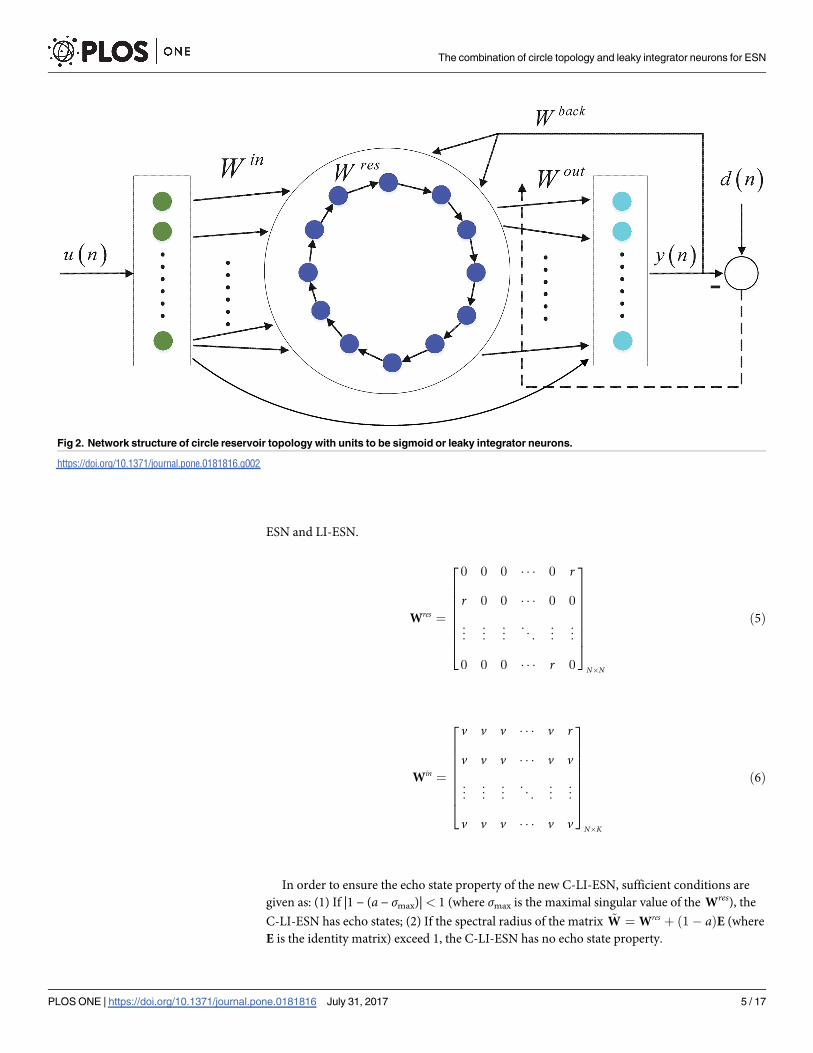
ESN and LI-ESN.

Wres ¼

0 0 0 � � � 0 r

r 0 0 � � � 0 0

..

. ... ..

. . .. ..

. ...

0 0 0 � � � r 0

2

66666664

3

77777775

N�N

ð5Þ

Win ¼

v v v � � � v r

v v v � � � v v

..

. ... ..

. . .. ..

. ...

v v v � � � v v

2

66666664

3

77777775

N�K

ð6Þ

In order to ensure the echo state property of the new C-LI-ESN, sufficient conditions are

given as: (1) If |1 − (a − σmax)|< 1 (where σmax is the maximal singular value of the Wres), the

C-LI-ESN has echo states; (2) If the spectral radius of the matrix ~W ¼Wres þ ð1 � aÞE (where

E is the identity matrix) exceed 1, the C-LI-ESN has no echo state property.

Fig 2. Network structure of circle reservoir topology with units to be sigmoid or leaky integrator neurons.






Experiment design

Learning task

In order to compare the performance of the four networks described above, we choose the

widely used learning task: the Mackey-Glass system (MGS) time series prediction [5]. The dis-

crete-time sequence equation of the MGS is defined as:

yðt þ 1Þ ¼ yðtÞ þ d0:2y t �

t

d

� �

1þ y t �t

d

� �10� 0:1yðtÞ

0

B@

1

CA; ð7Þ

where δ is the step size parameter which will always be set 0.1 with subsequently sub-sampling

by 10, τ denotes the time delay parameter which determines the nonlinearity degree of the

MGS. The MGS is a chaotic system if τ> 16.8. In this paper, two time series—one mild chaotic

system and another wild system with τ = 17 and τ = 30 respectively will be used for prediction

tasks. Fig 3 shows 1000-step subsequences of the two training sequences for these two cases.

Network preparation

In this paper, all of the four types of ESNs comprise one input unit, 200 reservoir units, and

one readout neuron. The input is a fixed signal u(n) = 0.02. The magnitude of the noise is set

1e-10. For the traditional ESN, weight matrices Win and Wback are drawn from a uniform dis-

tribution over [−1, 1], the spectral radius is set 0.85. For the circle topology structure and the

LI-ESN, the optimal values for the fixed weight values v, r of Win, Wres and the decay constant

a are considered as follows: 1) For LI-ESN, the matrix Wres is firstly re-scaled to 0.5 so that

σmax = 0.5; a is set 0.6 to ensure |1 − (a − σmax)|< 1 and the effective spectral radius of ~Wapproximates 0.85; the connection values of Win and Wback are the same as the traditional

ESN. 2) For C-ESN, the input connection parameter v is chosen as 0.1 and the reservoir weight

is 0.5 according to [36]. 3) For C-LI-ESN, we set the input weight v = 0.1 and reservoir weight

r = 0.5, where the maximum singular value of Wres equals 0.5. In order to guarantee the echo

state property, the decay constant a must be bigger than 0.5. In order to choose the optimal

Fig 3. The Macky-Glass time series with (a) τ = 17 and (b) τ = 30.






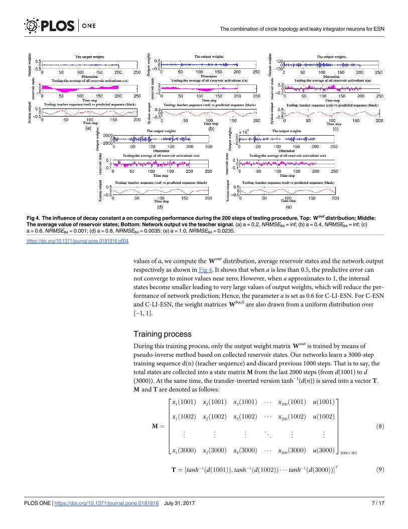
values of a, we compute the Wout distribution, average reservoir states and the network output

respectively as shown in Fig 4. It shows that when a is less than 0.5, the predictive error can

not converge to minor values near zero; However, when a approximates to 1, the internal

states become smaller leading to very large values of output weights, which will reduce the per-

formance of network prediction; Hence, the parameter a is set as 0.6 for C-LI-ESN. For C-ESN

and C-LI-ESN, the weight matrices Wback are also drawn from a uniform distribution over

[−1, 1].

Training process

During this training process, only the output weight matrix Wout is trained by means of

pseudo-inverse method based on collected reservoir states. Our networks learn a 3000-step

training sequence d(n) (teacher sequence) and discard previous 1000 steps. That is to say, the

total states are collected into a state matrix M from the last 2000 steps (from d(1001) to d(3000)). At the same time, the transfer-inverted version tanh−1(d(n)) is saved into a vector T.

M and T are denoted as follows:

M ¼

x1ð1001Þ x2ð1001Þ x3ð1001Þ � � � x200ð1001Þ uð1001Þ


..

. ... ..

. . .. ..

. ...


2

666666664

3

777777775

2000�201

ð8Þ

T ¼ ½tanh� 1ðdð1001ÞÞ; tanh� 1ðdð1002ÞÞ � � � tanh� 1ðdð3000ÞÞ�T ð9Þ

Fig 4. The influence of decay constant a on computing performance during the 200 steps of testing procedure. Top: Wout distribution; Middle:

The average value of reservoir states; Bottom: Network output vs the teacher signal. (a) a = 0.2, NRMSE84 = inf; (b) a = 0.4, NRMSE84 = inf; (c)

a = 0.6, NRMSE84 = 0.001; (d) a = 0.8, NRMSE84 = 0.0035; (e) a = 1.0, NRMSE84 = 0.0235.






where x is reservoir state and u is input signal. After time n = 3000, Wout is computed accord-

ing to pseudo-inverse method:

Wout ¼ ðMþTÞT : ð10Þ

Once the output weights Wout are obtained, ESN is ready for testing its performance on time

series prediction.

Two testing criteria

Two testing criteria are employed as the performance measurements in this simulation:

testMSE and NRMSE84. Firstly, ESNs run freely for another 200 steps from the last state of the

training period. The performance of the four different types of ESNs are estimated by compar-

ing the output with the desired teaching signal. The testing mean square error is calculated as

follows:

testMSE ¼1

200

X3200

n¼3001

ðdðnÞ � yðnÞÞ2 ð11Þ

Secondly, the trained network run with a newly generated input sequence from the MGS

system. The prediction performance is measured using the normalized RMSE at the 84th time

step ((NRMSE84)). The internal state of the reservoir is initialized into 0 then updated under

the newly generated input signal for 1000 steps. we run our network 50 times independently.

The NRMSE84 is computed as follows:

NRMSE84 ¼

ffiffiffiffiffiffiffiffiffiffiffiffiffiffiffiffiffiffiffiffiffiffiffiffiffiffiffiffiffiffiffiffiffiffiffiffiffiffiffiffiffiffiffiffiffiffiffiffiffiffiffiffiffiffiffiffiffiffiffiX50

i¼1

ðyiðnþ 84Þ � diðnþ 84ÞÞ2

50s2

vuuut

;ð12Þ

where yi[n] is the network output during the testing phase; di[n] is the desired output during

the testing phase; and σ2 is the variance of the desired output.

Experiment results

According to the parameter settings for each network introduced in section 3.2, four different

types of ESNs—traditional ESN, C-ESN, LI-ESN and C-LI-ESN are investigated in this section

from the following three aspects: (1) prediction accuracy; (2) capability of nonlinear time series

prediction; (3) anti-noise ability.

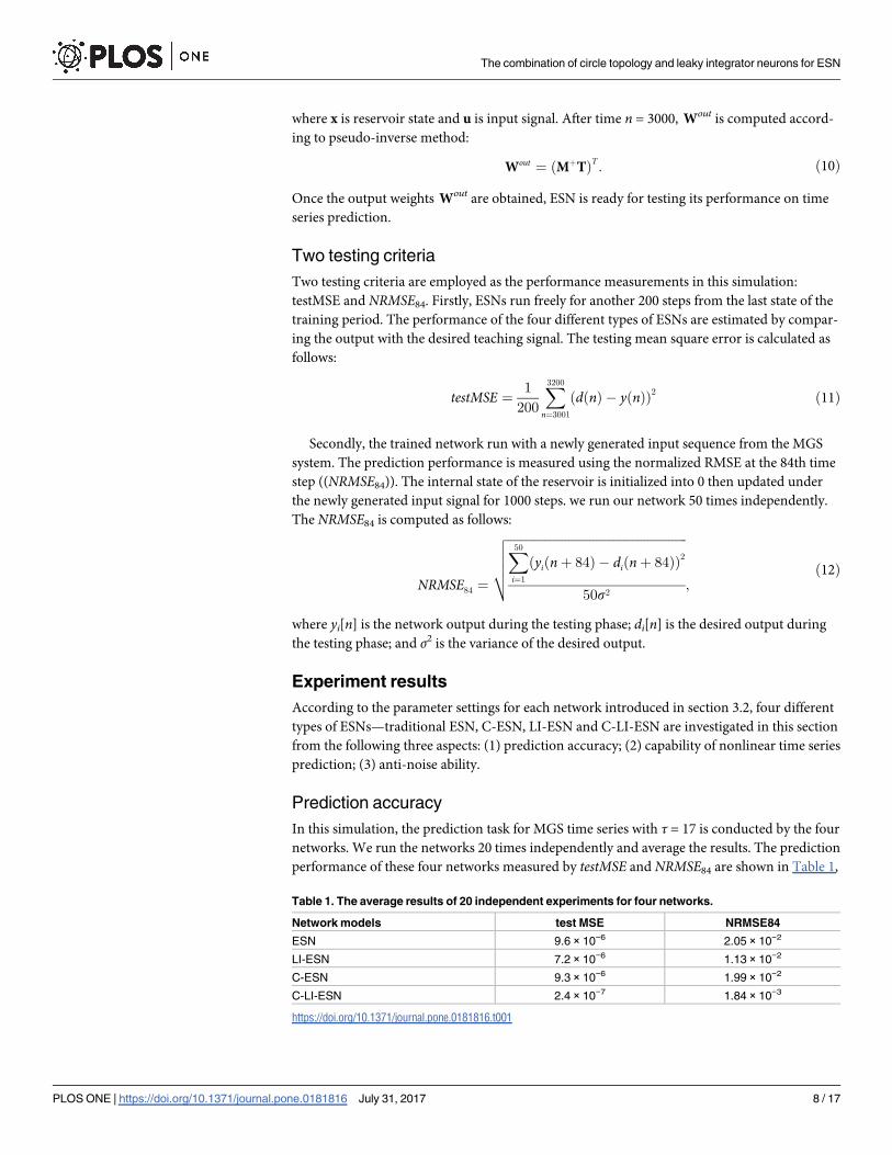
Prediction accuracy

In this simulation, the prediction task for MGS time series with τ = 17 is conducted by the four

networks. We run the networks 20 times independently and average the results. The prediction

performance of these four networks measured by testMSE and NRMSE84 are shown in Table 1,

Table 1. The average results of 20 independent experiments for four networks.

Network models test MSE NRMSE84

ESN 9.6 × 10−6 2.05 × 10−2

LI-ESN 7.2 × 10−6 1.13 × 10−2

C-ESN 9.3 × 10−6 1.99 × 10−2

C-LI-ESN 2.4 × 10−7 1.84 × 10−3

https://doi.org/10.1371/journal.pone.0181816.t001



https://doi.org/10.1371/journal.pone.0181816.t001


Figs 5 and 6. Obviously, it can be seen that the application of either cycle topology or leaky

integrator neurons alone can make ESNs achieve better performance than traditional ESN

with random reservoir and sigmoid neurons, which is consistent with the results reported in

[15, 39]. Most importantly and surprisingly, the prediction accuracy of the C-LI-ESN greatly

outperform other ESNs. The application of both cycle topology and leaky integrator neurons

make the predictive error reduced by roughly 2 orders of magnitude. The combined interac-

tions between the simple cycle topology and the leaky integrator units with memory of history

reservoir state lead to richer dynamics and lower correlation of reservoir states, which may

contribute to the remarkable enhancement of computational performance. We will discuss

these in the following paragraphs in detail.

In order to investigate the dynamical diversity of reservoir states, probability distribution of

internal reservoir states and the corresponding Wout distribution of four networks are shown

in Fig 7. It clearly shows that C-LI-ESN has much broader distribution of state values than

other networks, indicating its richest dynamic characteristics of reservoir states. Besides, the

trained Wout distribution of the C-LI-ESN is much smaller and in a more reasonable range

compared with other three networks whose output weights are in the order of 100 or even

Fig 5. The testMSEs comparisons of prediction performance for four networks.


Fig 6. The NRMSEs84 comparisons of prediction performance for four networks.







larger. Based on [40], output weights should not be too large and the reasonable absolute val-

ues are not greater than 50.

In addition a principal component analysis (PCA) of the 200 reservoir signals is conducted

as shown in Fig 8. Concretely, the reservoir state correlation matrix is estimated by R = XXT/

L, and its SVD USUT = R is computed, where the columns of U are orthonormal eigenvectors

of R (the principal component (PC) vectors), the diagonal of S contains the singular values of

R, i.e the energies (mean squared amplitudes) of the principal signal components, and L is the

sampling length during training phase. Fig 8 shows plots of these PC energies and leading PC

energies (i.e. close-up on the top ten signal energies in linear scale). The energy spectra are dif-

ferent from each other and the mean squared amplitudes of both PC energy and leading PC

energy of the C-LI-ESN are markedly greater than other three networks, which further illus-

trate the diversity of dynamic characteristic.

Moreover, the correlation of the reservoir units are investigated. The correlation coefficient

and the statistical distribution are shown in Fig 9. It shows that the correlation coefficient of

C-LI-ESN are much smaller than the others, indicating its low correlation of reservoir dynamic

of C-LI-ESN. Therefore, both the rich dynamics and low correlation of reservoir states con-

tribute to the remarkable enhancement of computational performance of C-LI-ESN.

Capability of nonlinear time series prediction

It is known that as the time delay τ gets larger the nonlinearity of MGS becomes greater as

shown in Fig 3. Fig 10 shows that the performance capability of nonlinear time series predic-

tion for all networks are gradually decreasing with time delay varying from 17 to 28 as shown

in Fig 10. However, the performance of C-LI-ESN is still obviously superior to the other three

networks. The LI-ESN performs better than ESN and C-ESN.

Fig 7. The probability distribution of all internal states and corresponding Wout distribution of four networks during training phase. (a) ESN

(b) C-ESN (c) LI-ESN (d) C-LI-ESN.






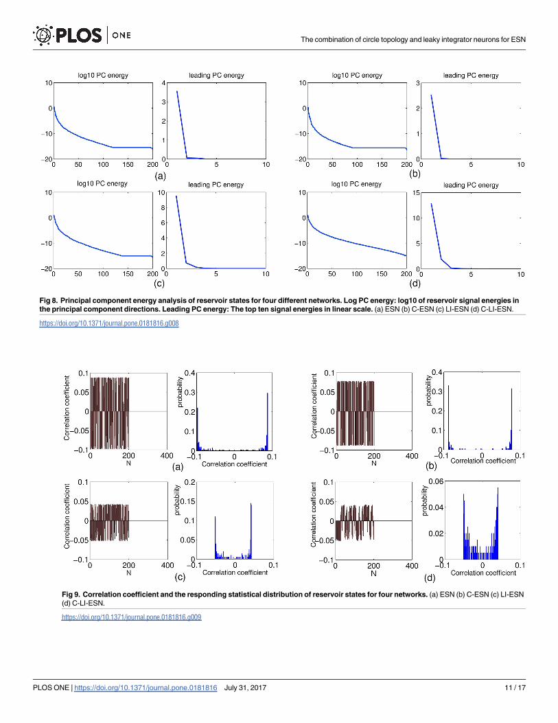
Fig 8. Principal component energy analysis of reservoir states for four different networks. Log PC energy: log10 of reservoir signal energies in

the principal component directions. Leading PC energy: The top ten signal energies in linear scale. (a) ESN (b) C-ESN (c) LI-ESN (d) C-LI-ESN.


Fig 9. Correlation coefficient and the responding statistical distribution of reservoir states for four networks. (a) ESN (b) C-ESN (c) LI-ESN

(d) C-LI-ESN.







Specifically, we set the parameter τ to be 30 and re-compare the ability of nonlinear time

series prediction for different ESN models. In this case, the Mackey-Glass system has signifi-

cantly high nonlinearity and difficult to be predicted. Our experimental results show that the

output of ESN and C-ESN become unstable as given in Fig 11(a) and 11(b). However, the out-

put of LI-ESN and C-LI-ESN can match the teacher signal well as illustrated in Fig 11(c) and

11(d). The performance of these two stable networks is further compared by calculating the

testMSE as shown in Fig 12. These results demonstrate that when the MGS becomes a high

nonlinear system, the abilities of nonlinear time series prediction for all ESNs decline. How-

ever, the C-LI-ESN and LI-ESN can show a remarkable advantage than the classical ESN.

Again, C-LI-ESN shows the best performance. Both of the memory ability of leaky integrator

units and the simple circle topology improve the ability of capturing complex characteristics of

the learning tasks.

The anti-noise ability

In [36], the authors pointed out that the pseudo-inverse training method sometimes bring up

non-stationarity phenomenon in some of the independent trials as shown in Fig 13. It can be

readily observed that the absolute value of the network output is up to 1 when the reservoir

states become unstable or divergent. It is known that injecting noise to the reservoir state during

training period can enhance the stability and robustness of trained networks. However, simulta-

neously the prediction accuracy maybe impaired with the increasing of noise intensity [1].

Fig 10. Capability of nonlinear time series prediction. The log10 testMSE of four networks vs the time delay τ in the Mackey-Glass

system.






Fig 11. Teacher signal (solid) and network output (dashed) for four networks with the parameter of learning task τ = 30.

(a) ESN (b) C-ESN (c) LI-ESN (d) C-LI-ESN.


Fig 12. Comparison of testMSEs of LI-ESN and C-LI-ESN for the learning task τ = 30. The results are

obtained by 20 independent realizations.







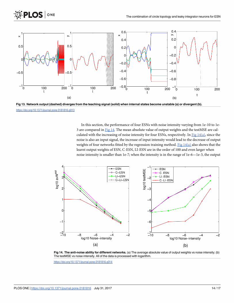
In this section, the performance of four ESNs with noise intensity varying from 1e-10 to 1e-

3 are compared in Fig 14. The mean absolute value of output weights and the testMSE are cal-

culated with the increasing of noise intensity for four ESNs, respectively. In Fig 14(a), since the

noise is also an input signal, the increase of input intensity would lead to the decrease of output

weights of four networks fitted by the regression training method. Fig 14(a) also shows that the

learnt output weights of ESN, C-ESN, LI-ESN are in the order of 100 and even larger when

noise intensity is smaller than 1e-7; when the intensity is in the range of 1e-6—1e-3, the output

Fig 13. Network output (dashed) diverges from the teaching signal (solid) when internal states become unstable (a) or divergent (b).


Fig 14. The anti-noise ability for different networks. (a) The average absolute value of output weights vs noise intensity; (b)

The testMSE vs noise intensity. All of the data is processed with logarithm.







weights of three networks achieve a reasonable range; While for C-LI-ESN, the output weight

are always kept in proper range even if the noise intensity is quite weak. From Fig 14(b), we

can observe that the C-LI-ESN can performance much better than the other three networks

during the whole range of noise intensity. The prediction accuracy of four networks all decline

with the increasing of noise intensity due to the increase of task complexity; However, since

noise is also an input signal, the increase of input intensity would lead to the decrease of output

weights fitted by the regression training method. Actually, adding noise during training is an

effective method to reduce output weights, but impair the desired accuracy as well. This result

is consistent with the observation in [1], where it also mentioned that the stability of ESNs can

be enhanced (i.e. the output weight is reduced) by adding appropriate intensity of noise, but

the computational accuracy is depressed.

Conclusion

In this paper, a new ESN model based on circle topology and leaky integrator units is pro-

posed. The effect of circle structure and leaky integrator neurons on improving the computa-

tional performance of ESN are investigated in detail. Mackey-Glass time series is used to test

the performance of four ESN networks: classical random ESN with sigmoid neurons, circle

ESN with sigmoid neurons, random ESN with leaky integrator neurons, circle ESN with leaky

integrator neurons. Comparative simulation experiments including the prediction capability,

the capability of nonlinear time series prediction, the anti-noise ability are conducted respec-

tively. The obtained experiment results show that our circle leaky integrator ESN has much

better prediction accuracy than other three ESNs due to the rich dynamical diversity and low

correlation of reservoir states. Moreover, the proposed C-LI-ESN has much stronger ability to

approximate nonlinear dynamics and resist noise than other networks, especially the conven-

tional ESN and ESN with only simple circle structure or leaky integrator neurons. The combi-

nation of circle topology and leaky integrator neurons can remarkably improve the

performance of echo state network on time series prediction. This work provides an efficient

model of ESN with excellent performance and simple network structure, which is very mean-

ingful for the broad application of ESN on various fields. There still remain open problems.

For example, strict theoretic analysis for the stability of obvious reservoir models is necessary.

Moreover, how to find the optimal values of parameters is also a difficult problem. Further

related research and extended application to other real-time or real data tasks would be our

future work.

Acknowledgments

This work is supported by the National Natural Science Foundation of China (Nos. 61473051

and 61304165), Natural Science Foundation of Chongqing (No. cstc2016jcyjA0015) and Fun-

damental Research Funds for the Central Universities (No. 106112017CDJXY170004 and Nos.

CQDXWL-2012-172). The funders had no role in study design, data collection and analysis,

decision to publish, or preparation of the manuscript.

Author Contributions

Conceptualization: Fangzheng Xue.

Formal analysis: Xiumin Li.

Funding acquisition: Fangzheng Xue.

Methodology: Fangzheng Xue.




Project administration: Fangzheng Xue.

Software: Qian Li.

Supervision: Xiumin Li.

Validation: Qian Li.

Writing – original draft: Qian Li.

Writing – review & editing: Xiumin Li.

References1. Jaeger H (2002) A tutorial on training recurrent neural networks, covering BPTT, RURL, EKF and the

echo state network approach. Technical Report GMD Report 159, German National Research Center

for Information Technology.

2. Jaeger H, Hass H (2004) Harnessing nonlinearity: predicting chaotic systems and saving energy in wire-

less telecommunication. Science(5667), pp. 78–80.

3. Li D, Han M, Wang J (2012) Chaotic time series prediction based on a novel robust echo state network.

IEEE Transactions on Neural Networks and Learning Systems, 23(5), 787–799. https://doi.org/10.

1109/TNNLS.2012.2188414 PMID: 24806127

4. Jaeger H (2003) Adaptive nonlinear system identification with echo state networks. Advances in Neural

Information Processing Systems, pp. 609–616.

5. Skowronski MD, Harris JG (2007) Noise-robust automatic speech recognition using a predictive echo

state network. IEEE Transactions on Audio Speech and Language Processing, 15(5), 1724–1730.

https://doi.org/10.1109/TASL.2007.896669

6. Skowronski MD, Harris JG (2006) Minimum mean squared error time series classification using an

echo state network prediction model. In: IEEE Int.Symp.Circuits Syst, pp. 3153–3156.

7. Wang L, Wang Z, Liu S (2016) An effective multivariate time series classification approach using echo

state network and adaptive differential evolution algorithm. Expert Systems with Applications, 43, 237–

249. https://doi.org/10.1016/j.eswa.2015.08.055

8. Peng Y, Lei M, Guo J (2011) Clustered complex echo state networks for traffic forecasting with prior

knowledge. In: Instrumentation and Measurement Technology Conference (I2MTC), pp. 1–5.

9. Bianchi FM, Scardapane S, Uncini A, Rizzi A, Sadeghian A (2015) Prediction of telephone calls load

using Echo State Network with exogenous variables. Neural Networks 71, 204–213. https://doi.org/10.

1016/j.neunet.2015.08.010 PMID: 26413714

10. Lin X, Yang Z, Song Y (2009) Short-term stock price prediction based on echo state networks. Expert

system with application, 36(3), 7313–7317. https://doi.org/10.1016/j.eswa.2008.09.049

11. Tong MH, Bicket AD, Christiansen EM, Cottrell GW (2007) Learning grammatical structure with echo

state network. Neural Networks, 20(3), 424–432. https://doi.org/10.1016/j.neunet.2007.04.013 PMID:

17556116

12. Jaeger H, Lukoeviius M, Popovici D, Siewert U (2007) Optimization and applications of echo state net-

works with leaky-integrator neurons. Neural Networks, 20(3), 335–352. https://doi.org/10.1016/j.

neunet.2007.04.016 PMID: 17517495

13. LIU X, CUI HY, ZHOU TG, CHEN JY (2012) Performance evaluation of new echo state networks based

on complex network. The Journal of China Universities of Posts and Telecommunications, 19(1), 87–

93. https://doi.org/10.1016/S1005-8885(11)60232-X

14. Deng ZD, Zhang Y (2006) Collective behavior of a small-world recurrent neural system with scale-free

distribution. IEEE Transactions on Neural Networks, 18(5), 1364–1375. https://doi.org/10.1109/TNN.

2007.894082

15. Yang B, Deng ZD (2012) An extended SHESN with leaky integrator neuron and inhibitory connection

for Mackey-Glass prediction. Frontiers of Electrical and Electronic Engineering, 7(2), 200–207.

16. Jaeger H (2007). Discovering multiscale dynamical features with hierarchical echo state networks. Vtls

Inc, 35(2), 277–284.

17. Xue Y, Yang L, Haykin S (2007) Decoupled echo state networks with lateral inhibition. Neural Networks,

20(3), 365–376. https://doi.org/10.1016/j.neunet.2007.04.014 PMID: 17517490

18. Yin J, Meng Y, Jin YC (2012) A developmental approach to structural self-organization in reservoir com-

puting. IEEE Transactions on Autonomous Mental Development, 4(4), 273–289. https://doi.org/10.

1109/TAMD.2012.2182765



https://doi.org/10.1109/TNNLS.2012.2188414

https://doi.org/10.1109/TNNLS.2012.2188414

http://www.ncbi.nlm.nih.gov/pubmed/24806127

https://doi.org/10.1109/TASL.2007.896669

https://doi.org/10.1016/j.eswa.2015.08.055

https://doi.org/10.1016/j.neunet.2015.08.010



https://doi.org/10.1016/j.eswa.2008.09.049






https://doi.org/10.1016/S1005-8885(11)60232-X

https://doi.org/10.1109/TNN.2007.894082

https://doi.org/10.1109/TNN.2007.894082



https://doi.org/10.1109/TAMD.2012.2182765

https://doi.org/10.1109/TAMD.2012.2182765


19. Chrol-Cannon J, Jin YC (2014) Computational modeling of neural plasticity for self-organization of neu-

ral networks. Biosystems, 125, 43–54. https://doi.org/10.1016/j.biosystems.2014.04.003 PMID:

24769242

20. Gao ZK, Jin ND (2012) A directed weighted complex network for characterizing chaotic dynamics from

time series. Nonlinear Analysis Real World Applications, 13(2), 947–952. https://doi.org/10.1016/j.

nonrwa.2011.08.029

21. Gao ZK, Small M, Kurths J (2016) Complex network analysis of time series. Europhysics Letters, 116

(5): 50001. https://doi.org/10.1209/0295-5075/116/50001

22. Gao ZK, Fang PC, Ding MS, et al (2015) Multivariate weighted complex network analysis for character-

izing nonlinear dynamic behavior in two-phase flow. Experimental Thermal & Fluid Science, 60, 157–

164. https://doi.org/10.1016/j.expthermflusci.2014.09.008

23. Gao ZK, Cai Q, Yang YX (2017) Visibility Graph From Adaptive Optimal-Kernel Time-Frequency Repre-

sentation for Classification of Epileptiform EEG. International Journal of Neural Systems, 27(4),

1750005. https://doi.org/10.1142/S0129065717500058 PMID: 27832712

24. Gao ZK, Yang Y, Zhai L, et al (2016) A Four-Sector Conductance Method for Measuring and Character-

izing Low Velocity Oil-Water two Phase Flows. IEEE Transactions on Instrumentation & Measurement,

65(7), 1690–1697. https://doi.org/10.1109/TIM.2016.2540862

25. Shi ZW, Han M (2007) Ridge regression learning in esn for chaotic time series prediction. Control and

Decision, 22(3), 258–257.

26. Li XM, Zhong L, Xue FZ, Zhang AG (2015) A Priori Data-driven Multi-clustered Reservoir Generation

Algorithm for Echo State Network. PLOS ONE, 10(4), e0120750. https://doi.org/10.1371/journal.pone.

0120750 PMID: 25875296

27. Shutin D, Zechner C, Kulkarni S, Poor H (2012) Regularized variational bayesian learning of echo state

networks with delay&sum readout. Neural Computation, 24(4), 967–995. https://doi.org/10.1162/

NECO_a_00253 PMID: 22168555

28. Wang S, Yang XJ, Wei CJ (2006) Harnessing Non-linearity by Sigmoid-wavelet Hybrid Echo State Net-

works (SWHESN). Proceedings of the 6th World Congress on Intelligent Control and Automation,

3014–3018. https://doi.org/10.1109/WCICA.2006.1712919

29. Holzmann G, Hauser H (2010) Echo state networks with filter neurons and a delay sum readout. Neural

Networks, 23(2), 244–256. https://doi.org/10.1016/j.neunet.2009.07.004 PMID: 19625164

30. Wang YH, Wang RB, Zhu YT (2017) Optimal path-finding through mental exploration based on neural

energy field gradients. Cognitive Neurodynamics, 11(1), 99–111. https://doi.org/10.1007/s11571-016-

9412-2 PMID: 28174616

31. Wang ZY, Wang RB, Fang RB (2015) Energy coding in neural network with inhibitory neurons. Cogni-

tive Neurodynamics, 9(2), 129–144. https://doi.org/10.1007/s11571-014-9311-3 PMID: 25806094

32. Wang ZY, Wang RB (2014) Energy distribution property and energy coding of a structural neural net-

work. Frontiers in Computational Neuroscience, 8(8), 14. https://doi.org/10.3389/fncom.2014.00014

PMID: 24600382

33. Wang RB, Zhu YT (2016) Can the activities of the large scale cortical network be expressed by neural

energy? A brief review. Cognitive Neurodynamics. 10(1), 1–5. https://doi.org/10.1007/s11571-015-

9354-0 PMID: 26834857

34. Strauss T, Wustlich W, Labahn R (2012) Design strategies for weight matrices of echo state networks.

Neural Computation, 24(12), 3246–3276. https://doi.org/10.1162/NECO_a_00374 PMID: 22970872

35. Rodan A, Tiuo P (2011) Minimum complexity echo state network. IEEE Transaction on Neural Net-

works, 22(1), 131–144. https://doi.org/10.1109/TNN.2010.2089641

36. Cui HY, Feng C, Chai Y, Liu RP, Liu YJ (2014) Effect of hybrid circle reservoir injected with wavelet-neu-

rons on performance of echo state network. Neural Networks, 57, 141–151. https://doi.org/10.1016/j.

neunet.2014.05.013 PMID: 24997457

37. Jaeger H (2001) The “echo state” approach to analyzing and training recurrent neural networks-with an

erratum note. Bonn, Germany: German ational Research Center for Information Technology GMD

Technical Report, 148, 34.

38. Lukoseviclus M, Jaeger H (2009). Reservoir computing approaches to recurrent neural network train-

ing. Computer Science Review, 3(3), 127–149. https://doi.org/10.1016/j.cosrev.2009.03.005

39. Lun SX, Yao XS, Qi HY, Hu HF (2015) A novel model of leaky integrator echo state network for time-

series prediction. Neurocomputing, 159, 58–66. https://doi.org/10.1016/j.neucom.2015.02.029

40. Jaeger H (2005) Reservoir riddles: suggestions for echo state network research. IEEE International

Joint Conference on Neural Networks. 3, 1460–1462.



https://doi.org/10.1016/j.biosystems.2014.04.003


https://doi.org/10.1016/j.nonrwa.2011.08.029

https://doi.org/10.1016/j.nonrwa.2011.08.029

https://doi.org/10.1209/0295-5075/116/50001

https://doi.org/10.1016/j.expthermflusci.2014.09.008

https://doi.org/10.1142/S0129065717500058


https://doi.org/10.1109/TIM.2016.2540862




https://doi.org/10.1162/NECO_a_00253



https://doi.org/10.1109/WCICA.2006.1712919



https://doi.org/10.1007/s11571-016-9412-2

https://doi.org/10.1007/s11571-016-9412-2


https://doi.org/10.1007/s11571-014-9311-3


https://doi.org/10.3389/fncom.2014.00014


https://doi.org/10.1007/s11571-015-9354-0

https://doi.org/10.1007/s11571-015-9354-0




https://doi.org/10.1109/TNN.2010.2089641




https://doi.org/10.1016/j.cosrev.2009.03.005

https://doi.org/10.1016/j.neucom.2015.02.029


the combination of circle topology and leaky integrator

Documents