Th

e C

oal

esce

nt

and

Mea

sura

bly

Evo

lvin

g P

op

ula

tio

ns

The Coalescent and Measurably Evolving Populations

Alexei Drummond

Department of Computer Science

University of Auckland, NZ

Th

e C

oal

esce

nt

and

Mea

sura

bly

Evo

lvin

g P

op

ula

tio

ns Overview

1. Introduction to the Coalescent

2. Hepatitis C in Egypt• An example using the coalescent

3. Measurably evolving populations

4. HIV-1 evolution within and among hosts• An example using MEP concepts

5. Summary + Conclusions

Th

e C

oal

esce

nt

and

Mea

sura

bly

Evo

lvin

g P

op

ula

tio

ns The coalescent

• The coalescent is a model of the ancestral relationships of a small sample of individuals taken from a large background population.

• The coalescent describes a probability distribution on ancestral genealogies (trees) given a population history. – Therefore the coalescent can convert information from ancestral

genealogies into information about population history and vice versa.

• The coalescent is a model of ancestral genealogies, not sequences, and its simplest form assumes neutral evolution.

Th

e C

oal

esce

nt

and

Mea

sura

bly

Evo

lvin

g P

op

ula

tio

ns The history of coalescent theory

• 1930-40s: Genealogical arguments well known to Wright & Fisher

• 1964: Crow & Kimura: Infinite Allele Model

• 1966: (Hubby & Lewontin) & (Harris) make first surveys of population allele variation by protein electrophoresis

• 1968: Motoo Kimura proposes neutral explanation of molecular evolution & population variation. So do King & Jukes

• 1971: Kimura & Ohta proposes infinite sites model.

• 1975: Watterson makes explicit use of “The Coalescent”

• 1982: Kingman introduces “The Coalescent”.

• 1983: Hudson introduces “The Coalescent with Recombination”

• 1983: Kreitman publishes first major population sequences.

• 1987: Cann et al. traces human origin and migrations with mitochondrial DNA.

Th

e C

oal

esce

nt

and

Mea

sura

bly

Evo

lvin

g P

op

ula

tio

ns The history of coalescent theory

• 1988: Hughes & Nei: Genes with positive Darwinian Selection.

• 1989-90: Kaplan, Hudson, Takahata and others: Selection regimes with coalescent structure (MHC, Incompatibility alleles).

• 1991: MacDonald & Kreitman: Data with surplus of replacement interspecific substitutions.

• 1994-95: Griffiths-Tavaré + Kuhner-Yamoto-Felsenstein introduces sampling techniques to estimate parameters in population models.

• 1997-98: Krone-Neuhauser introduces Ancestral Selection Graph

• 1999: Wiuf & Donnelly uses coalescent theory to estimate age of disease allele

• 2000: Wiuf et al. introduces gene conversion into coalescent.

• 2000-: A flood of SNP data & haplotypes are on their way.

Th

e C

oal

esce

nt

and

Mea

sura

bly

Evo

lvin

g P

op

ula

tio

ns Population processes

Genealogy

COALESCENT

THEORY

Th

e C

oal

esce

nt

and

Mea

sura

bly

Evo

lvin

g P

op

ula

tio

ns

Randomly sample individuals from population

Obtain gene sequences from sampled individuals

Reconstruct tree / trees from sequences

Infer coalescent results from tree / trees

Infer coalescent results directly from sequences

Coalescent inference

Th

e C

oal

esce

nt

and

Mea

sura

bly

Evo

lvin

g P

op

ula

tio

ns Demographic History

• Change in population size through time

• Applications include– Estimating history of human populations– Conservation biology– Reconstructing infectious disease epidemics– Investigating viral dynamics within hosts

Th

e C

oal

esce

nt

and

Mea

sura

bly

Evo

lvin

g P

op

ula

tio

ns Idealized Wright-Fisher populations

Now

Parents

Grand parents

Haploid Diploid

Th

e C

oal

esce

nt

and

Mea

sura

bly

Evo

lvin

g P

op

ula

tio

ns Random mating in an ideal population

•A constant population size of N individuals•Each individual in the new generation “chooses” its parent from the previous generation at random

Th

e C

oal

esce

nt

and

Mea

sura

bly

Evo

lvin

g P

op

ula

tio

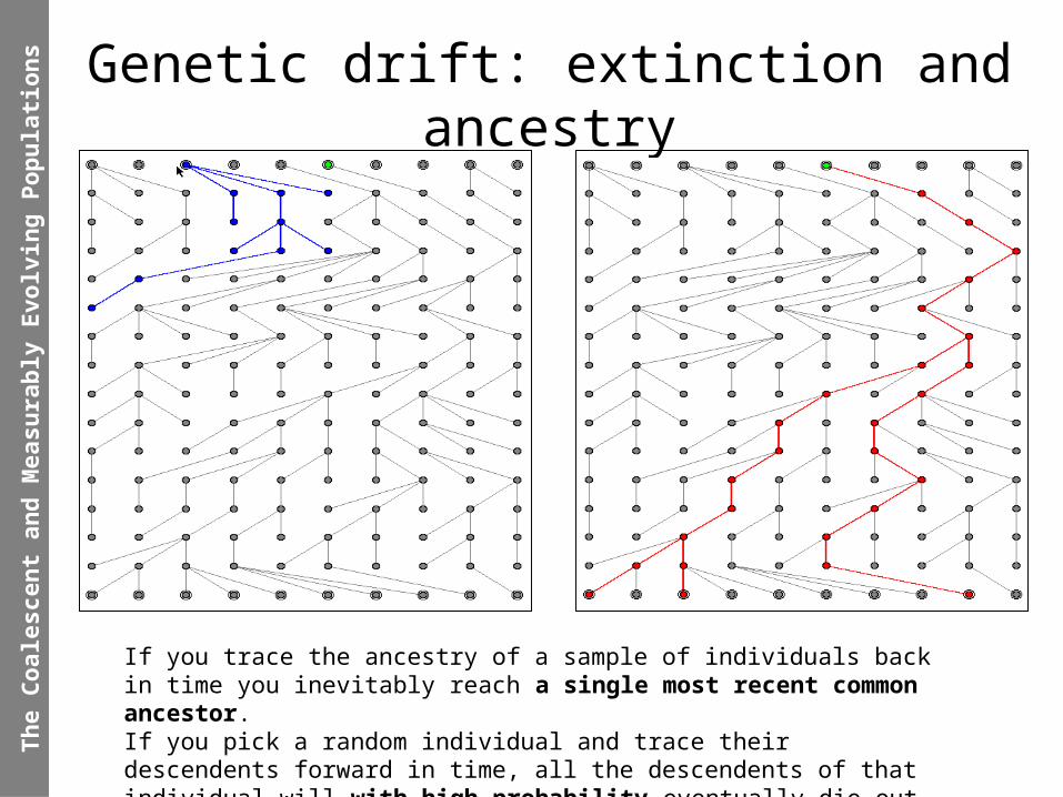
ns Genetic drift: extinction and ancestry

If you trace the ancestry of a sample of individuals back in time you inevitably reach a single most recent common ancestor.If you pick a random individual and trace their descendents forward in time, all the descendents of that individual will with high probability eventually die out.

Th

e C

oal

esce

nt

and

Mea

sura

bly

Evo

lvin

g P

op

ula

tio

ns

Dis

cret

e G

ener

atio

ns

Present

PastA sample genealogy of 3 sequences from a population (N =10).

Present

Past

A sample genealogy from an idealized Wright-Fisher population

Th

e C

oal

esce

nt

and

Mea

sura

bly

Evo

lvin

g P

op

ula

tio

ns

The coalescent: distributions and expectations on a sample genealogy

Present

Past

t2 ~ Exp(N)

t3 ~ Exp N /3

E[t3]N /3

E[t2]N

E[tk ]2N

k(k 1)

E[troot ]2N 11

n

Th

e C

oal

esce

nt

and

Mea

sura

bly

Evo

lvin

g P

op

ula

tio

ns

The coalescent: probability density distribution

Present

Past

P(t2 | N) 1

Nexp

t2

N

P(t3 | N) 3

Nexp

3t3

N

fG (g | N) k(k 1)

Nexp

k(k 1)tk

N

k2

n

dg

t2 ~ Exp(N)

t3 ~ Exp N /3

Kingman (1982a,b)

g Eg ,t The genealogy is an edge graph Eg and a vector of times t.

Th

e C

oal

esce

nt

and

Mea

sura

bly

Evo

lvin

g P

op

ula

tio

ns

The coalescent: estimating population size from a sample genealogy

Present

Past

ˆ N k k(k 1)

2tk

ˆ N 3 24

ˆ N 2 7

ˆ N 1

n 1

k(k 1)

2tk

k2

n

ˆ N 15.5

t2 7

t3 8

Felsenstein (1992)

Th

e C

oal

esce

nt

and

Mea

sura

bly

Evo

lvin

g P

op

ula

tio

ns

The coalescent: estimating population size confidence limits via ML

Maximum likelihood can be used to estimate population size by choosing a population size that maximizes the probability of the observed coalescent waiting times.

The confidence intervals are calculated from the curvature of the likelihood. For a single parameter model the 95% confidence limits are defined by the points where the log-likelihood drops 1.92 log-units below the maximum log-likelihood.

-20

-18

-16

-14

-12

-10

-8

-6

1 10 100 1000

Population size (N)

rela

tive log lik

elihood

ˆ N 15.5 (5.1, 93.1)

Th

e C

oal

esce

nt

and

Mea

sura

bly

Evo

lvin

g P

op

ula

tio

ns

Exponential growth Constant size

The coalescent: shapes of gene genealogies

The coalescent can be used to convert coalescent times into knowledge about population size and its change though time.

Th

e C

oal

esce

nt

Th

e C

oal

esce

nt

and

Mea

sura

bly

Evo

lvin

g P

op

ula

tio

ns

smallsmall NN00 large large NN00

TIMETIME

Constant population size: N(t)=N0

Th

e C

oal

esce

nt

Th

e C

oal

esce

nt

and

Mea

sura

bly

Evo

lvin

g P

op

ula

tio

ns Coalescent and serial samples

Constant population Exponential growth

Th

e C

oal

esce

nt

Th

e C

oal

esce

nt

and

Mea

sura

bly

Evo

lvin

g P

op

ula

tio

ns Uncertainty in Genealogies

Th

e C

oal

esce

nt

How similar are these two trees? Both of them are plausible given the data.

We can use MCMC to get the average result over all plausible trees,

Th

e C

oal

esce

nt

and

Mea

sura

bly

Evo

lvin

g P

op

ula

tio

ns Coalescent Summary

• The coalescent provides a theory of how population size is related to the distribution of coalescent events in a tree.

• Big populations have old trees• Exponentially growing populations have star-like trees• Given a genealogy the most likely population size can be

estimated.• MCMC can be used to get a distribution of trees from

which a distribution of population sizes can be estimated.

Th

e C

oal

esce

nt

Th

e C

oal

esce

nt

and

Mea

sura

bly

Evo

lvin

g P

op

ula

tio

ns Markov chain Monte Carlo (MCMC)

MC

MC

• Imagine you would like to estimate two parameters (,) from some data (D).

• You want to find values of and that have high probability given the data: p(,|D)

• Say you have a likelihood function of the form: Pr{D| ,}

• Bayes rule tells us that:– p(,|D) = Pr{D| ,}p(,) / Pr{D}– So that p(,|D) Pr{D| ,}p(,)

Th

e C

oal

esce

nt

and

Mea

sura

bly

Evo

lvin

g P

op

ula

tio

ns Markov chain Monte Carlo (MCMC)

MC

MC

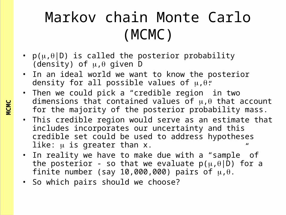
• p(,|D) is called the posterior probability (density) of , given D• In an ideal world we want to know the posterior density for all

possible values of ,.• Then we could pick a “credible region” in two dimensions that

contained values of , that account for the majority of the posterior probability mass.

• This credible region would serve as an estimate that includes incorporates our uncertainty and this credible set could be used to address hypotheses like: is greater than x.

• In reality we have to make due with a “sample” of the posterior - so that we evaluate p(,|D) for a finite number (say 10,000,000) pairs of ,.

• So which pairs should we choose?

Th

e C

oal

esce

nt

and

Mea

sura

bly

Evo

lvin

g P

op

ula

tio

ns Markov chain Monte Carlo (MCMC)

MC

MC

• Lets construct a random walk in 2-dimensional space• In each step of the random walk we propose to make an (unbiased)

small jump from our current position (,) to a new position (’,’) • If p(’,’|D) > p(,|D) then we make the proposed jump• However, if p(’,’|D) < p(,|D), then we make the proposed jump

with probability = p(’,’|D) / p(,|D), otherwise we stay where we are.

• It can be shown (trust me!) that if you proceed in this fashion for an infinite time then the equilibrium distribution of this random walk will be p(,|D)!

• That is, the random walk will visit a particular region [0, 1] x [0, 1] of the state space this often:

p(, | D)dd 0

1

0

1

Th

e C

oal

esce

nt

and

Mea

sura

bly

Evo

lvin

g P

op

ula

tio

ns Markov chain Monte Carlo (MCMC)

MC

MC

p(, | D) Z Pr{D |,g} f ( | g) f (,)g

Th

e C

oal

esce

nt

and

Mea

sura

bly

Evo

lvin

g P

op

ula

tio

ns Hepatitis C Virus (HCV)

Po

pu

lati

on

gen

etic

s o

f H

epat

itis

C in

Eg

ypt

• Identified in 1989• 9.6kb single-stranded RNA genome • Polyprotein cleaved by proteases• No efficient tissue culture system

Th

e C

oal

esce

nt

and

Mea

sura

bly

Evo

lvin

g P

op

ula

tio

ns How important is HCV?

• 170m+ infected• ~80% infections are chronic• Liver cirrhosis & cancer risk• 10,000 deaths per year in

USA• No protective immunity?

Po

pu

lati

on

gen

etic

s o

f H

epat

itis

C in

Eg

ypt

Th

e C

oal

esce

nt

and

Mea

sura

bly

Evo

lvin

g P

op

ula

tio

ns

Percutaneous exposure to infected bloodPercutaneous exposure to infected blood

• Blood transfusion / blood products

• Injecting & nasal drug use

• Sexual & vertical transmission

• Unsafe injections

• Unidentified routes

HCV Transmission

Po

pu

lati

on

gen

etic

s o

f H

epat

itis

C in

Eg

ypt

Th

e C

oal

esce

nt

and

Mea

sura

bly

Evo

lvin

g P

op

ula

tio

ns

Estimating demographic history of HCV using the coalescent

• Egyptian HCV gene sequences

• n=61

• E1 gene, 411bp

• All sequence contemporaneous

• Egypt has highest prevalence of HCV worldwide (10-20%)

• But low prevalence in neighbouring states

• Why is Egypt so seriously affected?

• Parenteral antischistosomal therapy (PAT)

Po

pu

lati

on

gen

etic

s o

f H

epat

itis

C in

Eg

ypt

Th

e C

oal

esce

nt

and

Mea

sura

bly

Evo

lvin

g P

op

ula

tio

ns Demographic model

• The coalescent can be extended to model deterministically varying populations.

• The model we used was a const-exp-const model.

• A Bayesian MCMC method was developed to sample the gene genealogy, the substitution model and demographic function simultaneously.

N(t)NC if t x

NC exp[ r(t x)] if x t y

NA if t y

Po

pu

lati

on

gen

etic

s o

f H

epat

itis

C in

Eg

ypt

Th

e C

oal

esce

nt

and

Mea

sura

bly

Evo

lvin

g P

op

ula

tio

ns Estimated demographic history

Po

pu

lati

on

gen

etic

s o

f H

epat

itis

C in

Eg

ypt

Averaged over all trees

Based on a single tree

Th

e C

oal

esce

nt

and

Mea

sura

bly

Evo

lvin

g P

op

ula

tio

ns Parameter estimates

Po

pu

lati

on

gen

etic

s o

f H

epat

itis

C in

Eg

ypt

Th

e C

oal

esce

nt

and

Mea

sura

bly

Evo

lvin

g P

op

ula

tio

ns Uncertainty in parameter estimates

Growth rate of the growth phase

Grey box is the prior

Rates at different codon positions,

All significantly different

Demographic parameters Mutational parameters

Po

pu

lati

on

gen

etic

s o

f H

epat

itis

C in

Eg

ypt

Th

e C

oal

esce

nt

and

Mea

sura

bly

Evo

lvin

g P

op

ula

tio

ns Full Bayesian Estimation

• Marginalized over uncertainty in genealogy and mutational processes

• Yellow band represents the region over which PAT was employed in Egypt

Po

pu

lati

on

gen

etic

s o

f H

epat

itis

C in

Eg

ypt

Th

e C

oal

esce

nt

and

Mea

sura

bly

Evo

lvin

g P

op

ula

tio

ns

Measurably evolving populations (MEPs)

Present time point (n = 5)

Earlier time point (n = 5)

• MEP pathogens:– HIV – Hepatitis C– Influenza A

• MEPs from ancient DNA– Bison– Brown Bears– Adelie penguins– Anything cold and numerous

• Even over short periods (less than a year) HIV sequences can exhibit measurable evolutionary change

• Time-structure can not be ignored in our models

Mea

sura

bly

evo

lvin

g p

op

ula

tio

ns

Th

e C

oal

esce

nt

and

Mea

sura

bly

Evo

lvin

g P

op

ula

tio

ns Time structure in samples

timeContemporary sampleno time structure

Serial samplewith time structure

2000

1980

1990

Mea

sura

bly

evo

lvin

g p

op

ula

tio

ns

Th

e C

oal

esce

nt

and

Mea

sura

bly

Evo

lvin

g P

op

ula

tio

ns

Ne

time

AB

CD

E

Molecular evolution and population genetics of MEPs

• Given sequence data that is time-structured estimate true values of:– substitution parameters

• Overall substitution rate and relative rates of different substitutions

– population history: N(t)– Ancestral genealogy

• Topology• Coalescent times

Mea

sura

bly

evo

lvin

g p

op

ula

tio

ns

Th

e C

oal

esce

nt

and

Mea

sura

bly

Evo

lvin

g P

op

ula

tio

ns

Molecular evolutionary model: Felsenstein’s likelihood (1981)

b1

b2 b5

b4

b3

AAAC

GA

GCThe probability of the sequence alignment,

can be efficiently calculated given a tree and branch lengths (T), and a probabilistic model of mutation represented by an instantaneous rate matrix (Q). In phylogenetics, branch lengths are usually unconstrained.

Pr{D | T,Q}

Th

e C

oal

esce

nt

and

Mea

sura

bly

Evo

lvin

g P

op

ula

tio

ns

Combining the coalescent with Felsenstein’s likelihood

b1

b2 b5

b4

b3

AA

AC

GA

GC

t2

t4

t3

AA

GA AC GC

The “molecular clock” constraint

2n–3 branch lengths n–1 waiting times

p(N,g,Q | D)Pr{D |g,Q} fG (g | N) fN (N) fQ (Q)

The joint posterior probability of the population history (N), the genealogy (g) and the mutation matrix (Q) are estimated using Markov chain Monte Carlo (Drummond et al, Genetics, 2002)

Th

e C

oal

esce

nt

and

Mea

sura

bly

Evo

lvin

g P

op

ula

tio

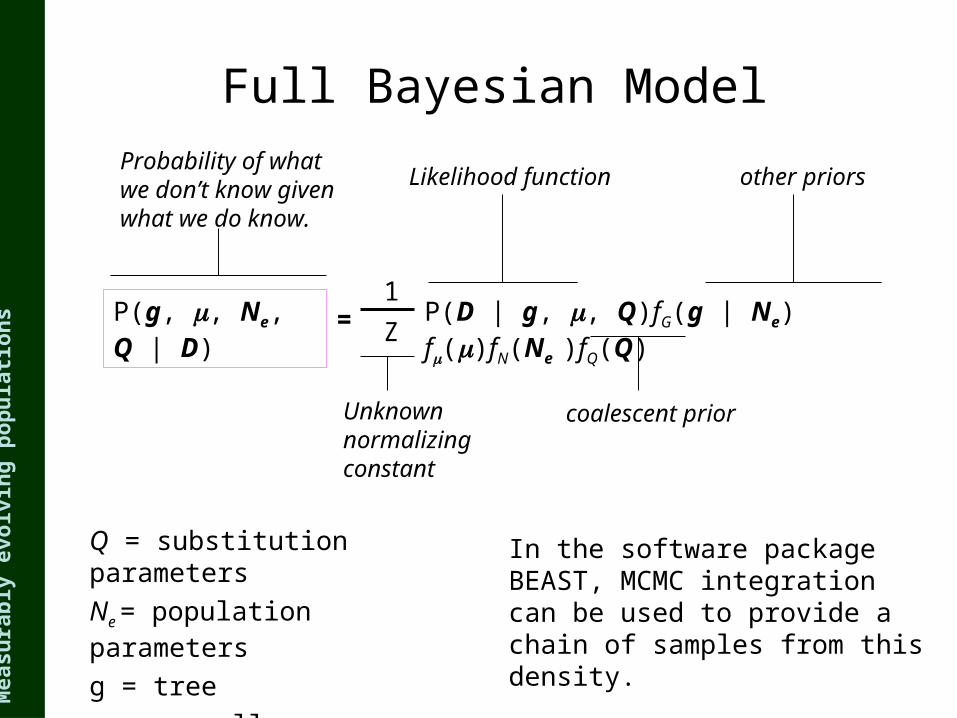
ns Full Bayesian Model

P(g, , Ne, Q | D) Z

1P(D | g, , Q)fG(g | Ne) f()fN(Ne )fQ(Q)

Probability of what we don’t know given what we do know.

Unknown normalizing constant

Likelihood function

coalescent prior

other priors

=

In the software package BEAST, MCMC integration can be used to provide a chain of samples from this density.

Mea

sura

bly

evo

lvin

g p

op

ula

tio

ns

Q = substitution parameters

Ne = population parameters

g = tree

= overall substitution rate

Th

e C

oal

esce

nt

and

Mea

sura

bly

Evo

lvin

g P

op

ula

tio

ns

Pt.7

Pt.9

HIV1U36148

HIV1U36015HIV1U35980

HIV1U36073

HIV1U35926

HIVU95460

Pt.2

Patient #6 fromWolinsky et al.

Pt.5

Pt.3Pt.1Pt.8

Pt.6

10%

Shankarappa et al (1999)

HIV-1 (env) evolution in nine infected individuals

Mea

sura

bly

evo

lvin

g p

op

ula

tio

ns

Th

e C

oal

esce

nt

and

Mea

sura

bly

Evo

lvin

g P

op

ula

tio

ns

Molecular clock: HIV-1 (env) evolution in 9 individuals

0 2 4 6 8 10

Years Post Seroconversion

Viral Divergence

2%

4%

6%

8%

10%

Shankarappa et al (1999)

Mea

sura

bly

evo

lvin

g p

op

ula

tio

ns

Th

e C

oal

esce

nt

and

Mea

sura

bly

Evo

lvin

g P

op

ula

tio

ns MEP Summary

• Most RNA viruses, including HCV and HIV are measurably evolving

• Most vertebrate populations that have well-preserved recent fossil records are MEPs.

• If sequence data comes from different times the time-structure can’t be ignored

• Time structure permits the direct estimation of:– substitution rate– Concerted changes in substitution rate– coalescent times in calendar units– Demographic function N(t) in calendar units

Mea

sura

bly

evo

lvin

g p

op

ula

tio

ns

Th

e C

oal

esce

nt

and

Mea

sura

bly

Evo

lvin

g P

op

ula

tio

ns

Intermission

My brain is fried!

Th

e C

oal

esce

nt

and

Mea

sura

bly

Evo

lvin

g P

op

ula

tio

ns

• HIV is a retrovirus.

• Within infected individuals HIV exhibits extremely high genetic variability due to:

– Error-prone reverse transcriptase (RT) that converts RNA to DNA (error rate is about one mutation per genome per replication cycle).

– DNA-dependent polymerase also error-prone

– High turnover of virus within infected individual throughout infection.

HIV virion

HIV gp120 binds to CD4 T cell surface receptors

viral core inserted into cell

replication of virus genome by reverse transcription (ssRNA to dsDNA)

integration of proviral DNA into DNA of infected cell

viral RNA transcription

regulatory genes

migration of dsDNA to nucleus

viral genomic RNA

RNA packaging and virion assembly

structural proteins and viral enzymes

translation

LTRLTR

budding of virus from cell and maturation

nucleus

host cell

What is HIV?

Po

pu

lati

on

gen

etic

s o

f H

IV

Th

e C

oal

esce

nt

and

Mea

sura

bly

Evo

lvin

g P

op

ula

tio

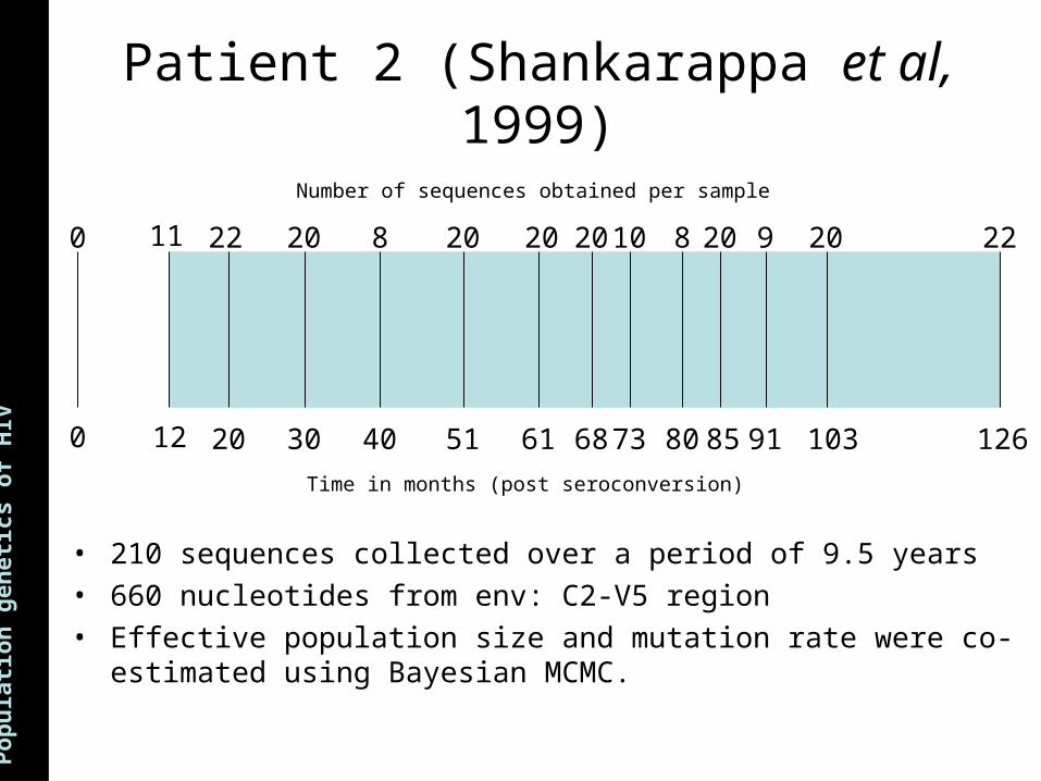
ns Patient 2 (Shankarappa et al, 1999)

0

0

12 20 30 40 51 61 68 73 80 85 91 103 126

11 22 20 8 20 20 20 10 8 20 9 20 22

Time in months (post seroconversion)

Number of sequences obtained per sample

• 210 sequences collected over a period of 9.5 years• 660 nucleotides from env: C2-V5 region• Effective population size and mutation rate were co-estimated using

Bayesian MCMC.Po

pu

lati

on

gen

etic

s o

f H

IV

Th

e C

oal

esce

nt

and

Mea

sura

bly

Evo

lvin

g P

op

ula

tio

ns

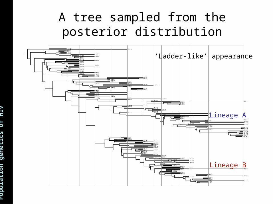
A tree sampled from the posterior distribution

Lineage A

Lineage B

‘Ladder-like’ appearance

Po

pu

lati

on

gen

etic

s o

f H

IV

Th

e C

oal

esce

nt

and

Mea

sura

bly

Evo

lvin

g P

op

ula

tio

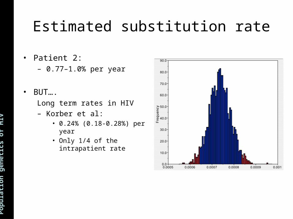
ns Estimated substitution rate

• Patient 2:– 0.77–1.0% per year

• BUT….Long term rates in HIV

– Korber et al:• 0.24% (0.18-0.28%) per year• Only 1/4 of the intrapatient

rate

Po

pu

lati

on

gen

etic

s o

f H

IV

Th

e C

oal

esce

nt

and

Mea

sura

bly

Evo

lvin

g P

op

ula

tio

ns Bayesian MCMC of Shankarappa data

estimate upper limitp1 Logistic 0.0123 882 0.278 1.57% 6.68%p2 plasma Logistic 0.0166 1708 0.242 0.63% 3.34%p2 provirus Logistic 0.0090 2798 0.278 0.04% 0.18%p3 Logistic 0.0175 620 0.237 1.80% 4.97%p5 plasma Exponential 0.0223 938 0.192 11.80% 27.50%p5 provirus Logistic 0.0215 1345 0.293 8.19% 15.20%p6 Logistic 0.0195 581 0.221 0.52% 1.35%p7 Logistic 0.0085 3320 0.322 2.94% 13.60%p8 Exponential 0.0162 2309 0.455 28.70% 48.50%p9 Logistic 0.0071 2757 0.346 17.90% 44.80%p11 Logistic 0.0128 2502 0.239 0.15% 0.53%

Overall Logistic 0.0148 1796 0.282 6.75% 15.15%* At the time of last sample assuming a generation length of 2.6 days

Bottleneck (at seroconversion)

Patient

Best-fitting demographic

modelEstimated rate

(per site per year)

Effective population

size*

Rate heterogeneity

(alpha parameter)

Mea

sura

bly

evo

lvin

g p

op

ula

tio

ns

Th

e C

oal

esce

nt

and

Mea

sura

bly

Evo

lvin

g P

op

ula

tio

ns

Intra- and inter- patient rate estimates (C2V3 envelope)

0.00E+00

5.00E-03

1.00E-02

1.50E-02

2.00E-02

2.50E-02

3.00E-02

0 50 100 150 200 250

Sampling interval (months)

rate

(p

er

sit

e p

er

year)

Intrapatient estimates

Interpatient estimates

BAC

p1 - p11

Po

pu

lati

on

gen

etic

s o

f H

IV

Th

e C

oal

esce

nt

and

Mea

sura

bly

Evo

lvin

g P

op

ula

tio

ns Summary: HIV intra-patient evolution

• HIV evolutionary rates appear to be faster intra-patient then across pandemic– Different selection pressure at transmission?– Transmitted viruses undergoing less rounds of

replication?– Latent viruses?– Reversion of escape mutants?

• Effective population size is changing over time (bottleneck in envelope at least)

Po

pu

lati

on

gen

etic

s o

f H

IV

Th

e C

oal

esce

nt

and

Mea

sura

bly

Evo

lvin

g P

op

ula

tio

ns But how good is our best model?

• We can use standard statistical model-choice criteria to choose between different models of substitution and demography, but are any of the models we consider any good at all?

• One way to look at this is ask the following question:– Does our real data look anything like what we would

expect data from our model to look like?

• So what aspect of the data should we look at?

• And what should we expect?

Go

od

nes

s-o

f-fi

t te

sts

Th

e C

oal

esce

nt

and

Mea

sura

bly

Evo

lvin

g P

op

ula

tio

ns

We could look at branch length distributions…

E[Ln ]2Ne

E[Jn ]2Ne

1

kk1

n 1

E[troot ]2Ne 11

n

troot

Ln

Jn Ln

Go

od

nes

s-o

f-fi

t te

sts

Th

e C

oal

esce

nt

and

Mea

sura

bly

Evo

lvin

g P

op

ula

tio

ns

Tree imbalance measures might also be interesting…

4 cherries 3 cherries 2 cherries

Ic 0

Ic 0.24

Ic 0.81

N 3

N 3.125

N 4.125

Go

od

nes

s-o

f-fi

t te

sts

Th

e C

oal

esce

nt

and

Mea

sura

bly

Evo

lvin

g P

op

ula

tio

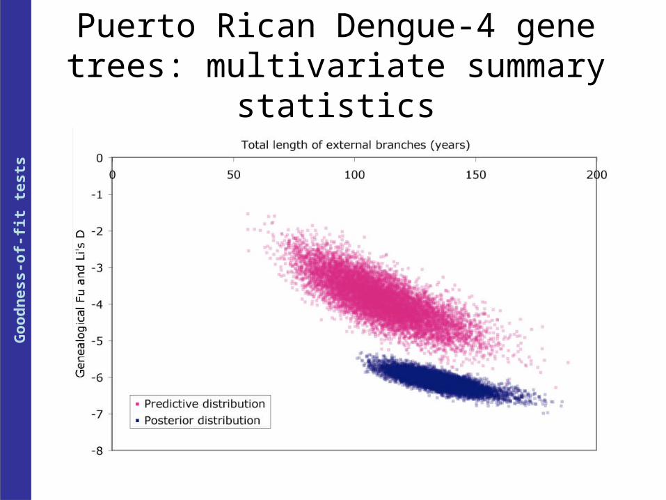
ns Posterior predictive simulation

• A method of testing the goodness-of-fit of a Bayesian model.

1. Run a Bayesian MCMC analysis on the data2. Calculate the value of your favourite summary statistic, T(.)

from the data, D3. For each state in the chain

1. Simulate a synthetic dataset, Di, using the parameter values of state i.

2. Calculate T(Di) from the simulated data set.

4. Compare the T(D) value with predictive distribution of T(Di)

Po

ster

ior

pre

dic

tive

sim

ula

tio

n

Th

e C

oal

esce

nt

and

Mea

sura

bly

Evo

lvin

g P

op

ula

tio

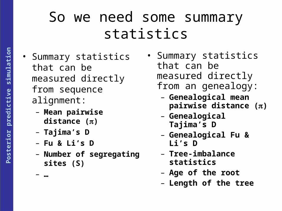
ns So we need some summary statistics

• Summary statistics that can be measured directly from sequence alignment:– Mean pairwise distance

()– Tajima’s D– Fu & Li’s D– Number of segregating

sites (S)– …

• Summary statistics that can be measured directly from an genealogy:– Genealogical mean

pairwise distance ()– Genealogical Tajima’s D– Genealogical Fu & Li’s D– Tree-imbalance statistics– Age of the root– Length of the treeP

ost

erio

r p

red

icti

ve s

imu

lati

on

Th

e C

oal

esce

nt

and

Mea

sura

bly

Evo

lvin

g P

op

ula

tio

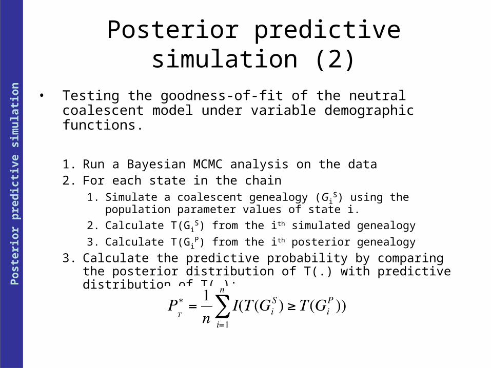
ns Posterior predictive simulation (2)

• Testing the goodness-of-fit of the neutral coalescent model under variable demographic functions.

1. Run a Bayesian MCMC analysis on the data2. For each state in the chain

1. Simulate a coalescent genealogy (GiS) using the population parameter

values of state i.

2. Calculate T(GiS) from the ith simulated genealogy

3. Calculate T(GiP) from the ith posterior genealogy

3. Calculate the predictive probability by comparing the posterior distribution of T(.) with predictive distribution of T(.):

Po

ster

ior

pre

dic

tive

sim

ula

tio

n

Th

e C

oal

esce

nt

and

Mea

sura

bly

Evo

lvin

g P

op

ula

tio

ns Human influenza A (HA gene) trees

Posterior genealogy Predictive simulations

State 5m

State 10m

Ne 9.12

t2 11.03 years

Ne 5.00

t2 15.29 years

Go

od

nes

s-o

f-fi

t te

sts

Th

e C

oal

esce

nt

and

Mea

sura

bly

Evo

lvin

g P

op

ula

tio

ns

Human influenza A trees: Genealogical Fu & Li’s D statistic

Go

od

nes

s-o

f-fi

t te

sts

Th

e C

oal

esce

nt

and

Mea

sura

bly

Evo

lvin

g P

op

ula

tio

ns

Puerto Rican Dengue-4 gene trees: multivariate summary statistics

Go

od

nes

s-o

f-fi

t te

sts

Th

e C

oal

esce

nt

and

Mea

sura

bly

Evo

lvin

g P

op

ula

tio

ns Results of test of neutrality

Table 2. The predictive probabilities (

PT) for summary statistics on each of the example

data sets are shown. Significant departures from neutrality are marked (*) and marginallysignificant departures (x < 0.05 or x > 0.95) are marked with (†). Significant departureson the best fitting model for each data set are in bold.

Predictive probabilitiesDataset Demographic

modelT troot DFL IC Cn B1

Brown bear Constant 0.739 0.815 0.863 0.693 0.163 0.103

(d-loop) Exponential growth 0.615 0.623 0.800 0.679 0.163 0.111

RSVA Constant 0.956† 0.964† 0.946 0.163 0.152 0.134

(g gene) Exponential growth 0.693 0.656 0.884 0.206 0.149 0.134

Dengue-4 Constant 0.9574† 0.9958* 0.9997* 0.562 0.608 0.427

(E gene) Exponential growth 0.745 0.809 0.9792* 0.559 0.653 0.505

Human influenza A Constant 0.9510† 0.900 0.9999* 0.0462† 0.605 0.610

(HA) Exponential growth 0.910 0.620 0.9995* 0.0866 0.575 0.677

Go

od

nes

s-o

f-fi

t te

sts

Th

e C

oal

esce

nt

and

Mea

sura

bly

Evo

lvin

g P

op

ula

tio

ns

Results for 28 HIV-1 infected individuals

Go

od

nes

s-o

f-fi

t te

sts

Fu & Li's D

0.0

0.1

0.2

0.3

0.4

0.5

0.6

0.7

0.8

0.9

1.0

0.0 0.2 0.4 0.6 0.8 1.0

proportion of data sets

P*

Sim Constant sizeSim Exponential GrowthTargetConstant sizeExponential Growth

Th

e C

oal

esce

nt

and

Mea

sura

bly

Evo

lvin

g P

op

ula

tio

ns Is the population size constant?

Patient 2

Po

pu

lati

on

gen

etic

s o

f H

IV

Pop size

10

100

1000

0 20 40 60 80 100 120

months (post seroconversion)

Ne /

30

mean

lower

upper

Th

e C

oal

esce

nt

and

Mea

sura

bly

Evo

lvin

g P

op

ula

tio

ns

Virus population dynamics

Measles virus

Human influenza virus

Ph

ylo

dyn

amic

s

Th

e C

oal

esce

nt

and

Mea

sura

bly

Evo

lvin

g P

op

ula

tio

ns

Dengue-4: Modeling complex demography

Hospital case data courtesy of Shannon Bennett

N(t) = N0exp(-rt): -10566.421N(t) = scaled translated case data: -10478.572

Ph

ylo

dyn

amic

s

Th

e C

oal

esce

nt

and

Mea

sura

bly

Evo

lvin

g P

op

ula

tio

ns Population size changes

Po

pu

lati

on

siz

e ch

ang

es

Th

e C

oal

esce

nt

and

Mea

sura

bly

Evo

lvin

g P

op

ula

tio

ns The generalized skyline plot

• Visual framework for exploring the demographic history of sampled DNA sequences

• Input: a single estimated ancestral genealogy (a tree)• Output: nonparametric plot of the population size through time

– Groups adjacent coalescent intervals

– Converts information within these intervals to estimates of population size

Po

pu

lati

on

siz

e ch

ang

es

ˆ N k k(k 1)

2tk

ˆ N k,l k(k l)

2lti

ik l1

k

Estimate of population size from single coalescent interval

Estimate of population size from l adjacent coalescent intervals.

Th

e C

oal

esce

nt

and

Mea

sura

bly

Evo

lvin

g P

op

ula

tio

ns Examples

I: Constant population size

N(t)=N(0)

Gen

eral

ized

Sky

line

Plo

t

Th

e C

oal

esce

nt

and

Mea

sura

bly

Evo

lvin

g P

op

ula

tio

ns Skyline Plot

I: Constant population size

N(t)=N(0)

II: Exponential growth

N(t)=N(0)e-rt

Gen

eral

ized

Sky

line

Plo

t

Th

e C

oal

esce

nt

and

Mea

sura

bly

Evo

lvin

g P

op

ula

tio

ns Skyline Plot

III: HIV-1 group M(tree estimated in Yusim et al (2001) Phil. Trans. Roy. Soc. Lond. B 356: 855-866)

– Black curve is a parametric estimate obtained from the same data under the “expansion model”

– Results follow accepted demographic pattern for the HIV pandemic

Gen

eral

ized

Sky

line

Plo

t

Th

e C

oal

esce

nt

and

Mea

sura

bly

Evo

lvin

g P

op

ula

tio

ns The Bayesian skyline plot

Estimate a demographic function that has a certain fixed number of steps (in this example 15) and then integrate over all possible positions of the break points.

Explains the Dengue data quite well (test of neutrality do not reject the data if we use the Bayesian skyline plot to describe the demographic history.

Po

pu

lati

on

siz

e ch

ang

es

Th

e C

oal

esce

nt

and

Mea

sura

bly

Evo

lvin

g P

op

ula

tio

ns

Prior/Model: population is auto-correlated through time

In addition to this model we also introduce a simple smoothing on

which representsour belief that effective population size is auto-correlated through time. The priordistribution we assume in all subsequent simulations and analyses is that, going back intime, each new population size is drawn from an exponential distribution with a meanequal to the previous population size:

j ~ Exp( j 1), 2 j m . (5)

In addition we introduce a scale-invariant prior (Jeffreys 1946) on the first element

f1(1)

1

1

to signify that our prior belief is invariant to changes in time scale. This

results in a following simple prior distribution on

:

f ()1

1

j 1 exp j / j 1 j2

m

. (6)

Po

pu

lati

on

siz

e ch

ang

es

Th

e C

oal

esce

nt

and

Mea

sura

bly

Evo

lvin

g P

op

ula

tio

ns Validating the Bayesian skyline plot (1)

Simulated data: Constant population Simulated data: Exponential growth

Po

pu

lati

on

siz

e ch

ang

es

Th

e C

oal

esce

nt

and

Mea

sura

bly

Evo

lvin

g P

op

ula

tio

ns Validating the Bayesian skyline plot (2)

Bayesian skyline (49 or 12 epochs)

0.00001

0.0001

0.001

0.01

0.1

1

10

100

0 0.002 0.004 0.006 0.008

Time (mutations)

Th

eta

Median (49)lower (49)upper (49)truthMedian (12)lower (12)upper (12)P

op

ula

tio

n s

ize

chan

ges

Th

e C

oal

esce

nt

and

Mea

sura

bly

Evo

lvin

g P

op

ula

tio

ns

Comparing Bayesian skyline plot of Dengue-4 with incidence data

1

10

100

1000

10000

100000

0 50 100 150 200Months (before November 1998)

Eff

ect

ive n

um

ber

of

infe

ctio

ns

Median

Upper

Lower

Smoothed translated incidence

Po

pu

lati

on

siz

e ch

ang

es

Th

e C

oal

esce

nt

and

Mea

sura

bly

Evo

lvin

g P

op

ula

tio

ns Example of Bayesian skyline plot

(1920-1980) Anti-schistosomal needle-based treatment

Effective population size jumped from 300 to 100 to 10,000

Po

pu

lati

on

siz

e ch

ang

es

Th

e C

oal

esce

nt

and

Mea

sura

bly

Evo

lvin

g P

op

ula

tio

ns Comparison to parametric model

Po

pu

lati

on

siz

e ch

ang

es

Th

e C

oal

esce

nt

and

Mea

sura

bly

Evo

lvin

g P

op

ula

tio

ns

http://evolve.zoo.ox.ac.uk/BEAST

Th

e C

oal

esce

nt

and

Mea

sura

bly

Evo

lvin

g P

op

ula

tio

ns Coalescent with population structure

Str

uct

ure

d p

op

ula

tio

ns

Th

e C

oal

esce

nt

and

Mea

sura

bly

Evo

lvin

g P

op

ula

tio

ns

Str

uct

ure

d p

op

ula

tio

ns

Population subdivision - two demes

Th

e C

oal

esce

nt

and

Mea

sura

bly

Evo

lvin

g P

op

ula

tio

ns

Str

uct

ure

d p

op

ula

tio

ns

Population subdivision - two demes

Th

e C

oal

esce

nt

and

Mea

sura

bly

Evo

lvin

g P

op

ula

tio

ns Stepping stone model of subdivision

Str

uct

ure

d p

op

ula

tio

ns

Th

e C

oal

esce

nt

and

Mea

sura

bly

Evo

lvin

g P

op

ula

tio

ns

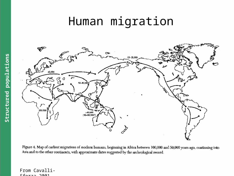
From Cavalli-Sforza,2001

Human migration

Str

uct

ure

d p

op

ula

tio

ns

Th

e C

oal

esce

nt

and

Mea

sura

bly

Evo

lvin

g P

op

ula

tio

ns

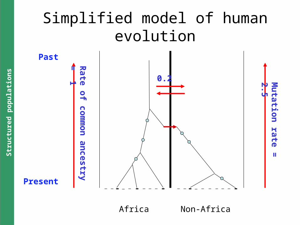
Africa Non-Africa

0.2 Mu

tatio

n ra

te =

2.5

Ra

te o

f co

mm

on

an

ce

stry =

1

Past

Present

Simplified model of human evolution

Str

uct

ure

d p

op

ula

tio

ns

Th

e C

oal

esce

nt

and

Mea

sura

bly

Evo

lvin

g P

op

ula

tio

ns Why Bayesian?

• Probabilistic model-based inference– Can make simple statements about the probability of alternative

hypotheses given the data

• Markov chain Monte Carlo– Convenient computational technique– Allows for complex models: “if you can simulate you can sample”

• Incorporates prior probabilities – P(|D) P(D| )P()– Convenient means of assessing alternative sets of assumptions– Allows incorporation of independent sources of information

• Easy to include sources of uncertainty– Don’t need to assume perfect knowledge of tree (for example)– Can treat the tree and a nuisance parameter and focus on parameters

of interest (strength of selection, mutation rate, growth rate, etc)

Th

e C

oal

esce

nt

and

Mea

sura

bly

Evo

lvin

g P

op

ula

tio

ns Conclusions & cautionary remarks

• Bayesian MCMC has advantages– a useful tool for exploring prior hypotheses– Good for assessing levels of uncertainty– Complex models can be investigated on practical datasets

• Bayesian MCMC has disadvantages– Diagnostics are difficult, and it is essentially impossible to

guarantee correctness– Model comparison can be difficult– Requires large programs that are difficult to optimize and debug.

Th

e C

oal

esce

nt

and

Mea

sura

bly

Evo

lvin

g P

op

ula

tio

ns Conclusions & cautionary remarks (2)

• Population genetics has advantages– provides a framework for objective analysis of genetic data– Allows interpretation of genetic data in terms of biological

properties of virus– Can be extended to include selection, recombination et cetera

• Population genetics has disadvantages– Models are still too simple– Assumptions are too strong– Extending to complex models that include changing selection

pressures and recombination are possible in MCMC but still very difficult!