The Classical-Romantic Dichotomy:A Machine Learning Approach

Chao Peter Yang

A thesis submitted in partial fulfillmentof the requirements for the degree

Bachelor of Science(Honors Data Science)

Supervised byProfessor Edward IonidesProfessor Daniel Forger

Department of StatisticsUniversity of Michigan – Ann Arbor

United States of AmericaApril 08, 2021

Acknowledgements

This paper would not have been made possible were it not for the generous and

formative support of all those involved. First and foremost, I would like to give my

gratitude to Professor Edward Ionides for his guidance on the machine learning part

of this thesis, and Professor Daniel Forger for his help with the analysis of music

using MIDI files. Furthermore, I would also like to thank the researchers and scholars

of the Historical Performance Research group for providing the databases used in

this thesis for the training of the models.

1

Contents

1 Introduction 3

2 Background Information 3

2.1 Support Vector Machines . . . . . . . . . . . . . . . . . . . . . . . . . . 4

2.2 Long Short Term Memory Neural Networks . . . . . . . . . . . . . . . 5

3 Data 6

3.1 Exploration . . . . . . . . . . . . . . . . . . . . . . . . . . . . . . . . . 6

4 Methodology 9

4.1 Conventional Machine Learning . . . . . . . . . . . . . . . . . . . . . . 9

4.1.1 Making of the Data-frame . . . . . . . . . . . . . . . . . . . . . 9

4.1.2 Chord Recognition . . . . . . . . . . . . . . . . . . . . . . . . . 10

4.1.3 Markov Chain . . . . . . . . . . . . . . . . . . . . . . . . . . . . 11

4.2 Neural Networks . . . . . . . . . . . . . . . . . . . . . . . . . . . . . . 12

4.2.1 Data Encoding . . . . . . . . . . . . . . . . . . . . . . . . . . . 12

4.2.2 Data Formatting . . . . . . . . . . . . . . . . . . . . . . . . . . 13

4.2.3 Neural Network Architecture . . . . . . . . . . . . . . . . . . . . 14

5 Results from Conventional Machine Learning Models 15

5.1 SVM Optimization . . . . . . . . . . . . . . . . . . . . . . . . . . . . . 15

6 Results from the LSTM-based architecture 18

6.1 Training . . . . . . . . . . . . . . . . . . . . . . . . . . . . . . . . . . . 18

6.2 Analysis . . . . . . . . . . . . . . . . . . . . . . . . . . . . . . . . . . . 18

7 Conclusion and Future Work 20

2

1 Introduction

The ongoing advancement of subscription services for audio media (YouTube Music,Spotify, Google Music etc.) necessitates the automatic recommendation of differentaudio contents. And with the ever increasing sophistication of the recommendationalgorithms, comes the need for automated Music Information Retrieval (MIR). Forthis paper, we will deal with the musical classification side of MIR.

The literature on musical classification has been focused more on the spec-trum analysis of a given audio file, with notable mainstream classifiers using the spec-tral analysis technique called the MFCC, or the Mel-Frequency Cepstral Coefficients,which is a sort of inverse of the Fourier Analysis [7]. However, these spectral analysistechniques are based on low level information of the sound spectrum, which makes itinapplicable in many situations. For this project, we have decided to use symbolicrepresentations of audio, namely Musical Instrument Digital Interface (MIDI) files, tolook at the mid-level information of the music, such as the chord structure, meter, key,rhythmic make up of the piece, to classify the music. This way, the classifier will haveknowledge of the piece based in music theory, and not just the frequency spectrum.

More specifically, this paper would tackle a more niche aspect of the problem:the classification of Classical and Romantic music using only higher level content.These two eras of music are known for their ambiguous boundaries. If a averagemusically untrained person were to listen to the songs of The Beatles and sonatas ofMozart, they would easily be able to differentiate between the two, and guess thatthe sonatas is classical music, while the songs of The Beatles are some forms of earlypop music. However, even for a relatively well trained classical musician, they wouldstill have a difficult time correctly categorizing an early symphony by Mendelssohn, aRomantic period composer, and a late one by Beethoven, a Classical period composer,especially by looking at the chords only. Indeed, there are those who would questionthe rigor and validity of the Classical-Romantic dichotomy, and a good number ofmusicologists would argue that Beethoven was not actually a Classical period composer[12]. Nonetheless, we will tackle this problem by exploring classification techniques inthe field of conventional machine learning, with a focus on Support Vector Machines(SVMs), and deep learning, emphasizing on the Long Short Term Memory (LSTM)networks specifically.

To this end, we will use MATLAB’s MIDI-Tools package to analyse andprovide the algorithm with the aforementioned mid-level musical data [5]. There arealready implemented functions that could find both the meter and the key of the piecein the package; however, the harmonic components of the analysis will provide moreof a challenge.

2 Background Information

In this paper, we will focus on the use of the Support Vector Machine and the Long-Short Term Memory neural network. Therefore, it would likely be beneficial to clarify

3

the workings of the models in this section

2.1 Support Vector Machines

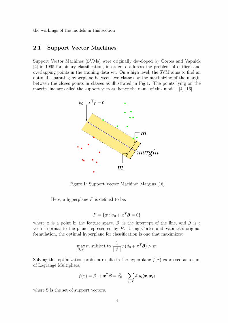
Support Vector Machines (SVMs) were originally developed by Cortes and Vapnick[4] in 1995 for binary classification, in order to address the problem of outliers andoverlapping points in the training data set. On a high level, the SVM aims to find anoptimal separating hyperplane between two classes by the maximizing of the marginbetween the closes points in classes as illustrated in Fig.1. The points lying on themargin line are called the support vectors, hence the name of this model. [4] [16]

Figure 1: Support Vector Machine: Margins [16]

Here, a hyperplane F is defined to be:

F = {x : β0 + xTβ = 0}

where x is a point in the feature space, β0 is the intercept of the line, and β is avector normal to the plane represented by F . Using Cortes and Vapnick’s originalformulation, the optimal hyperplane for classification is one that maximizes:

maxβo,β

m subject to1

||β||yi(β0 + xTβ) > m

Solving this optimization problem results in the hyperplane f(x) expressed as a sumof Lagrange Multipliers,

f(x) = β0 + xT β = β0 +∑i∈S

aiyi〈x,xi〉

where S is the set of support vectors.

4

However, it is important to note that one of the greatly appreciated featuresof the SVM, is its ability to transform the input features via a kernel function when ahyperplane could not effectively classify the data in the original feature space. Withoutthis characteristic, the SVM would do little better than a linear classifier. Instead ofthe inner product, the square of the Euclidean distance, we could replace it with akernel function K that essentially transforms the feature set into a higher dimension.We get

f(x) = β0 +∑i∈S

aiyiK(x,xi).

The only requirement here is that the K has to be symmetric, and positivesemi-definite, since it is replacing the inner product. [16]

2.2 Long Short Term Memory Neural Networks

Although various neural networks could be chosen for our task of the classification ofa chord progression, i.e. a time series, we have chosen the Long—Short-Term Memory(LSTM) networks for its property of being able to retain “memory” of the previouselements in the time series, and not only consider the element that came before thecurrent one. This property of the LSTM network is especially valuable for the analysisof a time series like a chord progression, whose dependencies could span several chords.

A single LSTM layer at time t is defined via the following sets of equations re-formulated by Andrew Ng based on Hochreiter and Schmidhuber’s original formulationin 1997 [8]:

c<t> = tanh(Wc[a<t−1>, x<t>] + bc)

Γu = σ(Wu[a<t−1>, x<t> + bu)

Γf = σ(Wf [a<t−1>, x<t> + bf )

Γo = σ(Wo[a<t−1>, x<t> + bo)

c<t> = Γu ∗ c<t> + Γf ∗ c<t−1>

a<t> = Γo ∗ tanh c<t>

As shown in Fig.2, c<t>, is the input passed in from the previous hidden layer, a<t> isthe variable that records the “state” of the network, and thereby retaining “memory”of the previous elements, and x<t> are the inputs to the current neuron, while theΓu,Γf ,Γo are the update, forget and output gates respectively, with W being theweights matrix, and b the biases.

Noting the complexity of musical chord progressions, we will also use a bi-directional LSTM network, which does not only consider the dependencies of theprevious chords, but also the chords ahead. Illustrated in Fig.3, a bidirectional LSTMnetwork is a stacking of two conventional LSTM networks, one forward and the otherbackwards. Since the predicted y variable is influenced by both the hidden layers thatcame before and after it, it could effectively take into consideration the dependenciesof both directions.

5

Figure 2: LSTM network as illustrated by Raghav Aggarwal [2]

Figure 3: Illustration of a Bidirectinal LSTM network [2]

3 Data

All of the data used in this paper came from the ELVIS Database of the ELVIS Project,and are divided into Romantic and Classical music based on musicological conventions.The files used are all direct representation of the score in the from of MIDI files, witheach movement of the piece being a separate file. As for the assortment of pieces ineach category, we have 394 pieces for the Romantic composers including Tchaikovsky,Chopin, Mendelssohn, Liszt and Grieg. While on the other hand, we have 360 piecesform the Classical era, including Haydn, Beethoven, Schubert, Mozart. Due to theavailability in the Elvis database, Chopin occupies a majority in the Romantic pieces,and the Haydn for the Classical pieces.

3.1 Exploration

For the sake of interpretability, we use the chord labels that would later be betterdefined and explained in the “Chord Recognition” section of the paper to performa simple exploration of the data available. After the chord recognition, the chordalinformation of each piece is encoded as ratios between each chord type and the totalnumber of chords to the data frame, along with the key, meter and the modality ofeach piece, resulting in a 754 by 18 data frame of higher-level musical information tobe used for model training. However, instead of blindly training models, it might bebeneficial to examine the generated data first.

6

Figure 4: Scatter Plot Matrix for Major Pieces

First, by looking at the scatter plot matrix for the major pieces only in Fig.4,we can see that there is, albeit somewhat weak, a visible correlation between the chordsand the class of the piece and the ratio of the chords. This is correlation seems toespecially prominent for the V, ND, and the I chord. Where Romantic pieces seemsto have, in general, a less frequent use of the I and V chord, while having a higherratio of ND chords. This falls inline with the general knowledge of music theory andmusicology, where it is generally understood, that music of the later genre tend to pushthe boundary of diatonic composition through the use of chromaticisms, increasinglyfrequent key-changes and transpositions, and the use of whole-tone scales, all of whichare likely to lead to the classification of a chord to be ND by the chord classificationmethod used in this paper.

This observation, however, does not seem to hold for the minor case. As couldbe seen in scatter plot matrix of the minor chord shown in Fig.5, where the correlationbetween the ratios of the chords and class does not seem to be as strong, so muchso that it is hardly visible from the pair-wise comparison of the scatter plots by thenaked eye. On the other hand, we do see significantly more data points of Romanticpieces for the minor case in Fig.5, suggesting that either there is a correlation betweenthe modality and the class of the composer, or that the data set used might be biased.Indeed out of the 754 samples, 360 are Classical pieces, while 394 are Romantic pieces,with 102 of the Classical pieces being minor compared to the 185 minor pieces for the

7

Figure 5: Scatter Plot Matrix for Minor Pieces

8

Romantic era. However, tempting as it is to assert the correlation between modalityof the pieces and their era, the difference between the numbers could likely come fromuneven sampling of the composers of each era. For the Classical pieces, a large amountof the samples come from Mozart and Haydn, while Tchaikovsky and Chopin, two ofthe more somber characters during the Romantic era, are the two largest contributorto the Romantic samples. Nevertheless, although there might be an inherent biasregarding the composers used for the samples, all of the four composers are known tobe representative of the compositions techniques used of their respective era, thereforethe analysis of the harmonic contents, ie. chords, should remain sufficiently useful.

4 Methodology

4.1 Conventional Machine Learning

This paper could largely be divided into two parts, conventional machine learning anddeep learning. For the machine learning part, we will examine most of the commonlyused classification models ( Logistic, SVMs, Tree etc.) on a data-frame composed ofthe chordal information of pieces. The entire process is as shown in the flowchart ofFig.6. First, a collection of pieces in MIDI files is retrieved from the ELVIS Database,composed of Classical and Romantic pieces are processed by the built-in functions ofthe MIDI-toolbox to extract some of the basic mid-level information of the piece suchas the key, meter, and modality (major/minor) of the piece [5] [13]. Then, the rawdata is fed into a basic chord recognition function (described in detail in section 3.1) toextract the chordal information of the piece. Once the chord progression of the pieceis obtained, the ratio between each chord type and the number of chords is outputtedto the data frame as a number between 0 to 1, while the key, meter and modality ofthe piece is encoded as categorical variables in addition of the true class variable.

After the data-frame is generated, it is used to train most of the well-known,standard classification models with 5-fold cross validation. These are: Decision Trees,Logistic Regressions, Naive Bayes, Support Vector Machines (SVMs) with Linear,Quadratic, Cubic and Gaussian kernels. We then further examine the performance ofthe models after training.

4.1.1 Making of the Data-frame

The generation of the data-frame could be largely separated into three steps:

1. Extraction of the basic Mid-level features such as the Key of the piece usingthe Krumhansl-Schmuckler key-finding algorithm as implemented in the MIDI-Toolbox [5] [14].

2. Cut the piece into frames of a beat or a measure

9

Figure 6: Flowchart for Conventional Machine Learning

3. Run the chord classifying function for each beat with respect to the key, andrecord the chords as a ratio of the total number of chords for the data-frame.

The first step of this sequence is strait-forward, as the Krumhansl-Schmuckler (KS)key-finding algorithm is one of the most often used and relied upon key-finding methodsin MIR research[5]. The KS algorithm constructs a histogram of notes, then categorizesthe piece by key names based on the histogram’s best match with built-in templates.The second step outlines one of our assumptions, that a chord generally does not changemid-beat. Although countless counter examples could be found for this assumption,it does generally hold true for the genres that we examine in this paper, Classicaland Romantic music. The third step is the actual classification of the notes in eachbeat/measure to a chord label.

4.1.2 Chord Recognition

Firstly, the notes from each beat/measure are reclassified into 12 semitone based pitchclass profile (PCP) of C, C#, D, D# etc., represented by integers from 0-11. Then,by taking into account of the key of the piece, we run a chord recognition functionimplemented using the fundamentals of music theory to label the chords. This is anexpert-machine whose working is illustrated via a decision tree as shown in Fig.7.

10

Figure 7: Chord Recognition Function

The input space is an feature vector of pitch-classes to represent the notesof each beat, and another Key-class to represents both the key of the piece andits modality. The function then uses modular operation to determine the differentscale degrees of the using modular arithmetic (ie. Supertonic = (Key + 2) mod 12,Mediant(major) = (Key + 4) mod 12 and so on), and checks for its existence in thefeature vector. The function then deducts which of the basic diatonic chords existingin the scale is the most likely as per the decision tree in Fig.7. If the function is unableto find a suited chord, or there is not enough information, it assumes that the chordis non-diatonic, and “ND” is outputted.

Although other chord recognition models exist that use more advanced clas-sification techniques such Hidden Markov Model (HMM), N-gram models and Convo-lutional Neural Networks (CNN), [7] [3] for the current purposes of this paper, thisrule based identification algorithm is sufficient.

4.1.3 Markov Chain

Noting that since chord progressions are progressions, we do not only need to have theratio of each chords, but also have the need to capture the relationship between the

11

chords. For this purpose, we can use a Markov Chain.

A Markov Chain is a stochastic process that models the transition of a statebased solely on the current state. Named after A.A.Markov, the Markov chain hasseen wide and common usage in the field of artificial intelligence, machine learningand modeling. [9] Simply put, for each stage there is a certain possibility of transitionto another state (or itself). In our case, this would be the transition of chords, asillustrated in Fig.8, where the numbers correspond to the chords in a scale. As couldbe seen, all chords could transition to any chords. Joining the chords in a major scaleand that of a minor scale, we could model an entire Markov Chain via a transitionmatrix P of dimensions 14 by 14 for each piece, with (i, j) being the probability oftransition from i to j. With this in mind, we can flatten this matrix and feed thisinto the data frame for training, resulting in a total of 213 predictors available for thetraining.

Figure 8: Complete Graph of Chords

4.2 Neural Networks

4.2.1 Data Encoding

Since in general, neural networks are more “data-hungry” than other classificationmethods, we should aim to conserve as much of the original data as possible. Thismeans that we could no longer classify all chords into a vocabulary of 14 chords.However, since musical data usually contain many notes at a time, we still have towork with chords nonetheless. Therefore, we will use an encoding method similar toOne-Hot encoding for chords, known as a chroma-vector illustrated in Fig.9.[6] Asillustrated, this is a 12 dimensional vector, with each dimension representing a note ina musical octave. By slicing the music into sections measure by measure, the chroma-vector would encode the notes played by assigning the value 1 to the correspondingnote. Then, we get a time series of chords.

12

Figure 9: A chroma-vector representing a single chord

4.2.2 Data Formatting

To preserve comparability, we use the exact same set of 754 MIDI files for the trainingof our neural network as we have for the previously mentioned methods. However,due to the significantly longer training time for a neural network, using the same 5-fold cross validation technique for the LSTM network is much too impractical for theamount of computational power available for this project. Therefore, we will dividethe data set into 682 training files and 76 test files. Only the training files wouldbe used for the training of the neural network, while the 76 test files would be usedfor validation. This is a stronger test than the 5-fold cross validation used for othermethods, since the test files are never used for the training of the model.

In order to maximize the utility of our limited database, and to fulfill aneural network’s requirement of data with our moderately sized data set of around700 pieces, each piece — ie. chord progression — is split into smaller sequences oflength 50, resulting in around 1500 distinct sequences available for training.

The data is then organized into smaller groups of data known as Mini-batchesto train the neural network each iteration in order to avoid memory overflow.[1] How-ever, since MATLAB’s Deep-learning package requires that the length of the sequencesin a given Mini-Batch to be the same, filler data is added to the shorter sequencesknown as padding. Since padding is filler data and does not add any meaningful infor-mation to the network, it is best minimized. By simply sorting the data by sequencelength, we have achieved that goal as illustrated in Fig.10, where the white spacewithin the red boundaries being the amount of filler needed for each Mini-Batch.

13

Figure 10: Sorted vs Unsorted data

4.2.3 Neural Network Architecture

Considering the complexity of musical chord progressions, the network needs to besufficiently deep in order to capture the patterns and regularities in the data. However,since there are no convention regarding scale needed for such a task, we have opted forthe following design as shown in Fig.11, the scale of which is limited by our availablehardware. Following the sequence input layer is a bidirectional LSTM network with250 layers that outputs a sequence which feeds to a drop out layer to prevent overfitting. This intermediate sequence is then passed to a conventional LSTM network(250) which provides a single output, passing through another dropout layer, to asoftmax function, outputting the classification. The layer numbers here are chosenaccording to the limitation of the graphical computing power available to students atthe CAEN Labs of the University of Michigan.

14

Figure 11: Layers

5 Results from Conventional Machine Learning Mod-

els

The data frame as outputted by the chord classification algorithm is formatted asillustrated in Fig.6, and is used for model training. Models trained include differentgrades of decision trees, logistic regression, Naive Bayes, and Support Vector Machines(SVMs) and different Ensemble methods as shown in Fig.12 and Fig.13.

It could be seen in the figures, that most of the models did not perform well,the Kernel Naive Bayes in particular would have performed better had it just picked’Romantic’ for all of the samples. Two of the most popular methods in classification,decision trees, including the ensemble boosted and bagged trees also did not seem towork particularly well. On the other hand, the various SVM methods, on average,outperformed all of the other classification models.

5.1 SVM Optimization

Since the SVM methods with the Gaussian kernel showed the most promising results,we will attempt to optimize it to obtain a higher accuracy. The function for theGaussian kernel is as follows:

K(x1, x2) = exp

(−‖x1 − x2‖

2

2σ2

)(1)

where x1 and x2 are the two feature vectors, and σ is the width of the kernel, whichin this case is also one of the tuning parameters. Another tuning parameter will be

15

Figure 12: Models trained 1

Figure 13: Models trained 2

the box constraint, the “maximum penalty imposed on margin-violating observations.”There tuning parameters are then optimised using a Bayesian Process for 30 iterations,as illustrated in

Taking a look back at Fig.4 and Fig.5, the suitability of the SVM methodsseems to be more understandable. In Fig.12 and Fig.13, the correlation betweenthe ratios and the classes are minimal, and no clear cut boundaries could be drawnbetween the Classical pieces and the Romantic ones, which would explain the sub-optimal performance of the models other than the SVM. On the other hand, theSVM’s ability to generate new dimensions makes it possible to work around the lowcorrelation between he chord ratios and the class, and draw a boundary hyper-surfaceusing the additional dimension.

Indeed, looking at Fig.15, we see that with an overall accuracy of 73.3%,and a rather even distribution of TPR of 72.8% for Classical pieces, and 73.9% forRomantic pieces, we have produced a respectable accuracy of around 70%, not toofar from some earlier studies for content based musical classifier, with only a rulebased chord classifier, and a well-known SVM classification model, albeit with onlytwo categories. [11]

However, since we have used an optimised SVM, the interoperability of themodel is much worse than optimal; hence, one resorts to looking for correlation betweenthe misclassified data points and the raw data. Yet, unfortunately, we were not ableto find a significant correlation between the misclassified pieces and the composers, orthe length of the piece.

16

Figure 14: Minimum Classification Plot

Figure 15: Confusion Matrix for the Optimized Gaussian SVM

17

6 Results from the LSTM-based architecture

6.1 Training

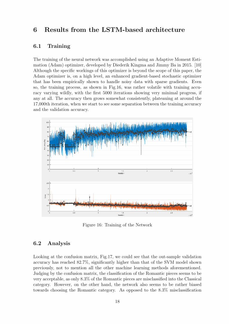
The training of the neural network was accomplished using an Adaptive Moment Esti-mation (Adam) optimizer, developed by Diederik Kingma and Jimmy Ba in 2015. [10]Although the specific workings of this optimizer is beyond the scope of this paper, theAdam optimizer is, on a high level, an enhanced gradient-based stochastic optimizerthat has been empirically shown to handle noisy data with sparse gradients. Evenso, the training process, as shown in Fig.16, was rather volatile with training accu-racy varying wildly, with the first 5000 iterations showing very minimal progress, ifany at all. The accuracy then grows somewhat consistently, plateauing at around the17,000th iteration, when we start to see some separation between the training accuracyand the validation accuracy.

Figure 16: Training of the Network

6.2 Analysis

Looking at the confusion matrix, Fig.17, we could see that the out-sample validationaccuracy has reached 82.7%, significantly higher than that of the SVM model shownpreviously, not to mention all the other machine learning methods aforementioned.Judging by the confusion matrix, the classification of the Romantic pieces seems to bevery acceptable, as only 8.3% of the Romantic pieces are misclassified into the Classicalcategory. However, on the other hand, the network also seems to be rather biasedtowards choosing the Romantic category. As opposed to the 8.3% misclassification

18

rate of the Romantic pieces, the 25.6% misclassification of the Classical pieces doesseem significantly higher.

Figure 17: Confusion Matrix for the LSTM

It is harder to tell much more from the confusion matrix alone, and, dueto the black-box characteristics of the LSTM network, or any neural network for thatmatter, looking into the internal weights and biases would do little to help up interpretthe model either. Therefore, by examining the prediction made with respect to thecomposers of the pieces used in the training, we get more insight into the network.For all the major composers, whose piece is used, we took up to 20 random samplesfor each composers, and recorded the accuracy of the predictions, shown in Fig.18

Interestingly, perhaps not entirely surprisingly, the Classical composers thatreceived the most accurate predictions are those whom one might consider to bequintessentially “Classical,” ie. Haydn and Mozart, who are renowned for their rather“conservative” composing techniques. On the other hand, the composer that scoredthe lowest among the Romantics is Mendelssohn, who, famous and respected thoughhe was, was known for his old fashioned composing techniques and chord progressions.

Should one dig deeper into this, one would see that the network exhibitssimilar behaviours within the compositions of a composer. For example, Schubert’searlier work, Mass 2, D.167 was largely categorized correctly with 4 out of 6 of itsmovements labeled as “Classical.” However, for his later work, the 13 HuttenbrennerVariations, D.576, all of its 13 movements were labeled as “Romantic” without ex-

19

Figure 18: Prediction Accuracy per Author

ception. Likewise, for Mendelssohn’s earlier work, Op19, 3 of its 6 movements werewrongly categorized as “Classical,” while his later Op30 only had 2 of its 5 movementswrongly labeled. His latest work in the data set, Op62 were all categorized correctly.The fact that the network’s prediction coincides so well with one would logically expectgiven one’s musicological understanding of the composers and their composing styles,it is not hard to see that the network might have caught onto something in the chordprogression that is very closely related to the Classical-Romantic dichotomy.

7 Conclusion and Future Work

Needless to mention, the scale of this project is definitely limited, and so is its depth.Although an out-sample accuracy of around 82% has been reach through the LSTMnetwork, and a cross-validated accuracy of 72% for the simpler SVM classifier, thereis no guarantee that this approach would continue to work, should we want to predictmore categories with the model. Recently, some papers have published the use of Con-voluted Neural Networks and Deep Residual Network for chord classification, whichhas a much greater vocabulary than the 14 chord output of the chord classificationmethod used for this paper, and could even function as a noise filter for the chordsequences in the neural net [15] [7]. A more accurate and capable chord classifier likethose would likely be significantly beneficial to this project.

Although this project deals exclusively with MIDI files, it would also beinteresting to see if in the future one could combine the study of mid-level informationsuch as the chord progressions with the analysis of the sound spectrum (low-levelinformation). In this case, we would have a classifier that is trained on both typesof data, MIDI for the chord progressions and such, and audio file for the low levelinformation, and given that the field of sound spectrum analysis has already quite afew works on music classification, it would be interesting to see how the two systemscould work together.

Additionally, although in this experiment, the LSTM network significantlyoutperformed the SVM, there might be some possibility lying in the combination ofthe two, likely a sort of boosted model. As the LSTM network deals exclusively with

20

sequences, adding some higher level information such as the Key, Meter, Tonalityetc. might give a network the necessary additional information, leading to betterpredictions.

References

[1] Long short-term memory networks. Long Short-Term Memory Networks - MAT-LAB Simulink.

[2] Raghav Aggarwal. Bi-LSTM. Medium, Jul 2019.

[3] Nicolas Boulanger-Lewandowski, Yoshua Bengio, and Pascal Vincent. Audiochord recognition with recurrent neural networks. In ISMIR, pages 335–340.Citeseer, 2013.

[4] Corinna Cortes and Vladimir Vapnik. Support-vector networks. Machine learning,20(3):273–297, 1995.

[5] Tuomas Eerola and Petri Toiviainen. MIDI Toolbox: MATLAB Tools for MusicResearch. University of Jyvaskyla, Jyvaskyla, Finland, 2004.

[6] Takuya Fujishima. Real-time chord recognition of musical sound: A system usingcommon lisp music. Proc. ICMC, Oct. 1999, pages 464–467, 1999.

[7] Heng-Tze Cheng, Yi-Hsuan Yang, Yu-Ching Lin, I-Bin Liao, and H. H. Chen.Automatic chord recognition for music classification and retrieval. In 2008 IEEEInternational Conference on Multimedia and Expo, pages 1505–1508, 2008.

[8] Sepp Hochreiter and Jurgen Schmidhuber. Long short-term memory. Neuralcomputation, 9(8):1735–1780, 1997.

[9] John G Kemeny and J Laurie Snell. Markov chains, volume 6. Springer-Verlag,New York, 1976.

[10] Diederik P Kingma and Jimmy Ba. Adam: A method for stochastic optimization.arXiv preprint arXiv:1412.6980, 2014.

[11] Y. Lo and Y. Lin. Content-based music classification. In 2010 3rd InternationalConference on Computer Science and Information Technology, volume 2, pages112–116, 2010.

[12] Dale E Monson. The Classic-Romantic dichotomy, Franz Grillparzer, andBeethoven. International Review of the Aesthetics and Sociology of Music, pages161–175, 1982.

[13] The ELVIS Project. MIDI files of Romantic and Classical pieces, 2020. Dataretrieved from the ELVIS Database, https://database.elvisproject.ca/.

[14] David Temperley. What’s key for key? The Krumhansl-Schmuckler key-findingalgorithm reconsidered. Music Perception, 17(1):65–100, 1999.

21

[15] Y. Wu and W. Li. Music chord recognition based on midi-trained deep featureand BLSTM-CRF hybird decoding. In 2018 IEEE International Conference onAcoustics, Speech and Signal Processing (ICASSP), pages 376–380, 2018.

[16] Zhiwei Zhu. Lecture notes on Support Vector Machines, November 2020.

22