The Chemistry-Forecast Systemat the Meteorological Service of Canada

Richard MénardMeteorological Service of Canada

Global Earth-System Monitoring,ECMWF Seminar, Reading, UK. September 5-9, 2005

Environment CanadaMeteorological Service of Canada

Environnement CanadaService Météorologique du Canada

Canadian Hemispheric and Regional Ozoneand NOx System = CHRONOS

CHRONOS is a CTM used in operational air qualityprediction, data assimilation and real-time scenarios

• 21 km, terrain following heightcoordinate (Gal-Chen) from 0-6 km

• continental domain• ADOM-II chemical reactions• 2 bin PM representation:

PM 2.5 PM 10• gas-phase and heterogeneous

chemistry• aerosol physics:sedimentation

CHRONOS operational version (public)• 1 run/day (00Z) , 48 h forecast• surface ozone objective analysis• predicts O3, PM2.5 mass, PM 10 masshttp://www.msc-smc.ec.gc.ca/aq_smog/aq_guidance_e.cfm

CHRONOS experimental version (ICARTT)• 2 runs/day (00Z and 12Z), 48 h forecast• assimilation of surface O3 observations

CHRONOS real-time scenarios (MSC)• 7 runs/day (00Z), 24 h forecast• On/Off runs for different regions

All US and Canadian emissions Canadian emissions only

http://www.msc.ec.gc.ca/aq_smog/analysis_e.html

Objective analysis and assimilation of surface ozone observations

• Assimilation and objective analysis using the modelCHRONOS

• Objective analysiseach hour, 24/7, year round

• Operational sinceJune 2004

• Multiyear analysessince the summer2002

Alain Robichaud, Richard Ménard, AQMAG team

Global Environmental Multi-scale Air Quality model = GEM-AQ

GEM is the operational meteorology modelwith 4D Var capability• semi-Lagrangian• global/variable (100km) ,

limited area (15 km)• Tropospheric 10 hPa • Stratospheric 0.1 hPa

non-horographic GWDLi and Barker k-correlated radiation

On-line chemistry• Tropospheric chemistry (ADOM-II) with

EDGAR emissions York University• Stratospheric chemisty York University +

BIRA-IASB

Model: GEM-AQ (J. Kaminski and L. Neary, York University, Ontario)Tropospheric chemistry with prescribed surface emissions online with the

operational meteorological model GEM-DM v3.1.23DVAR-CHEM: Y. Yang and Yves Rochon, MSC – Downsview

Chemical tracers analysis added (online) on the operational 3D Varassimilation system MSC-DORVAL)

MOPITT: Canadian instrument (J.Drummond, U of T) (validation V3.0) mounted on satellite EOS-TERRA

Environment CanadaMeteorological Service of Canada

Environnement CanadaService Météorologique du Canada

Online assimilation with operational model GEMRichard Menard, Alain Robichaud,

and Pierre Gauthier

Environment CanadaMeteorological Service of Canada

Environnement CanadaService Météorologique du Canada

Coupled chemical-dynamical data assimilationR. Ménard, P. Gauthier, A. Robichaud, Y. Yang, A. Kallaur,S. Ménard, M. Charron, X. Xie (Meteorological Service of Canada)

D. Fonteyn, S. Chabrillat (Belgium Institute for Space Aeronomy)

J. McConnell, J. Kaminski, L. Neary, J. Jarosz (York University)

•Two year project (ESA) to examine the benefits and drawbacksof chemistry-dynamics coupling in data assimilation

type of coupling: Online , offline, semi-online , multivariate

• 3D and 4D Var assimilation of meteorology and chemistry observationsfrom ENVISAT

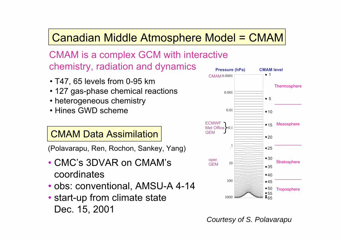
Canadian Middle Atmosphere Model = CMAMCMAM is a complex GCM with interactivechemistry, radiation and dynamics• T47, 65 levels from 0-95 km• 127 gas-phase chemical reactions• heterogeneous chemistry• Hines GWD scheme

• CMC’s 3DVAR on CMAM’s• coordinates• obs: conventional, AMSU-A 4-14• start-up from climate state • Dec. 15, 2001

CMAM Data Assimilation(Polavarapu, Ren, Rochon, Sankey, Yang)

Courtesy of S. Polavarapu

Outline 1. Surface observations- AIRNOW real-time observations- Canadian and US surface observations: current and planned

2. Kalman filtering theory- algorithm- asymptotic stability

3. Optimum interpolation using surface ozone observations- model improvement- implementation- covariance modelling- statistical consistency- verification- background error vertical correlation

4. Other species- why univariate ?- impact of O3 analyses on other species

5. Prediction6. Environmental impact7. How important is chemistry in assimilation and monitoring ?8. Ongoing and future direction9. Some outstanding problems in chemical data assimilation

- unobserved species: analysis, error statistics

~ 40

~ 450

~1300

# Sites CoverageFrequencyUnitsParameter

Limitedhourlyug/m3PM10

Mod-Goodhourlyug/m3PM2.5

GoodhourlyppmOzone

1. Surface observations

Real-time observations : US-Canada

• Available from AIRNOW (US EPA) Data Management Center currently ftp download ASCII files , future BUFR distributed by NOAAcurrently Canadian observations collected at CMC in BUFR

• Data automatically QA/QC’s each hour at US EPA• Available 20-30 min. past the hour

AIRNow Ozone sitesCourtesy: Chet Wayland, US EPA

AIRNow PM2.5 sitesCourtesy: Chet Wayland, US EPA

Meteorological Service of Canada Meteorological Service of Canada

Brewer and ozonesonde sites in Canada

Current measurements5 Flask-sampling sites (CO2, CH4, CO, N2O, SF6, H2, δ13C and δ18O in CO2)4 in-situ measurement sites (CO2, CH4, CO, N2O, SF6 concentrations)1 CO2 flux measurement site

Estevan Point

Alert (GAW)

Prince Albert

Fraserdale

Borden

Sable Island

Canadian Greenhouse GasesCanadian Greenhouse GasesMeasurements Network Measurements Network (MSC)(MSC)

35

7Existing sites

Possible sites planned for EOS(integrated measurements of GHGs and CO2 isotopes with CO2 flux)

# Starting year for vertical profile by NOAA

AEROCAN NETWORK

h

h

h

h

hh

h

h

hhh

Resolute

Saturna IslandBratt’s Lake

WaskesiuThompson

Churchill

Kuujjuarapik

HalifaxKejimkujik

SherbrookeEgbert

hPickle Lake

h

Ft. McMurray

hKelowna

h

Chapais

hNew Sites (2004)hExisting Sites

AEROCAN NETWORK

h

h

h

h

hh

h

h

hhh

Resolute

Saturna IslandBratt’s Lake

WaskesiuThompson

Churchill

Kuujjuarapik

HalifaxKejimkujik

SherbrookeEgbert

hPickle Lake

h

Ft. McMurray

hKelowna

h

Chapais

hNew Sites (2004)hExisting Sites

Repository of monitoring networks (US & Canada)

NATChem www.msc-smc.ec.gc.ca/natchem/index_e.html

AQ, climate and toxics data sets

Future (proposed) of AIRNow (ref Chet Wayland, US EPA)

• US EPA DMC can accept additional parametersprecursor gasesspeciation of aerosolsmeteorological parameters

• Continuous measurements of precursor gases at 24 sitesNO, NO2 (true measurement), NOx, NOy, SO2, CO

• Continuous measurements of aerosols speciation at 10 sitesEC (elementary carbon PM2.5)OC (organic carbon)BC (black carbon)UBV (second channel of Aethalometer)NO3 ions (nitrate)SO4 ions (sulfates)

Prediction

Analysis

an

an

P

xf

n

fn

1

1

+

+

P

x

In a Kalman filter, the error covariance is dynamically evolved between the analyses, so that both the state vector and the error covariance areupdated by the dynamics and by the observations.

( ) 1−+= n

Tn

fnn

Tn

fnn RHPHHPK

( ) fnnn

an PHKIP −=

)( fnnnn

fn

an xHyKxx −+=

ann

fn xMx =+1

nTn

ann

fn QMPMP +=+1

• Prediction

• Analysis

xf,a

Pf,a

tn

tn

observations

2. Kalman filtering theory`

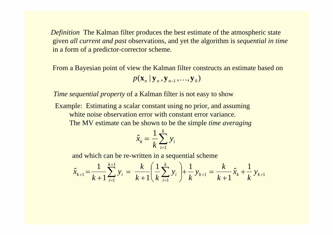
Definition The Kalman filter produces the best estimate of the atmospheric stategiven all current and past observations, and yet the algorithm is sequential in timein a form of a predictor-corrector scheme.

),,,|( 01 yyyx …−nnnpFrom a Bayesian point of view the Kalman filter constructs an estimate based on

Time sequential property of a Kalman filter is not easy to show

Example: Estimating a scalar constant using no prior, and assuming white noise observation error with constant error variance. The MV estimate can be shown to be the simple time averaging

∑=

=k

iik y

kx

1

1ˆ

and which can be re-written in a sequential scheme

111

1

11

1ˆ1

1111

1ˆ ++=

+

=+ +

+=+⎟

⎠

⎞⎜⎝

⎛+

=+

= ∑∑ kkk

k

ii

k

iik y

kx

kky

ky

kkky

kx

a) Asymptotic stability and observability

• We say that we have observability when it is possible for adata assimilation system with a perfect model and perfect observationsto determine a unique initial state from a finite time sequence of observations.

Example: one-dimensional advectionover a periodic domain

0

L

x

L/UT=t

xU

t ∂∂

=∂∂ φφ

continuous observations at a singlepoint x=0 over a time T=L/U determinesuniquely the initial condition φ0(x) = φ(x,0)

Theorem. If an assimilation system is observable and the model is imperfect, , then the sequence of forecasterror covariance converges geometrically to which is independent of{ }f

kP0≠Q

f∞P f

0P

Kalman filter OI and other sub-optimal schemes

observation error observation error

KF analysis error

Forecast error no assimilation

OI

variance evolving

analysis error no assimilation

Results from the assimilation of CH4 observations from UARSMenard and Chang (2000)

The accumulation of information over time is limited by model error, so thatin practice we need to integrate a Kalman filter only over some finite time toobtain the optimal solution

3. Optimum interpolation using surface ozone observations

Motivations

• Tropospheric ozone analysis using an alternative approach toassimilating limb/nadir combination of satellite measurements

• Surface ozone measurements are accurate (<1 ppb), calibrated each night, very small bias, reports each hourin real time, fixed location, extensive spatial coverage.They are ideal to construct error statistics.

• Identify the main model problems, and hopefully correct them.

• To have quickly an operational product, which then helps to take the next step in the development of a comprehensive chemical weather system.

• Air quality analyses and derived quantities (although it may not impact significantly the air quality prediction).

daytime bias : ORIGINAL version

a) model improvement

ORIGINAL version (pre assimilation era) of CHRONOS• bias (red) and error standard deviation (blue) of ~ 20 ppb

and sometime of comparable size no assimilation

Last year (with improvement on clouds, dry deposition, and emissions)• bias (~ 5 ppb, black curve) is smaller than the error standard deviation (green ~ 15 ppb)

Incremental analysis vs cloudCase study. May 02 2004 20Z

In assimilation

• Photochemistry in CHRONOS uses NMP model clouds. • Increase model top in order to better represent clouds in the CTM

What is optimum interpolation ?Approximation to the steady-state Kalman filter

{ }[ ] 1),(),()(

)(−+=

=

RrrBr

K

obsobsobsin

nn

rBiK

iK

)( fnnnn

fn

an xHyKxx −+=

ann

fn xMx =+1

• Prediction

• Analysis

nsobservatio ofpositionofvectorais

pointgridofpositiontheis)nsobservatioofnumber(

dimensionofvectorrowais)pointsgrid

modelofnumber(,,1where

obs

i ir

pK

Ni

r

…=

Remarks:1- Data selection is used to permit the inversion of the innovation

covariance matrix 2- The innovations are generally used to obtain (fit) a functional form of

the background error covariance 3- The background error variances are extrapolated to the whole

model domain

b) Implementation of optimal interpolation

Covariance modelling

Positive definite matrix (Horn and Johnson 1985, Chap 7)

A real n x n symmetric matrix A is positive definite if

for any nonzero vector c. A is said to be positive semi-definite if0>cAcT

0≥cAcT

Properties• The sum of any positive definite matrices of the same size is also

positive definite• Each eigenvalue of a positive definite matrix is a positive real number• The trace and determinant are positive real numbers.

Covariance matrixThe covariance matrix P of a random vector X = [X1, X2, …, Xn]T is the matrixP = [Pij] in which and E is the mathematical expectation.

[ ] [ ]iijjiiij XXXXXXP EE =−−= where))((

Property: A covariance matrix is positive semi-definite

( )[ ]

[ ] 0))((

)()()()(

1,

1,

2111

≥=−−=

⎥⎦

⎤⎢⎣

⎡−−=−++−

∑

∑

=

=

cPcE

EE

Tjjjii

n

jii

n

jijjjiiinnn

cXXXXc

XXcXXcXXcXXc

Remarks1 - It is often necessary in data assimilation to invert the covariance matrices,

and thus we need to have positive definite covariances

2 – The positive definite property is global property of a matrix, and it is nottrivial to obtain

Examples:

a) Truncated parabola⎪⎩

⎪⎨⎧

≤−−

−=otherwise

njiford

jijiC

0

)(1),( 2

2

⎥⎥⎥⎥⎥⎥

⎦

⎤

⎢⎢⎢⎢⎢⎢

⎣

⎡

000.1937.0750.0437.0000.0937.0000.1937.0750.0437.0750.0937.0000.1937.0750.0437.0750.0937.0000.1937.0000.0437.0750.0937.0000.1

for n=4 eigenvalues

0716.00000.00000.02500.18216.3

−

b) Triangle⎪⎩

⎪⎨⎧

≤−−

−=otherwise

njiford

jijiC

0

1),(

⎥⎥⎥⎥⎥⎥

⎦

⎤

⎢⎢⎢⎢⎢⎢

⎣

⎡

000.1750.0500.0250.0000.0750.0000.1750.0500.0250.0500.0750.0000.1750.0500.0250.0500.0750.0000.1750.0000.0250.0500.0750.0000.1

for n=4 eigenvalues

1365.01910.02989.03090.10646.3

Covariance functions (Gaspari and Cohn 1998)

Definition 1: A function P(r,r’) is a covariance function of a random field X if])()(][)()([),( rrrrrr ′−′−=′ XXXXP

Definition 2: A covariance function P(r,r’) is a function that defines positivesemi-definite matrices when evaluated on any grid. That is, letting ri and rj be any two grid points, the matrix Pwhose elements are Pi,j = P(ri,rj) is defines a covariance matrix,when P is a covariance function

The equivalence between definition 1 and 2 can be found in Wahba(1990, p1-2).The covariance function is also known as the reproducing kernel.

Remark Suppose a covariance function is defined in a 3D space, . Restricting the value of r to remain on an manifold (e.g. the surface of a unit sphere)will also define a covariance function, and a covariance matrix (e.g. a covariancematrix on the surface of a sphere)

3R∈r

Correlation function A correlation function C(r,r’) is a covariance functionP(r,r’) normalized by the standard deviation at the points r and r’

),(),()',(),(

rrrrrrrr

′′=′

PPPC

Homogeneous and isotropic correlation function If a correlation functionis invariant under all translation and all orthogonal transformation, then thecorrelation function become only a function of the distance between the twopoints, )(),( 0 rrrr ′−=′ CCSmoothness properties• The continuity at the origin determines the continuity allowed on the rest of the

domain. For example, if the first derivative is discontinuous at the origin, thenfirst derivative discontinuity is allowed elsewhere (see example with triangle)

Spectral representation• On a unit circle

where θ is the angle between the two position vectors, and whereand all the Fourier coefficients am are nonnegative

• On a unit sphere

where all the Legendre coefficients bm are nonnegative.

)cos()(cos),(0

θθ maRCm

m∑∞

=

==′rr

)(cos)(cos),(0

θθ mm

mPbRC ∑∞

=

==′rr

Examples of correlation functions

1. Spatially uncorrelated model (black)

⎩⎨⎧

′≠

′==′−

rrrr

rrif0

if1)(0C

2. First-order auto-regressive model(FOAR) (blue)

⎟⎟⎠

⎞⎜⎜⎝

⎛ ′−−=′−

LC

rrrr exp)(0

where L is the correlation length scale

3. Second-order auto-regressive model(SOAR) (cyan)

⎟⎟⎠

⎞⎜⎜⎝

⎛ ′−−⎟⎟

⎠

⎞⎜⎜⎝

⎛ ′−+=′−

LLC

rrrrrr exp1)(0

4. Gaussian model (red)

⎟⎟

⎠

⎞

⎜⎜

⎝

⎛ ′−−=′− 2

2

0 2exp)(

LC

rrrr

Exercise: Construct a correlation matrix on a one-dimensional periodic domain

Consider a 2D Gaussian model on a plane

22

2

where2

exp),( RL

C ∈⎟⎟

⎠

⎞

⎜⎜

⎝

⎛ ′−−=′ r

rrrr

θr

r’

)cos1(2 22 θ−=′− arr

Along the circle of radius a

Now define a coordinate x along the circle ,

axxaaxx ≤′≤−=−′ ,for2πθ

then we get

⎟⎟⎠

⎞⎜⎜⎝

⎛ ′−−−=′ 2)/(

)]/)(2cos[1(exp),(aL

axxxxC π

x

x’

x

x’

Ways to define new covariances by transformation

Define a new spatial coordinateDefine a new spatial coordinate

If is one - to - one, then

is a new covariance function

x f xQ x x P f x f x

( )( , ) ( ( ), ( ))′ = ′

Linear transformationLinear transformation

If is a linear operator,

then

L xx L x x

T

( )( ) ( ) ( ),µ µ

µ µ

∗ =

=∗P L P L

HadamardHadamard productproduct

If and are two covariance matrices,then the componentwise multiplication

is also a covariance matrix

A B

A B

e gC x y z x y z C x y x y C z zh v

. .( , , , , , ) ( , , , ) ( , )

Separable correlation functions′ ′ ′ = ′ ′ ′

The self - convolution of discontinuousfunctions that goes to zero at a finitedistance, produces compactly -supported covariance functions

SelfSelf--convolutionconvolution

Examples in Gaspari and Cohn (1999)Hadamard product of an arbitrarycovariance function with a compactlysupported function is very useful inEnsemble Kalman filtering to createcompactly supported covariances

State dependenceState dependence

If is a function of the state ,then a state - dependent error

can be used for data assimilation, if in forecast errors

in analysis errors

f

x f x

a

f

µ

ε µ ε

µ µ

µ µ

µ µ∗ =

• =

• =

( ) ( ) ( )

• When formulated this waystate-dependent errors canbe introduced in estimationtheory for data assimilation

e.g. To create a relative errorformulation for observationerror, the relative error isscaled by the forecast interpolatedat the observation location( not the observed value! )

obs – model (obs loc) =

(true + obs error) -(true + model error) =

obs error – model error

2obsσ

)0(2 =xmσ

•

distance (km)

Obs. & background error variances and correlation length scale at

• each sites• each hour

To obtain the error statisticswe use innovations

( )

( )22

2

),()(,

),()()(,))(),((

∑

∑

≠

≠

2Β

−≈

−=

ijBji

ijBBji

jiCiOmFOmF

jiCjiOmFOmFiiLJ

σ

σσσ

1247855320Number of sites

10356777657Observation error

308314334333412

Correlation length scale (km)

297276286279213Forecast error

400332363355 270Total variance

INDUSTRIALAGRICULTURALRESIDENTIALCOMMERCIALFOREST

• Error statistics in terms of land use

• Best fit for correlation model: FOAR (First order autoregressive)

⎟⎟

⎠

⎞

⎜⎜

⎝

⎛ −−=

Lrr

jiC jiexp),(

background error variance - 2Bσ

horizontal correlation length scale - L

),()(),()()(),( obsjiobsjBBobsjiobsjBiBobsji rrCrrrCrrrrB −−−−− ≈= σσσσ

To compute the Kalman gain we have assumed

that the correlation is homogeneous

)( obsjrLL −=

•

•

• and since we perform the full inversion of B + Rwithout data selection

1300≈p

The implementation of an optimum interpolation scheme is actually an iterative process until

jirrBOmFOmF obsjobsiji ≠≈ −− for),(,onassimilatiinputonassimilatioutput

• Pass 0 - No assimilation. Comparison of model simulationwith observations in order to get a first guess onthe error statistics

• Pass 1 - Assimilation using Pass 0 error statistics

• Pass 2 – Assimilation using Pass 1 error statistics

2BσPass 0

2BσPass 1

Pass 0 L

Pass 1 L

Pass 2 - Final

2Bσ 2

Oσ

c) statistical consistency

( ) ( )RB+−2OmF

Monitoring of the error statistics

chichi--squaresquare ( ) pT =+=χ − νν 12 RB

Power spectrum of χ2 gives further insights on theweaknesses of the assimilation system.

• e.g. meteorological analyses are refreshed each 24 hours• e.g. when error stat. were updates each 3 hours we saw

a peak at 3 hours (results not shown)

d) verification

To verify against independent observations we use• 1/3 of observations for the verification (red)• 2/3 of observation used to produce the analysis (blue)• rederive the error statistics (because the background error

may have changed)

e) background error vertical correlation

• The minimum error variance is achieved when the vertical correlation length scale is 900 m – i.e. correlation reaches zerojust above the PBL.

Error statistics during NARSTO 1995 campaign

122 ??690 ??370310Horiz corrlenth

0.220.480.680.72Obs weight

58559860Obs errorvariance

1121194134Forecast Error var

6976292194Totalvariance

July 1995NON=39

July 1995NO2

N=25

July 1995O3

N = 224

August 2002, O3

N=623

4. Other species

Too few observations to construct horizontal error statistics

Impact of assimilating ozone on other species

5. Prediction

ONON OFF ON OFF ON

continuous assimilation

• Dry deposition has an impact on crops and vegetation on a seasonal time scaleAVG. FLUX OF OZONE TO SURFACE : VD*[ozone] – Aug. 7-30 2002

NO O3 ASSIMILATION WITH O3 ASSIMILATION

ppb*m/s ppb*m/s

6. Environmental impact

7. How important is chemistry in assimilation and monitoring

No chemistry

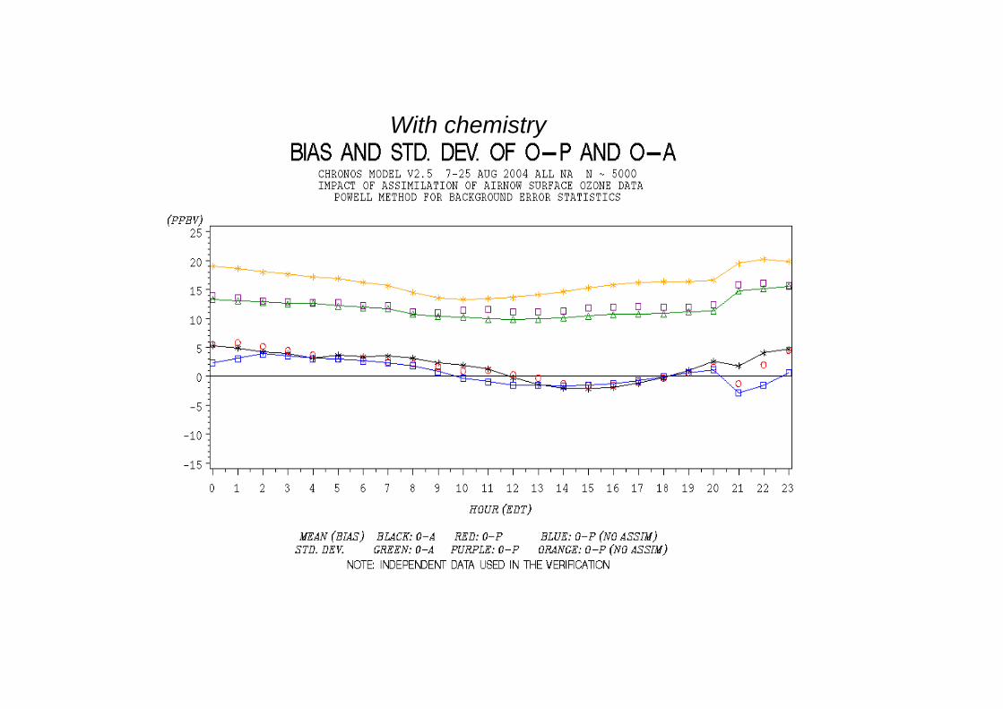
With chemistry

• chemistry + free mode (no assimilation)- std 20 ppb- bias 2 ppb

• no chemistry + assimilation- std ~ 12 ppb- bias a) ~ 1 ppb in analyses

b) large daytime (~10 ppb) in 1hr forecast

• chemistry + assimilation- std ~ 14 ppb- bias ~ 3 ppb (both analysis and forecast)

In summary

Some conclusions

• The reduction of error variance is largest when there is nochemistry. The bias is nearly zero in monitoring mode. The addition of chemistry reduces the effect of observationsi.e. more resilient in reducing the error variance and inadapting the bias.

• The forecast and observation error variances are of comparablesize.

• Reduction of forecast error variance due to surface observationsis about one half.

• The impact of (univariate) assimilation of surface ozoneobservations on prediction last about 3hrs (e-folding time),creating very little corrections on other species.

• the vertical correlation length scale was found by minimizing the forecast error variance. Although barelydetectable (i.e. observability ?), it indicates that correlationshould penetrate just above the PBL.

• surface flux of ozone with/without assimilation of observationsis quite different on a seasonal time scale and may havean impact on the assessment of the environmental impactof ozone

8. Ongoing and future research

• Online chemistry with the operational NWP model GEM (Global EnvironmentalMultiscale model)

• Extend the control variables of the operational 3D and 4D Var to include atmospheric compounds concentrations and surface fluxes.

• Global Environmental Multiscale (GEM) modeloperational NWP model at Meteorological Service of Canadasemi-Lagrangian, adjoint + TLMglobal uniform/variable resolution

• stratospheric versionhybrid vertical coordinate σ → p80 levels, top 0.1 hPa240 × 120 (1.5 degree)

• radiation, k-correlated method (Li and Barker 2004) uses as inputH2O, CO2, O3, N2O, CH4, CFC-11, CFC-12, CFC-113, CFC-114sulfate, sea salt, and dust aerosols.

• non-orographic gravity wave drag (Hines)

Dynamics and physics

data assimilation system• Stratospheric assimilation inherits the characteristics of the operational

assimilation 3D Var and 4D Var– AMSU-A (channel 10-14 added) and AMSU-B microwave channels– GEOS infrared radiances– Data quality control with BG check and QC-Var– Conventional meteorological data

• Extension of operational 3D Var with an arbitrary number of of chemicalspecies

• Chemical species BUFR format proposal to WMO (using IGACO chemicalparameters + other AQ species)

chemistry

• Chemical interface to GEM (next official release)

• Emissions handled through the physics interface (next year)

• Kinetic PreProcessor (KPP) symbolic computation to generateproduction and loss termsjacobian, hessian, LU decomposition matrices.

• Look up J values and online J calculation (MESSy, Landgraf and Crutzen 1998).

• All species advected and gas phase chemistry solved with Rosenbrock or Fully implicit chemical solver (45 min time step).

• Implementation of TLM and adjoint starting this fall.

• Adding surface fluxes as control variables (Next year)

Distributed computing / distributed memory

GCCM OpenMP , MPI VAR-CHEM OpenMP , MPI (underway) , Analysis splitting

Transport

Can save computation in semi-Lagrangian advection transport• upstream point (D or M) is the same for all advected species

x x x

x x x

x x x

• interpolation weights Ci(x) are the same for all advected species

e.g. cubic Lagrange interpolation

Computational Issues

D

MA

∏

∏∑

≠

≠

= −

−== 4

4

4

1 )(

)()( tswith weigh)()(

ikki

ikk

ii

ii

xx

xxxCxCx ϕϕ

Data assimilation issues

• Because the ozone productionrate increases with decreasing temperatures, in regionsdominated by photochemistry(above 35 km) a negativecorrelation between temperatureand ozone would occur

• Haigh and Pyle (1982), Froideveauet al. 1989, Smith 1995, Ward 2002

Cross-error covariance modelse.g. Temperature-Ozone

[ ] ⎟⎠⎞

⎜⎝⎛ Θ=

TBO exp3

• For data at a given level, perturbations can fit an expressionof the form

with a correlation that can be up to 0.92 above 42 km, andincrease linearly from zero to 0.92 between 37 km to 42 km.

• Cross error coupling in 3D Var

[ ][ ] T

Tc

OO δδ

23

3 −=

[ ] [ ] ⎟⎟⎟⎟⎟⎟

⎠

⎞

⎜⎜⎜⎜⎜⎜

⎝

⎛

⎟⎟⎟⎟⎟⎟

⎠

⎞

⎜⎜⎜⎜⎜⎜

⎝

⎛

=

⎟⎟⎟⎟⎟⎟

⎠

⎞

⎜⎜⎜⎜⎜⎜

⎝

⎛

u

suu

u

s

OqpT

IFMI

INIE

I

OqpT

33 lnln

),(

0000000000000000

lnln

),(χψ

χψ

Not all chemical species are observed

Analysis splitting → only observed variables in control vector

The problem of minimizing

with respect to x and u is mathematically equivalent to minimizing

followed by the update (Ménard et al. 2004)

• 4D Var extensionUses same solver as in 3D Var

( ) ( ) ( ))()(21

21),( 1

1

xyRxyuuxxPPPP

uuxx

ux HHJ Tfff

uuf

ux

fxu

fxx

T

f

f

−−+−−⎟⎟⎠

⎞⎜⎜⎝

⎛⎟⎟⎠

⎞⎜⎜⎝

⎛

−−

= −

−

( ) ( ) ( )( ) ( )( )xHyRxHyxxPxxx −−+−−= −− 11

21

21)( Tf

xxTfJ

( ) ( )faxxux

fa xxPPuu −+= −1

( ) ( ) ( )( )( ) ( )( )( )ξξξξξξ LHyRLHy −−+−−= −1

21

21)( TfTfJ ξ

tangent linear integration

End …