the changing value of seniority in the us house...
TRANSCRIPT

The Changing Value of Seniority in the US House:
Conditional Party Government Revised∗
Andrew B. Hall† Kenneth A. Shepsle‡
February 19, 2012
Note to the reader: Additional statistical information, robustness checks, and a description of thedata are available in the Supporting Information, which will be available in an online appendixbefore publication.
∗For comments and advice we would like to thank the participants in the Political Economy Workshop, theAmerican Politics Workshop, and the Graduate Student Political Economy Workshop, all of Harvard University, aswell as the following individuals: John Aldrich, James Alt, Morris Fiorina, Jeffry Frieden, John Marshall, MathewMcCubbins, David Mayhew, Paul Peterson, Sean Theriault, Dustin Tingley, Stanley Veuger, Joachim Wehner, andespecially Anthony Fowler and James Snyder.†PhD Student, Harvard University Department of Government. [email protected]‡George D. Markham Professor of Government, Harvard University. [email protected]
Abstract
In this paper we argue that institutional changes to the seniority system have electoralconsequences to incumbents. Building on the theory of Conditional Party Government, weargue that the consolidation of power in the hands of party leadership reduces the electoralvalue of seniority. This reduction occurs because power that was previously in the hands ofcommittee chairs, whose roles are obtained through seniority, is ceded to party leaders. Wepresent empirical evidence supporting this argument. Our findings suggest that the “condition”of Conditional Party Government, i.e. preference homogeneity among the majority party, is onlya necessary condition; in order for centralization to occur, party reformers must also overcomethe opposition of entrenched senior members. The empirical results suggest that studies ofelectoral outcomes should include institutional variables in their statistical models, and thatstudies of legislative institutions should consider electoral consequences when modeling rulechanges made by legislators.
Word count: 8,058
2

Partly in response to the famous interrogative of Krehbiel (1993) - “Where’s the party?” - a
number of scholars have proposed arguments in which legislative parties play a consequential role
in chamber politics.1 The cartel theory associated with Cox and McCubbins (2007) and the condi-
tional party government theory of Aldrich and Rohde (2001) share the view that parties influence
legislative outcomes through leadership control of institutional arrangements and practices. That
majority leadership impact on legislature proceedings is variable is made especially explicit in the
Aldrich-Rohde theory of conditional party government (CPG, hereafter).
The “condition” part of CPG theory is the degree of homogeneity of policy preferences among
members of the majority party and, a frequent accompaniment, the degree of polarization between
it and the opposition.2 When the majority party coheres around policy, its members “grease the
skids” for the prosecution of the party’s policy agenda by delegating agenda-setting authority and
other powers and resources to their party leaders. In general, that is, “there is a relationship between
chamber CPG and the internal organization of the chamber” (Aldrich, Berger, and Rohde, 2002:
32) or, more concretely, “the greater the degree to which the condition [preference homogeneity
within and preference divergence between legislative parties] is met, the more likely that members
of a party choose to provide their legislative party institutions and party leadership with stronger
powers and greater resources” (Aldrich, Rohde, and Tofias, 2007: 103). Majority party success
in passing commonly supported legislation burnishes the party label and underscores the record
of accomplishment of its members. These are assets when majority legislators next face their
constituents for contract renewal.
The policy preferences of members of the majority party, however, may be heterogeneous -
think the north-south split in the 1940s, 1950s, and early 1960s in Sam Rayburn’s Democratic
majority (lingering on the rest of the 60s and into the 1970s under McCormack and Albert) or
the Tea Party-mainstream conservative split afflicting John Boehner’s Republican majority more
recently. In circumstances such as these, majority-party members are loathe to entrust their leaders
with unchecked discretion. Instead, leaders are made beholden to their caucuses and to their far-
1This literature is summarized by Cox and McCubbins (2005, Chap. 1; 2007).2The CPG literature has not focused much on the extent of preference homogeneity among members of the oppositionparty. Perhaps this is because homogeneity in either party is a function of sorting in the electorate (along withreinforcing redistricting), so that homogeneity in one is often accompanied by homogeneity in the other. We willdevote most of our attention, as does the CPG literature, to the state of the majority party. However, our argumentsuggests some interesting distinctions of CPG’s effect on the majority and minority parties that we examine in thenext section.
3

from-reliable, indeed sometimes irreconcilable, powerful senior colleagues - committee chairs for
Rayburn, factional leaders for Boehner - and have few tools with which to broker consensus.
As a theoretical expectation of CPG theory, then, we should see incumbents of the majority
party (and perhaps the minority party) keen to strengthen party organization and institutional
authority in eras when the “condition” is satisfied, and to decentralize authority in eras when the
“condition” fails. Moreover, we should see incumbents of the majority party benefitting electorally
from these moves in periods in which the condition is met. That is, we should see stronger electoral
advantage for majority-party incumbents in an era of centralized party government. We provide
evidence supporting this view.
But that is not the end of the story. In a strong-party era - one in which central party institutions
and leadership have been strengthened - we uncover a differential effect on electoral benefits among
members of the majority party. In an era of weak party leadership, there is electoral benefit to
seniority. Because senior members dominate committee and party institutions, they are valuable
to their districts and electorally successful as a result.3 The value of seniority, however, declines in
a strong-party era in which, with central party leaders calling the shots, majority-party members
are effectively foot soldiers for, e.g., Newt Gingrich or Nancy Pelosi. That is, while there is a clear
upside for majority-party members in a strong-party era from facilitating the prosecution of their
party’s agenda, the costs of strengthening party institutions are unevenly borne by its members,
afflicting senior members more significantly than junior members. This is our novel revision of CPG
theory, and it, too, is revealed quite clearly in our empirical analysis. Moreover, this diminishing
advantage of seniority in strong-party eras relative to weak-party eras is exclusively a majority-
party affair. No such tax on political capital (seniority) is exacted from members of the minority
party.
These and other empirical expectations are examined in the next section. There we describe
a dataset comprising congressional elections from 1946 to 2008 enabling us to analyze a modified
version of CPG theory. We demonstrate that majority-party leaders endowed with enhanced agenda
power and other institutional authority benefit the majority party rank-and-file, but at the partial
3This assessment is at the heart of a remarkable paper by McKelvey and Riezman (1992), demonstrating that theendogenous creation of a seniority system induces an incumbency advantage - that constituencies, anticipating aseniority system in the next legislative session, will be inclined to re-elect their own incumbent so as not to lose theirdistrict’s “place in the seniority queue.” Seniority attributes, moreover, raise the bar for a successful challenge, thusdiscouraging quality challengers from contesting these seats (Jacobson, 1989).
4

expense of seniors in the majority party. Majority party members may exhibit consensus on policy,
but nevertheless benefit differentially from making the institutional moves to capture the fruits of
this consensus.
Our argument should be seen as fitting into a literature connecting the electoral and legislative
arenas. Too frequently those forecasting congressional elections fail to take on board the impact
of legislative arrangements and political behavior therein. Legislative elections are not dependent
exclusively on national conditions and presidential popularity on election day, but also pivot on
how legislators have conducted themselves, as legislators, in the previous legislative session (see
for example Brady, Fiorina, and Wilkins, 2011). And, in light of this, legislators - especially
majority legislators - arrange institutional practices with a gimlet eye on future electoral contests,
a perspective that goes back to Mayhew (1974), Fiorina (1977, 1989), and their intellectual progeny.
Empirical Strategy and Data
Our goal is to examine the returns to seniority across eras of strong and weak legislative parties.
Our claim is that times of stronger parties should correspond to lower returns to seniority for
majority-party incumbents. To test this claim, we exploit the reforms of the 1970s in the House of
Representatives which, we argue, partition the postwar period into the “Weak Party Era” (1946-
1976) and the “Strong Party Era” (1977-present).
Due to many factors including an increase in party homogeneity, both parties undertook a
series of rule changes in the early 1970s that augmented the power of the party leadership at
the expense of senior members. The majority Democrats in particular assaulted the tradition of
deference to seniority in assigning committee chairmanships. No longer would plum committee
chairmanships belong exclusively to senior members by right; instead, increasing discretion over
committee chairmanships would devolve upon the party caucus and party leadership. The majority
Democrats (and later the majority Republicans) strengthened the party leadership, particularly its
control of the Rules Committee, plenary time, committee assignments, and bill referral.
Shaw (1981: 274) captures the changes clearly: “In various ways traditional norms of deference
were giving way to new arrangements designed to involve junior representatives and senators in
matters previously the concern of senior members.” Discussing these changes to the committee
5

chairmanship selection process, Democratic Speaker of the House Carl Albert declared: “The
seniority system - for sixty-two years the path to legislative domination - died that day...From that
moment on every chairman knew that power flowed not from personal longevity but from the entire
Democratic membership” (as quoted in Remini 2006: 433). The upshot of the reforms was a stark
shift from an era of weak legislative parties, in which committee agenda power and deference to
seniority loomed large, to an era of strong parties, in which party leadership held a far tighter grip
on the reins.4
We take advantage of this historical change by comparing the electoral performance of incum-
bents of differing levels of seniority in the Weak Party Era (WPE) and the Strong Party Era (SPE).
Our main prediction, which we test below, is that seniority is more valuable electorally in the Weak
Party Era, when senior members are able to convert their longevity into more value for their con-
stituents. Because the reforms steadily accumulated through the mid-1970s (Shaw 1981), we take
1976 to be the last election considered part of the Weak Party Era. However, all of the results we
report are robust to moving the end of the Weak Party Era backwards or forwards in time (see
details in the robustness section below).
Data and a First Look
To test our argument, we use a dataset on congressional elections from 1946-2008 that comes from
a series of papers including Ansolabehere et. al. (2010) and Hirano et. al (2010).5 It identifies
representatives by name, district, and year, and contains vote totals for all candidates. Because
we have representatives’ names, we are able to track them over time to determine their seniority,
avoiding problems from redistricting.
Our argument highlights a key shift occurring around 1976 in which seniority began to matter
less within Congress. Since voters care about the value of a representative to the district, we
expect that institutional changes within Congress in the 1970s, reducing the advantages enjoyed by
(and hence the value of) more senior members, have “taxed” those members’ vote shares. These
institutional changes were not exogenous, but rather were brought about by strategic actors who
4Because the Democratic Party was the majority party in the Strong Party Era until 1995, most of the relevantaction occurred in the Democratic Caucus. Of course, in 1995 the Republicans dramatically centralized control intheir leadership.
5The dataset was generously provided to the authors by James Snyder.
6
valued the increased efficiency that a more centralized party offered. The rule changes thus traded
away some of the advantages of more senior members for a party-brand advantage enjoyed by all
members of the party.
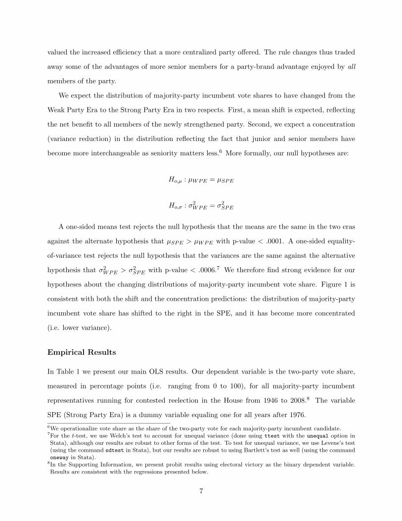
We expect the distribution of majority-party incumbent vote shares to have changed from the
Weak Party Era to the Strong Party Era in two respects. First, a mean shift is expected, reflecting
the net benefit to all members of the newly strengthened party. Second, we expect a concentration
(variance reduction) in the distribution reflecting the fact that junior and senior members have
become more interchangeable as seniority matters less.6 More formally, our null hypotheses are:
Ho,µ : µWPE = µSPE
Ho,σ : σ2WPE = σ2SPE
A one-sided means test rejects the null hypothesis that the means are the same in the two eras
against the alternate hypothesis that µSPE > µWPE with p-value < .0001. A one-sided equality-
of-variance test rejects the null hypothesis that the variances are the same against the alternative
hypothesis that σ2WPE > σ2SPE with p-value < .0006.7 We therefore find strong evidence for our
hypotheses about the changing distributions of majority-party incumbent vote share. Figure 1 is
consistent with both the shift and the concentration predictions: the distribution of majority-party
incumbent vote share has shifted to the right in the SPE, and it has become more concentrated
(i.e. lower variance).
Empirical Results
In Table 1 we present our main OLS results. Our dependent variable is the two-party vote share,
measured in percentage points (i.e. ranging from 0 to 100), for all majority-party incumbent
representatives running for contested reelection in the House from 1946 to 2008.8 The variable
SPE (Strong Party Era) is a dummy variable equaling one for all years after 1976.
6We operationalize vote share as the share of the two-party vote for each majority-party incumbent candidate.7For the t-test, we use Welch’s test to account for unequal variance (done using ttest with the unequal option inStata), although our results are robust to other forms of the test. To test for unequal variance, we use Levene’s test(using the command sdtest in Stata), but our results are robust to using Bartlett’s test as well (using the commandoneway in Stata).
8In the Supporting Information, we present probit results using electoral victory as the binary dependent variable.Results are consistent with the regressions presented below.
7

Distribution of Majority-Party Incumbent Vote Shareby Era
Vote Share (%)
0.00
0.01
0.02
0.03
0.04
20 40 60 80 100
WPESPE
Figure 1 – In this figure we plot the density of majority-party incumbent vote share in the WPE(1946-1976), drawn in black, and in the SPE (1977-2008), drawn in white. The graph shows thatmajority-party incumbent vote share has shifted to the right in the SPE, representing a commonbenefit to all majority-party incumbents, and has also condensed, representing an increase in thesimilarity of majority-party incumbents.
We measure seniority as the number of previous times an incumbent has won reelection. For
example, a two-term representative has a seniority value of 1, since she has successfully run one
previous time as an incumbent.9 To address autocorrelation among repeated observations of the
same incumbent, we cluster all standard errors by representative.
Column (1) corresponds to the following model:
Yit = α+ αSPESPEit + βSSit + βSPE(Sit · SPEit) + εit (1)
Here it indexes representative-year observations (note that we are pooling over t), εit ∼ N(0, σ2i ),
S is our measure of seniority, and Y is vote share. This directly tests our hypothesis that the returns
9This definition may seem odd, but it allows for an easier interpretation of the constant term. Since we are onlyusing incumbents, every observed representative has served at least one term in Congress. We are merely taking thenumber of terms a representative has served and shifting back by one. The constant therefore represents the meanvote share for an incumbent running for her first reelection.
8

Majority-Party Incumbent Vote Share and SeniorityAcross Eras, 1946-2008
OLS Rep Fixed Effects(1) (2)
VARIABLES Vote Share Vote Share
SPE (α̂SPE) 5.51* 0.71(0.64) (0.85)
Seniority (β̂S) 0.83* 0.57*(0.08) (0.10)
Seniority · SPE (β̂SPE) -0.61* -0.65*(0.11) (0.12)
Constant (α̂) 60.84* 64.47*(0.46) (0.46)
Observations 5,940 5,940R-squared 0.05 0.02Number of Fixed Effects 1,842
Standard errors (clustered by representative) in parentheses* p < 0.05
Table 1 – In this table we present our main results. In column (1), we regress vote share onseniority for majority-party incumbents, along with a dummy indicating the SPE (1977-2008), andan interaction of this dummy and seniority. The results show that seniority provides a high returnin the WPE (1946-1976), but a much lower return in the SPE. In column (2), we use fixed effectsfor individual representatives and find a similar result.
to seniority should be lower in the Strong Party Era. βSPE represents the additional vote share
associated with an increase of one in seniority in the Strong Party Era. The overall increase in
vote share associated with an increase of one term of service in the Strong Party Era is therefore
βS + βSPE . Since we are interested in whether the return to seniority changes in the Strong Party
Era, relative to the Weak Party Era, we focus on the sign and the significance level of β̂SPE .
The regression results are consistent with our hypothesis. While an additional term of seniority
in the Weak Party Era is associated with a .83 percentage point increase in incumbent vote share,
an additional term in the Strong Party Era is associated with only a .22 percentage point increase,
a difference that is statistically significant at the .01 level.10
To illustrate, a freshman member of the majority party (an incumbent who has never run as an
incumbent so that S = 0) can expect a vote share in the Strong Party Era of 66.35% (60.84% +
5.51%), whereas she can expect only 60.84% in the Weak Party Era - an SPE premium of 5.51%.
The ability of her party to prosecute its agenda in the Strong Party Era burnishes the party label
10Note that all majority-party incumbents enjoy a boost of 5.51% in vote share in the SPE, independent of seniority- the dividend of a more effective majority party.
9

and provides a dividend - indeed, a non-trivial dividend. As seniority accumulates, a member’s
expected vote share grows, but the size of the SPE dividend shrinks and ultimately turns negative.
Thus, a four-term member (S = 3) expects a 67.01% vote share in the Strong Party Era (60.84%
+ 5.51% + 3 (0.22%)) and 63.33% in the weak party era (60.84% + 3 (0.83%)), yielding an SPE
dividend of 3.68%. Compared to the freshman, a four-term member expects a larger vote share
(67.01% v. 66.35%) but a smaller dividend (3.68% v. 5.51%) in the Strong Party Era. An eleven-
term member (S = 10) in the Strong Party Era expects a vote share of 68.55% compared to 69.14%
in the Weak Party Era - a negative dividend of -0.69%. The value of seniority in the Weak Party
Era, when large enough, exceeds the value of being a senior member of a strong majority party.
This pattern of results requires a reinterpretation of conditional party government, something we
develop further in the discussion section.
In column (2), we add fixed effects for individual representatives. This strategy controls for
unobserved differences across representatives. The results show that even within a given majority-
party incumbent’s career, the switch to the new party regime is associated with a significant re-
duction in the return to seniority.11
In the above regressions we use majority-party incumbent vote shares in contested elections.
We are not including incumbents who run unopposed, or who choose not to run.12 It is well known
that these factors trouble many estimates of incumbency advantage (see for example Gelman and
King, 1990). However, because we are looking at the difference between two eras, these omissions
should not affect our result. It is not our goal to estimate the incumbency advantage, but rather
to show that, among incumbents, the returns to seniority have diminished in the Strong Party Era.
In our main specification, we employ a linear model as a good first approximation of the return
to seniority. It is reasonable, however, to suspect that the relationship between seniority and vote
share is non-linear, with gains to seniority accruing faster in earlier terms. A sophomore legislator
might see her vote share increase markedly in her second reelection attempt compared to her first,
but it is unlikely that John Dingell gains significant vote share between, say, his 25th and 26th
terms of service. Alford and Hibbing (1981) provide evidence for this form of relationship. With
11It is worth noting that, while the coefficients appear to suggest that the seniority effect here, β̂S + β̂SPE , has gonenegative, this sum is not significantly different from zero (p = .35). The attenuation of α̂SPE in the fixed-effectsmodel likely results from only estimating it using members whose careers span the two eras.
12Our results are robust to the inclusion of uncontested elections, where incumbents are coded as receiving 100% ofthe vote share.
10
the advantage of 27 additional years of data, we are able to confirm this non-linearity and compare
returns across our two eras.
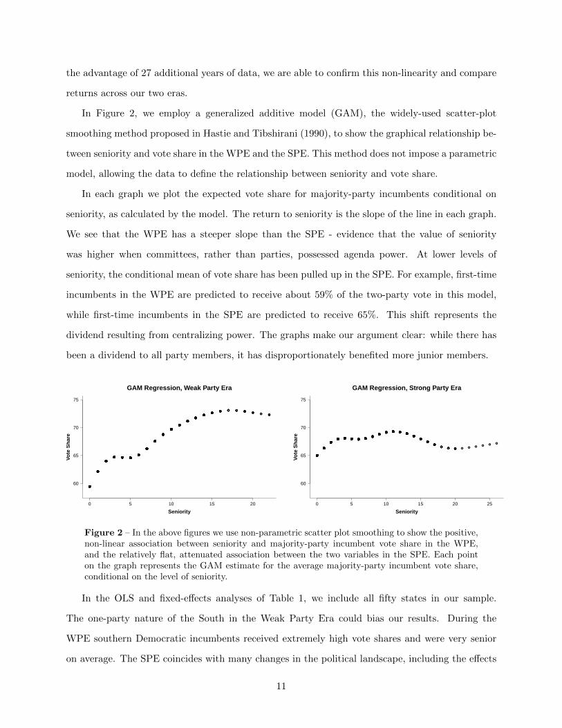
In Figure 2, we employ a generalized additive model (GAM), the widely-used scatter-plot
smoothing method proposed in Hastie and Tibshirani (1990), to show the graphical relationship be-
tween seniority and vote share in the WPE and the SPE. This method does not impose a parametric
model, allowing the data to define the relationship between seniority and vote share.
In each graph we plot the expected vote share for majority-party incumbents conditional on
seniority, as calculated by the model. The return to seniority is the slope of the line in each graph.
We see that the WPE has a steeper slope than the SPE - evidence that the value of seniority
was higher when committees, rather than parties, possessed agenda power. At lower levels of
seniority, the conditional mean of vote share has been pulled up in the SPE. For example, first-time
incumbents in the WPE are predicted to receive about 59% of the two-party vote in this model,
while first-time incumbents in the SPE are predicted to receive 65%. This shift represents the
dividend resulting from centralizing power. The graphs make our argument clear: while there has
been a dividend to all party members, it has disproportionately benefited more junior members.
●
●● ●
●
●
●
●
●
●
●●
●
●
●
●
●
●
●●
●
●
●
●
●
●
●
●●
●●
●●
●
●
●
●●
●
●
●
●●
●
●
●●
●
●
●
●
●
●
●
●
●
●
●●
●●
●
● ●
●●●●●
●
●
●
●
● ●
●
●
●●
●
●
●
●●
●
●
●
●
●
●
●
●
●●
●● ●
●
● ●
●
●
●
●
●
●
●
●●
●
●
●
●
●
●
●●
●●●
●
●
●
●
●
●
●
●
●
●
●
●
●
●
●
●
●
●● ●
●
●●
●
●
●
●●
●
●
●
●
●
●
●
●
●
●
●
●
●●●
●
●
●
●
●
●
●
●
●
●
●
●
●
●
●
●
●
●
●●
●
●
●
●
●●
●
●
●
●
●
●
●
●
●
●
●
●
●
●●
●
●
●
●●
●
● ● ●
●
●
●
●●
●
●
●●
●
●●●
●
●
●
●
●
●
●
●
●●
●
●
●
●
●
●
●
●
●●●
●
●
● ●
●
●
●
●●●
●
●●●●
●
●
●
●●
●
●●
●
●
●
●
●
●
●
●
●
●
●
●●
●
●●
●
●
●
●
●
●
●
●
●
●●
●●
● ●
●
●●
●●
●
●●●
●
●
●●
●
●
●
●
●
●
●●
●
●●
●
●●
●
●
●●
●
●
●●
●●●●
●
●
●
●
●●●
●
●
●
●
●
●
●
●
●
●
●
●
●
●
● ●
●
●●
●
●
●
●
●
●
●
●
●
●
●
●
●
●●●
●
●
●
●
●●
●
●
●
●● ●
●
●
●
●
●
●
●●
●
●
●●
●
●
●
●
●●●
●●
●
●
●
●
●
●
●
●
●
●●
●
●●
●
●
●
●●
●
●
●
●
●
●●
●
●●
●
●
●
●
●●●
●
●
●●
●
●
●
●
●
●
● ●
●●●●●
●
●
●
●●●●●
●
●●
●
●●●●
●
●●●
●
●
●
●
●
●
● ●
●
●
●
●
●
●
●
●●●
●
●● ●
●
●
●
●
●●
●
●
●
●
●
●
● ●
●●
●
●
●
●
●●●
●
●
●
●
●●
●
●
●
●
●
●
●
●
●
●
●
●
●
●
●
●
●
●●
●●●
●
●
●
●●
●●
●
●
●
●
●
●
●
●
●
●
●
●
●
●
●
●●
●
●
●
●
●
●
●●●
●
●●●
●
●
●
●
●
●
●
●●
●
●
●
●
●
●
●
●
● ●
●
●
●●
●
●
●
●●●
●
●
●
●
●
●
●
●
●
●●
●
●
●
●
●
●
●
●
●
●
●
●
●
●
●
●
●
●
●
●
●
●●
●
●
●
●
●
●
●
●
●
●
●
●
●
●
●
●
●●
●●●
●
●●
●
●
●●
●●
●
●
●
●
●●●
●
●
●
●
●●
●
●●
●
●●●
●
●●
●
●
●●
●
●
●●
●● ●
●●
●
●
●
●●
●●
●
●
●
●
●
●
●
●
●
●
●
●
●
●
●
●
●
●
●
●
●
●
●
●
●
●
●
●
●●
●● ●
●
●
●
●
●
●
●●
●
●
● ●
●
●
●
●●●
●
●
●
●
●
●
●
●
● ●
●
●
●●●
●
●
●
●
●
●
●
●
●
●
●
●
●
●
●
●
●
●
●●
●
●
●
●
●
●
●
●●●
●
●
●
●
●
●
●
●
●●
●
●
●
●
●
●
●
●●
●
●
●
●
●
● ●
●
●
●
●
●
●
●
●
●
●●
●
●
●
●
●
●●
●
●
●
●
●
●
●
●●
●● ●
●
●
●
●
●
●
●
●
●
●
●
●●●
●
●
●●
●
●
●
●
●
●
●
●
● ●●
●
●
●
●
●
●
●
●
●
●
●
●
●
●
●
●●
●
●●
●● ●●
●●●
●●● ●●
●
●
●
●
●
●
●
●
●●
●
●
● ●
●
●●
●
●
●
●
●
●
●
●●
●●
●
●
●
●●
●
●
●
●
●
●●
● ●●
●
●
●
● ●
●
●
● ●
●
●
●
●
●
●●
●
●
●
●
●
●
●
●
●
●
●
●
●
●
●
●●
●
●
●
●
●
●●
●
●
● ●
●●●
●●
●
●
●
●
●
●
●
●
●●
●
●
●
●
●
●
●
●
●
●
●●●
●
●
●●
●
●
●● ●●
●
●
●
●
●
●
●
●
●
●
●
●
●●
●
●
●
●
●●
●
●
●
● ●
●
●
●
●
●
●
●●●
●
●●
●
●
●
●
●
●
●●
●
●
●
●●
●
●●
●
●● ●
●●
●
●
●
●
●
●
●
●
●
● ●
●●
●
●
●●
●●
●
●
●●
●
●
●
●
●
●
●●●
●
●
●
●
● ●
●
●
● ●
●
●
●
●
●
●
●
●
●●●
●
●
●●
●
●
●
●
●
●
●
●●●
●
●
●●
●
●
●
●
●
●●
●●
●●
●
●
●
●
●
●
●●
●
●
●
●
●
●
●
● ●
●
●
●
●
●
●
●
●
●
●
●
●●
●
●●
●
●
●
●
●
●
●
●
●
●
●
●●
●
●
●
●
●
●●
●
●
●
●●
●●
●
●●●
●
●
●
●
●
●
●
●●
●
●●
●
●●●
●
●
●
●
●
●
●●
●●●
●●
●
●
●
●
●
●
●
●
●
●
●
●
●
●
●●
●●
●
●
●
●
●
●
●
●
●●●
●
●
●
●
●
●
●
●●
●
●
●
●
●
●
●
●
●
●
●
●
●
●●
●
●●
●●
●●
●●
●
●
●
●
●
●
●●
●
● ●
●
●
●
●
●
●
●
●
●
●
●
●
●
●
●
●●●
●
●
●
●
●
●
●
●
●
●
●
●●●
●
●●
●
●
●
●
●
●
●● ●
●
●
●
●
●
●
●
●
●
●
●●
●
●
●
●● ●
●
●
●
●
●
●
●
●
●
●
●
●
●
●
●
●
●
●
●
●
●
●
●●
●
●
●
●
●
●
●
●●●
●
●
●●
●
●
●
●●
●
●
●
●
●●
●
●
●
●●
●
●
●
●
●●
●
●
●
●●
●
●
●
●
●●
●
●●
●●
●
●
●
●
●
●●
●
●
●
●
●
●
●
●
●
●
●
●
●●
●
●
●
●
●
●
●
●
●
●
●●
●
●
●
●
●
●
●
●
●
●
●
●
●●
●
●● ●
●
●
●
●●
●
●
●
●
●
●
●
●●
●
●
●
●
●
●
●
●
●
●●
●
●
●
●
●
●
●
●
●
● ●
●
●
●
●
●
●●
●
●●
●
●
●
●
●
●●
●
●
●
●
●
●
●
●
●
●
●●
●
●
●
●●●
●
●
●
●
●
●●
●
●
●
●
●
●●
●
●
●
●
●
●
●
●
●●●
●
●
●
●
●
●
●●
●
●
●
●
●
●
●●
●
●●
●
●
●●
●
●
●
●
●
●
●
●
●
●
●
●
●
●
●
●
●
●
●
●
●
●
●
●
●
●
●
●
●
●●●
●
●
●
● ●●
●
●
●
●
●
●
●
●
●
●
●
●
●
●
●
●
●
●
●
●
●●
●
●
●
●
●
●
●
●
●
●
●
●
●●
●
●●
●
●●●
●
●
●
●
●
●
●●
●
●
●●●
●
●
●
●
●●
●
●
●
●
●
●
●
●●●●
●
●●
●●
●
●
●
●
●
●
●
●
●
●
●●
●
●
●
●
●
●●
●
●
●
●
●●
●●
●
●
●
●
●
●
●
●
●
●
●
●
●
●
●●
●
●
●
●
●
●
●
●
●
●
●
●
● ●
●
●
●●●
●
●
●
●
●
● ●●
●
●●
●
●
●
●
●
●
● ●
●
●
●
●
●
●
●
●
●
●
●
●●
●
●
●
●
●
●●
●
●●●●
●●
●
●
●
●
●
●
●●●
●
●
●
●
●●
●
●
●
●
●
●
●
●
●
●
●
●●●
●
●
●●●
●
●
●
●●
●
●
●
●
●
●
●●
●●
●
●
●
●
●
●●
●
●
●●●●
●●
●
●
●
●●
●
●
●
●
●
●
●●●●
●
●
●
●●
●
●●
●●●
●
●
●
●
●
●
●
●●
●
●
●
●
●
●
●
●
●●
●
●
●
●
●
●
●
●
●
●
●● ●
●
●
●
●
●●
●
●
●
●
●
●
●
●
●
●
●
●
●
●
●
●
●
●
●
●
●
●●
●●●●
●●
●
●●
●
●
●
●
●
●
●
●●
●
●
●
●
●
●
●
●
●
●
●●
●
●
●
●
●
●
●
●
●
●
●
●
●●
●
●
●●
●
●
●
●
●
●
●
●
●
●
●
●
●
●● ●
●
●
●
●
●
●
●
●
●
●
●
●
●
●
●
●
●●
●
●
● ●
●
●
●
●
●
●
●
●
●
●●●
●
●
●●●
●
●
●●
●
●
●
●
●
●●●●●
●
●
●
●
●
●●
●
● ●
●●
●
●
●
●
●
●
●● ●
●
●
●
●
●
●●
●
●
●
●
●
●
●
●
●
●●
●●
●●
●
●
●
●
●
●
●
●
●
●
●
●
●
●
●
●
●
●
●
●
●
●●●●
●
●
●
●
●
●
●
●
●
●
●
●
●
●
●
●
●
●
●●
●
●
●
●●
●
●
●
●
●●
●●
●
●
●
●
●
●
●
●
●
●
●●
●
●
●
●●
●
●
●●●
●
●●●
●●
●
●
●●
●
●
●
●
●
●
●
●
●
●
●
●
●●
●
●
●
●
●●
●
●
●
●
●
●●
●
●
●
●
●
●
●
●
●
●
● ●●●
●
●
●●
●
●
●
●
●
●
●
●
●●
●
●
●
●●
●
●
●●
●
●
●●● ●●●●
●
●
●
●
●
●
●
●
●●
●
●●
●
●
●
●
●
●
●
●
●
●
●
●
●
●
●
●
● ●
●
●
●
●
●
●
●
●
●
● ●
●
●
●
●
●
●
●●
●
●●●
●
●
●
●
●
●
●
●
●
●
●
●
●●
●
●
●
● ●
●
● ●
●
●
●
●
●
●
●
●
●●
●
●
●
●
●
●
●
●
●
●
●
●
●
●
●
●
●
●
●●
●
●
● ●
●
●
●
●
●●
●
●
●
●
●
●
●
●
●
●
●
●●
●
●
●
●
●
●
●
●
●
●
●
●
●●
●
●
●
●
●
●
●
●
●
●
●●
●
●
●
●
●
●
●
●
●
●
●
●
●
●
●
●
●
●
●●
●
●
●
●
●
●
●
●
●
●
●
●
●
●
●
●
●
●
●
●●
●
●
●
●
●
●
●●
●
●
●
●
●
●
●
●
●
●
●
●
●
●
●
●
●
●
●
●
●
●
●
●
●
●
●
●
●
●
●
●
●
● ●
●
● ●
●
●
● ●
●
●
●●
●
●
●●
●
●
●●
●
●●
●
●
●
●
●
●
●
●
●
●
●
●
●
●
●
●
●
●
●
●
●
●
●
●●
●
●●
●
●
●
●
●●
●●
●
●
●
●
●●
●
●
●●
●
●
●
●●
●
●
●
●
●●
●
●
●
●●
●
●
●
●
●
●
●
●
●
●
●
●
●
●
●
●
●
●
●
●
●
●
●●
●●
●
●
●
●●
●
●●●
●
●
●
●
●
●
●
●
●
●
●
●●
●
●
●
●
●
●
●
●
●
●
●
●
● ●
●
●
●
●
●
●●
●
●
●
●
●●
●
●●●●
●
●
●
●
●
●
●
●
●
●
●
●
●●●
●
●
●●●
●
●
●
●
●
●●
●
●
●
●
●
●
●●
●
●
●●
●
●
●●
●
●
●●
●
●●
●
●●
●
●●
●●
●
●
●
●
●
●
0 5 10 15 20
Seniority
Vote
Sha
re
60
65
70
75
GAM Regression, Weak Party Era
● ●
●
●
●
●
●
●
●
●
●
●
●
●
●
●
●●
●
●
●● ●
●
●
●●
● ●●
●
●
●
●
●
●
●
●
●
●
●
●
●●
●
●
●●
●●
●
●●
●
●●
●
●●
●
●●
●
●●●●●
●
●
● ●●
●●
●
●●
●
●
●
●
●
●●
●●
●
●
●
●
●●
●●
●
●
●
●●
●
●●
●●
●
●●
●
● ●
●
●
●
●
●
●
●
●
●
●●
●
●
●
●
●
●●●
●
●
●
●
●
●
●●
●
●
●
●
●
●
●
●
●
●
●
●
●●
● ●
●
●
●
●● ●●
●
●
●
●●
●
●●
●
●
●●
●
●●
●●
●
●
●
●
●●
●
●●
●
●
●●●●●
●
●
●
●●●●●●●●
●
●
●
●
●
●
●
●
●
●
●
● ●
●
●●
●
●
●
●
●
●
●●
●
●
●
●
●
●●
●
●
● ●
●●
●
●●
●●
●●
●●
●
●
●●
●●●
●
●●
●
●
●
●
●
●
●
●
●
●●●
●
●
●
●
●
●●
●
●
●
●
●
●
●
●
●
●
●
● ●
●
●
●
●
●
●
●
●
●
●
●
●
●
●●●
●●
●
●
●
●
●●
●
●
●
●
●
●
●
●
●
●
●
●
●
●
●
●
●●
●
●
●
●
●
●
●
●●
●
●●
●
●
●●
●
●●
●
●
●
●
●
●
●
●
●
●
●
●
●●●
●
●
●
●
●
●
●
●●
●
●
●
●
●●
●●
●●
●
●
●
●●
●
●
●
●●
●
● ●
●
●
●
● ●
●
●
●
●
●
●
●
●
●
●●
●
●
●
●
●
●
●
●
●
●
●● ● ●
●
●
●●
●
●●
● ●
●●
●
●
●●
●
●●
●
●
●●
●
●
●
●
●
●
●●
●
●
●
●
●●
●
●●
●
● ●
●
●
●
●
● ●
●
●
●
●
●
●
●
●
●
●
●
●
●
●
●
●
●
●
●●
●
●
●
●●
●
●● ●●
●
●
●
●
●
●
●
●
●●
●
●●
●
●
●
●
● ●
●
●
●
●
●●● ●
●
●●
●
●
●
●
●●
●
●
●
●
●
●●
●●
●
●
●
●
●
●
●
●●
●●
●●
●
●
●
●
●
●●
●
●
●●
●●●
●
●
●
●
●● ●●●
●●
●
●● ●
●
●
●
●
●
●
●
●
●
●●
●
●
● ●
●
●
● ●
●
●●
●
●
●●●
●
●
● ●
●
● ●●
●
●
●
●
●
●
●●
●
●
●
●
● ● ●●
●
●
●
●
●
● ●●
●
●
●
●
●
●
●●
●
●
●
●●
●●
●
●
●
●
●●
●
● ●
●
●
●
●
●
●●
● ●
●
●
●
●
●●
● ●
●●
●
●
●
●
●
●●●● ●
●
●
●●
●
●
●●
●
●
●
●
●
●
●
●
●●
●
●
●
●
●●
●
●● ●
●
●
●
●
●
●
●●
●
●
●●
●
●●
●
●
●
●
●
● ●●
●
●
●●●
●
●
●
●
●●
●
●
●
●
● ●
●
●
●●
●
●
●
●
●
●
●
●
●
●
●
●
●
●
●
●
●●
● ●
●
●
●
●●
●
●
●●● ●●
●
● ●● ●●
●
●●
●●●
●
●
●
●
●
●
●
●●
●
●●
●
●
●
●
●●
●● ●●
●
●
● ●●
●
● ●● ●●
●●
●
●
●
●
●
●●●
●
●
●
●
●●
●
●●●●
●
●
●● ●
●●
●
●●
●
●
●●
●
●
● ●
●
●
●●
●●
●
●
●
●●
●
●
●
●●●
●
●
●●●
●
●
●
●
●
●● ●●● ●
●
●
●
●
●
●
●●
●
●
●
●●
●●
●
●
● ●
●
●
●
●
●
●
●● ● ●● ●
●
● ●
●
●●●
●●
●
●
●
●
●
●●
●
●
●
●
●
●
●●
●
●●
● ●
●
●
●●
●
●
●
●
●●●●
●●
● ●●
●
●
●●
●
●●
●
●
●
●
●
●
●
●
●
●
●
●
●●
●●
●
●
●
●●●
●
●●
●●●
●
●
●
●
●●
●
●
●●● ●
●
●●
●
●
●●
●●
●
●●
●
●
●
●
●
●
●
●
● ●
●
●
●
●
●
●●
●
●
●
●
●●
●
●
●
●
●●
●●
●
● ●
●
●
●
●
●
●
●●
●●●
●
●
●●
●
●
●
●●
●
●
●
●●
●
●
●● ●●●
●
●
●
●●●
●●
●
●
●●
●
● ●
●
●
●
●
●●
●
● ●●
●●●
● ●
●
● ●●
●
●
●
●
● ●●●● ●●
●●●
●●●
●
●
●
●
●
●
●
●
●
●
●
●●
●
● ●●●
●
● ● ●● ●●
●
●
●● ●●
●
●
●
●
●●
●
● ● ●●
●
●
●● ●● ●
●
●●
●
●
●
●●
●
● ●● ●
●
●
●
●
●
●
●
●●
●●
●
●
●● ●
●
● ●
●
●
● ●●
●
●
●
●●
●
●
●
●
●
●
●
●
●
●
●
●
●
●● ●●
●
●
●●
●
●●
●●● ●
●
●
●
●
●
●●
●
●
●
●
●●
●
● ● ●●
●
● ● ●● ●
●
●
●
●●
●
●
●
● ●●●
●
●●●●
●
●
●●●
●
●
●●
●
●
●
●
●
●
●
●
●
●
● ●
●●
●
●
●
●
●●
●
●
●
●
●●
●
●
●
●●●
●
●
●●
● ●●●● ●
●
●●
●
●●●
●
● ●
●
●
●
●●
●
●
●
●
●
●●●
●
●
●
●
●
●●
●
●
●
●
●
●
●●
●
●●
●
●
●
●
●
●
●
●
●
●●
●
●
●●
●
●
●
●
●
●
●
●
●
●●
●
●●
●●
●
●
●
●
●
●
●
● ●
●●
● ●
●
●●
●
●
●
●
●●
●
●
●
●
●
●
●●●
●
●
●
●
●●
●
●●
●
●
●
●
●
●
●
●
●●●●
●
●
●
●
●
●
●
●
●
●
●●
●
●
● ●●
●
●
●
●
●
●
●
●
●
●
●
●
●●
●
●
●
●
●
●
●●
●●
●●
●
● ●
●●
●
●
●
●
●●
●
●●
●
●
●●
●
●
● ●
●
●
●
●
●
●
●
●
●
●
●
●
●
●●●
●●
●
●
●●●●
●
●
●
●
●
●
●
●
●●
●
●
●
●
●
●
●
●
●
●
●
●● ●
●
●
●
●
●
●
● ●●
●
●
●
●●
●
●
●
● ●
●
●
●
●
●
●
●●
●
●
●
●
●
●
●
●
●
●
●
●●
●
●
●
●
●
●
●●
●
●
●
●
●
●
● ●
●
●●
●●
●
●
●
●●●
●●
●
●
●
●
●
●●
●●
●●●
●
●
●
●●
●
●
●
●●
●
●
●
●●
●
●
●
●
●
●●
●
●●
●●
●
●
●
●●
●
●
●
●
●
●
●
●
● ● ●●
●
●●●
●
●
●
●
●
●
●●
●
●
●●
●
●
●●
●
●●●
●
●
●
●
●●
●
●
●
●
●
●●
●
●
●
●●
●
●
●
●●
●
●
●
●●●●●●●
●
●
●●
●
●
●
●
●● ●
●
●
●
●
●
●
●
●
●
●
●●
●
●
●●
●
●
●
●
●
●
●
●
●●●●
●
●●
●
●●●
●●
●
●
●
●
●
●
●●
●
●
●
●
●
●●
●
●
●●
●●
●
● ●
●
● ●●
●
●●
●
●
●●
●●●●
●●●●●
●
●●
●●
●
●
●
●
●
●
●
●●●
●
●
●●●●
●
●
● ●
●
●
●
●●
● ●●
●
●
●●
●
●●
●
●●●
●●
●
●
●
●
●
●●
●
●
●
●
●●
●
●
●
●
●
●
● ●
●●●
●●
●
●
●
●
●
●
●
●
●
●●
●
●
●
●
●●
●
●●
●
●
●
●
●●
●
●
●
●
●
●
●
●●
●
●
●●
●
●
●
●●●
●
●●
●
●
●
●
●
●
●
●
●●
●
●
●●
●
●
●
●●
●
●●●●
●● ●
●
●
●●
●
●
●●
●
●
●
●
●
●
●
●
●
●
●
●
●●
●
●
●
●
●
●●
●
●
●
●
●●●●
●
●
●
●
●●●
●
●●
●
●
●
● ● ●●●
●
●●
●●
●
●●
●
●
●
●
●
●
● ●
●
●
●
●
●●
●● ●● ●
●
●
●
●
●●
●
●
●
●
●
● ●●
●
●
●●
● ●
●●
●
●●
●●●
●
●
●
●
●
●
●
● ●●
●
●
● ●
●
●
●● ● ●
●
●
●
●
●●
●
●
●
●
●
●●
●
●●
●
●
●●
●
●
●
●
●
●
●
●
●●
●
●
●
●
●●
●
●
●
● ●●●
●
●
●
●
●
●
●● ●
●
●
●●
●
●
●
●
●●●
●
●
●
●●
●
●
●
●
●
● ●●
●
●●
●●
●
●●
●
●
●
●
●●
●
●●
●
● ●
●
●●●●
●
●●
●
●
●
●●
●
● ●●
●●●
● ●
●
●
●
●
●
●●
●
●
●
● ● ●
●
●
●
●
●
●
●
●
●
●
●
●●
●
●● ●
●●
●●
●
●
●
●
●●● ●●●●
●
●
●
●● ●●●
●
●●●●●
●
● ●
●
●
●●
●
●●
●
●
●
●
●
●
●
●
●
●
●
●
●●
●
●
●
●
●●
●
●●
●
●
●
●
●
●
●
●
●
●
● ●●
●
●
●
●
●● ●●● ●● ●● ●●●
●
●
●
●
●
●●● ●
●
●
●
●
●
●●●
●●
●
●
●
●
●●
●
● ●
●
●
●●●
●
●
●●
●
●
●
●
●
●
●
●
●
●
●
●
●●●
●
●
●
●
●●
●
●
●
●
●
●●
● ●
●
●
●
●
●
●●●●
●
●●
●
●
●
●
●
●
●
●
●
●
●
● ●●
●
●
●
●
●
●●●
●
●●●
●
●
●●
●
●●
●
●● ●
●
●
● ●
●
●●
●●
●
●●
●●●●
●
●
●●
●
●
●
●
●
● ●
●●●
●
●●
●
●
●●●●
●
●
●
●●●
●
●
● ●
●
●
●
● ●
●●●●
●●
●
●
●
●
●●
●
●
●●
● ● ●●
●
●●
●
●●
●
●
●
●●●● ●
●●
●
●●●●
●
● ●
●
●● ●●●●
● ●
●
●
●●
●
●●
●
●
●
●
●●
●
●
●
●
●
●
●●
●
●●
●
● ●
●●
●●
●
●
●● ●
●
●
●
●
●
●
●
●●
●
●
●
●
●● ●
●●
●
● ●●●
●
●
●
●
●●
●
●●
●
●
●
●
●●
●
●
●
●
●
●
●
●
●
●
●
●●
●
●
●● ●
●
●
●
●
●●
●
●
● ●
●
●
●
●●
●
●
●
●
●
●
●●
●
●●
●
●
●
●
●
●
●●
●
●●
●
●
●
●
●
●
●
●●
●
●
●
●
●
●
●
●
● ● ●●●
●
●
●
●
●●● ●● ●
●
●●●●
●
●
●
●●●
●●
●●
●
●
●●
●
●
●
●
●
●
●●●
●
●
●
●● ●●
●
●●
●
●
●
●
●●
●
●
●
● ●
●
●
●
●●
●
●
●
●
●
●
●
●●
●
●
●
●
● ●
●●●
●●
●
●
●●●●
●
●
●
●●
●
●
●
●
●
●
●
●●● ● ●● ●
●
●
●
●
●
●
●● ●● ●●●
●
●
●
●●
●
●
●
●
●
●
●
●
●●
●
●●●
●
●
●
●
●
●●
● ●
●
●
●
●
●
●
●
●
●
●
●
●
●
●
●
●
●
●
●
●
●
●
●
●
●
●
● ●
●
●
●
●
●
●
●
●
●●
●
●●● ●
●
●
●
●●
●
●●
●
●
●
●
●
●
●
●●
●
● ●●●
●
●●
●
●●●●●●
●
●
●●
●
●
●
●
●
●●
●
●
●
● ●
●
●
●●
●
●● ●
●
● ● ●●
●
●●●
●
●●
●
●
●
●●
●
●●
●
●●
●
●
●●
●● ●
●●
●
●
●●
●
●
●
●
●
●
●
●
●
0 5 10 15 20 25
Seniority
Vote
Sha
re
60
65
70
75
GAM Regression, Strong Party Era
Figure 2 – In the above figures we use non-parametric scatter plot smoothing to show the positive,non-linear association between seniority and majority-party incumbent vote share in the WPE,and the relatively flat, attenuated association between the two variables in the SPE. Each pointon the graph represents the GAM estimate for the average majority-party incumbent vote share,conditional on the level of seniority.
In the OLS and fixed-effects analyses of Table 1, we include all fifty states in our sample.
The one-party nature of the South in the Weak Party Era could bias our results. During the
WPE southern Democratic incumbents received extremely high vote shares and were very senior
on average. The SPE coincides with many changes in the political landscape, including the effects
11

of the Voting Rights Act of 1965. If the ultimate effect of the Voting Rights Act were harm to
southern Democratic incumbents’ vote shares, the decline in the importance of seniority we observe
more generally could be driven by the southern states rather than by our proposed explanation.
Alternatively, our finding could stem from safe southern Democratic districts in the WPE turning
into safe Republican districts in the SPE. Because the majority party in our study is almost always
the Democratic party, our results could come from ignoring southern incumbents in the SPE. To
address these and other possible concerns about the southern states, we re-run the analysis from
Table 1 using only northern states. As seen in Table 2, our result is stronger when restricted to
northern incumbents.
Northern Majority-Party Incumbent Vote Share andSeniority Across Eras, 1946-2008
OLS Rep Fixed Effects(3) (4)
VARIABLES Vote Share Vote Share
SPE (α̂SPE) 7.04* 0.76(0.77) (0.99)
Seniority (β̂S) 1.01* 0.93*(0.10) (0.09)
Seniority · SPE (β̂SPE) -0.79* -0.89*(0.13) (0.13)
Constant (α̂) 58.86* 62.55*(0.51) (0.47)
Observations 3,981 3,981R-squared 0.08 0.05Number of Fixed Effects 1,227
Standard errors (clustered by representative) in parentheses* p < 0.05
Table 2 – In this table we reproduce our main results, restricting the sample to only non-southernstates. In column (3), we regress vote share on seniority for majority-party incumbents, alongwith a dummy indicating the SPE (1977-2008), and an interaction of this dummy and seniority.The results show that seniority provides a high return in the WPE (1946-1976), but a much lowerreturn in the SPE. In column (4), we use fixed effects for individual representatives and find asimilar result.
Trends in the Returns to Seniority
We have presented evidence that the average return to seniority for majority-party incumbents is
lower in the Strong Party Era than in the Weak Party Era. In this subsection, we address two
12

concerns about our empirical strategy: we show that our finding is not the result of one or two
strange elections, and that it is not caused by a trend in voting behavior over time.
In Figure 3, we report the results of a cross-sectional regression of vote share on seniority for
each year in our dataset. Specifically, for each year we run the regression Yi = α + γSi and plot
the estimate γ̂. The figure shows that all but two years in the Weak Party Era exhibit returns to
seniority higher than the Strong Party Era mean. It confirms that the difference in the average
return to seniority between the two eras, which β̂SPE measures in earlier tables, is not the result
of one or two negative shocks but is instead a relatively consistent change.
Return to Seniority by Year (γ̂)
−0.4
0
0.4
0.8
1.2
1.6
'46'48
'50
'52 '54'56
'58
'60
'62
'64
'66
'68
'70
'72
'74
'76
'78 '80 '82
'84
'86
'88
'90 '92 '94
'96
'98
'00
'02 '04'06
'08
SPE Mean
WPE SPE
Est
imat
ed E
ffect
Figure 3 – In this figure, we graph the return to seniority by year. Each bar represents γ̂ in aregression Yi = α+γSi for year t, i.e. a cross-section regression of vote share on seniority in a singlecongress. The results suggest a persistent decrease in the returns to seniority in the SPE: only twoyears in the WPE exhibit returns to seniority at or below the mean return for years in the SPE.
Another concern with our measure of the change in the average return to seniority is that we
might be picking up a trend in voter behavior. If voters are becoming more “anti-seniority” over
time, for example, we might observe a decrease in the returns to seniority that is unrelated to
13

institutional factors.13 To address this issue, we replicate Table 1 using the minority party instead
of the majority party. The results in Table 3 show that there is no decrease from the WPE to
the SPE in the average return to seniority for the minority party, i.e. β̂SPE is not negative. This
table provides compelling evidence that voters are not simply becoming more anti-seniority over
time. (Indeed, the average minority incumbent’s seniority contributed positively to vote share in
the SPE.)
Minority-Party Incumbent Vote Share and SeniorityAcross Eras, 1946-2008
All States North(7) (8)
VARIABLES Vote Share Vote Share
SPE (α̂SPE) 4.96* 5.24*(0.67) (0.81)
Seniority (β̂S) 0.17 0.12(0.09) (0.10)
Seniority · SPE (β̂SPE) 0.19 0.29(0.13) (0.15)
Constant (α̂) 62.31* 62.00*(0.45) (0.52)
Observations 4,743 3,571R-squared 0.07 0.08
Standard errors (clustered by representative) in parentheses* p < 0.05
Table 3 – In this table we rerun our main specification (from Table 1) restricting the sample tominority-party incumbents. In column (7) we include all states, and in column (8) we exclude thesouthern states. In both cases, we find no reduction in returns to seniority for the minority party.
Polarization as an Alternative Explanation
Because of the necessarily crude nature of our analysis - comparing returns across two time periods
- we can never precisely identify either the change in the returns to seniority or the change in the
average majority-party incumbent vote share caused by the congressional reforms of the 1970s.
However, we can marshall evidence suggesting that our story is more consistent with the data than
are alternative explanations.
Consider the case of polarization. A significant body of work in political science examines the
growing polarization of American politics (see for example McCarty et. al., 2006). Much of the
13“Anti-seniority” could be reflected in complaints about so-called “career politicians.”
14
evidence we have presented so far may also seem consistent with an increase in partisan polarization.
Increased polarization leads to more partisan voting behavior. Voting on a wholly partisan basis
reduces the returns to seniority; as polarization increases, voters attach more weight to party label
than to other characteristics such as seniority, specific policy goals, or even candidate quality.
Polarization and its electoral consequences will affect both parties. If polarization explains the
majority party’s reduction in the returns to seniority, we should see the same phenomenon in the
minority party. However, as Table 3 showed, returns to seniority for the minority party, positive in
the WPE, do not attenuate in the SPE (and in fact increase, if anything).
Furthermore, polarization should affect all facets of American politics. If polarization drives our
empirical findings, then we might expect to find the same reduction in the returns to seniority, and
accompanying strong-party “bump,” in other areas. In Table 4, we replicate our empirical strategy
using the US state senates, state assembly houses, and the US Senate. Because the datasets for
these three legislative bodies do not extend far enough back to generate accurate estimates for the
seniority levels of 1940s legislators, we use legislator fixed effects in all three cases. The results
are clearly at variance with those found above in our analysis of the US House of Representatives.
Majority-party incumbent legislators in the states have seen somewhat positive mean-shifts in vote
share since 1976, but have seen no real changes in the returns to seniority. The US Senate, which
we might think is the best control case for the US House, sees a large decrease in average vote share
and no change in the returns to seniority.14 Overall, the results seem to demand a House-specific
explanation like the one we provide, rather than an explanation based on a macro political force
like polarization, which we would expect to affect a wide range of institutions (an expectation
unfulfilled).
14It is worth noting that institutional change in the US Senate undermining seniority was well underway in the1950s and 1960s. These include the decline in the apprenticeship norm and the adoption of the Johnson Rule(facilitating the appointment of junior senators to top committees). The increasing Senate workload, additionally,made it necessary to rely on junior members, another development occurring during mid-century decades beforethe so-called “strong party era” in the House. This is not to say that everything happened in the Senate beforethe SPE. For example, the election of committee chairs in the Senate, and the more equitable allocation of staff(S.Res. 60), occurred in the 1970s. For details, see Ornstein, Peabody, and Rohde (1977) and their updates in thethe three subsequent editions of Congress Reconsidered.
15

Placebo Tests Using Other Chambers
State Houses State Senates US Senate(1) (2) (3)
VARIABLES Vote Share Vote Share Vote Share
SPE (α̂SPE) 0.37 4.21* -9.21*(0.65) (1.27) (3.42))
Seniority (β̂S) -0.23 -0.09 -1.13(0.23) (0.52) (1.15)
Seniority · SPE (β̂SPE) -0.05 -0.70 1.29(0.24) (0.54) (1.40)
Constant (α̂) 65.23* 62.91* 66.69*(0.50) (0.99) (1.64)
Observations 20,630 5,754 427R-squared 0.00 0.02 0.06Number of Fixed Effects 9,872 3,096 254
Standard errors (clustered by representative) in parentheses* p < 0.05
Table 4 – In this table we replicate our main analysis on three other legislatures: US state assemblyhouses, US state senates, and the US Senate. We do not find a consistent result across thesechambers, suggesting that our findings on the House are not the result of macro-level phenomenain the United States over the same time period.
Minority Party and Returns to Seniority
Because it is the majority party that can directly influence procedure and thereby affect the returns
to seniority, we have largely restricted our analysis to majority-party incumbents. We can now
investigate whether the returns to seniority are different for majority and minority members. In
the Weak Party Era, we might expect that the returns to seniority by and large accrue to members
of the majority party, since it is the majority party that controls the committees. In the Strong
Party Era, when parties rather than committees hold power, we might expect seniority to matter
less in both parties.
To investigate these hypotheses, we specify a new model which we estimate in Table 5:
Yit = γ + γMMinit + γSSit + γSM (Minit · Sit) + εit (9)
Here Min is a dummy variable equaling one if the candidate is a member of the minority party.
γSM represents the return to seniority for members of the minority party, benchmarked against
returns to seniority for members of the majority party.
16
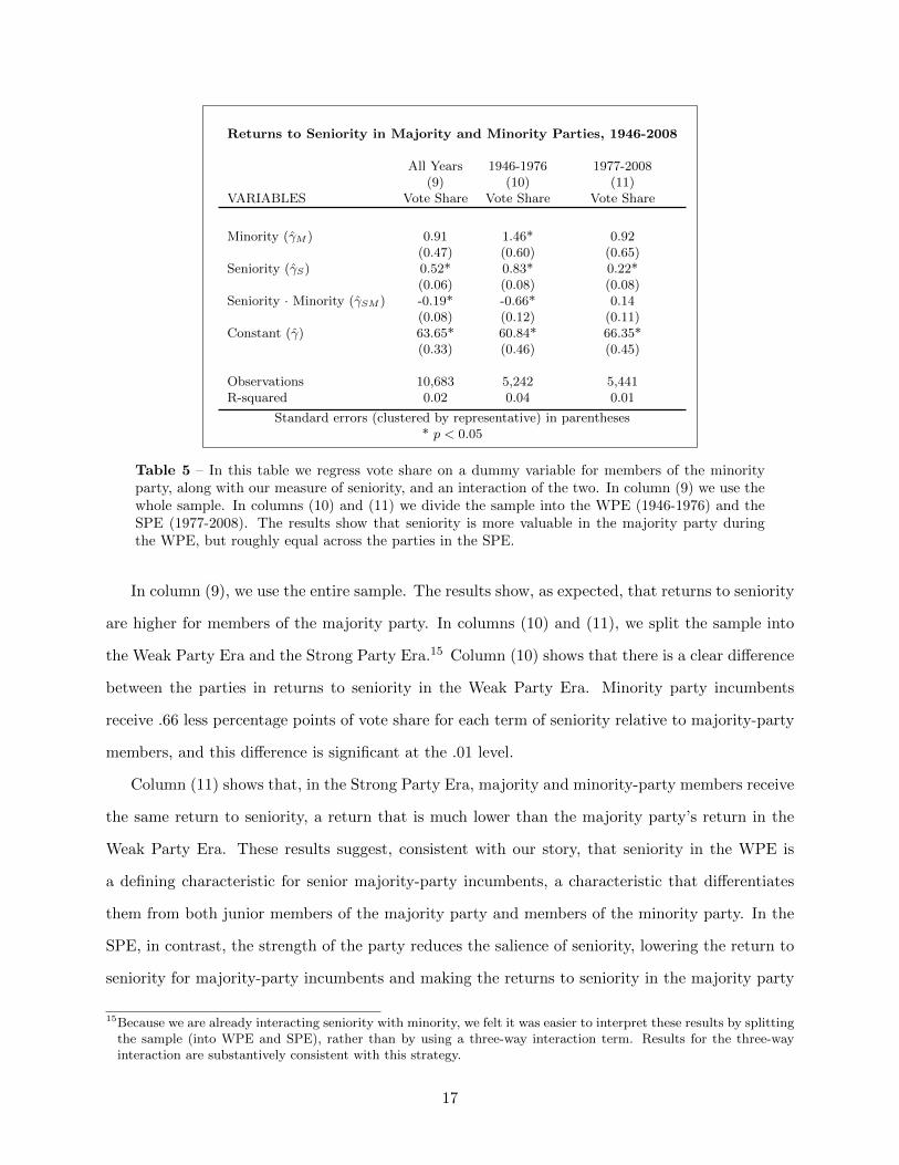
Returns to Seniority in Majority and Minority Parties, 1946-2008
All Years 1946-1976 1977-2008(9) (10) (11)
VARIABLES Vote Share Vote Share Vote Share
Minority (γ̂M ) 0.91 1.46* 0.92(0.47) (0.60) (0.65)
Seniority (γ̂S) 0.52* 0.83* 0.22*(0.06) (0.08) (0.08)
Seniority · Minority (γ̂SM ) -0.19* -0.66* 0.14(0.08) (0.12) (0.11)
Constant (γ̂) 63.65* 60.84* 66.35*(0.33) (0.46) (0.45)
Observations 10,683 5,242 5,441R-squared 0.02 0.04 0.01
Standard errors (clustered by representative) in parentheses* p < 0.05
Table 5 – In this table we regress vote share on a dummy variable for members of the minorityparty, along with our measure of seniority, and an interaction of the two. In column (9) we use thewhole sample. In columns (10) and (11) we divide the sample into the WPE (1946-1976) and theSPE (1977-2008). The results show that seniority is more valuable in the majority party duringthe WPE, but roughly equal across the parties in the SPE.
In column (9), we use the entire sample. The results show, as expected, that returns to seniority
are higher for members of the majority party. In columns (10) and (11), we split the sample into
the Weak Party Era and the Strong Party Era.15 Column (10) shows that there is a clear difference
between the parties in returns to seniority in the Weak Party Era. Minority party incumbents
receive .66 less percentage points of vote share for each term of seniority relative to majority-party
members, and this difference is significant at the .01 level.
Column (11) shows that, in the Strong Party Era, majority and minority-party members receive
the same return to seniority, a return that is much lower than the majority party’s return in the
Weak Party Era. These results suggest, consistent with our story, that seniority in the WPE is
a defining characteristic for senior majority-party incumbents, a characteristic that differentiates
them from both junior members of the majority party and members of the minority party. In the
SPE, in contrast, the strength of the party reduces the salience of seniority, lowering the return to
seniority for majority-party incumbents and making the returns to seniority in the majority party
15Because we are already interacting seniority with minority, we felt it was easier to interpret these results by splittingthe sample (into WPE and SPE), rather than by using a three-way interaction term. Results for the three-wayinteraction are substantively consistent with this strategy.
17
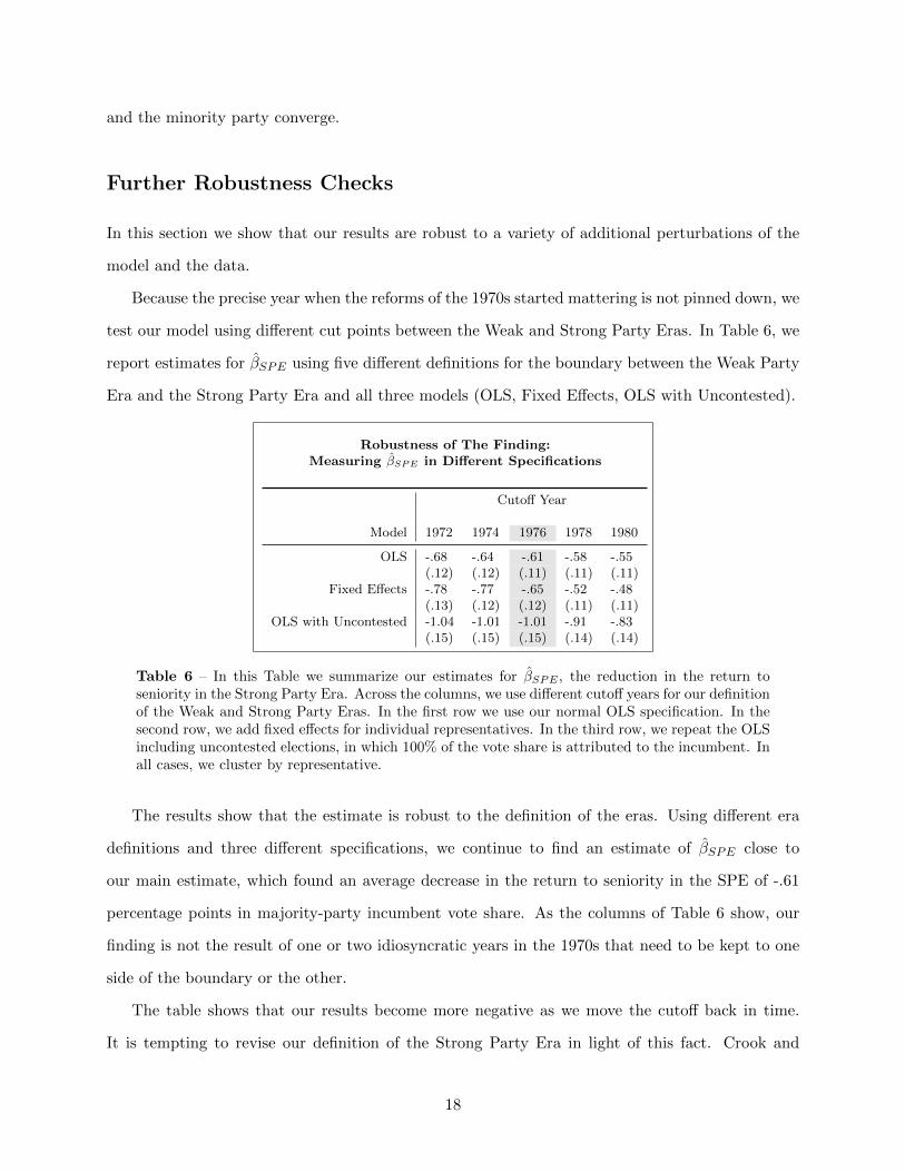
and the minority party converge.
Further Robustness Checks
In this section we show that our results are robust to a variety of additional perturbations of the
model and the data.
Because the precise year when the reforms of the 1970s started mattering is not pinned down, we
test our model using different cut points between the Weak and Strong Party Eras. In Table 6, we
report estimates for β̂SPE using five different definitions for the boundary between the Weak Party
Era and the Strong Party Era and all three models (OLS, Fixed Effects, OLS with Uncontested).
Robustness of The Finding:Measuring β̂SPE in Different Specifications
Cutoff Year
Model 1972 1974 1976 1978 1980
OLS -.68 -.64 -.61 -.58 -.55(.12) (.12) (.11) (.11) (.11)
Fixed Effects -.78 -.77 -.65 -.52 -.48(.13) (.12) (.12) (.11) (.11)
OLS with Uncontested -1.04 -1.01 -1.01 -.91 -.83(.15) (.15) (.15) (.14) (.14)
Table 6 – In this Table we summarize our estimates for β̂SPE , the reduction in the return toseniority in the Strong Party Era. Across the columns, we use different cutoff years for our definitionof the Weak and Strong Party Eras. In the first row we use our normal OLS specification. In thesecond row, we add fixed effects for individual representatives. In the third row, we repeat the OLSincluding uncontested elections, in which 100% of the vote share is attributed to the incumbent. Inall cases, we cluster by representative.
The results show that the estimate is robust to the definition of the eras. Using different era
definitions and three different specifications, we continue to find an estimate of β̂SPE close to
our main estimate, which found an average decrease in the return to seniority in the SPE of -.61
percentage points in majority-party incumbent vote share. As the columns of Table 6 show, our
finding is not the result of one or two idiosyncratic years in the 1970s that need to be kept to one
side of the boundary or the other.
The table shows that our results become more negative as we move the cutoff back in time.
It is tempting to revise our definition of the Strong Party Era in light of this fact. Crook and
18
Hibbing (1985) suggests using 1970 as the cutoff in a similar analysis, arguing that the reforms of
the mid-70s were already anticipated by 1970 in Washington DC.16 This definition of the end of the
WPE in fact generates the strongest possible result for our specification (moving any farther back
before 1970 begins to attenuate the result). However, we believe it is prudent to continue to use
1976. This is a more conservative cutoff which keeps the Watergate election in the WPE, biasing
us against finding a result.
To test whether our cutoff is particularly meaningful, we carry out a Monte Carlo permutations
test. We randomly sample 16 years of our data to assign to a “placebo” WPE, and assign the
remaining 16 to a simulated “SPE.” Using these new era assignments, we re-run our main speci-
fication (column 1 in Table 1) and store the coefficients. We repeat this procedure 10,000 times.
We find that Table 1’s estimate for α̂SPE , 5.51, is larger than over 99% of the estimates from the
permutation test. Likewise, we find that our estimate for β̂SPE , -.61, is smaller than over 99% of the
simulated values. The histograms in Figure 4 display these findings graphically. In each histogram,
the small region shaded in black represents simulated values more extreme than those estimated
in our regressions. Both black regions contain less than 1 percent of the simulated density. The
test suggests that the era division we have proposed is meaningful, and that the differences we find
between the two eras are not replicable under a large number of other ways to split the data.
16This cutoff is perhaps more reasonable in the case of Crook and Hibbing (1985) because it is a story about thebehavior of representatives and not voters. The former might reasonably be expected to anticipate reform earlierthan the latter.
19

Monte Carlo Permutations for α̂SPE
0
100
200
300
400
500
600
−6 −4 −2 0 2 4 6
Monte Carlo Permutations for β̂SPE
0
100
200
300
400
500
−0.5 0.0 0.5
Figure 4 – Above are histograms from the simulations for the SPE intercept (α̂SPE) and for the
SPE change in the return to seniority (β̂SPE). The simulations come from Monte Carlo permuta-tions tests in which years are randomly assigned to the WPE and SPE, respectively. The regionsshaded in black show the simulations producing values more extreme than those found in our mainspecification. More than 99% of simulated coefficients are in the gray area, i.e. less extreme thanour estimates.
20
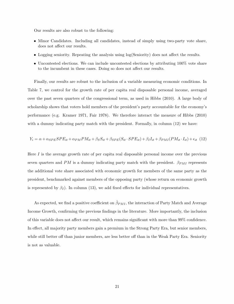
Our results are also robust to the following:
• Minor Candidates. Including all candidates, instead of simply using two-party vote share,does not affect our results.
• Logging seniority. Repeating the analysis using log(Seniority) does not affect the results.
• Uncontested elections. We can include uncontested elections by attributing 100% vote shareto the incumbent in these cases. Doing so does not affect our results.
Finally, our results are robust to the inclusion of a variable measuring economic conditions. In
Table 7, we control for the growth rate of per capita real disposable personal income, averaged
over the past seven quarters of the congressional term, as used in Hibbs (2010). A large body of
scholarship shows that voters hold members of the president’s party accountable for the economy’s
performance (e.g. Kramer 1971, Fair 1978). We therefore interact the measure of Hibbs (2010)
with a dummy indicating party match with the president. Formally, in column (12) we have:
Yi = α+αSPESPEit+αPMPMit+βSSit+βSPE(Sit ·SPEit) +βIIit+βPMI(PMit · Iit) + εit (12)
Here I is the average growth rate of per capita real disposable personal income over the previous
seven quarters and PM is a dummy indicating party match with the president. βPMI represents
the additional vote share associated with economic growth for members of the same party as the
president, benchmarked against members of the opposing party (whose return on economic growth
is represented by βI). In column (13), we add fixed effects for individual representatives.
As expected, we find a positive coefficient on β̂PMI , the interaction of Party Match and Average
Income Growth, confirming the previous findings in the literature. More importantly, the inclusion
of this variable does not affect our result, which remains significant with more than 99% confidence.
In effect, all majority party members gain a premium in the Strong Party Era, but senior members,
while still better off than junior members, are less better off than in the Weak Party Era. Seniority
is not as valuable.
21

Controlling for Economic Growth
OLS Rep Fixed Effects(12) (13)
VARIABLES Vote Share Vote Share
SPE (α̂SPE) 3.98* 3.76*(0.68) (0.57)
Seniority (β̂S) 0.70* 0.56*(0.09) (0.08)
Seniority · SPE (β̂SPE) -0.50* -0.67*(0.12) (0.10)
Av. Income Growth (β̂I) -0.81* -0.80*(0.13) (0.10)
Party Match · Income Growth (β̂PMI) 1.18* 1.12*(0.18) (0.14)
Party Match (α̂PM ) -5.52* -4.95*(0.46) (0.37)
Constant (α̂) 65.43* 65.39*(0.61) (0.50)
Observations 5,425 5,425R-squared 0.05Number of Fixed Effects 1,603
Standard errors (clustered by representative) in parentheses* p < 0.05
Table 7 – In this table we show that our results are robust to the inclusion of a measure of economicgrowth over the past congressional term. In column (12) we use our baseline OLS model, and incolumn (13) we use fixed effects for individual representatives. The results confirm the well-known
result that economic growth helps candidates in the president’s party (β̂PMI) while showing that
β̂SPE remains negative and statistically significant.
Discussion
In the present paper we have sought to link two literatures - on congressional elections and legisla-
tive organization. Most analyses of congressional elections, whether for forecasting or explanatory
purposes, tend to focus on election-specific features of the political environment (state of the econ-
omy, presidential popularity, etc.) and ignore institutional conditions. Most analyses of legislative
organization, on the other hand, tend to stop at the boundaries of the legislature.17 We have
demonstrated a link between the two arenas. Legislative organization, as Mayhew reminded us
nearly forty years ago, has an electoral connection. For incumbents running for reelection, the
electoral value of both the party label and their own member-specific characteristics is affected by
the ways in which parties organize their legislative affairs.
17But see Brady, Fiorina, and Wilkins (2011).
22

We contrast two modes of legislative organization - the weak-party arrangement that typified
mid-twentieth century congresses (1946-1976) and the strong-party arrangement that emerged in
the last quarter of the twentieth century and has continued on into the twenty-first (1977-2008).
Taking our cue from models of conditional party government (CPG), we adopted the view that ho-
mogeneity of policy preferences among members of the majority party induces them to organize the
legislature in order to prosecute its agenda of commonly shared policy goals. This is accomplished
by ceding power and resources to legislative party leaders, particularly the power to organize the
legislative agenda and otherwise shape agenda setting. The CPG approach argues that, in facil-
itating the passage of policies consensually preferred by majority-party members, the party label
becomes a more highly valued asset in subsequent elections.
Our results are consistent with this expectation, but with an important proviso. As implied
by the CPG argument, there is a large and statistically significant boost in the vote shares of
majority-party incumbents in the Strong Party Era. We estimated, from equation (1), a vote-share
premium of 5% to 6%. This is enjoyed by all members of the majority party. However, strong
party organization is not pure profit for majority party members, even when they share a policy
consensus. It comes at a cost, a cost rising with seniority as given by β̂SPE = −.61. This must
be netted out. Senior members pay a price for centralizing agenda power in the party leadership
- party leaders acquire authority and resources that formerly were commanded by seniors through
the operation of seniority in the decentralized committee system.
This finding revises the standard CPG model in an important way. The benefits of a burnished
party label redound to all party members. But the loss of a member’s independent authority
from ceding power to party leaders falls differentially on party members, viz., mainly on more
senior members. Thus, the “condition” of conditional party government - preference homogeneity
among party members - is no more than a necessary condition. Sufficiency requires that there
be enough non-seniors willing to support trading off senior discretionary power in exchange for a
burnished party label. Because the cost of lost influence must be netted out from the benefits of a
burnished party label, there must be a “coalition of the willing” in the majority party prepared to
empower party leaders. We expect the case for conditional party government is strongest after a
homogenizing election in which the majority party is heavily endowed with junior legislators. 1974
23
and 1994 suggest themselves as cases strongly satisfying these conditions.18
Our main result, as previous sections revealed, is quite robust. In a number of specifications we
continue to find a “seniority tax” associated with the strong party era. A further embellishment
of CPG theory is the effect of conditional party government on members of the minority party,
something on which the existing CPG theory has little to say. As Table 5 shows, minority party
members in the weak party era were not as well rewarded for accruing seniority as were majority
party members, but they also have not borne a seniority tax in the strong party era. The tradeoff
between concentrating agenda power (beneficial to majority party members) and reducing the
agenda power associated with seniority (a tax on seniors in the majority party) is strictly a majority
party affair.
While the effects we have documented are not the foremost factors in understanding, explaining,
or forecasting congressional elections - electoral conditions just before an election, both national
and local, remain of paramount importance - they are not trivial either. The accumulation of
seniority, on the one hand, is clearly associated with increased vote share; and, on the other hand,
the tax on this benefit for majority party members in periods of strong party leadership is highly
significant as well. We believe these results should encourage students of congressional elections to
take these endogenous legislative features on board in their attempts to explain electoral results,
and students of congressional organization to backward induct from anticipated election effects to
prior choices about legislative organization.
18One might think 2010 qualifies as well. But we are not convinced that the majority party of the 112th Congressis homogeneous in the sense required by the CPG theory. The Main Street/Wall Street/Tea Party divide seemsprofound enough to undermine unified majority party preferences for strong legislative leadership. David Warsh,for example, writes: “The leading Tea Party figures in the House - Representatives Eric Cantor (R-Va.), KevinMcCarthy (R-Calif.) and Paul Ryan (R-Wis.), together with their allies among lobbyists, religious evangelists,editorialists and talk-show hosts - have fashioned a machine capable of bringing to bear enormous force on theRepublican leadership on a moments notice.”
24
References
Aldrich, J.H., and D.W. Rohde. 2001. “The Logic of Conditional Party Government: Revisitingthe Electoral Connection.” In Congress Reconsidered. 7 ed. CQ Press, pp. 269–92.
Aldrich, J.H., D.W. Rohde, and M.W. Tofias. 2007. One D is Not Enough: Measuring ConditionalParty Government, 1887-2002. In Party, Process, and Policy Making: Further New Perspectiveson the History of Congress., ed. David Brady, and Mathew D. McCubbins. Stanford UniversityPress, pp. 102–113.
Aldrich, J.H., M.M. Berger, and D.W. Rohde. 2002. The Historical Variability in ConditionalParty Government, 1877-1994. In Party, Process, and Political Change in Congress. StanfordUniversity Press, pp. 17–35.
Alford, J.R., and J.R. Hibbing. 1981. “Increased Incumbency Advantage in the House.” Journal ofPolitics 43(4): 1042–61.
Ansolabehere, S., J.M. Hansen, S. Hirano, and J.M. Snyder. 2010. “More Democracy: The DirectPrimary and Competition in US Elections.” Studies in American Political Development 24(02):190–205.
Brady, D.W., M.P. Fiorina, and A.S. Wilkins. 2011. “The 2010 Elections: Why Did PoliticalScience Forecasts Go Awry?” PS: Political Science & Politics 44(02): 247–250.
Cox, G.W., and M.D. McCubbins. 2005. Setting the Agenda: Responsible Party Government inthe US House of Representatives. Cambridge University Press.
Cox, G.W., and M.D. McCubbins. 2007. Legislative Leviathan: Party Government in the House.Cambridge University Press.
Crook, S.B., and J.R. Hibbing. 1985. “Congressional Reform and Party Discipline: The Effects ofChanges in the Seniority System on Party Loyalty in the US House of Representatives.” BritishJournal of Political Science 15(2): 207–26.
Fair, R.C. 1978. “The Effect of Economic Events on Votes for President.” The Review of Economicsand Statistics 60(2): 159–173.
Fiorina, M.P. 1977, 1989. Congress, Keystone of the Washington Establishment. Yale UniversityPress.
Gelman, A., and G. King. 1990. “Estimating Incumbency Advantage Without Bias.” AmericanJournal of Political Science 34(4): 1142–1164.
Hastie, T.J., and R.J. Tibshirani. 1990. Generalized Additive Models. Chapman & Hall.
Hibbs Jr, D.A. 2010. “The 2010 Midterm Election for the US House of Representatives.” CE-FOS Working Paper 9. http://www.douglas-hibbs.com/house2010election22september2010.pdf,(accessed September 2011).
Hirano, S., J.M. Snyder, S. Ansolabehere, and J.M. Hansen. 2010. “Primary Elections and PartisanPolarization in the US Congress.” Quarterly Journal of Political Science 5(2): 169–191.
Jacobson, G.C. 1989. “Strategic politicians and the Dynamics of US House elections, 1946-86.”The American Political Science Review 83(3): 773–793.
25

Kramer, G.H. 1971. “Short-term Fluctuations in US Voting Behavior, 1896-1964.” The AmericanPolitical Science Review 65(1): 131–143.
Krehbiel, K. 1993. “Where’s the Party?” British Journal of Political Science 23(2): 235–266.
Mayhew, D.R. 1974, 2004. Congress: The Electoral Connection. Vol. 26 Yale University Press.
McCarty, N.M., K.T. Poole, and H. Rosenthal. 2006. Polarized America: The Dance of Ideologyand Unequal Riches. MIT Press Cambridge, MA.
McKelvey, R.D., and R. Riezman. 1992. “Seniority in Legislatures.” American Political ScienceReview 86(4): 951–965.
Ornstein, Norman J., Robert L. Peabody, and David W. Rohde. 1977. “The Changing Senate:From the 1950s to the 1970s.” In Congress Reconsidered. Praeger Publishers, pp. 3–21.
Remini, R.V. 2006. The House. New York, NY: Smithsonian.
Shaw, M. 1981. “Congress in the 1970s: A Decade of Reform.” Parliamentary Affairs 34(3):272–290.
Stonecash, J.M. 2011. “Democrats in Split-Outcome Districts and the 2010 Elections.” PS: PoliticalScience & Politics 44(02): 321–324.
Warsh, David. 2011. “Obama Smartens Up.” http://www.economicprincipals.com (September 3,2011).
26